SIGNAL PROCESSING

ELSEVIER Signal Processing 57 (1997) 1-18

Square hankel SVD subspace tracking algorithms

Peter Strobach

Fachhochschule Furtwangen. Bahnsteig 6, 94133 Riihmbach, Germany

Received 13 March 1996; revised 29 October 1996

Abstract

In this paper, we describe two sliding window singular-value decomposition (SVD) subspace tracking algorithms for the serialized (time series) data case. In time series analysis, one often uses a Hankel matrix representation of the data. In sliding window low rank adaptive time-series analysis with overmodeling, we can set both column and row dimensions of this Hankel data matrix equal to the window length. This special case is of particular interest because a square Hankel matrix is symmetrtic and has identical left and right singular subspaces. Thus, we can track the square Hankel SVD using a fast variant of sequential orthogonal iteration. We develop two sliding window square Hankel SVD subspace tracking algorithms for the serialized data case on this basis. These algorithms are studied experimentally in an adaptive filtering context. They have proven particularly useful for enhancement of unknown transients in noise. Further potential application areas are sliding window adaptive frequency estimation and detection for time series data. 0 1997 Elsevier Science B.V.

Zusammenfassung

In diesem Be&rag beschreiben wir zwei adaptive Algorithmen zur sequentiellen Singullrwertdekomposition (SVD) fi.ir die Zeitreihenanalyse im gleitenden Fenster. Viele Methoden der Zeitreihenanalyse basieren auf einer Hankelmatrix- darstellung der Daten. Bei der Anwendung von eigendekompositionsbasierten Analysemethoden kann diese Hankel- matrix quadratisch ausgelegt werden, wobei sowohl die Spaltendimension, als such die Zeilendimension gleich der L%nge des Analysefensters gesetzt werden. Die natiirliche Symmetrie der quadratischen Hankelmatrix erzwingt damit identische linksseitige und rechtsseitige Orthonormalmatrizen in der zugrundeliegenden SVD. Daher kann bei der Berechnung der SVD einer quadratischen Hankelmatrix das Prinzip der Orthogonaliteration angewandt werden. Nach diesem Prinzip entwickeln wir zwei schnelle Algorithmen zur sequentiellen Berechnung der SVD einer verschieberekursiv aktualisierten Hankelmatrix. Die Wirkungsweise und Anwendung dieser Algorithmen wird am Beispiel eines sequentiellen Unterraum-Adaptivfilters experimentell untersucht. Es zeigt sich, dal3 die Algorithmen insbesondere zur Rekonstruktion unbekannter transienter Signale aus rauschbehafteten Messungen gut geeignet sind. Weitere Anwendungsbereiche sind die adaptive Frequenzanalyse und Detektionsverfahren fiir die Zeitreihenanalyse. 0 1997 Elsevier Science B.V.

Dans cet article, nous dkcrivons deux algorithmes de poursuite de sous-espace par dCcomposition en valeurs singulitres (SVD) $ fendtre glissante pour le cas de donnbes striies (skries temporelles). En analyse de stries temporelles, on utilise frtquemment une reprtsentation par matrice de Hankel des don&es. Dans le cas de l’analyse adaptative de sitries de rang peu Clevtr, g fen&tre glissante et avec sur-modklisation, nous pouvons choisir la taille des colonnes et des

0165-1684/97/%17.00 0 1997 Elsevier Science B.V. All rights reserved. PIISO165-1684(96)00182-X

2 P. Strobach 1 Signal Processing 57 (1997) l-18

lignes de cette matrice Hankel des donnies comme &tant tgale g la taille de la fen&e. Ce cas particulier est secialement intkressant, car une matrice de Hankel carrbe est symCtrique et ses sous-espaces singuliers droite et gauche sont identiques. Nous pouvons done suivre la SVD de Hankel carrCe en utilisant une variante rapide de M&ration orthogonale sbquencielle. Nous dCveloppons sur cette base deux algorithmes de poursuite du sous-espace de la SVD de Hankel carrCe A fen&e glissante pour le cas de don&es seriies. Ces algorithmes sont ttudits expkrimentalement dans le contexte du filtrage adaptatif. 11s se sont rtvtlts particuli&rement utiles pour le rehaussement de transitoires inconnues dans du bruit. D’autres possibilitts d’application sont l’estimation de frkquence adaptative A fen&e glissante et la d&tection de donnkes de sCries temporelles. 0 1997 Elsevier Science B.V.

Keywords: Subspace tracking; Low rank processing; Adaptive filtering

1. Introduction

The analysis of heavily noise-corrupted non- stationary time series is a central theme in statist- ical signal processing. The singular-value decompo- sition (SVD) of the data matrix or the eigenvalue decomposition (EVD) of the data covariance matrix can be used to increase the signal-to-noise ratio (SNR) and to uncover the embedded infor- mation which is usually concentrated in a low-di- mensional subspace. The application of such ‘eigenbased’ or ‘low-rank’ analysis techniques have long been hampered by the huge amount of compu- tations which is required to compute an exact EVD or SVD for a block of data up to machine accuracy. In signal analysis, however, one often requires only some dominant parts of an eigendecomposition, or even only approximations thereof. Moreover, in sequential (‘on-line’) signal analysis, this informa- tion is required at each instant of time, taking into account the perturbations in the data statistics de- pending on new ‘incoming’ and old ‘fading’ data. This application requires specialized algorithms for updating EVDs, SVDs, or parts thereof in presence of low rank modifications of the underlying covariance or data matrices.

In this paper, we will be concerned with the time updating of some dominant parts of the SVD of a time-series data matrix. Updating algorithms for the SVD of a general (array) data matrix have first been seriously studied by Bunch and Nielsen [2]. A survey of updating algorithms for adaptive eigen- decomposition has been provided by Comon and Golub [4]. SVD subspace tracking algorithms can be classified according to their principal complexity

in 0(N2r) techniques, fast 0(Nr2) techniques and ultra-fast O(Nr) techniques, where N denotes the dimension of the right singular subspace or the column dimension of the underlying data matrix and r is the number of dominant singular values and vectors to be tracked.

The achievable SNR improvement in eigenbased signal processing is determined by the so-called ‘order-rank ratio’ N/r [14]. Recent investigations have shown that the practical values of N/r can be quite large - even N/r > 100 is not unreasonable. Therefore, the 0(N2r) subspace trackers are of little interest in practice. Experience has shown that these costly algorithms do not provide any signifi- cant gain in performance over the much faster O(Nr2) and O(Nr) subspace trackers.

A reference method in the area of the 0(Nr2) SVD subspace tracking techniques is Karasalo’s algorithm [8]. This high-performance algorithm has a structure in which the time updating of the desired r dominant right singular vectors of a gen- eral array data matrix requires essentially the com- putation of the SVD of a small (r + 2) x (r + 1) auxiliary matrix in each time step of the recursion. Of course, such a scheme is not directly applicable in sequential processing because the computation of the small internal SVD itself requires several or many iterations at each time step to converge.

Therefore, much effort has gone into the develop- ment of truly sequential algorithms on the basis of Karasalo’s reference scheme. A main stream in these developments comprises approximation strategies for the small internal SVD. One of the most recently introduced approaches in this area is the transposed QR (TQR) SVD subspace tracker

P. Stvobach / Signal Processing 57 (1997) I-18 3

of Dowling et al. [S]. The basic framework of this algorithm is identical to Karasalo’s; however, the exact small SVD is replaced by one or more steps of the so-called transposed QR iteration, a conventional block SVD technique (see [S] for details). The method is sufficiently fast as long as the small SVD approximation uses only a single TQR iteration in each time step. In this case, however, we observed a serious loss in performance compared to Karasalo’s exact scheme. This observation has lead to the following conclusions. (1) Karasalo’s algorithm is relatively sensitive to the accuracy of the small internal SVD. (2) More than a single iteration for the small internal SVD lowers the practical value of the algorithm.

A way out of this dilemma was the development of a totally new concept [12] which is not a priori oriented on Karasalo’s scheme. The basis for the new algorithm is the well-known bi- iteration [3,7,10,11], a variant of Bauer’s classical ‘Treppeniterations’ [l]. This method avoids the small internal SVD. All operations reduce to simple and fast QR factorizations. In [12] we develop a class of highly efficient O(Nr’) and O(Nr) SVD subspace tracking algorithms on this basis. Detailed comparisons and tests reported in [12] clearly indicate that the new Bi-SVD sub- space trackers attain the same performance as Karasalo’s reference algorithm and they outper- form the TQR-SVD at a much lower computa- tional cost.

The Karasalo, TQR-SVD and Bi-SVD algo- rithms are directly comparable because they are all growing window algorithms with standard exponential forgetting. In some cases, however, it can be of inherent avantage if the signal analysis is based on a sliding rectangular window because in a sliding memory, the old information outside a window of duration L is completely discarded.

In this paper, we introduce two fast 0(Nr2) slid- ing window SVD subspace tracking algorithms for time-series analysis. These algorithms are related to the Bi-SVD subspace trackers of [12]; however, they exploit the property that a time series data matrix has a Hankel structure. We consider the special case N = L which results in a square,

naturally symmetric Hankel matrix. In this case the bi-iteration reduces to a standard orthogonal iter- ation which requires only half the number of arith- metic operations. In this way, the complexity of the new sliding window square Hankel SVD subspace trackers could be kept at a level comparable to the fast Bi-SVD subspace trackers of [12] with ex- ponential forgetting.

This paper is organized as follows. In Section 2, we develop the necessary relationships for the new sliding window square Hankel SVD subspace tracking algorithms. The algorithms are sum- marized is quasi-code tables with complete initia- lization. In Section 3, the algorithms are verified experimentally in an example of low rank of eigen- subspace adaptive filtering. The signal/noise separ- ation capability of the algorithms is demonstrated. Section 4 summarizes the main conclusions of this paper.

2. Tracking the SVD of a shift-updated square Hankel matrix

In this section, we develop the necessary re- cursions for SVD subspace tracking of a square Hankel matrix which undergoes the usual shift update of data matrices in sequential sliding win- dow time series analysis. The approach shown here exploits the fact that the square Hankel data matrix is always symmetric. Hence, we can apply an algorithmical concept based on sequential orthogonal iteration for the tracking of the sub- space and singular value information. We first develop an algorithm which is based on an explicit QR factorization of a skinny intermediate matrix. In a final step, we introduce a more sophisticated second algorithm which uses direct QR factor updating.

2.1. Basic relationships and definitions

Consider the prototype problem of computing the singular-value decomposition (SVD)

X(L) = U(t)I;(t) VT(t) (1)

4 P. Strobach / Signal Processing 57 (1997) l-18

of a real square N x N Hankel data matrix X(t):

x(t) =

40 x(t - 1) x(t - 2) x(t - 3) ... x(t - N + 1) x(t - 1) x(t - 2) x(t - 3)

x(t - 2) x(t - 3) x(t - 3)

LX(t _ N + 1) . . . . . . . . . . . . . . . . . . . . . . . . . . . . . . . . . ... ... x(t - 2N + 2)

where U(t) is an N x N left orthonormal matrix, V(t) is an N x N right orthonormal matrix and S(t) is the N x N diagonal matrix of singular values. Observe that X(t) has a special SVD with identical left and right orthonormal matrices:

U(t) = V(t). (3)

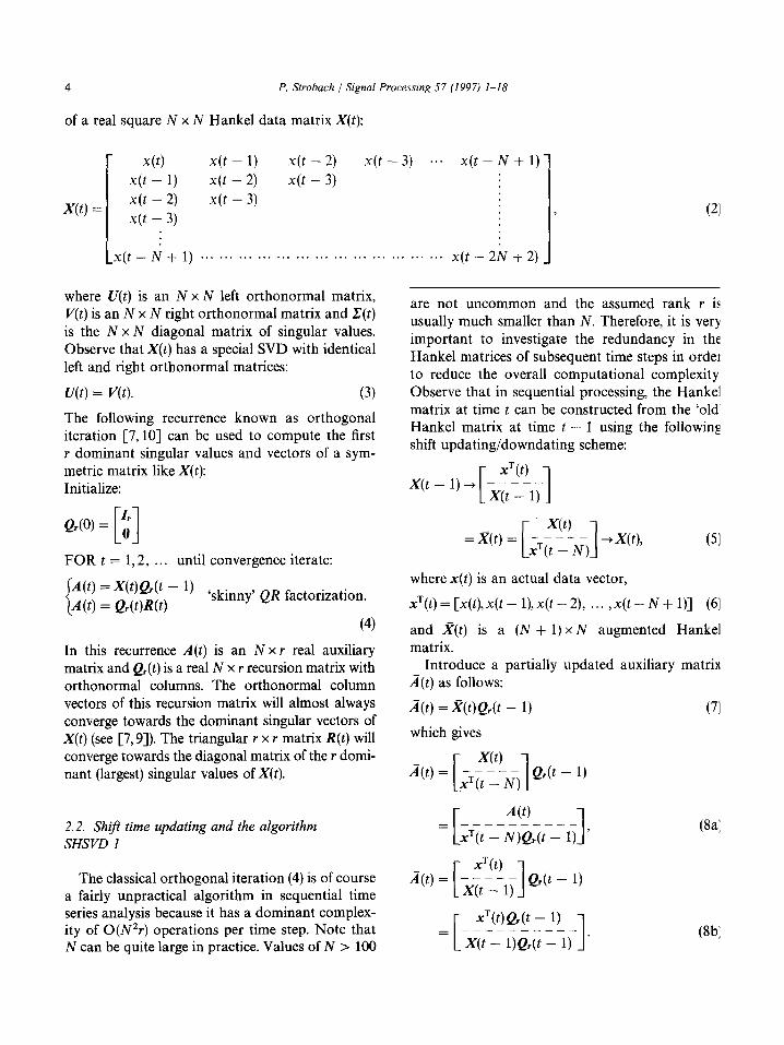
The following recurrence known as orthogonal iteration [7, lo] can be used to compute the first Y dominant singular values and vectors of a sym- metric matrix like X(t): Initialize:

FOR t = 1,2, . . . until convergence iterate:

= X(t)Q,@ - 1) = Q4W@)

‘skinny’ QR factorization.

(4)

In this recurrence A(t) is an N x r real auxiliary matrix and Qr(t) is a real N x r recursion matrix with orthonormal columns. The orthonormal column vectors of this recursion matrix will almost always converge towards the dominant singular vectors of X(t) (see [7,9]). The triangular r x r matrix R(t) will converge towards the diagonal matrix of the r domi- nant (largest) singular values of X(t).

2.2. Shift time updating and the algorithm SHSVD 1

The classical orthogonal iteration (4) is of course a fairly unpractical algorithm in sequential time series analysis because it has a dominant complex- ity of O(N2r) operations per time step. Note that N can be quite large in practice. Values of N > 100

1

(21

are not uncommon and the assumed rank r is usually much smaller than N. Therefore, it is very important to investigate the redundancy in the Hankel matrices of subsequent time steps in order to reduce the overall computational complexity Observe that in sequential processing, the Hankel matrix at time t can be constructed from the ‘old Hankel matrix at time t - 1 using the following shift updating/downdating scheme:

where x(t) is an actual data vector,

xT(t)=[x(t),x(t-1),x(&2), . . ..x(t-N+l)] (6)

and X(t) is a (N + 1) x N augmented Hankel matrix.

Introduce a partially updated auxiliary matrix A(t) as follows:

A(t) = X(t)Q& - 1)

which gives

(71

40

= xT(t - N)Q,(t - 1) [---------- 1 ’ T

A(t) = i;!ily Q& - 1) [ 1

xT(t)Qr(t - 1)

= X(t - l)Q,(t - 1) C---------- 1 . W:

P. Strobach / Signal Processing 57 (1997) 1-18 5

The goal is to express A(t) directly in terms of the ‘old’ auxiliary matrix A(t - 1) plus some update depending on the data vector x(t).

For this purpose, introduce the following rank r approximant of X(t):

X(r) = Q,(t)R(t)Q:(t - 1). (9)

This approximant satisfies the following consist- ency relation:

A(t) = X(t)Qr(t - 1) = X(t)Q,(t - 1). (10)

Surprisingly enough, we can replace X(t) by X(r) without changing A(t). Indeed, X(t) as defined in (9) is an optimal rank r approximant in the sense of sequential orthogonal iteration. See the detailed discussion in [13]. Replace X(t - 1) in (8b) by X(t - 1) and define

A(r)

[----------

x’(t)Qr(t - 1)

i’(t - N)Q,.(t - 1) l=[---------- X(t - l)Q,(t - 1) 1 ’ (11) where iT(t - N) = [0 . . . 0, l]X(t - 1) is just the bottom row vector of X(t - 1). Clearly,

X(t - l)Q$ - 1)

= Qr(t - l)R(t - l)Q:(t - 2)Q,(t - 1)

= A(t - l)@(t - l),

where

(12)

o(t) = Q:(t - l)Qr(t) (13)

is just an r x r matrix of cosines. This matrix plays a key role in fast sequential orthogonal iteration because it determines the distance between two subsequent subspaces. Further define

h(t) = QT(t - 1)x(t). (14)

Realize that QT(t - 1) acts like a data compressor on the input data vector x(t). All the subspace or signal relevant information in x(t) is concentrated in a vector h(t) of much smaller dimension r. This initial data compaction step is characteristic for almost all fast subspace tracking algorithms [ 12,131. Likewise, we define

a(t) = Q:(t - l)f(t - N). (IS)

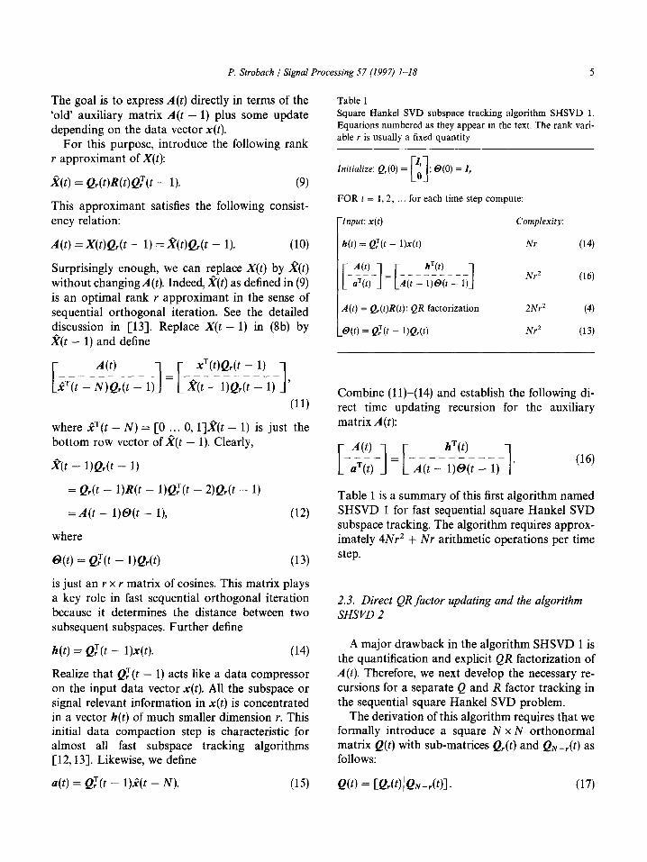
Table 1 Square Hankel SVD subspace tracking algorithm SHSVD 1. Equations numbered as they appear in the text. The rank vari- able r is usually a fixed quantity

4 Initialize: Q,(O) = o ; Q(0) = Z, [I FOR t = 1,2, for each time step compute:

7nput: x(t) Complexity:

h(t) = @(t - 1)x(t) Nr (14)

A(t) = Q,(t)R(t): QR factorization

.@(t) = QfO - l,Q&)

2Nr=

Nr*

Combine (1 l)-(14) and establish the following di- rect time updating recursion for the auxiliary matrix A(t):

Table 1 is a summary of this first algorithm named SHSVD 1 for fast sequential square Hankel SVD subspace tracking. The algorithm requires approx- imately 4Nr2 + Nr arithmetic operations per time step.

2.3. Direct QR factor updating and the algorithm SHSVD 2

A major drawback in the algorithm SHSVD 1 is the quantification and explicit QR factorization of A(t). Therefore, we next develop the necessary re- cursions for a separate Q and R factor tracking in the sequential square Hankel SVD problem.

The derivation of this algorithm requires that we formally introduce a square N x N orthonormal matrix Q(t) with sub-matrices Q,(t) and QN_Jt) as follows:

6 P. Strobach 1 Signal Processing 57 (1997) l-18

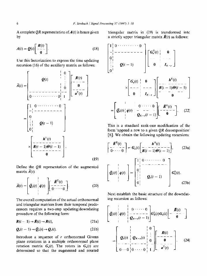
A complete QR representation ofA (t) is hence given

by

A(t) = Q(t) :i! [ 1 (18)

Use this factorization to express the time updating recursion (16) of the auxiliary matrix as follows:

A(t) = I O

hT (0

x Iz(t - 1)@(t - 1) [1 . ---------

0

R(t)

0

aT@)

(19)

Define the QR representation of the augmented matrix A(t):

A(t) = &(t) I 4(t)

[ ; I RT(t) [ 1 ;- - -0 .

, . . . (20)

The overall computation of the actual orthonormal and triangular matrices from their temporal prede- cessors requires a two-step updatingldowndating procedure of the following form:

R(t - 1) -+ R(t) --f R(t),

QrO - 1) -+ &Cd + Q&l.

Introduce a sequence of r orthonormal Givens plane rotations in a multiple orthonormal plane rotation matrix G,,(t). The rotors in G,(t) are determined so that the augmented and rotated

triangular matrix in (19) is transformed inta a strictly upper triangular matrix R(t) as follows:

-1/o . . . . . . . . . . 0

_/ ______~__

o/ ; / Q(t - 1)

-O/

hT(t)

II--------- R(t - l)Q(t - 1) ---_--__-

0 L

I ().....(-J

/ - ~ -- __

1

ITT(t)

/ Q&t - 1) --. -- . (22)

This is a standard rank-one modification of the form ‘append a row to a given QR decomposition’ [6]. We obtain the following updating recursions:

(23a)

i

QSd I

1 1 o--y_“_ 0;

4(t) = : I G:(t). f I Qr(t - 1)

_O! (23b)

Next establish the basic structure of the downdat- ing recursion as follows:

Ez

10

-!----- II R(t) QJt) 1 QN_Jt) / ’

10 - - 0 - -

o olo . o 1-1 ----- . . 1 . . . I UT(t) 1 . (24)

P. Strobach / Signal Processing 57 (1997) 1-18 I

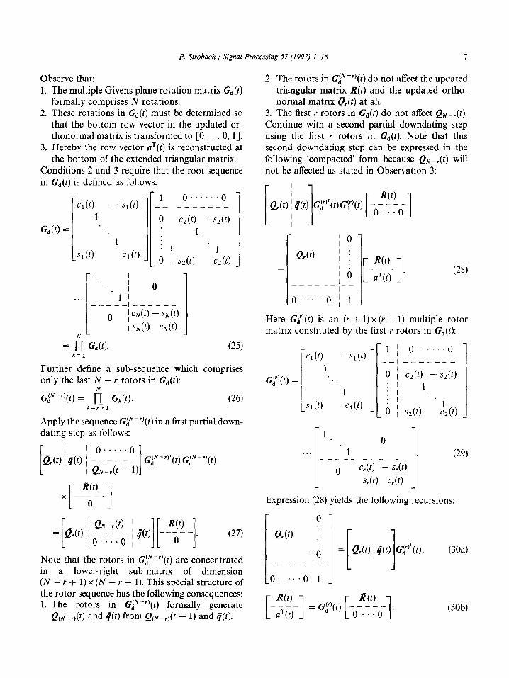
Observe that: 1. The multiple Givens plane rotation matrix Gd(t)

formally comprises N rotations. 2. These rotations in Gd(t) must be determined so

that the bottom row vector in the updated or- thonormal matrix is transformed to [0 . . . 0, 11.

3. Hereby the row vector aT(t) is reconstructed at the bottom of the extended triangular matrix.

Conditions 2 and 3 require that the root sequence in Gd(t) is defined as follows:

1 0 ; CN(Q - SN@) I slv(t) clv(t)

= kfil G(t).

Further define a sub-sequence whit only the last N - r rotors in GJt):

Gf-I)(t) = i”l Gk(t). k=r+l

(25)

ch comprises

(26)

Apply the sequence CAN-“(t) in a first partial down- dating step as follows:

g(t) I _‘_’ : 1 I! / Qiv-r(t - 1)

GiN-“‘(t) @‘-r)(t)

m X [-----I 0

= (27)

Note that the rotors in CAN-*‘(t) are concentrated . a lower-right sub-matrix of dimension k - r + 1) x (N - r + 1). This special structure of the rotor sequence has the following consequences: 1. The rotors in GiN-*)(t) formally generate

QcN-&) and I(t) from QcN-& - 1) and (7(t).

2. The rotors in CT-‘) (t) do not affect the updated triangular matrix R(t) and the updated ortho- normal matrix Qr(t) at all.

3. The first r rotors in Cd(t) do not affect QN_,(t).

Continue with a second partial downdating step using the first I rotors in Gd(t). Note that this second downdating step can be expressed in the following ‘compacted’ form because QN_,(t) will not be affected as stated in Observation 3:

1 O QAt) ; i =1------\--l R(t) I : ---- '0 [ 1 d(t) .

(28) Lo .....o ; 1 J

Here G!‘(t) is an (I + 1) x (r + 1) multiple rotor matrix constituted by the first r rotors in Gd(t):

G!‘(t) =

Cl w - s,(t) 1

1

Q(t) ... ,: cl(t)

I-

l / O......O __, _-_-___ 0 / m - m : I : 1

1

: ’

0 ) sz(t) c’, 0)

1 1 I . . j 0 I . . .

i

__L ---_-- . (29)

0 ;c,(t) - 4)

’ s,(t) c,(t) 1 Expression (28) yields the following recursions:

/ O Qr(t)

C$“‘(t), (304 -O. .. 9 l -

R(t) L---- 4t) = G”‘(t)

R(t) _ _ _ _ _

d i 1 0 0’ . . . WW

8 P. Strobach J Signal Processing 57 (1997) 1-18

At this point it is very important to realize that we could compute the second partial downdating re- cursion (30a), (30b) without performing the first partial downdating step (27) explicitly if only q(t) would be known and available because the explicit computation of @_ r,(t) is not necessarily required in the overall recursion. In fact, it can be shown that q(t) can be computed without determining the N - Y rotors in Gy-*’ (t) explicitly. This property of the downdating recursions is the key to a fast direct QR factor based sliding window Hankel SVD sub- space tracker.

To see this, investigate the structure of the partial downdating rotor Gji’)(t). We may verify that

where

ok = fi Cj(t), 1 < k < r, (324 j=l

bT(t) = CPl(O, Bz(t), ... ,MOl,

flj(r) = sj(t)Yj- l(t), l <j d y. (32b)

The detailed expressions for @d(t) and z(t) are unin- teresting in this context.

Substitute (31) into (30a) to obtain

= Q(t)@,@) + %(t)4(t)zT(t) ; Q&)!+) + ?b@)@) . I I

(33)

From (33) we deduce

!&co [-----I o...o = &r@)@d@) + ?r(t)4(t)zT@), (344

W)

Next substitute (31) into (30b):

Q;f (0 / Yr(OZ@)

/P(t) i J+(t) 1 m ----- ________~ [ 1 O . . . O

@(t)R(t) = [-----I BT(t)R(t) .

(35)

This yields

R(t) = @(t@(t),

G(t) = /P(t)R(t).

The following observations can be made:

(364

(W

Expression (34a) is a typical rank-l modification of a type which occurs frequently in fast sub- space tracking (see the detailed discussion in [13]). In fact, @d(t) can be interpreted as a ‘par- tial downdating rotor’. More important is expression (36b). Note that the elements of a(t) can be computed via (15) or, using (19) via

UT(t) = [O . . . 0, l]Ql(t - l)R(t - l)Q(t - 1).

(37)

Since the elements of u(t) are hence available before the downdating rotors produce them, we can employ (36b) to compute /?(t) using simple back substitution (recall that l?(t) is known and triangular). Once j?(t) is known, we can determine the r ro- tors in G!‘(t) together with the desired y*(t) using (32a) and (32b) as follows:

s1(t) = Pt(r), cl(r) = (1 - s:(0P2, 71(t) =c1(0

FORj = 2,3, . . . ,r

sj(t) = Bj(t)/Yj- l(t), Cj(t) =U - sf(t))"2t

Yj(t)=cj(t)?j(t - l). (38)

P. Strobach / Signal Processing 57 (1997) I-18 9

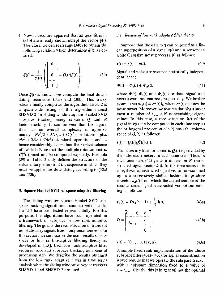
4. Now it becomes apparent that all quantities in (34b) are already known except the vector q(t). Therefore, we can rearrange (34b) to obtain the following relation which determines 4(t), as de- sired:

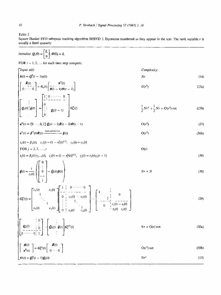
Once 4(t) is known, we compute the final down- dating recursions (30a) and (30b). This tricky scheme finally completes the algorithm. Table 2 is a quasi-code listing of this algorithm named SHSVD 2 for sliding window square Hankel SVD subspace tracking using separate Q and R factor tracking. It can be seen that the algori- thm has an overall complexity of approxi- mately Nr2/2 + 3Nr/2 + 0(r3) rotations plus Nr2 + 2Nr + O(r3) standard operations and is hence considerably faster than the explicit scheme of Table 1. Note that the multiple rotation matrix G!‘(t) must not be computed explicitly. Formula (29) in Table 2 only defines the structure of the r elementary rotors and the sequence in which they must be applied for downdating according to (30a) and (30b).

3. Square Hankel SVD subspace adaptive filtering

The sliding window square Hankel SVD sub- space tracking algorithms as summarized in Tables 1 and 2 have been tested experimentally. For this purpose, the algorithms have been operated in a framework of subspace or low rank adaptive filtering. The goal is the reconstruction of transient nonstationary signals from noisy measurements. In this section, we summarize the main results of sub- space or low rank adaptive filtering theory as developed in [13]. Each low rank adaptive filter requires rank and subspace tracking as a central processing step. We describe the results obtained from the low rank adaptive filters in time series analysis when the sliding window subspace trackers SHSVD 1 and SHSVD 2 are used.

3. I. Review of low rank adaptive jilter theory

Suppose that the data x(t) can be posed as a lin- ear superposition of a signal s(t) and a zero-mean white Gaussian noise process n(t) as follows:

x(t) = s(t) -t n(t). (40)

Signal and noise are assumed statistically indepen- dent, hence

Q(r) = Q,(r) + @p,(r), (41)

where G(t), a,(t) and cP,(t) are data, signal and noise covariance matrices, respectively. We further assume that ai, = 02(t)ZN where a2(t) denotes the noise power. Moreover, we assume that a,(t) has at most a number of r,,x < N nonvanishing eigen- values. In this case, a reconstruction s*(t) of the signal in x(t) can be computed in each time step as the orthogonal projection of x(t) onto the column space of Q*(t) as follows:

s*(t) = Q&,Q~W@,. (42)

The necessary transform matrix Qr(t) is provided by the subspace trackers in each time step. Thus, in each time step, (42) yields a dimension N recon- structed signal vector s*(t). In the time series data case, these reconstructed signal vectors are summed up in a successively shifted fashion to produce a vector sA(t) from which the actual sample of the reconstructed signal is extracted via bottom pinn- ing as follows:

s‘4(t) = Ds‘4(t - 1) + ; i(t), 0.. d 0 ,_ - - D=

I--- 1 10 > IN-1 I .

I . I 0

(43a)

(4W

g(t) = [O . . . 0, l]s,4(t). (43c)

A simple fixed rank implementation of the above subspace filter (43a)-(43c) for signal reconstruction would require that we operate the subspace tracker with a subspace dimension fixed to a value of Y = rmax. Clearly, this is in general not the optimal

10

Table 2

P. Strobach J Signal Processing 57 (1997) I-18

Square Hankel SVD subspace tracking algorithm SHSVD 2. Equations numbered as they appear in the text. The rank variable Y is usually a fixed quantity

Initiaiize: Q”(O) = [I ; ;@(O) =z, FOR t = 1,2, . . . for each time step compute:

2(t) = [O IO, 11 Q*(t - l)R(t - l)@(t - 1)

aT(t) z.z ~T(~)~(~)~ j(t)

Sl(Q = Bl(d, c,(t) = (1 - s:w2, r,(t) = c,(t)

FORj=2,3, . . ..Y

Sj(t) = ~j(t)/$fj- t(t), Cj(t) = (1 - s~jt))“‘, ';j(t) = Cj(t)yj(t - 1)

‘c*(t) -St(f) 1 / ().‘....()

_._/ _--__-.- 1

0 j cd4 - sz(t) I~:1 f. I[.~ I / 0

'. .~,

1 1, _____I__--__

: I

cl(t) :I '1 0 j c,(r) - s,(t)

0 ) s&l C2(4 ' s&) c,(t)

Complexity:

Nr

W)

(14)

(238)

i Nr2 + 5 Nr f O(rZ) rot (23b)

W2) (37)

wt (36b)

O(r)

Nr-tN

(38)

(38)

(29)

Nr + O(r) rot (30a)

.@(t) = Q% - l,Qr@,

O(r2) rot

Nr2

(30b)

(13)

P. Sfrobach { Signal Processing 57 (1997) I-18 11

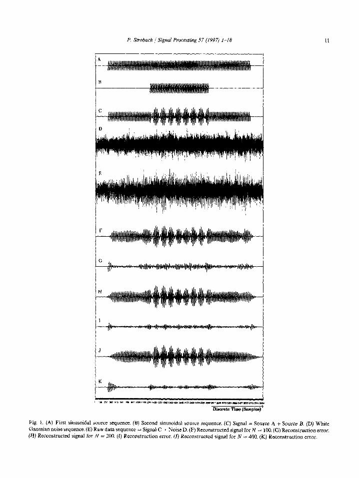
Fig. 1. (A) First sinusoidal source sequence. (B) Second sinusoidal source sequence. (C) Signal = Source A + Source B. (0) White Gaussian noise sequence. (E) Raw data sequence = Signal C + Noise D. (F) Reconstructed signal for N = 100. (G) Reconstruction error. (H) Reconstructed signal for N = 200. (I) Reconstruction error. (J) Reconstructed signal for N = 4cM. (K) Reconstruction error.

P. Strobach / Signal Processing 57 (1997) I-18

Adaptive Threshold

1 131 261 3w 521 61 781 911 1W1117113M14711561188118211951aOBlp11p4124712801~l~l~312132513381351138413TT13801 \

Discrete Time (Samples) ’

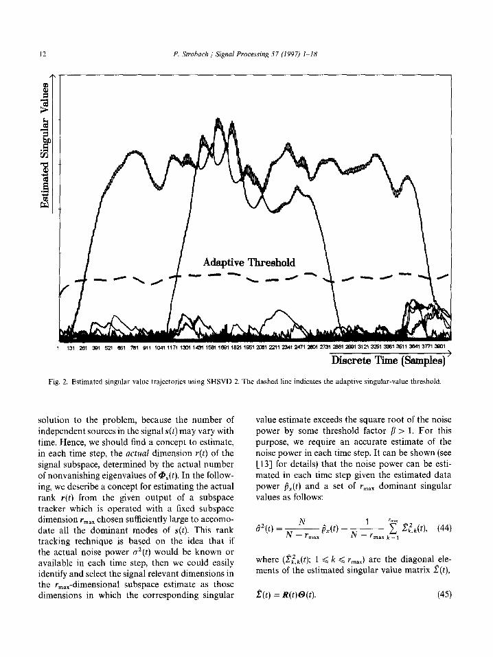
Fig. 2. Estimated singular value trajectories using SHSVD 2. The dashed line indicates the adaptive singular-value threshold.

solution to the problem, because the number of independent sources in the signal s(t) may vary with time. Hence, we should find a concept to estimate, in each time step, the actual dimension r(t) of the signal subspace, determined by the actual number of nonvanishing eigenvalues of es(t). In the follow- ing, we describe a concept for estimating the actual rank r(t) from the given output of a subspace tracker which is operated with a fixed subspace dimension rmax chosen sufficiently large to accomo- date all the dominant modes of s(t). This rank tracking technique is based on the idea that if the actual noise power c?(t) would be known or available in each time step, then we could easily identify and select the signal relevant dimensions in the Y,,,- dimensional subspace estimate as those dimensions in which the corresponding singular

value estimate exceeds the square root of the noise power by some threshold factor p > 1. For this purpose, we require an accurate estimate of the noise power in each time step. It can be shown (see [13] for details) that the noise power can be esti- mated in each time step given the estimated data power &(t) and a set of r,,, dominant singular values as follows:

where (C&(t); 1 < k f rmax) are the diagonal ele- ments of the estimated singular value matrix f(t),

f(t) = R(t)@(t). (45)

P. Strobach / Signal Processing 57 (1997) l-18 13

1 126 251 378 501 628 751 876103111281zj1~3761501182817511578an1t128zL51plB25MzBzB27512876rxn3128325133783501382837513878

Discrete Time (Samples) ’

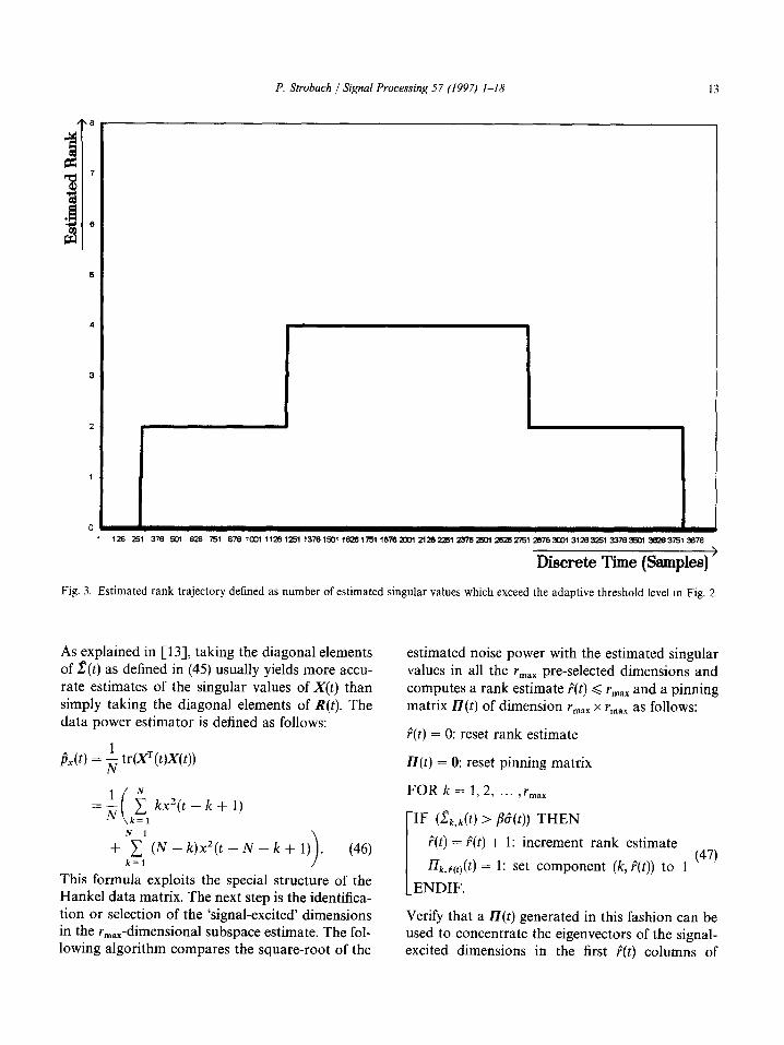
Fig. 3. Estimated rank trajectory defined as number of estimated singular values which exceed the adaptive threshold level in Fig. 2.

As explained in [13], taking the diagonal elements of f(t) as defined in (45) usually yields more accu- rate estimates of the singular values of X(t) than simply taking the diagonal elements of R(t). The data power estimator is defined as follows:

&(t) = $ tr(XT(t)X(t))

= ;( ; kx’(t - k + 1) “ \k=l

N-l

+ ,zl (N - k)x’(t - N - k + 1) >

. (46)

This formula exploits the special structure of the Hankel data matrix. The next step is the identifica- tion or selection of the ‘signal-excited’ dimensions in the rmalr -dimensional subspace estimate. The fol- lowing algorithm compares the square-root of the

estimated noise power with the estimated singular values in all the rmax pre-selected dimensions and computes a rank estimate +(t) < rmax and a pinning matrix n(t) of dimension rmax x rmax as follows:

v^(t) = 0: reset rank estimate

ZZ(t) = 0: reset pinning matrix

FOR k = 1,2, . . . ,I,,_~

I

IF @,,,(t) > pi?(t)) THEN

t(t) = P(t) + 1: increment rank estimate

17k,p(tj(t) = 1: Set component (k, r+(t)) to 1 (47)

ENDIF.

Verify that a n(t) generated in this fashion can be used to concentrate the eigenvectors of the signal- excited dimensions in the first F(t) columns of

! !1 ~‘,“lr ” i! Ii!’ t ‘I’ ,i 14,

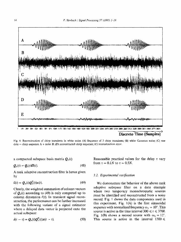
Fig. 4. ~econstructi#n of chirp transients in white noise. (A) Sequence of 3 chirp transients; (B) white Gaussian noise; (C) raw data = chirp sequence A -!- noise B; (D) reconstructed chirp sequence; f-E) reconstruction error.

a compacted subspace basis matrix Q%(t):

Q&> = Q&)~(G (48)

A rank adaptive reconstruction filter is hence given

by

$6) = Q=(~)Q~~~)~(~). (49)

Ctearly, the weighted summation ofc~l~mn vectors of Q*(t) according to (49) is only computed up to column dimension r*(t). In transient signal recon- struction, the ~erform~ce can be further increased with the following variant of a signal estimator where a delayed data vector is projected onto the actual subspace:

@ - z) = Q~(~)Q~(~)~(~ - ‘t). (50)

Reasonable practical values for the delay z vary from z = 0.1N to z = 0.5N.

We demonstrate the behavior of the above rank adaptive subspace filter on a data example where two temporary monochromatic sources must be identified and reconstructed from a noisy record. Fig. 1 shows the data components used in this experiment. Fig. l(A) is the first sinusoidal sequence with normalized frequency o1 = lo”. This source is active in the time interval 300 < t d 3700. Fig. l(B) shows a second source with w2 = 12”. This source is active in the interval 1300 G

P. Strobach / Signal Processing 57 (1997) I-18 15

1 131 2El 381 521 651 781 811 10411171lmls31lserlwlls~lssraoelmlpol24712BM~laBB128813121325133813511384137713801

Discrete Time (Samples) >

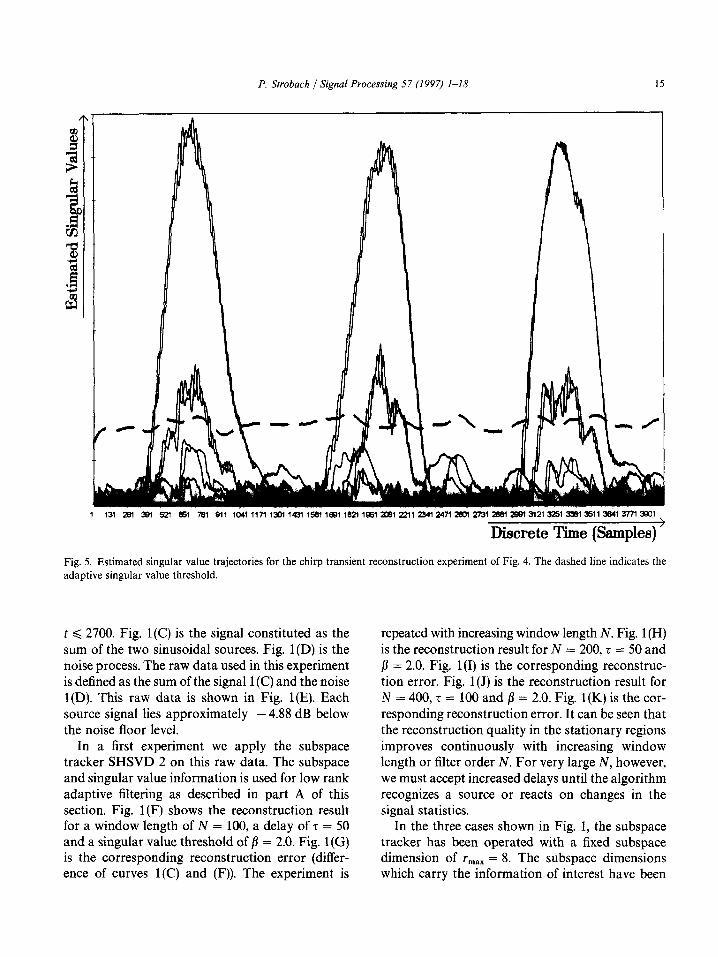
Fig. 5. Estimated singular value trajectories for the chirp transient reconstruction experiment of Fig. 4. The dashed line indicates the adaptive singular value threshold.

t < 2700. Fig. l(C) is the signal constituted as the sum of the two sinusoidal sources. Fig. l(D) is the noise process. The raw data used in this experiment is defined as the sum of the signal 1 (C) and the noise l(D). This raw data is shown in Fig. l(E). Each source signal lies approximately - 4.88 dB below the noise floor level.

In a first experiment we apply the subspace tracker SHSVD 2 on this raw data. The subspace and singular value information is used for low rank adaptive filtering as described in part A of this section. Fig. l(F) shows the reconstruction result for a window length of N = 100, a delay of z = 50 and a singular value threshold of j? = 2.0. Fig. 1 (G) is the corresponding reconstruction error (differ- ence of curves l(C) and (F)). The experiment is

repeated with increasing window length N. Fig. 1 (H) is the reconstruction result for N = 200, r = 50 and fi = 2.0. Fig. l(1) is the corresponding reconstruc- tion error. Fig. l(J) is the reconstruction result for N = 400, r = 100 and fl = 2.0. Fig. l(K) is the cor- responding reconstruction error. It can be seen that the reconstruction quality in the stationary regions improves continuously with increasing window length or filter order N. For very large N, however, we must accept increased delays until the algorithm recognizes a source or reacts on changes in the signal statistics.

In the three cases shown in Fig. 1, the subspace tracker has been operated with a fixed subspace dimension of I,,, = 8. The subspace dimensions which carry the information of interest have been

16 P. Strobach / Signal Processing 57 (1997) l-18

1 126 251 376 501 6-a 751 876 10011126125113761501162617511876zun 21282251237825012EB2751287830013128325133763sOl382837513376

Discrete Time (Samples

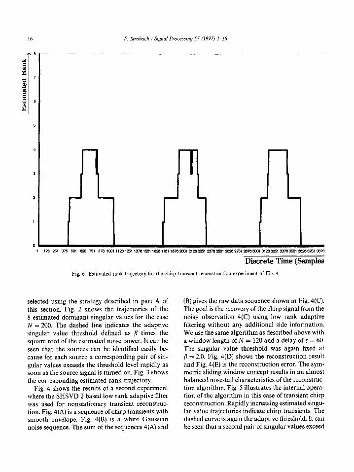
Fig. 6. Estimated rank trajectory for the chirp transient reconstruction experiment of Fig. 4.

selected using the strategy described in part A of this section. Fig. 2 shows the trajectories of the 8 estimated dominant singular values for the case N = 200. The dashed line indicates the adaptive singular value threshold defined as p times the square root of the estimated noise power. It can be seen that the sources can be identified easily be- cause for each source a corresponding pair of sin- gular values exceeds the threshold level rapidly as soon as the source signal is turned on. Fig. 3 shows the corresponding estimated rank trajectory.

Fig. 4 shows the results of a second experiment where the SHSVD 2 based low rank adaptive filter was used for nonstationary transient reconstruc- tion. Fig. 4(A) is a sequence of chirp transients with smooth envelope. Fig. 4(B) is a white Gaussian noise sequence. The sum of the sequences 4(A) and

(B) gives the raw data sequence shown in Fig. 4(C). The goal is the recovery of the chirp signal from the noisy observation 4(C) using low rank adaptive filtering without any additional side information. We use the same algorithm as described above with a window length of N = 120 and a delay of r = 60. The singular value threshold was again fixed at p = 2.0. Fig. 4(D) shows the reconstruction result and Fig. 4(E) is the reconstruction error. The sym- metric sliding window concept results in an almost balanced nose-tail characteristics of the reconstruc- tion algorithm. Fig. 5 illustrates the internal opera- tion of the algorithm in this case of transient chirp reconstruction. Rapidly increasing estimated singu- lar value trajectories indicate chirp transients. The dashed curve is again the adaptive threshold. It can be seen that a second pair of singular values exceed

P. Strobach f Signal Processing 37 (1997) l-18 17

1 131 281 331 521 13% 751 @II 1041117113011431156118911821 1Q5120812Zll234124112Wl27312SS12EB13121325133813517364137713&X

Discrete Time (Samplee) ’

Fig. 7. Reconstruction of chirp transients in first order AR noise. (A) Sequence of 3 chirp transients;(B) first-order AR noise (p = 0.9); (C) raw data = chirp sequence A + noise B, (D) reconstructed chirp sequence; (E) reconstruction error.

the threshold level slightly around the center of the chirp transients. This is the consequence of the heavily nonstationary character of the chirp sig- nals: The algorithm partly employs 4 basis func- tions for signal reconstruction. This is also con- firmed by the corresponding estimated rank traject- ory which is shown in Fig. 6.

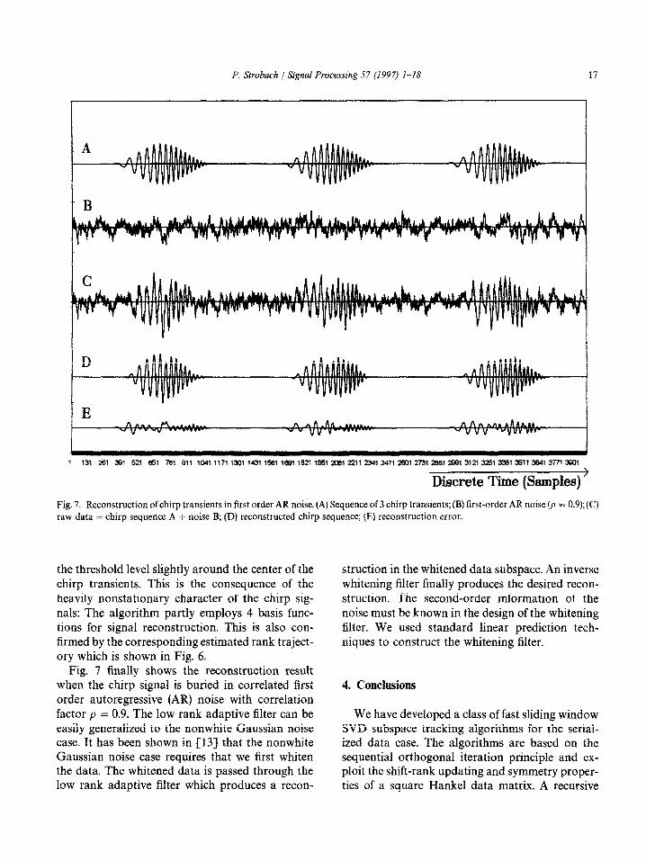
Fig. 7 finally shows the reconstruction result when the chirp signal is buried in correlated first order autoregressive (AR) noise with correlation factor p = 0.9. The low rank adaptive filter can be easily generalized to the nonwhite Gaussian noise case. It has been shown in [13] that the nonwhite Gaussian noise case requires that we first whiten the data. The whitened data is passed through the low rank adaptive filter which produces a recon-

struction in the whitened data subspace. An inverse whitening filter finally produces the desired recon- struction. The second-order information of the noise must be known in the design of the whitening filter. We used standard linear prediction tech- niques to construct the whitening filter.

4. Conclusions

We have developed a class of fast sliding window SVD subspace tracking algorithms for the serial- ized data case. The algorithms are based on the sequential orthogonal iteration principle and ex- ploit the shift-rank updating and symmetry proper- ties of a square Hankel data matrix. A recursive

18 P. Strobach / Signal Processing 57 (1997) l-18

sliding window SVD can be of great interest in many areas of signal analysis such as spectral es- timation, detection and adaptive filtering. The ap- plication of the algorithms has been demonstrated using two examples of low rank adaptive filtering for transient signal reconstruction from noisy ob- servations.

References

[l] F.L. Bauer, “Das Verfahren der Treppeniteration und verwandte Verfahren zur Losung algebra&her Eigen- wertprobleme”, Z. Angew. Math. Phys., Vol. 8, 1957, pp. 214235.

[Z] J.R. Bunch and C.P. Nielsen, “Updating the singular value decomposition”, Numer. Math., Vol. 31, 1978, pp. 111-129.

[3] M. Clint and A. Jennings, “A simultaneous iteration method for the unsymmetric eigenvalue problem”, J. Inst. Math. Appl., Vol. 8, 1971, pp. 111-121.

[4] P. Comon and G.H. Golub, “Tracking a few extreme singular values and vectors in signal processing”, Proc. IEEE, Vol. 78, No. 8, August 1990, pp. 1327-1343.

[S] E.M. Dowling, L.P. Ammann and R.D. DeGroat, “A TQR-iteration based adaptive SVD for real time angle and

frequency tracking”, IEEE Trans. Signal Process., Vol. 42, April 1994, pp. 914926.

[6] P.E. Gill, G.H. Golub, W. Murray and M.A. Saunders, “Methods for modifying matrix factorizations”, Math. Cornput., Vol. 28, No. 126, 1974, pp. 505-535.

[7] G.H. Golub and C.F. VanLoan, Matrix Computations, 2nd Edition, Johns Hopkins University Press, Baltimore, MD, 1989.

[S] I. Karasalo, “Estimating the covariance matrix by signal subspace averaging”, IEEE Trans. Acoust. Speech Signal Process., Vol. 34, February 1986, pp. 8-12.

[9] B.N. Parlett and W.G. Poole, “A geometric theory for the QR, LU and power iterations”, SIAM J. Numer. Anal., Vol. 10, No. 2, April 1973, pp. 389412.

[lo] G.W. Stewart, Introduction to Matrix Computations, Aca- demic Press, New York, 1974.

[ll] G.W. Stewart, “Methods of simultaneous iteration for calculating eigenvectors of matrices”, in: J.H. Miller, ed., Topics in Numerical Analysis II, Academic Press, New York, 1975, pp. 1699185.

[12] P. Strobach, “Bi-iteration SVD subspace tracking algo- rithms”, IEEE Trans. Signal Process., May 1997, To appear.

[13] P. Strobach, “Low rank adaptive filters”, IEEE Trans. Signal Process., Vol. 44, No. 12, December 1996, pp. 2932-2941.

[14] P. Strobach, “Fast recursive low rank linear prediction frequency estimation algorithms”, IEEE Trans. Signal Pro- cess., Vol. 44, No. 4, April 1996, pp. 834-847.