Embed Size (px)
Citation preview

SQL QUERY EVALUATIONCS121: Relational DatabasesFall 2017 – Lecture 12
Query Evaluation
¨ Last time:¤ Began looking at database implementation details¤ How data is stored and accessed by the database¤ Using indexes to dramatically speed up certain kinds of
lookups
¨ Today: What happens when we issue a query?¤ …and how can we make it faster?
¨ To optimize database queries, must understand what the database does to compute a result
2
Query Evaluation (2)
¨ Today:¤ Will look at higher-level query evaluation details¤ How relational algebra operations are implemented
n Common-case optimizations employed in implementations¤ More details on how the database uses these details to
plan and optimize your queries¨ There are always exceptions…
¤ e.g. MySQL’s join processor is very different from others¤ Every DBMS has documentation about query evaluation
and query optimization, for that specific database
3
SQL Query Processing
¨ Databases go through three basic steps:¤ Parse SQL into an internal representation of a plan¤ Transform this into an optimized execution plan¤ Evaluate the optimized execution plan
¨ Execution plans are generally based on the extended relational algebra¤ Includes generalized projection, grouping, etc.¤ Also some other features, like sorting results, nested
queries, LIMIT/OFFSET, etc.
4
Query Evaluation Example
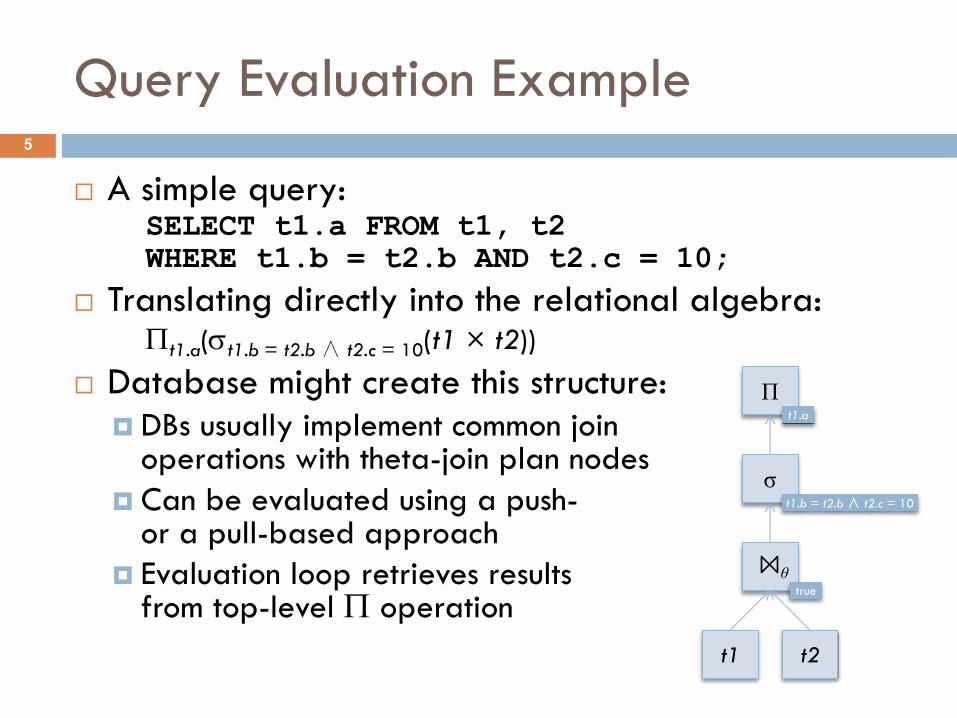
¨ A simple query:SELECT t1.a FROM t1, t2WHERE t1.b = t2.b AND t2.c = 10;
¨ Translating directly into the relational algebra:Pt1.a(st1.b = t2.b∧ t2.c = 10(t1 × t2))
¨ Database might create this structure:¤ DBs usually implement common join
operations with theta-join plan nodes¤ Can be evaluated using a push-
or a pull-based approach¤ Evaluation loop retrieves results
from top-level P operationt1 t2
θ
σt1.b = t2.b∧ t2.c = 10
Πt1.a
true
5
Query Optimization
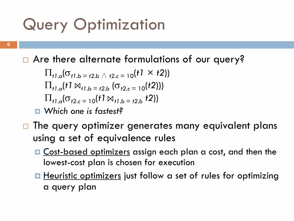
¨ Are there alternate formulations of our query?Pt1.a(st1.b = t2.b∧ t2.c = 10(t1 × t2))Pt1.a(t1 t1.b = t2.b (st2.c = 10(t2)))Pt1.a(st2.c = 10(t1 t1.b = t2.b t2))
¤ Which one is fastest?
¨ The query optimizer generates many equivalent plans using a set of equivalence rules¤ Cost-based optimizers assign each plan a cost, and then the
lowest-cost plan is chosen for execution¤ Heuristic optimizers just follow a set of rules for optimizing
a query plan
6
Query Evaluation Costs
¨ A variety of costs in query evaluation¨ Primary expense is reading data from disk
¤ Usually, data being processed won’t fit entirely into memory¤ Try to minimize disk seeks, reads and writes!
¨ CPU and memory requirements are secondary¤ Some ways of computing a result require more CPU and
memory resources than others¤ Becomes especially important in concurrent usage scenarios
¨ Can be other costs as well¤ In distributed database systems, network bandwidth must be
managed by query optimizer
7
Query Optimization (2)
¨ Several questions the optimizer has to consider:¤ How is a relation’s data stored on the disk?
n …and what access paths are available to the data?¤ What implementations of the relational algebra
operations are available to use?n Will one implementation of a particular operation be much
better or worse than another?¤ How does the database decide which query execution
plan is best?¨ Given the answers to these questions, what can we
do to make the database go faster?
8
Select Operation
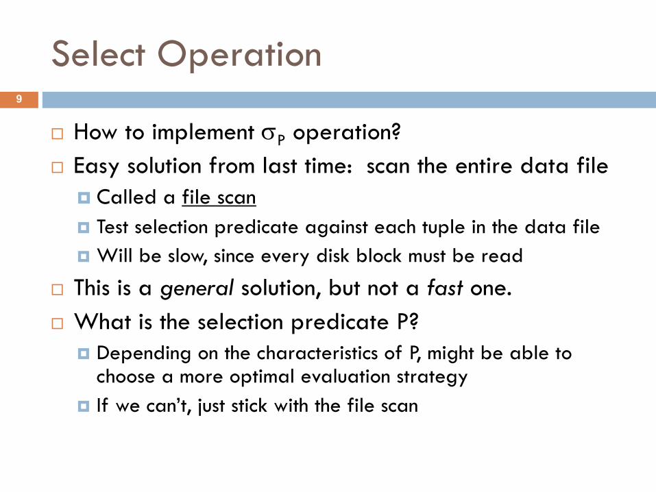
¨ How to implement sP operation?¨ Easy solution from last time: scan the entire data file
¤ Called a file scan¤ Test selection predicate against each tuple in the data file¤ Will be slow, since every disk block must be read
¨ This is a general solution, but not a fast one.¨ What is the selection predicate P?
¤ Depending on the characteristics of P, might be able to choose a more optimal evaluation strategy
¤ If we can’t, just stick with the file scan
9
Select Operation (2)
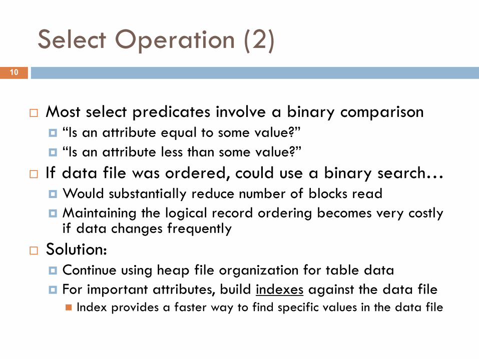
¨ Most select predicates involve a binary comparison¤ “Is an attribute equal to some value?”¤ “Is an attribute less than some value?”
¨ If data file was ordered, could use a binary search…¤ Would substantially reduce number of blocks read¤ Maintaining the logical record ordering becomes very costly
if data changes frequently¨ Solution:
¤ Continue using heap file organization for table data¤ For important attributes, build indexes against the data file
n Index provides a faster way to find specific values in the data file
10
Select Operation
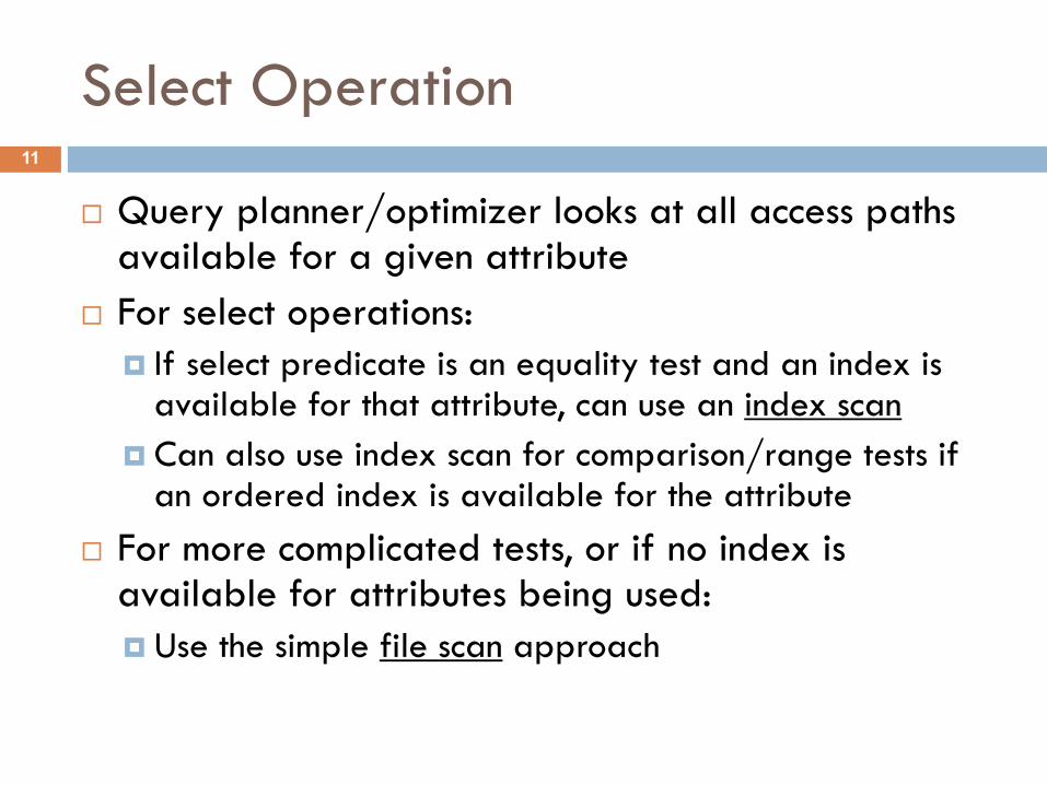
¨ Query planner/optimizer looks at all access paths available for a given attribute
¨ For select operations:¤ If select predicate is an equality test and an index is
available for that attribute, can use an index scan¤ Can also use index scan for comparison/range tests if
an ordered index is available for the attribute¨ For more complicated tests, or if no index is
available for attributes being used:¤ Use the simple file scan approach
11
Query Optimization Using Indexes
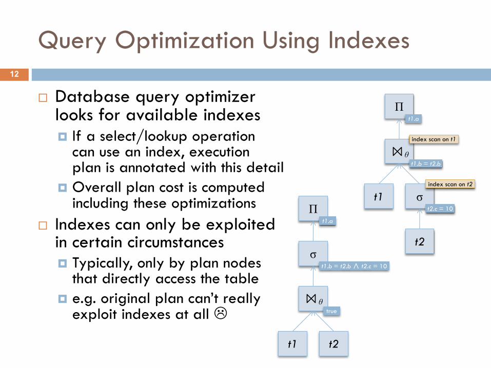
¨ Database query optimizerlooks for available indexes¤ If a select/lookup operation
can use an index, executionplan is annotated with this detail
¤ Overall plan cost is computedincluding these optimizations
¨ Indexes can only be exploitedin certain circumstances¤ Typically, only by plan nodes
that directly access the table¤ e.g. original plan can’t really
exploit indexes at all L
t1
t2
θ
σt2.c = 10
Πt1.a
t1.b = t2.b
index scan on t2
index scan on t1
t1 t2
θ
σt1.b = t2.b∧ t2.c = 10
Πt1.a
true
12
Project Operation
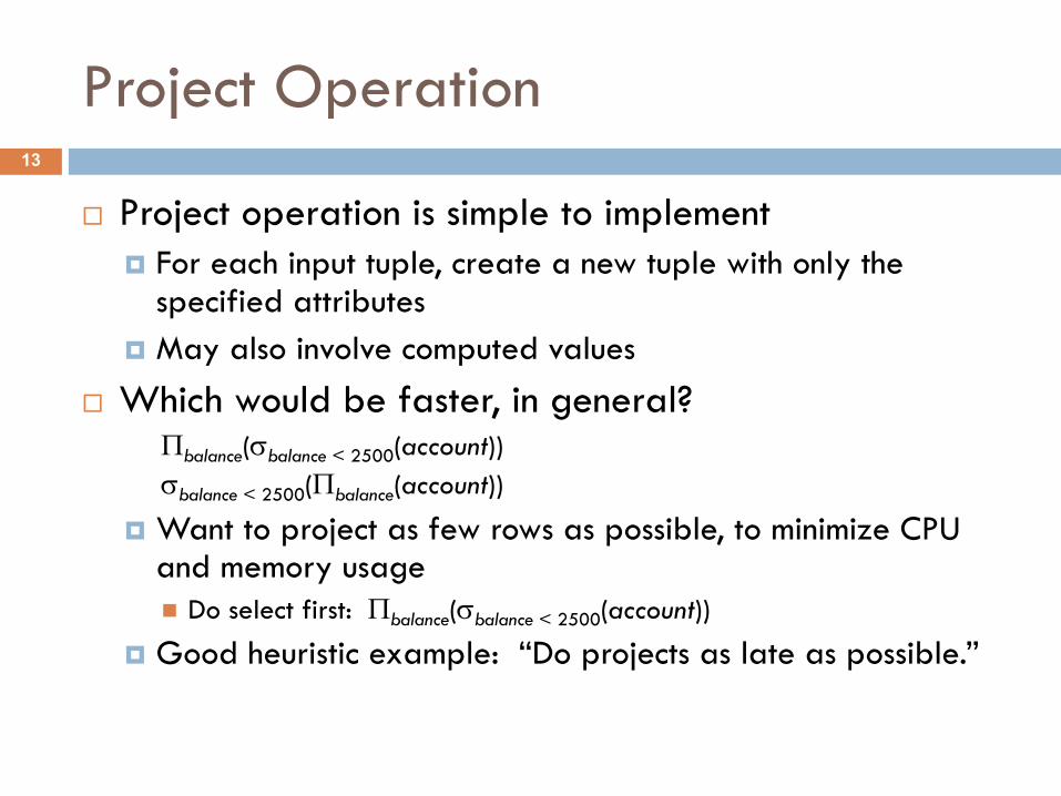
¨ Project operation is simple to implement¤ For each input tuple, create a new tuple with only the
specified attributes¤ May also involve computed values
¨ Which would be faster, in general?Pbalance(sbalance < 2500(account))sbalance < 2500(Pbalance(account))
¤ Want to project as few rows as possible, to minimize CPU and memory usagen Do select first: Pbalance(sbalance < 2500(account))
¤ Good heuristic example: “Do projects as late as possible.”
13
Sorting
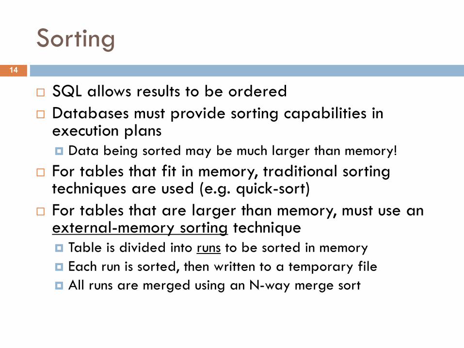
¨ SQL allows results to be ordered¨ Databases must provide sorting capabilities in
execution plans¤ Data being sorted may be much larger than memory!
¨ For tables that fit in memory, traditional sorting techniques are used (e.g. quick-sort)
¨ For tables that are larger than memory, must use an external-memory sorting technique¤ Table is divided into runs to be sorted in memory¤ Each run is sorted, then written to a temporary file¤ All runs are merged using an N-way merge sort
14
Sorting (2)
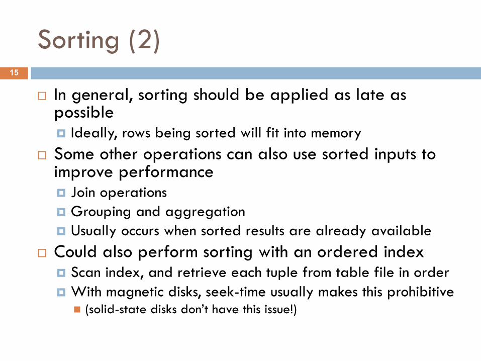
¨ In general, sorting should be applied as late as possible¤ Ideally, rows being sorted will fit into memory
¨ Some other operations can also use sorted inputs to improve performance¤ Join operations¤ Grouping and aggregation¤ Usually occurs when sorted results are already available
¨ Could also perform sorting with an ordered index¤ Scan index, and retrieve each tuple from table file in order¤ With magnetic disks, seek-time usually makes this prohibitive
n (solid-state disks don’t have this issue!)
15
Join Operations
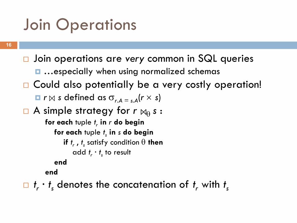
¨ Join operations are very common in SQL queries¤ …especially when using normalized schemas
¨ Could also potentially be a very costly operation!¤ r s defined as sr.A = s.A(r ´ s)
¨ A simple strategy for r q s :for each tuple tr in r do begin
for each tuple ts in s do beginif tr , ts satisfy condition q then
add tr · ts to resultend
end
¨ tr · ts denotes the concatenation of tr with ts
16
Nested-Loop Join
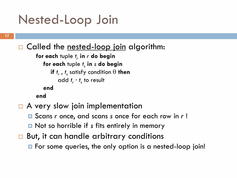
¨ Called the nested-loop join algorithm:for each tuple tr in r do begin
for each tuple ts in s do beginif tr , ts satisfy condition q then
add tr · ts to resultend
end
¨ A very slow join implementation¤ Scans r once, and scans s once for each row in r !¤ Not so horrible if s fits entirely in memory
¨ But, it can handle arbitrary conditions¤ For some queries, the only option is a nested-loop join!
17
Indexed Nested-Loop Join
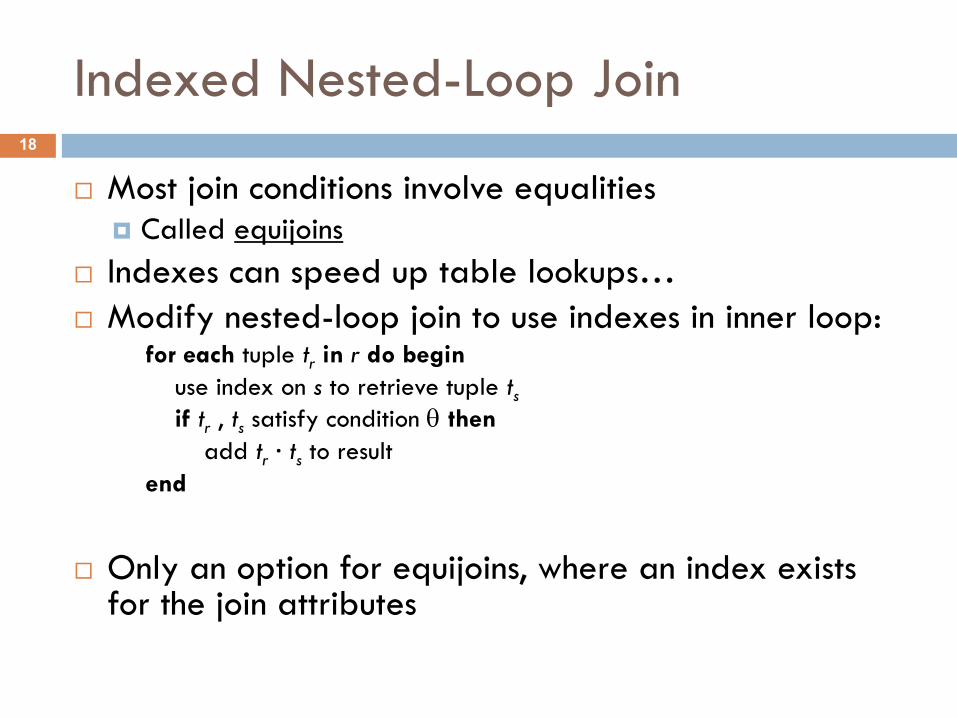
¨ Most join conditions involve equalities¤ Called equijoins
¨ Indexes can speed up table lookups…¨ Modify nested-loop join to use indexes in inner loop:
for each tuple tr in r do beginuse index on s to retrieve tuple tsif tr , ts satisfy condition q then
add tr · ts to resultend
¨ Only an option for equijoins, where an index exists for the join attributes
18
MySQL Join Processor
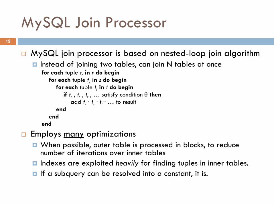
¨ MySQL join processor is based on nested-loop join algorithm¤ Instead of joining two tables, can join N tables at once
for each tuple tr in r do beginfor each tuple ts in s do begin
for each tuple tt in t do beginif tr , ts , tt , … satisfy condition q then
add tr · ts · tt · … to resultend
endend
¨ Employs many optimizations¤ When possible, outer table is processed in blocks, to reduce
number of iterations over inner tables¤ Indexes are exploited heavily for finding tuples in inner tables.¤ If a subquery can be resolved into a constant, it is.
19
MySQL Join Processor (2)
¨ Since MySQL join processor relies so heavily on indexes, what kinds of queries is it bad at?¤ Queries against tables without indexes… (duh)¤ Queries involving joins against derived relations (ugh!)¤ MySQL isn’t smart enough to save the derived relation into a
temporary table, then build an index against itn A common technique for optimizing complex queries in MySQL
¨ For more sophisticated queries, really would like more advanced join algorithms…¤ Most DBs include several other very powerful join algorithms¤ (Can’t add to MySQL easily, since it doesn’t use relational
algebra as a query-plan representation…)
20
Sort-Merge Join
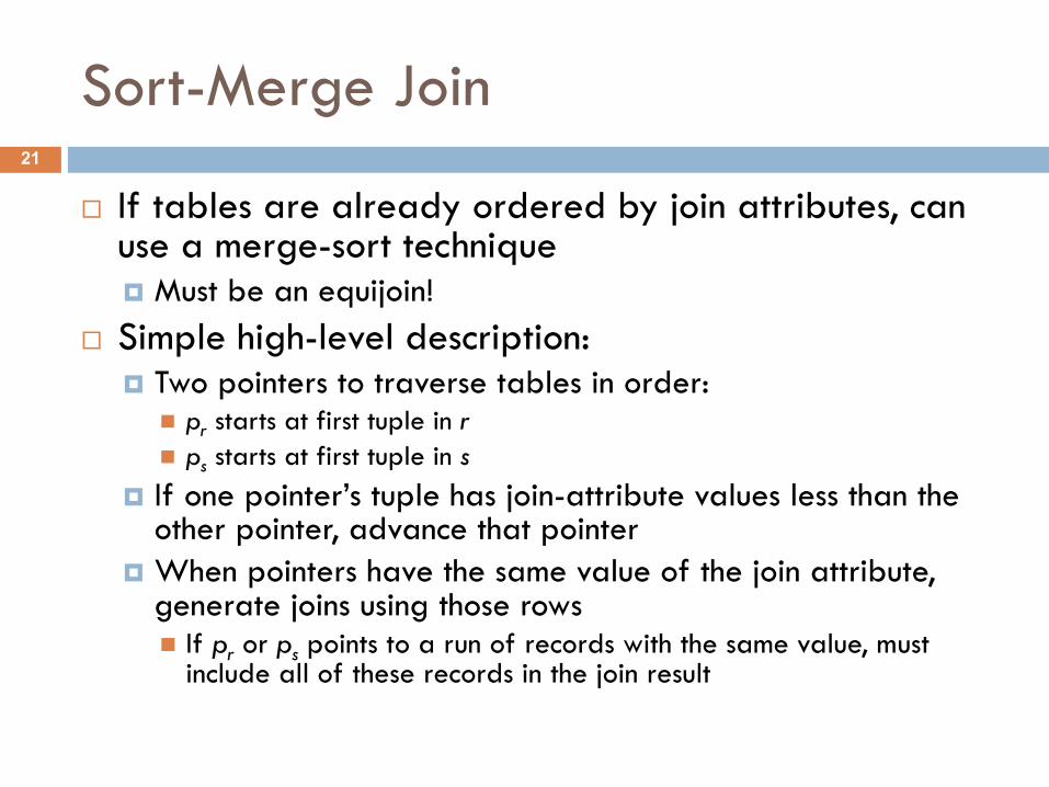
¨ If tables are already ordered by join attributes, can use a merge-sort technique¤ Must be an equijoin!
¨ Simple high-level description:¤ Two pointers to traverse tables in order:
n pr starts at first tuple in rn ps starts at first tuple in s
¤ If one pointer’s tuple has join-attribute values less than the other pointer, advance that pointer
¤ When pointers have the same value of the join attribute, generate joins using those rowsn If pr or ps points to a run of records with the same value, must
include all of these records in the join result
21
Sort-Merge Join (2)
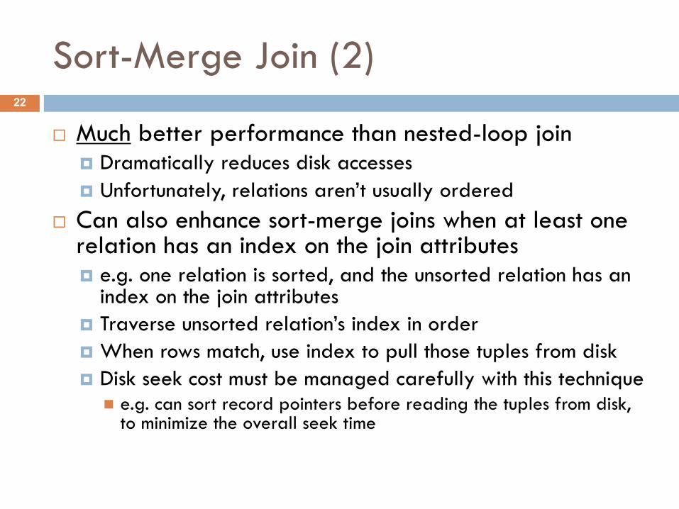
¨ Much better performance than nested-loop join¤ Dramatically reduces disk accesses¤ Unfortunately, relations aren’t usually ordered
¨ Can also enhance sort-merge joins when at least one relation has an index on the join attributes¤ e.g. one relation is sorted, and the unsorted relation has an
index on the join attributes¤ Traverse unsorted relation’s index in order¤ When rows match, use index to pull those tuples from disk¤ Disk seek cost must be managed carefully with this technique
n e.g. can sort record pointers before reading the tuples from disk, to minimize the overall seek time
22

Hash Join
¨ Another join technique for equijoins¨ For tables r and s :
¤ Use a hash function on the join attributes to divide rows of r and s into partitionsn Use same hash function on both r and s, of coursen Partitions are saved to disk as they are generatedn Aim for each partition to fit in memoryn r partitions: Hr1, Hr2, …, Hrn
n s partitions: Hs1, Hs2, …, Hsn
¤ Rows in Hri will only join with rows in Hsi
23
Hash Join (2)
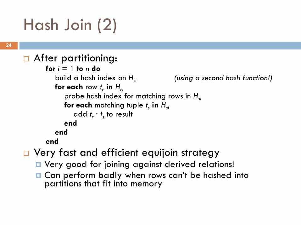
¨ After partitioning:for i = 1 to n do
build a hash index on Hsi (using a second hash function!)for each row tr in Hri
probe hash index for matching rows in Hsifor each matching tuple ts in Hsi
add tr · ts to resultend
endend
¨ Very fast and efficient equijoin strategy¤ Very good for joining against derived relations!¤ Can perform badly when rows can’t be hashed into
partitions that fit into memory
24
Outer Joins
¨ Join algorithms can be modified to generate left outer joins reasonably efficiently¤ Right outer join can be restated as left outer join¤ Will still impact overall query performance if many rows
are generated
¨ Full outer joins can be significantly harder to implement¤ Sort-merge join can compute full outer join easily¤ Nested loop and hash join are much harder to extend¤ Full outer joins can also impact query performance heavily
25
Other Operations
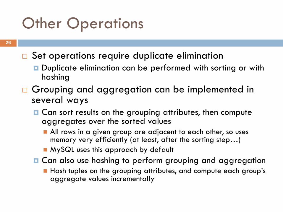
¨ Set operations require duplicate elimination¤ Duplicate elimination can be performed with sorting or with
hashing¨ Grouping and aggregation can be implemented in
several ways¤ Can sort results on the grouping attributes, then compute
aggregates over the sorted valuesn All rows in a given group are adjacent to each other, so uses
memory very efficiently (at least, after the sorting step…)n MySQL uses this approach by default
¤ Can also use hashing to perform grouping and aggregationn Hash tuples on the grouping attributes, and compute each group’s
aggregate values incrementally
26
Optimizing Query Performance
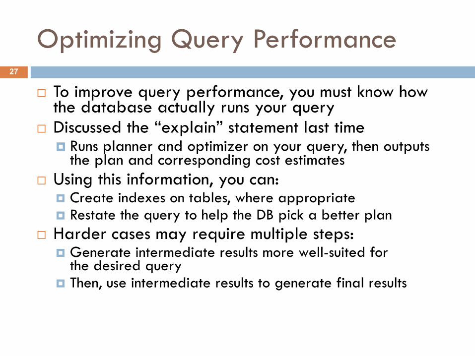
¨ To improve query performance, you must know how the database actually runs your query
¨ Discussed the “explain” statement last time¤ Runs planner and optimizer on your query, then outputs
the plan and corresponding cost estimates¨ Using this information, you can:
¤ Create indexes on tables, where appropriate¤ Restate the query to help the DB pick a better plan
¨ Harder cases may require multiple steps:¤ Generate intermediate results more well-suited for
the desired query¤ Then, use intermediate results to generate final results
27
Query Execution Example
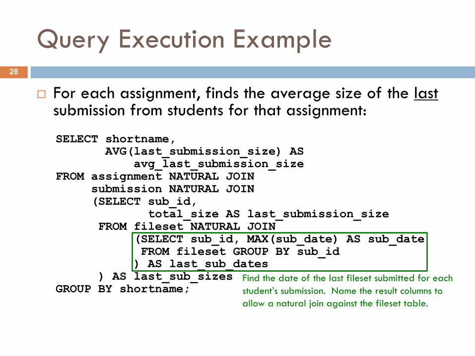
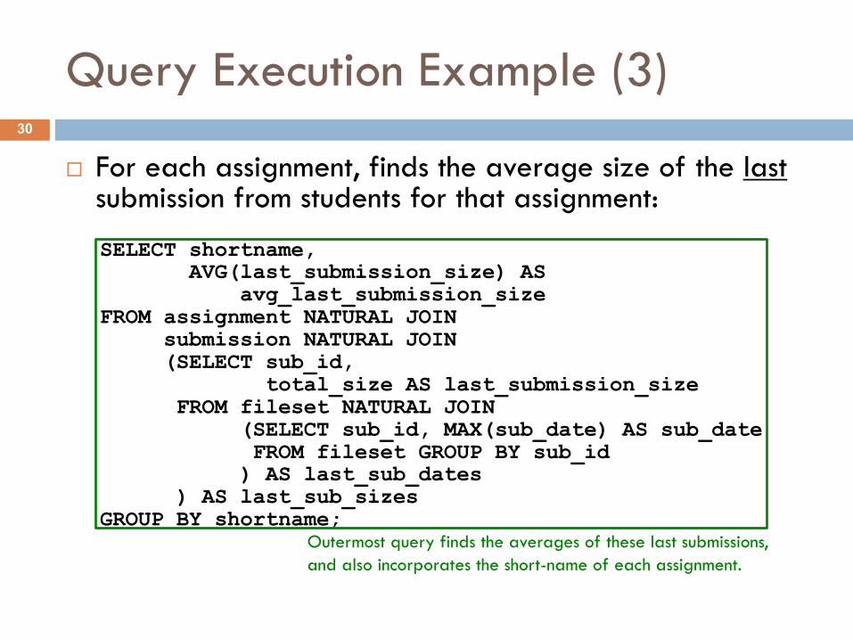
¨ For each assignment, finds the average size of the lastsubmission from students for that assignment:
SELECT shortname,AVG(last_submission_size) AS
avg_last_submission_sizeFROM assignment NATURAL JOIN
submission NATURAL JOIN(SELECT sub_id,
total_size AS last_submission_sizeFROM fileset NATURAL JOIN
(SELECT sub_id, MAX(sub_date) AS sub_dateFROM fileset GROUP BY sub_id) AS last_sub_dates
) AS last_sub_sizesGROUP BY shortname;
Find the date of the last fileset submitted for eachstudent’s submission. Name the result columns toallow a natural join against the fileset table.
28
Query Execution Example (2)
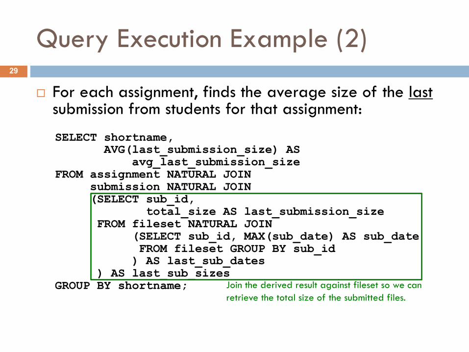
¨ For each assignment, finds the average size of the lastsubmission from students for that assignment:
SELECT shortname,AVG(last_submission_size) AS
avg_last_submission_sizeFROM assignment NATURAL JOIN
submission NATURAL JOIN(SELECT sub_id,
total_size AS last_submission_sizeFROM fileset NATURAL JOIN
(SELECT sub_id, MAX(sub_date) AS sub_dateFROM fileset GROUP BY sub_id) AS last_sub_dates
) AS last_sub_sizesGROUP BY shortname; Join the derived result against fileset so we can
retrieve the total size of the submitted files.
29
Query Execution Example (3)
¨ For each assignment, finds the average size of the lastsubmission from students for that assignment:
SELECT shortname,AVG(last_submission_size) AS
avg_last_submission_sizeFROM assignment NATURAL JOIN
submission NATURAL JOIN(SELECT sub_id,
total_size AS last_submission_sizeFROM fileset NATURAL JOIN
(SELECT sub_id, MAX(sub_date) AS sub_dateFROM fileset GROUP BY sub_id) AS last_sub_dates
) AS last_sub_sizesGROUP BY shortname;
Outermost query finds the averages of these last submissions,and also incorporates the short-name of each assignment.
30
MySQL Execution and Analysis
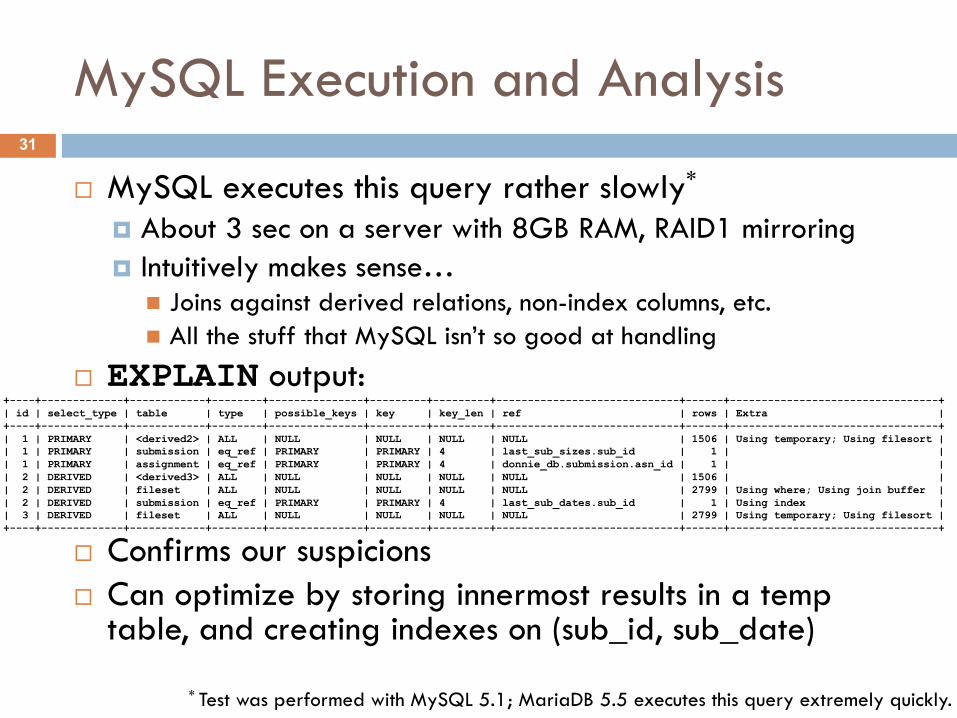
¨ MySQL executes this query rather slowly*
¤ About 3 sec on a server with 8GB RAM, RAID1 mirroring¤ Intuitively makes sense…
n Joins against derived relations, non-index columns, etc.n All the stuff that MySQL isn’t so good at handling
¨ EXPLAIN output:
¨ Confirms our suspicions¨ Can optimize by storing innermost results in a temp
table, and creating indexes on (sub_id, sub_date)
+----+-------------+------------+--------+---------------+---------+---------+-----------------------------+------+---------------------------------+| id | select_type | table | type | possible_keys | key | key_len | ref | rows | Extra |+----+-------------+------------+--------+---------------+---------+---------+-----------------------------+------+---------------------------------+| 1 | PRIMARY | <derived2> | ALL | NULL | NULL | NULL | NULL | 1506 | Using temporary; Using filesort | | 1 | PRIMARY | submission | eq_ref | PRIMARY | PRIMARY | 4 | last_sub_sizes.sub_id | 1 | | | 1 | PRIMARY | assignment | eq_ref | PRIMARY | PRIMARY | 4 | donnie_db.submission.asn_id | 1 | | | 2 | DERIVED | <derived3> | ALL | NULL | NULL | NULL | NULL | 1506 | | | 2 | DERIVED | fileset | ALL | NULL | NULL | NULL | NULL | 2799 | Using where; Using join buffer | | 2 | DERIVED | submission | eq_ref | PRIMARY | PRIMARY | 4 | last_sub_dates.sub_id | 1 | Using index | | 3 | DERIVED | fileset | ALL | NULL | NULL | NULL | NULL | 2799 | Using temporary; Using filesort | +----+-------------+------------+--------+---------------+---------+---------+-----------------------------+------+---------------------------------+
* Test was performed with MySQL 5.1; MariaDB 5.5 executes this query extremely quickly.
31
PostgreSQL Execution/Analysis (1)
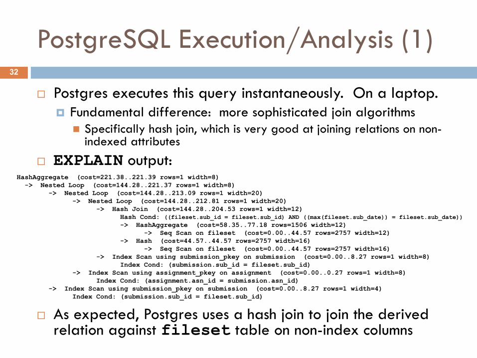
¨ Postgres executes this query instantaneously. On a laptop.¤ Fundamental difference: more sophisticated join algorithms
n Specifically hash join, which is very good at joining relations on non-indexed attributes
¨ EXPLAIN output:
¨ As expected, Postgres uses a hash join to join the derived relation against fileset table on non-index columns
HashAggregate (cost=221.38..221.39 rows=1 width=8)-> Nested Loop (cost=144.28..221.37 rows=1 width=8)
-> Nested Loop (cost=144.28..213.09 rows=1 width=20)-> Nested Loop (cost=144.28..212.81 rows=1 width=20)
-> Hash Join (cost=144.28..204.53 rows=1 width=12)Hash Cond: ((fileset.sub_id = fileset.sub_id) AND ((max(fileset.sub_date)) = fileset.sub_date))-> HashAggregate (cost=58.35..77.18 rows=1506 width=12)
-> Seq Scan on fileset (cost=0.00..44.57 rows=2757 width=12)-> Hash (cost=44.57..44.57 rows=2757 width=16)
-> Seq Scan on fileset (cost=0.00..44.57 rows=2757 width=16)-> Index Scan using submission_pkey on submission (cost=0.00..8.27 rows=1 width=8)
Index Cond: (submission.sub_id = fileset.sub_id)-> Index Scan using assignment_pkey on assignment (cost=0.00..0.27 rows=1 width=8)
Index Cond: (assignment.asn_id = submission.asn_id)-> Index Scan using submission_pkey on submission (cost=0.00..8.27 rows=1 width=4)
Index Cond: (submission.sub_id = fileset.sub_id)
32
PostgreSQL Execution/Analysis (2)
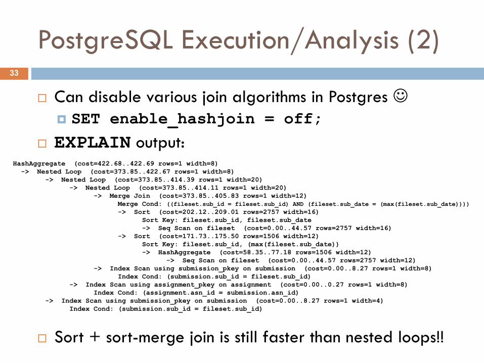
¨ Can disable various join algorithms in Postgres J¤ SET enable_hashjoin = off;
¨ EXPLAIN output:
¨ Sort + sort-merge join is still faster than nested loops!!
HashAggregate (cost=422.68..422.69 rows=1 width=8)-> Nested Loop (cost=373.85..422.67 rows=1 width=8)
-> Nested Loop (cost=373.85..414.39 rows=1 width=20)-> Nested Loop (cost=373.85..414.11 rows=1 width=20)
-> Merge Join (cost=373.85..405.83 rows=1 width=12)Merge Cond: ((fileset.sub_id = fileset.sub_id) AND (fileset.sub_date = (max(fileset.sub_date))))-> Sort (cost=202.12..209.01 rows=2757 width=16)
Sort Key: fileset.sub_id, fileset.sub_date-> Seq Scan on fileset (cost=0.00..44.57 rows=2757 width=16)
-> Sort (cost=171.73..175.50 rows=1506 width=12)Sort Key: fileset.sub_id, (max(fileset.sub_date))-> HashAggregate (cost=58.35..77.18 rows=1506 width=12)
-> Seq Scan on fileset (cost=0.00..44.57 rows=2757 width=12)-> Index Scan using submission_pkey on submission (cost=0.00..8.27 rows=1 width=8)
Index Cond: (submission.sub_id = fileset.sub_id)-> Index Scan using assignment_pkey on assignment (cost=0.00..0.27 rows=1 width=8)
Index Cond: (assignment.asn_id = submission.asn_id)-> Index Scan using submission_pkey on submission (cost=0.00..8.27 rows=1 width=4)
Index Cond: (submission.sub_id = fileset.sub_id)
33
PostgreSQL Execution/Analysis (3)
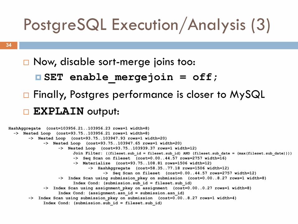
¨ Now, disable sort-merge joins too:¤ SET enable_mergejoin = off;
¨ Finally, Postgres performance is closer to MySQL¨ EXPLAIN output:
HashAggregate (cost=103956.21..103956.23 rows=1 width=8)-> Nested Loop (cost=93.75..103956.21 rows=1 width=8)
-> Nested Loop (cost=93.75..103947.93 rows=1 width=20)-> Nested Loop (cost=93.75..103947.65 rows=1 width=20)
-> Nested Loop (cost=93.75..103939.37 rows=1 width=12)Join Filter: ((fileset.sub_id = fileset.sub_id) AND (fileset.sub_date = (max(fileset.sub_date))))-> Seq Scan on fileset (cost=0.00..44.57 rows=2757 width=16)-> Materialize (cost=93.75..108.81 rows=1506 width=12)
-> HashAggregate (cost=58.35..77.18 rows=1506 width=12)-> Seq Scan on fileset (cost=0.00..44.57 rows=2757 width=12)
-> Index Scan using submission_pkey on submission (cost=0.00..8.27 rows=1 width=8)Index Cond: (submission.sub_id = fileset.sub_id)
-> Index Scan using assignment_pkey on assignment (cost=0.00..0.27 rows=1 width=8)Index Cond: (assignment.asn_id = submission.asn_id)
-> Index Scan using submission_pkey on submission (cost=0.00..8.27 rows=1 width=4)Index Cond: (submission.sub_id = fileset.sub_id)
34
Query Estimates
¨ Query planner/optimizer must make estimates about the cost of each stage
¨ Database maintains statistics for each table, to facilitate planning and optimization
¨ Different levels of detail:¤ Some DBs only track min/max/count of values in each column.
Estimates are very basic.¤ Some DBs generate and store histograms of values in important
columns. Estimates are much more accurate.¨ Different levels of accuracy:
¤ Statistics are expensive to maintain! Databases update these statistics relatively infrequently.
¤ If a table’s contents change substantially, must recompute statistics
35
Table Statistics Analysis
¨ Databases also frequently provide a command to compute table statistics
¨ MySQL command:ANALYZE TABLE assignment, submission, fileset;
¨ PostgreSQL command:VACUUM ANALYZE;
n for all tables in databaseVACUUM ANALYZE tablename;
n for a specific table¨ These commands are expensive!
¤ Perform a full table-scan¤ Also, typically lock the table(s) for exclusive access
36
Review
¨ Discussed general details of how most databases evaluate SQL queries
¨ Some relational algebra operations have several ways to evaluate them¤ Optimizations for very common special cases, e.g.
equijoins¨ Can give the database some guidance
¤ Create indexes on tables where appropriate¤ Rewrite queries to be more efficient¤ Make sure statistics are up-to-date, so that planner has
best chance of generating a good plan
37

![Microsoft SQL Server Query Tuning - Meetupfiles.meetup.com/1381968/Microsoft SQL Server Query...Microsoft PowerPoint - Microsoft SQL Server Query Tuning [Compatibility Mode] Author](https://img.pdfslide.us/doc/110x75/5ad9c9447f8b9afc0f8b9e56/microsoft-sql-server-query-tuning-sql-server-querymicrosoft-powerpoint-microsoft.jpg)