Embed Size (px)
DESCRIPTION
Analysis of Deadline Scheduled Real Time Systems
Citation preview
ISS
N 0
249-
6399
appor t de r echerche
INSTITUT NATIONAL DE RECHERCHE EN INFORMATIQUE ET EN AUTOMATIQUE
Analysis of Deadline Scheduled Real-TimeSystems
Marco Spuri
N˚ 2772Janvier 1996
PROGRAMME 1

Analysis of Deadline Scheduled Real-Time Systems
Marco Spuri �
Programme 1 | Architectures parall�eles, bases de donn�ees, r�eseaux et syst�emes distribu�esProjet Re ecs
Rapport de recherche n�2772 | Janvier 1996 | 31 pages
Abstract: A uniform, exible approach is proposed for analysing the feasibility of deadlinescheduled real-time systems. In its most general formulation, the analysis assumes sporad-ically periodic tasks with arbitrary deadlines, release jitter, and shared resources. Systemoverheads of a tick driven scheduler implementation, and scheduling of soft aperiodic tasksare also accounted for.
A procedure for the computation of task worst-case response times is also described forthe same model. While this problem has been largely studied in the context of �xed prioritysystems, we are not aware of other works that have proposed a solution to it when deadlinescheduling is assumed. The worst-case response time evaluation is a fundamental tool foranalysing end-to-end timing constraints in distributed systems [21].
Key-words: real-time, scheduling, feasibility analysis, response times.
(R�esum�e : tsvp)
�This work has been supported by the Commission of the European Communities under contractERBCHBGCT930458, proposal ERB4050PL931117.
Unité de recherche INRIA RocquencourtDomaine de Voluceau, Rocquencourt, BP105, 78153 LE CHESNAY Cedex (France)
Téléphone : (33 1) 39 63 55 11 – Télécopie : (33 1) 39 63 53 30
Analyse de Syst�emes Temps-R�eel �a Ordonnancement
par �Ech�eance la plus Proche en Premier
R�esum�e : Une technique uniforme et exible est propos�ee pour analyser la faisabilit�e desyst�emes temps-r�eel �a ordonnancement par �ech�eance la plus proche en premier (EDF). Danssa formulation la plus g�en�erale, l'analyse consid�ere des taches sporadiquement p�eriodiques�a �ech�eances arbitraires, �a jigues sur les instants d'activation, et avec partage de ressources.Les couts induits par l'ordonnancement des taches ap�eriodiques (�a �ech�eances non strictes)et par une implantation bas�ee sur une horloge sont pris en compte.
Une proc�edure pour le calcul du pire temps de r�eponse des taches est d�ecrite pour lemod�ele consid�er�e. Bien que ce probl�eme ait d�ej�a �et�e �etudi�e pour des syst�emes �a priorit�es �xes,nous ne connaissons aucun travail sur ce sujet lorsque l'ordonnancement EDF est utilis�e.L'�evaluation des pires temps de r�eponse est fondamentale pour l'analyse de contraintestemporelles de bout-en-bout dans les syst�emes distribu�es [21].
Mots-cl�e : temps-r�eel, ordonnancement, analyse de faisabilit�e, temps de r�eponse.
Analysis of Deadline Scheduled Real-Time Systems 3
1 Introduction
Real-time systems are characterized by tasks with stringent timing constraints, that mustbe met in order to guarantee correctness and safety. One of the main issues of such systemsis predictability. Central to this issue is the study of suitable scheduling algorithms thatlet us analyse a priori the feasibility of the system, that is, establish whether the timingconstraints are going to be met or there are potential failures, before the system is actuallybuilt.
Within uniprocessor systems, two well known algorithms, Rate Monotonic and EarliestDeadline First (EDF), have been shown optimal with respect to �xed and dynamic prioritypre-emptive schemes, in the fundamental work of Liu and Layland [11]. In this work, thetwo algorithms were studied under a number of restrictions, among which:
� all tasks were strictly periodic;
� deadlines were equal to periods;
� all tasks were independent.
Later, several papers have appeared in the literature in order to extend the analysis of Liuand Layland to more general and useful models. Suitable concurrency control protocols [2,4, 14] have been proposed for handling shared resources. Tasks have been allowed to havedeadlines shorter than their periods [1, 3, 9]. Aperiodic scheduling has also received muchattention [6, 8, 10, 15, 16, 17].
Quite recently, Tindell et al. [20] presented further extensions to the existing theory foranalysing �xed priority pre-emptive systems. The major contributions of their approach are
� arbitrary deadlines (i.e. deadlines may also be greater than periods),
� periodic and sporadic tasks,
� release jitter (a delay between the arrival and the actual release of a task instance),
� `bursty' tasks.
A very interesting aspect of their approach is that the analysis is entirely based on thecomputation of task worst-case response times. This computation not only is importantfor assessing the feasibility of a uniprocessor system, but it also plays a fundamental rolewhen we extend our attention to real-time distributed systems. Distributed applicationsare characterized by precedence relationships between their tasks. If the tasks are staticallyallocated to single processors, end-to-end timing constraints can be analysed by a theorywhich assumes release jitter [1]: \All tasks are de�ned to arrive at the same time, but aprecedence constrained task on one processor can have its release delayed awaiting the arrivalof a message from its predecessors. The worst-case release jitter of such a subtask can becomputed by knowing the response times of predecessor tasks located on other processors."See [22, 21] for a general treatment.
RR n�2772
4 Marco Spuri
In this paper, we focus our attention on deadline scheduled systems, and we proposea exible approach for analysing such systems, which extends previous results in a verysimilar way. The motivations of our research are that EDF scheduling always achieves higherprocessor utilization than �xed priority scheduling, and that we believe a suitable analysiscan be developed for analysing end-to-end timing constraints also when EDF scheduling islocally used in each single processor, and even in the network protocol.
Another reason for which we believe EDF scheduling should be seriously considered as acandidate for actual real-time systems is that on the contrary to Rate Monotonic, or even tothe more general Deadline Monotonic, which have shown not to be optimal when arbitrarydeadlines are assumed [9], EDF scheduling stays optimal indeed. By means of a simpleinterchange argument, Dertouzos [5] proved that any feasible pre-emptive schedule can beeasily transformed into an EDF pre-emptive schedule without a�ecting its feasibility.
Hence, similarly to [20], our goal is then to examine complex systems with sporadicallyperiodic tasks (i.e. bursty tasks), which can have arbitrary deadlines as well as arbitrary re-lease jitter, and can share resources by locking and unlocking semaphores through a suitableconcurrency control protocol. Overheads of tick driven schedulers and servers for aperiodicrequests are also considered. The analysis is based on the concept of busy period, an intervalof time in which the processor is kept busy, and simple extensions of the original Liu andLayland's theory [11]. The resulting feasibility analysis is then a generalization of some ofthe results described in [3].
Moreover, in our analysis we do not deal merely with feasibility assessment, but wealso describe a procedure for the computation of the task worst-case response times underdeadline scheduling. As already stated, the solution to this problem is a fundamental toolfor the so called holistic schedulability analysis for distributed real-time systems [21]: \Therelease jitter of a message depends on the worst-case response time of the sender task. Theworst-case response time of a task depends, in part, on the response times of messages. Amessage response time depends on its release jitter [22]."
We believe that the holistic analysis can now also be extended to distributed systemswith local EDF schedulers, even if this is the subject of current research and it will not befurther treated in this paper. We are also not aware of other works dealing with the problemof response time evaluation under EDF scheduling. That is why we believe that the majorcontribution of our work is the solution to this problem.
The paper is organized as follows. In Section 2 the notation and the assumptions usedthroughout the paper are described. The basic feasibility analysis for periodic and sporadictask sets with arbitrary deadlines is treated in Section 3, while in Section 4 we describethe procedure for the computation of worst-case response times under the same model.Sections 5, 6, 7, 8, and 9, deal with several extensions to the basic model: release jit-ter, sporadically periodic tasks, resource sharing, inclusion of soft aperiodic tasks, and tickscheduling overheads, respectively. In all extensions, both the feasibility analysis and theworst-case response time computation are treated in detail. A case study is presented inSection 10. Finally, our conclusions are stated in Section 11. In Appendix A we have repor-ted the prooves of a couple of properties concerning the busy period analysis which we do
INRIA
Analysis of Deadline Scheduled Real-Time Systems 5
not consider essential for the comprehension of the paper. Furthermore, in Appendix B thecomplete description of our analysis is summarized.
2 Computational Model and Notation
This work is mainly inspired by the results presented in [1, 20]. Our goal is to �nd anapproach for the analysis of problems similar to those studied there, in which the basicassumption of �xed priority pre-emptive scheduling is replaced by the assumption of EDFpre-emptive scheduling. More speci�cally, we assume the same processor workload model,i.e. task arrival laws and properties, while the scheduling mechanism is now deadline-based:at any time, the ready task with the earliest deadline is run. For this reason, we also adopt,as far as possible, the same notation as in [1, 20].
In the paper we consider the scheduling of tasks on a single processor. A task consists ofan in�nite number of requests, or instances, whose arrival times are separated by a minimumtime T , called period (according to the conventional notation, this assumption is commonto periodic and sporadic tasks). We assume that task instances may arrive at any time.However, the arrival must be recognized by a run-time dispatcher, which then will place theinstance in a notional run-time queue. The instance is then said to be released. The timebetween a task's arrival and its release1 is known as release jitter.
Each task instance may execute for a bounded amount of computation C, called worst-case execution time. The computation should complete within a time D (relative deadline)after the arrival. The notional run-queue is ordered according to the actual task's deadlines,earliest �rst, that is, we assume an EDF [11] pre-emptive dispatching. Tasks may also shareresources, by locking and unlocking semaphores according to a protocol like the PriorityCeiling [14, 4] or the Stack Resource Policy [2].
In a later section we also extend the workload model with the so called sporadicallyperiodic tasks [1]. This sort of tasks is intended to model the behaviour of events whichmay arrive at a certain rate for a number of times, and then not re-arrive for a longer time.For example, there are interrupts which behave in this way (they are also termed burstysporadics). Sporadically periodic tasks are assigned two periods: an inner period (t) andan outer period (T ). The outer period is the worst-case inter-arrival time between bursts.The inner period is the worst-case inter-arrival time between task instances within a burst.There is a bounded number of arrivals to each burst. Furthermore, the total time for theburst (i.e. the number of inner arrivals multiplied by the inner period) must be less than orequal to the outer period. A task that is not a bursty task is simply modelled as one thathas an inner period equal to the outer period, and at most one inner arrival.
A glossary of the notation used in this paper follows:
Ci The worst-case computation time of task i on each release.
Di The deadline of task i, measured relative to the arrival time of the task.
1Note that the release of a task can also be delayed by other factors, such as a distributed synchronization.
RR n�2772
6 Marco Spuri
Bi The worst-case blocking time task i can experience due to the operation of the concur-rency control protocol.
Ji The worst-case release jitter of task i (i.e. the worst-case delay between the arrivaland its release).
Ti The outer period of task i.
ti The inner period of task i.
ni The worst-case number of arrivals of task i per outer period.
ri The worst-case response time of task i, measured from the arrival time to the comple-tion time.
Ii(t) The number of instances of task i released before time t.
Hi(t) The number of instances of task i with deadline before or at t.
si(a) The release time of the �rst instance of task i, in an arrival pattern where another i'sinstance arrives at time a.
L The length of the �rst busy period in the most demanding arrival pattern.
US The processor utilization allocated to the aperiodic server.
3 Basic Feasibility Analysis
In this section, as well as in the following one, we assume a simple model in which all taskshave null release jitter, do not share resources, and are not bursty (i.e. 8i; Ji = 0; Bi =0; ti = Ti; ni = 1). A basic feasibility analysis is presented and is later extended to handlemore general models.
Given a task set, according to the assumptions, we can have di�erent patterns of arrivals(recall that the period is only a worst-case inter-arrival time). It is not di�cult to show thatthe worst-case pattern is that in which the task instances are released as soon as possible,that is, the �rst instance is released at time t = 0, and the others are then released accordingto the task's period (this pattern is termed asap in the rest of this paper). The result isquite intuitive, and it can be proven using the same argument as in Theorem 6 of the wellknown work by Liu and Layland [11].
Theorem 3.1 (Liu and Layland) When the deadline driven scheduling algorithm is usedto schedule a set of tasks on a processor, if there is an over ow for a certain arrival pattern,then there is an over ow without idle time prior to it in the pattern in which all task instancesare released as soon as possible (i.e. in the asap arrival pattern).
INRIA
Analysis of Deadline Scheduled Real-Time Systems 7
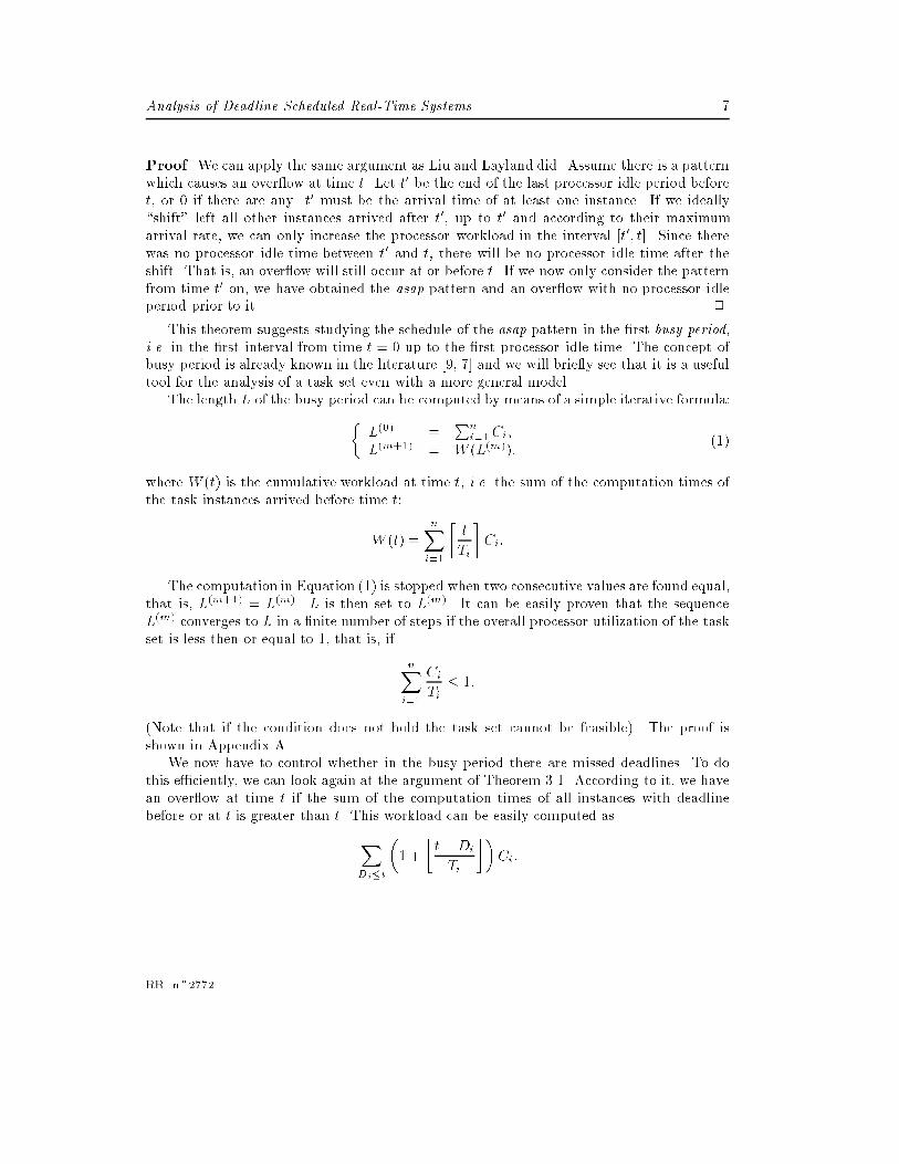
Proof. We can apply the same argument as Liu and Layland did. Assume there is a patternwhich causes an over ow at time t. Let t0 be the end of the last processor idle period beforet, or 0 if there are any. t0 must be the arrival time of at least one instance. If we ideally\shift" left all other instances arrived after t0, up to t0 and according to their maximumarrival rate, we can only increase the processor workload in the interval [t0; t]. Since therewas no processor idle time between t0 and t, there will be no processor idle time after theshift. That is, an over ow will still occur at or before t. If we now only consider the patternfrom time t0 on, we have obtained the asap pattern and an over ow with no processor idleperiod prior to it. 2
This theorem suggests studying the schedule of the asap pattern in the �rst busy period,i.e. in the �rst interval from time t = 0 up to the �rst processor idle time. The concept ofbusy period is already known in the literature [9, 7] and we will brie y see that it is a usefultool for the analysis of a task set even with a more general model.
The length L of the busy period can be computed by means of a simple iterative formula:�L(0) =
Pn
i=1Ci;
L(m+1) = W (L(m));(1)
where W (t) is the cumulative workload at time t, i.e. the sum of the computation times ofthe task instances arrived before time t:
W (t) =nXi=1
�t
Ti
�Ci:
The computation in Equation (1) is stopped when two consecutive values are found equal,that is, L(m+1) = L(m). L is then set to L(m). It can be easily proven that the sequenceL(m) converges to L in a �nite number of steps if the overall processor utilization of the taskset is less then or equal to 1, that is, if
nXi=1
Ci
Ti� 1:
(Note that if the condition does not hold the task set cannot be feasible). The proof isshown in Appendix A.
We now have to control whether in the busy period there are missed deadlines. To dothis e�ciently, we can look again at the argument of Theorem 3.1. According to it, we havean over ow at time t if the sum of the computation times of all instances with deadlinebefore or at t is greater than t. This workload can be easily computed as
XDi�t
�1 +
�t�Di
Ti
��Ci:
RR n�2772
8 Marco Spuri
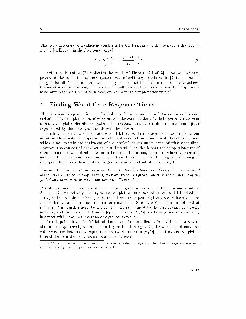
That is, a necessary and su�cient condition for the feasibility of the task set is that for allactual deadlines d in the �rst busy period
d �XDi�d
�1 +
�d�Di
Ti
��Ci: (2)
Note that Equation (2) replicates the result of Theorem 3.1 of [3]. However, we havepresented the result in the more general case of arbitrary deadlines (in [3] it is assumedDi � Ti for all i). Furthermore, we not only believe that the argument used here to achievethe result is quite intuitive, but as we will brie y show, it can also be used to compute themaximum response time of each task, even in a more complex framework.2
4 Finding Worst-Case Response Times
The worst-case response time ri of a task i is the maximum time between an i's instancearrival and its completion. As already stated, the computation of ri is important if we wantto analyse a global distributed system: the response time of a task is the maximum jitterexperienced by the messages it sends over the network.
Finding ri is not a trivial task when EDF scheduling is assumed. Contrary to ourintuition, the worst-case response time of a task is not always found in the �rst busy period,which is not exactly the equivalent of the critical instant under �xed priority scheduling.However, the concept of busy period is still useful. The idea is that the completion time ofa task's instance with deadline d, must be the end of a busy period in which all executedinstances have deadlines less than or equal to d. In order to �nd the longest one among allsuch periods, we can then apply an argument similar to that of Theorem 3.1.
Lemma 4.1 The worst-case response time of a task i is found in a busy period in which allother tasks are released asap, that is, they are released synchronously at the beginning of theperiod and then at their maximum rate (see Figure 1b).
Proof. Consider a task i's instance, like in Figure 1a, with arrival time a and deadlined = a + Di, respectively. Let t2 be its completion time, according to the EDF schedule.Let t1 be the last time before t2, such that there are no pending instances with arrival timeearlier than t1 and deadline less than or equal to d. Since the i's instance is released att = a, t1 � a. Furthermore, by choice of t1 and t2, t1 must be the arrival time of a task'sinstance, and there is no idle time in [t1; t2]. That is, [t1; t2] is a busy period in which onlyinstances with deadlines less than or equal to d execute.
At this point, if we \shift" left all instances of tasks di�erent from i, in such a way toobtain an asap arrival pattern, like in Figure 1b, starting at t1, the workload of instanceswith deadlines less than or equal to d cannot diminish in [t1; t2]. That is, the completiontime of the i's instance considered can only increase. 2
2In [17], a similar technique is used to build a more realistic analysis in which both the system overheadsand the interrupt handling are taken into account.
INRIA
Analysis of Deadline Scheduled Real-Time Systems 9
OtherTasks
1 2
(a)
iTask
(b)
0
t a t d t
a d t
t
t
t
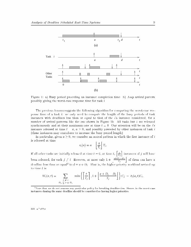
Figure 1: a) Busy period preceding an instance completion time. b) Asap arrival patternpossibly giving the worst-case response time for task i.
The previous lemma suggests the following algorithm for computing the worst-case res-ponse time of a task i: we only need to compute the length of the busy periods of taskinstances with deadlines less than or equal to that of the i's instance considered, for anumber of arrival patterns like the one shown in Figure 1b. All tasks but i are releasedsynchronously and at their maximum rate at time t = 0. Our attention will be on the i'sinstance released at time t = a, a � 0, and possibly preceded by other instances of task i
(these instances may contribute to increase the busy period length).In particular, given a � 0, we consider an arrival pattern in which the �rst instance of i
is released at time
si(a) = a�
�a
Ti
�Ti:
If all other tasks are initially released at time t = 0, at time t,ltTj
minstances of j will have
been released, for each j 6= i. However, at most only 1 +ja+Di�Dj
Tj
kof them can have a
deadline less than or equal3 to d = a+Di. That is, the higher priority workload arrived upto time t is
Wi(a; t) =Xj 6= i
Dj � a +Di
min
��t
Tj
�; 1 +
�a+Di �Dj
Tj
��Cj + �i(a; t)Ci;
3Note that we do not assume any particular policy for breaking deadline ties. Hence, in the worst-caseinstances sharing the same deadline should be considered as having higher priorities.
RR n�2772
10 Marco Spuri
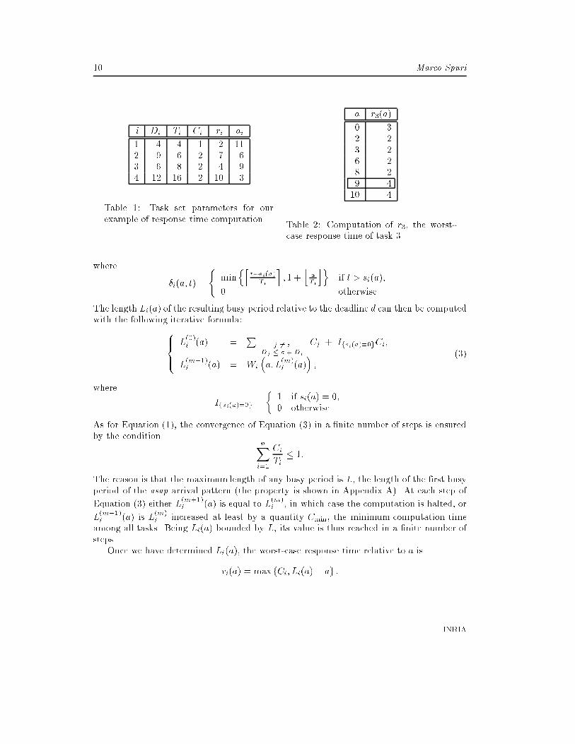
i Di Ti Ci ri ai
1 4 4 1 2 112 9 6 2 7 63 6 8 2 4 94 12 16 2 10 3
Table 1: Task set parameters for ourexample of response time computation.
a r3(a)
0 32 23 26 28 29 410 4
Table 2: Computation of r3, the worst-case response time of task 3.
where
�i(a; t) =
(min
nlt�si(a)
Ti
m; 1 +
jaTi
koif t > si(a),
0 otherwise.
The length Li(a) of the resulting busy period relative to the deadline d can then be computedwith the following iterative formula:8><
>:L(0)i (a) =
Pj 6= i
Dj � a+ Di
Cj + Ifsi(a)=0gCi;
L(m+1)i (a) = Wi
�a; L
(m)i (a)
�;
(3)
where
Ifsi(a)=0g =
�1 if si(a) = 0,0 otherwise.
As for Equation (1), the convergence of Equation (3) in a �nite number of steps is ensuredby the condition
nXi=1
Ci
Ti� 1:
The reason is that the maximum length of any busy period is L, the length of the �rst busyperiod of the asap arrival pattern (the property is shown in Appendix A). At each step of
Equation (3) either L(m+1)i (a) is equal to L
(m)i , in which case the computation is halted, or
L(m+1)i (a) is L
(m)i increased at least by a quantity Cmin, the minimum computation time
among all tasks. Being Li(a) bounded by L, its value is thus reached in a �nite number ofsteps.
Once we have determined Li(a), the worst-case response time relative to a is
ri(a) = maxfCi; Li(a)� ag :
INRIA
Analysis of Deadline Scheduled Real-Time Systems 11
OtherTasks
Taskt
3
t
t
t0
a=9s (a)=1 d=153
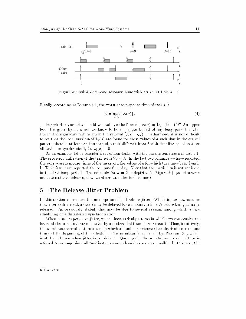
Figure 2: Task 3 worst-case response time with arrival at time a = 9.
Finally, according to Lemma 4.1, the worst-case response time of task i is
ri = maxa�0
fri(a)g : (4)
For which values of a should we evaluate the function ri(a) in Equation (4)? An upperbound is given by L, which we know to be the upper bound of any busy period length.Hence, the signi�cant values are in the interval [0; L� Ci). Furthermore, it is not di�cultto see that the local maxima of Li(a) are found for those values of a such that in the arrivalpattern there is at least an instance of a task di�erent from i with deadline equal to d, orall tasks are synchronized, i.e. si(a) = 0.
As an example, let us consider a set of four tasks, with the parameters shown in Table 1.The processor utilization of the task set is 95.83%. In the last two columns we have reportedthe worst-case response times of the tasks and the values of a for which they have been found.In Table 2 we have reported the computation of r3. Note that the maximum is not achievedin the �rst busy period. The schedule for a = 9 is depicted in Figure 2 (upward arrowsindicate instance releases, downward arrows indicate deadlines).
5 The Release Jitter Problem
In this section we remove the assumption of null release jitter. Which is, we now assumethat after each arrival, a task i may be delayed for a maximum time Ji before being actuallyreleased. As previously stated, this may be due to several reasons among which a tickscheduling or a distributed synchronization.
When a task experiences jitter, we can have arrival patterns in which two consecutive re-leases of the same task are separated by an interval of time shorter than T . Thus, intuitively,the worst-case arrival pattern is one in which all tasks experience their shortest inter-releasetimes at the beginning of the schedule. This intuition is con�rmed by Theorem 3.1, whichis still valid even when jitter is considered. Once again, the worst-case arrival pattern isreferred to as asap, since all task instances are released as soon as possible. In this case, the
RR n�2772
12 Marco Spuri
0
1
3
1
2
3
-J
-J
-JT
T
t
t
t
T2
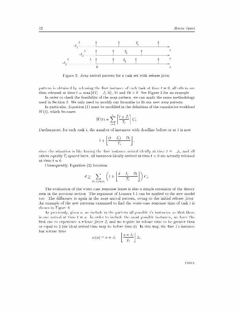
Figure 3: Asap arrival pattern for a task set with release jitter.
pattern is obtained by releasing the �rst instance of each task at time t = 0, all others arethen released at time t = maxfkTi � Ji; 0g, 8i and 8k > 0. See Figure 3 for an example.
In order to check the feasibility of the asap pattern, we can apply the same methodologyused in Section 3. We only need to modify our formulae to �t our new asap pattern.
In particular, Equation (1) must be modi�ed in the de�nition of the cumulative workloadW (t), which becomes
W (t) =nXi=1
�t+ Ji
Ti
�Ci:
Furthermore, for each task i, the number of instances with deadline before or at t is now
1 +
�(t+ Ji) �Di
Ti
�;
since the situation is like having the �rst instance arrival ideally at time t = �Ji, and allothers equally Ti spaced later: all instances ideally arrived at time t < 0 are actually releasedat time t = 0.
Consequently, Equation (2) becomes
d �X
Di�d+Ji
�1 +
�d+ Ji �Di
Ti
��Ci:
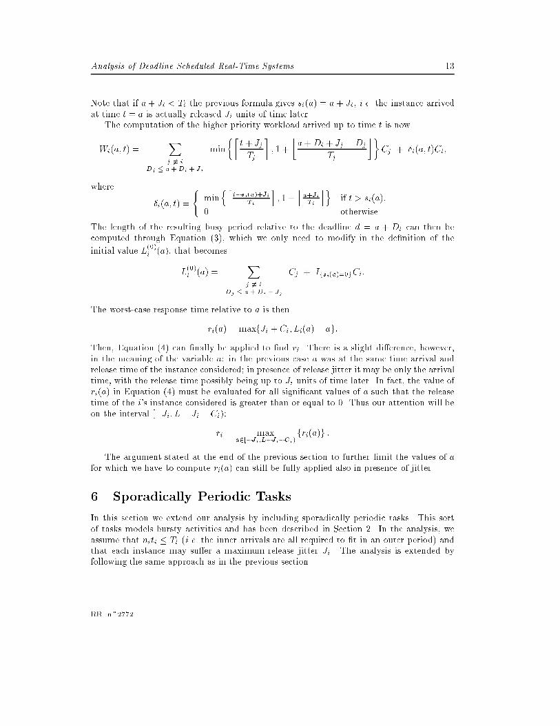
The evaluation of the worst-case response times is also a simple extension of the theoryseen in the previous section. The argument of Lemma 4.1 can be applied to the new modeltoo. The di�erence is again in the asap arrival pattern, owing to the initial release jitter.An example of the new patterns examined to �nd the worst-case response time of task i isshown in Figure 4.
As previously, given a, we include in the pattern all possible i's instances, so that thereis one arrival at time t = a. In order to include the most possible instances, we force the�rst one to experience a release jitter Ji and we require its release time to be greater thanor equal to 0 (its ideal arrival time may be before time 0). In this way, the �rst i's instancehas release time
si(a) = a+ Ji �
�a+ Ji
Ti
�Ti:
INRIA
Analysis of Deadline Scheduled Real-Time Systems 13
Note that if a+ Ji < Ti the previous formula gives si(a) = a + Ji, i.e. the instance arrivedat time t = a is actually released Ji units of time later.
The computation of the higher priority workload arrived up to time t is now
Wi(a; t) =Xj 6= i
Dj � a+Di + Jj
min
��t + Jj
Tj
�; 1 +
�a+Di + Jj �Dj
Tj
��Cj + �i(a; t)Ci;
where
�i(a; t) =
(min
nlt�si(a)+Ji
Ti
m; 1 +
ja+JiTi
koif t > si(a),
0 otherwise.
The length of the resulting busy period relative to the deadline d = a + Di can then becomputed through Equation (3), which we only need to modify in the de�nition of the
initial value L(0)i (a), that becomes
L(0)i (a) =
Xj 6= i
Dj � a +Di + Jj
Cj + Ifsi(a)=0gCi:
The worst-case response time relative to a is then
ri(a) = maxfJi + Ci; Li(a) � ag:
Then, Equation (4) can �nally be applied to �nd ri. There is a slight di�erence, however,in the meaning of the variable a: in the previous case a was at the same time arrival andrelease time of the instance considered; in presence of release jitter it may be only the arrivaltime, with the release time possibly being up to Ji units of time later. In fact, the value ofri(a) in Equation (4) must be evaluated for all signi�cant values of a such that the releasetime of the i's instance considered is greater than or equal to 0. Thus our attention will beon the interval [�Ji; L� Ji �Ci):
ri = maxa2[�Ji;L�Ji�Ci)
fri(a)g :
The argument stated at the end of the previous section to further limit the values of afor which we have to compute ri(a) can still be fully applied also in presence of jitter.
6 Sporadically Periodic Tasks
In this section we extend our analysis by including sporadically periodic tasks. This sortof tasks models bursty activities and has been described in Section 2. In the analysis, weassume that niti � Ti (i.e. the inner arrivals are all required to �t in an outer period) andthat each instance may su�er a maximum release jitter Ji. The analysis is extended byfollowing the same approach as in the previous section.
RR n�2772
14 Marco Spuri
0
t
t
a tds (a)i
Ji
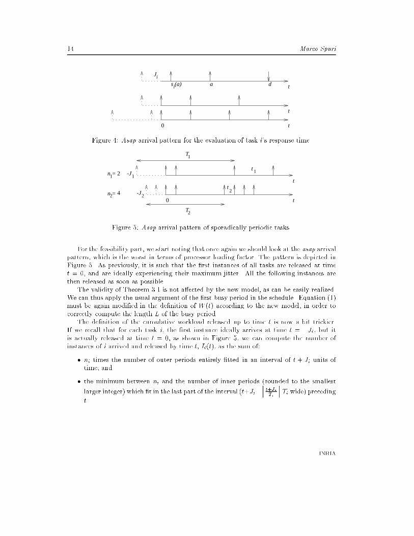
Figure 4: Asap arrival pattern for the evaluation of task i's response time.
1t
2t
T2
1T
1n = 2
2n = 4
1-Jt
2-Jt0
Figure 5: Asap arrival pattern of sporadically periodic tasks.
For the feasibility part, we start noting that once again we should look at the asap arrivalpattern, which is the worst in terms of processor loading factor. The pattern is depicted inFigure 5. As previously, it is such that the �rst instances of all tasks are released at timet = 0, and are ideally experiencing their maximum jitter. All the following instances arethen released as soon as possible.
The validity of Theorem 3.1 is not a�ected by the new model, as can be easily realized.We can thus apply the usual argument of the �rst busy period in the schedule. Equation (1)must be again modi�ed in the de�nition of W (t) according to the new model, in order tocorrectly compute the length L of the busy period.
The de�nition of the cumulative workload released up to time t is now a bit trickier.If we recall that for each task i, the �rst instance ideally arrives at time t = �Ji, but itis actually released at time t = 0, as shown in Figure 5, we can compute the number ofinstances of i arrived and released by time t, Ii(t), as the sum of:
� ni times the number of outer periods entirely �tted in an interval of t + Ji units oftime, and
� the minimum between ni and the number of inner periods (rounded to the smallest
larger integer) which �t in the last part of the interval (t+Ji�jt+JiTi
kTi wide) preceding
t.
INRIA
Analysis of Deadline Scheduled Real-Time Systems 15
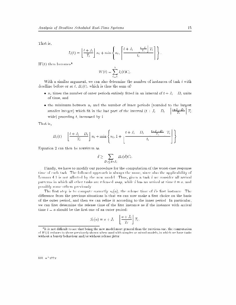
That is,
Ii(t) =
�t+ Ji
Ti
�ni +min
8<:ni;
2666t+ Ji �
jt+JiTi
kTi
ti
37779=; :
W (t) then becomes4
W (t) =nXi=1
Ii(t)Ci:
With a similar argument, we can also determine the number of instances of task i withdeadline before or at t, Hi(t), which is thus the sum of:
� ni times the number of outer periods entirely �tted in an interval of t+ Ji �Di unitsof time, and
� the minimum between ni and the number of inner periods (rounded to the largest
smaller integer) which �t in the last part of the interval (t + Ji � Di �jt+Ji�Di
Ti
kTi
wide) preceding t, increased by 1.
That is,
Hi(t) =
�t + Ji �Di
Ti
�ni +min
8<:ni; 1 +
6664 t+ Ji �Di �jt+Ji�Di
Ti
kTi
ti
77759=;
Equation 2 can then be rewritten as
d �X
Di�d+Ji
Hi(d)Ci:
Finally, we have to modify our procedure for the computation of the worst-case responsetime of each task. The followed approach is always the same, since also the applicability ofLemma 4.1 is not a�ected by the new model. Thus, given a task i we consider all arrivalpatterns in which all other tasks are released asap, while i has an arrival at time t = a, andpossibly some others previously.
The �rst step is to compute correctly si(a), the release time of i's �rst instance. Thedi�erence from the previous situations is that we can now make a �rst choice on the basisof the outer period, and then we can re�ne it according to the inner period. In particular,we can �rst determine the release time of the �rst instance as if the instance with arrivaltime t = a should be the �rst one of an outer period:
Si(a) = a+ Ji �
�a+ Ji
Ti
�Ti:
4It is not di�cult to see that being the new model more general than the previous one, the computationof W (t) reduces to those previously shown when used with simpler or mixed models, in which we have taskswithout a bursty behaviour and/or without release jitter.
RR n�2772
16 Marco Spuri
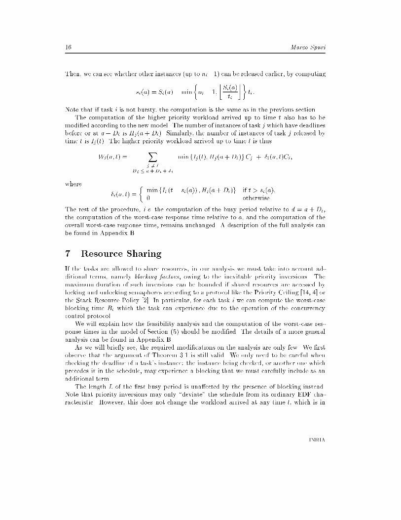
Then, we can see whether other instances (up to ni�1) can be released earlier, by computing
si(a) = Si(a)�min
�ni � 1;
�Si(a)
ti
��ti:
Note that if task i is not bursty, the computation is the same as in the previous section.The computation of the higher priority workload arrived up to time t also has to be
modi�ed according to the new model. The number of instances of task j which have deadlinesbefore or at a+Di is Hj(a +Di). Similarly, the number of instances of task j released bytime t is Ij(t). The higher priority workload arrived up to time t is thus
Wi(a; t) =Xj 6= i
Dj � a +Di + Jj
minfIj(t);Hj(a+Di)gCj + �i(a; t)Ci;
where
�i(a; t) =
�minfIi (t� si(a)) ;Hi(a+Di)g if t > si(a),0 otherwise.
The rest of the procedure, i.e. the computation of the busy period relative to d = a +Di,the computation of the worst-case response time relative to a, and the computation of theoverall worst-case response time, remains unchanged. A description of the full analysis canbe found in Appendix B.
7 Resource Sharing
If the tasks are allowed to share resources, in our analysis we must take into account ad-ditional terms, namely blocking factors, owing to the inevitable priority inversions. Themaximum duration of such inversions can be bounded if shared resources are accessed bylocking and unlocking semaphores according to a protocol like the Priority Ceiling [14, 4] orthe Stack Resource Policy [2]. In particular, for each task i we can compute the worst-caseblocking time Bi which the task can experience due to the operation of the concurrencycontrol protocol.
We will explain how the feasibility analysis and the computation of the worst-case res-ponse times in the model of Section (5) should be modi�ed. The details of a more generalanalysis can be found in Appendix B.
As we will brie y see, the required modi�cations on the analysis are only few. We �rstobserve that the argument of Theorem 3.1 is still valid. We only need to be careful whenchecking the deadline of a task's instance: the instance being checked, or another one whichprecedes it in the schedule, may experience a blocking that we must carefully include as anadditional term.
The length L of the �rst busy period is una�ected by the presence of blocking instead.Note that priority inversions may only \deviate" the schedule from its ordinary EDF cha-racteristic. However, this does not change the workload arrived at any time t, which is in
INRIA
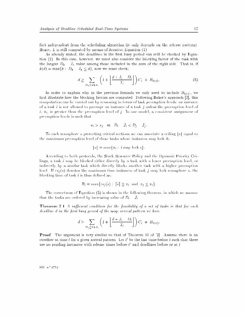
Analysis of Deadline Scheduled Real-Time Systems 17
fact independent from the scheduling algorithm (it only depends on the release pattern).Hence, L is still computed by means of iterative Equation (1).
As already stated, the deadlines in the �rst busy period can still be checked by Equa-tion (2). In this case, however, we must also consider the blocking factor of the task withthe largest Dk � Jk value among those included in the sum of the right side. That is, ifk(d) = maxfk : Dk � Jk � dg, now we must check:
d �X
Di�d+Ji
�1 +
�d+ Ji �Di
Ti
��Ci + Bk(d): (5)
In order to explain why in the previous formula we only need to include Bk(d), we�rst illustrate how the blocking factors are computed. Following Baker's approach [2], thiscomputation can be carried out by reasoning in terms of task preemption levels: an instanceof a task i is not allowed to preempt an instance of a task j unless the preemption level ofi, �i, is greater than the preemption level of j. In our model, a consistent assignment ofpreemption levels is such that
�i > �j , Di � Ji < Dj � Jj :
To each semaphore s protecting critical sections we can associate a ceiling dse equal tothe maximum preemption level of those tasks whose instances may lock it:
dse = maxf�i : i may lock sg:
According to both protocols, the Stack Resource Policy and the Dynamic Priority Cei-lings, a task i may be blocked either directly by a task with a lower preemption level, orindirectly by a similar task which directly blocks another task with a higher preemptionlevel. If csj(s) denotes the maximum time instances of task j may lock semaphore s, theblocking time of task i is thus de�ned as:
Bi = maxfcsj(s) : dse � �i and �j � �ig:
The correctness of Equation (5) is shown in the following theorem, in which we assumethat the tasks are ordered by increasing value of Di � Ji.
Theorem 7.1 A su�cient condition for the feasibility of a set of tasks is that for eachdeadline d in the �rst busy period of the asap arrival pattern we have
d �X
Di�d+Ji
�1 +
�d+ Ji �Di
Ti
��Ci + Bk(d):
Proof. The argument is very similar to that of Theorem 10 of [2]. Assume there is anover ow at time t for a given arrival pattern. Let t0 be the last time before t such that thereare no pending instances with release times before t0 and deadlines before or at t.
RR n�2772
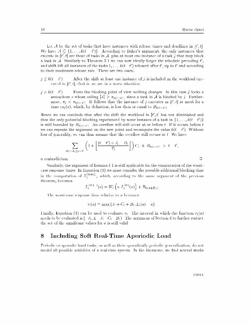
18 Marco Spuri
Let A be the set of tasks that have instances with release times and deadlines in [t0; t].We have A � f1; : : : ; k(t � t0)g. According to Baker's argument, the only instances thatexecute in [t0; t] are those of tasks in A, plus at most one instance of a task j that may blocka task in A. Similarly to Theorem 3.1 we can now ideally forget the schedule preceding t0,and shift left all instances of the tasks 1; : : : ; k(t� t0) released after t0, up to t0 and accordingto their maximum release rate. There are two cases:
j � k(t� t0) { After the shift at least one instance of j is included in the workload exe-cuted in [t0; t], that is, we are in a worse situation.
j > k(t� t0) { From the blocking point of view nothing changes. In this case j locks asemaphore s whose ceiling dse � �k(t�t0), since a task in A is blocked by j. Further-more, �j < �k(t�t0). It follows that the instance of j executes in [t0; t] at most for atime csj(s), which, by de�nition, is less then or equal to Bk(t�t0).
Hence we can conclude that after the shift the workload in [t0; t] has not diminished andthat the only potential blocking experienced by some instance of a task in f1; : : : ; k(t� t0)gis still bounded by Bk(t�t0). An over ow will still occur at or before t. If it occurs before twe can repeate the argument on the new point and recompute the value k(t� t0). Withoutloss of generality, we can thus assume that the over ow still occurs at t. We have
XDi�Ji�t�t0
�1 +
�(t � t0) + Ji �Di
Ti
��Ci + Bk(t�t0) > t� t0;
a contradiction. 2
Similarly, the argument of Lemma 4.1 is still applicable for the computation of the worst-case response times. In Equation (3) we must consider the possible additional blocking time
in the computation of L(m+1)i , which, according to the same argument of the previous
theorem, becomes
L(m+1)i (a) = Wi
�a; L
(m)i (a)
�+ Bk(a+Di):
The worst-case response time relative to a becomes
ri(a) = maxfJi +Ci + Bi; Li(a) � ag :
Finally, Equation (4) can be used to evaluate ri. The interval in which the function ri(a)needs to be evaluated is [�Ji; L�Ji�Ci�Bi). The argument of Section 4 to further restrictthe set of the signi�cant values for a is still valid.
8 Including Soft Real-Time Aperiodic Load
Periodic or sporadic hard tasks, as well as their sporadically periodic generalization, do notmodel all possible activities of a real-time system. In the literature, we �nd several works
INRIA
Analysis of Deadline Scheduled Real-Time Systems 19
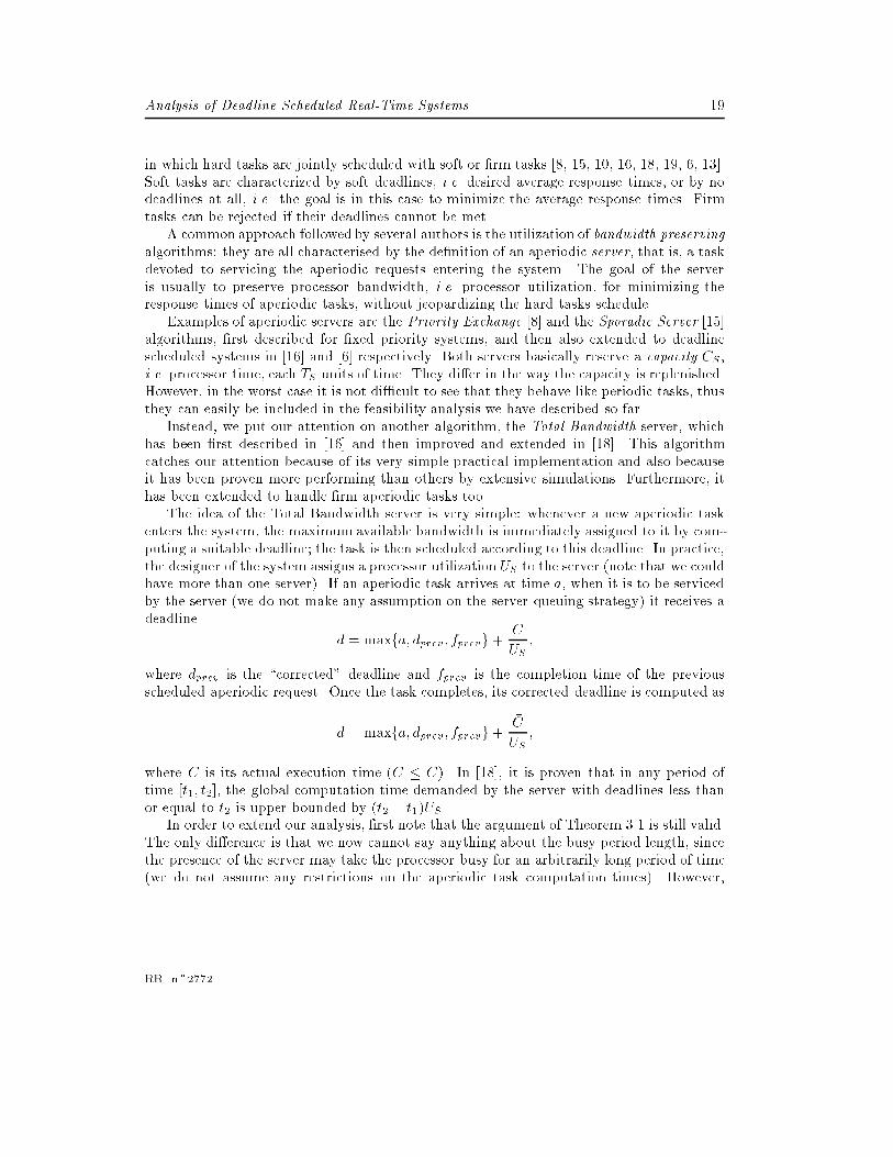
in which hard tasks are jointly scheduled with soft or �rm tasks [8, 15, 10, 16, 18, 19, 6, 13].Soft tasks are characterized by soft deadlines, i.e. desired average response times, or by nodeadlines at all, i.e. the goal is in this case to minimize the average response times. Firmtasks can be rejected if their deadlines cannot be met.
A common approach followed by several authors is the utilization of bandwidth preservingalgorithms: they are all characterised by the de�nition of an aperiodic server, that is, a taskdevoted to servicing the aperiodic requests entering the system. The goal of the serveris usually to preserve processor bandwidth, i.e. processor utilization, for minimizing theresponse times of aperiodic tasks, without jeopardizing the hard tasks schedule.
Examples of aperiodic servers are the Priority Exchange [8] and the Sporadic Server [15]algorithms, �rst described for �xed priority systems, and then also extended to deadlinescheduled systems in [16] and [6] respectively. Both servers basically reserve a capacity CS,i.e. processor time, each TS units of time. They di�er in the way the capacity is replenished.However, in the worst case it is not di�cult to see that they behave like periodic tasks, thusthey can easily be included in the feasibility analysis we have described so far.
Instead, we put our attention on another algorithm, the Total Bandwidth server, whichhas been �rst described in [16] and then improved and extended in [18]. This algorithmcatches our attention because of its very simple practical implementation and also becauseit has been proven more performing than others by extensive simulations. Furthermore, ithas been extended to handle �rm aperiodic tasks too.
The idea of the Total Bandwidth server is very simple: whenever a new aperiodic taskenters the system, the maximum available bandwidth is immediately assigned to it by com-puting a suitable deadline; the task is then scheduled according to this deadline. In practice,the designer of the system assigns a processor utilization US to the server (note that we couldhave more than one server). If an aperiodic task arrives at time a, when it is to be servicedby the server (we do not make any assumption on the server queuing strategy) it receives adeadline
d = maxfa; �dprev; fprevg+C
US;
where �dprev is the \corrected" deadline and fprev is the completion time of the previousscheduled aperiodic request. Once the task completes, its corrected deadline is computed as
�d = maxfa; �dprev; fprevg+�C
US;
where �C is its actual execution time ( �C � C). In [18], it is proven that in any period oftime [t1; t2], the global computation time demanded by the server with deadlines less thanor equal to t2 is upper bounded by (t2 � t1)US .
In order to extend our analysis, �rst note that the argument of Theorem 3.1 is still valid.The only di�erence is that we now cannot say anything about the busy period length, sincethe presence of the server may take the processor busy for an arbitrarily long period of time(we do not assume any restrictions on the aperiodic task computation times). However,
RR n�2772
20 Marco Spuri
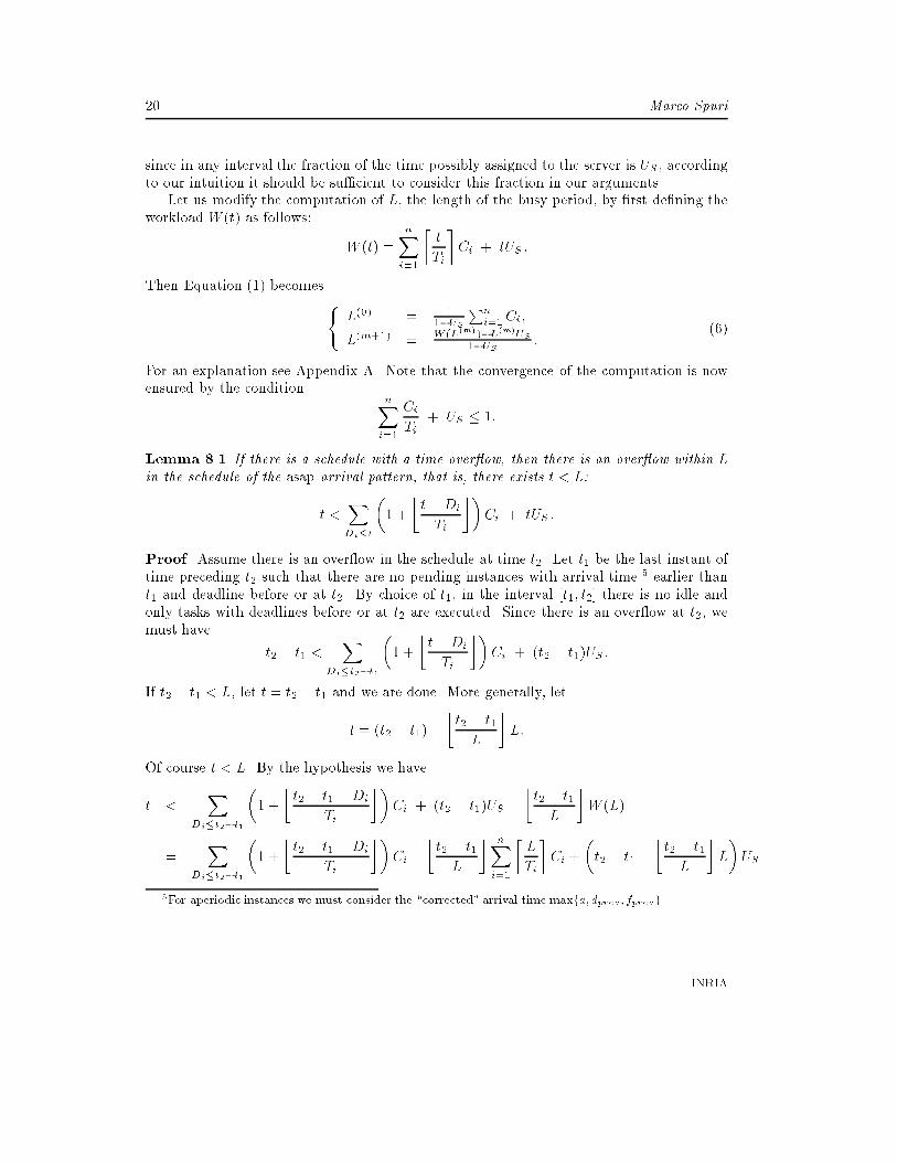
since in any interval the fraction of the time possibly assigned to the server is US , accordingto our intuition it should be su�cient to consider this fraction in our arguments.
Let us modify the computation of L, the length of the busy period, by �rst de�ning theworkload W (t) as follows:
W (t) =nXi=1
�t
Ti
�Ci + tUS :
Then Equation (1) becomes (L(0) = 1
1�US
Pn
i=1Ci;
L(m+1) = W (L(m))�L(m)US1�US
:(6)
For an explanation see Appendix A. Note that the convergence of the computation is nowensured by the condition
nXi=1
Ci
Ti+ US � 1:
Lemma 8.1 If there is a schedule with a time over ow, then there is an over ow within L
in the schedule of the asap arrival pattern, that is, there exists t < L:
t <XDi�t
�1 +
�t �Di
Ti
��Ci + tUS :
Proof. Assume there is an over ow in the schedule at time t2. Let t1 be the last instant oftime preceding t2 such that there are no pending instances with arrival time 5 earlier thant1 and deadline before or at t2. By choice of t1, in the interval [t1; t2] there is no idle andonly tasks with deadlines before or at t2 are executed. Since there is an over ow at t2, wemust have
t2 � t1 <X
Di�t2�t1
�1 +
�t�Di
Ti
��Ci + (t2 � t1)US :
If t2 � t1 < L, let t = t2 � t1 and we are done. More generally, let
t = (t2 � t1) �
�t2 � t1
L
�L:
Of course t < L. By the hypothesis we have
t <X
Di�t2�t1
�1 +
�t2 � t1 �Di
Ti
��Ci + (t2 � t1)US �
�t2 � t1
L
�W (L)
=X
Di�t2�t1
�1 +
�t2 � t1 �Di
Ti
��Ci �
�t2 � t1
L
� nXi=1
�L
Ti
�Ci +
�t2 � t1 �
�t2 � t1
L
�L
�US
5For aperiodic instances we must consider the \corrected" arrival time maxfa; �dprev ; fprevg.
INRIA
Analysis of Deadline Scheduled Real-Time Systems 21
�X
Di�t2�t1
�1 +
�t2 � t1 �Di
Ti
��
�t2 � t1
L
� �L
Ti
��Ci + tUS
�X
Di�t2�t1
1 +
�t2 � t1 �Di
Ti
��
&�t2�t1L
�L
Ti
'!Ci + tUS
�X
Di�t2�t1
1 +
$t2 � t1 �
�t2�t1L
�L �Di
Ti
%!Ci + tUS
=X
Di�t2�t1
�1 +
�t�Di
Ti
��Ci + tUS :
2
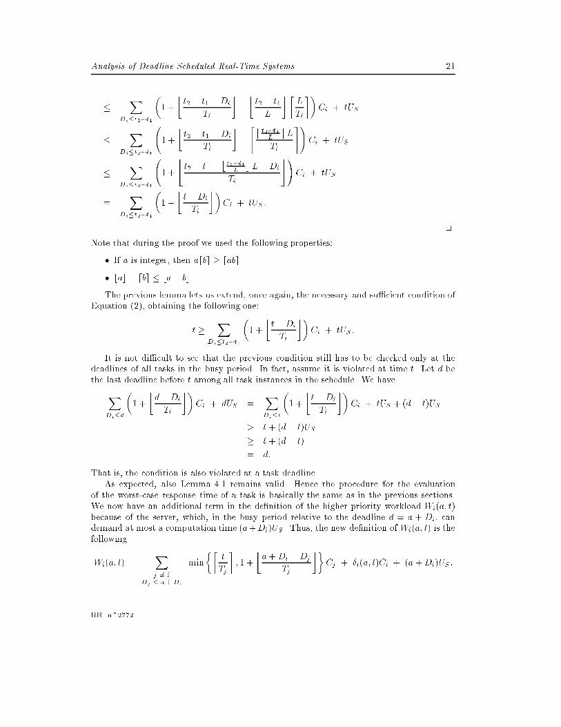
Note that during the proof we used the following properties:
� If a is integer, then adbe � dabe.
� bac � dbe � ba� bc.
The previous lemma lets us extend, once again, the necessary and su�cient condition ofEquation (2), obtaining the following one:
t �X
Di�t2�t1
�1 +
�t�Di
Ti
��Ci + tUS :
It is not di�cult to see that the previous condition still has to be checked only at thedeadlines of all tasks in the busy period. In fact, assume it is violated at time t. Let d bethe last deadline before t among all task instances in the schedule. We have
XDi�d
�1 +
�d�Di
Ti
��Ci + dUS =
XDi�t
�1 +
�t �Di
Ti
��Ci + tUS + (d� t)US
> t + (d� t)US
� t + (d� t)
= d:
That is, the condition is also violated at a task deadline.As expected, also Lemma 4.1 remains valid. Hence the procedure for the evaluation
of the worst-case response time of a task is basically the same as in the previous sections.We now have an additional term in the de�nition of the higher priority workload Wi(a; t)because of the server, which, in the busy period relative to the deadline d = a + Di, candemand at most a computation time (a+Di)US . Thus, the new de�nition of Wi(a; t) is thefollowing
Wi(a; t) =Xj 6= i
Dj � a +Di
min
��t
Tj
�; 1 +
�a+Di �Dj
Tj
��Cj + �i(a; t)Ci + (a +Di)US :
RR n�2772
22 Marco Spuri
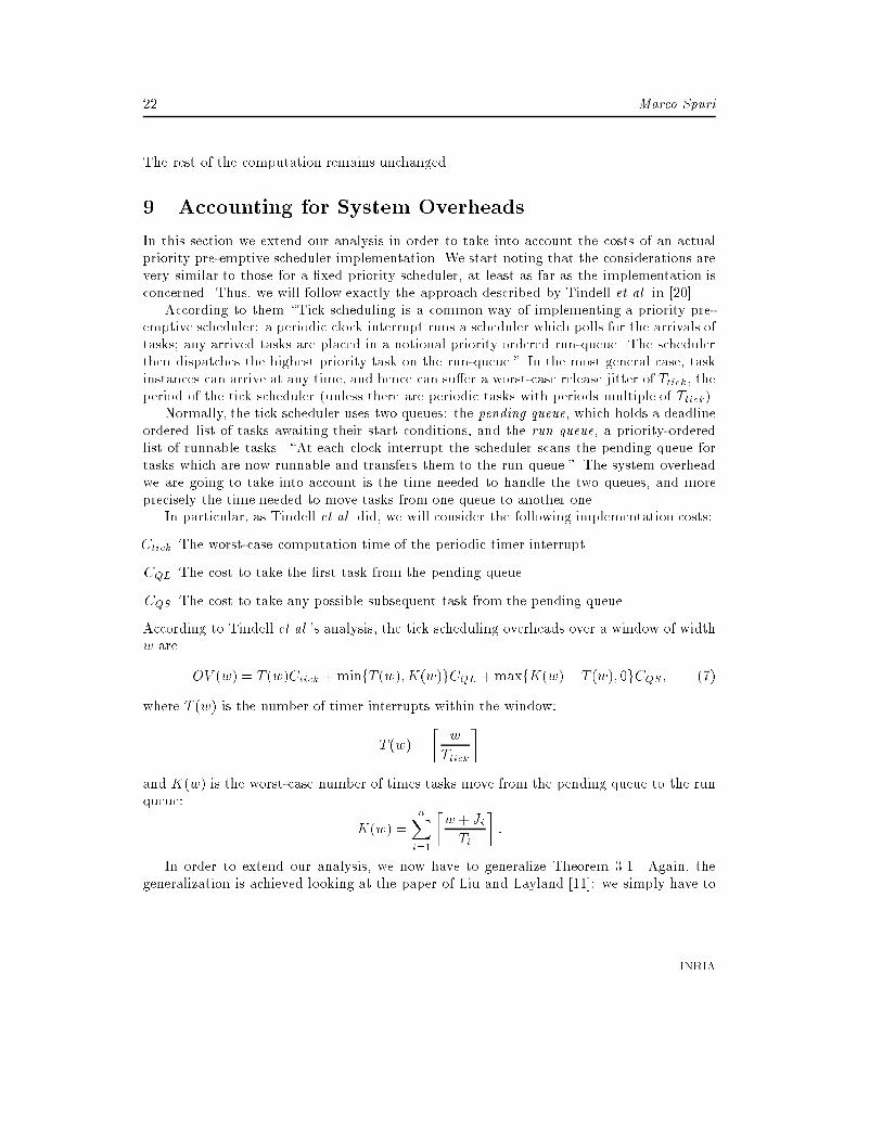
The rest of the computation remains unchanged.
9 Accounting for System Overheads
In this section we extend our analysis in order to take into account the costs of an actualpriority pre-emptive scheduler implementation. We start noting that the considerations arevery similar to those for a �xed priority scheduler, at least as far as the implementation isconcerned. Thus, we will follow exactly the approach described by Tindell et al. in [20].
According to them \Tick scheduling is a common way of implementing a priority pre-emptive scheduler: a periodic clock interrupt runs a scheduler which polls for the arrivals oftasks; any arrived tasks are placed in a notional priority ordered run-queue. The schedulerthen dispatches the highest priority task on the run-queue." In the most general case, taskinstances can arrive at any time, and hence can su�er a worst-case release jitter of Ttick, theperiod of the tick scheduler (unless there are periodic tasks with periods multiple of Ttick).
Normally, the tick scheduler uses two queues: the pending queue, which holds a deadlineordered list of tasks awaiting their start conditions, and the run queue, a priority-orderedlist of runnable tasks. \At each clock interrupt the scheduler scans the pending queue fortasks which are now runnable and transfers them to the run queue." The system overheadwe are going to take into account is the time needed to handle the two queues, and moreprecisely the time needed to move tasks from one queue to another one.
In particular, as Tindell et al. did, we will consider the following implementation costs:
Ctick The worst-case computation time of the periodic timer interrupt.
CQL The cost to take the �rst task from the pending queue.
CQS The cost to take any possible subsequent task from the pending queue.
According to Tindell et al.'s analysis, the tick scheduling overheads over a window of widthw are
OV (w) = T (w)Ctick +minfT (w);K(w)gCQL +maxfK(w)� T (w); 0gCQS; (7)
where T (w) is the number of timer interrupts within the window:
T (w) =
�w
Ttick
�
and K(w) is the worst-case number of times tasks move from the pending queue to the runqueue:
K(w) =nXi=1
�w + Ji
Ti
�:
In order to extend our analysis, we now have to generalize Theorem 3.1. Again, thegeneralization is achieved looking at the paper of Liu and Layland [11]: we simply have to
INRIA
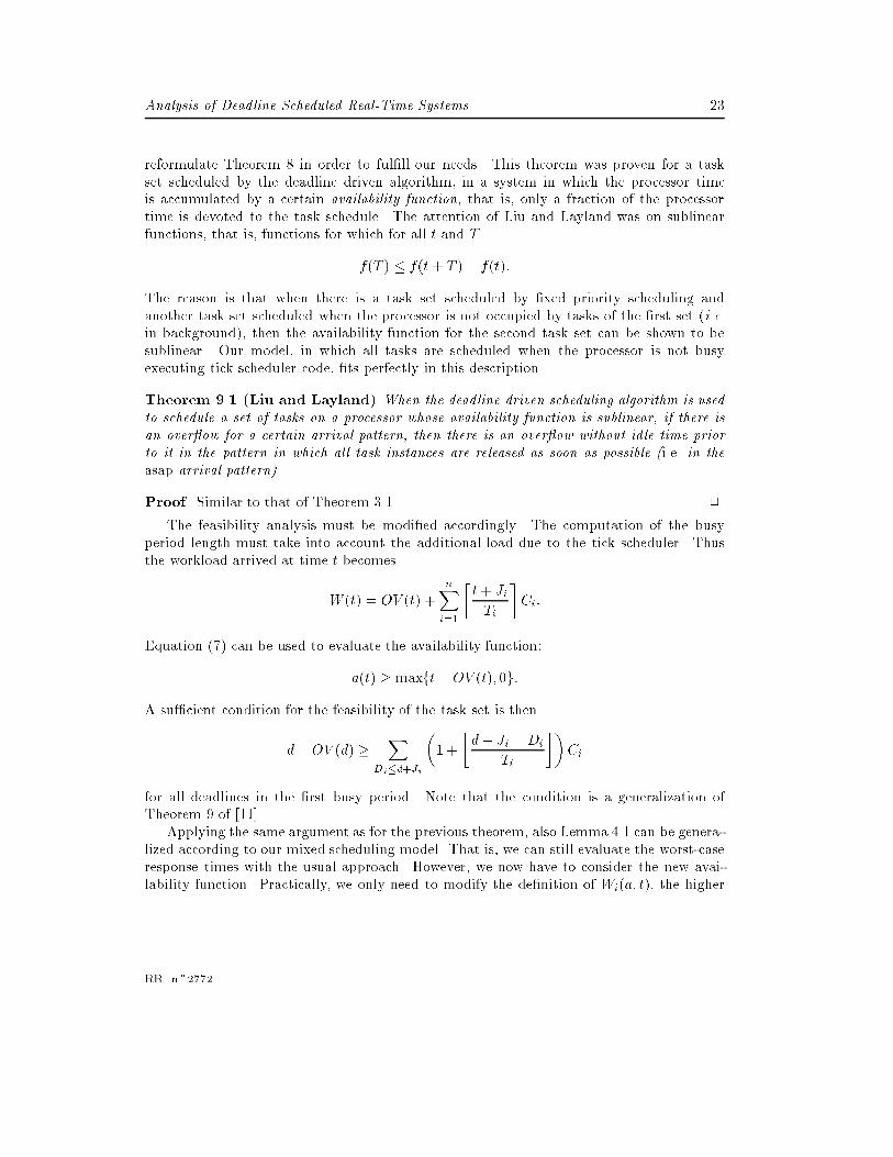
Analysis of Deadline Scheduled Real-Time Systems 23
reformulate Theorem 8 in order to ful�ll our needs. This theorem was proven for a taskset scheduled by the deadline driven algorithm, in a system in which the processor timeis accumulated by a certain availability function, that is, only a fraction of the processortime is devoted to the task schedule. The attention of Liu and Layland was on sublinearfunctions, that is, functions for which for all t and T
f(T ) � f(t + T ) � f(t):
The reason is that when there is a task set scheduled by �xed priority scheduling andanother task set scheduled when the processor is not occupied by tasks of the �rst set (i.e.in background), then the availability function for the second task set can be shown to besublinear. Our model, in which all tasks are scheduled when the processor is not busyexecuting tick scheduler code, �ts perfectly in this description.
Theorem 9.1 (Liu and Layland) When the deadline driven scheduling algorithm is usedto schedule a set of tasks on a processor whose availability function is sublinear, if there isan over ow for a certain arrival pattern, then there is an over ow without idle time priorto it in the pattern in which all task instances are released as soon as possible (i.e. in theasap arrival pattern).
Proof. Similar to that of Theorem 3.1. 2
The feasibility analysis must be modi�ed accordingly. The computation of the busyperiod length must take into account the additional load due to the tick scheduler. Thusthe workload arrived at time t becomes
W (t) = OV (t) +nXi=1
�t+ Ji
Ti
�Ci:
Equation (7) can be used to evaluate the availability function:
a(t) � maxft� OV (t); 0g:
A su�cient condition for the feasibility of the task set is then
d�OV (d) �X
Di�d+Ji
�1 +
�d+ Ji �Di
Ti
��Ci
for all deadlines in the �rst busy period. Note that the condition is a generalization ofTheorem 9 of [11].
Applying the same argument as for the previous theorem, also Lemma 4.1 can be genera-lized according to our mixed scheduling model. That is, we can still evaluate the worst-caseresponse times with the usual approach. However, we now have to consider the new avai-lability function. Practically, we only need to modify the de�nition of Wi(a; t), the higher
RR n�2772
24 Marco Spuri
Semaphore Locked by Time held
1 Task 9 9002 Task 9 3002 Task 15 13503 Task 6 4003 Task 10 4004 Task 3 1004 Task 9 3005 Task 11 7505 Task 15 750
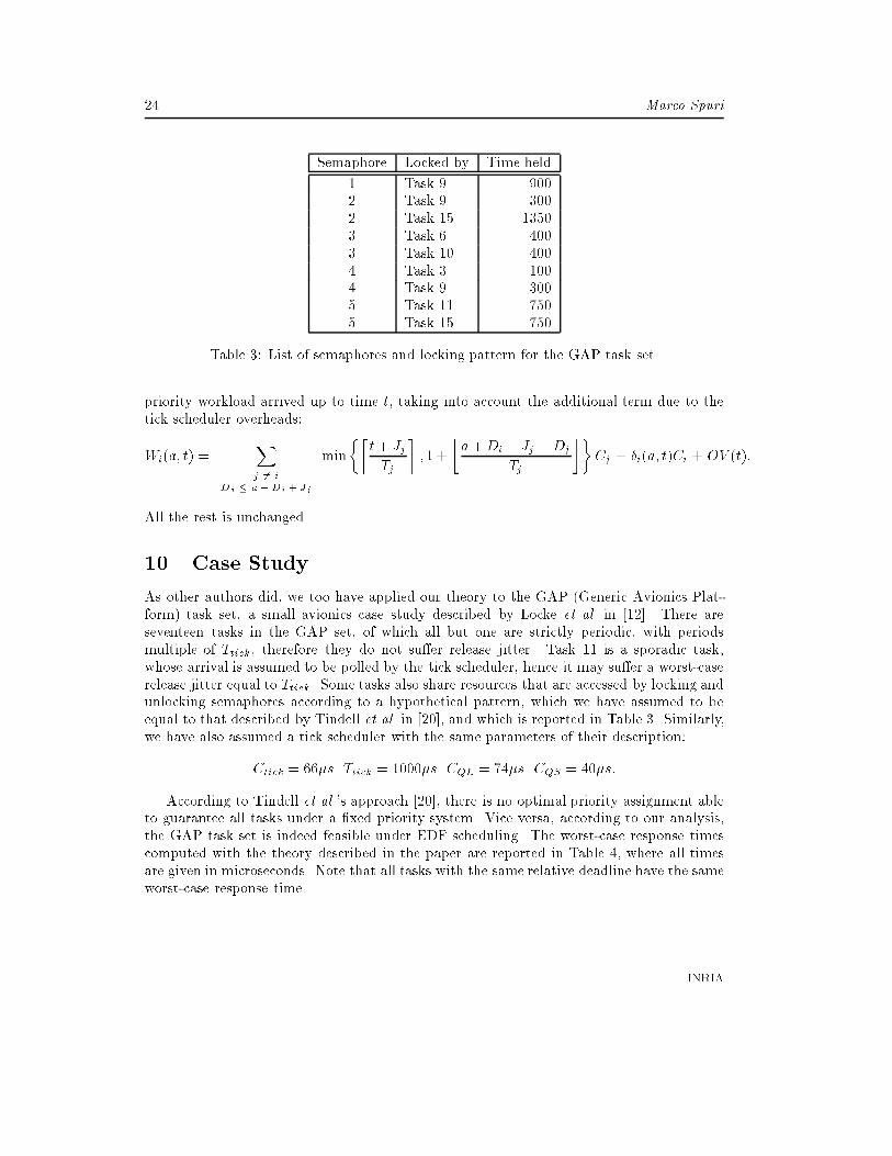
Table 3: List of semaphores and locking pattern for the GAP task set.
priority workload arrived up to time t, taking into account the additional term due to thetick scheduler overheads:
Wi(a; t) =Xj 6= i
Dj � a+Di + Jj
min
��t+ Jj
Tj
�; 1 +
�a+Di + Jj �Dj
Tj
��Cj + �i(a; t)Ci + OV (t):
All the rest is unchanged.
10 Case Study
As other authors did, we too have applied our theory to the GAP (Generic Avionics Plat-form) task set, a small avionics case study described by Locke et al. in [12]. There areseventeen tasks in the GAP set, of which all but one are strictly periodic, with periodsmultiple of Ttick, therefore they do not su�er release jitter. Task 11 is a sporadic task,whose arrival is assumed to be polled by the tick scheduler, hence it may su�er a worst-caserelease jitter equal to Ttick. Some tasks also share resources that are accessed by locking andunlocking semaphores according to a hypothetical pattern, which we have assumed to beequal to that described by Tindell et al. in [20], and which is reported in Table 3. Similarly,we have also assumed a tick scheduler with the same parameters of their description:
Ctick = 66�s Ttick = 1000�s CQL = 74�s CQS = 40�s:
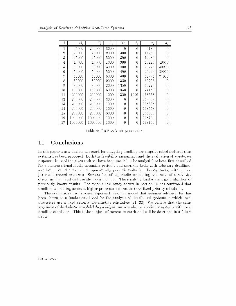
According to Tindell et al.'s approach [20], there is no optimal priority assignment ableto guarantee all tasks under a �xed priority system. Vice versa, according to our analysis,the GAP task set is indeed feasible under EDF scheduling. The worst-case response timescomputed with the theory described in the paper are reported in Table 4, where all timesare given in microseconds. Note that all tasks with the same relative deadline have the sameworst-case response time.
INRIA
Analysis of Deadline Scheduled Real-Time Systems 25
i Di Ti Ci Bi Ji ri ai
1 5000 200000 3000 0 0 4180 02 25000 25000 2000 300 0 12280 03 25000 25000 5000 300 0 12280 04 40000 40000 1000 300 0 20226 400005 50000 50000 3000 400 0 30226 300006 50000 50000 5000 400 0 30226 300007 59000 59000 8000 400 0 39226 210008 80000 80000 9000 1350 0 60226 09 80000 80000 2000 1350 0 60226 010 100000 100000 5000 1350 0 74150 011 200000 200000 1000 1350 1000 168558 012 200000 200000 3000 0 0 168558 013 200000 200000 1000 0 0 168558 014 200000 200000 1000 0 0 168558 015 200000 200000 3000 0 0 168558 016 1000000 1000000 1000 0 0 198760 017 1000000 1000000 1000 0 0 198760 0
Table 4: GAP task set parameters.
11 Conclusions
In this paper a new exible approach for analysing deadline pre-emptive scheduled real-timesystems has been proposed. Both the feasibility assessment and the evaluation of worst-caseresponse times of the given task set have been tackled. The analysis has been �rst describedfor a computational model assuming periodic and sporadic tasks with arbitrary deadlines,and later extended to include sporadically periodic tasks (i.e. bursty tasks) with releasejitter and shared resources. Servers for soft aperiodic scheduling and costs of a real tickdriven implementation have also been included. The resulting analysis is a generalization ofpreviously known results. The avionic case study shown in Section 10 has con�rmed thatdeadline scheduling achieves higher processor utilization than �xed priority scheduling.
The evaluation of worst-case response times, in a model that assumes release jitter, hasbeen shown as a fundamental tool for the analysis of distributed systems in which localprocessors use a �xed priority pre-emptive schedulers [21, 22]. We believe that the sameargument of the holistic schedulability analysis can now also be applied to systems with localdeadline schedulers. This is the subject of current research and will be described in a futurepaper.
RR n�2772
26 Marco Spuri
References
[1] Audsley N., Burns A., Richardson M., Tindell K., and Wellings A.J., \Applying NewScheduling Theory to Static Priority Pre-emptive Scheduling," Software EngineeringJournal, September 1993.
[2] Baker T.P., \Stack-Based Scheduling of Real-time Processes," The Journal of Real-Time Systems 3, pp. 67-99, 1991.
[3] Baruah S.K., Rosier L.E., and Howell R.R., \Algorithms and Complexity Concerningthe Preemptive Scheduling of Periodic, Real-Time Tasks on One Processor," The Jour-nal of Real-Time Systems 2, 1990.
[4] Chen M. and Lin K., \Dynamic Priority Ceilings: A Concurrency Control Protocol forReal-Time Systems," The Journal of Real-Time Systems 2, pp. 325-346, 1990.
[5] Dertouzos M.L., \Control Robotics; the Procedural Control of Physical Processes,"Information Processing 74, 1974.
[6] Ghazalie T.M. and Baker T.P., \Aperiodic Servers in a Deadline Scheduling Environ-ment," The Journal of Real-Time Systems 9, pp. 31-67, 1995.
[7] Katcher D.I., Lehoczky J.P., and Strosnider J.K., \Scheduling Models of Dynamic Prio-rity Schedulers," Research Report CMUCDS-93-4, Carnegie Mellon University, Pitts-burgh, April 1993.
[8] Lehoczky J.P., Sha L., and Strosnider J.K., \Enhanced Aperiodic Responsiveness inHard Real-Time Environments," Proc. of the 8th IEEE Real-Time Systems Symposium,December 1987.
[9] Lehoczky J.P., \Fixed Priority Scheduling of Periodic Task Sets with Arbitrary Dead-lines," Proc. of the 11th IEEE Real-Time Systems Symposium, December 1990.
[10] Lehoczky J.P. and Ramos-Thuel S., \An Optimal Algorithm for Scheduling Soft-Aperiodic Tasks in Fixed-Priority Preemptive Systems," Proc. of the 13th IEEE Real-Time Systems Symposium, December 1992.
[11] Liu C.L. and Layland J.W., \Scheduling algorithms for multiprogramming in a hardreal-time environment," Journal of ACM 20(1), pp. 40-61, January 1973.
[12] Locke C.D., Vogel D.R., and Mesler T.J., \Building a Predictable Avionics Platform inAda: A Case Study," Proc. of the IEEE Real-Time Systems Symposium, 1991.
[13] Ramamritham K., \Dynamic Priority Scheduling," in Real-Time Systems: Speci�ca-tion, Veri�cation and Analysis, edited by Mathai Joseph, Prentice Hall, November1995.
INRIA
Analysis of Deadline Scheduled Real-Time Systems 27
[14] Sha L., Rajkumar R. and Lehoczky J.P., \Priority Inheritance Protocols: An Approachto Real-Time Synchronization," IEEE Transactions on Computers 39(9), September1990.
[15] Sprunt B., Sha L., and Lehoczky J.P., \Aperiodic Task Scheduling for Hard-Real-TimeSystems," The Journal of Real-Time Systems 1, pp. 27-60, 1989.
[16] Spuri M. and Buttazzo G., \E�cient Aperiodic Service under Earliest Deadline Sche-duling," Proc. of the 15th IEEE Real-Time Systems Symposium, December 1994.
[17] Spuri M., \Earliest Deadline Scheduling in Real-Time Systems," Doctorate dissertation,Scuola Superiore S.Anna, Pisa, 1995.
[18] Spuri M., Buttazzo G., and Sensini F., \Robust Aperiodic Scheduling under DynamicPriority Systems," Proc. of the 16th IEEE Real-Time Systems Symposium, December1995.
[19] Spuri M. and Buttazzo G., \Scheduling Aperiodic Tasks in Dynamic Priority Systems,"The Journal of Real-Time Systems, to appear.
[20] Tindell K., Burns A., and Wellings A.J., \An Extendible Approach for Analysing FixedPriority Hard Real-Time Tasks," The Journal of Real-Time Systems 6(2), 1994.
[21] Tindell K. and Clark J., \Holistic Schedulability Analysis for Distributed Hard Real-Time Systems," Microprocessors and Microprogramming 40, 1994.
[22] Tindell K., Burns A., and Wellings A.J., \Analysis of Hard Real-Time Communica-tions," The Journal of Real-Time Systems 9, 1995.
A Busy Period Properties
A.1 Convergence and Complexity of Iterative Formulae
Both in the feasibility analysis and in the evaluation of worst-case response times describedin the paper, we compute busy period lengths by means of iterative formulae. We previouslystated that the convergence of these formulae in a �nite number of steps is ensured by thecondition
nXi=1
Ci
Ti+ US � 1;
which is our �rst requirement, because if the condition does not hold the task set is surelynot feasible.
We now prove the statement for the computation of the busy period length L in ourmodel of Section 8, namely, Equation (6). First note that the workload function W (t) is a
RR n�2772
28 Marco Spuri
L(4)L(3)L(0) L(1) L(2)
W(t)
tL(5)
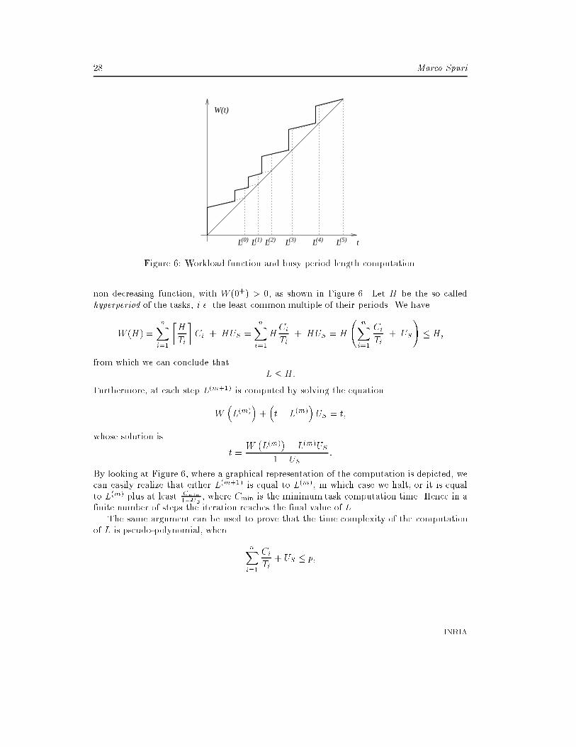
Figure 6: Workload function and busy period length computation.
non decreasing function, with W (0+) > 0, as shown in Figure 6. Let H be the so calledhyperperiod of the tasks, i.e. the least common multiple of their periods. We have
W (H) =nXi=1
�H
Ti
�Ci + HUS =
nXi=1
HCi
Ti+ HUS = H
nXi=1
Ci
Ti+ US
!� H;
from which we can conclude thatL � H:
Furthermore, at each step L(m+1) is computed by solving the equation
W�L(m)
�+�t� L(m)
�US = t;
whose solution is
t =W�L(m)
�� L(m)US
1� US:
By looking at Figure 6, where a graphical representation of the computation is depicted, wecan easily realize that either L(m+1) is equal to L(m), in which case we halt, or it is equalto L(m) plus at least Cmin
1�US, where Cmin is the minimum task computation time. Hence in a
�nite number of steps the iteration reaches the �nal value of L.The same argument can be used to prove that the time complexity of the computation
of L is pseudo-polynomial, when
nXi=1
Ci
Ti+ US � p;
INRIA
Analysis of Deadline Scheduled Real-Time Systems 29
for some constant p < 1. We only need to �nd a tighter upper bound for L:
L =nXi=1
�L
Ti
�Ci + LUS �
nXi=1
�1 +
L
Ti
�Ci + LUS =
nXi=1
Ci + L
nXi=1
Ci
Ti+ US
!;
from which we obtain
L �
Pn
i=1 Ci
1��Pn
i=1CiTi
+ US
� �
Pn
i=1Ci
1� p:
Since each step of the iterative formula takes O(n) time, the whole computation then takesO(n
Pn
i=1Ci) time, which is, as claimed, a psuedo-polynomial complexity. Note that thisalso implies a pseudo-polynomial time complexity for both the procedures of feasibilityassessment and worst-case response times evaluation. Whether a full polynomial time algo-rithm exists for the feasibility assessment problem is still an open question [3].
A.2 Maximum Busy Period Length
Using again the `shift' argument, we can easily prove that the length L of the �rst busyperiod in the schedule of the asap arrival pattern is the maximum length of any possiblebusy period in any schedule. Consider a busy period in the schedule of a given arrivalpattern. Let L0 be its length. The beginning of the period must coincide with the release ofa task instance. If we ideally shift left all other subsequent task instances, so as to obtainan asap arrival pattern starting at the beginning of the busy period, the workload arrivedwithin the period can only increase, i.e. the length of the new busy period cannot be lessthan L0. The busy period obtained in this way is exactly the �rst one in the schedule of theasap arrival pattern, that is, L0 � L.
B Full Analysis Description
In this appendix we fully describe the analysis for a system with the following characteristics:
� the task set is modelled by sporadically periodic arrival laws;
� all tasks can experience release jitter and can share resources by locking semaphores,according to a speci�c concurrency control protocol like the Dynamic Priority Ceilingor the Stack Resource Policy;
� a Total Bandwidth server with processor utilization US is included for handling eithersoft aperiodic tasks or �rm aperiodic tasks (in a more general situation we could havemore than one server, however, the analysis would not di�er signi�cantly);
� a tick scheduler with relative run-time costs is also considered.
RR n�2772
30 Marco Spuri
We also assume thatCtick
Ttick+
nXi=1
Ci
Ti+ US � 1;
which is a necessary condition for the feasibility of the task set. Both the feasibility analysisand the computation of the worst-case response times are summarized.
B.1 Feasibility Analysis
The analysis proceeds in two steps: �rstly we compute the length of the initial busy periodin the schedule of the asap arrival pattern, and then we check all deadlines in the period.The busy period length L is computed by means of the following iterative formula:(
L(0) = 11�US
Pn
i=1Ci;
L(m+1) = W (L(m))�L(m)US1�US
;
where W (t) is the cumulative workload arrived before time t:
W (t) = OV (t) +nXi=1
Ii(t)Ci + tUS :
Ii(t) is the number of instances of task i arrived and released by time t:
Ii(t) =
�t+ Ji
Ti
�ni +min
8<:ni;
2666t+ Ji �
jt+JiTi
kTi
ti
37779=; :
OV (t) is the overhead of the tick scheduler:
OV (t) = T (t)Ctick +minfT (t);K(t)gCQL +maxfK(t)� T (t); 0gCQS;
where T (t) is the number of timer interrupts within time t:
T (t) =
�t
Ttick
�
and K(t) is the worst-case number of times tasks move from the pending queue to the runqueue:
K(t) =nXi=1
Ii(t):
Once determined L, the feasibility of the task set is established by checking for anydeadline d � L in the asap arrival pattern the following condition:
d� OV (d) �X
Di�d+Ji
Hi(d)Ci + dUS + Bk(d);
INRIA
Analysis of Deadline Scheduled Real-Time Systems 31
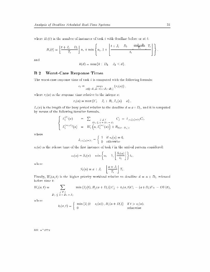
where Hi(t) is the number of instances of task i with deadline before or at t:
Hi(t) =
�t+ Ji �Di
Ti
�ni +min
8<:ni; 1 +
6664 t+ Ji �Di �jt+Ji�Di
Ti
kTi
ti
77759=; ;
andk(d) = maxfk : Dk � Jk � dg:
B.2 Worst-Case Response Times
The worst-case response time of task i is computed with the following formula:
ri = maxa2[�Ji;L�Ci�Ji�Bi)
fri(a)g ;
where ri(a) is the response time relative to the integer a:
ri(a) = maxfCi + Ji + Bi; Li(a) � ag :
Li(a) is the length of the busy period relative to the deadline d = a+Di, and it is computedby means of the following iterative formula:8><
>:L(0)i (a) =
Pj 6= i
Dj � a+Di + Jj
Cj + Ifsi(a)=0gCi;
L(m+1)i (a) = Wi
�a; L
(m)i (a)
�+Bk(a+Di);
where
Ifsi(a)=0g =
�1 if si(a) = 0,0 otherwise.
si(a) is the release time of the �rst instance of task i in the arrival pattern considered:
si(a) = Si(a)�min
�ni � 1;
�Si(a)
ti
��ti;
where
Si(a) = a+ Ji �
�a+ Ji
Ti
�Ti:
Finally, Wi(a; t) is the higher priority workload relative to deadline d = a + Di, releasedbefore time t:
Wi(a; t) =Xj 6= i
Dj � a+Di + Jj
minfIj(t);Hj(a+Di)gCj + �i(a; t)Ci + (a+Di)US + OV (t);
where
�i(a; t) =
�minfIi (t� si(a)) ;Hi(a+Di)g if t > si(a),0 otherwise.
RR n�2772
Unité de recherche INRIA Lorraine, Technopôle de Nancy-Brabois, Campus scientifique,615 rue du Jardin Botanique, BP 101, 54600 VILLERS LÈS NANCY
Unité de recherche INRIA Rennes, Irisa, Campus universitaire de Beaulieu, 35042 RENNES CedexUnité de recherche INRIA Rhône-Alpes, 46 avenue Félix Viallet, 38031 GRENOBLE Cedex 1
Unité de recherche INRIA Rocquencourt, Domaine de Voluceau, Rocquencourt, BP 105, 78153 LE CHESNAY CedexUnité de recherche INRIA Sophia-Antipolis, 2004 route des Lucioles, BP 93, 06902 SOPHIA-ANTIPOLIS Cedex
ÉditeurINRIA, Domaine de Voluceau, Rocquencourt, BP105, 78153 LE CHESNAY Cedex (France)
ISSN 0249-6399