Introduction to SPSS

1.Introduction………………………………………………………….31.1SPSS Data files

2. Coding and Entering Data…………………………………………42.1 Coding Data (Variable View)2.2 Entering Data (Data View)

3.Descriptive Statistics………………………………………………..93.1 Frequency Distribution3.2 Crosstabs3.3 Correlation3.4 Means

4. Independent Sample T-test ………………………………………16

2

1. INTRODUCTIONStatistical Package for the Social Sciences (SPSS) is a very powerful Data Analysis Application. It provides a user-friendly tool for analysing Questionnaire Data and other Data Sets. It can also be used in conjunction with most standard spreadsheet and word processing packages to produce professional reports on the findings of any Analysis.

1.1 SPSS DATA FILESOnce SPSS is activated the user is presented with the SPSS Screen. A new Data file is opened automatically. This file contains two Windows, a Data View and a Variable View

(i) Data View

This Data View consists of a grid of Columns and Rows, similar to a spreadsheet. The Columns represent Variables and the Rows represent Cases. The numerical data from the questionnaire are typed in this Window

(ii) Variable View

The variable view also contains a grid of rows and columns. In this Window the rows represent the variables in the analysis and the columns are used to define the characteristics of each variable. We will discuss this in greater detail in the next section.

3

2. CODING AND ENTERING DATA

2.1 Coding DataWhen processing data it is essential to develop a coding system. This is a system of numerical codes representing different values in the data set. In SPSS the user can enter this coding system using the Variable View Window. To illustrate this process we will look at a simple questionnaire and show how this should be coded in SPSS. This questionnaire is shown is Appendix A.

The first Question is: What is your gender?

and the codes for the responses are 1 = Male and

2 = FemaleHow can we represent this variable in SPSS.

Variable ViewTo code a variable in SPSS we first need to enter the Variable View by clicking the Variable View tab at the bottom of the screen.

Variable NameIn the first column enter the variable name. The variable name can be up to 64 characters in length (no spaces). For the first variable in the questionnaire we can use the name Gender.

Variable TypeThe Variable Type allows the used enter the data in different forms, numerical, string, date etc. In quantitative research projects it is recommended to always use Numeric Type where possible and this is the default in SPSS.

Width and DecimalsWidth and Decimals will be entered automatically and are only used for presentation purposes

Variable Label (Optional)If required enter a Label in the box provided. The Variable Label provides a more detailed description of the question than the Variable Name, as it can contain many more characters. In our example we might enter ‘What is your gender’ as the Variable Label. If this variable is used in any analysis it is the Variable Label that appears in the Output. If no Variable Label is entered then the Variable Name is used in any Output.

4

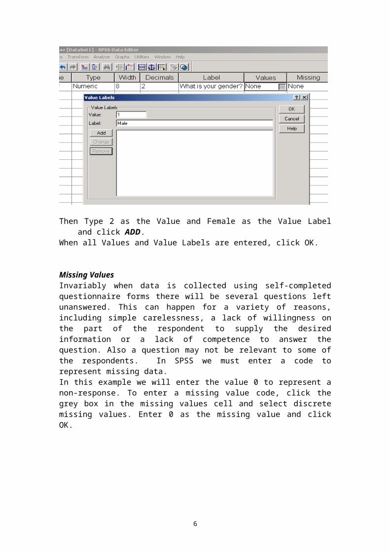
ValuesValue labels are used to define the coding system for the variable. To define a coding system for a variable, click on the Values cell and then click the little grey box in the cell. Type the Value and the corresponding Value Label in the boxes provided. For the gender variable Type 1 as the Value and Male as the Value Label and then click the ADD button.

Then Type 2 as the Value and Female as the Value Label and click ADD. When all Values and Value Labels are entered, click OK.

Missing ValuesInvariably when data is collected using self-completed questionnaire forms there will be several questions left unanswered. This can happen for a variety of reasons, including simple carelessness, a lack of willingness on the part of the respondent to supply the desired information or a lack of competence to answer the question. Also a question may not be relevant to some of the respondents. In SPSS we must enter a code to represent missing data.In this example we will enter the value 0 to represent a non-response. To enter a missing value code, click the grey box in the missing values cell and select discrete missing values. Enter 0 as the missing value and click OK.

5

To practice what we have just learned and to illustrate two other points lets now code some of the other variables on the questionnaire

Q2. What level of education have you achieved?Bachelors 1 Masters 2 PhD 3

Question 2 can be coded using the same steps as Question 1

Q3. What is your age ____Question 3 is relatively easy to code as it does not need value labels, because the responses to the questions are numerical

Q4.Do you find time to relax?Always 1 Usually 2 Sometimes 3 Rarely 4 Never 5Q5.Do you ever feel stressed at work?Always 1 Usually 2 Sometimes 3 Rarely 4 Never 5Questions 4 and 5 can also be coded like question 1. Notice that the responses to both questions are the same. To save time you can copy the labels from Question 4 and paste them in Question 5.

Q6. Does your job involve the following tasksEvaluating Staff ___Managing Staff ___Training Staff ___

Question 6 is a multiple response question. The respondent is being asked three questions, namely:

Does your job involve training staff?Does your job involve managing staff?Does your job involve evaluating staff?

The respondent can tick all three responses or none or any combination of them, so you will need three variables to represent this question.

Call these variables Task1, Task2 and Task3, use the three questions as the Variable labels and use the Values 1=Yes and 2= No for each variable.

Your final variable view should look like this. Don’t worry if you used different Variable names. All questions are now coded in the SPSS File.

6

2.2 Entering DataTo enter data to a SPSS file we must first return to the Data View. Data is simply typed into the appropriate cell with each cell representing one individual’s answer to a given question.

The next screen contains the data for a number of respondents to this questionnaire.

From this data we can see that the first respondent is Male (gender = 1), is aged 55 has a postgraduate degree (Educ=1), usually finds time to relax, is never stressed at work etc.

Now, enter some data into your own file. You can make up your responses.

7

Finally save the data file using the File Menu. The File Menu is SPSS is similar to other standard Windows packages. SPSS data files are given the prefix .sav, for instance we could call this file “data.sav”.

8

3. DESCRIPTIVE STATISTICSDescriptive Statistics are a group of techniques for describing the breakdown of a variable or variables. They include Frequency Tables (simply tables and charts), Crosstabs, Mean Scores, and other Statistics.

To illustrate the use of these techniques we will use the ‘staff data’ file.

3.1 FrequenciesThe Frequencies procedure provides basic statistics, tables and graphical displays that are useful for describing many types of variables. For a first look at your data, the Frequencies procedure is a good place to start.

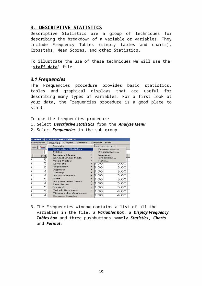
To use the frequencies procedure 1. Select Descriptive Statistics from the Analyse Menu 2. Select Frequencies in the sub-group

3. The Frequencies Window contains a list of all the variables in the file, a Variables box, a Display Frequency Tables box and three pushbuttons namely Statistics, Charts and Format.

9

4. Select the variables you are interested in from the Variables list on the left and place them in the Variables Box on the right (using the arrow in the center). For this exercise, choose “Do you find time to relax” and “Do you ever feel stressed”.

5. For a Frequency Distribution Table tick the Display Frequency Distribution box. (This will be ticked by default)

6. If you require a chart click the Charts Button and choose the type of chart required. There are three basic charts available, Pie Charts, Bar Charts and Histograms. In this case choose a Bar Chart.A selection of basic statistical values like the mean, standard deviation and others are available by clicking the Statistics button. To select the appropriate statistic simply click the adjoining circle (see below). In this case select the mean and the standard deviation.When all required statistics have been chosen click Continue

7. Finally once all Statistics and Charts have been selected click OK

Below we can see some of the SPSS Output from the Frequency Command

Frequency Tables

Do you find time to relax?

Frequency Percent Valid PercentCumulative

PercentValid Always 15 11.0 11.0 11.0

Usually 62 45.6 45.6 56.6

Sometimes 51 37.5 37.5 94.1

Rarely 8 5.9 5.9 100.0

Total 136 100.0 100.0

10

Statistics

Statistics

Do you find

time to relax?

Do you ever feel stressed at

work?N Valid 136 134

Missing 0 2Mean 2.3824 3.4030Std. Deviation .76069 1.03415

Charts

11

3.2 CrosstabsA Crosstab is an extension of a frequency table to 2 or more variables. For example you may wish to look at a breakdown of level of education by gender. To create a Crosstab Table1. Select Descriptive Statistics from the Analyse Menu 2. Select Crosstabs in the sub-group3. From the Variable List select the variable(s) to represent the columns and place in

the Columns box. For this exercise select Gender.4. Do the same thing for the rows box. Select Education Level for the rows.

5. To add percentages click the Cells Button6. Choose the percentage syntax required (e.g. column percentages) by clicking the

appropriate circle.

7. Press Continue8. Finally click OK

The SPSS Output for this Crosstab can be seen on the next page

12

What level of education have you achieved? * What is your gender Crosstabulation

What is your gender

TotalMALE FEMALEWhat level of education have you achieved?

Post Graduate Studies Count 42 14 56

% within What is your gender 40.4% 43.8% 41.2%

Primary Degree Count 56 16 72

% within What is your gender 53.8% 50.0% 52.9%

Leaving Cert Count 6 2 8

% within What is your gender 5.8% 6.3% 5.9%

Total Count 104 32 136% within What is your gender 100.0% 100.0% 100.0%

3.3 Correlation1. Select Correlate from the Analyse Menu 2. Select Bivariate3. From the Variable List select the variables you wish to correlate. Choose Age and

Number of years in the organisation

4. Select the Pearson Correlation Coefficient5. Press Continue

13

The Output for this correlation is shown below:

Correlation Age vs. Tenure

SPSS Output

Correlations

What is your

age

How many

years are you in

the

organisation?

What is your age Pearson Correlation 1 .863**

Sig. (2-tailed) .000

N 136 135

How many years are you in

the organisation?

Pearson Correlation .863** 1

Sig. (2-tailed) .000

N 135 135

**. Correlation is significant at the 0.01 level (2-tailed).

Correlation between age and number of years in organisation is .863. This indicates a positive relationship between the two variables, which is exactly what we would expect.

Note the two asterisks beside the correlation. This indicates that the correlation is statistically significant.

14

3.4 MeansThis functions allows the user calculate the mean score of a dependent variable across the various sub-categories of the independent variable. For example, in our case study we could look at the average age of staff members with different level of education

1. Select Compare Means from the Analyse Menu2. Select Means3. Select the dependent variable(s) from the Variable List. Choose age for this example:4. Select the Independent variable(s) form the Variable List. Choose Level of Education for this example:

5. Click OK

Here is the associated Output from SPSS

Report

What is your age?

What level of education have you achieved? Mean N Std. DeviationPost Graduate Studies 44.1250 56 9.61639Primary Degree 45.9167 72 9.38196Leaving Cert 47.7500 8 4.71320Total 45.2868 136 9.28711

15

4. Independent Sample T-test

To illustrate the use of the independent sample t-test we will use the ‘T-Test’ file.

Independent Sample T-Test2 Independent Groups, 1 Ratio/Interval Test Variable

Part of the turnover intention case study involved examining differences between the two departments in the organisation, for the four key quantitative measures. (Job Satisfaction, Satisfaction with Supervisor, Commitment, Turnover Intention)

As these variables are interval variables and the test is examining the difference between two groups, the independent sample t-test is used.

- In Analyse Menu Click Compare Means- Select Independent Sample T-test

- Select Test Variable(s) from Variable List(Job Satisfaction,Satisfaction with Supervisor,Commitment,Turnover Intention)

- Select Grouping Variable from Variable List (Department)

- Click Define Groups button.

- Insert the value labels representing the two independent groups; enter 1 as Group 1 and 2 as Group 2. (1=Department A, 2=Department B)

- Click Continue- Click OK

16

The SPSS Output from this test, an explanation of this output and how it should be presented are shown on the next page.

SPSS OutputGroup Statistics

Department N Mean Std. DeviationStd. Error

MeanJob Satisfaction A 56 3.7500 .62361 .08333

B 44 4.0455 .60826 .09170Satisfaction with Supervisor

A 56 3.1071 .91666 .12249B

44 3.6369 .76160 .11481

Commitment A 56 2.9420 .58434 .07809B 44 3.4290 .60184 .09073

Turnover Intention A 56 2.6131 1.26775 .16941B 44 2.1061 .89723 .13526

Independent Samples Test

.213 .646 -2.377 98 .019 -.29545

-2.384 93.497 .019 -.29545

.721 .398 -3.086 98 .003 -.52976

-3.155 97.669 .002 -.52976

.713 .401 -4.083 98 .000 -.48701

-4.068 91.181 .000 -.48701

6.719 .011 2.246 98 .027 .50703

2.339 97.036 .021 .50703

Equal variancesassumed

Equal variancesnot assumed

Equal variancesassumed

Equal variancesnot assumed

Equal variancesassumed

Equal variancesnot assumed

Equal variancesassumed

Equal variancesnot assumed

Job Satisfaction

Satisfaction withSupervisor

Commitment

Turnover Intention

F Sig.

Levene's Test forEquality of Variances

t df Sig. (2-tailed)Mean

Difference

t-test for Equality of Means

Interpretation and Presentation

These test results indicate significant differences between the two departments in the organisation. Turnover Intention is significantly higher in Department A (p=.021<0.05). In addition, job satisfaction (p=.019<0.05), commitment to the organisation (p=.000 <0.01) and satisfaction with supervisor (p=.027<0.01) are significantly lower in Department A.

17

These results are commonly presented in the following table format:

Department N Mean S. Dev P-ValueJob Satisfaction A 56 3.75 .62

.019*B 44 4.04 .60

Satisfaction with Supervisor

A 56 3.11 .92.003**

B 44 3.64 .76Commitment

A 56 2.94 .58.000**

B 44 3.43 .60Turnover Intention A 56 2.61 1.26

.021*B 44 2.11 .90

*Significant at the 0.05 level ** Significant at the 0.01 level

APPENDIX A

18

Q1. What is your gender? Male 1 Female 2

Q2. What level of education have you achieved?Bachelors 1 Masters 2 PhD 3

Q3. What is your age ____

Q4. Do you find time to relax?

Always (1) Usually (2) Sometimes (3) Rarely (4) Never (5)

Q5. Do you ever feel stressed at work?

Always (1) Usually (2) Sometimes (3) Rarely (4) Never (5)

Q6. Does your job involve the following tasksEvaluating Staff ___Managing Staff ___Training Staff ___

19