Embed Size (px)
Citation preview


Springer Series on Epidemiology and Health
Series EditorsWolfgang AhrensIris Pigeot
For further volumes:http://www.springer.com/series/7251


Jørn Olsen · Kaare Christensen · Jeff Murray ·Anders Ekbom
An Introduction toEpidemiology for HealthProfessionals
13

Jørn OlsenSchool of Public HealthUniversity of California, Los AngelesLos Angeles CA 90095-1772Box [email protected]
Jeff Murray, MDDepartment of Pediatrics2182 MedLabsUniversity of IowaIowa City, IA [email protected]
Kaare ChristensenInstitute of Public HealthUniversity of Southern DenmarkSdr. Boulevard 23 A5000 Odense [email protected]
Anders EkbomDepartment of Medicine,
Karolinska InstituteSE-171 76 [email protected]
ISSN 1869-7933 e-ISSN 1869-7941ISBN 978-1-4419-1496-5 e-ISBN 978-1-4419-1497-2DOI 10.1007/978-1-4419-1497-2Springer New York Dordrecht Heidelberg London
Library of Congress Control Number: 2010922282
© Springer Science+Business Media, LLC 2010All rights reserved. This work may not be translated or copied in whole or in part without the writtenpermission of the publisher (Springer Science+Business Media, LLC, 233 Spring Street, New York,NY 10013, USA), except for brief excerpts in connection with reviews or scholarly analysis. Use inconnection with any form of information storage and retrieval, electronic adaptation, computer software,or by similar or dissimilar methodology now known or hereafter developed is forbidden.The use in this publication of trade names, trademarks, service marks, and similar terms, even if they arenot identified as such, is not to be taken as an expression of opinion as to whether or not they are subjectto proprietary rights.While the advice and information in this book are believed to be true and accurate at the date of goingto press, neither the authors nor the editors nor the publisher can accept any legal responsibility for anyerrors or omissions that may be made. The publisher makes no warranty, express or implied, with respectto the material contained herein.
Printed on acid-free paper
Springer is part of Springer Science+Business Media (www.springer.com)

Preface
There are many good epidemiology textbooks on the market, but most of these areaddressed to students of public health or people who do clinical research with epi-demiologic methods. There is a need for a short introduction on how epidemiologicmethods are used in public health, genetic and clinical epidemiology, because healthprofessionals need to know basic epidemiologic methods covering etiologic as wellas prognostic factors of diseases. They need to know more about methodology thanintroductory texts on public health have to offer.
In some health faculties, epidemiology is not even part of the teaching curricu-lum. We believe this to be a serious mistake. Medical students are students of allaspects of diseases and health. Without knowing something about epidemiology theclinicians and other health professionals cannot read a growing part of the scien-tific literature in any reasonably critical way and cannot navigate in the world of“evidence-based medicine and evidence-based prevention.” Without skills in epi-demiologic methodology they are in the hands of experts that may not only have aninterest in health.
Some health professionals may believe that only common sense is needed toconduct epidemiological studies, but the scientific literature and the public debateon health issues indicate that common sense is often in short supply and may notthrive without some formal training.
Epidemiologic methods play a key role in identifying environmental, social,and genetic determinants of diseases. Clinical epidemiology addresses the tran-sition from disease to health or toward mortality or social or medical handicaps.Public health epidemiology addresses the transition from being healthy to being nothealthy. Descriptive epidemiology provides the disease pattern that is needed to lookat health in a broad perspective and to set the priorities right. Epidemiology is a basicscience of medicine which addresses key questions such as “Who becomes ill?” and“What are important prognostic factors?” Answers to such questions provide thebasis for better prevention and treatment of diseases.
Many people contributed to the writing of this book: medical students inDenmark, students of epidemiology at the IEA EEPE summer course in Florence,Italy, and students of public health in Los Angeles. Without technical assistance
v

vi Preface
from Gitte Nielsen, Jenade Shelley, Nina Hohe and Pam Masangkay the book wouldnever have materialized.
Los Angeles, California Jørn OlsenOdense, Denmark Kaare ChristensenIowa City, Iowa Jeff MurrayStockholm, Sweden Anders Ekbom
Contents
Part I Descriptive Epidemiology
1 Measures of Disease Occurrence . . . . . . . . . . . . . . . . . . . 3Incidence and Prevalence . . . . . . . . . . . . . . . . . . . . . . . . 4Incidence . . . . . . . . . . . . . . . . . . . . . . . . . . . . . . . . . 6Rates and Dynamic Populations . . . . . . . . . . . . . . . . . . . . . 7Calculating Observation Time . . . . . . . . . . . . . . . . . . . . . . 9Prevalence, Incidence, Duration . . . . . . . . . . . . . . . . . . . . . 10Mortality and Life Expectancy . . . . . . . . . . . . . . . . . . . . . 11Life Expectancy . . . . . . . . . . . . . . . . . . . . . . . . . . . . . 12References . . . . . . . . . . . . . . . . . . . . . . . . . . . . . . . . 13
2 Estimates of Associations . . . . . . . . . . . . . . . . . . . . . . . 15
3 Age Standardization . . . . . . . . . . . . . . . . . . . . . . . . . . 19
4 Causes of Diseases . . . . . . . . . . . . . . . . . . . . . . . . . . . 23References . . . . . . . . . . . . . . . . . . . . . . . . . . . . . . . . 28
5 Descriptive Epidemiology in Public Health . . . . . . . . . . . . . . 29Graphical Models of Causal Links . . . . . . . . . . . . . . . . . . . 33References . . . . . . . . . . . . . . . . . . . . . . . . . . . . . . . . 35
6 Descriptive Epidemiology in Genetic Epidemiology . . . . . . . . . 37Occurrence Data in Genetic Epidemiology . . . . . . . . . . . . . . . 37Clustering of Traits and Diseases in Families . . . . . . . . . . . . . . 38The Occurrence of Genetic Diseases . . . . . . . . . . . . . . . . . . 40References . . . . . . . . . . . . . . . . . . . . . . . . . . . . . . . . 41
7 Descriptive Epidemiology in Clinical Epidemiology . . . . . . . . . 43Sudden Infant Death Syndrome (SIDS) . . . . . . . . . . . . . . . . . 44Cytological Screening for Cervix Cancer . . . . . . . . . . . . . . . . 45Changes in Treatment of Juvenile Diabetes . . . . . . . . . . . . . . . 46References . . . . . . . . . . . . . . . . . . . . . . . . . . . . . . . . 47
vii

viii Contents
Part II Analytical Epidemiology
8 Design Options . . . . . . . . . . . . . . . . . . . . . . . . . . . . . 51Common Designs Used to Estimate Associations . . . . . . . . . . . . 51
Ecological Study . . . . . . . . . . . . . . . . . . . . . . . . . . . 52Case–Control Study . . . . . . . . . . . . . . . . . . . . . . . . . . 54Cohort Study . . . . . . . . . . . . . . . . . . . . . . . . . . . . . 55Experimental Study . . . . . . . . . . . . . . . . . . . . . . . . . . 56
Reference . . . . . . . . . . . . . . . . . . . . . . . . . . . . . . . . 57
9 Follow-Up Studies . . . . . . . . . . . . . . . . . . . . . . . . . . . 59The Non-experimental Follow-Up (Cohort) Study . . . . . . . . . . . 59Studying Risk as a Function of BMI . . . . . . . . . . . . . . . . . . 60Longitudinal Exposure Data . . . . . . . . . . . . . . . . . . . . . . . 62Different Types of Cohort or Follow-Up Studies . . . . . . . . . . . . 63
10 Case–Control Studies . . . . . . . . . . . . . . . . . . . . . . . . . . 67Case–Cohort Sampling . . . . . . . . . . . . . . . . . . . . . . . . . 69Density Sampling of Controls . . . . . . . . . . . . . . . . . . . . . . 69Case–Non-case Study . . . . . . . . . . . . . . . . . . . . . . . . . . 71Patient Controls . . . . . . . . . . . . . . . . . . . . . . . . . . . . . 72Secondary Identification of the Source Population . . . . . . . . . . . 74Case–Control Studies Using Prevalent Cases . . . . . . . . . . . . . . 74When to Do a Case–Control Study? . . . . . . . . . . . . . . . . . . . 77References . . . . . . . . . . . . . . . . . . . . . . . . . . . . . . . . 78
11 The Cross-Sectional Study . . . . . . . . . . . . . . . . . . . . . . . 79
12 The Randomized Controlled Trial (RCT) . . . . . . . . . . . . . . 81Reference . . . . . . . . . . . . . . . . . . . . . . . . . . . . . . . . 84
13 Analytical Epidemiology in Public Health . . . . . . . . . . . . . . 85The Case-Crossover Study . . . . . . . . . . . . . . . . . . . . . . . . 86References . . . . . . . . . . . . . . . . . . . . . . . . . . . . . . . . 87
14 Analytical Epidemiology in Genetic Epidemiology . . . . . . . . . 89Disentangling the Basis for Clustering in Families . . . . . . . . . . . 89
Adoption Studies . . . . . . . . . . . . . . . . . . . . . . . . . . . 89Twin Studies . . . . . . . . . . . . . . . . . . . . . . . . . . . . . . 90Half-Sib Studies . . . . . . . . . . . . . . . . . . . . . . . . . . . . 90
Interpretation of Heritability . . . . . . . . . . . . . . . . . . . . . . . 91Exposure–Disease Associations Through Studies of Relatives . . . . . 91Gene–Environment Interaction . . . . . . . . . . . . . . . . . . . . . 92Cross-Sectional Studies of Genetic Polymorphisms . . . . . . . . . . . 93Incorporation of Genetic Variables in Epidemiologic Studies . . . . . . 93References . . . . . . . . . . . . . . . . . . . . . . . . . . . . . . . . 94

Contents ix
15 Analytical Epidemiology in Clinical Epidemiology . . . . . . . . . 95Common Designs Used to Estimate Associations . . . . . . . . . . . . 95Case-Reports and Cross-Sectional Studies . . . . . . . . . . . . . . . 95Case–Control Studies . . . . . . . . . . . . . . . . . . . . . . . . . . 96Cohort Studies . . . . . . . . . . . . . . . . . . . . . . . . . . . . . . 97Randomized Clinical Trials (RCTs) . . . . . . . . . . . . . . . . . . . 98References . . . . . . . . . . . . . . . . . . . . . . . . . . . . . . . . 99
Part III Sources of Error
16 Confounding and Bias . . . . . . . . . . . . . . . . . . . . . . . . . 103Reference . . . . . . . . . . . . . . . . . . . . . . . . . . . . . . . . 105
17 Confounding . . . . . . . . . . . . . . . . . . . . . . . . . . . . . . 107References . . . . . . . . . . . . . . . . . . . . . . . . . . . . . . . . 111
18 Information Bias . . . . . . . . . . . . . . . . . . . . . . . . . . . . 113References . . . . . . . . . . . . . . . . . . . . . . . . . . . . . . . . 117
19 Selection Bias . . . . . . . . . . . . . . . . . . . . . . . . . . . . . . 119Reference . . . . . . . . . . . . . . . . . . . . . . . . . . . . . . . . 122
20 Making Inference and Making Decisions . . . . . . . . . . . . . . . 123References . . . . . . . . . . . . . . . . . . . . . . . . . . . . . . . . 127
21 Sources of Error in Public Health Epidemiology . . . . . . . . . . . 129Berkson Bias . . . . . . . . . . . . . . . . . . . . . . . . . . . . . . . 131Mendelian Randomization . . . . . . . . . . . . . . . . . . . . . . . . 132References . . . . . . . . . . . . . . . . . . . . . . . . . . . . . . . . 134
22 Sources of Error in Genetic Epidemiology . . . . . . . . . . . . . . 135Multiple Testing . . . . . . . . . . . . . . . . . . . . . . . . . . . . . 135Population Stratification . . . . . . . . . . . . . . . . . . . . . . . . . 136Laboratory Errors . . . . . . . . . . . . . . . . . . . . . . . . . . . . 136
23 Sources of Error in Clinical Epidemiology . . . . . . . . . . . . . . 139Confounding by Indication . . . . . . . . . . . . . . . . . . . . . . . 139Differential Misclassification of Outcome . . . . . . . . . . . . . . . . 140Differential Misclassification of Exposure . . . . . . . . . . . . . . . 141Selection Bias . . . . . . . . . . . . . . . . . . . . . . . . . . . . . . 142References . . . . . . . . . . . . . . . . . . . . . . . . . . . . . . . . 142
Part IV Statistics in EpidemiologyAdditive Model . . . . . . . . . . . . . . . . . . . . . . . . . . . . . 145Multiplicative Model . . . . . . . . . . . . . . . . . . . . . . . . . . . 146Reference . . . . . . . . . . . . . . . . . . . . . . . . . . . . . . . . 150
24 P Values . . . . . . . . . . . . . . . . . . . . . . . . . . . . . . . . . 151

x Contents
25 Calculating Confidence Intervals . . . . . . . . . . . . . . . . . . . 155
Epilogue . . . . . . . . . . . . . . . . . . . . . . . . . . . . . . . . . . . 157Reference . . . . . . . . . . . . . . . . . . . . . . . . . . . . . . . . 157
Index . . . . . . . . . . . . . . . . . . . . . . . . . . . . . . . . . . . . . 159

A Short Introduction to Epidemiology
Epidemiology is an old scientific discipline that dates back to the middle of thenineteenth century. It is a discipline that aims at identifying the determinants ofdiseases and health in populations. It uses a population approach like demogra-phy, perhaps the scientific discipline that most closely resembles epidemiology.Epidemiology is defined by the object of research, “to identity determinants thatchange the occurrence of health phenomena in human populations.”
Epidemiology is often associated with infectious diseases because an epidemicof a disease originally referred to an unexpected rise in the incidence of infectiousdiseases. Epidemiologic methods were first used to study diseases like cholera andmeasles. Now all diseases or health events are studied by means of epidemiologicmethods and these methods are constantly changing to meet these new needs. Eventhe term “epidemic” is used to describe an unexpected increase in the frequency ofany disease such as myocardial infarction, obesity, or asthma.
Today the discipline is used to study genetic, behavioral, and environmentalcauses of infectious and non-infectious diseases. The discipline is used to evalu-ate the effect of treatments or screening and it is the key discipline in the movementthat may have been oversold with the title “evidence-based medicine.”
Public health epidemiology uses the “healthy” population to study the transitionfrom being healthy to being diseased or ill. Clinical epidemiology uses the popu-lation of patients to study predictors of cure or changes in the disease state. Bothdisciplines use experimental and non-experimental methods. Experimental methodsare, however, often not applicable for ethical reasons in public health research sincewe cannot induce possibly harmful exposures on healthy people to address scientifichypotheses.
Epidemiologists have often been actors in political conflicts. Poverty, socialinequalities, unemployment, and crowding are among the main determinants ofhealth [1], and studying these determinants may bring epidemiologists into con-flict with those who benefit from maintaining an unjust society. To some extent,these internal conflicts gave rise to clinical epidemiology. Many clinicians saw aneed for using the methods developed in public health but did not like the idea ofbeing associated with left-wing doctors fighting tuberculosis in India or poverty inLos Angeles. A clinical epidemiologist can study how best to treat diseases withouttaking an interest in how these diseases emerged.
xi

xii A Short Introduction to Epidemiology
We believe time has come to put an end to the artificial separation.Epidemiologists use the same set of tools and the same set of concepts whether theystudy the etiology or the prognosis of disease, although the methodological prob-lems may reflect different circumstances. It is important to give priority to studyingcausal mechanisms that are amenable to intervention whether they affect preventionor treatment.
Epidemiology is among the basic medical sciences but is not quite recognized assuch in many countries. Preventive medicine has been neglected by “patient-directedmedicine” and been referred to specialists outside the clinical world. The process ofevaluating new drugs has been left almost entirely to the pharmaceutical industry,not only to sponsor these studies but also to conduct and analyze the results.
Health professionals have to decide on treatments, perform diagnostic proce-dures, and give advice on prevention. This cannot be done without keeping an eyeon the scientific literature, and at present a large part of what is published in medi-cal journals is based on epidemiologic research. The same is true for much of theinformation that comes from pharmaceutical industries. Without some basic under-standing of the limitations and sources of bias in this literature the clinician becomesa prisoner of his/her own ignorance; an easy victim of incorrect interpretations ofdata. Epidemiology may be the water that is needed in this desert of seduction.
Our intention has been to distill what is needed in the ordinary curriculum forhealth professionals who received an education without being exposed to epidemi-ologic textbooks. We present first a short introduction to the most common typesof epidemiologic studies, how they are used, and their limitations. We then pro-vide examples of how these methods have been used in public health, geneticepidemiology, and clinical research. Although each of these sub-disciplines has itsown set of methods, most studies rely on the same basic set of logical reasoning.We leave out the statistical part of analyzing data and refer readers who take aninterest in this to the many textbooks on this topic. We also refer readers to othertextbooks to study the history of epidemiology [2]. Doing epidemiologic researchrequires following ethical standards and good practice rules for securing confidentialdata. We recommend reading the IEA guidelines on Good Epidemiologic Practice(www.ieaweb.org).
The book is short and condensed, but people in medical professions are cleverand are trained in absorbing abstract information rapidly. Epidemiology is trainingin logical thinking rather than in memorization and we hope this book will be apleasant journey into a mindset for later expansion and use. Keep in mind that animportant part of learning is also to be able to identify what you do not know butshould be aware of before you express your opinion.
References
1. Frank JP. Academic address on the people’s misery: mother of all diseases. Bull Hist Med 1941[first published 1790];9:88–100.
2. Holland WW, Olsen J, Florey CDV (eds.). Development of Epidemiology: Personal Reportsfrom Those Who Were There. Oxford University Press, Oxford, 2007.

Part IDescriptive Epidemiology

Chapter 1Measures of Disease Occurrence
Setting priorities in public health planning for disease prevention depends on a set ofconditions. Public health priorities should be set by the combination of how seriousdiseases are (a product of their frequency and the impact they have on those affectedand society) and our ability to change their frequency or severity. This interventionrequires knowledge of how to treat and/or to prevent the disease. If we have suffi-cient knowledge about the causes of the disease and if these causes are avoidable wemay be able to propose effective preventive programs. If we do not have that knowl-edge research is needed, and if we know where to search for causes this researchcan be specifically targeted. If the disease can be treated at a low cost and with littlerisk, prevention need not be better than cure but often will be.
Clinical medicine may have a tendency to focus on rare but interesting diseases,whereas public health should focus on the big picture taking the frequency of diseaseinto consideration. What are the possibilities of saving many lives, preventing illhealth and social impairments with our available resources, and how do we best usethese resources?
A number of measures are used to describe the frequency of a disease, but tobegin with we could count the number of people with the disease in the population(the prevalence of the disease). We might also like to know how many new casesappear over a given time period either as an estimate of the risk of getting the diseaseover a given time span or as a rate, defined as new cases per time unit (the cumulativeincidence or the incidence rate). We have to accept that we only estimate the forceof morbidity, or mortality, in the population. We do not measure these parameters,but the quality of our estimates depends on how close we come to true parameters.When you start an investigation you want to know who the diseased are, when theygot the disease, and where they live. “Who, when, and where” questions are the firstquestions you should ask.
Estimates of incidence (new cases) are needed to study the etiology of diseaseand to monitor preventive efforts. Monitoring programs of the incidence of cancerhave, for example, been set up in many parts of the world and are being reportedby IARC (The International Agency for Research on Cancer) in monographs likeCancer Incidence in Five Continents [1]. No other diseases have similar high-quality monitoring of incidence worldwide, but several routine registration systems
3J. Olsen et al., An Introduction to Epidemiology for Health Professionals,Springer Series on Epidemiology and Health 1, DOI 10.1007/978-1-4419-1497-2_1,C© Springer Science+Business Media, LLC 2010

4 1 Measures of Disease Occurrence
for disease incidences exist in various parts of the world, either for total populationsor for segments of the population. Many countries monitor, for example, incidences(new cases) of infectious diseases. Such monitoring systems rarely identify every-body with the infection and they need not cover all to pick up epidemics (unusualdepartures from average incidence rates that occur over shorter time spans). If astable percentage is present over some period of time major fluctuations in the inci-dence of the disease in the population can be demonstrated. If very early markers ofan epidemic are needed surrogate measures such as sales data of certain medicationor the frequency of certain types of questions addressed to certain websites mayeven be useful.
Maternal, infant, and childhood mortality have been monitored in many parts ofthe world and they are often considered strong indicators of general health. Data onmortality are generally of good quality. Mortality is well defined and is not ham-pered by the ambiguous diagnosing that influences many disease registries wherecause-specific mortality (disease-specific mortality or diseases that were proximalcauses of the death) is measured.
Prevalence (existing cases at a given point in time) data are key in health plan-ning. How many people do we have in our population with diabetes, multiplesclerosis, schizophrenia, etc.? How many and what kind of treatment facilities areneeded to serve these people?
While incidence data can, in principle, be measured if we are able to define aset of operational diagnostic criteria, it may sometimes be more difficult to defineprevalence (the number of diseased at a given point in time). For example, whatis the prevalence of cancer? People who are treated successfully for cancer do notbelong to the prevalent pool of diseased, but only time will tell whether the treatmentcured the disease or not. In like manner, do people with asthma have the disease forthe rest of their lives? Or people with epilepsy? Or people with type 2 diabetes ormigraine? And if not, when are they cured? If we have no empirical data to identifypeople who leave the prevalent pool of cases, then our estimate of prevalence isdifficult to interpret and use. It is easier with measles. When the signs of infectionhave disappeared and the virus can no longer be detected in the body, the person nolonger has measles.
Incidence and Prevalence
A person may either have a disease, not have a disease, or have something inbetween. So when does a person become affected? In tallying diseases we needto use a set of criteria that indicates whether the person has the disease or not. Formost diseases, we use a classification system like the International Classificationof Diseases (ICD) [2] to force people into one group or the other. Over a lifetimeeach of us will get a given disease or we will not get the disease in question, butnotice that this probability has a time dimension. If you die at the age of 30, you areless likely to suffer from a stroke in your lifetime than if you die at the age of 90.

Incidence and Prevalence 5
For that reason, we expect many more cancer cases in developing countries if lifeexpectancy continues to increase for these populations.
The risk of getting a disease is usually a function of time and these probabilitiesare estimated from the observation of populations. By observing the occurrence ofdiseases in populations over time we may be able to estimate incidence and preva-lence of certain diseases. We use these estimates to compare disease occurrencebetween populations, to follow disease occurrence over time, and also to get an ideaof disease risks for individuals in the population. To do this we will try to thinkabout the population the person is part of; we will take gender, age, time, ethnicgroup, social conditions, place of residence, and information of other risk factorsinto consideration when we provide our estimate. For the individual such an esti-mate may be used to consider changes in behavior to modify, usually to reduce, thisrisk. But notice it is an indicator of risk, not a destiny. It is a prediction with uncer-tainty. In the end the person will either get the disease or not. If we say the personhas a 25% risk of getting the disease within the next 10 years it does not mean thathe/she will be 25% diseased. It means that among, say, 1,000 people with his/hercharacteristics we will expect about 250 to develop the disease. The person in ques-tion would like to know if he/she is among the 250 or not, but we will never be ableto provide that information. We may, however, be able to make our predictions moreinformative, to make them closer to 0 or 100%. Many had hoped that the mappingof the human genome would bring us closer to predicting disease occurrence than itactually has except for a few specific diseases.
To estimate incidence and prevalence in a given population we need to iden-tify the population and examine everyone in it, or a sample of them, at a givenpoint in time (to estimate prevalence) or during a follow-up time period (to estimateincidence).
Assume we want to estimate the prevalence of type 1 diabetes in a city with100,000 inhabitants. We may call them all in for a medical examination or we maybase our estimate on a sample randomly selected from that population. Randomselection implies, in its simplest form, that all members of the community have thesame probability of being sampled. We could, for example, enumerate all inhabi-tants with a running number from 1 to 100,000. We could then select the first 10,000random numbers and call them in for examination. Or we could draw a number atrandom from 0 to 9. Assuming that the number is 7, we could examine everybodyin the population who had a running number ending with 7 (7, 17, 27, . . ., 99,997),which would also generate a sample of 10%. Or we could select everyone who wasborn on three randomly selected days in the month (say 3, 12, 28) and examine eachperson born on these days, which would generate a systematic sample of approxi-mately 10%. If we are allowed to assume that the disease occurrence is independentof the days of birth this sample will produce results similar to what is found in arandom sample, except for the random variation that is an unavoidable part of theselection process.
Assume that we examine 10,000 in the sample and find 50 with diabetes type 1,a disease characterized by a deficiency in the beta cells of the endocrine pancreasleading to a disturbance in glucose homeostasis. We would first have to develop a

6 1 Measures of Disease Occurrence
set of criteria that would define type 1 diabetes from the health examination. Wewould then say that the prevalence (P) in this population is 50 and the prevalenceproportion (PP) is 50/10,000 or 0.005 or 0.5%. Should we estimate the prevalenceproportion in the city at large our best estimate would still be 0.005, but we wouldknow that another random sample may lead to a slightly different result due tosampling variation, and we would take this sampling variation into considerationwhen reporting. In reality, there would be many other sources of uncertainty thanjust the random sampling, such as measurement errors and selection bias related toinvited people who did not come to the examination. All these uncertainties shouldbe included in our uncertainty interval. Unfortunately, we do not at present havegood tools to do that. A statistical estimate of 95% confidence limit will produce thefollowing result:
Pl,u = 0.0048,0.006
The exact interpretation of the confidence limits (CLs) may be debated, but oneinterpretation is that 95 out of 100 CLs will include the true prevalence assuming allsampling conditions are fulfilled.
In short, our estimate of the prevalence proportion (PP) is
PP = Everybody with the disease in a given population at a given point in time
Everybody in that population at that point in time
Incidence
In etiologic research we try to identify risk factors for disease occurrence and, in oursearch for these risk factors, we normally take an interest in new (incident) cases.We may, for example, like to know if the incidence of diabetes is increasing overtime or how much the incidence is higher in obese than in non-obese people. Toestimate incidence we need to observe the population we are going to study overtime. Assume that as a point of departure we use the population we studied before,then after the initial screening we would have 10,000 – 50 = 9,950 people withoutdiabetes type 1. This is our population at risk; they are at risk of becoming incident(new) cases of type 1 diabetes during follow-up. Being at risk for being diagnosedwith diabetes for the first time only means that the risk is not 0 (like it would be forprevalent cases).
The task would now be to identify all new cases of type 1 diabetes during follow-up in our population of 9,950 people. Ideally, we would examine everybody fordiabetes at regular and short intervals, but this is not really an option in largerstudies. We could, however, examine everybody at the end of follow-up and iden-tify all new cases. If we have no loss to follow-up (no one died from other causesthan diabetes, and no one left our study group (our cohort)), we could then estimatethe cumulative incidence (an estimate of disease risk for a given follow-up time).

Rates and Dynamic Populations 7
Assume that we had a 5-year time period of follow-up with no loss to follow-upand 10 new type 1 diabetes cases diagnosed at the examination at the end of follow-up, our estimate of the cumulative incidence (CI) would be 10/9,950 = 0.001. Thatwould be our estimate of the disease risk in this population in a time period of5 years.
Rates and Dynamic Populations
Since it is difficult to establish a fixed cohort to follow over time we usually studydynamic (open) populations in which persons enter our study at different time peri-ods and leave it again over time (die, or leave our study for other reasons). Wetherefore have to use a measure that takes this variation in observation time intoconsideration. We do it by estimating incidence rates (IR), new cases of diabetesper time unit of observation (a measure of change in disease state as a functionof time – like speed measures the distance traveled per unit time). In the previouscohort example we may assume we managed to follow up all 9,950 for 2 years. The9,940 disease-free people each provide 2 observation years to our study, or 19,880person-years, and if we assume that the 10 diseased on average provide 1 year ofobservation time the IR would be 10/19,890 years = 0.0005 years–1 or 5 cases per10,000 observation years. Again, this estimate would come with some uncertaintyespecially since the number of cases is small.
Although it may be possible in a fixed cohort to follow all cohort members overa shorter time period, it will not be possible for longer time periods. People willleave the study area, some may die, and some will refuse to remain in the study.These people are censored at the time they leave the study. All we know is that theydid not get the disease when we had them under observation. Whether they got thedisease after they were censored and before we ended the observation, we do notknow. If we exclude these people from the cohort we overestimate the cumulativerisk because we do not take into consideration their disease-free observation time.If we include them and consider them not diseased, also for the time where we didnot have them under observation, we underestimate the risk if some got the diseaseafter the time of censoring and before we closed the observation. To take all theobservation time into consideration we have to use the incidence rate, although westill face the problem that the censoring may not be independent of their disease risk.
In a study of a dynamic population we let participants enter and leave our studyat different points in time, as illustrated in Fig. 1.1.
In this population we have one person who gets the disease during follow-up(person no. 6). We have four who were under observation the entire time period offollow-up (1, 7, 9, 10). Four became members of the study group during follow-up(moved into our city) (2, 5, 8), and four left our study group during follow-up (3, 4,5; notice that 4 even left the study twice). The incidence rate (IR) is defined as
(all incident cases)/(all observation time in the population at risk that gave rise to the cases)

8 1 Measures of Disease Occurrence
C
C
C
D
Start of follow-up
D = diseaseC = censored
End of follow-up
C
1
2
3
4
5
6
7
8
9
10
Fig. 1.1 Ten people provide the following information during follow-up
IR, in this case, is estimated by the average rate over 2 years and it would be
(1)/(2 + 1 + 0.5 + 1.0 + 0.5 + 0.5 + 2 + 1.5 + 2 + 2)years or 1/13 years or 0.077 years−1
Notice that incidence rates have a dimension, namely time–1, in this case years–1.We could of course express the same rate in months = 1/(13 × 12) months = 0.0064months–1, or in days, hours, or minutes for that matter. Cumulative incidence risk(or our estimate of risk) is an estimate of a probability with a value from 0 to 1 or 0 to100% and has no dimension (but must be understood in the context of a given timeperiod). We expect, for example, a smoker to have a cumulative incidence of lungcancer of about 0.10 from when he starts smoking at the age of 20 and continuessmoking until he becomes 65 years of age. For a heavy smoker the CI may be closeto 20%.
Calculating incidence rates requires data on the onset of the disease, which maynot be known. As a surrogate the time of diagnosis is often used, or the time ofthe first symptoms if these are unambiguous markers of the onset of the disease, butoften there are no clear early signs. When, for example, does autism begin? The firstsymptom may have been present very early in life, but a diagnosis cannot be madeuntil the child has the opportunity to establish social contacts with others.
Incidence rates are measured as an average over a given time period (incidencedensity) in order to get some observations to study, although a rate is often expressed

Calculating Observation Time 9
at a given point in time in common language like the speed you read from aspeedometer in a car. If you drive 60 km/h it means that you drive at this speedat this moment. Only if you continue with the speed (rate) for 1 h will you travel adistance of 60 km.
Calculating Observation Time
Calculating observation time is a tedious job in large studies which is usually left fora computer algorithm to determine after having been provided with the appropriatedates of interest. You should, however, know what the algorithm is doing and checkfor a sample of data that you get the observation times you want. Take, for example,two women from a study on the use of antidepressive medication and subsequentbreast cancer. Assume all events take place on January 1, and then you may havethe data presented in Fig. 1.2.
born
30 years
(1985) E BC D
born 30 years
E (1995) C(1985) (2002)
1965 1990 1995 2002 20041955 1985
(1990) (2002) (2004)
A
B
Fig. 1.2 Observation timewhen using antidepressantsfor two women. E =exposure, starts medication;BC = diagnosed with breastcancer; D = dies; C =censoring, dies in a trafficaccident
These two women (A, B) will contribute 12 + 17 years to the exposed cohort.They would contribute to the exposed cohort within the age of 30–39 years with10 + 7 years. If you consider that it would take a certain time period for an exposure(the medicine) to cause a clinically recognized cancer (BC) and if you believe thatthose who get breast cancer within a time period of 5 years after taking the drugtherefore have a different etiology (that they are not caused by the exposure) thenyou would lag these results by allowing for 5 years of latency time. The observationtime would then be 7 + 12 years and 7 + 7 years for all and for those within 30–39years of age, respectively.

10 1 Measures of Disease Occurrence
Prevalence, Incidence, Duration
The amount of water in a lake will be a function of the inflow of water (from rain, ariver, or other sources) and the outflow (evaporation, a canal, or other types of out-put). The prevalence of a disease in a population will in like manner be a function ofthe input (incidence) of new diseased and the output (cure or death). Schematically,it will look like Fig. 1.3.
Input
Incidence
Output
cure/death
Prevalence
Fig. 1.3 Prevalence as afunction of incidence andprevalence
In a time period where the incidence exceeds the rate of cure or death the preva-lence will increase. If a cure for diabetes becomes available prevalence will decreaseif incidence remains unchanged.
Under steady-state conditions the prevalence is a function of the incidence (I) andthe duration of the disease (D). For a disease, such as diabetes type 1, the prevalencewill increase if the incidence is increasing or if the duration of the disease is increas-ing. In many countries we see an increasing prevalence of diabetes and the reasonscould both be an increasing incidence (inflow) or a decreasing outflow (increasinglife expectancy in patients with diabetes). At least part of the increasing prevalenceis due to better treatment of patients with diabetes and thus a longer life expectancyfor these patients.
Under certain conditions (no change in incidence or disease duration over time,no change in the age structure) an approximate formula for the link betweenincidence and prevalence is
PP = IR × D
1 + IR × Dor PP/(1 − PP) = IR × D
PP = Prevalence proportionIR = Incidence rateD = Disease duration measured in the same time unit as the incidence rate

Mortality and Life Expectancy 11
Mortality and Life Expectancy
Mortality is an incidence measure. Mortality rates are incidence rates, the number ofdeaths in a given population divided by the time period when we have had this popu-lation under observation. When we estimate mortality rates we try to accept that thequestion is not whether we die or not, but how old we become before we die. Understeady-state conditions, the incidence rate (for deaths called mortality rates (MR))will provide an estimate of the life expectancy by taking its reciprocal values 1/MR,just like the expected disease-free time period is 1/IR under steady-state conditionsin a population with no other competing causes. Since this assumption is unrealisticthe reciprocal incidence rate is, rarely a good approximation to the average waitingtime to the onset of the disease or the life expectancy.
Disease-specific mortality is also an incidence measure, but rather than calcu-lating all deaths in the numerator we only calculate deaths from specific diseases.Those who die from other causes are censored; they are removed from the popula-tion at risk. Some of these censored deaths may arise from non-independent events.Dying from a stroke may, for example, share causes with death from coronary heartdisease.
If we have censored observations (meaning we have competing events that endthe observation before the onset of the disease itself) we often use the Kaplan–Meiermethod to produce a survival curve, i.e., the probabilities of dying or surviving as afunction of time. Say we had a population of 10 people exposed to a deadly virus.Six of them die from the virus and one dies from other causes (censored). We wouldthen stratify the table according to the time to the event, death, and could have theresults in Table 1.1.
When it is possible to stratify on all events at the points in time where these singleevents happened, the probability of death is 1 divided by the population at risk at thetime when a death occurs. The probability of surviving is 1 minus the probability ofdying and the cumulative survival is the product of these probabilities of surviving.The probability of surviving until day 20 is the probability of surviving to day 7 ×day 8 × day 9 × day 10, etc. (1.0 × 0.90 × 0.89 × 0.86 × 0.83 × 0.80 × 0.75) =0.34.
The Kaplan–Meier survival curve will look as in Fig. 1.4.
Time
Survival
7
1.0
20Fig. 1.4 Kaplan–Meier plot

12 1 Measures of Disease Occurrence
Table 1.1 Ten people followed for 20 days
Time sinceexposurein days
Populationat risk
Eventdeath/censoring
Probabilityof death
Probabilityof survival
Cumulative survivalKaplan–Meier
Ti Ni Di Di/Ni 1 – (Di/Ni) S/t
0 10 0 1.07 10 Death 0.10 0.90 (1 × 0.90)8 9 Death 0.11 0.89 0.80 = (1 × 0.90 ×
0.89)10 8 Censoring11 7 Death 0.14 0.86 0.68 = (1 × 0.90 ×
0.89 × 0.86)15 6 Death 0.17 0.83 0.57 = (1 × 0.90 ×
0.89 × 0.86 ×0.83)
18 5 Death 0.20 0.80 0.46 = (1 × 0.90 ×0.89 × 0.86 ×0.83 × 0.80)
20 4 Death 0.25 0.75 0.34 = (1 × 0.90 ×0.89 × 0.86 ×0.83 × 0.80 ×0.75)
Notice that this method of estimating risks can also be used for events otherthan death. If we studied patients with herpes zoster who take a new painkiller wecould estimate the probability of remaining in pain over time – cumulative survivalwith pain. We can then calculate the probability of being relieved for the pain asa function of time in the group of patients receiving one type of treatment versusanother type of treatment.
Case fatality is a cumulative incidence measure. It is the cumulative incidence(or an estimate of the probability) of dying with a disease for people who have thedisease. Observation starts once the disease has been diagnosed and ends when thepatient dies. Assume you have 600 new cases of monkey pox in the Congo and 30of them die within 6 months after the start of the infection, then the case fatality is30/600 = 0.05 or 5%.
Life Expectancy
The usual way of calculating the life expectancy for a population in demographyis to run a simulation study. Let 100,000 babies be born and then apply existingsex- and age-specific mortality rates to this fictitious birth cohort and see how oldthey will be on average when they have all died in our computer simulation. Thislife expectancy is therefore based on the present mortality experience and thus pastexposures. It is, therefore, not a prediction (or expectancy). It is only a prediction,

References 13
or expectancy, if you assume age- and sex-specific mortality will not change overtime, but they have changed in the past; in fact, life expectancy has increased by 3months every year for the past 160 years in some countries [3]. A better predictionwould take changes in life expectancy over time into consideration (and other typesof information as well).
References
1. Parkin DM, Whelan SL, Ferlay J, Teppo L, Thomas DB (eds.). Cancer Incidence in FiveContinents, Volume VIII. IARC Scientific Publications No. 155. IARC Press, Lyon, 2002.
2. http://www.who.int/icd3. Oeppen J, Vaupel JW. Broken limits to life expectancy. Science 2002;296(5570):1029–1031.

Chapter 2Estimates of Associations
Incidence rates and prevalence proportions are used to describe the frequency ofdiseases and health events in populations. They are also used to estimate an asso-ciation between putative determinants, exposures, and a disease. Epidemiologistsoften use the term exposures to describe a broad range of events, such as stress,exposures to air pollution or occupational factors, habits of life (such as smoking),social conditions (such as income), or static conditions (such as genetic factors).The term, exposure, is thus used to describe all possible determinants of diseases.We are interested in estimating if, and if so, how strongly these exposures are asso-ciated with a disease (increase and decrease). We do that by comparing diseasefrequencies in exposed and unexposed people.
In a simple situation we may observe exposed and unexposed people for a num-ber of months (observation months), and we count newly diagnosed patients in thattime. If we assume complete follow-up for 1 year and obtain the data (N = the num-ber of people being followed up, D = disease) of Table 2.1), then one measure ofassociation (under certain strong conditions an estimate of the effect of the exposurefor the disease under study) would be the relative risk, RR:
RR = 200/1,000
100/1,000= 2.0; RR = CI+
CI−The interpretation is that the estimated risk (CI, cumulative incidence) of getting
the disease in the year where we had all in the population under observation (no lossto follow-up) was twice as high among the exposed as it was among the unexposedand there could be many reasons for that.
Another measure of association is the incidence rate ratio (IRR):
Table 2.1 Follow-up studywith complete follow-up Exposure N D Observation years
+ 1,000 200 900– 1,000 100 950
15J. Olsen et al., An Introduction to Epidemiology for Health Professionals,Springer Series on Epidemiology and Health 1, DOI 10.1007/978-1-4419-1497-2_2,C© Springer Science+Business Media, LLC 2010

16 2 Estimates of Associations
IRR = 200/900 years
100/950 years= 2.01; IRR = IR+
IR−With this measure we state that the incidence rate (IR) of developing the disease
per year (new cases per year of observation time among the population at risk) is2.01 times higher for exposed than for unexposed. Note that this measure does notrequire complete follow-up of the cohorts.
We may also take an interest in getting an absolute measure of the differencein incidence among exposed compared with unexposed. The risk difference orcumulative incidence difference will be obtained by subtracting the two cumulativeincidences (200/1,000 – 100/1,000) = 0.10. The rate difference will be (200/900years – 100/950 years) = 0.117 years–1. Relative terms describe how many timesthe incidence rates for unexposed is to be multiplied to obtain the incidence rateamong exposed. The differences provide estimates on an absolute scale. The riskis increased by 10% and the average incidence rate per year is increased by 0.117years–1.
Notice that these relative and absolute measures of association are purely descrip-tive. They may, under certain conditions, estimate the effect of exposure, but unlessstrict (and rare) conditions are fulfilled, the terminology should not promise morethan is justified. We are usually interested in effects, but we measure associations.In fact, we are never able to measure effects, only to estimate them.
Usually we have incomplete follow-up even in a fixed cohort because some peo-ple leave the study for a number of reasons. They may move out of the area we haveunder observation (be censored), or they may die from a disease different from theone we study (be censored). Imagine a small segment of our population follow thispattern (D = the disease under study and C = censored observation). If we stop theobservation at t1, we may get the pattern seen in Fig. 2.1.
persons
1
2
3
4
5
C
D
D
t00.5 t
1 = 1 year
C
Fig. 2.1 Observation time
We have two diseased in our population of five people, but only two of the fivewere under observation for 1 year (1 and 5). An estimated CI of 2/5 = 0.40 maybe too low since 2 and 3 could become diseased after they left our study. A CI of

2 Estimates of Associations 17
2/3 = 0.66 would be too high – we did observe 2 and 3 for 6 months and they hadnot been diagnosed with the disease of interest D up to that time. We can, however,use all available information by estimating the incidence rate: 2/(1 + 0.5 + 0.5 +0.5 + 1) years = 0.571 years–1.
Knowing the incidence rates makes it possible to calculate CI under certainconditions by means of the exponential formula
CI = 1 − e−IR×�t
In this case we get 1 – e–0.571 = 0.435 (�t = 1), given the incidence rate isconstant over the time period (�t).
The risk of getting the disease over a period of 1 year is 43.5%, but this risk issubject to substantial random variation due to small numbers.
Usually, the incidence rate will not be stable over time, especially if time is age.In that case, we have to stratify the IRs over time intervals, �i, where they are prox-imally constant, and the formula for using incidence rates to calculate risk becomes
CI = 1 − e−�iIRi×�i
If the disease is rare, like most cancers, the CI is close to �iIRi × �i. The riskof getting lung cancer if you live to be 70 is approximately equal to the sum ofincidence rates for the age groups 0–9, 10–19, 20–29, 30–39, 40–49, 50–59, and60–69, multiplied by 10 for these age intervals.
For males (and females) the incidence rates of most cancers are close to 0 upto the age of 30. Let us then say the incidence rates of lung cancer for males per100,000 observation years are: 0 (0–29), 0.1 (30–39), 0.8 (40–49), 1.2 (50–59), and3.5 (60–69). The cumulative incidence rates up to age 70 would then be: 0.1 × 10+ 0.8 × 10 + 1.2 × 10 + 3.5 × 10 per 100,000 years = 56 per 100,000 observa-tion years, rather close to CI = 1 – e [(0.1 × 10 + 0.8 × 10 + 1.2 × 10 + 3.5 ×10)/100,000]:
CI = 0.0005598 or 55.98 per 100,000 observation years
Incidence rates and incidence rate ratios are what we normally have to measuresince we rarely have the opportunity to follow a closed population over time withno censoring, and rates may often be the measure of choice.

Chapter 3Age Standardization
When we compare disease occurrence between populations in order to estimateeffects we would like to take into consideration as many factors as possible that mayexplain the difference except the exposure under study and its consequences. Wetry to approach an unachievable counterfactual ideal by asking the question: Whatwould the disease occurrence have been had they not been exposed? In descrip-tive presentations the aim is less ambitious, but it is common practice in routinestatistical tables to make comparisons that are at least age and sex adjusted.
Most diseases and causes of death vary with age and sex; thus crude incidenceand mortality rates should often not be compared unless the underlying age and sexstructures in the populations are similar. Age is a time clock that starts at birthand correlates with biological changes over time and cumulative environmentalexposures. Therefore, most diseases are strongly age dependent. By adjusting forage by using age standardization we may, to some extent, take age difference intoconsideration (Table 3.1).
Table 3.1 Mortality in Greenland and Denmark. Males 1975
Greenland Denmark
Ageyear
DeathDi
Observationyears
Deathper 1,000
DeathDi
Observationyears
Deathper 1,000
RatioDenmark/Greenland
<1 26 429 60.6 434 35,625 12.2 5.01–4 4 2,044 2.0 101 1,49,186 0.7 2.95–14 11 7,194 1.5 175 4,01,597 0.4 3.715–44 37 13,572 2.7 1,494 1,076,842 1.4 1.945–64 35 2,949 11.9 6,166 5,52,133 11.2 1.165+ 47 640 73.4 19,204 2,88,834 66.5 1.1
Total 160 26,828 6.0 27,574 2,504,217 11.0 0.55
The crude overall mortality rate is seen to be higher in Denmark than inGreenland (11 and 6 per 1,000) in spite of the fact that all age-specific mortalityrates are higher in Greenland (from 1.1 to 5.0 times higher). The explanation for this
19J. Olsen et al., An Introduction to Epidemiology for Health Professionals,Springer Series on Epidemiology and Health 1, DOI 10.1007/978-1-4419-1497-2_3,C© Springer Science+Business Media, LLC 2010

20 3 Age Standardization
is that the population in Greenland is much younger than the population in Denmarkand mortality rates increase with age: The comparison is confounded by age. Thecrude relative mortality rate 6/11 = 0.55 reflects both differences in mortality ratesand differences in age structure. In this case the differences in age structure and age-specific mortality rates are so large that even the direction of association is wrong.It is, however, a fact that only 6 males per 1,000 in Greenland died in 1975 while 11per 1,000 died in Denmark. The risk of dying was higher in Denmark because thepopulation was much older than in Greenland, not because the life expectancy wasshorter in Denmark than in Greenland; in fact, life expectancy was and is longer inDenmark than in Greenland for both males and females.
The crude mortality rate is a weighted average of age-specific mortality rates(MR) as shown in Table 3.2. The weights (wi) are the proportions of people withinthe age categories. The comparison of crude rates is age confounded because theseage-specific weights differ in the two populations.
Table 3.2 Structure of the crude mortality ratio
Greenland Denmark
Age year wi MR Sum wi MR �
<1 429/26,828 = 0.016 X 60.6 = 0.970 0.014 X 12.2 = 0.1741–4 2,044/26,828 = 0.076 X 2.0 = 0.152 0.060 X 0.7 = 0.0425–14 7,194/26,828 = 0.268 X 1.5 = 0.402 0.160 X 0.4 = 0.06415–44 13,572/26,828 = 0.506 X 2.7 = 1.366 0.430 X 1.4 = 0.60245–64 2,949/26,828 = 0.110 X 11.9 = 1.308 0.220 X 11.2 = 2.46965+ 640/26,828 = 0.024 X 73.4 = 1.751 0.115 66.5 = 7.670
Total 1.0 6.0 1.0 11.0
When we age standardize we should use the same set of age-specific weights inthe comparison and we will use that as our definition of age standardization.
If we use an external set of weights – similar to using an age distribution in afictitious model population – the standardization is called direct standardization. Ifwe use one of the two sets of weights for the populations we want to compare wecall the standardization indirect, although this terminology is not very informative.What is important is that data are age standardized if the age-specific mortality rateswe compare are weighted by the same set of weights. There are different weights toselect from and this choice should be made with care. Unless the relative mortalityrates are the same in all age groups, the selection of weight will affect the resultwe get.
To illustrate what is done in indirect standardization, have a look at Table 3.3.In this table, we take the observed number of deaths in the population of
Greenland (160) and estimate how many deaths we would have expected had theyhad the same age-specific mortality as in Denmark. We simply take the age-specificmortality rates from Denmark and apply these to the observation time we have ineach age group in Greenland (12.2 × 429 + 0.7 × 2,044 + 0.4 × 7,194 + 1.4 ×13,572 + 11.2 × 2,949 + 66.5 × 640)/1,000 = 104.1. By doing that we find an

3 Age Standardization 21
Table 3.3 Indirect standardization using data from Table 3.1
Denmark Greenland
AgeMortality rate per 1,000observation years
Observationyears
Observednumber of deaths
Expected numberof deathsa
<1 year 12.2 429 26 5.21–4 0.7 2,044 4 1.45–14 0.4 7,194 11 2.915–44 1.4 13,572 37 19.045–64 11.2 2,949 35 33.065+ 66.5 640 47 42.6Total 11.0 26,828 160 104.1
aIf they had the same mortality rates as in the Danish population.
expected number of deaths of 104.1 and the standardized mortality ratio (SMR) istherefore the observed number of deaths divided by the number multiplied by 100to produce a percent:
SMR = 160
104.1×100 = 154
or, the mortality rate is on average 54% higher in Greenland than in Denmark. Theweights are based on the age structure in Greenland for both the observed and theexpected number of deaths, and the rates are therefore age standardized accordingto our definition. Notice that the SMR depends on which set of weights we usesince the age-specific mortality rate ratios vary largely with age. They are especiallyhigher in Greenland than in Denmark among the young and by selecting the pop-ulation in Greenland we give more weight to the young. The SMR is an averagemeasure given these conditions but it does not provide all the available informa-tion on mortality risks in the two populations. Important information is given in theage-specific rates. In fact, it would be misleading just to present the SMR value. Itdoes not provide all the information we have available; the SMR is not a sufficientstatistic.
It should also be noted that none of these comparisons take forces of selectioninto consideration. Since mortality is higher in Greenland, the older Greenlandersbecome, the more selected they will be. That is true in both populations, but more soin Greenland. For this reason we underestimate the mortality rates among the oldestin Greenland when we make comparisons with Denmark since this comparison isprobably confounded by genetic factors; the oldest Greenlanders are less geneticallyfrail than their Danish age-matched counterparts. They survived stronger forces ofselection than were present in Denmark at that time.
Chapter 4Causes of Diseases
Measures of associations remind us that diseases are not random events but resultsof the interplay between genes and environmental factors. We are therefore able toprevent a number of diseases, or at least to delay their time of onset by reducing thecauses that are reducible. If we could convince smokers to stop smoking, providebasic health care to all, make the inactive be more physically active, reduce airpollution, eliminate the most dangerous occupational exposures, encourage peopleon an unhealthy diet to eat more fruit and vegetables, and make the poor morewealthy, we could prolong life substantially for many people. If we only did this bytaking away exposures that people like, many would feel life was prolonged even ifit was not and that is not our aim. In public health and clinical medicine we try toadd life to years as well as years to life.
Although we have established a large number of disease determinants, our pre-dictions of disease occurrence in the future are uncertain. They are like weatherforecasts. They are better than predictions based on pure guesses, but they are oftenwrong. They are better over shorter than over longer time periods. But why are theyso uncertain?
If we know the causes of a disease, why can we not be certain of their time ofonset? The answers to this question are important and have been subject to muchdebate that is outside the scope of this book, but in short: Even if we know allcauses of diseases, which we do not, we do not know if these causes will be presentin the future, and even if we knew the causes there need not be a deterministiclink between the cause and the effect, and that is in conflict with a common senseconcept of causation. If we press the switch the light is on. Should that not happen,we would check if the power supply is functioning, if the light bulb is intact, etc.We do not believe the light failed because of chance (but chance is an explanationwe frequently rely upon in epidemiology).
Our common sense concept of causation will tell us that given all these condi-tions are in place the light will be on when we press the switch. Although there isa sequence of causes, the sequence is deterministic. If the electrician we asked torepair the light said the light did not work because of bad luck we would call anotherelectrician. In disease causation we do not have many examples of sequences of adeterministic link between the exposures and the disease. Whether there is a randomelement in disease causation or not is not known and may never be known because
23J. Olsen et al., An Introduction to Epidemiology for Health Professionals,Springer Series on Epidemiology and Health 1, DOI 10.1007/978-1-4419-1497-2_4,C© Springer Science+Business Media, LLC 2010

24 4 Causes of Diseases
most diseases have many causes. What we do know is that associations appear to beprobabilistic.
We would be most disappointed if the electrician we called to fix the light cameup with a statement like: “if you press the switch sometimes the light is on, butsometimes it is not, and it may take years to happen and sometimes the light willbe on even though nobody turned on the switch.” This is, however, the kind ofexplanation we often have to offer in health promotion and disease prevention. Wethus have to be more precise in explaining what we are talking about when we talkabout disease causation because we are in conflict with commonsense concepts. Ourprediction will always be uncertain because diseases have many causes and thesecauses may interplay in settings that may or may not be present at the time theycan activate an onset of a disease. Our present understanding illustrates a substantialcomplexity in causation of many diseases.
Mackie elegantly illustrated how we can understand this uncertainty while main-taining our common concept of causation in his papers from the 1960s and 1970sand his landmark book from 1974 [1]. He showed how causes sometimes may acti-vate an effect and sometimes may not, why causes appear to be probabilistic. Humediscussed causes in a global (“strong”) sense as necessary and sufficient. Let usbegin by explaining these global concepts.
Let E be the cause and D its effect, the disease, then the E → D path illustratesthat when we have an exposure, E, we get a disease, D, and if we have D it wasalways preceded by E. We do not have many examples of causation in medicine thatfollow this pattern. The necessary part of this definition is defined by this diagram:
a necessary cause:
E D
If you have the disease the cause, E, was present at some point in time beforethe onset of the disease, but the cause need not lead to the disease. The exampleswe know from the medical literature that follow this pattern usually stem from dis-eases where we have defined the disease to include the cause(s) (AIDS includesHIV infections in the definition, FAS (fetal alcohol syndrome) includes prenatalalcohol exposure in the definition, etc.). HIV and alcohol exposure become neces-sary causes according to this method of defining a disease. We have used a circularargument to make our case. That is not the same as saying we are wrong but juststates that it could be wrong and we could still have generated a link that wouldfulfill the causal criteria. If you define a post-Christmas depression as a depressionthat follows 2 weeks after Christmas it does not mean Christmas is causing depres-sion (although it could be the case). It would follow the diagram because it onlyillustrates a sequence of events. Depressions occur throughout the year and somewill happen in the 2 weeks following Christmas due to chance alone. If we include acertain gene mutation in our definition of a given disease, then the mutation becomes

4 Causes of Diseases 25
a necessary “cause” of the disease whether it has anything to do with the diseaseor not.
A sufficient cause is a cause that is always followed by the disease, but the diseasemay have other causes as well:
E D
We have only few such examples, but a lack of iron or vitamin B in the diet(E) and anemia (D) could be such causes. A necessary and sufficient cause isillustrated by
E → D
and here examples are few, if any. An exception might be single-gene disorderswhere the disease almost always follows the presence of the “mutation” like forPKU, cystic fibrosis, or sickle cell disease.
In fact, most of the causes we study seem to follow a pattern like this:
E D
Sometimes D follows E, but not always, and sometimes D is seen for people notexposed to E.
Mackie showed that if we imagine causes acting together in concert (in what hecalled causal fields), the individual causes would follow a probabilistic pattern inpopulations that are characterized by the frequency of the other causes in the causalfield (called component causes). At least four causes are needed to generate a patternwhere none of these four causes (E1–E4) are necessary or sufficient in the “strong”global sense. If we imagine that we have two causal fields leading to the disease,the diagram describing the situations where none of the singular causes need to benecessary or sufficient in themselves is presented in Fig. 4.1.
E1 (or E3) will only lead to D in the presence of E2 (or E4) and the strength ofthe association between E1 (and E3) and D will depend on the frequency of E2 (andE4) in the population we study.
Causal field 1 (E1, E2) is sufficient, but not necessary (the same for causal field 2(E3 and E4)). Causation follows the so-called INUS principles: Component causesare insufficient in themselves (require other component causes in the causal field).They are necessary within the causal field (but not in a global sense). Causal fields

26 4 Causes of Diseases
1.
D
2.
E1
E2
E3
E4
Fig. 4.1 Four componentcauses, two causal fields
are unnecessary (because there are other causal fields), but they are sufficient (ifthey are complete).
This causal model is a useful working model in epidemiology whether it is actu-ally true or not. Our criterion for usefulness is related to whether it fits observationsand explains phenomena we observe or whether it inspires new studies. It explains,for example, that there are many different approaches in disease prevention. We mayprevent D entirely if we eliminate one cause in each of the described causal fields(we need not eliminate all four). If causal field 2 accounts for 90% of the diseased,eliminating E3 (or E4) would reduce disease occurrence by 90% (E1 or E2 by 10%).There is no reason to assume that causes sum up to 100%, which follows from thefact that component causes have to operate together to produce an effect.
Very similar ideas on causation were independently developed by KennethRothman and elegantly presented in his widely cited paper from 1976 (reprintedin 2004) [2].
The causal field model also explains the time lag between the onset of exposureand the disease (there is no time lag between the causal field and D, or betweenHume’s strong causes and their effects). The time from onset of, say, E1 to D willbe the time until the onset of E2 (induction time) and the time from completion ofthe causal field (the start of the biological process) and until D surfaces to clinicaldetection (latency time) [2].
Causal fields will often be much more complicated than those presented here,and the causes need not operate at the same point in time or the same sequencein time. In most cases, causes probably act in complicated sequences in time. Cellmodifications leading to cancer may require several steps to onset a disease, andseveral causes could operate during this time period. Many observations indicatethat diseases should be seen in a life course perspective where different determinants(causal fields) play a role at different stages of life.
The model explains how smoking can be a cause of lung cancer, although not allsmokers get lung cancer (in fact, only about 10%) and some get lung cancer withouthaving been a smoker (about 1%). Smoking acts in combination with other causes(genetic factors, other external carcinogens) and smoking is not present in all thecausal fields leading to lung cancer. We can tell the smoker that his average lifetimerisk is 10% for getting lung cancer. If a smoker has a family history of lung canceror if he is also exposed to air pollution or asbestos his risk is higher. Certain geneticfactors will also put him at a higher risk, but the risk will still be far from 1.

4 Causes of Diseases 27
Many smokers will live long lives and die from other causes than lung cancer.This is well in concordance with the fact that smoking causes lung cancer but onlyconditionally with other component causes or that the induction and latency timeperiod may be longer than for other causes that lead to death.
It may also be of interest to note that if everyone in a population smoked 20cigarettes per day, lung cancer might appear as a predominantly genetic disease, pos-sibly determined by the genes that are involved in removing carcinogens in tobaccosmoke from the lungs. Epidemiologists have to use variations in exposures to exam-ine causes. If there is no variation, we have no comparable information (informationon health outcomes among the unexposed). In fact, we have no one without anyexposure to environmental tobacco smoke, air pollution, saturated fat, etc., at leastno adult people, but we do have a variation in the levels of these exposures thatallows us to compare the heavily exposed with the less exposed.
The usual pattern of disease occurrence is more like what is presented inTable 4.1.
Table 4.1 A componentcause Exposure Disease No disease All
+ 100 900 1,000– 10 990 1,000
And not like in Table 4.2 (a necessary cause in the strong Hume sense).
Table 4.2 A necessary causeExposure Disease No disease
+ 100 900– 0 1,000
Nor like in Table 4.3 (a sufficient cause in the strong Hume sense).
Table 4.3 A sufficient causeExposure Disease No disease
+ 1,000 0– 10 1,000
And usually the associations between exposures and diseases are much smallerthan seen in Table 4.1.
When epidemiologists talk about causes of diseases, they usually think about allthe factors that increase or decrease the occurrence of diseases whether they areremovable or not. Causes therefore include genetic factors as well as exposure to,e.g., a carcinogenic exposure. Philosophers may say that the cause of fire was thelighting of a match and not the presence of wood. Public health workers tend tofocus on avoidable causes which would include both the removing of the wood aswell as being careful with matches. If removing the wood would have preventedthe fire that cause is as good as any other cause. We know that some ethnic groups

28 4 Causes of Diseases
have a higher incidence of prostate cancer than other ethnic groups. This is usefulinformation in preventive medicine if it helps in identifying preventable causes ofprostate cancer. There could, for example, be lifestyle factors or dietary habits thatdiffer among ethnic groups. If it is entirely related to genetic factors we may recom-mend screening for prostate cancer in the ethnic group with a high risk if we have auseful screening test.
In conclusion, the component causal models explain some of the anomalies thatare in conflict with common sense concepts such as (1) Why are causes not all-or-none effects? The reason is that events have more than one cause and the causalfield has to be completed to onset an event. (2) Why do we see delayed effects?The delayed effects come from the time it takes from onset of the exposure untilthe other component causes in the causal field are in place (induction time) andthe time it takes from completion of the causal field until the disease reaches astage where it is detectable (latency time). (3) How can we understand strengthof association? The strength of association depends more on the occurrence of theother component causes leading to a disease. If these other component causes arefrequent in the population the strength of association is high; if they are rare thestrength of association is low.
References
1. Mackie JL. The Cement of the Universe. A Study of Causation. Oxford University Press,Oxford, 1974.
2. Rothman KJ. Causes. Am J Epidemiol 2004;104(6):587–592.

Chapter 5Descriptive Epidemiology in Public Health
Data on incidence and prevalence of diseases are needed to characterize the healthof a population. Public health organizations oversee these efforts. The public healthstaff need to have a community diagnosis to set priorities. The key to this diagnosisis incidence and prevalence of diseases and the occurrence of risk factors in thepopulation.
We need to monitor incidence data over time to identify changes in their occur-rence. If the incidence is increasing and we know the causes and know how to avoidthem, prevention strategies may be applied.
Comparisons of incidences between different areas have been used with greatsuccess to generate hypotheses on the etiology of diseases, and cancer rates vary,for example, largely between different geographical areas. Part of the reason fora variation could be a difference in genetic causes, but studies also show a largevariation between similar ethnic groups or within an ethnic group where one partmigrates from one country to another. For example, Japanese people have low inci-dence rates of colon cancer in Japan, but these rates increase after some time forthose who move to high-risk areas, such as the USA. Rapid changes over time withinthe same population are usually not driven by genetic factors, although they couldhave a genetic component such as gene expressions depending on environmentalexposures. Several observations indicate that the association between obesity anddiabetes differs largely between ethnic groups, probably due to genetic factors thatare activated under certain lifestyle conditions.
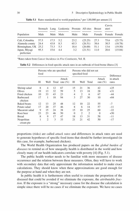
Table 5.1 shows direct age standardized incidence rates (in this case standardizedby applying the study rate to a common set of age-specific weights (world popula-tion)) and incidences of the cancers. Some of these cancers show large variations,e.g., for prostate cancer. Other cancers have much less geographical variation, e.g.,leukemia.
Descriptive data are also used to demonstrate social differences in diseases andmortality. In the UK, e.g., occupational mortality tables have been produced formore than a century. From the offices of Population Census and Surveys causes ofdeath are displayed according to occupational and social groups [2].
Table 5.2 shows cumulative incidence of symptoms of food poisoning 24 h afterhaving eaten the indicated food items. Due to tradition, these cumulative incidence
29J. Olsen et al., An Introduction to Epidemiology for Health Professionals,Springer Series on Epidemiology and Health 1, DOI 10.1007/978-1-4419-1497-2_5,C© Springer Science+Business Media, LLC 2010
30 5 Descriptive Epidemiology in Public Health
Table 5.1 Rates standardized to world population,a per 1,00,000 per annum [1]
Stomach Lung Leukemia Prostate All sites BreastCervixuteri
Population Male Male Male Male Male Female Female Female
Cali, Colombia 57.5 17.5 5.2 23.2 (25.25) 27.3 75.6 (25.75)Alameda county 24.4 43.8 8.3 65.3 (26.51) 38.6 30.5 (18.78)Birmingham, UK 25.2 73.3 5.3 18.4 (26.00) 51.1 13.6 (19.50)Japan, Miyagi
prefecture95.3 15.6 4.4 3.2 (21.51) 11.0 20.6 (15.04)
aRates taken from Cancer Incidence in Five Continents, Vol. II.
Table 5.2 Differences in food-specific attack rates in an outbreak of food-borne illness [3]
Persons who ate specifiedfood
Persons who did not eatspecified food
Ill Well TotalAttackrate (%) Ill Well Total
Attackrate (%)
Differencein attackrates
Shrimp salad 8 4 12 67 15 21 36 42 +25Olives 19 13 32 59 5 13 18 28 +31Fried chicken 10 33 43 23 4 2 6 67 –44Barbecued
chicken17 1 18 94 3 27 30 10 +84
Baked beans 12 13 25 48 12 10 22 55 –7Potato salad 17 20 37 46 8 6 14 57 –11Macaroni salad 9 15 24 38 15 10 25 60 –22Root beer 23 23 46 50 0 2 2 0 +50Bread 8 9 17 47 18 13 31 58 –11Neapolitan
cream pie1 2 3 33 21 21 42 50 –17
proportions (risks) are called attack rates and differences in attack rates are usedto generate hypotheses of specific food items that should be further investigated (inthis case, for example, barbecued chicken).
The World Health Organization has produced papers on the global burden ofdiseases to remind us of how unequally health is distributed in the world and howclosely many of our health indicators correlate with poverty [4] (Fig. 5.1).
The public health worker needs to be familiar with more measures of diseaseoccurrence and the relation between these measures. Often, they will have to workwith secondary data that only approximate the information needed to make exactcalculations. They should know when these approximations are good enough forthe purpose at hand and when they are not.
In public health it is furthermore often useful to estimate the proportion of thediseased that could be avoided if we eliminate the exposure, the attributable frac-tion. If the exposure is a “strong” necessary cause for the disease the calculation issimple since there will be no cases if we eliminate the exposure. We have no cases

5 Descriptive Epidemiology in Public Health 31
Fig. 5.1 Projected crude death rates per 100,000 by World Bank income groups for all ages, 2005and 2015 [5]
of smallpox because the smallpox virus has been eradicated, at least outside a fewlaboratories. In most other instances, the situation is more complicated. Assume wehave a fixed cohort like in Table 5.3.
Table 5.3 Obesity and fetaldeath
Obesity NFetaldeaths RR
Yes 1,000 20No 2,000 20 2.00
We could then ask ourselves how many of the 20 fetal deaths could be avoidedhad the pregnant women not been obese. Unfortunately, we have no way of know-ing that. They were obese and cannot be both obese and not obese in the samepregnancy. That is why the argument is contrary to facts – contrafactual (we cannotroll back the film and let them go through the same pregnancy without their obesity).We can, however, imagine or predict what would have occurred if they had not beenobese.
What we can do is to assume that the non-obese provide an estimate of whatwould be the risk for the obese had they not been obese – that is a very strongassumption and most likely wrong to some extent. Given we make that assumptionwe calculate that 20/2,000 × 1,000 = 10 fetal deaths would be expected among theobese had they not been obese. The attributable fraction among exposed would bethat 10 out of 20 cases could be prevented ((20 – 10)/20 = 0.50 or 50%. If we spellout how we calculated that number, it becomes

32 5 Descriptive Epidemiology in Public Health
(CI+ − CI−)1,000
CI+ × 1,000= CI+ − CI−
CI+and if you divide by the CI– you get
RR − 1
RR
CI = cumulative incidence; RR = relative risk.The attributable fraction in the entire population would be 10/40 = 0.25 or 25%;
that can be calculated as
All exposed cases(RR − 1/RR)
All cases= 20(RR − 1/RR)
40= 0.25
In this population, we estimate that it would be possible to prevent 25% (10 out of40) of all fetal deaths if we could get all obese to become normal weighted. Noticethat the attributable fraction in the population depends on the RR and the exposuredistribution in the population.
These calculations are meaningless and misleading unless we are confident thatthe associations are causal. There could be a common etiology to obesity and fetaldeath or there could be bias or other types of confounding that were not controlled inthe analysis. Attributable fractions are not measures to be used unless there is strongevidence from many sources pointing toward causal links between the exposureand the outcome. Obesity and fetal death is not yet a good candidate for calcu-lating “attributable fractions,” although it has been done. We need to know muchmore about this association before it becomes a candidate for this particular type ofmeasure.
In some textbooks you find the term etiologic fraction to mean the same as“attributable fraction.” Some use the term etiologic fraction to mean the fractionof people that had the disease because of the exposure. We need a causal conceptto understand the meaning of such a term. In our component causal model all com-ponent causes in a causal field are necessary causes within this field, but we candefine the last component cause (if it is known), the one that onsets the disease, asthe cause of interest for the etiologic fraction. Notice that if the causal field consistsof stationary genetic factors and an external toxic exposure that onsets the disease,we can emphasize this cause as we did when we said the fire was not caused by thepresence of wood but by the lighting of a match.
In this understanding, the etiologic fractions need not be of the same magnitudeas the attributable fraction. One can also imagine that the attributable fraction is 0and the etiologic fraction is greater than 0. Assume an aggressive smoking cessationprogram that works for some smokers but makes other smokers continue smokingalthough they were prepared to quit the habit. If both groups are of equal size theattributable fraction of the smoking cessation program could be 0 and the etiologicfraction is represented by those who quit smoking because of the program. Notice,
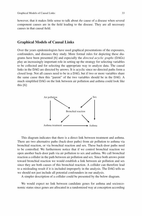
Graphical Models of Causal Links 33
however, that it makes little sense to talk about the cause of a disease when severalcomponent causes are in the field leading to the disease. They are all necessarycauses in that causal field.
Graphical Models of Causal Links
Over the years epidemiologists have used graphical presentations of the exposures,confounders, and diseases they study. More formal rules for depicting these dia-grams have been presented [6] and especially the directed acyclic graphs (DAGs)play an increasingly important role in setting up the strategy for selecting variablesto be collected and for selecting the appropriate way to analyze data. The causallinks in the DAG are directed by arrows. It is acyclic since no directed paths form aclosed loop. Not all causes need to be in a DAG, but if two or more variables sharethe same cause then this “parent” of the two variables should be in the DAG. Amuch simplified DAG on the link between air pollution and asthma could look likethis [6]:
Sex Air pollution
Bronchial reaction
Asthma Asthma treatment
This diagram indicates that there is a direct link between treatment and asthma.There are two alternative paths (back-door paths) from air pollution to asthma viabronchial reaction, or via bronchial reaction and sex. These back-door paths needto be controlled. We furthermore notice that if we control bronchial reaction weopen another back-door path via air pollution to sex and asthma. We call bronchialreaction a collider in the path between air pollution and sex. Since both arrows pointtoward bronchial reaction we would establish a link between air pollution and sexsince they are both causes of this bronchial reaction. A collider can therefore leadto a misleading result if it is included improperly in the analysis. The DAG tells uswe should not just include all potential confounders in our analysis.
A simpler description of a collider could be presented by the below diagram.
We would expect no link between candidate genes for asthma and socioeco-nomic status since genes are allocated in a randomized way at conception according

34 5 Descriptive Epidemiology in Public Health
Gene variants Socioeconomic
Status (SES)
Asthma
to Mendel’s laws. Among children with asthma you would expect an associationbetween these genetic factors and SES according to this diagram. Good socialconditions may lead to asthma as well as certain genetic factors; therefore thesetwo variables become associated in children with asthma (and to a lesser extent inchildren without asthma).
An intermediate factor is in the causal pathway from the exposure to the endpoint under study and should not be controlled in the analysis.
The causal links between a high fat diet and coronary heart diseases (CHD) couldbe like this:
High fat diet → high se-cholesterol → CHD
Including se-cholesterol would eliminate the caused association we take aninterest in. If the association is like this:
CHD High fat diet
High se-cholesterol
Genetic factors
including se-cholesterol would open a back-door path from diet to genetic factorsand CHD that cannot be controlled unless the genetic factors are measured andincluded in the model. Se-cholesterol is a collider between diet and genetic factors.Had there been no link from genetic factors to CHD, controlling for se-cholesterolwould estimate the unbroken link from diet to CHD.
DAGs have been a useful tool to clarify and communicate ideas and hypothesis.It is a tool to make predictions that can be tested and the diagram shows you how toanalyze your data. It is useful not only when a strategy for confounder adjustment isdiscussed, but also for identifying selection and information bias. The drawback is

References 35
that DAGs become very complicated in many real-life situations because the causalstructure is often complicated. Many variables are often measured by proxies (orinstrumental) variables. We may be interested in the cumulative exposure to specificcomponents of air pollution, but we may only have general data on the air qualityin the area where people live, for example. The use of instrumental variables addsto the complexity of the DAG just as including forces of selection that keep eligiblepeople out of the study tends to make DAG difficult to interpret.
For more information on DAG the reader is referred to Chapter 12 in Rothmanet al. (2008) [7].
References
1. Muir Calum, et al (eds.). Cancer Incidence in Five Continents, Volume V. IARC, Lyon, 1987.2. Occupational Health Decennial Supplement. Office for National Statistics (ONS) & Health and
Safety Executive (HSE), published every ten years, ISBN=9780116916181.3. Last JM, Wallace RB (eds.). Maxcy-Rosenau-Last. Public Health & Preventive Medicine, 13th
Edition. Appleton & Lange, Norwalk, Connecticut/San Mateo, CA, 1992.4. Lopez AD, Mathers CD, Ezzati M, Jamison DT, Murray CJL (eds.). Global Burden of Disease
and Risk Factors. Oxford University Press/The World Bank, New York/Washington, DC, 2006.5. Strong K, Mathers C, Leeder S, Beaglehole R. Preventing chronic diseases: how many lives
can we save? Lancet 2005;366(9496):1578–1582.6. Greenland S, Pearl J, Robins JM. Causal diagrams for epidemiologic research. Epidemiology
1999;10:37–48.7. Rothman KJ, Greenland S, Lash TL. Modern Epidemiology, 3rd Edition. Lippincott, Williams
and Wilkins, Philadelphia, 2008.

Chapter 6Descriptive Epidemiology in GeneticEpidemiology
Occurrence Data in Genetic Epidemiology
Genetics has come to play an increasingly important role in studies of health anddisease driven both by new technologies that enable these studies (chromosomeanalysis, DNA sequencing, genotyping) and by our recognition of the key role ofgenes and genetic variation in disease causation. Humans have 23 pairs of chro-mosomes made up of some 3 billion nucleotides (A, C, G, and T) of DNA. Thereare over 20,000 genes scattered across the human chromosomes, most containing intheir DNA sequences the information for the amino acid sequence and time/placeof expression of a particular protein. We receive one chromosome (and one copy ofeach of the genes on that chromosome) from our mother and one from our father.Variation in the DNA sequence can result in different alleles or forms of the geneand these individual differences are inherited according to Mendel’s laws of trans-mission resulting in dominant, recessive, or X-linked forms of inheritance. This vari-ation in the DNA sequence is found about once in every 1,000 nucleotides and as ofthis writing more than 5 million of these variants are well characterized. The varia-tion occurs in two common forms. The most common and studied are SNPs or singlenucleotide polymorphisms – changes in a single DNA nucleotide at a single position(A for G, for example) that are easy to characterize and enumerate. Since we havetwo copies of each chromosome, one from each parent (and each gene on those chro-mosomes), we can define a genotype as the type of each of the two possible variantswe might have (AA, AG, or GG for an A/G containing SNP). Technology allows theassay of anywhere from one to one million of these per person very cost effectively.The second common form of variation is CNVs or copy number variants wherelong segments of DNA may be present in zero to many copies. When these seg-ments include genes they can result in the absence of a gene product (if both parentscontribute zero copies) to a many-fold increase above the average amount of geneproduct if multiple gene copies are present. CNVs, while clearly of great biologicalimportance, present more challenges in analysis and are less well characterized thanSNPs as of this writing and so we will use SNPs in most examples to follow.
Many traits – from health outcomes to behavior and wealth – have a tendencyto run in families. Families share not only environmental factors (including social
37J. Olsen et al., An Introduction to Epidemiology for Health Professionals,Springer Series on Epidemiology and Health 1, DOI 10.1007/978-1-4419-1497-2_6,C© Springer Science+Business Media, LLC 2010

38 6 Descriptive Epidemiology in Genetic Epidemiology
factors), but also genetic factors. Epidemiologists have traditionally looked for envi-ronmental causes for variations in health outcomes, while geneticists have focusedon genetic factors of importance for health. The interaction between these tworesearch traditions has been surprisingly slow in emerging (the International GeneticEpidemiology Society was founded in 1991), although many researchers in bothareas agree that the determinants of most health outcomes are to be found in theinteraction between genes and environment. Not only are both genes and environ-ment etiological factors (component causes in the causal fields), but, in addition, theeffect of an environmental factor often depends on the genetic background on whichit acts, and vice versa.
Genetic factors play a central role in a broad range of monogenic diseases (i.e.,diseases caused by mutation in one gene and inherited by Mendel’s laws) from cysticfibrosis to Huntington’s disease and early-onset dementia. Most common diseases(as well as most common traits like height or eye color), however, are not mono-genic, but are more likely to be influenced by a large number of environmentaland genetic factors and their interactions. The technical development and dramaticdecline in cost have allowed genetic analyses on a minimal amount of biologicalmaterial, e.g., millions of genotypes (the genetic constitutions of the individual) canbe generated from a saliva sample or a dry spot of blood. This has been instrumen-tal in being able to incorporate genetic information into large-scale epidemiologicalstudies.
In genetic epidemiology it is studied if, how, and why some health outcomescluster in families, so some central questions are as follows:
• Does the trait or disease under study cluster in families?• Are there combinations of diseases that cluster in families?• If so, what is the relative influence of genetic and environmental factors?• What are the specific genetic variants and environmental factors influencing the
trait or disease?• How do the environmental and genetic factors interact?
In answering these questions genetic epidemiology encounters challenges knownfrom both epidemiology and genetics like heterogeneity in clinical presentation andetiology: The same disease can have a broad clinical spectrum, and the same clini-cal features can have very different etiologies. As in other epidemiological studiesit is critical that there are well-defined criteria for the disease or trait under study.Furthermore, if possible, genotyping should be done without knowledge of the dis-ease and phenotyping without information on genotypes (blinding) because both thegenotyping and the phenotyping come with some measurement errors.
Clustering of Traits and Diseases in Families
There are a number of obstacles in determining the degree of familial clusteringof a disease, in particular for diseases with manifestation late in life (e.g., demen-tia). Many family members will be too young to be at risk of having the disease,

Clustering of Traits and Diseases in Families 39
whereas others die before the typical time of diagnosis. Furthermore, in studieswhere the participant needs to return a questionnaire and participate in interviewsabout family occurrence, there is a risk that families with several affected membersare more likely to participate or be detected because these families may be particu-larly interested in studies of familial clustering of this disease. Studies of conditionsor diseases which are diagnosed early in life, and for which population-based reli-able register information exists, are less vulnerable to such biases, although they aresubject to Berkson’s bias (p. 131) if you study associations between diseases in thesame person. Clusters also occur by chance, and diseases will cluster in some fam-ilies due to chance alone. The key occurrence measure of familial clustering is therecurrence rate for different degrees of relatives to the index case, i.e., the case thatbrings the family into the study. As indicated in Fig. 6.1 such recurrence risks willbe compared with the overall population frequency in the population from whichthe cases were ascertained.
Risk in %
MZ DZ GP0
10
20
30
40
50
60
70
Fig. 6.1 Recurrence risk for relatives of an index case with cleft lip and palate [1]
The risk for the relatives is given for “zero”-degree relatives, i.e., the co-twinto a monozygotic twin (MZ) with cleft lip and palate, and similarly for first-degreerelatives (sibs including dizygotic twins (DZ), parents, and children), second-degreerelatives (grandparents, uncles, nieces, half-sibs), and third-degree relatives (e.g.,cousins). GP indicates the risk in the general population. The risk for a first-degreerelative (4%) is 40 times the risk for a random person in the general population(0.1%).
The recurrence risk is of interest in the clinical setting where questions are askedsuch as: “I have a brother with cleft lip and palate. What is the risk that my child willhave the disease?” This kind of question is classic in traditional genetic counselingfor monogenic diseases but also of importance for multifactorial diseases whichcluster in families. The recurrence risk pattern can also provide information aboutthe effect of genes: whether they act additively or multiplicatively, and how big aneffect a single gene is expected to have.

40 6 Descriptive Epidemiology in Genetic Epidemiology
The Occurrence of Genetic Diseases
Genetic disease can be used to describe a broad range of disorders from those causedby chromosome abnormalities or single-gene disruptions to complex multifactorialconditions resulting from the interplay of multiple genes and environmental factors.Single-gene disorders have a long history in public health and genetic epidemiol-ogy. Phenylketonuria (PKU) was described by Ivar Asbjørn Følling in the 1930s[2] as a recessive biochemical disorder of amino acid metabolism that, untreated,leads to profound mental retardation. Robert Guthrie [3, 4] developed a cheap andefficient test for PKU that, coupled with the recognition that an early dietary limi-tation of phenylalanine in the diet could prevent the disease manifestations, led tothe first effective population-based newborn screening tests. The PKU model is nowwidely applied throughout the developed world for a wide range of biochemicaldisorders as well as hypothyroidism and hemoglobinopathies. One hemoglobin dis-order, sickle cell anemia, was first described as a molecular disease by Linus Paulingin 1949 [5], and in the 1950s it was recognized that carriers for this autosomal reces-sive disease were resistant to falciparum Malaria while the affected homozygoteshad a high mortality in early childhood. A third common recessive disorder, cys-tic fibrosis (CF) was one of the first human disorders to have its gene identifiedusing genome mapping technologies, and the evolution of these technologies is nowenabling the application of genetic testing as one additional method available tothe epidemiologist and clinician in evaluating the role of genetic factors in diseaseetiology.
Another public health success has been the near elimination of the health con-sequences of Rhesus blood group (Rh) incompatibility between mother and fetus.An Rh+ fetus carried by an Rh– mother can induce an antibody response whichresults in the destruction of fetal red blood cells and subsequent anemia which,when severe, can result in death. Recognition of this genetic incompatibility led toprenatal screening and treatment of affected infants as well as effective preventionthrough the use of antiglobulins given to the mother during and following pregnancyto prevent the induction of the antibody response which would be exacerbated infuture pregnancies.
Prenatal testing also achieved prominence on a population scale when amniocen-tesis allowed collection of fetal cells for evaluation of chromosome anomalies suchas Trisomy 21 (Down’s syndrome). Currently such prenatal screening also includesultrasound evaluation of fetal organs and maternal serum testing to determine risksfor chromosomal aneuploidy and neural tube defects. In the aggregate these testingoptions allow a better descriptive epidemiology and introduced new screening tools.
Single-gene and chromosomal disorders are now easy to define and describewith high degrees of reliability. They are not limited to the pediatric age groups.Adult onset disorders such as the autosomal dominant cardiomyopathies or longQT syndrome have also been defined and testing has been made available. Currentmajor challenges are now focused on those more common yet complex disordersthat have an underlying genetic component but where cause may involve multi-ple genes as well as environmental triggers that make the identification of specific

References 41
risk components difficult. Disorders such as type 2 diabetes, inflammatory boweldisease, cardiovascular disease, obesity, dementia, and others are all common, yetcomplex, making genetic risk factor identification both more compelling and morechallenging. The role of the apolipoprotein E (ApoE) gene, and in particular the E4allele, in predisposing to Alzheimer’s disease, was until a few years ago one of thefew successful factor identifications to date for a common disease of adult onset.But recent successes in finding genetic risk factors for age-related macular degener-ation, type 2 diabetes, breast cancer, and myocardial infarction suggest that genomictools enable elucidation of population-based genetic risk factors. It is critical for thestudent to be aware of the ongoing developments in these areas in order to be able toprovide more effective care to patients and also to facilitate involvement of patientsin appropriate studies aimed at increasing knowledge and improving treatment. It isan area with a rapid development of technology that stretches statistical techniquesto their limit.
Common diseases can also arise as part of the expression of single-geneMendelian conditions or as a complex trait as defined above. The clinician or publichealth specialist needs to acknowledge the differences in mechanisms and implica-tions for families as well as population planning. If stroke, myocardial infarction,hypertension, cancer, or diabetes, for example, arise as part of a dominant disordertheir frequency may be much higher in an extended family than would be predictedby the prevalence of that disorder. This uneven distribution will have implicationsfor presymptomatic screening in an at-risk family and for recognizing it as a sourceof etiologic heterogeneity which will need to be incorporated into public healthplanning. In developed countries most deaths are due to cardiovascular diseasesand cancer (about one half of all deaths from these two) with accidents, diabetes,Alzheimer’s, and suicide making up other significant categories. Each of these,excepting accidents, have well-recognized genetic components whose categoriza-tion and understanding will contribute to designing better methods of preventionand treatment.
References
1. Christensen K. The 20th century Danish facial cleft population – epidemiological and genetic-epidemiological studies. Cleft Palate-Craniofac J 1999;36:96–104.
2. Følling A. Über Ausscheidung von Phenylbrenztraubensäure in den Harn alsStoffwechselanomalie in Verbindung mit Imbezillität. Hoppe-Seyler’s Zeitschrift fuerPhysiologische Chemie 1934;227:169–176.
3. Lesser AJ. Phenulketonuria and the Guthrie test. Pediatrics 1963;32:940.4. Guthrie R, Susi A. A simple phenylalanine method for detecting phenylketonuria in large
populations of newborn infants. Pediatrics 1963;32:338–343.5. Pauling I, Itano HA et al. Sickle cell anemia a molecular disease. Science 1949;110(2865):
543–548.

Chapter 7Descriptive Epidemiology in ClinicalEpidemiology
We live in the era of evidence-based medicine where “true believers” tend to disre-gard anything but randomized clinical trials (RCTs) even when assessing the impactof any intervention or diagnostic procedure. However, there are several shortcom-ings in RCTs, for instance the ability to assess long-term effects and rare outcomes.(Randomized trials are described in Chapter 9.)
Descriptive epidemiology can sometimes be used in order to assess to what extentan intervention has had an impact, especially with regard to long-term effects andoutcomes. However, such an approach is not without problems, and caution shouldbe used when minor changes in estimate of associations are used to infer causal-ity. For instance, a slight decrease in prostate cancer mortality in some populationsduring the twenty-first century, notably in the USA, has been used to “sell” the mes-sage that prostate-specific antigen (PSA) screening and/or new therapeutic strategieshave had beneficial effects. The existence of slow growing prostate cancers that willproduce no or only mild clinical symptoms within a natural life span, combinedwith differences over time in diagnostic intensity, as well as changes in the way ofreporting underlying causes of death, can at least partly explain such trends. Prostatecancer is probably the most unsuitable of all cancer forms to assess the impact ofnew interventions based on changes in incidence. This becomes evident if one com-pares temporal trends in incidence and mortality in prostate cancer between Swedenand Norway, two populations with very similar ethnic roots and lifestyles. There isa 50% higher incidence of prostate cancer as well as prostate cancer mortality inSweden than in Norway [1].
This probably mirrors differences in the diagnostic intensity with regard to theincidence but may also affect cause-specific mortality figures. It is hard to tell thedifference between dying from prostate cancer and dying with prostate cancer.
There are good uses of descriptive epidemiological data to evaluate an inter-vention. The following three different examples illustrate that – one dealing withrecommendations given to the general public, the second with screening, and thethird changes in the treatment over time.
43J. Olsen et al., An Introduction to Epidemiology for Health Professionals,Springer Series on Epidemiology and Health 1, DOI 10.1007/978-1-4419-1497-2_7,C© Springer Science+Business Media, LLC 2010

44 7 Descriptive Epidemiology in Clinical Epidemiology
Sudden Infant Death Syndrome (SIDS)
SIDS is defined as the sudden unexpected death of an infant aged younger than1 year where the circumstances of death have failed to provide a sufficient alter-native explanation. Most SIDS deaths happen within the first 8 months of life,usually around 3–4 months. Until the 1990s young mothers, male sex, pretermand/or low birth weight infants, and maternal smoking had been identified asrisk factors for SIDS and the incidence was around 2–3 per 1,000 live births.A study during the late 1980S and early 1990s from New Zealand demonstratedthat sleeping in a supine position was an independent risk factor which subsequentlyled to recommendations worldwide to parents to let their children sleep on theirbacks, as illustrated by, for instance, the “Back to Sleep” campaign in the UK in1991. The incidence of SIDS then declined dramatically during the next few years(Fig. 7.1).
Fig. 7.1 Postneonatal sudden infant death syndrome (SIDS) rates in the USA and selected othercountries, 1985–1992 [2]. These rates are calculated as the number of SIDS deaths, <27 days and<1 year of age per 1,000 live births. The 1992 SIDS rates are provisional
This drop in incidence with a 75% reduction in many different populations occur-ring about the same time following these new recommendations indicates a causallink, especially as changes in smoking habits, frequency of preterm deliveries, anddiagnostic procedures had not changed more than marginally during this relativelyshort time period.

Cytological Screening for Cervix Cancer 45
Cytological Screening for Cervix Cancer
Cancer of the cervix is one of the most common cancers in women, especiallyin developing countries, and is a major cause of premature death in middle-agedand older women. The introduction of Pap smear screening in the late 1960s wasdone in order to reduce morbidity and mortality of cervical cancer. Screeningwill lead to detection and removal of pre-malignant (cancer in situ) lesions witha simple surgical procedure, thus reducing both incidence and mortality of this can-cer. Descriptive epidemiological data were used to evaluate these programs. Datafrom Sweden, for instance, show a drop in the incidence of squamous cell can-cer of the cervix starting in the late 1960s followed by a drop in the mortalityin cervix cancer 5 years later but an increase in the incidence of cancer in situ(Fig. 7.2).
Fig. 7.2 Incidence of cancer of the cervix (ICD–7:171) [3]
These findings support a beneficial effect of this program. However, there havebeen other changes which could explain these trends, such as changes in smokinghabits, sexual education, better access to health care. To further assess the screeningprogram the incidence data can be modeled taking into account both birth cohortand time period effects (effects related to what happened during the time of birth orin the calendar time of follow-up). Since the screening procedure, in Sweden as inother countries, was primarily aimed at younger women when it was introduced inthe late 1960s, we would expect to see a decrease in birth cohorts that were offeredscreening which is seen in Fig. 7.3.
The drop in incidence of cervix cancer following the introduction of the screeningis related to a decrease in incidence in the younger birth cohorts starting in the 1930sand 1940s.

46 7 Descriptive Epidemiology in Clinical Epidemiology
Fig. 7.3 Change in incidencefor cervical cancer accordingto age in different time period[4]
Changes in Treatment of Juvenile Diabetes
Insulin treatment in juvenile diabetes was introduced in the late 1920s and diabetesnephropathy emerged as a long-term complication for these patients. Close to 50%suffer from nephropathy 20 years after starting the treatment. In the late 1960s sub-stantial changes in the treatment of juvenile diabetes were introduced. Until thena standard insulin regimen consisting of a single morning dose with a long-actinginsulin was the norm, sometimes combined with a short-acting insulin. In the 1970sa more aggressive therapy became the norm with multiple doses, which increased
Fig. 7.4 Cumulative incidence of persistent albuminuria in patients with diabetes according toduration of diabetes and calendar time of diagnosing [5]

References 47
further in the 1980s. During the same period educational programs as well as meansfor self-monitoring were added but would these new strategies have an impact onthe long-term adverse outcomes in juvenile diabetes patients?
In a study consisting of only 213 patients in a defined area in Sweden all individ-uals with juvenile diabetes diagnosed before the age of 15 were identified from1961 to 1980. Through the patient records the investigators were able to assessthe existence of persistent albuminuria, a pre-stage nephropathy, in all patients(Fig. 7.4).
Figure 7.4 shows a substantial improvement over time indicating that aggressivetreatments possibly combined with more self-care decreased persistent albuminuria.
These three examples serve to illustrate that in selected instances well-conducteddescriptive epidemiological studies can be used to evaluate new interventions,especially long-term effects and the occurrence of rare events such as SIDS.
References
1. Kvåle R, Auvinen A, Adami HO, Klint A, Hernes E, Møller B, Pukkala E, Storm HH,Tryggvadottir L, Tretli S, Wahlqvist R, Weiderpass E, Bray F. Interpreting trends inprostate cancer incidence and mortality in the five Nordic countries. J Natl Cancer Inst2007;99(24):1881–1887.
2. Willinger M, Hoffman HJ, Hartford RB. Infant sleep position and risk for sudden infant deathsyndrome: report of meeting held January 13 and 14, 1994, National Institutes of Health,Bethesda, MD. Pediatrics 1994;93(5):814–819.
3. http://www.socialstyrelsen.se/Lists/Artikelkatalog/Attachments/9325/2007-42-16_20074216.pdf
4. Gustafsson L, Pontén J, Zack M, Adami HO. International incidence rates of invasive cervi-cal cancer after introduction of cytological screening. Cancer Causes Control 1997 Sep;8(5):755–763.
5. Bojestig M, Arnqvist HJ, Hermansson G, Karlberg BE, Ludvigsson J. Declining incidence ofnephropathy in insulin-dependent diabetes mellitus. N Engl J Med 1994;330(1):15–18. Erratumin: N Engl J Med 1994 Feb 24;330(8):584.

Part IIAnalytical Epidemiology

Chapter 8Design Options
Common Designs Used to Estimate Associations
Epidemiologists use population experience to learn about associations betweenenvironmental factors, lifestyles, food intake, treatments, poverty, genes, etc., anddiseases. We do that by observing and analyzing what people do to themselves orwhat is being done to them related to the health problems they have. To be a studentof the occurrence of diseases as a function of different exposures is to be a studentof epidemiology. Since cause–effect relations unfold over time, both in terms of ageand calendar time, time plays a crucial role in these analyses and disease occur-rence is best studied from the start of exposures and in the time to follow, especiallyfor exposures that change over time, as it can be done in a follow-up study. Toobtain information on this population experience a more cost-effective strategy cansometimes be applied by sampling cases (rather than exposed and unexposed) andso-called controls. This is just another way of harvesting the underlying populationexperience as will be demonstrated later. Sometimes it may be possible for the epi-demiologist to set the conditions for exposure allocation. If we set the conditionsfor the exposure in order to learn about the health effects of these exposures, weare using an experimental design by definition, often with the intention of avoidingsome of the sources of bias that threaten many observational designs. The random-ized controlled trial is the most frequently used experimental epidemiologic design.Within these broad groups there are many variants. Most of these designs are outsidethe scope of this short introductory text.
To think about causal effects, epidemiologists often use counterfactual reasoning.Women who use hormonal drugs to treat menopausal problems have a given occur-rence of, e.g., cardiovascular diseases, but what would the occurrence have been hadthey not taken the hormones? That is of course not observable since nobody can beusing and not be using hormones at the same time, but it is possible to imagine thatthese women had not used the hormones. To estimate what the occurrence wouldhave been had they not taken the hormones, we unfortunately have to use a differ-ent group of women who did not use the hormones under study. We select thesewomen in the hope that they will provide the expected disease occurrence for theexposed, had they not been exposed. Whether we succeed or not in providing a valid
51J. Olsen et al., An Introduction to Epidemiology for Health Professionals,Springer Series on Epidemiology and Health 1, DOI 10.1007/978-1-4419-1497-2_8,C© Springer Science+Business Media, LLC 2010
52 8 Design Options
comparison group we do not and cannot know for sure. Therefore, we should notspeak lightly about causal effects but use the term associations to describe the con-trast between disease occurrence for exposed and unexposed. If we say an exposureis associated with a disease, it means just that – nothing more, nothing less; a givenexposure level has a disease occurrence that differs from what we see at anotherexposure level, in a particular data source, and that can be so for many reasons.
When we have to decide between different design options, we cannot alwaysselect the design we expect will provide the best possible counterfactual contrast.Such a design would often be the randomized controlled trial, but conducting a trialmay be out of the question for ethical reasons, or it may be impractical, too costly, ortake a long time to conduct. To evaluate the possible effect of a given screening teston long-term mortality may take decades and the screening test may be outdatedwhen results are available. For ethical reasons we cannot design an experimentalstudy to see if a given drug is fetotoxic in pregnant women, not even among womenwho have already decided to terminate their pregnancy. Over time some womenwill, however, use new drugs by accident or by choice, and we can and should tryto make the best possible use of the information they provide.
Many more aspects have to be taken into consideration when planning a studythan the quality of the designs, but if we compromise too much on quality we may bebetter off without the study. In the long run, a collection of many low-quality studiesmay cost more research money and do harm if the results are wrong. A single, largerandomized trial may be cost-effective if it is ethical and possible to do. Side effectsrelated to taking post-menopause hormones (HRT, hormonal replacement therapy)is an area where a randomized trial was long overdue when it was finally done [1].
Taking limited time and funding into consideration, the discussion on studydesign selection (from inexpensive to expensive) could go like this, using a study oncell phones and brain cancer as an example.
Ecological Study
If we had national (or regional) data on mobile phone use and brain cancer, we couldquickly produce an ecological study comparing frequencies of mobile phone use ornumber of mobile phones in use per 1,000 people and brain cancer incidence forpopulations. We may plot these data with a time lag of 5 years because we believethere will be some time lag between the exposure and disease onset. If an associationexists, we might find data like those plotted in Fig. 8.1.
Although such a graph may look convincing there are several considerations tomake: The graph is not based on individual level data and therefore does not relatecancers to individual mobile phone users. We do not know if it is the mobile phoneusers that develop cancer (the ecological fallacy). There are many other factors thatcorrelate with mobile phone use in the populations and maybe the association iscaused by these factors (confounders). Better diagnostic tools may be able to pickup cancers that were previously undetected or detected at a later stage. These better

Common Designs Used to Estimate Associations 53
Each dot represents a country or a region
IR (brain cancer)
Mobile phone use (% of users in the population, total amount of calls, etc.)
Fig. 8.1 Ecological study on mobile phone use and cancer incidence rates (IR)
diagnostic facilities may well correlate in time with mobile phone use since theyboth depend on the economic and technological developments.
We could conduct a cross-sectional study, a survey, or use data from an existinglarge ongoing survey with data on mobile phone use and brain cancer at a givenpoint in time (the time of data collection). The simplest display of such a survey issummarized in Table 8.1.
Table 8.1 A cross-sectionalstudy Mobile phone
usersBraincancer
No braincancer All
Yes a b N1No c d N0
The prevalence ratio is
PR = a/N1
c/N0
Such a survey needs to be very large to provide a reasonable number of preva-lent cases of brain cancer, and this design is a more obvious choice when both theexposure and the disease are more frequent. If we have the data and PR shows anassociation (PR>1) our concerns will be as follows:
1. We do not know the causal direction. Perhaps brain cancer leads to mobile phoneuse because patients need to be in contact with their social network. Or the oppo-site may be more likely. Brain cancer patients may isolate themselves or prefer amore personal contact than what can be achieved over the phone. The first situ-ation would produce a positive association, the latter a negative association andboth would be spurious and non-causal for the hypothesis of interest.
2. The causes of brain cancer may correlate with mobile phone use. We could takethese factors into account in the analyses if we knew them, but in this case wedo not.

54 8 Design Options
3. The reporting of mobile phone use may be in error (wrong or inaccurate) andperhaps more so for brain cancer patients, although they only report presentuse of the phones in a cross-sectional study. If mobile phone use has been awidely suggested cause of brain cancer, brain cancer patients may over-reporttheir mobile phone use in the search for an explanation of the cancer. Further,we compare recall from a sick brain with recall from a “normal” brain. In anycase, present use is only of interest if it correlates well with past use (during apossible etiologic window). The exposure data we have are not from the righttime period.
4. Not all those invited will participate in surveys. If, e.g., brain cancer patients areless likely to participate it will not in itself distort the PR, but if brain cancer caseswho are not mobile phone users more often decline to take part in the study thanbrain cancer patients who use mobile phones, an elevated PR could be a resultof this selection bias. Similar selection bias could occur among the non-braincancer patients but then it would tend to mask an association.
Case–Control Study
The next design in line to consider could be a case–control study. We select allcases of brain cancer in the population under study and a sample (controls) fromthe population that gave rise to the cases. We now record their phone use from thetime period in which we think the carcinogenic process was activated. The simplestdata lay-out would look like Table 8.2 (as in the survey, but the recording is nowlongitudinal – we try to obtain exposure data at the time period in which we believethe carcinogenic process took place, for example 5–10 years before the onset ofcancer).
Table 8.2 A case–controlstudy Exposure
history Cases Controls
Yes a bNo c d
[OR = a/c
b/d]
Depending on how controls were selected, this odds ratio (OR) could estimate theincidence rate ratio (IRR) for brain cancer among mobile phone users compared tonon-users. If this estimate is greater than 1 it would indicate an association betweenmobile phone use and brain cancer, but

Common Designs Used to Estimate Associations 55
1. Are the recalls of phone use back in time accurate and comparable for cases andcontrols? One would think that brain cancer may interfere with cognitive func-tions and thus with recall of past phone use. If cancer patients over-report phoneuse in the past (perhaps they are more sensitive to having had something closeto the brain), this could explain the observation. This source of bias is a seriousproblem, especially when the hypothesis is well known by the responders.
2. Selection bias could explain the association if exposed cases are more likely thanunexposed cases to accept an invitation to take part in the study, and that couldeasily happen if the purpose of the study is revealed at the time of recruitment.Although it is not possible to give exact guidelines on an acceptable proportionof non-responders, if but more than 30% refuse to participate selection bias is ofmajor concern. Selection bias could, however, play a role even if the proportionof non-responders is much lower, and there may be no selection bias even ifmany more refuse to take part in the study.
3. And, as before, other potential causes of brain cancer may correlate withphone use.
4. Further, a large source population is needed to provide a sufficient sample sizeto detect a small association.
Cohort Study
Next in line would be the most straightforward design, the cohort study. Selectheavy phone users and people who do not use mobile phones and follow them overtime (years or even decades). The simplest display of such a study is presented inTable 8.3.
Table 8.3 A cohort study
Exposed DiseaseObservationtime
Yes a t1No c t0
[IRR = a/t1c/t0
]
If such a study shows an IRR above 1 it would speak in favor of a causalassociation, but
1. Causes of brain cancer could correlate with mobile phone use and cause aspurious association (confounding).
2. Some of the exposure and disease data may be in error, but if brain cancer diag-nosing is made without taking phone use into consideration and phone use is

56 8 Design Options
registered before the onset of brain cancer this type of error would often leadtoward an attenuation of the IRR. And it should be possible to obtain a largeexposure contrast in countries where only part of the population uses mobilephones.
3. Although non-participation is less of a problem in the follow-up study since par-ticipants take part without knowing whether they will be brain cancer patientsor not, the selection may cause other problems. Older people may, for example,be more likely to refuse taking part in the study, reducing the number of cancerevents. If only one sex or ethnic group accepts the invitation we will have no wayof knowing if our results will apply to the people we did not recruit to the study.
4. Change of habits and phone type over time complicates the analysis, especiallyif we do not know which types of exposure to check for. Furthermore, there areother sources of radio frequency exposures in the population, although not manywith such a direct exposure to the brain.
The drawback is that you have to wait for years, perhaps decades, to get ananswer. And the study has to be large with many thousands of exposed andunexposed depending on the expected effect.
Experimental Study
If we imagine we could obtain permission and compliance to implement an experi-mental design where we decide who will be phone users and who will not (or whowill perhaps exclusively use hands-free phones that would not expose the brain andhand-held sets), we would flip a coin to let heads or tails decide whether the personwill be a phone user, or a non-user (in practice we will let a computer “flip a coin”or use another method of randomization). The display of such a study, in its simplestform, could be as in Table 8.4.
Table 8.4 A randomizedtrial
Exposure DiseaseObservationtime
Yes a t+No c t0
[IRR = a/t+c/t0
]
Should this IRR be high, it would speak quite strongly in favor of a causal asso-ciation if all participants used mobile phones according to the protocol, but resultscould still be due to chance or shortcomings in the design such as incomplete follow-up. In general, this type of design is less bias prone than other designs if complianceto phone use is kept according to the protocol, but the design is often expensive

Reference 57
because the study needs to be large with a long follow-up time, and it is often notfeasible in practice, as in this case.
In the discussed example, the ecological design will be important since even asmall increased risk in phone use will produce many new cases because the exposureis very frequent. If such a frequent exposure does not correlate with brain cancerincidences in the population, the exposure is probably not a strong cause of thedisease.
In practice, non-experimental designs are important for making new “discov-eries,” to identify new risk factors of diseases. Experimental designs are usuallyreserved to evaluate established hypotheses or to evaluate new medicines before theyare released on the market. Both observational and experimental designs are “epi-demiologic designs.” Some people have the misconception that epidemiology onlycovers non-experimental designs, but the discipline is not defined by its methods butby its subject of research.
The most important designs will be described in greater detail in the following.
Reference
1. Cuzick J. Is hormone replacement therapy safe for breast cancer patients? Editorial. JNCI2001;93(10):733.

Chapter 9Follow-Up Studies
The Non-experimental Follow-Up (Cohort) Study
If you want to study determinants (exposures) of the transition from healthy to dis-eased or death, or from diseased to non-diseased, you have to record the sequence ofcauses, treatments, and end points in time; you need to have longitudinal recordingsin most situations. If the exposure is obesity and the outcome is type 2 diabetes, youneed at least one recording of obesity in time. Obesity is defined as a body massindex (BMI) of over 30 (a man with a weight of 95 kg and a height of 1.75 m willhave a BMI of 95/1.752 = 31.0 and thus be obese).
Having identified a certain number of obese individuals (e.g., males, 40–49 yearsof age), you then follow these people for the next, say, 10 years and record the num-ber of new cases of type 2 diabetes in the cohort. Epidemiologists use the termcohort for a group of people who are followed over time (a cohort was originally aterm used in the Roman army for a subset of a legion). Say 10% develop diabetesduring the period of follow-up, the cumulative incidence (if 100 out of 1,000 obesehad type 2 diabetes) would then be 100/1,000 = 0.10 or 10%. Although this figureis useful, it does not tell us whether obesity is a risk indicator of type 2 diabetesor not. To obtain that information, you need to know what the expected cumu-lative incidence would be had the obese not been obese. That information is notavailable.
In the absence of this information, we select a group of non-obese men who webelieve have the same risk of diabetes as the obese would have had if they had notbeen obese. We would at least make sure that we select unexposed with the same agestructure and follow them over the same time period and calculate their cumulativeincidence. The more precisely we are able to formulate our hypothesis, the betterwe are able to select exposed and unexposed for the study. In the simplest versionof a cohort study, the data would look like what is displayed in Table 9.1.
Given these data we may then calculate the relative risk as
RR = (100/1,000)/(50/1,000) = 2.00
59J. Olsen et al., An Introduction to Epidemiology for Health Professionals,Springer Series on Epidemiology and Health 1, DOI 10.1007/978-1-4419-1497-2_9,C© Springer Science+Business Media, LLC 2010

60 9 Follow-Up Studies
Table 9.1 Type 2 diabetes inthe obese and non-obesecohorts Obesity N Disease
Observationyears
+ 1,000 100 9,500– 1,000 50 9,750
and the incidence rate ratio (IRR) as
IRR = (100/9,500 obs. years)/(50/9,750 obs. years) = 2.05
A relative risk may be high because the numerator is higher than the denominatoror because the denominator is much smaller than the numerator and this may beseen as a trivial fact, but the point of departure (the numerator or the denominator)may make a difference. If obesity is doubling a high disease risk, it may be moreserious from a public health point of view than if it was doubling a low risk of,say, type 1 diabetes. Type 2 diabetes is much more frequent than type 1 diabetesin most countries, and type 1 diabetes is usually a more serious disease than type 2diabetes. A doubling of the risk of type 2 diabetes would in our example mean an18% increase in absolute risk and a 0.2% increase of type 1 diabetes if the risk fornon-obese is 0.1% over the follow-up time period.
In order to provide information that illustrates actual risks, we may calculateabsolute measures of differences in risks and rates. The risk differences (RD) fortype 2 diabetes given in Table 9.1 would be
RD = (100/1,000) − (50/1,000) = 0.05
and the incidence rate difference (IRD)
IRD = (100/9,500 obs. years) − (50/9,750 obs. years) = 0.054 years−1
Studying Risk as a Function of BMI
This obesity example is a bit too simple for several reasons. Although there is anarbitrarily defined cut-off level for obesity, there is another limit for being over-weight and one for being underweight. If we think of our study as a study of fixedcohorts we would probably like to include at least three cohorts in the study: obese,overweight, and normal weight. We would then add at least one line to Table 9.1.The new table could look like Table 9.2.
Using the same comparison group – those with a normal weight – we show thatthe association may follow a dose–response pattern, and in a large sample we couldeven describe type 2 diabetes risk as a function of much finer BMI strata. If this

Studying Risk as a Function of BMI 61
Table 9.2 The risk of diabetes in obese, overweight, and normal weight cohorts
BMI Weight N Disease RR RR
30 or greater Obese 1,000 100 2.0 1.3325–29.9 Overweight 1,000 75 1.5 1 (reference)18.5–24.9 Normal 1,000 50 1.0 (reference) 0.667
association is linear, we have a constant RD across each BMI unit; the cumulativeincidence increases with a constant RD for each unit change of BMI (Fig. 9.1).
CI
BMI
Fig. 9.1 Cumulativeincidence (CI) for diabetesand BMI
Table 9.2 would follow such a structure because the risk difference is constantfrom strata to strata (0.025).
If the RR increases with a constant value across each BMI level, the associationis exponential and would look like Fig. 9.2.
BMI
3515
CIFig. 9.2 Cumulativeincidence (CI) for diabetes atBMI
Figure 9.2 illustrates a constant RR from one strata to the other. In Table 9.2the RR from normal to overweight is 1.5, but from obese to overweight it is(100/1,000)/(75/1,000) = 1.33. Had we had 112.5 diseased among the obese, theRR from overweight to obese would also be 1.5 = (112.5/1,000)/(75/1,000) andthe dose–response curve would be exponential. Figure 9.2 illustrates an exponentialcurve with an RR of 2 for each step of 5 BMI units.
If we change to logarithms of the CIs the graph between BMI and CI would againbe linear. CI increases with a fixed log RR value for each BMI level.
The log plot would look like Fig. 9.3.

62 9 Follow-Up Studies
Log CI
BMI
Fig. 9.3 Diabetes and BMI
Longitudinal Exposure Data
In our cohort design we measured BMI at a given point in time at which we also startcounting follow-up time regardless of the fact that their obesity or being overweightmay have started a long time ago. We identified a population at risk (free of diabetesat baseline) and counted observation time from the starting time. To capture changesin BMI we would need repeated (longitudinal) measures of BMI over time alongwith data on the onset of type 2 diabetes. We would then have to work on incidencerates where we calculate observation time as time being in a certain weight category.Assume Fig. 9.4 describes one man’s BMI over time.
30
25
20
3 10time
Fig. 9.4 BMI in one personover a time period of 10 years
This person would contribute 3 years of observation time within the normal BMIgroup (BMI < 25), 7 years within the overweight group (BMI 25–29), and nonewithin the obese group (BMI ≥ 30) since he only reaches this level at the end ofobservation time. We would have to repeat these BMI measurements over time forall members of the cohort to calculate incidence rates within these BMI groups. Ifthe person displayed in Fig. 9.4 got type 2 diabetes after 7 years of follow-up time,he would contribute to the incidence rate with 1/7 years in the overweight group and0/3 in the normal weight group, and these measures we have to add up for everybodyin the study. The data we get would look like what you see in Table 9.3.
This would be an appropriate way to analyze the data in lack of a specific hypoth-esis on the association between BMI and type 2 diabetes. If we had reason to expectthat there is a time lag between becoming obese and type 2 diabetes or betweena given change in weight and the disease, the calculations would be more com-plicated. In fact, there could be numerous different ways of analyzing the data,

Different Types of Cohort or Follow-Up Studies 63
Table 9.3 Incidence rates and relative incidence rates as a function of weight status
WeightObservationtime Diseased IRR
Obese t++ D++ (D++/t++)/(D0/t0)Overweight t+ D+ (D+/t+)/(D0/t0)Normal weight t0 D0 1.0 reference
and we may need rather complicated statistical techniques to perform some of theanalyses.
We also need technical skills to make the groups comparable on characteris-tics that may play a role for the risk of type 2 diabetes. Sex, age, a family historyof diabetes, diet, and physical exercise correlate with diabetes risk, and we mayneed to adjust for these factors in order to come closer to estimating unconfoundedassociations.
When we say the aim is to select unexposed with the same disease risk as exposedhad they not been exposed, we take into consideration that we do know somethingabout other risk factors that should be controlled in the analysis. Our comparisonswill not just rely on simple tabulations as those presented previously. Our com-parisons may, for example, be made within strata defined by other risk factors.A stratum of such a table could look like Table 9.4.
Table 9.4 Stratified analysis
Familyhistory Sex Age Obesity
Observationtime Disease
0 M 30–39 Yes ti+ Di+No ti– Di–
Within this stratum we compare disease occurrence among obese and non-obeseand sum up associations from all strata to make a combined estimate or that is howdata were analyzed back in time. Now stratified analyses are unfortunately too oftenreplaced with statistical modeling.
Different Types of Cohort or Follow-Up Studies
At baseline, at the start of follow-up, we may be able to classify people as exposedor unexposed. An accidental toxic exposure of short duration may leave people in alocal area exposed or unexposed. From this given point in calendar time we followup all subjects in our exposed and unexposed cohort. This we will call a fixed cohort.More often the situation will be that we start our study at a given point in calendartime and recruit eligible candidates into the study over time and move them to the

64 9 Follow-Up Studies
Start of study
E
E
E
1
2
3
4
Fig. 9.5 Observation timeaccording to exposure
exposed cohort when they become exposed, for example when they start taking anew type of medicine or move into an area with heavy air pollution (Fig. 9.5).
Eligible candidates enter our cohort at different time periods. When they becomeexposed we move them to the exposed cohort and start counting observation timefrom the time of exposure (or later if we want to take into consideration a latencytime period). Person no. 4 will thus start accumulating observation time in the unex-posed cohort (when he enters the cohort) and then change to the exposed cohortduring follow-up. In this cohort we have a dynamic recruitment to the exposedcohort during follow-up; it is a cohort with open entry. It could be a cohort ofpatients with diabetes where we may be interested in a specific new treatment asthe exposure. Since exposures may cause diseases long after exposure has stoppedwe do not always remove people from the exposed cohort when exposure stops. Ifwe did a study on car accidents and mobile phone use we would, however, removepeople from the exposed cohort when they stopped using mobile phones whiledriving. We have no reason to believe that a history of mobile phone use in itselfaffects the risk of car accidents. Such a study would have both an open entry and anopen exit.
We could also have a situation as depicted in Fig. 9.6.
E
E
E
1
2
3
Time Start of follow-up
Fig. 9.6 Observation timeaccording to exposure (E)
We would start counting observation time from the start of follow-up for personsnumbered 1 and 3 but not from the time of exposure (for no. 1). The reason is that wehave no complete surveillance of all possible eligible candidates for the study beforewe set up our follow-up surveillance program. Person number 1 is a candidate forthe study because he did not leave the region or die before the start of follow-up.

Different Types of Cohort or Follow-Up Studies 65
Some call this time from start of exposure to start of follow-up immortal observationtime because they can only enter the study if they are alive at the start of follow-up.In like manner, we start calculating observation at age 60 if we are interested inmortality rates from 60 years of age. If we take an interest in lung cancer risk forpeople who have smoked at least 40 years, we start calculating observation timewhen they have accumulated this number of exposed years.
Should we be able to identify all eligible candidates from a point dating back intime and all end points (diseases) of interest during follow-up we may reconstructobservation time back in time. We call such a study a historical cohort. This designis often used in occupational epidemiology where it may be possible to identify allfactory workers in a given plant back in time, for example based upon employmentor union records.
The terms cohort study and follow-up study are often used to describe the sametype of design although some would stress that in a cohort the aim is to follow alluntil they get the disease in question, die from other causes, or reach the date thatterminates the study. Following cancer incidence in a given region by setting upa cancer registry and counting the dynamically changing population of those whoremain within the region is therefore not a cohort study. It is a follow-up studyfor that region if we have the entire population under surveillance, but there is nointention of tracking people who leave the region.
The main design feature for a follow-up or cohort study is to select exposed andunexposed and follow disease occurrence in these groups over time. If the diseaseswe take an interest in are rare or have a long induction and latency time we may nothave the time to wait for a result or the funding needed to establish a large follow-upstudy. The case–control study then becomes an attractive alternative given certainconditions are fulfilled.
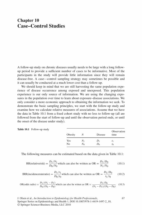
Chapter 10Case–Control Studies
A follow-up study on chronic diseases usually needs to be large with a long follow-up period to provide a sufficient number of cases to be informative. Most of theparticipants in the study will provide little information since they will remaindisease-free. A case—control sampling strategy may sometimes be possible andit can usually be conducted at a much lower cost than a follow-up.
We should keep in mind that we are still harvesting the same population expe-rience of disease occurrence among exposed and unexposed. This populationexperience is our only source of information. We are using the changing expo-sures in the population over time to learn about exposure–disease associations. Weonly consider a more economic approach to obtaining the information we seek. Todemonstrate the basic sampling principles, we start with the follow-up study andexamine how we calculate relative measures of associations. Assume that we havethe data in Table 10.1 from a fixed cohort study with no loss to follow-up (all arefollowed from the start of follow-up and until the observation period ends, or untilthe onset of the disease under study).
Table 10.1 Follow-up study
Obesity N DiseaseObservationtime
Yes N1 D1 t1No N0 D0 t0
The following measures can be estimated based on the data given in Table 10.1:
RR(relativerisk) = D1/N1
D0/N0which can also be written as OR = D1/D0
N1/N0(10.1)
IRR(incidencerateratio) = D1/t1D0/t0
which can also be written as OR = D1/D0
t1/t0(10.2)
OR(odds radio) = D1/(N1 − D1)
D0/(N0 − D0)which can also be witten as OR = D1/D0
(N1 − D1)/(N0 − D0)(10.3)
67J. Olsen et al., An Introduction to Epidemiology for Health Professionals,Springer Series on Epidemiology and Health 1, DOI 10.1007/978-1-4419-1497-2_10,C© Springer Science+Business Media, LLC 2010

68 10 Case–Control Studies
If we have no loss to follow-up we can estimate the relative risks as the ratiobetween the cumulative risks for exposed divided by the cumulative risk for theunexposed. The incidence rate ratio is in like manner based on the two incidencerates, and the odds ratio reflects the odds for disease occurrence among the exposeddivided by the disease odds among the unexposed. Notice that OR can also beexpressed as the exposure odds among diseased and the exposure odds at baselinein the entire cohort (10.1) or the odds of exposure time during follow-up (OR) orthe exposure odds among non-diseased (the right-hand side of equation 10.2). TheOR (disease odds ratio) in the cohort study is seen to be similar to the exposure oddsratio among cases and non-cases (10.3).
The rearranged right side of the equations illustrates that if we have a diseaseregister and the possibility to classify the exposure data retrospectively, we mayproduce the same relative measures of association by selecting all cases (the right-side numerators) and a sample of the denominators (right-side denominators). Toestimate relative risks we need controls to estimate the ratio of exposed and unex-posed at baseline (N1/N0). To estimate IRR we need controls to estimate the ratio ofexposed and unexposed observation time (t1/t0) and to estimate OR we need con-trols to estimate the proportion of exposed and unexposed non-diseased at the endof follow-up (N1–D1)/(N0–D0).
Assume that a follow-up study provides the results summarized in Table 10.2.
Table 10.2 Follow-up study with observation time
Obesity N Disease Observation time
Yes 10,000 200 9,900 yearsNo 30,000 300 29,850 years
Then we obtain
RR = 200/10,000
300/30,000= 2.00 (10.4)
IRR = 200/9,900
300/29,850= 2.01 (10.5)
OR = 200/9,800
300/29,700= 2.02 (10.6)
With access to a disease register for this population we may be able to identifyall cases in the population and by interviewing or by using stored biomarkers orexisting records to classify the diseased as exposed or unexposed in the proper timeperiod when the exposure may cause the disease. With the same set of cases andthree different sets of controls we can estimate RR, IRR, and OR.
We call the first type of a case–control study the case–cohort study. We selectall cases at the end of follow-up. Then we select a random sample of everybody in
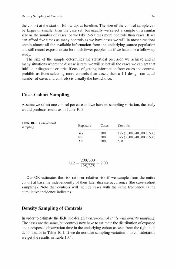
Density Sampling of Controls 69
the cohort at the start of follow-up, at baseline. The size of the control sample canbe larger or smaller than the case set, but usually we select a sample of a similarsize as the number of cases, or we take 2–5 times more controls than cases. If wecan afford five times as many controls as we have cases we will in most situationsobtain almost all the available information from the underlying source populationand still record exposure data for much fewer people than if we had done a follow-upstudy.
The size of the sample determines the statistical precision we achieve and inmany situations where the disease is rare, we will select all the cases we can get thatfulfill our diagnostic criteria. If costs of getting information from cases and controlsprohibit us from selecting more controls than cases, then a 1:1 design (an equalnumber of cases and controls) is usually the best choice.
Case–Cohort Sampling
Assume we select one control per case and we have no sampling variation, the studywould produce results as in Table 10.3.
Table 10.3 Case–cohortsampling Exposure Cases Controls
Yes 200 125 (10,000/40,000 × 500)No 300 375 (30,000/40,000 × 500)All 500 500
OR = 200/300
125/375= 2.00
Our OR estimates the risk ratio or relative risk if we sample from the entirecohort at baseline independently of their later disease occurrence (the case–cohortsampling). Note that controls will include cases with the same frequency as thecumulative incidence indicates.
Density Sampling of Controls
In order to estimate the IRR, we design a case–control study with density sampling.The cases are the same, but controls now have to estimate the distribution of exposedand unexposed observation time in the underlying cohort as seen from the right-sidedenominator in Table 10.1. If we do not take sampling variation into considerationwe get the results in Table 10.4.

70 10 Case–Control Studies
Table 10.4 Case–controlstudy with density samplingof controls
Exposure Case Controls
Yes 200 124.5 = (9,900/39,750 × 500)No 300 375.5 = (29,850/39,750 × 500)All 500 500
OR = 200/300
124.5/375.5= 2.01
One way to obtain an estimate of the exposed/unexposed observation time isto select controls at the onset of case identification. Among all in the underlyingcohort at risk of getting the disease we select controls at random at the point intime when a case is diagnosed. Thus, observation time among those at risk, whetherthey are exposed or unexposed, determines the probability of being sampled. Thissampling procedure allows controls to become cases if, after having been selectedas controls, they get the disease under study. A person may also be sampled morethan once as a control since the probability of selection is only determined by theduration of the observation time. We will estimate IRR by calculating the odds ratio(OR) in Table 10.1. This method will also work in case–control studies performedin populations that are based on a dynamic cohort if we, for example, want to studythe association between a genetic marker and childhood diabetes. We may selectpatients with newly diagnosed diabetes in our study region and among disease-freechildren at the time of diagnosis of the cases and we select controls, but this par-ticular study will be rather robust to design modifications. For example we couldsample controls at different time slots equally distributed over the time period ofcase ascertainment. Whether we allow controls to be recruited to the case group ifthey get the diagnosis under study or not is also a minor issue in this study, becausechildhood diabetes is a rare disease. Deviations from the ideal design become morecritical if we study an exposure that changes over time, like infections or air pollu-tion, or if we study a frequent disease like spontaneous abortions early in pregnancy.The principles of density sampling are illustrated in the population of 10 peoplecoming in and out of our study area during the time of case–control recruitment(Fig. 10.1).
C indicates the point in time where a participant leaves our study area, dies fromother causes, or is no longer under observation (censored). D indicates onset of thedisease under study. When person number 7 gets the disease, persons numbered 1,2, 3, 4, and 10 belong to the population at risk and are candidates for being sampledto the control set. When person number 3 becomes a case, persons numbered 1, 4,5, 8, and 10 are candidates for being sampled to the control set. If person number3 was selected as a control for case number 7 we will keep this person in the studyas both a control and a case. Since cases leave the population at risk they cannot beselected as controls from that time.

Case–Non-case Study 71
People
End recruitment Start
C
D
C
C
C
D
C
C
1
2
3
4
5
6
7
8
9
10
D = diseaseC = censored
Fig. 10.1 Follow-up of a dynamic population
Case–Non-case Study
The third type of a case–control study we will call a case–non-case study. First, weselect all the cases. Then we sample a set of controls from the non-cases at the endof follow-up. Without taking sampling variation into consideration, we end up withthe data as in Table 10.5 (sampling based on data in Table 10.2).
Table 10.5 A case–non-casestudy Exposure Cases Controls
Yes 200 124.1 = (9,800/39,500 × 500)No 300 375.9 = (29,700/39,500 × 500)All 500 500
OR = 200/300
124.1/375.9= 2.02
The exposure odds ratio equals the disease odds ratio, and odds are close toproportions (P) when the proportions (P) are small (Odds = P/(1 − P)). From thisit follows that the disease OR is close to the RR if the disease is rare among bothexposed and unexposed (as in our example). You will find this described as the raredisease assumption in many textbooks. The two other case–control designs need no

72 10 Case–Control Studies
rare disease assumptions as long as it is accepted that people may be selected morethan once to the study.
The case–non-case design was inspired by Stuart Mill’s methods of agreementand disagreement in search for causes or events [1]; we try to identify causes bylooking for similarities in exposures among cases and by trying to find what sep-arates exposures among cases from exposures among non-cases. Furthermore, thedesign leads to a simple statistical analysis since we have no overlap of cases andcontrols. The design does not take into consideration that being disease-free is aquestion of time and can lead to misleading results. Imagine, for example, that youstudy a pregnancy biomarker that changes over gestational time. If you want to seeif this biomarker is a risk factor for preterm birth you have to select controls atthe same gestational week, not women who gave birth at term (non-cases). If thebiomarker changes with gestational time, there will be a difference between casesand non-cases, even when the biomarker does not predict preterm births.
The case–control design described in this section assumes it is possible to iden-tify members of the population that gave rise to the cases and sample from them. Wealso assume that we have a disease register that captures everyone with the diseasein a given time period.
It is not always possible to identify the population at risk within some geograph-ical boundaries at given points in time. In many countries it is hardly ever possible.We may have a hospital that receives all patients with a serious disease (say, type1 diabetes) from a given catchment area. We may know the geographical bordersof this catchment area, but we may not have a list of all the people living in thisarea at a given point in time that could serve as our sampling frame. If it is out ofthe question to make a complete population registry for the entire population, wemay produce a small local population registry, for example by identifying all peopleliving within a short distance of the case person, and sample at random among thesepeople. We call these controls neighborhood controls. We may also use the case per-son’s area phone number to define the “neighborhood” and at random (random digitdialing) select a phone number within this area code that belongs to a person anduse him/her as a control. These methods may not work if we are studying exposurerelated to the close neighborhood, like air pollution and socioeconomic standards.The random digit dialing methods may be biased when having a phone, being reach-able on the phone, or having a number of phones correlate with the exposures westudy.
Patient Controls
In many case–control studies, other patients (patients with another disease than thedisease under study) are used as controls. That works well if the exposure distribu-tion among these patient controls is interchangeable with the exposure distributionamong proper controls (randomly sampled from the population that gave rise to the

Patient Controls 73
cases). The problem is that we do not know if this is the case, and it is probably sel-dom fully so. It is not so if the exposures under study cause or prevent the “control”disease. Use of other disease groups may even be biased if exposure is not causallyrelated to the control diseases but when the exposure under study correlates withthe probability of being diagnosed or hospitalized. If so, the exposure distributionwill not reflect the exposure distribution in the source population that gave rise tothe cases. Assume we take an interest in smoking as the exposure and use coloncancer controls. If coffee drinking protects against colon cancer, as some studiessuggest, colon cancer patients may have a lower smoking prevalence than what ispresent in the population that gave rise to our cases (proper controls should esti-mate that prevalence). Since smoking and coffee habits often correlate we wouldoverestimate the risk unless we adjust for coffee intake in the analyses. Assume wewant to study if a specific infection in childhood causes type 1 diabetes and we usechildren coming into the hospital with fractures as controls. If we want to study acause–effect association with short duration, this will not work. Infections tend tokeep children less active and may therefore prevent against accidents and injuries.Children with asthma may not be appropriate either since infections may initiate orworsen an asthma attack. But the design may be appropriate if we believe the infec-tion causes type 1 diabetes with a delay of months or years. Use of patient controlsmay be a useful option (and perhaps the only option) in many situations.
It may be very difficult to find a disease that for certain is neither caused norprevented by the exposure under study if the exposure interferes with several diseasemechanisms, such as infections or obesity. Studying the effect of a single gene maybe simpler, although a common gene variant like ApoE-4 is known to be associatedwith several diseases (e.g., cardiovascular diseases and Alzheimer’s disease).
There are many variations over these basic case–control designs. They all aim atharvesting the underlying population experience in order to estimate the associationbetween exposures and the disease. The most used design is the case–control studywith some type of density sampling since we rarely have the luxury of having awell-defined cohort to sample from at baseline. If we do have such a cohort we willoften use a case–cohort design, especially if you have valuable biological materialfrom the entire cohort and you intend to use this cohort to study several outcomes.A random sample from this cohort at baseline may then be used as a common setof controls for several case series. Density sampling produces one specific set ofcontrols for each case series. There is, however, one caveat when sampling controlsat baseline.
If the time between sampling of the biological material and the occurrence ofthe disease under study is not short, a slight modification is needed. Within thisfixed cohort sample you will not only sample among those that were at risk whenthe cases were diagnosed. You will also sample people who were censored beforecases surfaced to clinical detection and you have to take that into considerationwhen analyzing the data since not all were under observation for the same amountof time due to censoring. Analyzing data using survival techniques may solve theproblem.

74 10 Case–Control Studies
Secondary Identification of the Source Population
Under ideal conditions we have a disease register that captures everybody with thedisease in a given population and we are able to sample controls from this sourcepopulation and all participants in our study. These conditions are seldom if evercompletely fulfilled. Not all with the disease are diagnosed or at least not diag-nosed at the same stage of the disease. If we want to use a case–control design toestimate the effect of a newly introduced screening test the results will most likelybe misleading. The aim of the screening test is usually to diagnose a disease at anearlier stage, to bring prevalent but yet undetected patients to our attention. Untilsteady-state conditions are reached, a case–control study may show screening as arisk factor of the disease just because it moves the diagnosing forward in time.
Assume we want to study whether a given food item causes diarrhea amongtourists in Thailand. We may have to restrict our study to severe cases of diarrheathat always (or almost always) come to medical attention, but we will have no wayof identifying all tourists in Thailand at the time of data collection. Members of thesource population have to be defined by the case series as people who would becomecases if they had the disease that brought the cases to medical attention. Clearly thatis not a simple definition to use since not only the severity of the disease plays a role,but also access to health care from a practical and financial point of view. Designingcase–control studies under these conditions requires much experience [2] and shouldbe left to professional epidemiologists.
In short, the main design feature in a case–control study is the selection of casesand a random sample from the population that gave rise to the cases. The aim is toreconstruct the data we need to estimate the relative effect measures in the underly-ing population. When this is done we estimate if the exposed have the same diseaserisk as the unexposed, not if the exposure is more frequent among cases than amongcontrols. We are not comparing cases and controls but exposed and unexposed.
Case–Control Studies Using Prevalent Cases
In the described case–control designs the aim has been to provide data on factorsassociated with the transmission from healthy to diseased. The aim is to identifyincident cases and reconstruct their exposure history before the onset of the diseasewithin the time period we believe to have causal importance. Sometimes prevalentcases are recruited to a case–control study because recruitment of new cases maytake too long. If you want to study the determinants of multiple sclerosis (MS), youwould need a very large source population to obtain a sufficient number of incidentcases within a reasonable time period because the incidence rate in the population islow. Since you have MS from when you are diagnosed until you die, the prevalentpool of MS patients will be 20–40 times larger than the annual incidence, dependingupon the life expectancy of MS patients. Using prevalent cases of MS may thereforeprovide the sample size you would need, but bigger is not always better and it comeswith a price to use prevalent cases as explained in the following.

Case–Control Studies Using Prevalent Cases 75
Assume you had access to a large prevalent pool of cases from a large healthsurvey, perhaps including records of patients with diabetes. You may want to studywhether a specific genetic polymorphism is associated with diabetes, and if thisgenetic testing is expensive you might not be able to perform the test on everyonein the survey. You may select all with diabetes and then take a random sample fromall in the survey to serve as your controls. Blood samples could then be collectedand analyzed from cases and controls. The simplest display will be as presented inTable 10.6.
Table 10.6 A case–controlstudy with prevalent cases ofdiabetes
Geneticmutation Cases Controls
Yes a bNo c d
OR = a/c
b/d
This OR will estimate the prevalence proportion of diabetes among those withthe mutation divided by the prevalence proportion among those without the muta-tion, but the problem is that we use prevalence data and prevalence is a function ofincidence and disease duration. We are studying onset of diabetes or MS and sur-viving with diabetes or MS at the same time, and we cannot disentangle whether thegenetic variant increases the risk of getting the disease or whether it improves sur-vival. At least we need additional data to obtain that information, and our estimatesneed not reflect relative risks if the exposure is associated with disease duration. Ifthe exposure (a genetic variant) has prognostic implications a relative prevalencemeasure is a function of both etiologic and prognostic factors. We may get unbi-ased estimates of relative risks even when using prevalent cases if the exposuresunder study have no prognostic importance. If the genetic variant increases lifeexpectancy for MS cases, the OR would be high, even when being unrelated toincidence, and the naïve (and wrong) conclusion could be that the genetic variantcauses MS.
It may be difficult to recruit incidence cases if the disease has a high mortality,especially if you need to interview the cases. Assume that you want to study whetherphysical fitness prevents myocardial infarctions (MI) and you have to interview thecases about their physical activity in the past. You cannot interview cases in theacute phase of their MI – you have to wait until their health improves, and in thistime period the most seriously ill patients will die. Assume, for the sake of theargument, that physical exercise has no impact on the incidence of MI (it has) butimproves the prognosis (decreases short-term mortality), then the underlying cohortcould produce data as in Table 10.7.

76 10 Case–Control Studies
Table 10.7 A cohort study on physical exercise and myocardial infarctions (MI)
Physicalexercise N MI Death
Cases forinterview
Yes 10,000 50 10 40No 10,000 50 20 30
RR = 50/10,000
50/10,000= 1.0
And a case–cohort study taken from this cohort among survivors would look likeTable 10.8.
Table 10.8 A case–controlstudy based on data onsurvivors from Table 10.7
Physicalexercise Cases Controls
Yes 40 35No 30 35All 70 70
OR = 40/30
35/35= 1.33
The OR apparently wrongly indicates, according to the conditions we have set,that physical exercise increases the risk of MI. The reason is that we did not recruitall incidence cases but only the survivors. Had we recruited all incidence cases thetable would look like Table 10.9.
Table 10.9 A case–controlstudy based on data frombaseline, Table 10.7
Physicalexercise Cases Controls
Yes 50 50No 50 50All 100 100
OR = 50/50
50/50= 1.00
In principle we could have obtained unbiased results if we had included proxyresponders to replace the deceased MI patients, for example close relatives, butby doing so we rely on low-quality exposure data and may get information-biasedresults.

When to Do a Case–Control Study? 77
In brief, measures of association are based upon comparisons of disease risk forthe exposed and disease risk for the unexposed. We use the underlying populationexperience during a given follow-up period to obtain this information whether weperform a follow-up study or a case–control study. In setting up a case–control studythere are different ways of sampling this population experience depending uponwhich measure of association we take an interest in: a relative risk, incidence rateratios, or relative prevalence proportions.
When to Do a Case–Control Study?
Since case–control sampling aims at maximizing the amount of information fromthe underlying population at the lowest possible cost, the case–control study is usu-ally the design of choice if the disease under study is rare, if conditions for doingthe study are fulfilled, and if the exposure under study is not too rare. The mostimportant of these conditions is the ability to get valid exposure data on the puta-tive causes of the disease. Genetic factors that are stable over time would fulfill thiscriterion but if you take an interest in gene expression over time it may be differ-ent. It is more difficult to get valid data for exposures that change over time andespecially for exposures that have to be recalled by the participants, such as dietarydata. Eating habits change over time and cannot be recalled with any kind of preci-sion more than days or perhaps weeks back in time. It will also be difficult to recallmedicine intake back in time, unless the medicine has been used regularly over longtime periods, such as insulin. If valid records exist and are available for study, likemedical records or records of occupational exposures, these may not only replaceuncertain recalls but also provide more comparable data for cases and controls. Ina case–control study on use of mobile phones and brain cancer it will probably betoo uncertain to rely on recall of phone use back in time. The magnitude of mobilephone use is difficult to recall and it may be impossible to obtain the same degreeof accuracy in recall (symmetry in recall) among cases and controls. The cases havea disease that may interfere with cognitive functions and they may have incentivesto exaggerate phone use that are not present among controls. If billing records areavailable from phone companies, the study may provide comparable exposure dataover time and these data may be preferable although they are incomplete or evenwrong in some situations. Billing records may lack data on incoming calls and willnot indicate how the phone was used or who used it.
A case–control study is usually much more vulnerable to selection bias relatedto non-responders than a follow-up study because both the exposure and the diseasemay play a role when participants decide to accept or decline the invitation to takepart in the study. Low response rates can easily make results from a case–controlstudy unreliable and misleading.
A population-based case–control study is a study using a source populationdefined a priori by certain geographical boundaries, but if only a few of thecases accept the invitation to participate the “population-based aspect” becomes

78 10 Case–Control Studies
misleading and it may be better to let the source population be defined by the caseseries (to use a case-defined (secondary) source population).
Since sampling in a case–control study focuses upon diseased and a sample fromtheir source population, the population they came from, the case–control study usu-ally focuses on a single disease but provides an open opportunity to study a setof different exposures as putative determinants. Case–control studies are for thatreason often based on interviews using lengthy questionnaires. Genetic associationstudies usually screen for a large number of gene variants. A case–control study isa study “looking for a cause of the disease” whereas the follow-up study addressesan exposure “looking for a disease to occur.”
A case–control study has the potential of producing information much faster thana follow-up study, especially if there is a long induction and latency time betweenthe exposures and the onset of the disease. When cases and controls are recruited, theinduction and latency time is already over since you sample cases with the disease.In a cohort study with prospective data we would have to wait for this time periodto pass and therefore the exposure has to have been present in the population longenough for the exposures to cause the disease under study. If we want to studywhether a newly established technology causes cancer after 5–10 years of incubationand latency time, we may, however, do better by setting up a cohort to harvest theinformation as soon as it is available, since a case–control study cannot provide databefore the cases start to emerge from the exposure we take an interest in.
References
1. Nagel E (ed.). John Stuart Mill’s Philosophy of Scientific Method. Hafner Press, New York,1950.
2. Miettinen OS. Subject selection in case-referent studies with a secondary base. J Chronic Dis1987;40(2):186–187.

Chapter 11The Cross-Sectional Study
In a cross-sectional study, all in a given population or a random sample from thispopulation define the source population. The disease and its possible determinantsare all recorded at a given point in time. This introduces a temporal ambiguity in thepossible cause–effect association and for this reason most cross-sectional studieshave survey purposes that are only descriptive. We use cross-sectional studies toestimate, e.g., the prevalence of depression or the prevalence of having shift work.We may, however, also use the design to study stable determinants, like geneticfactors, if these factors only impact etiology and not the prognosis. Assume a cross-sectional study gives the results stated in Table 11.1.
RP = 300/2,300
700/8,700= 1.62
Table 11.1 A cross-sectional study on hormones and breast cancer
Breast cancer
Use of hormone replacement therapy (HRT) Yes No All
Yes 300 2,000 2,300No 700 8,000 8,700All 1,000 10,000 11,000
This prevalence ratio may reflect that HRT causes breast cancer or that HRTprolongs survival (improves the prognosing of breast cancer) or that breast cancerleads to an increased use of HRT (unlikely). And of course the association could becaused by bias, confounding, or chance.
Cross-sectional studies (or surveys) are important in monitoring disease frequen-cies or risk factors over time, but they play a limited role in analytical epidemiologyaddressing non-genetic determinant diseases.
When estimating disease occurrence in a cross-sectional study it should berecognized that the duration of the disease affects the probability of being sampled.A person with pneumonia lasting 10 weeks has 10 times the probability of being inthe cross-sectional sample than a person with pneumonia lasting 1 week. Prevalencedata are length biased when we compare them with incidence data.
79J. Olsen et al., An Introduction to Epidemiology for Health Professionals,Springer Series on Epidemiology and Health 1, DOI 10.1007/978-1-4419-1497-2_11,C© Springer Science+Business Media, LLC 2010

Chapter 12The Randomized Controlled Trial (RCT)
Sometimes it may be possible to set up an experimental study, especially in clini-cal epidemiology. A new treatment may be compared with the standard treatmentusing one or more features of a randomized trial. The key, and obligatory, featurein the randomized trial is randomization, which is the allocation of two (or more)treatments that are to be compared by letting this allocation depend on the resultof a random process like flipping a coin. By doing so, we let the selection of treat-ment be independent of the disease characteristics and other potential confoundingfactors. We obtain (in the long run) that the two groups will have the same treat-ment results if the two treatments are equally good or equally bad and all complywith the protocolled treatment allocation. Randomization is of crucial importance inavoiding what is called “confounding by indication” – the indication for treatmentmay confound the estimate of the treatment effect – since there are hopefully goodreasons for using one particular treatment rather than another. Randomization will,in the long run, remove confounding, including confounding by indication and con-founding by unknown factors. A perfectly designed and conducted randomized trialwill, if repeated over and over again, approach the true causal association betweenthe exposure and the disease under study. It is unfortunately much easier to designa “perfect” RCT than to conduct one.
The second element is blinding, i.e., using unlabeled treatments that cannot bedistinguished from each other. They are packed in similar containers, look alike,taste alike if they are going to be eaten, etc. Blinding is used to avoid differentialmisclassifications of, for example, side effects or treatment effects. Double blindingmeans that neither the patient nor the researcher knows which treatment has beengiven. Triple blinding indicates that also the person analyzing the data is blindeduntil all main results are estimated with coded values for treatment.
The outcome (estimated treatment effect) of a trial is a function of the natu-ral history of the disease, the possible biased reporting by the patients, doctors,and statisticians, and the possible treatment effect. Use of randomization, blinding,and placebo (an inactive treatment) or comparison with the best available treatmentmakes it possible to isolate the treatment effect. If we run a large randomized trialwhere the expected natural history of the disease does not differ between the com-pared groups and if blinding makes measurement errors similar in both groups, then
81J. Olsen et al., An Introduction to Epidemiology for Health Professionals,Springer Series on Epidemiology and Health 1, DOI 10.1007/978-1-4419-1497-2_12,C© Springer Science+Business Media, LLC 2010

82 12 The Randomized Controlled Trial (RCT)
we may be in a situation where we are entitled to say that a significant difference inprognosis probably reflects a treatment effect, but not more than that. Unfortunately,complete compliance to the protocol is seldom seen. People stop taking medicinethey do not believe works or they start taking something else.
Randomized controlled trials are usually based on informed consent, and thesequence of a trial could be as in Fig. 12.1.
Identify eligible; defined by excl./incl. criteria
Obtain informed consent
Randomize
Treatment arm Comparison arm
Non-compliance EENon-compliance
(E) endpoints/side effects
Fig. 12.1 Structure of an RCT
The randomized trial is a follow-up study where the exposed and unexposedcohorts are selected from the same pool of eligible candidates. They have the dis-ease to be treated and they are of the desired age and have other characteristicsof importance for the treatment. If they say yes to taking part in the trial (many donot), they are then randomized to one of the two (or possibly more) arms. It is impor-tant to make sure that the information fully explains the time they need to devoteto the study, the procedures they have to go through and possible risks associatedwith the treatment. During follow-up the investigator has to record compliance tothe research protocol and often an independent monitoring committee has to followpossible side effects and other deviations from the expected outcomes.
Data are then usually analyzed according to the principle we call intention to treator “as randomized so analyzed.” All comparisons are made between the randomizedgroups, regardless of whether they followed the treatment or not. The reason for notcomparing those who actually followed the protocol (this analysis is called accord-ing to protocol), is that participants made the decision to comply or not to complyand we may lose comparability obtained at randomization by the selection bias thismay entail.

12 The Randomized Controlled Trial (RCT) 83
Analyzing data according to the “intention to treat” principle is no guaranteeagainst bias when we try to estimate the treatment effects. It may, in fact, be aguarantee for bias. If a large number of people do not follow the protocol then weunderestimate the treatment effects (and side effects), and if many do not complythe comparison may be of little clinical relevance. Furthermore, intention to treatanalysis requires that we have the key endpoint data for those who left the study,which may not always be the case.
Since a randomized trial is an intervention where we impose an exposure wemust accept the responsibilities that it entails. Randomized trials are usually not anoption if we want to study harmful exposures, like an environmental exposure orrisky lifestyle factors. In order to do a trial to compare different treatments we needto be of the belief that these treatments may turn out to be equally good or bad. Ifwe believe one treatment is better than the other the trial is unethical; the principleof equipoise is then violated.
Randomized trials usually have to be relatively large to be worth doing sincesmall trials do not guarantee comparability between treatment groups. Flipping acoin 10 times only occasionally produces 50% heads and 50% tails. Flipping a coin1,000 times will yield results much closer to this expectation.
Analyzing data from a randomized trial is similar to analyzing data from anyother follow-up study measuring relative or absolute measures of association.Besides these measures, you will find a measure such as “numbers needed to treat(1 divided by the difference in risk between the two groups).” A trial on folate useto prevent neural tube defects in high-risk pregnant women showed the results givenin Table 12.1 [1].
Table 12.1 Preventing neural tube defects (NTD) by using folic acid
Exposure/folic acid Number of childrenNumber with neural tubedefects at birth
+ 593 6– 602 21
Relative prevalence ratio = 6/593
21/602= 0.29
Relative prevalence difference (RPD) = 21/602 − 6/593 = 0.025
Numbers needed to treat 1/RPD = 1/0.025 = 40
The estimates show that folate prevents a number of neural tube defects. Theprevalence proportion is about 70% lower among those who received folate thanamong those who did not (the prevalence proportion drops from 0.0035 to 0.0010).About 40 of these high-risk women (women who had a previous child with a neural

84 12 The Randomized Controlled Trial (RCT)
tube defect) have to receive folate supplementation to prevent one case with a neuraltube defect to be born – a remarkable cost-effective preventive treatment since folateis cheap and has few, if any, side effects in the doses needed to obtain a preventiveeffect [1].
Reference
1. MRC Vitamin Study Research Group. Prevention of neural tube defects: results of the MedicalResearch Council Vitamin Study. Lancet 1991;338(8760):131–137.

Chapter 13Analytical Epidemiology in Public Health
Since the public health epidemiologist focuses on determinants of disease or ways ofpreventing diseases, an experimental study is often not an option for ethical reasons,although it may be possible to remove an exposure in a randomized trial on, e.g.,smoking cessation. The public health epidemiologist will need to know more aboutnon-experimental design options and how to use available data for research. Thepublic health epidemiologist will often use secondary data (data generated for adifferent purpose, like death certificates, existing monitoring data of air pollution,employment roosters), and he or she will have to be familiar with how the data weregenerated and the limitations that may imply.
The public health epidemiologist should provide information on changes in mor-bidity and mortality and be able to address changes related to unemployment,changes in health care or rapid changes in important risk factors such as obesity,emerging epidemics, and more. It is important to have broad and general data onhealth in a population to set priorities right.
The public health epidemiologist is also expected to be able to go beyond sim-ple vital statistics and to identify patterns in morbidity or mortality that can beused to generate new hypotheses about possible causes of diseases. A public healthepidemiologist will know that a hypothesis also has to be evaluated within an epi-demiologic context. Does the disease follow a pattern that at least does not contradictthe hypothesis? If you claim that mobile phone use increases a specific form of braincancer you would at least expect this cancer to increase over time since the exposureis increasing rapidly over time. You will expect to see this increase to be strongest inage groups and populations that use the phone most often once they have accumu-lated sufficient exposure time to onset the disease. The public health epidemiologistshould also be familiar with more design options than has been described in theprevious text.
Population-based case–control sampling, for example, is difficult and vulnerableto a variety of different sources of error and the public health epidemiologist shouldknow about important design alternatives like the case-crossover study [1] that insome situations is less bias prone. The idea is simple, namely that for an exposurethat changes over time, like diet, physical exercise, and intake of medicine, individ-ual disease experience can be used to examine associations with diseases that havea short induction and latency time. The person may observe that migraine is more
85J. Olsen et al., An Introduction to Epidemiology for Health Professionals,Springer Series on Epidemiology and Health 1, DOI 10.1007/978-1-4419-1497-2_13,C© Springer Science+Business Media, LLC 2010

86 13 Analytical Epidemiology in Public Health
frequent following intake of red wine than in time periods without this exposure(the incidence rate is higher in exposed time than in unexposed time). In the case-crossover design we try to combine this experience from several people to make acommon estimate from a group of cases. A larger sample is needed if the disease israre.
The Case-Crossover Study
The case-crossover study starts with identifying cases and only cases are used (it isa case-only study). We record whether the exposure was present shortly before theonset of the disease and in a pre-specified reference time period. To make this lessabstract let us use data from a published study to illustrate the design.
Redelmeier and Tibshirani [2] took an interest in studying the associationbetween using mobile phones and car accidents. They identified drivers who hada car accident and recorded use of mobile phones in a 10-min time period lead-ing up to the accident and for a reference 10-min time period on a similar day ofthe week before. They recorded mobile phone use if the individuals were drivingand using the mobile phone at that time. Given these data, they classified all casesaccording to Table 13.1.
Table 13.1 The four possibleexposure profiles of cases Use of mobile phone
TypeReference10 min
Before accident10 min
1 Yes Yes2 Yes No3 No Yes4 No No
All information on risk comes from type 2 and type 3 people. A type 2 responseindicates a protective effect and a type 3 response a harmful effect of using the phonewhile driving. It turns out that the estimate of RR in this simple example is obtainedby calculating the total number of type 3 cases and dividing it with the total numberof type 2 cases. We use only drivers that are discordant for the exposure in the twotime periods:
RR =∑
type3∑
type2
Table 13.2 shows results from the study, and the results indicate that use ofmobile phones increases the risk of accidents about fourfold.
The table shows, perhaps as expected, that young people with short driving expe-rience have the highest relative risks of having an accident when using a mobilephone. It was more unexpected that using hands-free sets carried as high a risk as

References 87
Table 13.2 Relative risk of amotor vehicle collisionfollowing use of mobilephones, according to selectedcharacteristics [2]
CharacteristicsRelative risk (95%)confidence limits
All subjects 4.3 (3.0–6.5)
Age (year)<25 6.5 (2.2–∞)25–39 4.4 (2.8–8.8)40–54 3.6 (2.1–8.7)>55 3.3 (1.5–∞)
SexMale 4.1 (2.8–6.4)Female 4.8 (2.6–14.0)
Driving experience (year)0–9 6.2 (2.8–25.0)10–19 4.3 (2.6–10.0)20–29 3.0 (1.7–7.0)≥30 4.4 (2.1–17.0)
Type of mobile phoneHand-held 3.9 (2.7–6.1)Hands-free 5.9 (2.9–24.0)
hand-held phones. The results may even indicate that the use of hands-free sets car-ries a higher risk, but the confidence intervals (CI) show that these estimates comewith statistical uncertainties.
By making cases their own controls we adjust for all confounders that remainstable over the time period of study in this case up to a week (like driving skills orgenetic factors and in most cases car safety); we even obtain much better controlover these factors than in any other designs, including the randomized controlleddesign, and we obtain better control of genetic factors than we could obtain in atwin study. We are closer to the counterfactual ideal than in most other designs forthese time-stable factors. But there are also limitations. Were the driving conditionssimilar at the two occasions? Perhaps the use of a mobile phone was done to informabout delays and heavy traffic? These traffic conditions could be component causesof the accidents rather than phone use and of course we have to make sure that thephone calls were done before the accident and not to call for help after the accident(reverse causation).
References
1. Maclure M. The case-crossover design: a method for studying transient effects on the risk ofacute events. Am J Epidemiol 1991;133:144–153.
2. Redelmeier D, Tibshirani RJ. Association between cellular-telephone calls and motor vehiclecollisions. N Engl J Med 1997;336(7):453–458.

Chapter 14Analytical Epidemiology in GeneticEpidemiology
Disentangling the Basis for Clustering in Families
The recurrence of diseases or correlation in traits can, through studies of adoptees,twins, and half-sibs, provide information about the causes of familial clustering.Other kinds of family studies cannot separate the effect of shared environment andshared genes.
Adoption Studies
For logistic reasons, adoption studies are fewer and usually smaller than other fam-ily studies. Nevertheless, adoption studies have had a substantial impact on thenature–nurture debate for a number of traits because these studies have producedremarkable results. Adoption studies use the fact that adoptees share genetic vari-ants with their biological parents but not the parents’ environment, and they sharethe environment to some extent, but not gene variants, with their adoptive fami-lies. Among the most notable findings from adoption studies is Heston’s 1966 study[1], where he showed that among 47 children who had schizophrenic mothers andwho were put up for adoption 5 developed schizophrenia, while none of the 50control adoptees developed schizophrenia. Although the sample size is small, thestudy very convincingly indicated that schizophrenia has a strong genetic compo-nent. A strong intrauterine component could also be an explanation but twin studiesreveal much higher concordance rates in monozygotic twins compared to dizygotictwins (see below), again suggesting genetic factors as the major factor in suscep-tibility to schizophrenia [2]. Another intriguing finding that surprised many was aDanish adoption study of BMI [3]. This study showed that the BMI of adopteescorrelated more with the BMI of their biological relatives than that of their adoptiverelatives, indicating a strong genetic or early life component to variation in bodycomposition in settings with no shortage of food supply.
89J. Olsen et al., An Introduction to Epidemiology for Health Professionals,Springer Series on Epidemiology and Health 1, DOI 10.1007/978-1-4419-1497-2_14,C© Springer Science+Business Media, LLC 2010

90 14 Analytical Epidemiology in Genetic Epidemiology
Twin Studies
In humans two types of twinning occur: monozygotic (identical) twins, who shareall their genetic material, and dizygotic (fraternal) twins, who on average share 50%of their genes by descent like non-twin siblings. A twin study of a condition/diseasein its simplest form is based on a comparison of monozygotic and dizygotic concor-dance rates (i.e., the probability that a twin has the condition under study given thatthe co-twin has it), corresponding to the recurrence risk described on page 38–39.A significantly higher concordance rate in monozygotic than in dizygotic twins indi-cates that genetic factors play a role in the etiology of the disease. For continuoustraits, correlations are used instead of concordance rates. The twin study does notidentify specific genes that affect the trait but rather assesses the overall effect ofgenetic factors: the degree to which differences in the phenotype are attributable togenetic differences between people. To estimate the heritability of a trait (i.e., theproportion of the population variance attributable to genetic variation) twin data canbe analyzed using standard biometric models. A number of recent developments intwin methodology have taken place based on the incorporation of genotypes. Thisenables twin models to estimate how much of the genetic variation is due to variationin a specific gene. The classic twin methodology is based on genetic theory and thefundamental idea is that a higher degree of similarity for a trait within monozygotictwins compared to dizygotic twins is attributable to the higher degree of geneticsimilarity in monozygotic twins.
Twin studies of Alzheimer’s disease (not early onset) show that a co-twin of anaffected monozygotic twin has a 60–80% risk of becoming affected, while the risk is30–40% if the pair is dizygotic. For Parkinson’s disease the corresponding numbersare about 5% for both monozygotic and dizygotic twins. This is compatible with astrong genetic influence on Alzheimer’s disease while most etiological factors forParkinson’s disease are likely to be identified in the environment some genetic risksfor Parkinson’s disease are now known.
Twin studies are not theoretical models such as the component causal model.Under such models it is easy to argue that all diseases are 100% genetically and100% environmentally determined because it is hard to imagine any disease thatdoes not have both environmental and genetic components. However, in the practicalresearch process of identifying factors influencing disease occurrence in a givensetting at a given time the classic twin study is very useful. Twin studies can pointtoward identifiable causes of variation in a given population, e.g., to which degree itis likely that genetic differences between people play a major role for the occurrenceof that disease in that population, as seen in the Alzheimer’s disease occurrencedescribed above.
Half-Sib Studies
In countries with population registers it is possible, on a nationwide level, to iden-tify individuals who have changed their spouse or residence (or other environmental

Exposure–Disease Associations Through Studies of Relatives 91
factors). Information from these registers can be used to set up a study that is partic-ularly well suited for studying nature–nurture effects on reproductive outcomes ordiseases in early childhood [4].
Interpretation of Heritability
Twin and adoption studies suggest that a wide variety of phenotypes have a geneticcomponent to their etiology. Note that heritability estimates are time and popula-tion specific, i.e., the overall influence of genetic factors depends on the amountof environmental variance in the study population and vice versa. If, for example,more equal access to favorable living conditions and health care is introduced in apopulation, this is likely to decrease the environmental variance and hence increasethe proportion of the total variation attributable to genetic factors (the heritability).On the other hand, an increase in the environmental variance as seen in modernsocieties can also provide the opportunity for genetic effects to become expressed.
A substantial heritability for a trait suggests that it may be possible to identifyspecific genetic variants that influence the trait. The chance of identifying gene vari-ants affecting a trait through genetic association or family studies depends on thenumber of gene variants and the size of their effect.
Estimating effects in genetic epidemiology:
• What are the specific genetic variants and environmental factors influencing thetrait or disease?
• How do the environmental and genetic factors interact?
Exposure–Disease Associations Through Studies of Relatives
Nearly all lung cancers occur in smokers. Although overwhelming evidence existsfor the health-damaging effects of smoking from observational studies and animalstudies it could be claimed that what we observe is just an association betweensmoking and lung cancer and that we do not know whether it is causal or a result ofconfounding, e.g., genetic confounding. While this today may seem farfetched, oneof the leading bio-statisticians, Sir Ronald Fisher (1890–1962), actually argued thatsmoking in itself did not cause lung cancer but that certain genetic variants increasethe liability to smoke as well as the liability to develop lung cancer, and he was notalone in holding this belief at that time. Doll and Hill recognized this possibility intheir landmark paper on smoking and lung cancer from 1950 [5].
Twin studies may shed light on this hypothesis and similar (unlikely) hypothe-ses that familial-shared environmental factors would be the basis for the association.The informative twin pairs are discordant pairs, like in the case-crossover study (i.e.,twin pairs where one twin is a smoker and the other is not). If the smoking–lungcancer association is caused by genetic factors, we would not expect the smoking
92 14 Analytical Epidemiology in Genetic Epidemiology
co-twin to get lung cancer more often among monozygotic twins than the non-smoking co-twin because the two twins share all genetic factors. For dizygotictwins we would expect a weaker association than observed in the general populationbecause we partly control for genetic factors (dizygotic twins share, like siblings,about 50% of their genes). If the smoking–lung cancer association is not due togenetic or other familial factors we will expect to see that the smoking co-twinshave the highest lung cancer risk regardless of zygosity. Studies of siblings corre-spond genetically to studies of dizygotic twins. Sibling studies benefit from the factthat sibships are much more common than twins. Furthermore, many twins haveinfertile parents as twinning may be a result of infertility treatment they received,although this is only a potential problem for younger cohorts of twins.
While the above example is mostly of historic interest, this design can also beused to address some of the important contemporary topics in epidemiology: Thereis evidence that an association exists between fetal growth and later life health out-comes, such as blood pressure and cardiovascular mortality. The key question is,however, whether fetal nourishment or other factors such as genes or socioeco-nomic conditions cause the association. Some studies suggest that socioeconomicconfounding cannot explain the association between fetal growth and cardiovascu-lar mortality, but there is evidence that genetic polymorphism can affect both fetalgrowth and later insulin regulation. Analysis of twin pairs provides no strong evi-dence that the smallest twin at birth later has the highest blood pressure, suggestingthat at least part of the association can be explained by familial factors includinggenetic factors and the rearing environment [6].
Gene–Environment Interaction
It is difficult to imagine diseases that are not at least in part due to interactionsbetween genetic and environmental factors. A clear example of gene–environmentinteraction is G6PD deficiency. This is an X-linked trait of the enzyme glucose-6-phosphate dehydrogenase deficiency that facilitates energy metabolism in cells (likered blood cells) and helps protect the cell from oxidative damage. Defects in theenzyme that are genetically determined are extremely common (∼5% worldwide)and can result in hemolysis and anemia if the affected are exposed to certain nutri-tional insults such as Fava beans or pharmacologic agents including some antibioticsand antimalarials. Thus individuals with a risk genotype are normal in the absenceof an environmental exposure. This is an example where the causal field model fitsthe observation. The strength between the genetic factor and the disease dependsupon the prevalence of the dietary factors and medicine use. By avoiding theseenvironmental exposures we make sure the causal field is not completed.
Also the common ApoE-4 polymorphism, which has been shown to be a riskfactor for cardiovascular diseases and Alzheimer’s disease, seems to be involvedin gene–environment interaction making the ApoE-4 carrier more susceptible toenvironmental exposures. For example, an increased risk of chronic brain injury

Incorporation of Genetic Variables in Epidemiologic Studies 93
after head trauma has been observed for individuals who carry the ApoE-4 genevariant, compared to non-ApoE-4 carriers.
A huge challenge to gene–environment interaction studies is the multiple com-parison problem. With approximately 20,000 genes already identified, many havingseveral variants, an enormous number of possible gene–environment interactionscan be studied. One reasonable strategy is testing of biologically plausible interac-tions and replication of positive findings in large studies.
Cross-Sectional Studies of Genetic Polymorphisms
If we did not already know from vital statistics that males have substantially highermortality than females throughout life, we could get information about this froma cross-sectional population-based study. We would see that in many countries thedistribution of males to females would be approximately 1:1 at birth while it is about1:2 at age 85 and 1:4 or even 1:5 at age 100 in many settings. Similarly some geneticvariants, e.g., ApoE-4, are “weeded out” with age, indicating that they are associatedwith increased mortality. Interference from such cross-sectional studies is dependenton a stable population with little migration into the population. Remote islands willtherefore often be very well suited for such cross-sectional age-dependency studieswhile immigrant countries like the USA and Australia are less suited.
Incorporation of Genetic Variables in Epidemiologic Studies
Advances in technology frequently enable new and more powerful analyticapproaches to disease causality. While it has been possible to include variabilityin genes into studies of epidemiology since the discovery of the human blood groupantigens in the early 1900s, there has been a remarkable advance in using geneticvariables in the last few years as DNA sequencing and related technologies makeit feasible to study up to 1 million variants per individual on thousands of casesand controls at practical costs. Two general options are currently available for largeepidemiologic studies. One is directly hypothesis driven and involves choosing amodest number of variants for study when the underlying biology/physiology ofthe risk alleles is already known or highly suspected. This is called the candidategene approach and might be used in a setting of building on a known effect suchas the role of ApoE variants in dementia or cardiovascular disease or genes such asthe N-acetyltransferases that are critical in cigarette smoke detoxification. Selectingfor study variants in genes of known biological function enables the investigator toadd a powerful new variable to the analysis and limits the problems that arise frommultiple comparisons and the attendant issue of false positive results (type 1 errors).If we has no strong candidates or wishes to investigate the role of common vari-ants without a prior hypothesis as to what genes those variants might be present inone can use the genome wide association study (GWAS). In 2007 advances in both

94 14 Analytical Epidemiology in Genetic Epidemiology
technology for variant detection (a range of “DNA chips”) and analytic advances inhow to address the type 1 error problem resulted in an explosion of GWAS studiesleading to the identification possible of gene variants contributing to a wide rangeof common, complex disorders. The technology allows the study of up to 1 millionsingle nucleotide polymorphisms (SNPs) as well as 1 million copy number vari-ants (CNVs) on a single individual for less than 500 Euros. This technology takesadvantage of the observation that common human genetic variation is located inblocks where tens or even hundreds of variants in physical proximity on a chromo-some each have their individual alleles inherited in a manner highly correlated withthe alleles of nearby SNPs [7]. Thus any one SNP can serve as a surrogate markerfor many others, making it practical to provide coverage of an entire genome with afew hundred thousand SNPs and CNVs. As the cost of the assays is expected to dropfurther such approaches are now a standard tool in genetic epidemiologic studies.There are a few caveats. First, the approach is only effective when common variantscontributing to disease can be detected by virtue of their disease association. Whilethis is true for some single-gene disorders (cystic fibrosis, for example) as well ascomplex traits (breast cancer and many others) it is not true for all disorders (PKUand hypertension seem to be exceptions). In these disorders a genetic componentmay still be very active but a large number of different alleles may be contributingso that no common variant can be detected by association. These multiple allele dis-orders can be solved by DNA sequencing, and while the cost of DNA sequencingis low it remains costly enough that it is not yet in routine use for epidemiologicstudies that lack a hypothesis for a specific region to examine. Next, because ofthe enormity of the multiple comparisons (a P value of <10E-7 is required to meetBonferroni expectations) there are many signals that may require evaluation so thatreplication in independent populations for positive results is now an expectation forany such study to be accepted. Nonetheless, GWAS studies are now a component ofmost large epidemiologic efforts, and plans for obtaining material for DNA shouldbe a standard plan for any study in which a genetic variable might be active.
References
1. Heston LL. Psychiatric disorders in foster home reared children of schizophrenic mothers. Br JPsychiatry 1966;112(489):819–825.
2. Plomin R, Owen MJ, McGuffin P. The genetic basis of complex human behaviors. Science1994 Jun 17;264(5166):1733–1739. Review.
3. Sørensen TI, Holst C, Stunkard AJ. Adoption study of environmental modifications of thegenetic influences on obesity. Int Obes Relat Metab Disord 1998;22(1):73–81.
4. Olsen J, Schmidt MM, Christensen K. Evaluation of nature-nurture impact on reproductivehealth using half-siblings. Epidemiology 1997;8(1):6–11.
5. Doll R, Hill AB. Smoking and carcinoma of the lung. Br Med J 1950;4682:739–748.6. Kujala UM, Kaprio J, Koskenvuo M. Modifiable risk factors as predictors of all-cause mortality:
the roles of genetics and childhood environment. Am J Epidemiol 2002;156(11):985–993.7. Christensen K, Murray JC. What genome-wide association studies can do for medicine. N Engl
J Med 2007 Mar 15;356(11):1094–1097.

Chapter 15Analytical Epidemiology in ClinicalEpidemiology
Common Designs Used to Estimate Associations
In order to evaluate interventions or diagnostic procedures a randomized clinicaltrial (RCT) is the most accepted way. However, there are certain limitations:
1. It may be problematic to generalize the results from an RCT into normal clinicalpractice.RCTs are normally restricted to selected patient groups, often excluding chil-dren, pregnant women, and geriatric patients.
2. Long-term effects. RCTs are normally costly undertakings, which means that afollow-up exceeding 1–2 years is very uncommon and side effects may well takelonger to develop.
3. Studying rare events requires very large studies. Clinical studies encompassingmore than 500 in each arm are rare, which means that events with a frequency of1 out of 200 or less will seldom be detected in the statistical analyses.
4. Interactions with other diseases and/or other drugs, etc. Thus, in many instancesone has to use other designs in order to estimate effects or side effects.
Case-Reports and Cross-Sectional Studies
Most medical students or junior doctors will sometimes encounter a senior colleaguewho will tell her/him with conviction that once upon a time he/she had a patient whohad both diseases A and B and reacted badly to drug C and consequently treatmentD will be the only appropriate choice for this patient. The senior colleague is theninferring from a case-report, and caution is recommended. Further, results from dif-ferent cross-sectional studies have often been interpreted without taking the timesequence of events into consideration.
One example comes from the Third International Conference on PerniciousAnaemia in Stockholm in August 1937. Pernicious anemia had up to then beenregarded as a malignancy with a hematological picture impossible to distinguishfrom leukemia. Now it could be cured by giving patients B12. Dr. Birger Strandell,
95J. Olsen et al., An Introduction to Epidemiology for Health Professionals,Springer Series on Epidemiology and Health 1, DOI 10.1007/978-1-4419-1497-2_15,C© Springer Science+Business Media, LLC 2010

96 15 Analytical Epidemiology in Clinical Epidemiology
a Swedish internist, who had used data from the newly established regional can-cer registry in order to assess the long-term effects following cure for perniciousanemia, demonstrated that the patients had a very high risk for gastric cancer. Heinferred that patients with pernicious anemia were at an increased risk of gastriccancer which had clinical implications. He even had this report accepted in theJournal of Nordic Medicine (in Swedish with an abstract in German). However,the next speaker was Professor Karsner from Cleveland, Ohio, who presented theresults from a study performed at his clinic [1]. It was a cross-sectional study includ-ing more than 1,000 individuals with pernicious anemia had been diagnosed, noneof whom had gastric cancer at the time of diagnosis of pernicious anemia, and hewrote in JAMA that there was no association between pernicious anemia and gastriccancer. Although this was published before impact factors existed JAMA evidentlywas more widely read than the Journal of Nordic Medicine, and the results fromCleveland became the accepted truth until the end of the 1970s. We know now thatpernicious anemia can lead to gastric cancer, and cross-sectional studies that donot take into account the temporal dimension can produce misleading results andmisguide clinical practice.
Case–Control Studies
Screening is suitable for evaluation in observational studies, and randomized clini-cal trials will in most instances be very difficult to conduct. An RCT may provideinformation produced under ideal circumstances (efficacy) that need not representwhat happens when screening becomes a routine procedure (effectiveness). The out-come of interest is often relatively rare even in high-risk populations, and long-termeffects, often after decades, are of special interest. A good example on how to eval-uate a possible impact of screening for colorectal cancer is a study from the KaiserPermanente Medical Care program published in 1992 [2].
Two hundred and sixty-one members who died of cancer of the rectum or distalcolon between 1971 and 1988 were used as cases and 868 controls were matchedon sex and age. Sigmoidoscopy performed up to 10 years before the diagnosis ofa cancer was the screening test and the authors demonstrated a 60% reduction inmortality from rectal or distal colon cancer following screening. This reductionin mortality could be due to other exposures such as lifestyle factors or medica-tion. In order to study if confounding explained the results 268 subjects who haddied from colon cancer above the reach of sigmoidoscopy and 268 controls showedno difference in the use of sigmoidoscopy between cases and controls. Finding asimilar colon cancer mortality in these two groups indicates that intervention withsigmoidoscopy was related to this reduction in cause-specific mortality in humanswithin the reach of sigmoidoscopy. Similar results have been found in randomizedtrials.

Cohort Studies 97
Cohort Studies
A letter to the editor in 1932 [3] made the case that the adherences following aperforated appendix in females would affect their long-term fertility. The authortherefore recommended a liberal attitude for abdominal exploration at the suspi-cion of appendicitis in young females. This notion was enforced by different caseseries and became the accepted truth leading to a female predominance of appen-dectomies, especially in the younger age groups. This practice was challenged forthe first time in the 1990s in a study from Sweden [4]. Close to 10,000 women sub-jected to appendectomy under the age of 15 between 1964 and 1983 were comparedto 47,000 women who had no appendectomy before the age of 15. The authorsdemonstrated that with the exception of women who had been appendectomizedwith a normal appendix there was no difference in the fertility between those with aperforated appendix and those with an appendicitis that did not perforate (Fig. 15.1).
Fig. 15.1 Age-specific rates of first birth among women who underwent appendicectomy beforeage 15 and among age-matched controls according to life table analysis. Figure shows averagebirth rate in a given 2-year age interval
The somewhat lower age at first birth among those with a normal appendix is notsurprising as these women probably to some extent were more sexually active at anearlier age than the rest, leading to infections mimicking appendicitis. The publica-tion of this study combined with better diagnostic instruments for appendicitis hassince then resulted in a more even sex distribution among the appendectomized, forinstance in 2006 there were 5,358 appendectomies in males compared to 5,039 infemales in Sweden [5].

98 15 Analytical Epidemiology in Clinical Epidemiology
Randomized Clinical Trials (RCTs)
A randomized clinical trial is a cohort study. There is, however, one major com-ponent in the random clinical trial which gives it a certain advantage to theobservational study, namely randomization.
A correctly conducted large randomized trial will reduce confounding. If thestudy is large enough the distribution of potential confounders will be similar inboth arms.
However, two quality indicators of the study should always be assessed by thereader:
1. Analyzing data according to “intention to treat” is the key. Otherwise selectionbias will be of concern.
2. Blinding of the treatment among those assessing the outcome. Otherwise theresults can be subject to differential misclassification.
In the 1980s laparoscopic cholecystectomy surgery (surgery through a scopeto remove gallbladder stones) was introduced. This new method was deemed tobe superior with regard to the postoperative period compared to open surgery. Itwas therefore considered unethical as well as unnecessary to perform clinical tri-als. Observational studies were difficult to conduct following this procedure due toconfounding by indication, i.e., confounding by the reason for using a specific typeof surgery. The first randomized clinical trial was therefore conducted as late as in1992. Two hundred patients were included and randomization took place in the oper-ation room after which the procedure was performed either laparoscopically or asan open operation. Identical wound dressings were applied in both groups, and bothcaretakers and patients were blinded to the type of operation. Drains were usuallyremoved on the first postoperative day, patient control analgesics were discontinuedat the discretion of a patient, and oral analgesia was given if necessary. The patientswere interviewed in the out-patient clinic by a research nurse who was unaware ofthe operation procedure, and the wounds were checked by a surgeon in a separateroom. The authors demonstrated that a laparoscopic cholecystectomy takes longercompared to open surgery and does not have an advantage in terms of hospital stayor postoperative recovery. These findings were unexpected but have so far had noimpact on the patterns of operations.
In conclusion, observational studies in combination with randomized, clinicaltrials are the main method to evaluate new techniques, interventions, and diagnosticprocedures. An insightful commentary in the British Medical Journal from 1994stated the following [6]:
The view is widely held that experimental methods (randomised controlled trials) are the‘gold standard’ for evaluation and that observational methods (cohort and case control stud-ies) have little or no value. This ignores the limitations of randomised trials, which mayprove unnecessary, inappropriate, impossible, or inadequate. Many of the problems of con-ducting randomised trials could often, in theory, be overcome, but the practical implicationsfor researchers and funding bodies mean that this is often not possible. The false conflict
References 99
between those who advocate randomised trials in all situations and those who believe obser-vational data provide sufficient evidence needs to be replaced with mutual recognition ofthe complementary roles of the two approaches. Researchers should be united in their questfor scientific rigour in evaluation, regardless of the method used.
References
1. Proceedings International Society for Geographic Pathology in Stockholm 1937;303–305.2. Selby JV, Friedman GD, Quesenberry CP Jr, Weiss NS. A case-control study of screening
sigmoidoscopy and mortality from colorectal cancer. N Engl J Med 1992 Mar 5;326(10):653–657.
3. Bull P. What part is played by acute appendicitis in the causation of sterility in young girls andwomen? Acta Chir Scand 1932;71:155–165.
4. Andersson R, Lambe M, Bergström R. Fertility patterns after appendicectomy: historical cohortstudy. Br Med J 1999;318(7189):963–967.
5. Statistics from the Swedish Board of Health and Welfare 2006.6. Black N. Experimental and observational methods of evaluation. Br Med J 1994;
309(6953):540.

Part IIISources of Error

Chapter 16Confounding and Bias
In Part II we described how to estimate a measure of association between anexposure and an end point, often a disease. We are interested in “effects” but areonly able to measure associations, and we have several procedures to go throughbefore associations can be called “effects.” Measures of association emerge for allpossible reasons and only some of these relate to “effects.” Effect is a causal wordto be used with care.
It is difficult (in reality impossible) to avoid errors in large-scale population-based studies. It is especially difficult if you have not made it very clear what youwant to study and which questions you want to answer. The hypotheses should bethe guiding factor in designing the study and in deciding which data you need tocollect. The hypotheses are also key when sources of error are discussed and whenyou plan how best to avoid them. If possible you can present your hypothesis in theform of a diagram, for example a DAG. In this chapter we will consider researchbased on deduction. A hypothesis is put forward, data are collected to evaluate thishypothesis, and a conclusion is reached. A growing body of literature is, however,based on inductive inference. A large amount of data is collected without a specifichypothesis and data are analyzed to find patterns in the data structure. These studiesoften rely on powerful computer facilities and laboratory facilities without muchbiological insight. “Brutal force and ignorance” may describe the new way of ana-lyzing data. It may violate established scientific principles but sometimes producesinteresting results.
In this section of the book we will restrict our discussion to deductive studieswhere the intended study design was valid. This will limit sources of error to factorsthat can usually be classified as confounding, selection bias, or information bias.Most problems can be described under these headings, but as a reader you shouldbe aware that different terminologies are used to describe and classify sources oferror. We will therefore focus upon when and why they occur and how they causebias. There is no limit to the number of mistakes that you can make in the designphase of a study, and novel designs have to be carefully scrutinized by professionalepidemiologists and statisticians. We will leave discussions on this to the scientificliterature. We mainly consider sources of error that occur when a valid design meetsreal-world problems.
103J. Olsen et al., An Introduction to Epidemiology for Health Professionals,Springer Series on Epidemiology and Health 1, DOI 10.1007/978-1-4419-1497-2_16,C© Springer Science+Business Media, LLC 2010

104 16 Confounding and Bias
First, we should define bias, and the authorized definition [1] states
Deviation of results or inferences from the truth, or processes lead to such deviation. Anytrend in the collection, analysis, interpretation, publication, or review of data that can leadto conclusions that are systematically different from the truth.
A study is biased if it produces results that deviate from the truth due to methodproblems at any stage of research.
Some will use the term bias to include confounding – causes of the diseaseunder study that correlate with the exposure of interest. The dictionary’s definitionincludes confounding. Others will say the confounding is not an error but related tothe fact that diseases have many causes. Heavy alcohol drinkers do have a higherrisk of lung cancer. Probably not because they drink a lot, but because they oftentend to smoke. In any case, they have a high lung cancer risk. It is only wrong ifwe attribute this to their drinking habits because then we may have identified thewrong exposure. We say that the drinking exposure is confounded by its associationwith smoking habits. If they want to reduce their lung cancer risk they should stopsmoking.
Most of the measurements we make are subject to error. Recording a life timehistory of dietary habits or use of mobile phones during the last 20 years basedupon a single recording is of course more error prone than recording of age or sex.Diagnosing a disease may be easy if the disease shows clear symptoms, like measlesor bone fractures. It is more difficult to make a subtle diagnosis like attention-deficithyperactive disorder (ADHD) or to diagnose a slow growing cancer like myco-sis fungoides. If we let a number of experts diagnose the same patients they willnot always agree, even if they have access to exactly the same information. Thisinformation problem will in most cases be a source of bias we need to take intoconsideration when designing the study. Usually, we will try to design our study ina way that will allow us to know the direction of bias, perhaps even its magnitude.Many of the weak associations we find are probably weak because exposure assess-ment is too crude or too imprecise or our outcome measures are too unspecific.With better data the strength of the association may be more precisely estimated ata proper larger value.
We design our studies in the hope that those who are invited to take part in thestudy will accept the invitation, but this is seldom the case. Not all will respond,and those who do will not always remain in the study. This selection into or out ofthe study group may bias our results. It is well known among those who do surveysin order to get a representative sample of the source population that non-responderswill often make the study non-representative. If you want to estimate how many willvote for a given political party, this prediction will be wrong when it is only basedon those who responded, and it is a standard practice to adjust for non-respondingby using all available information on the non-responders to guess how they wouldhave responded.
In analytical epidemiology we are rarely interested in surveys or representa-tive samples. Surveys provide data for descriptive epidemiology. We are usually

Reference 105
interested in identifying determinants of diseases or in evaluating treatments or pre-ventive measures of diseases. Our concern is primarily devoted to how comparablethe populations are, or can be made to be, when we make inference about the deter-minants we study. We call that the internal validity of the study and we have a setof guidelines for evaluating this internal validity. We are of course also interestedin knowing if this information can be applied to other populations or future patientsand not only to the population used for sampling. We have no specific guidelines forestimating this external validity. This is an area left for common sense and futureexperience. The paradox is that we may have ways of calculating confidence limitsfor the population we used for our study, but once the study is done our interestshifts to other populations. This practice only makes sense if we believe that thecausal mechanisms are not time or population specific.
If you read papers on occupational epidemiology you will find terms like thehealthy worker effect. The term stems from situations where mortality in specificoccupations is compared with the mortality of the entire population. These workerswill often have a lower than average mortality, which is not surprising. To main-tain a full-time physically demanding job, like being a bricklayer or a carpenter,requires good health. It is not a job for those with serious physical handicaps, sothe comparison is biased. The comparison group, all in the population, does notproduce the expected mortality for workers we study had they not had the occupa-tional exposures. It is thus a type of selection bias that is within the design sphereand thus outside the sources of error we describe in this chapter. We will start withconfounding and present problems that are pertinent even in well-designed studies.
Reference
1. Last JM (ed.). A Dictionary of Epidemiology, 3rd Edition. Oxford University Press, New York,1995.

Chapter 17Confounding
A confounder is an exposure, external to our hypothesis, that biases our measureof association unless it is controlled. When we compare our exposed populationwith the unexposed comparison group the disease outcome will be different inthe two groups even if the exposed had not been exposed. The comparison isconfounded by an external factor that has to be a cause of the disease or a cor-relate for a cause of the disease. It has to be associated with the exposure understudy without being in the causal pathway between the exposure and the disease.For a schematic presentation of a simple alternative causal link between E and D(E–C–D), see Fig. 17.1.
DE
C
Fig. 17.1 Exposure (E),disease (D), and confounder(C)
If E is alcohol, D is lung cancer, and C is smoking, smoking would in manysituations confound the association E → D. Alcohol intake may be causallyrelated to smoking (probably in a more complicated way than Fig. 17.1 illus-trates) and smoking is not part of the causal pathway we take an interest in.Smoking and alcohol are expected to be associated because they may share com-mon causes such as personality, peer pressure, and a genetic predisposition foraddiction. In Fig. 17.1 the E–C–D link presents a “back-door” path between Eand D.
If E is saturated fat, D is cardiovascular diseases, and C is cholesterol, then C,or at least part of C, is not a confounder but a part of the causal path we take aninterest in (it is not just a back-door path between E and D). And the causal diagramwould be
107J. Olsen et al., An Introduction to Epidemiology for Health Professionals,Springer Series on Epidemiology and Health 1, DOI 10.1007/978-1-4419-1497-2_17,C© Springer Science+Business Media, LLC 2010

108 17 Confounding
DE
C
Notice also that the association between E and C is usually not a simple bivariateassociation but an association present after adjustment for other potential con-founders. We thus take an interest in the conditional association between E andC upon adjustment for other confounders. If we have data on both cigarette smok-ing and inhalation they need not both confound. If all cigarette smokers inhale it issufficient to adjust for smoking alone.
Table 17.1 shows strong (unusual) confounding (and effect measure modifica-tion) by sex. The female sex is a strong determinant of D, and women are much lessfrequently exposed to E than men (E is an occupational exposure). We can illustratethe association between sex and disease by stratifying our data on exposure as donein Table 17.2.
Table 17.1 A case–control study on the association between hexachlorobenzene exposure (E) andthyroid disease (D), stratified by sex [1]
Stratificationon sex E D Controls OR
Total + 8 472– 43 1,313 0.52
Men + 4 422– 1 371 3.52
Women + 4 50– 42 942 1.79
E = exposure, D = disease.
Table 17.2 Data inTable 17.1 stratified onexposure
Exposure Sex D Controls OR
Total M 5 793F 46 992 0.14
+ M 4 422F 4 50 0.12
– M 1 371F 42 942 0.06
You will rarely see confounding that changes the direction of the exposure–disease association (Table 17.1). When it happens it represents what is calledSimpson’s Paradox. Usually, confounding will attenuate or exaggerate the asso-ciation (sometimes called negative and positive confounding). A change in the

17 Confounding 109
direction of the association is unusual but possible (as in this case and in thecomparison between mortality rates in Denmark and Greenland, p. 19).
As illustrated in Fig. 17.1, we avoid confounding by eliminating the associationbetween E and C. The simplest way of eliminating this association is to restrict thestudy to a limited segment of the population that has only one category of C. IfC is age we can restrict the study to a narrow age ban. If C is sex we can restrictthe study to males or females. If C is smoking we can perform the study amongsmokers and non-smokers only. We can also design the study in such a way that noassociation exists between E and C. The random allocation of E in the randomizedtrial will usually have this effect. Since exposure is allocated randomly we wouldexpect, at least in a large trial, that the potential confounders (the determinants of thedisease we study) will be equally distributed among exposed and unexposed. We canmatch the follow-up study to make exposed and unexposed comparable concerningthe distribution of sex, age, smoking, etc., or we can control for confounding inthe analyses, given we have data on confounders, for example by stratifying theanalyses as in Table 17.1 or 17.2. Only the randomized trial will, however, adjustfor unknown confounders with some degree of certainty, a degree that is reflected inthe confidence interval.
In non-experimental studies we try to capture some of these unknown con-founders by adjusting (deconfounding) for variables that correlate with manyconditions, like sex, age, or socioeconomic status.
Confounding is a potential problem that receives much attention in most epi-demiological studies, but it is not equally serious in all studies. If you study theassociation between use of a specific component in soap and hand eczema theremay not be many correlates of this exposure that are causally linked to hand eczemaunless they are in the soap you study. If you study effects of treatment, your com-parison between treated and untreated patients may be strongly confounded by theseverity of the disease (confounding by indication for the treatment). Assuming thiscomparison is not based upon a randomization of the treatment, the two patientgroups are not expected to be comparable. Doctors are trained to select the bestpossible treatment given the state of the disease, and if they succeed in selectingthe proper candidates for treatment treated patients will not be comparable withnon-treated patients. There were reasons for using this treatment for these specificpatients, an indication for the treatment (confounding by indication). This type ofconfounding is a main reason for the need to study treatment effects in randomizedtrials. Good clinical decision making tends to ruin our options for studying treat-ment effects in non-randomized studies, and the better the clinicians are the morethey will confound our source population “by their valid indications for treatment.”
If we take an interest in a specific dietary component and its possible healtheffects, this dietary component will usually be closely linked to other dietary com-ponents. Say you take an interest in beta-carotene and its effect on lung cancer.Beta-carotene in food comes in a package, like in a carrot, and beta-carotene isjust one of many components in the carrot. Therefore, eating carrots correlates withother food components. Furthermore, people who eat carrots usually also eat othertypes of vegetables. Add to this that eating carrots replaces other types of food

110 17 Confounding
items. Adjusting for all these factors may well be impossible in a non-randomizedtrial. Studies have shown that eating a diet rich in beta-carotene is associated withlow lung cancer risks, but this association has not been found in randomized trialswhere beta-carotene was allocated by randomization. The reason could be that theprotective effect of eating carrots was not caused by beta-carotene (ecological fal-lacy) or that beta-carotene only has protective effects in combination with what elseis in the carrot. It is also possible, but not likely, that the randomized trials got it allwrong which could happen if the exposure time was too short.
The use of matching in the follow-up study is a straightforward and conceptuallysimple technique. In individual matching on, say, smoking you select an unexposedwith the same smoking history as your selected exposed (individual matching). Infrequency matching you sample unexposed so they have the same smoking frequen-cies as you have in the population of exposed. Using matching in a case–controlstudy is quite different. Matching in a case–control study does not in itself solvethe problem of confounding. The reason is that when you match cases with controlsyou change the confounder distribution among cases to make it similar to the con-founder distribution in controls (not similar among exposed and unexposed). If theexposure is a cause of the disease you introduce confounding even if there was noconfounding in the source population. If both the exposure and the confounders arecausally linked to the disease they will be associated when you stratify or match oncase status since it is a collider. If you use the terminology used in DAGs you willsee that E and C become associated when you stratify on D (match on D) since D isa collider in this diagram:
E D
C
E and C are not associated in the population. There is no arrow from C to E.In a stratified analysis with no adjustment, except the adjustment that is part of
the matched design, you have to count how many matched sets you have that followthe pattern indicated in Table 17.3 (matched sets with one case and one control).
Table 17.3 A matchedcase–control study Exposure
Type Case Control
1 0 02 + 03 0 +4 + +
+ = exposure, 0 = no exposure.

References 111
The matched sets of types 1 and 4 provide no indication of a causal association. Inall these sets neither the case nor the control is exposed [1] or they are both exposed[2]. All information is given in type 2 sets (indicating a positive association betweenexposure and disease) and type 3 sets (indicating a negative, protective, effect of theexposure). Our measure of association will simply be type 2 sets divided by type 3sets.
Any study result can always be claimed to be confounded and most study resultsare probably confounded to some extent. Still, it should be realized that confoundingneeds to be strong to explain away strong associations with a high risk ratio for thedisease.
Table 17.4 [2] shows the expected confounding effect by smoking if smokingis not adjusted for. The comparison group has the smoking prevalence shown inthe table (Exp–), and all the Exp+ groups represent different levels of confoundingby smoking among the exposed and assuming no effect of the exposure. In thistable, smoking is considered a strong risk factor with relative risks of 10 and 20.The deviations of the RR away from 1.00 are explained entirely by confoundingby smoking. As seen, smoking prevalences have to deviate substantially betweenthe compared groups to explain relative risks lower than 0.6 or higher than 1.5.Confounding by smoking cannot, under the given assumptions, explain an RR lowerthan 0.15 or higher than 3.08, even when no one or all smoke in the exposed group.
Table 17.4 How much confounding could smoking cause?
Exp
Non-smokers(1x)
Smokers(10x)
Heavysmokers(20x) RR
++
10080
–20
––
0.150.43
++
7060
3035
–5
0.570.78
– 50 40 10 1.00++
4030
4550
1520
1.221.43
+++++
2010
–––
55606525–
25303575
100
1.651.862.082.693.08
References
1. Sala M, Sunyer J, Herrero C, To-Figueras J, Grimalt J. Association between serum concentra-tions of hexachlorobenzene and polychlorobiphenyls with thyroid hormone and liver enzymesin a sample of the general population. Occup Environ Med 2001;58(3):172–177.
2. Axelson O. Confounding by smoking in occupational epidemiology. Br J Ind Med1989;46:505–507.

Chapter 18Information Bias
Most studies are based on data that are recorded with some errors. We may be able torecord gender precisely, birth weight with some errors, birth length with more errors,past occupational exposures with even more uncertainties, not to mention long-termdietary habits or use of mobile phones years ago. Sometimes diseases are diagnosedby their symptoms only, like depression. Sometimes there may be objective signs, asfor hypertension. In clinical practice, there will often be some disagreement betweengroups of clinical experts when making diagnoses. In a study we may have errors inour measurement of exposures, endpoints, and/or confounders. If these errors leadto bias (they normally will) we call this type of bias information bias. If our mea-surement is a categorical variable, such as a diagnostic code or a code for gender,we talk about misclassification or misclassification bias.
In large studies we often either have to rely on existing data or have to makeclinical tests that cannot be too invasive and often have to be inexpensive with thelimited research funds available in most countries. By comparing how a given testperforms on known cases and known non-cases diagnosed with better clinical tests(golden standard) we can quantify the amount of misclassification we may expectin the study by estimating sensitivity and specificity (Table 18.1).
Table 18.1 Applying a studytest to known cases andknown non-cases
Known disease status
Study test Cases Non-cases
Positive a bNegative c dTotal a+c b+d
The proportion of all diseased classified as test positives (cases) in the studyby the study test is a/(a+c). This is an estimate of the sensitivity of the test, theprobability of being test positive given the tested have the disease (P(test+|disease)).
The proportion of truly non-diseased we expect to classify as such in the studyusing the study test will be d/(b+d). This measure is an estimate of the specificity ofthe test, the probability of being classified as test negative given the tested do not
113J. Olsen et al., An Introduction to Epidemiology for Health Professionals,Springer Series on Epidemiology and Health 1, DOI 10.1007/978-1-4419-1497-2_18,C© Springer Science+Business Media, LLC 2010

114 18 Information Bias
have the disease (P(test–|no disease)). These estimates of sensitivity and specificitycome with some uncertainties based on who takes part in the study, which test isused, and the sample size.
If, on the other hand, we want to estimate the probability that a positive test iden-tifies a diseased we need to know the prevalence of the disease in that population, P.Given this information we can construct the probabilities of falling into the table’sfour cells, and these four probabilities are presented in Table 18.2.
Table 18.2 Probability distribution for test positives and test negatives according to diseaseoccurrence
Test Cases Non-cases All
Positive P × sens (1 – P)(1 – spec) P̂Negative P × (1 – sens) (1 – P)spec 1 − P̂All P 1 – P
Sens = sensitivity; Spec = specificity; P = prevalence proportion ofhaving the disease; P̂ = prevalence proportion of being test positive.
From Table 18.2 it is seen that the estimated prevalence P̂ is a function of the trueprevalence, P, and the sensitivity and specificity of the test [1]:
P̂ = P × sens + (1 − P)(1 − spec)
P̂ = P × sens + 1 − spec − P+ Pspec
P̂ = 1 − spec+P(sens + spec − 1)
P = P̂ + spec − 1
sens + spec − 1
Given the information on sensitivity and specificity and the proportion of testpositives we can estimate the “true” prevalence if we want to quantify the amountof bias caused by misclassification of the diseased by using an imperfect diagnosticinstrument.
Assume we have a study with complete follow-up and with no misclassificationas in Table 18.3.
Table 18.3 Follow-up studywith no diseasemisclassification
Exp N D RR
Yes 1,000 200No 1,000 100 200/1,000
100/1,000 = 2.0

18 Information Bias 115
Table 18.4 Follow-up studywith some misclassificationof the disease status
Exp N D RR
Yes 1,000 160(200 × 0.80)No 1,000 80(100 × 0.80) 160/1,000
80/1,000 = 2.0
If we now use a test to identify the diseased that has a sensitivity of 0.80 and aspecificity of 1.00 we could expect to get as in Table 18.4.
Notice that a relative measure of association is not biased by a low sensitivity inthis example as long as the sensitivity is the same in the groups to be compared.
Assume now that the sensitivity is 1.0 and the specificity is 0.90; if so we getTable 18.5.
Table 18.5 Follow-up study with misclassification of the disease status
Exp N D RR
Yes 1,000 200 + 80 (800 × 0.10)No 1,000 100 + 90 (900 × 0.10) 280/1,000
190/1,000 = 1.47
Since sensitivity and specificity are the same for exposed and unexposed we saythe misclassification is non-differential (non-differential misclassification) and asseen in this example this type of misclassification will offer bias-relative effect esti-mates toward 1. A general rule, as illustrated in this simple example, is that ratiomeasures are less sensitive to low values of sensitivity than low values of specificity.That need not be the case for absolute measures of association. The risk differencein Table 18.3 is (200/1,000 – 100/1,000) = 0.10. In Table 18.4 we get (160/1,000 –80/1,000) = 0.08. And in Table 18.5 (280/1,000 – 190/1,000) = 0.09.
If the misclassification is differential (differential misclassification), the sensitiv-ity and/or specificity differ(s) among exposed and unexposed and bias can be in anydirection.
You will often find statements in scientific papers saying that since misclassifi-cation of either exposure data or disease data was non-differential the measure ofassociation was attenuated (relative effect measures closer to 1; absolute estimatesof effect measures closer to 0). This is often overstating reality. Non-differentialmisclassification will attenuate the measure of association in most realistic situa-tions for dichotomized exposures and outcomes, but there are usually other sourcesof bias that may operate in an opposite direction and the net effect may be unknown.Bias related to non-differential misclassification will not always be toward no effect;e.g., if the disease state is wrongly coded (exposed coded 0 and unexposed coded 1where it should have been the opposite) this will produce non-differential misclas-sification that biases our measure away from the null – it will in fact reverse themeasure of association. If exposures and diseases have more than two categoriesnon-differential misclassification can in some situations bias results away from thenull. Misclassification of confounders may bias results in any direction [2].

116 18 Information Bias
In a case–control study you often identify cases from a disease register or frommedical records. Once the cases have been identified it may be possible to checkif they meet the diagnostic criteria you want them to fulfill. In cancer research it iscommon practice in high-quality case–control studies to let a reference pathologistwith known and recognized expertise go through the existing medical records andslides. Only if he/she accepts the documentation for the diagnostic criteria is thepatient admitted to the case group. The reason for this quality control is to increasethe specificity of the diagnostic procedures and to avoid the potential attenuating ofeffects by including non-cases in the case group. To see how this works, assume youhave a closed population with the following data at the end of follow-up and assumeno diagnostic uncertainties (Table 18.6).
Table 18.6 Follow-up study,no misclassification Exp N D D̄
+ 1,000 200 800– 1,000 100 900
D = disease, D̄ = no disease.
The relative risk is 2.0(
200/1,000100/1,000
)and if we sample a 1:1 case–cohort study
we will get (assuming no sampling variation and that controls reflect the exposuredistribution in the source population – 50% exposures) as in Table 18.7.
Table 18.7 Case–cohortsampling from Table 18.6 Exp Cases Controls
+ 200 150– 100 150All 300 300
OR = 200/100
150/150= 2.0
Now assume when we select the case–control study that the diagnosing is basedon diagnostic routines that have a sensitivity of 0.80 and a specificity of 0.90. Thedata in our population would then look like in Table 18.8.
Table 18.8 Follow-up study, misclassification
Exp N D̂
+ 1,000 (200 × 0.80) + (800 × 0.10) = 240– 1,000 (100 × 0.80) + (900 × 0.10) = 170RR = 760/1,000
830/1,000 = 1.41
A case–cohort sampling would give as in Table 18.9.

References 117
Table 18.9 Case–cohortsampling from Table 18.8 Exp Cases Control
+ 240 205– 170 205All 410 410
OR = 240/170
205/205= 1.41
If our reference pathologist could eliminate the false positive cases, our case–control sampling would give the result as stated in Table 18.10, given no samplingvariation.
Table 18.10 Case–cohortstudy, sampling fromTable 18.8, no false positives
Exp Cases Control
+ 160 120– 80 120All 240 240
OR = 160/80
120/120= 2.0
and we would obtain an unbiased estimate of RR (2.0).As a general rule you should try to reduce measurement errors as much as possi-
ble and what remains of measurement errors you should try to make non-differential.That can sometimes be achieved by using blinding. Make sure diagnosing is madewithout information on exposure status. When exposures are measured, for examplein the laboratory, blind the lab technicians to the disease status and make sure casesand controls are analyzed in randomly balanced sets.
References
1. Olsen J. Screening for karcinogene stoffer i arbejdsmiljøet. Kommentar (In Danish) UgeskrLæger 1978;140(51):3248–3249.
2. Greenland S. Confounding and misclassification. Am J Epidemiol 1985;122:495–506.
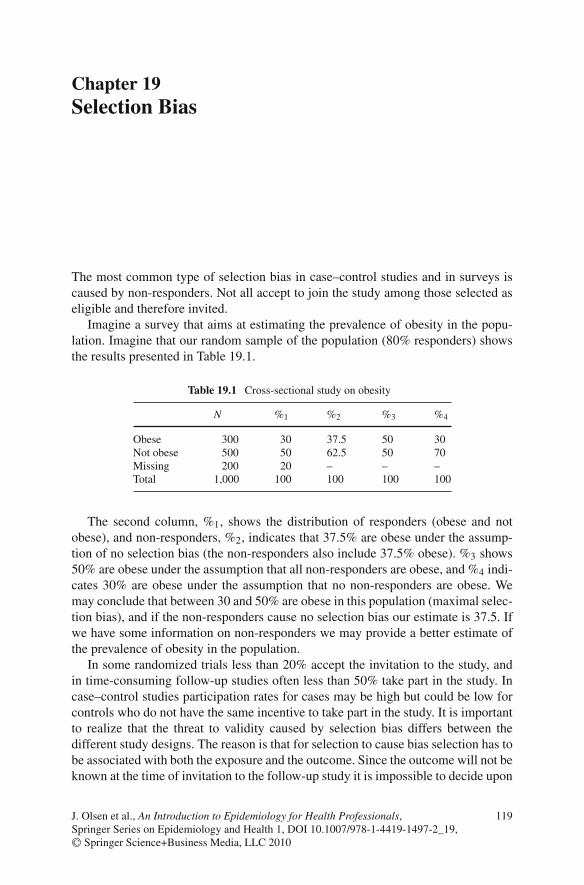
Chapter 19Selection Bias
The most common type of selection bias in case–control studies and in surveys iscaused by non-responders. Not all accept to join the study among those selected aseligible and therefore invited.
Imagine a survey that aims at estimating the prevalence of obesity in the popu-lation. Imagine that our random sample of the population (80% responders) showsthe results presented in Table 19.1.
Table 19.1 Cross-sectional study on obesity
N %1 %2 %3 %4
Obese 300 30 37.5 50 30Not obese 500 50 62.5 50 70Missing 200 20 – – –Total 1,000 100 100 100 100
The second column, %1, shows the distribution of responders (obese and notobese), and non-responders, %2, indicates that 37.5% are obese under the assump-tion of no selection bias (the non-responders also include 37.5% obese). %3 shows50% are obese under the assumption that all non-responders are obese, and %4 indi-cates 30% are obese under the assumption that no non-responders are obese. Wemay conclude that between 30 and 50% are obese in this population (maximal selec-tion bias), and if the non-responders cause no selection bias our estimate is 37.5. Ifwe have some information on non-responders we may provide a better estimate ofthe prevalence of obesity in the population.
In some randomized trials less than 20% accept the invitation to the study, andin time-consuming follow-up studies often less than 50% take part in the study. Incase–control studies participation rates for cases may be high but could be low forcontrols who do not have the same incentive to take part in the study. It is importantto realize that the threat to validity caused by selection bias differs between thedifferent study designs. The reason is that for selection to cause bias selection has tobe associated with both the exposure and the outcome. Since the outcome will not beknown at the time of invitation to the follow-up study it is impossible to decide upon
119J. Olsen et al., An Introduction to Epidemiology for Health Professionals,Springer Series on Epidemiology and Health 1, DOI 10.1007/978-1-4419-1497-2_19,C© Springer Science+Business Media, LLC 2010

120 19 Selection Bias
participation based on information that is not known at the time of recruitment. Thedecision to take part can only be associated with the outcome, through chance orthrough other variables (cause confounding). In the case–control study the situationis different. Women who have breast cancer and have used oral contraceptives (OCs)may be interested in taking part in a case–control study that aims at estimating breastcancer risk among OC users. Cancer patients or controls who never used OCs maynot have the same incentive to take part in the study.
People invited to an ongoing follow-up study cannot base their acceptance onan unknown disease they may or may not get in the future, so selection bias isless likely and the internal validity need not be influenced by the selection if thestudy is well controlled for confounding factors. However, selection may well makethe participants different from those who declined the invitation to take part in thestudy and that may often lead to a lower disease risk among the participants. This isexpected because people with poor health more often refuse to take part in researchfor various reasons. We may therefore expect a different set of confounders amongparticipants than among non-participants and we may often see less confounding inthe group that participated in the study than among all who were invited. In the ran-domized trial, selection cannot be related to exposure except by chance. Exposuresare distributed according to randomization, and outcomes are unknown at the timeof informed consent (and before randomization) but as in an observational studythose who participated may have a different disease risk than those who refused.Lack of compliance to the protocol during follow-up can and will, however, oftenlead to selection bias of the internal comparisons in a randomized trial and in otherfollow-up studies.
Selection bias in follow-up studies at baseline is mainly related to the externalvalidity or generalization of our study results. The question we have to ask our-selves is whether there are differences between the population from which we havecollected our data and the population we want to generalize to, and whether thesedifferences are expected to modify our results. (External validity is a question abouteffect measure modification.) The internal validity in a randomized trial may behigh, but the patients are usually highly selected. Will the treatment work and havethe same set of side effects for other patients?
In follow-up studies we often have to accept that participants leave the studybefore follow-up ends. In many cases, this loss to follow-up may be linked toboth the exposure and the disease under study. In a study on exposures to clean-ing agents and hand eczema, those with vulnerable skin may change jobs beforethey get eczema as a response to early markers of eczema. If all susceptible personsare removed from the exposed cohort by this self-selection a naïve analysis of datamay show the exposure to be protective. Or imagine a randomized trial for a givenpain killer. Those who remain in pain will probably be less likely to continue a treat-ment that does not work, and compliance is expected to be lower among those whoreceived such treatment. Lack of compliance to the protocol is therefore expectedto be more common in the arm of the study that receives the less effective treat-ment, and lack of compliance can eliminate some (and perhaps most) of the designbenefits achieved by the randomization.

19 Selection Bias 121
Loss to follow-up often increases with follow-up time, and a randomized trial isa less attractive study option if long-term follow-up is needed. Since selection biasduring follow-up is not unlikely the “intention to treat analyses” may remain “valid”but almost meaningless. They may provide a valid test of the null hypothesis if thestudy is powered to provide such a test, but the study provides no useful estimateof effects because the “intention to treat” correlates too little with actual treatment.The randomization is a poor instrumental variable for actual exposure.
Selection into a follow-up study only causes selection bias (it may cause con-founding) of the measure of association if the selection is associated with boththe exposure and the end point, which is unlikely, but compliance to the follow-up regime becomes very important. Lack of compliance to follow-up may well beassociated with both the exposure and the outcome. Most epidemiologists would,on the informed consent form, emphasize the importance of staying in the study ifenrolled. The advice to potential participants should in many cases be “if in doubt,stay out.”
Selection bias at recruitment is of major concern in descriptive studies and incase–control studies. If a survey aims at estimating the prevalence of ADHD andnot all in the random sample participate our estimate will be biased if the prevalenceof ADHD differs among the participants and the non-participants, which is likely.
In a case–control study (like in the follow-up study) our aim is to quantify anassociation between an exposure and a disease. That estimate is subject to selectionbias if the selection is associated with both the exposure and the disease. Since boththe exposure and the disease may be known at the time of recruitment the decisionto accept or reject the invitation can cause selection bias. If the exposure is a geneticvariant or a biomarker of an environmental pollutant the participants will usually nothave that information when they decide to take part in the study, and such a study istherefore less prone to selection bias.
Assume you want to study the association between the use of oral contraceptives(OC) and breast cancer (BC) and assume that the study would look like the data inTable 19.2 if all participated.
Table 19.2 Case–control study on the use of oral contraception (OC) and breast cancer (BC)
OC use BC Controls OR
+ 150 120– 250 280All 400 400 OR = 150/250
120/280 = 1.40
In most situations not all 800 will accept taking part in the interviewing. An80% participation rate may be considered good and 50% poor, although there are nowell-accepted cut-off points since the potential bias factor depends on many otherfactors.
Selection bias is likely because not everybody has the same incentive to partic-ipate. Women with breast cancer may find the hypothesis interesting if they haveused OCs, whereas breast cancer women who never used OCs may find it a waste
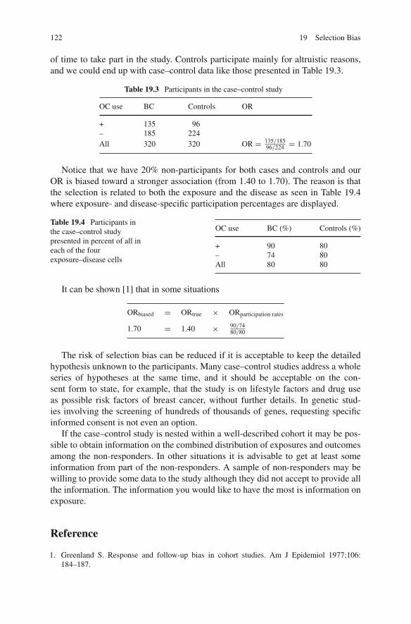
122 19 Selection Bias
of time to take part in the study. Controls participate mainly for altruistic reasons,and we could end up with case–control data like those presented in Table 19.3.
Table 19.3 Participants in the case–control study
OC use BC Controls OR
+ 135 96– 185 224All 320 320 OR = 135/185
96/224 = 1.70
Notice that we have 20% non-participants for both cases and controls and ourOR is biased toward a stronger association (from 1.40 to 1.70). The reason is thatthe selection is related to both the exposure and the disease as seen in Table 19.4where exposure- and disease-specific participation percentages are displayed.
Table 19.4 Participants inthe case–control studypresented in percent of all ineach of the fourexposure–disease cells
OC use BC (%) Controls (%)
+ 90 80– 74 80All 80 80
It can be shown [1] that in some situations
ORbiased = ORtrue × ORparticipation rates
1.70 = 1.40 × 90/7480/80
The risk of selection bias can be reduced if it is acceptable to keep the detailedhypothesis unknown to the participants. Many case–control studies address a wholeseries of hypotheses at the same time, and it should be acceptable on the con-sent form to state, for example, that the study is on lifestyle factors and drug useas possible risk factors of breast cancer, without further details. In genetic stud-ies involving the screening of hundreds of thousands of genes, requesting specificinformed consent is not even an option.
If the case–control study is nested within a well-described cohort it may be pos-sible to obtain information on the combined distribution of exposures and outcomesamong the non-responders. In other situations it is advisable to get at least someinformation from part of the non-responders. A sample of non-responders may bewilling to provide some data to the study although they did not accept to provide allthe information. The information you would like to have the most is information onexposure.
Reference
1. Greenland S. Response and follow-up bias in cohort studies. Am J Epidemiol 1977;106:184–187.

Chapter 20Making Inference and Making Decisions
The designs described in Chapter 2 allow you to estimate associations between theexposures under study and the corresponding health outcome. Making causal infer-ence is a more complicated issue. No design and no statistical procedures will inthemselves allow you to make causal inference. You can only be more or less certainabout causal relations, and making causal inference rests to some extent on subjec-tive consideration. However, the opinion of those who know the subject matter wellcarries more weight than the opinion of ignorants, although the latter could be right.History shows that the skillful more often got it right, because knowledge allows youto identify some non-causal associations. Skills will allow you to put hypotheses tocritical tests that often will reveal associations caused by bias or confounding.
Epidemiologists use terms like risk indicators to describe simple statistical asso-ciations that need not be causal. Being unmarried is a risk indicator of getting cancerof the cervix, but marital status has no direct causal link to the disease. A risk factoris a stronger term, used when we think the association could be causal but we donot really know. We may, for example, say that having frequent sex with severalpartners is a risk factor for cancer of the cervix, although we do not think that sexin itself is a risk factor. Still, we believe that if women reduce their number of sexpartners they reduce their risk of cervical cancer because having sex occasionallycarries a risk. We now have enough information to classify certain types of humanpapiloma virus transmitted by the sexual act as carcinogens because the cumula-tive documentation for a causal effect is overwhelming. Still, causal terms are to beused cautiously. Terms like etiologic fractions or attributable fractions should not beused unless we think we have a causal relation. Causal conclusions usually requiresubstantial convincing evidence from several studies.
Some hold the naïve belief that a randomized trial will provide evidence thatallows you to make causal inference, but most randomized trials have shortcomings,and even a perfect design will produce a conclusion based on statistical significancetesting that will be wrong 5% of the time if the exposure has no effect, if the nullhypothesis is true.
Making causal inference in public health and clinical practice is related to thedecision to act since there are no reasons to act on non-causal associations. Manyelements go into this decision process. First of all, we have to take into consideration
123J. Olsen et al., An Introduction to Epidemiology for Health Professionals,Springer Series on Epidemiology and Health 1, DOI 10.1007/978-1-4419-1497-2_20,C© Springer Science+Business Media, LLC 2010

124 20 Making Inference and Making Decisions
the consequences of acting on a given epidemiologic result and weigh that againstthe consequences of not acting. If we, for example, find that drinking eight cups ofcoffee per day or more during pregnancy correlates with behavioral problems in theoffspring during childhood we may decide to warn pregnant women against suchheavy coffee consumption, although we may be far from certain that the associationis causal. We are quite certain that drinking no coffee or drinking smaller amounts ofcoffee during pregnancy will cause no harm (except perhaps to the coffee producer).If we find that eating fish or sea animals during pregnancy in the Faroe Islands mayimpair brain function in the offspring, the decision process may be more difficult.If the association is strong we should warn against eating this type of food. If theassociation is weak the decision to act is more difficult. Replacing an exposure withanother may carry other health hazards and the intervention may have undesirablecultural and economic consequences. The population should of course be informedabout our findings because the final decision to act upon the results is in their hands.
Using a precautionary principle, or giving people the benefit of the doubt, maynot always be as simple as it sounds. There are some indications that the use ofmobile phones causes health problems. Should we warn people against using thesephones? We know that human life existed before the phones were invented althoughit may be hard for some to comprehend. They may carry risks when driving whiletalking on a mobile phone, but, on the other hand, the phones have uses that increasequality of life for many and they may even be used to prevent health hazards or toget help if help is needed.
In deciding when to act, causal inference is key since the causality is a necessarycondition for prevention to work; at least that prevention will lead to changes thatinclude a causal link. If we reduce the number of sexual partners we reduce therisk of HIV and cancer of the cervix because the action will eliminate some causallinks. If we had an effective vaccination program that could eliminate the causal linkbetween the virus and cancer then the behavioral changes would not be needed toreduce the cancer risk but may be needed for other reasons.
B. Hill’s causal criteria [1] state what speaks in favor of a causal effect, althoughnone of them prove causality, either taken in isolation or in combination. In fact, Hillnever used the term criteria but preferred to talk about considerations or guidelines.Whether criteria or guidelines, they are as follows:
1. Strength of association: The stronger the association, the more likely the associ-ation represents causality. Most will agree that strong associations are less likelycaused by confounding than weak associations and are therefore causal candi-dates, but strength of association provides no guarantees. Strong associationsmay be a result of bias and confounding, especially in situations where the expo-sure is part of a combined set of exposures, like when you study nicotine thatcomes together with hundreds of chemicals in tobacco smoke, caffeine that ispart of coffee, or beta-carotene that is part of certain vegetables. All these “expo-sures” correlate strongly with all other exposures in the combined package that“carries” the potential “cause.” For a confounder to explain the association itwould need to be associated with the exposures and to be causally linked to the

20 Making Inference and Making Decisions 125
outcome. Notice that in the theory of component causes the strength of an associ-ation is a function of the prevalence of the other component causes in the causalfield, leading to the disease. Obesity is a strong risk factor for diabetes in popula-tions with a high genetic susceptibility to diabetes if these genetic factors are inthe same causal field as obesity. In a population with a lower prevalence of thesegenetic factors the risk associated with obesity is expected to be lower.
2. Consistency: Consistency means that the association can be replicated. The ideais that a chance finding will usually not be replicated. The search for geneticcauses of diseases has provided many associations that could not be replicated.That is not unexpected if the prior belief is limited and many associations areexamined.
3. Specificity: A given exposure should have a specific effect according to thiscriterion. Experience shows, however, that many exposures have several healtheffects and there are often no biological reasons to expect only one. If an expo-sure during organogenesis leads to a specific malformation, like cleft lip, it may,however, raise more concern than if the exposure is related to all types of mal-formations. In the latter case, we will be more concerned about sources of biasrelated to the diagnosing of malformations or the selection of people to the study.
4. Temporality: This may be the only criterion that all would request to be fulfilled,that the cause precedes the effect. Notice that this criterion is difficult to docu-ment. Many diseases develop over long preclinical time spans and they could inthis time period impact exposures like dietary factors.
5. Biological gradient: This refers to a dose–response or dose–effect relation; thatan increasing dose leads to an increasing incidence of the disease. It is expectedthat an increasing cumulative dose leads to an increasing cumulative incidencebased on the causal fields theory. The more times you cross a street, the morelikely it is that at some point in time you will be hit by a car (that all the compo-nent causes that lead to an accident will be present). How an increasing intensityof exposure leads to a higher risk is more difficult to understand unless it isrelated to an increasing probability of the exposure to reach the target organ. Thedose–response relation may reflect an increasing number of de facto exposed athigher exposure levels.
6. Plausibility: If we understand how a given exposure causes a disease we tend tobelieve a causal explanation more than if we have no mechanistic explanation.A biological/sociological theory will also make it easier to make testable pre-dictions that can be falsified. But remember that X-rays or tobacco smoke alsocaused cancer before we knew the mechanism behind this association.
7. Coherence: This criterion is linked to the criteria of plausibility and consistency.8. Experimental evidence: If our results are supported by findings based on care-
fully controlled experiments in humans (or in animals) it speaks in favor of acausal inference.
9. Analogy: If the association we see has been found for other similar exposuresit speaks in favor of causation. Many believe that passive smoking causes lungcancer because the findings fit well with what we would expect from our studieson active smoking and our dose–response estimates.

126 20 Making Inference and Making Decisions
Most experts will use all or some of these criteria when they are to summarizeresults and make causal inference. None of these criteria, if fulfilled, will provecausality taken individually or together. Such proof does not exist. Notice that crite-ria 1, 2, and 5 deal directly with the empirical associations (epistemologic criteria).Criteria 3, 4, 6, 7, and 9 have to do with the causality itself (ontologic criteria).
Since we will never be able to prove causality we need to take action withoutsuch proof. In order to do that we often need to quantify the probability of theassociation to be causal. The International Agency for Research on Cancer (IARC)classifies possible carcinogenic exposures using different categories. Notice thatthey use strong causal language – stronger than what we recommend – probablyto advocate action where they believe action is justified. The following text is takenfrom the IARC guidelines [2]:
“Group 1 – The agent (mixture) is carcinogenic to humans.
The exposure circumstance entails exposures that are carcinogenic to humans.
This category is used when there is sufficient evidence of carcinogenicity in humans.Exceptionally, an agent (mixture) may be placed in this category when evidence of carcino-genicity in humans is less than sufficient but there is sufficient evidence of carcinogenicityin experimental animals and strong evidence in exposed humans that the agent (mixture)acts through a relevant mechanism of carcinogenicity.
Group 2
This category includes agents, mixtures and exposure circumstances for which, at oneextreme, the degree of evidence of carcinogenicity in humans is almost sufficient, as wellas those for which, at the other extreme, there are no human data but for which there isevidence of carcinogenicity in experimental animals. Agents, mixtures and exposure cir-cumstances are assigned to either group 2A (probably carcinogenic to humans) or group2B (possibly carcinogenic to humans) on the basis of epidemiological and experimentalevidence of carcinogenicity and other relevant data.
Group 2A – The agent (mixture) is probably carcinogenic to humans.
The exposure circumstance entails exposures that are probably carcinogenic to humans.
This category is used when there is limited evidence of carcinogenicity in humans and suf-ficient evidence of carcinogenicity in experimental animals and strong evidence that thecarcinogenesis is mediated by a mechanism that also operates in humans. Exceptionally, anagent, mixture or exposure circumstance may be classified in this category solely on thebasis of limited evidence of carcinogenicity in humans.
Group 2B – The agent (mixture) is possibly carcinogenic to humans.
The exposure circumstance entails exposures that are possibly carcinogenic to humans.
This category is used for agents, mixtures and exposure circumstances for which there islimited evidence of carcinogenicity in humans and less than sufficient evidence of carcino-genicity in experimental animals. It may also be used when there is inadequate evidence ofcarcinogenicity in humans but there is sufficient evidence of carcinogenicity in experimentalanimals. In some instances, an agent, mixture or exposure circumstance for which there isinadequate evidence of carcinogenicity in humans but limited evidence of carcinogenicityin experimental animals together with supporting evidence from other relevant data may beplaced in this group.

References 127
Group 3 – The agent (mixture or exposure circumstance) is not classifiable as to itscarcinogenicity to humans.
This category is used most commonly for agents, mixtures and exposure circumstances forwhich the evidence of carcinogenicity is inadequate in humans and inadequate or limitedin experimental animals. Exceptionally, agents (mixtures) for which the evidence of car-cinogenicity is inadequate in humans but sufficient in experimental animals may be placedin this category when there is strong evidence that the mechanism of carcinogenicity inexperimental animals does not operate in humans.
Agents, mixtures and exposure circumstances that do not fall into any other group are alsoplaced in this category.
Group 4 – The agent (mixture) is probably not carcinogenic to humans.
This category is used for agents or mixtures for which there is evidence suggesting lackof carcinogenicity in humans and in experimental animals. In some instances, agents ormixtures for which there is inadequate evidence of carcinogenicity in humans but evi-dence suggesting lack of carcinogenicity in experimental animals, consistently and stronglysupported by a broad range of other relevant data, may be classified in this group” [3].
These guidelines illustrate that causal inference has strong subjective elements;words like sufficient, inadequate, limited will not be understood in the same wayby everybody, and experts will continue to disagree about the probability that agiven association reflects causality. Expert reviews or meta-analyses may reduce thedisagreement but will not eliminate it and may make it more transparent what thedisagreements are about.
References
1. Hill AB. The environment and disease: association or causation? Proc R Soc Med 1965;58:295–300.
2. http://www.iarc.fr/3. WHO, IARC. IARC Monographs on the Evaluation of Carcinogenic Risks to Humans, Volume
78, Ionizing Radiation, Part 2: Some Internally Deposited Radionuclides. IARC Press, Lyon,France, 2001.

Chapter 21Sources of Error in Public Health Epidemiology
The public health worker will need to have more detailed knowledge of sourcesof bias since he/she will mainly work with non-experimental data and will haveto make decisions that may impact the health of many people in both positive andnegative ways.
Most study results are presented with a confidence interval (or confidence limits)around a measure of association, but the calculations are done under assumptionsthat will almost never be true, and confidence limits do not provide a true range ofuncertainty (or confidence) of the study result we need to take into consideration.
A true set of confidence limits should take uncontrolled confounding, selec-tion bias, and misclassification into consideration. The public health worker oftenneeds to be able to perform sensitivity analyses to address questions of the type“How much uncontrolled confounding is needed to explain away a given associ-ation?” or “How much differential misclassification or selection bias is needed toproduce the effect estimates we obtained?” Some of the simple techniques pro-vided in this book can be used to address questions of this type. More advancedmethods often require more detailed information and access to sophisticatedsoftware.
Although most sources of error can be assigned to one of the types of bias andconfounding described in the chapter there are errors that fall outside these classesof bias categories.
Regression toward the mean is one such “error” that should be known to peo-ple working in public health and clinical epidemiology. The “error” describes thetendency for extreme values to regress toward the mean when measurements arerepeated. Assume you measure blood pressure (BP) in a population and get thisdistribution (Fig. 21.1).
If you select all those with a blood pressure above x and put them on a diet lowin salt and measure their blood pressure later you will most likely find their bloodpressure to be lower at the second reading, even if nobody followed your dietaryadvice. A proportion of those selected from the extreme parts of the distributionwill regress toward the mean. The reason is that your measure of blood pressure,B̂P, is a function of the true blood pressure (BP) plus a measurement error (couldbe biological variations and random variation related to the measuring itself), ε, so
129J. Olsen et al., An Introduction to Epidemiology for Health Professionals,Springer Series on Epidemiology and Health 1, DOI 10.1007/978-1-4419-1497-2_21,C© Springer Science+Business Media, LLC 2010

130 21 Sources of Error in Public Health Epidemiology
N
x BP
Fig. 21.1 The distribution ofblood pressure (BP) in thepopulation
B̂P = BP + ε
These errors could be negative or positive, large and small, but according to thetheory of random measurement errors they will for all measurements sum up to0; �ε = 0 for the entire population. When we select from extreme parts of thedistribution we oversample those with high (or low) measurement errors. When weselect from the extreme we take a biased sample and our sum of ε will be larger than0 from the high end of the distribution and below 0 from the low end. The reasonis that our measure of blood pressure, B̂P, may be high because BP was high orbecause ε was high, or both, and on average �ε will be > 0. When the participantsreturn for new blood pressure measurements these new measures will, accordingto the rule of measurement errors, again sum up to 0. Their new blood pressuremeasurements regress toward the mean of the distribution and the magnitude ofthe regression will depend on the size of the measurement errors. Notice that themeasure regresses toward the mean, not to the mean.
This simple error is often found in naïve analyses of new interventions or treat-ments done by amateurs, but it is unfortunately also seen in more serious studiesfrom time to time, and it is important to remember that the problem comes indifferent disguises.
When lithium was first introduced as a drug to prevent bipolar disorders, the caseseries showed the following typical pattern of changes in mood after being treatedwith lithium as illustrated in Fig. 21.2.
The critique that followed the publication [1] pointed out that the associationcould reflect regression toward the mean. If you start treatment when patients havethe highest level of variance in mood, they can only regress toward less variation.Subsequent analyses did, however, show that the association was real. The treatedpatients had a long history of large mood changes over long time periods before theywere treated with lithium.
If you do a study where the aim is to identify “predictors” of a disease, say,cytokines related to preterm labor, your predictions will be overstated in your studydue to regression toward the mean. Part of your measure of the association is related

Berkson Bias 131
Change in mood
Manic
Depressed Time
lithium
Fig. 21.2 Mood variationbefore and after treatmentwith lithium
to chance and a new study with a different data source will most likely show lowerpredictive values. The associations will regress toward no association.
Berkson Bias
The public health epidemiologist should also be familiar with Berkson bias (orBerksonian bias) because this type of bias may also come in different disguises[2].
Berkson demonstrated how different medical conditions could be associatedamong hospital patients although they were not associated in the population. Henoted that clinicians had the impression that cholecystitis was associated with dia-betes and the gallbladder was often removed as part of diabetes treatment forthat reason. How could such an idea come about even if the two diseases are notassociated in the population?
How this association is generated in hospital patients can be found in Berkson’soriginal paper [2]. We will demonstrate that people who have two diseases (or more),for example diabetes and cholecystitis, are more likely to be hospitalized than thosewith only one of the diseases. The idea is simply that you can be hospitalized eitherfor one disease or for the other. Both diseases provide a cue for hospitalization.
Assume you have an elderly population of 100,000 people; 10,000 have diabetesand 30,000 have cholecystitis. In the population 3,000 have both diseases if thediseases are not correlated but occur together with a frequency that follows simpleprobability laws. The probability of having both diseases equals the probability ofhaving diabetes (0.1) and the probability of having cholecystitis (0.3); 100,000 ×0.3 × 0.1 = 3,000 with both diseases.
Let us now assume that 40% of patients with cholecystitis and 60% of diabetespatients become hospitalized. We then expect the following to be hospitalized:

132 21 Sources of Error in Public Health Epidemiology
Among the 7,000 with diabetes alone 60% will be hospitalized (4,200). Amongthose with cholecystitis alone 40% are hospitalized (27,000 × 0.40 = 10,800). Forthose with both diseases (3,000) we expect that they have a probability of being hos-pitalized either for one disease or the other. The number of people being hospitalizedwould then be
3,000 × 0.4 + (3,000 − 1,200) × 0.6 = 2,280
or the probability of being hospitalized for this group is 0.4 + 0.6 – 0.4 × 0.6 =0.76.
Seventy-six percent of the 3,000 with both diseases become hospitalized, morethan the 40 or 60% of those with either one of the two diseases.
Since having more than one disease will mean a higher probability of being hos-pitalized, these patients will constitute a larger fraction of hospital patients than theydo in the population.
Mendelian Randomization
Results from large case–control or follow-up studies have sometimes been difficultto replicate in randomized trials. Observational studies on vitamin C, beta-carotene,and other vitamins have shown results that could not be replicated in randomizedtrials. These findings have been taken to indicate serious flaws in non-experimentalepidemiology. We have to accept that it is difficult to estimate the effect of somethingthat is closely correlated to many other habits that influence health without beingable to randomize the exposure.
In some cases we may be able to use nature’s own randomization process usingthe design known as Mendelian randomization or Mendelian Deconfounding. Thedesign takes its name from Mendel’s laws stating that hereditary traits are deter-mined by pairs of genes of maternal and paternal origin that separate and reuniteduring reproduction. These pairs of genes, alleles, separate independently of othergenes (if they are not close to each other on the chromosome) during this process.We have received the hereditary traits as part of a random process during the timeof conception and we may use this randomness when designing our study.
The Mendelian randomization principle was first discussed by Katan in 1986 [3]at a time when it was a concern if cholesterol-lowering drugs would lead to can-cer. Data did show a strong correlation between low cholesterol levels and cancer,but that could be a result of reverse causation if a not yet diagnosed cancer con-sumed cholesterol or reduced appetite. Genetic factors controlling cholesterol couldbe used to solve the problem of the causal direction (Fig. 21.3).
If the causal mechanism is as in Fig. 21.3 we would expect to see an associationbetween genetic factors and cancer. If the association between low cholesterol andcancer is due to reverse causation (Fig. 21.4) we will not expect to see an associa-tion between the genetic factors and cancer, unless we stratify on cholesterol levels(adjust for cholesterol).

Mendelian Randomization 133
Genetic factors [1] Cancer
[2] [3]
Low cholesterol
Fig. 21.3 Causal linksbetween genetic factors andcancer
Genetic factors Cancer
Low cholesterol
Fig. 21.4 No causal linksbetween genetic factors andcancer
Genetic factors Cancer
Low cholesterol
Confounders
Fig. 21.5 No causal linksbetween genetic factors andcancer
If the association between low cholesterol and cancer is due to confounding(Fig. 21.5) we will not expect to see an association between the genetic factorsand cancer, unless we stratify on cholesterol levels.
The basic idea in Mendelian randomization is that we compare associationsbetween different genotypes and the disease [1], although we believe the causallink of interest is given by the exposure (for example, cholesterol). For this to workwe need to have a strong causal link between the genotype and the intermediatephenotype [2]. We call the genotype an “instrumental” variable for the phenotypeof interest. If we have no direct link from the genotype to disease [1] then the entiregenotypic effect is mediated by the phenotype [2+3]. If [1] presents a causal link, theassociation we see need not be related to the exposure (the phenotype) (Fig. 21.6).
[1]
Genotype Disease
[2]
Phenotype [3]
Fig. 21.6 Causal linksbetween genotype,phenotype, and disease

134 21 Sources of Error in Public Health Epidemiology
We are estimating [1] but we are interested in [3], and using that strategy issimilar to what we do in the randomized trial when we analyze data according to the“intention to treat” principle given by the randomization. It is not the randomizationin itself that causes an effect, only the exposure that follows randomization.
By analyzing the association between the genotype and the outcome one avoidsreverse causation since the genotype was present before the cancer (was present atthe time of conception). Confounding should not be a problem because the genotypewas allocated by a random process independently of factors that may affect thephenotype.
Even in the situation where the stated conditions are fulfilled the design may beflawed. The genotype may influence the phenotype. Slow metabolizers of alcoholmay, for example, drink less than fast metabolizers. The genotype under study maybe in disequilibrium with other genetic factors that impact disease risk. There maybe other compensating factors that modify the effect, and the gene expression maybe modified by factors that operate early in life (epigenetic changes).
Several observational studies have shown that a low intake of a vitamin B calledfolate or folic acid carries an increased risk for delivering a child with neural tubedefect (NTD). It is believed that intake of folate reduces the level of homocysteineand could inhibit the closure of the neural tube and lead to NTD.
Two randomized trials [4] did strongly support that folate can reduce the preva-lence at birth of NTD. These trials included people who did not receive thepreventive factor and some children were therefore born with NTDs that could havebeen prevented. The randomized trial bypassed the problem that intake of folatecorrelates with many other factors (especially dietary factors). These other factorscould be responsible for the preventive effect, but this confounding could also havebeen avoided in a Mendelian randomization study. People with the variant of theMTHFR gene who had high levels of homocysteine received this gene variant inde-pendently of other genetic or lifestyle factors as part of a random process. Motherswith the gene variant should have a higher risk of getting a child with an NTDthan other women. The gene variant in fathers should not play a direct role sincethe father does not transmit homocysteine to the child during pregnancy, and thesepredictions seem to be corroborated by data. Due to the randomization process wewould not expect women with the gene variant (they would not know about this) tohave exposures to folic acid that differ from women without the gene variant. Usingthese principles may have replaced a randomized trial that had serious side effectsfor some.
References
1. Baastrup PC, Schou M.. Prophylactic lithium. Lancet 1968;1(7557):1419–1422.2. Berkson J. Limitations of the application of fourfold table analysis to hospital data. Biomet Bull
1946;2:47–53.3. Katan MB. Apolipoprotein E isoforms, serum cholesterol and cancer. Lancet 1986;i:507–508.4. Czeizel AE. Primary prevention of neural-tube defects and some other major congenital abnor-
malities. Recommendations for the appropriate use of folic acid during pregnancy. PaediatrDrugs 2000;6:437–449.

Chapter 22Sources of Error in Genetic Epidemiology
The effort to understand the link between genetic variants and human healthand behavior has a good theoretical background as a high heritability has beendemonstrated for a large number of traits.
However, there are a number of caveats that need to be considered whenincorporating the results of genetic tests into epidemiologic analysis.
Multiple Testing
The enormous advances in genetic technology over the last few years have made itpossible within a reasonable budget to go from studying a handful of gene variantsto as many as one million per sample on thousands of individuals. The downside ofthis development is that any given study may be overwhelmed with false positivefindings due to multiple testing. Tests of a million SNPs would be expected to gen-erate 50,000 SNPs showing P < 0.05 by chance alone. This problem is magnifiedwhen subgroup analyses are performed as is done routinely, i.e., stratifying for sex,age, SES, etc., without clear a priori hypotheses. New analytic approaches to adjust-ing for multiple comparisons such as using the false discovery rate can assist inminimizing to a reasonable number the signals that require additional investigation.Eventually replications in well-defined, large, independent samples are central todealing with these challenges, and currently the replications required often involvetens of thousands of individuals.
Not only the exposure side (genotypes) has contributed to the multiple testingproblem, but also the outcome side (health, diseases, behaviors). It can be temptingto use the 1 million genetic markers one has obtained on a large sample of indi-viduals to test for possible associations with the wide range of outcomes that oftenare available on such cohorts. This can be meaningful for well-defined traits withsubstantial heritability, but in some areas of behavioral research genetic variants arelinked to “downstream behaviors,” e.g., one type of behavior on a single occasion ora very specific type of behavior or vaguely defined behaviors. Such “downstream”behaviors are very likely to fluctuate over time and therefore have a much lower her-itability than reliably constructed and validated measures such as personality type.
135J. Olsen et al., An Introduction to Epidemiology for Health Professionals,Springer Series on Epidemiology and Health 1, DOI 10.1007/978-1-4419-1497-2_22,C© Springer Science+Business Media, LLC 2010

136 22 Sources of Error in Genetic Epidemiology
It seems premature to try to link specific genetic variants to very specific behav-iors with unknown heritability at a time when we are struggling to learn how tointerpret genetic findings on valid behavioral phenotypes that can be measuredreliably.
Population Stratification
Selection of the control group is often one of the biggest challenges in epidemi-ologic research and also in studies of genetic variants where differences in ethnicor racial background can create confounding in cohort and case–control studies ofunrelated individuals – the so-called population stratification. The practical impor-tance of this potential bias has been questioned, at least in non-Hispanic whitepopulations of European descent where proper epidemiologic case–control meth-ods have been used, but can be substantial in mixed populations. However, also instudies including both northern and southern Europe, population stratification canproduce misleading results. For example, gene variants that show a north–southgradient (e.g., ApoE-4 or genes for lactose intolerance) will seem to be associatedwith height and skin color because there is also a north–south gradient in Europein height and skin color. Population stratification can be removed by matching onethnic/ancestral background, restricting studies to highly homogeneous populationsand by using family-based controls. In addition, the large numbers of markers nowbeing used allow for marker-based definitions of ancestry which may become farmore accurate than self-identified ancestry and can be used itself to define matchesin the case and control populations.
Laboratory Errors
Errors can occur in any area of scientific investigation, and genetics is no excep-tion. Laboratory testing is only as reliable as the samples accurately reflect theirbiological origins. Mishandling and mislabeling can result in the wrong sampleattached to the “right” data set. Sampling also may rely on accurate family historiesso that non-paternity (and in an age of egg and embryo donation, non-maternity) andadoption must be considered and included in data collection to ensure that biologi-cal relationships are as stated. In the wet laboratory itself there is some imprecisionof measurement that may be platform or sample dependent. When the DNA qualityor quantity is suboptimal (especially in the use of archival samples not collectedspecifically for use in genotyping) the results may have some degree of inaccuracythat can escape detection. Case and control DNA, or infant and parent DNA, maycome from different biological sources (blood spots on infants versus peripheralblood or saliva on parents, for example), and the behavior of DNA in genotypingassays is partly dependent on its origin and processing. In some cases of very lim-ited DNA quantities amplification technologies may increase the amount of DNA

Laboratory Errors 137
available, but amplification is often non-homogeneous and can result in genotypefailures or inaccuracies (for example, allele drop-out where one variant in a geno-type fails to amplify and the other does turning a heterozygote into an apparenthomozygote). The assays themselves may have noise in them that can result in inac-curate scoring. There are a variety of checks that can be applied to the genotype datato assist in using only data that are accurate but when millions of SNPs are scored onthousands of samples some degree of error is inevitable. Checks can include ensur-ing that Mendelian relationships fit with genotype data and that Hardy–Weinbergequilibria (HWE) are within accepted norms (with the caveat that HWE may beviolated in case samples when the marker under study is strongly associated withthe phenotype of interest. However, control samples failing to meet HWE suggestdata errors). Occasionally Mendelian failures may be due to true allele loss in thecase of copy number variants or de novo deletion events. Finally, minimum stan-dards for the percent of samples that genotype successfully are also usually appliedwith some boundary line below which the marker is considered unusable. It is usu-ally wise to mix cases and controls on analysis plates (currently assays are typicallydone using 96, 384, or 1, 536 well plates with each well holding one person sample)to avoid systematic errors related to plate effects. And in the end any positive resultsshould be validated by repeating the assay using an alternative technology, usingnearby SNPs to obtain similar results, and repeating in independent samples for truereplication.

Chapter 23Sources of Error in Clinical Epidemiology
Within the field of clinical epidemiology bias is always a concern and the fieldis plagued by studies which have not taken this into account. Lack of insightsin problems caused by confounding by indication, differential misclassification ofexposure, differential misclassification of outcome, and selection bias have resultedin premature claims of causality. However, it is fair to say that during the lastdecade there has been a growing awareness of the problems, but it is still too easyto find many examples of a suboptimal study design where bias has led to wrongresults.
Confounding by Indication
Cholecystectomy is one of the most common surgical procedures. In Sweden therewere 30,000 such operations annually during the 1970s. The number has decreasedsince then and there are now about 12,000 annually. As mentioned in Chapter 9confounding by indication is an issue when evaluating the introduction of laparo-scopic cholecystectomy compared to traditional surgery, as the non-complicatedcases are more likely to be subjected to a laparoscopic procedure, thus causing biaswhen postoperative complications and duration of hospital stay are outcomes to becompared.
Concerns have also been raised that this operation will have long-term nega-tive consequences such as an increased risk for colorectal and/or pancreatic cancer[1, 2]. Given the high numbers of such operations even a small effect would be ofinterest from a public health perspective. There are underlying potential biologi-cal mechanisms which give some credence to such a concern; a continuous flowof bile, due to the absence of a reservoir function of the gallbladder, could be acarcinogenic when the bile is not diluted by food intake. Moreover, a number ofcase–control studies dealing with the etiology for colorectal and pancreatic cancerspublished in the 1970s, 1980s, and early 1990s consistently demonstrated that ahistory of cholecystectomy was associated with an increased risk for both cancerforms.
139J. Olsen et al., An Introduction to Epidemiology for Health Professionals,Springer Series on Epidemiology and Health 1, DOI 10.1007/978-1-4419-1497-2_23,C© Springer Science+Business Media, LLC 2010

140 23 Sources of Error in Clinical Epidemiology
Furthermore, for colorectal cancer this association was most pronounced forright-sided colonic cancer, which according to some authors further strengthened thehypothesis since bile would be less diluted in the right side of the colon comparedto the left side, but some were aware of the potential problem of detection bias.Abdominal symptoms from a not yet diagnosed cancer could lead to diagnosticwork-up followed by a cholecystectomy if a diseased gallbladder was found. Sucha scenario was more likely to be present for a right-sided colonic cancer than for aleft-sided which then could be the underlying explanation for the findings describedabove. Most authors dealt with this problem by excluding cholecystectomies per-formed within a year prior to a diagnosis of either colorectal or pancreatic cancer.However, population-based register studies from Scandinavia have demonstratedthat an association between cholecystectomy and both cancer forms exists up to5 years after operation followed by no associations. Thus, the exclusion of chole-cystectomies 1 year after operation may not be enough. The concerns of adverselong-term effects following the results of previous studies may be misplaced andunderline the need for collaboration between epidemiologists and clinicians.
Differential Misclassification of Outcome
Vasectomy has repeatedly been suspected as a long-term risk factor for prostate can-cer especially in northern America. Prostate cancer is, however, a disease where thediagnostic intensity is of major importance in descriptive epidemiology and mayalso be a concern in analytical studies. One of the first studies which explored thepotential association was a case–control study where the medical history in 220 menwith prostate cancer was compared to two different control groups, 571 non-cancercontrols and 960 cancer controls using data from the hospital system [3]. Usingnon-cancer controls showed a fivefold excess risk of prostate cancer and a 3.5 riskwhen other cancer controls were used. The magnitude of a risk was unrelated totime after vasectomy, but the authors pointed out that the association was strongeramong men more likely to have been under intensive medical surveillance, indicat-ing that differential misclassification could be an issue. This was further exploredin two cohort studies, one of husbands of nurses [4] and the second in health pro-fessionals [5], both with prostate cancer as an outcome with prospectively collecteddata on vasectomies. In the first study there were 96 cases of prostate cancer and inthe second 300 cases. In both studies the authors demonstrated a significant excessrisk of 50 and 60%, respectively, also for severe cases of prostate cancer. The pres-ence of a higher point estimate among more severe cases was used by the authorsas an argument against differential misclassification of the outcome as an explana-tion for their results. The authors justified their hypothesis by describing potentialunderlying biological mechanisms, an altered immune response for sperm antigensand/or a diminished prostate fluid secretion as a result of a vasectomy.
However, the most likely explanation for these results is differential misclassi-fication; prostate cancer may have been diagnosed differentially among exposed

Differential Misclassification of Exposure 141
and unexposed. Individuals with a history of vasectomy are more likely to undergodiagnostic procedures of the urogenital tract than others. Further credence for thisexplanation is given by the result from a register-based study from Denmark [6]where men subjected to a vasectomy showed no excess risk of prostate cancer duringfollow-up, a finding which is consistent with other study results published thereafter.
Differential Misclassification of Exposure
Induced abortion and its impact on the future risk of breast cancer is an exam-ple of another intervention where potential adverse events only can be assessedby observational studies. There is an underlying biological rationale for such anassociation. Differentiation of the breast parenchyma will start early during preg-nancy and will be interrupted by an induced abortion and may create “fertilesoil” for a later malignant transformation. There are animal models which givefurther support to such a mechanism. Differential misclassification of the expo-sure data (induced abortions) is, however, of major concern when studying thisexposure.
The first large study of an association between induced abortion and breast cancerwas a case–control study consisting of 845 cases of breast cancer and 961 controlwomen from the USA with the focus of reproductive history [7]. The informationwas gathered by interviews with a high participation rate both among cases andcontrols. The authors demonstrated a 50% increased risk among women with ahistory of induced abortion compared to those without, and the highest risk waspresent among women with a history of induced abortion before the age of 18,with a relative risk of 2.5. There was no association between a history of spon-taneous abortion and breast cancer, which was interpreted to support the idea assuch pregnancies in most instances will not be associated with increased levels ofpregnancy hormones. The authors were aware of the potential problem of differ-ential misclassification, i.e., that cases and controls would have a different attitudeto reveal sensitive information, such as a history of induced abortion. However,the authors had conducted a similar case–control study with cervical cancer as anoutcome and in that study no association with abortion was found (4), which theauthors used as an argument that differential misclassification did not explain thefinding.
There was, however, reason to be concerned which was demonstrated by a Dutchstudy [8]. This study had a very similar design to the US study with 918 women withbreast cancer and as many controls. The authors found a 90% increased risk amongthose with a history of induced abortion, but after stratifying on areas with a RomanCatholic population who were less likely to disclose a history of induced abor-tion the authors demonstrated that no such association existed outside the RomanCatholic area. Differential misclassification of exposure related to religious beliefsemerged as the most likely explanation for an association between breast cancerand induced abortion, a hypothesis given further credibility by the results fromScandinavian register-based studies [9].

142 23 Sources of Error in Clinical Epidemiology
Selection Bias
Randomized clinical trials have shortcomings in evaluating rare adverse events, andobservational studies are the only alternative design. Selection bias is a concern andmust be in the back of any investigator’s mind. An illustrative example is what hashappened after the introduction of anti-TNF medications 10 years ago for differ-ent inflammation disorders such as rheumatoid arthritis and Crohn’s disease. Thesecompounds represent a new biological class, and concerns were raised early on thatthey could adversely affect the immune system.
The first study which evaluated the risk of non-Hodgkin’s lymphomas (NHL) inpatients treated with these compounds demonstrated an excess risk for NHL follow-ing exposure to anti-TNF medication compared to exposures to other medicationsin patients with rheumatoid arthritis [10]. It is, however, a well-known fact thatrheumatoid arthritis is associated with an excess risk of NHL, and this increasedrisk is strongly associated with inflammatory activity. Selection bias could thereforebe an alternative explanation as candidates for this treatment will be those who havefailed to respond to the previously available medications. These patients will conse-quently have been exposed to higher inflammatory activity over time compared toother patients with rheumatoid arthritis and thus have the highest risk for NHL. Itis therefore reassuring that later follow-up studies of “normal” unselected patientswith rheumatoid arthritis did not show any increased risk of NHL following expo-sure to anti-TNF therapy compared to other patients with rheumatoid arthritis withthe same history of disease activity [11].
References
1. Lagergren J, Ye W, Ekbom A. Intestinal cancer after cholecystectomy: is bile involved incarcinogenesis? Gastroenterology 2001;121(3):542–547.
2. Ye W, Lagergren J, Nyrén O, Ekbom A. Risk of pancreatic cancer after cholecystectomy: acohort study in Sweden. Gut 2001;49(5):678–681.
3. Rosenberg L, Palmer JR, Zauber AG, Warshauer ME, Stolley PD, Shapiro S. Vasectomy andthe risk of prostate cancer. Am J Epidemiol 1990;132(6):1051–1055.
4. Giovannucci E, Tosteson TD, Speizer FE, Ascherio A, Vessey MP, Colditz GA. A retro-spective cohort study of vasectomy and prostate cancer in US men. JAMA 1993;269(7):878–882.
5. Giovannucci E, Ascherio A, Rimm EB, Colditz GA, Stampfer MJ, Willett WC. A prospectivecohort study of vasectomy and prostate cancer in US men. JAMA 1993;269(7):873–877.
6. Lynge E. Prostate cancer is not increased in men with vasectomy in Denmark. J Urol2002;168(2):488–490.
7. Daling JR, Malone KE, Voigt LF, White E, Weiss NS. Risk of breast cancer among youngwomen: relationship to induced abortion. J Natl Cancer Inst 1994;86(21):1584–1592.
8. Rookus MA, van Leeuwen FE. Induced abortion and risk for breast cancer: reporting (recall)bias in a Dutch case-control study. J Natl Cancer Inst 1996;88(23):1759–1764.
9. Melbye M, Wohlfartht J, Olsen JH, Frisch M, Westergaard T, Helweg-Larsen K, AndersenPK. Induced abortion and the risk of breast cancer. N Engl J Med 1997;336(2):81–85.
10. Geborek P, Bladström A, Turesson C, Gulfe A, Petersson IF, Saxne T, Olsson H, JacobssonLT. Tumour necrosis factor blockers do not increase overall tumour risk in patients with

References 143
rheumatoid arthritis, but may be associated with an increased risk of lymphomas. Ann RheumDis 2005;64(5):699–703.
11. Askling J, Baecklund E, Granath F, Geborek P, Fored M, Backlin C, Bertilsson L, Cöster L,Jacobsson LT, Lindblad S, Lysholm J, Rantapää-Dahlqvist S, Saxne T, van Vollenhoven R,Klareskog L, Feltelius N. Anti-tumour necrosis factor therapy in rheumatoid arthritis and riskof malignant lymphomas: relative risks and time trends in the Swedish Biologics Register.Ann Rheum Dis 2009;68(5):648–653.

Part IVStatistics in Epidemiology
There are many good statistical textbooks on the market, and we refer readers tosome of these textbooks when they need statistical techniques to analyze data orto interpret statistical results. This book will not provide even a short introductionto statistics.
Most epidemiologic studies are now analyzed by using powerful statistical mod-els that require software and computers. The ease of using these tools is, however,troublesome unless you are familiar with the conditions these methods rest upon. Westrongly advocate that data analyses always start with simple tabulations of key vari-ables. Looking at data stratified by the key exposures, outcomes, and confounderswill often provide the information you seek, and if results differ much from whatyou get from simple tabulations after extensive computer massage you need to checkyour computations carefully. Your modeled results may be true, but more often theywill not be. Model assumptions may be grossly violated or the results may be due tocoding mistakes, inappropriate handling of missing data, or other errors that may notbe easily detected in the output you get. Furthermore, most statistical models usedto analyze complex data rest on assumptions that are rarely fulfilled. Tests of vio-lations of these assumptions are usually weak, and lack of evidence against modelassumptions is weak evidence in favor of these assumptions. This is especially truein smaller data sets.
Statistical models rest upon assumptions on how data interact. This usuallyconcerns whether they interact in an additive or multiplicative way. We rarelyhave reason to believe data should follow either of these two interaction patterns.Nonetheless, if deviations from these model assumptions are small, they often workreasonably well.
Additive Model
We talk about additive models if the absolute effect measure (e.g., rate differ-ence) remains the same across all strata and if combined effects are obtained byadding risks for the main factors. In the simplest form, additive data will look likeTable 23.1.

146 Part IV Statistics in Epidemiology
Table 23.1 Additive model
Confounder/modifier Exposure
Incident rate(per 10,000person-years)
Rate difference(per 10,000person-years)
– +–
105 5.0
+ +–
2015 5.0
Note: A potential effect modifier need not be a confounder.
The absolute increase in incidence rate remains the same with 5 per 10,000person-years when stratifying on a third variable (another determinant of the dis-ease, a possible confounder/effect measure modifier). We conclude that differentlevels of this third variable do not (in this data source) modify our estimated effectmeasure (the rate difference).
If this was written in incidence rate ratio (IRR) terms, using as the referencecategory those unexposed to C and E, where C is the confounder and E the exposure,we would get the following:
(IRREC – 1) = (IRRE – 1) + (IRRC – 1)
(20/5 – 1) = (10/5 – 1) + (15/5 – 1)
(4 – 1) = (2 – 1) + (3 – 1)
Again we can see that the expected effect on the additive scale is equal to theobserved effect. There is no effect measure on the additive scale.
Multiplicative Model
Most scientific papers focus on the multiplicative model, since the effect estimatesare often relative estimates (OR, RR, or IRR). By changing just one line of resultsin the table above (the additive model), we can make the associations multiplicative.If so, the table would look like Table 23.2.
Table 23.2 Multiplicative model
Confounder/modifier Exposure
Incidence rate(per 10,000person-years) IRR
– +–
105 2.0
+ +–
3015 2.0
Note: A potential effect modifier need not be a confounder.

Multiplicative Model 147
The association is called multiplicative because the incidence rate ratio of thecombined exposure (E and C) is the multiplication of the incidence rate ratios orrelative risks of the single exposures.
IRREC = IRRE × IRRC(30/5) = (10/5) × (15/5)6 = 2 × 3
We can see that the observed effect measure is as we would expect, and thereforethere is no interaction on the multiplicative scale.
Statisticians talk about interaction when the stratum-specific effect measures dif-fer more than we would expect – more than random variation could justify. If inTable 23.1 we estimated the IRR we would find an interaction between the exposureand the confounder since we were assessing the interaction on the multiplicativescale instead of the additive scale: IRRC– = 10/5 = 2.0 and IRRC+ = 20/15 = 1.33(2.00 is different from 1.33 – at least in a larger sample).
Similarly, if we estimate the IRD from Table 23.2 we get the following:
IRDC− = (10−5)person-years–1 = 5person-years
–1
IRDC+ = (30−15)person-years–1 = 15person-years
–1
The two absolute risk estimates (IRD) differ; there is an effect modification onthe additive scale. In the presented situations classification of interactions is measurespecific (and we should therefore talk about effect measure modification), since theinteraction will disappear when applying the effect measure that best describes thedata.
Data need not follow an additive model or multiplication model. The associationcould, for example, be more than multiplicative as illustrated in Table 23.3:
Table 23.3 More than multiplicative association
Confounder/modifier Exposure
Incidence rate(per 10,000person-years) IRR
– +–
105 2.0
+ +–
6015 4.0
We should then present stratum-specific results rather than a combined measure.Epidemiologists talk about effect measure modification either in the statistical sense(as the statisticians talk about interaction) or in a biological sense. For example, twoexposures may impact the same receptor. Or one exposure may block the effect ofanother if they are both metabolized by the same enzymes and the effect stems from
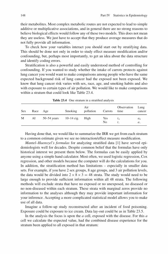
148 Part IV Statistics in Epidemiology
their metabolites. Most complex metabolic routes are not expected to lead to simpleadditive or multiplicative associations, and in general there are no strong reasons tobelieve biological effects would follow any of these two models. This does not meanthey are useless. We just have to accept that they produce average measures that donot fully provide all information.
To check how your variables interact you should start out by stratifying data.This should be done not only in order to study effect measure modification and/orconfounding, but, perhaps most importantly, to get an idea about the data structureand identify coding errors.
Stratification is also a powerful and easily understood method of controlling forconfounding. If you wanted to study whether the intake of carrots protects againstlung cancer you would want to make comparisons among people who have the sameexpected background risk of lung cancer had the exposed not been exposed. Weknow that lung cancer risk varies with sex, race, age, and smoking habits and alsowith exposure to certain types of air pollution. We would like to make comparisonswithin a stratum that could look like Table 23.4.
Table 23.4 One stratum in a stratified analysis
Sex Race Age SmokingAirpollution Carrots
Observationtime
Lungcancer
M AI 50–54 years 10–14 cig. High YesNo
t+t–
a+a–
Having done that, we would like to summarize the IRR we get from each stratumto a common estimate given we see no interaction/effect measure modification.
Mantel–Haenszel’s formulas for analyzing stratified data [1] have served epi-demiologists well for decades. Despite common belief that the formulas have onlyhistorical interest we present them below. The formulas can be easily applied byanyone using a simple hand calculator. Most often, we used logistic regression, Coxregression, and other models because the computer will do the calculations for you.In addition, the stratification method has limitations – especially in smaller datasets. For example, if you have 2 sex groups, 8 age groups, and 3 air pollution levels,the data would be divided into 2 × 8 × 3 = 48 strata. The study would need to belarge enough to provide sufficient information within all 48 strata. The followingmethods will exclude strata that have no exposed or no unexposed, no diseased orno non-diseased within each stratum. These strata with marginal zeros provide noinformation to the analyses although they may provide important information foryour inference. Accepting a more complicated statistical model allows you to makeuse of all data.
Imagine a follow-up study reconstructed after an incident of food poisoning.Exposure could be exposure to ice cream. Data lay-out could be as in Table 23.5.
In the analysis the focus is upon the a cell, exposed with the disease. For this acell we calculate the expected value, had the combined disease experience for thestratum been applied to all exposed in that stratum:

Multiplicative Model 149
Table 23.5 Stratifiedanalyses for Mantel–Haenszelanalysis
Stratum Exposure D D n
j +–
ajcjDj
bjdj
Dj
nj+nj–nj
E(aj) = Djnj+nj
Then we calculate the variance of the a cell and our estimate of the relative risk,RRMH:
Var(aj) = nj + nj − DjDj
n2j (nj − 1)
We then combine results from all strata to get a combined estimate of RR:
RRMH =∑
ajnj−nj
∑cj
nj+nj
and the χ2 test of the difference between the disease risk among exposed versusnon-exposed is (now summarized over all strata)
χ2 = (∑
aj − ∑E(aj))2
∑Var(aj)
In a study on incidence rates the table will look like Table 23.6.
Table 23.6 Stratifiedanalysis of rate data Stratum Exposure D Person-time
j +–
ajcjDj
tj+tjTj
The expected value of the a j cell becomes
E(aj) = Djtj+Tj
The variance of the a cell is
Var(aj) = Djtj+tj−
T2j

150 Part IV Statistics in Epidemiology
IRRMH =∑ ajtj−
Tj∑ cjtj+
Tj
and the χ2 test of the null hypothesis of no association between the exposure andthe disease is, like before,
χ2 =(∑
aj − ∑E(aj)
)2
∑Var(aj)
Reference
1. Mantel N, Haenszel W. Statistical aspects of the analysis of data from retrospective studies ofdisease. J Natl Cancer Inst 1959;22:719–748.

Chapter 24P Values
In the past, much emphasis was put on the so-called significance testing. The investi-gator assumed a null hypothesis stating no association between the exposure and thedisease (usually the real hypothesis would be the opposite of the null hypothesis).Then he/she would calculate a P value. The P value would indicate the probabilityof getting the data he/she found or data that were even further away from the nullhypothesis (the no-effect value), given the null hypothesis was true (and other con-ditions). If this P value was below a given level (often <0.05) it was said that thefinding was statistically significant and the null hypothesis was rejected as a likelyexplanation of the data.
There are several reasons why this practice should be abandoned. First, the inter-pretation requires a randomized trial. For a non-randomized study we would haveto add a sentence like “If this study was randomized, then. . ..” Clearly this poses asevere limitation on the P value interpretation in non-randomized studies to a levelwhere it is almost meaningless.
Second, most decisions should not be forced to follow a simple decision ruleunless it is absolutely necessary, and classifying results as significant or not sig-nificant lends itself to such a simple decision process. Significance testing wasdeveloped as a decision tool in mass production where it may serve a quality controlpurpose well. In public health we would almost never base a decision on a simplestatistical rule, and only rarely will this be the case in the decision process followinga randomized trial, although it may be so if the randomized trial is the only evidencewe have.
We have the four outcomes of a decision based upon a P value testing a nullhypothesis (H0) in Table 24.1.
Table 24.1 Type 1 and type2 errors H0 H0 accepted H0 rejected
True OK Type 1 errorFalse Type 2 error OK
As seen, two of the four outcomes are wrong. The risk of a type 1 error is set bythe significance level (often 0.05). The risk of accepting a false H0, that the effect
151J. Olsen et al., An Introduction to Epidemiology for Health Professionals,Springer Series on Epidemiology and Health 1, DOI 10.1007/978-1-4419-1497-2_24,C© Springer Science+Business Media, LLC 2010

152 24 P Values
of the exposure is overlooked, is a function of several conditions. The type 2 erroris high if the study is small or if the effect is small. It depends on the significancelevel of testing and the sample size. The power of the study equals (1 – risk of type2 error). The power indicates the probability of finding a true effect of a given sizeand with a given sample size.
It is difficult to see why we should accept to base our decision on a P level onlyand few would probably do so. P values are still computed, but more attention isgiven to estimates of association and their confidence limits, although confidencelimits often indicate only part of the uncertainty related to the measure of effect.Uncertainty is also related to residual confounding and other types of bias. Opinionsare based on the combined available evidence. Good studies carry more weight thanpoor studies. Simple replication studies carry less weight than studies that bringthe hypothesis to a more critical test. When to take action furthermore depends onthe consequences of doing nothing versus doing something. There is no P valuesubstitute for common sense and critical thinking but brain surgery may be neededto remove P values from epidemiologic papers. The most serious flaw in using Pvalues is to infer that there is no association if the P value is 0.05 or higher. Absenceof evidence is not evidence for absence of an effect! A failure to recognize thissimple fact has caused much harm to many innocent people.
Further, uncertainty is related to residual confounding and/or various types ofbias. Opinions are based upon the combined evidence available. Good studies havemore weight than poor studies. Simple replication studies carry less weight thanstudies that put the hypothesis to a more critical test. When to take action further-more depends upon the consequences of doing nothing versus doing something.There is no substitute for common sense and critical thinking.
The multiple comparison problem is a problem related to presenting only statis-tically significant results to the reader. If you generate a data source at random witha large number of exposures and a disease, then test the associations between thedisease and this exposure and then calculate P values. These P values will fall on a45◦ line as illustrated in Fig. 24.1.
The number of significant associations (that all are generated by randomness inthis example) is determined by the number of tests we perform, and since theseassociations are spurious they tend not to be replicable in other studies. We wouldlike to avoid presenting these associations, but unfortunately, there is no simple way
P value 1.0
0.05ordered association
Fig. 24.1 P value plot ofordered associations

P Values 153
of doing this. Simple correction factors, like the Bonferroni correction that approx-imately reduces your significance level by the number of tests you perform (if youdo 10 tests your level of significance should not be 0.05 but 0.005), aims at keep-ing the risk of producing one or more spurious significant results less than 0.05.Unfortunately, it is seldom that simple. First of all, this is not how serious epidemi-ologists analyze and report results. Second, the simple Bonferroni correction is oftenwrong. The principles for analyzing data are to follow a specific a priori hypothe-sis and then evaluate if your data supported the hypothesis or not. You would like toknow how much you have to adjust your prior belief in the hypothesis you had giventhe data. Furthermore, when you identify an association you should try to see howrobust it is. In your analyses you will try to see if you can make the association goaway by adjusting for confounding or other sources of error. You will check if theassociation is consistent in relevant strata, etc. You will of course also report non-significant associations in your paper. Proper analyses of epidemiologic data havenothing to do with uncritical testing for a large number of associations and onlyreporting significant P values. Remember that any source of information will onlymodify your prior belief in the association, to make this belief stronger or weaker.

Chapter 25Calculating Confidence Intervals
Confidence intervals provide more information than a P value and do not in the sameway tempt readers to make simplified conclusions; ideally they provide a range ofeffect measures that are “acceptable” given the data. If the null value (RR, IRR = 1;RD, IRD = 0) is not among these, the result is statistically significant, and theno-effect hypothesis is not a likely explanation for the data. Many would find thatthis description is too vague, but a more precise description would have to takeinto consideration a number of assumptions that are beyond this text. To calculateconfidence limits for the risk ratio or the relative risk (RR) we need to calculate thevariance of the log of the Mantel–Haenszel estimated relative risk.
The formula for the variance of the RRs is
Var( ln (RRMH)) =
∑ Djnj+nj−(n2
j − ajcj)/nj∑ ajnj−
nj
∑ cjnj+nj
The 95% confidence limits (indicated by RRL and RRUL) will be
RRLL = eln (RRMH)−1.96√
Var( ln (RRMH))
RRUL = eln (RRMH)+1.96√
Var( ln (RRMH))
The value 1.96 provides a P value of 0.05 in a standard normal distribution of√X2 values and we take the square root of the variance to get standard deviation.The variance formula for the Mantel–Haenszel odds ratio (ORMH) is
Var( ln (ORMH)) =∑
AjXi
2(∑
Ai)2
+∑
(AiYi + BiXi)
2(∑
Ai∑
Bi) +
∑BiYi
2(∑
Bi)2
where Aj = (ajdj/nj), Xj = (aj+dj)/nj, Bj = (cjbj/nj), and Yj = (cj+bj)/nj.And the two confidence limits are (like before)
155J. Olsen et al., An Introduction to Epidemiology for Health Professionals,Springer Series on Epidemiology and Health 1, DOI 10.1007/978-1-4419-1497-2_25,C© Springer Science+Business Media, LLC 2010

156 25 Calculating Confidence Intervals
ORLL = eln (ORMH)−1.96√
Var( ln (ORMH))
ORUL = eln (ORMH)+1.96√
Var( ln (ORMH))
For the Mantel–Haenszel incidence rate ratio we get
Var( ln (IRRMH)) =
∑(
Djtj + tj−T2
j
)
(∑ ajtj−
Tj
)(∑ cjtj+
Tj
)
and the two confidence limits are (like before)
IRRLL = eln (IRRMH)−1.96√
Var( ln (IRRMH))
IRRUL = eln (IRRMH)+1.96√
Var( ln (IRRMH))
Although most confidence intervals in epidemiology have no precise meaningthey are still useful as a familiar measure of part of the uncertainty inherent in ourmeasures of association. They at least remind us that other effect estimates are alsoacceptable explanations of the data.

Epilogue
The laws of nature are to be discovered, not to be invented, as Pierre LouisMaupertuis stated in the nineteenth century. These laws of nature deal with the manydifferent factors that impact our health. The laws are often complex and involvemany different component causes, and they will only reveal themselves when youcombine data from many people. For that reason epidemiology is a populationscience.
As explained in this book, population studies (epidemiologic studies) are saddledwith problems and limitations, and do not think that all the examples provided in thisbook can be generalized to all other situations. Still, epidemiologic studies are, andwill remain, the most important studies if your goals are to prevent disease, improvehealth, and provide the best possible health care.
History has shown that epidemiology, with all its problems and shortcomings, hasprovided much useful information that has improved our life expectancy and qualityof life [1]. It is therefore necessary for health professionals to at least have someknowledge about the methods epidemiologists use and their limitations. Carefullydone epidemiologic studies will not only provide new and valid information but willalso identify false beliefs and misconceptions. Nothing more than common sense isperhaps needed to do epidemiologic research, but common sense is a remarkablyrare trait that needs to be stimulated by training and education. If this book makesyou aware of what you do not know you are on your way to becoming a betterepidemiologist.
Reference
1. Holland WW, Olsen J, Florey CDV. The Development of Modern Epidemiology. OxfordUniversity Press, Oxford, 2007.
157J. Olsen et al., An Introduction to Epidemiology for Health Professionals,Springer Series on Epidemiology and Health 1, DOI 10.1007/978-1-4419-1497-2,C© Springer Science+Business Media, LLC 2010


Index
AAccording to protocol, 82Additive model, 145–146Adoption studies, 89, 91Age-specific mortality rates, 12, 19–20Alleles, 37, 93–94, 132Anti-TNF medications, 142Apolipoprotein E (ApoE) gene, 41Association, 15–17Attack rates, 30Attributable fraction, 30–32, 123
BBerkson bias, 131–132B. Hill’s criteria, 124Bias, 6, 32, 35, 39, 51, 54–56, 77, 79, 82–83,
85, 98, 103–105, 113–117, 119–125, 129,131–132, 136, 139–140, 142, 152
Blinding, 38, 81, 98, 117
CCancer of the cervix, 45, 123–124Candidate gene approach, 93Case–control study with density sampling,
69–70Case-crossover study, 85–87, 91Case–non-case study, 71–72Causal fields, 25–26, 38, 125Causal inference, 123–127Causation, 23–26, 37, 87, 125, 132, 134Censored, 7–8, 11, 16, 70–71, 73Cholecystectomy, 98, 139–140Chromosomes, 37Cohort, 6–7, 9, 12, 16, 31, 45, 55–56, 59–60,
62–65, 67–70, 73, 75–76, 78, 82, 92,97–98, 116–117, 120, 122, 135–136, 140
Cohort study, 55–56, 59–60, 65, 67–68, 76,78, 98
Colorectal cancer, 96, 140
Community diagnosis, 29Confidence interval (CI), 7–8, 15–17, 32,
61–62, 87, 109, 129, 155–157Confounder, 34, 107, 110, 124, 146–147Confounding by indication, 81, 98, 109,
139–140Copy number variants (CNVs), 37, 94, 137Counterfactual, 19, 51–52, 87Cross-sectional studies, 79, 93, 95–96Crude, 19–20, 31, 104Cumulative incidence difference, 16
DDifferential misclassification, 81, 98, 115, 129,
139–141Directed acyclic graphs (DAGs),
33–35, 110Direct standardization, 20–21Disease odds ratio, 68, 71Dizygotic (fraternal) twins, 90DNA, 37, 93–94, 136–137Dose–response pattern, 60
EThe ecological fallacy, 52Ecologic study, 52–54Effect, 15–16, 23–24, 26, 38–39, 45, 51–52,
56, 73–74, 79, 81–82, 84, 86, 89–91, 93,103, 105, 108–111, 115, 120, 123–125,129, 132–134, 139, 145–148, 151–152,155–156
Effect measure modification, 108, 120,147–148
Equipoise, 83Etiologic fraction, 32, 123Evidence-based medicine, 43Experimental design, 51, 56–57, 85Exponential formula, 17Exposure odds ratio, 68, 71
159

160 Index
Exposures, 15External validity, 105, 120
FFalse positive findings, 135Follow-up study, 15, 51, 56, 65, 67–69, 77–78,
82–83, 109–110, 114–116, 119–121, 148
GGene–environment interaction, 92–93Genes, 23, 27, 33, 37–40, 51, 89–90, 92–93,
122, 125–126, 132, 136Genome wide association study (GWAS),
93–94Genotyping, 37–38, 136Global burden of diseases, 30Glucose-6-phosphate dehydrogenase, 92
HHalf-sib studies, 90–91Hardy–Weinberg equilibrium (HWE), 137Healthy worker effect, 105Heritability, 90–91, 135–136Historical cohort, 65
IImmortal observation time, 65Incidence density, 8Incidence rate ratio (IRR), 15–17, 54–56, 60,
63, 67–70, 77, 146–148, 155–156Indirect standardization, 20–21Induced abortion, 141Induction time, 26, 28Information bias, 35, 76, 103, 113–117Intention to treat, 82–83, 98, 121, 134Interaction, 38, 92–93, 95, 145, 147–148Internal validity, 105, 120INUS principles, 25
JJuvenile diabetes, 46–47
LLatency time, 9, 26–28, 64–65, 78, 85Life expectancy, 5, 10–13, 20, 74–75, 157Linus Pauling, 40Loss to follow-up, 6–7, 15, 67–68, 120–121
MMantel–Haenszel, 148–149, 155–156Matching, 110, 136Mendelian randomization, 132–134Mendel’s laws, 37–38, 132Misclassification bias, 113
Monogenic diseases, 38–39Monozygotic (identical) twins, 90Mortality, 3–4, 11–13, 19–21, 29, 40, 43, 45,
52, 65, 75, 85, 92–93, 96, 105, 109Multiple comparison, 93–94, 135, 152Multiple testing, 135–136Multiplicative models, 146–150
NNature–nurture, 89, 91Non-differential misclassification, 115Nucleotides, 37Null hypothesis (H0), 121, 123, 150–151
OObservation time, 7, 9, 16, 20, 55–56, 62–65,
67–70, 148
PPatient controls, 72–73Perforated appendix, 97Pernicious anaemia, 95Phenotyping, 38Phenylketonuria (PKU), 25, 40, 94Placebo, 81Population at risk, 6–7, 11–12, 16, 62, 70, 72Populations, 4–5, 7, 15, 19–21, 25, 43–44, 52,
70, 85, 94, 96, 105, 125, 136Population stratification, 136Prenatal, 24, 40Prevalence, 3–6, 10, 15, 29, 41, 53, 73, 75, 77,
79, 83, 92, 111, 114, 119, 121, 125, 134Prevalence proportion, 6, 10, 15, 75, 77,
83, 114Prostate-specific antigen (PSA), 43P value, 94, 151–153, 155
RRandomization, 56, 81–82, 98, 109–110,
120–121, 132–134Randomized clinical trial (RCT), 43, 95–96,
98–99, 142Randomized trial, 43, 52, 56, 81–83, 85, 96,
98, 109–110, 119–121, 123, 132, 134, 151The rare disease assumption, 71Regression towards the mean, 129–130Relative risk, 15, 32, 59–60, 68–69, 75, 77,
86–87, 111, 116, 141, 147, 149, 155Reverse causation, 87, 132, 134Risk, 3, 5–8, 11–12Risk difference, 16, 60–61, 115Risk factors, 5–6, 29, 41, 44, 57, 63, 79, 85,
122Risk indicators, 123Robert Guthrie, 40

Index 161
SScreening, 6, 28, 40–41, 43, 45, 52, 74, 96, 122Secondary data, 30, 85Secondary identification of the source
population, 74Selection bias, 6, 54–55, 77, 82, 98, 103, 105,
119–122, 129, 139, 142Sensitivity, 113–116, 129Significance testing, 123, 151Simpson’s paradox, 108Single nucleotide polymorphisms (SNPs), 37,
94, 135, 137Specificity, 113–116, 125Stratified analyses, 63, 149
Stratum, 63, 147–149Sudden infant death syndrome (SIDS), 44, 47Sufficient cause, 25, 27Sufficient statistic, 21Survey, 29, 53–54, 75, 79, 104, 119, 121
TTwin study, 87, 90Type 1 error, 93–94, 151Type 2 error, 151–152
VVasectomy, 140–141