SpringbackR.H. Wagoner, J.F. Wang, and M. Li, The Ohio State University

This article is intended as an introductionto the concepts of springback simulation as wellas recommendations for its practice in a metalforming setting. Most of the developments focuson thin beams or sheets, where springback ismost pronounced. The underlying mechanicsof large-strain, elastic-plastic deformation aretreated in a simplified, intuitive way, withnumerous references provided for those wishingto delve into the theoretical underpinnings inmore detail. Simple bending is first considered,along with a discussion of approximations, thenbending with tension and finally, more complexnumerical treatments. Compensation of die de-sign to account for springback is also presentedbriefly.

This treatment is intended for practitionerswith widely differing backgrounds and needs.The early treatments are suited to a limited classof problems but are best suited for understandingthe direction of the effects of various materialproperties and process parameters. The roles andeffects of various simplifying assumptions arealso treated naturally with these closed-formsolutions. The later treatments are intended toaugment the practice of applied sheet forming

analysis (almost always finite element based) toinclude postforming springback analysis. As isshown, the choices of numerical parameters canbe quite different for springback, so these aspectsare emphasized.

As used throughout this article, springbackrefers to the elastically driven change of shapethat occurs after deforming a body and thenreleasing it. The concept is understood by anyonewho has manually bent a metal wire or strip. Fora sufficiently small bend radius, some part of thebending remains after unloading and some partis recovered during unloading (or has sprungback). For bend radii larger than some criticalvalue, the initial shape of the body is recovered.The recovered portion of the deformation isreferred to as springback. As such, the definitioninherently refers to a difference in geometrybetween the loaded state and the unloaded state.

The word springback as a single, unhyphen-ated word appears in virtually no standarddictionaries but has been in technical use sinceat least the early 1940s. A search of the inter-net in April 2005 found more than 26,800occurrences of the word, and a contemporaneoussearch of the ISI Web of Science (Thomson

Scientific) of published technical papers located334 such references appearing since 1980. Thesenumbers represent increases of 460 and 27%,respectively, over similar searches performed20 months earlier, in April 2003. Two inferencesmay be drawn: the technical meaning of spring-back is well established, although formal defi-nitions appearing in dictionaries lag, and interestin springback is growing rapidly.

The definition of springback can be broad,applying to the action of springs, for example,but the principal technical intent of the wordand interest in the phenomenon refers to the un-desirable shape change that occurs after forminga part. The change is undesirable because itcreates a difference of part shape from the toolshapes that were used to carry out the formingoperation. If this difference is not predictedaccurately and compensated for in the design ofthe tools, the part may not meet specifications.

Consideration of springback is of primeinterest for bodies that have high aspect ratios;that is, at least one dimension is much largerthan, or smaller than, the other dimensions.Examples include slender beams and thin sheets(Fig. 1, 2). For these cases, the overall geometric

(a) (b)

Unloaded

Formed, with tools

Initial blank

(c)

Fig. 1 Typical automotive sheet-formed part, the S-rail. (a) Formed part. (b) Finite element representation, as formed. (c) Cross-sectional schematics at three forming stages.Source: Ref 1

Name ///sr-nova/Dclabs_wip/ASM/5120_12R_01-23.pdf/A0005131/ 27/2/2006 5:27PM Plate # 0 pg 1

changes caused by springback can be very sig-nificant even though the elastic strains drivingthe springback can be tiny.

To introduce an applied example, Fig. 1(a)shows a representative automotive formed partreferred to as the S-rail (Ref 1). Figure 1(b)depicts a corresponding finite element mesh, andFig. 1(c) focuses on a schematic cross section ofthis part at three stages: initial (flat), as-formed(with tools in place), and unloaded (after spring-back). Inspection of the operation (and ignoringslight stretching at the top web of the part)reveals that the upper corners of the cross sectionare essentially bent to conform to the punchradius (the punch in this orientation lies belowthe sheet). When the tooling is removed, theseradii open up to larger radii. This is typical of anidealized bending-with-tension operation. Thesidewall regions of the formed rail or channelare drawn over the die radii (the die lies above thesheet in this orientation) over large distances,such that each element undergoes bending andunbending sequentially, also under the actionof tension. When loaded, the sidewalls are flat.The final shape of the sidewalls incorporateswhat is known as sidewall curl. The level oftension for each location is related to the binderforce, the friction with the tooling, and the workrequired to bend, unbend, and draw. If a drawbead were involved, this would add yet anotherelement to the sheet tension determination.

The primary focus in this article is on sheetmetal forming operations, such as the one shownin Fig. 1. This focus allows conclusions to bedrawn with reference to a relatively narrow rangeof thicknesses and bend radii, both of whichare small relative to the width of the body. Theequations and results are nonetheless applicableto other geometries, with restrictions specifiedas necessary.

This article is organized in sections. Thesubject of springback is first addressed for thesimplest, most easily understood cases, that is,pure bending of slender beams or sheets. Whilesuch treatments are applicable to few problemsof applied interest, their study reveals the prin-ciples governing the problem and addresses thelimitations of the various assumptions. To thesetreatments is then added the effect of super-imposed tension, which is shown to be a criticalvariable for accurate prediction of springback.From these generally closed-form treatments, aleap is made to the much more general andpractical prediction of springback for real form-ing operations, using either experience or finiteelement modeling. Finally, the design of dies andtooling using an assumed springback predictioncapability is addressed.

Pure Bending—Classical Results

In order to understand the phenomenon ofspringback, it is instructive to begin with thesimplest case and the most restrictive assump-tions. In this section, the case of pure, or simple,bending is considered, that is, bending under

the action of an applied moment without ap-plied sheet tension. The springback consists ofassumed elastic unbending on removal of theapplied moment.

Assumptions. The assumptions that apply tothis case in the simplest treatment may be listedas:

1. Plane sections remain planar.2. No change in sheet thickness3. Two-dimensional geometry, either plane

strain or plane stress in width direction4. Constant curvature (i.e., no instability of

shape)5. No stress in the radial, or through-

thickness, direction6. The neutral (stress-free) axis is the center

fiber and is the zero-extension fiber.7. No distinction between engineering and true

strain8. Isotropic, homogeneous material behavior9. Elastic straining only during springback

The validity of these assumptions is discussedin the next section, but the simple results forspringback under these conditions are firstpresented here.

Within these assumptions, the primarydifferences among treatments appearing in theliterature relate to the assumed material con-stitutive behavior. There are two basic choicesto be made: whether to treat the problem aspurely plastic or elastic-plastic, and what form ofstress-strain law to adopt in the plastic range.Results have been presented for nearly allchoices: perfectly plastic (no hardening), linearhardening (Ref 2), power-law hardening (Ref3–7), or a general approach (requiring graphicalor other numerical integration) (Ref 8, 9).

Basic Equations and Approach. The ap-proach is illustrated in Fig. 2. An initially flatsheet or beam is envisioned. For these purposes,a sheet denotes a part that is very wide relativeto its thickness and bend radius and impliesthat the deformation is nearly plane strain; thatis, the strain in width direction is zero. A beamdenotes a part that is very narrow relative tothickness and bend radius and implies thatthe deformation is nearly plane stress; that is, thestress in the width direction is zero. The part isbent to a starting radius (R) under the action of amoment (M). The value of M acting on the sheetor beam is obtained by integrating the stressdistribution as:

M=ðt=2

7t=2

sx(ex)zw(z)dz (Eq 1)

where ex is the circumferential strain, sx thecircumferential stress (Fig. 2b), t is the sheetthickness, and w(z) is the width of the sheet,which in general may vary with the z-coordinate(that is, the cross section need not be rectan-gular). Assuming a rectangular cross section,taking advantage of the symmetry of the problem(assumptions 6 and 8 in the section “Approx-imations in Classical Bending Theory” in thisarticle), and substituting into Eq 1 obtains themoment per unit width (M/w), which may beexpressed more simply:

M

w=

ðt=2

7t=2

sx(ex)z dz=2

ðt=2

0

sx(ex)z dz (Eq 2)

The strain shown in Eq 1 and 2, ex, depends on z.Within the given assumptions, the circumfer-

Pure bendingz

xy

R

r

M M

Unloaded

(a)

Flat sheet or beam

Unloaded

Stress

Loaded

z

(b)

+ t2

– t2

Fig. 2 Schematics of pure bending. (a) Configurations with coordinates defined. (b) Through-thickness stressdistribution

2 / Process Design for Sheet Forming

Name ///sr-nova/Dclabs_wip/ASM/5120_12R_01-23.pdf/A0005131/ 27/2/2006 5:28PM Plate # 0 pg 2

ential strains (ex) are linearly related to thedistance from the center of the sheet (z) andinversely to the bend radius (of the center fiberof the body) R:

ex � ex=z

R(Eq 3)

where it is assumed that the true strain (ex) andthe engineering strain (ex) are small enough to beused indistinguishably. As is shown explicitly,the bending moment can be calculated using Eq 2and 3, along with a constitutive relationshipbetween stress and strain.

Note: In order to simplify the notation, thesubscript x is dropped from the terms sx andex, with the understanding that these representthe principal components of stress and strainnormal to the beam or sheet cross section (aslabeled in Fig. 2).

In order to compute the springback afterbending, the moment per unit width of sheet,M/w, is removed from the sheet or beam whilethe material responds elastically. Because elasticstresses and strains can be superimposed, analternative view of this operation is obtainedby applying a moment (M) to the stress-free bodyin the configuration of the bent beam or sheet.An isotropic linear elastic beam or sheet has aconstitutive response of sx=E 0ex, where E 0 isthe effective modulus for the beam (plane-stresscase) or E 0=E/(1�n2), where n is Poisson’sratio, for the sheet (plane-strain case).

For elastic recovery from an initially curvedconfiguration (radius=R) to a final configura-tion (radius= r), the relationship for a body ofgeneral cross section is:

1

R7

1

r=

M

E0I(Eq 4)

where I is the moment of inertia of the crosssection.

Note: The springback results for plane strainand plane stress do not differ greatly for mostmaterials. Assuming that the bending moment isproportional to the operative flow stress for anisotropic, nonhardening, von Mises material, theplane-strain bending moment is 2=

ffiffiffi3p

(1.15)times the plane-stress moment. Assuming atypical Poisson’s ratio of 1/3, the plane-strainelastic modulus is 1.12 times the plane-stress(i.e., uniaxial tension) one. Thus, the differencesbetween Eq 4 interpreted for plane stress or planestrain is only approximately 1.15 versus 1.12, orapproximately a 3% differential. Elastic andplastic anisotropy may change this value.

Moments of inertia may be readily calculatedfor complex shapes by integration and have beentabulated for a variety of standard structuralshapes (Ref 10). For the case of a rectangularcross section, which is assumed in the remainderof this article, the moment of inertia is taken as:

I=wt3

12(Eq 5)

where t is the sheet thickness. Equation 4 maybe rewritten for a rectangular cross section in a

per-width format as:

1

R7

1

r=

M

E 0I=

12M=w

E 0t3(Eq 6)

which may be readily rewritten in the alternateform:

r

R= 17R

M

E 0I

� �71

= 17R12M=w

E 0t3

� �71

(Eq 7)

The form 1R7 1

r

� �is called springback in this

article, while the second form, r/R, is calledthe springback ratio. In general, the springbackis positive (r4R), and the springback ratiois thus greater than unity. The relationshipbetween the two measures is as Springbackratio=1/(1�R �Springback). For most applica-tions, springback as defined previously is thequantity of interest. For small curvature changes,the shape change displacements are proportionalto springback. The springback ratio is occa-sionally used with some analytical procedures,so a few results in this article are presentedusing it.

Note that a fractional error associated withthe evaluation of springback may be quitedifferent from the fractional error associatedwith the springback ratio, depending on howlarge the second term of Eq 7 is relative to 1. Thatis, when the second term is small, errors of R/rwill appear to be small even though the fractionalerrors on moment can be significant.

Equations 6 and 7 represent the fundamentalspringback result for pure bending with theassumptions listed. To apply Eq 6, it is necessaryto first choose the plane-stress or plane-strainapproximation based on width with respect tobend radius and thickness. The bending momentis computed using Eq 2 and 3 and an explicitmaterial stress-strain law (and known stressstate). This approach is used to reproduce someclassical springback results in the remainder ofthis section.

Rigid, Perfectly Plastic Result. The simplestspringback result for pure bending makes use ofa rigid (i.e., no elastic strains), perfectly plastic(no strain hardening) material model (Ref 4–6, 8,11–13). Under these assumptions, the bendingmoment (and thus the springback) is independentof the original bend radius:

M

w=2

ðt=2

0

s 00z dz=s 00 t2

4(rigid, perfectly plastic)

(Eq 8)

where s00 is the yield stress (also the flow stress)

of the material in plane stress or plane strain. Thespringback, defined here, is obtained using Eq 4:

1

R7

1

r=

3s 00E 0 t

or, alternatively,

R

r=17

3s 00 R

E 0t(rigid, perfectly plastic)

(Eq 9)

This result is often sufficient for springbackprediction, and it reveals the importance of the

principal material properties as they affectspringback:

� Springback is proportional to strength/stiffness, that is, s0/E.

� Springback is inversely proportional to sheetthickness.

More detailed analysis alters the exactform of these dependencies, but the conclusionremains the same: materials that are strong rela-tive to their elastic modulus are more susceptibleto large springback, as are thinner materials.Thus, aluminum sheet of comparable strength toa steel alloy exhibits springback approximatelythree times greater, because its elastic modulus isapproximately 1/3 as large as that of steel.

Elastic, Perfectly Plastic Result. The firstrefinement of Eq 9 is by the inclusion of elastic,perfectly plastic bending behavior (Ref 14, 15).That is, there will be an elastic core near theneutral axis. The location of the elastic-plastictransition has a z-coordinate of z*, which is foundby setting the yield strain (s0

0/E 0) equal to thebending strain (z/R):

z*=

Rs 00E 0

forRs 00E 0

jt

2

(elastic-plastic case) (Eq 10a)

t

2for

Rs 00E 0

4t

2

(elastic only, no springback)

8>>>>>>><>>>>>>>:

(Eq 10b)

Note that the extent of the elastic core isproportional to the bend radius (i.e., inverselyproportional to curvature), proportional to theyield stress, and inversely proportional tothe elastic modulus. Thus, inclusion of the elasticpart of the material response becomes pro-gressively more important for gentle bending ofhigh-specific-strength materials. As is shownlater, for typical sheet metal press forming,the bend radius is typically small enough thatthe elastic region may be neglected withoutsignificant loss of accuracy.

Evaluation of the required integral to obtainthe moment for elastic-plastic cases may beconveniently split into two terms, the secondidentical to the rigid, perfectly plastic caseoutside of the elastic core:

M

w=2

ðz*

0

E 0z

Rz dz+2

ðt=2

z*

s 00z dz

=2E 0z*3

3R+

s 00t2

47s 00z*2

(Eq 11)

Substituting the relationship for the elastic-plastic location, z* (Eq 10a), obtains the elastic-plastic moment and springback results:

M

w=

s 00t2

47

s 030 R2

3E 02(elastic, perfectly plastic)

(Eq 12)

Springback / 3

Name ///sr-nova/Dclabs_wip/ASM/5120_12R_01-23.pdf/A0005131/ 27/2/2006 5:28PM Plate # 0 pg 3

1

R7

1

r=

12M=w

E 0t3=

12

E 0t3

s 00t2

47

s 030 R2

3E 02

� �

(elastic, perfectly plastic) (Eq13)

The springback equation may be rewritten inan alternate form presented by Gardiner (Ref 14)using Eq 7:

R

r=17

3s 00 R

E 0t+

4s 030 R3

E 03t3=173x+4x3,

where x=s 00 R

E 0t(Eq 14)

Note that the left side of Eq 14 is the reciprocalof the springback ratio as defined in this article.The error introduced by ignoring the elasticcore in springback calculations may be evaluatedby comparing Eq 9 and 13 or, equivalently,Eq 8 and 11. Table 1 presents R/t ratios wherethe moment error is limited to 1, 2, 5, and 10%.For a given desired level of accuracy, the R/tratio is the largest one that can be safely con-sidered.

Typical R/t ratios for automotive press form-ing lie in the range of 5 to 25, although manyexamples outside of that range may be found,particularly with general three-dimensionalshapes that are not amenable to simple analysis.The results in Table 1 show that ignoring theelastic core leads to very small errors in thisrange for normal materials (aluminum alloyswith a yield stress of 500 MPa, or 73 ksi, areseldom suitable for complex press forming).

Rigid, Strain-Hardening Results. In addi-tion to the results presented previously, bendingmoments and springback relationships for strain-hardening material models have been pres-ented in various forms, including the followingselections:

� Empirical forms (Ref 16)� Rigid, arbitrary hardening (Ref 8)� Rigid, power-law hardening (Ref 3–7)� Rigid, linear hardening (Ref 2)

Power-law hardening models are frequentlyused for sheet forming analysis. The hardeninglaw, often attributed to Hollomon (Ref 17), maybe written as follows, in uniaxial stress and otherfixed stress- or strain-ratio forms:

s=Ken (uniaxial stress) or

s 0=K 0e 0n (general stress state) (Eq 15)

where K is the strength parameter, K 0 is the effec-tive strength parameter, n is the strain-hardeningindex, and the primes indicate that the strains andstresses to be considered must take into accountthe stress-strain state and the form of the yieldfunction (anisotropic, quadratic, etc.). (Becauseelasticity is ignored, e is the total strain, equal tothe plastic strain.) Typical results for suchhardening may be summarized as (Ref 6):

M

w=

2

n+2

� �K 0

Rn

t

2

� n+2

(Eq 16)

1

R7

1

r=

6

n+2

� �K 0

E 0t

2R

� n 1

t(Eq 17)

Elastic-Plastic Result. Bending momentsand springback relationships for elastoplastic,strain-hardening material models have also beenpresented in various forms, including:

� Elastic, power-law hardening (Ref 18, 19)� Rigid, linear hardening (Ref 18)

In order to assess the importance of strainhardening in pure bending results, moment andspringback formulas were derived based on ahardening law of the following form:

s=s0+Kenp (uniaxial stress) or

s=s 00+K 0e 0np (general case) (Eq 18)

For the plane-stress case, ep signifies theapproximate plastic strain, that is, the total strainless the elastic yield strain:

ep=e7ee �z7z*

R(Eq 19)

The second equality of Eq 19 is approximatebecause the elastic strain (ee) is treated as a con-stant corresponding to the value at first yield,rather than as evolving with hardening. Thisapproximation, adopted for simplicity, has littleeffect on the result.

The moment consists of three terms, the firsttwo identical to the elastic, perfectly plastic re-sult, that is, Eq 12 (with yield stress, s0), and thethird an integral corresponding to the additionalmoment caused by the hardening beyond theyield stress. This third term may be evaluated as:

DM

w=2

ðt=2

z*

Kenpz dz=

2K

Rn

ðt=2

z*

(z7z*)nz dz

(uniaxial) (Eq 20)

where, as before, z*=Rs0/E. Equation 20 maybe evaluated to obtain the explicit form of theincremental moment:

DM

w=

2K

Rn(n+2)

t

27z*

� n+2

+2Kz*

Rn(n+1)

t

27z*

� n+1(Eq 21)

The full moment for the elastic, hardeningplastic case is thus:

M

w=

s0t2

47

s30R2

3E2+

2K

Rn(n+2)

t

27z*

� n+2

+2Kz*

Rn(n+1)

t

27z*

� n+1

(Eq 22)

and the springback is then:

1

R7

1

r=

12M=w

Et3(Eq 23)

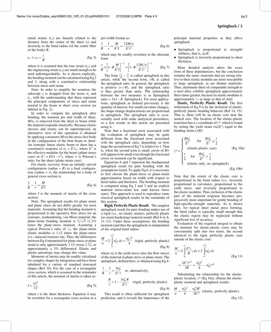
where M is given by Eq 22.Springback based on Eq 23 is compared in

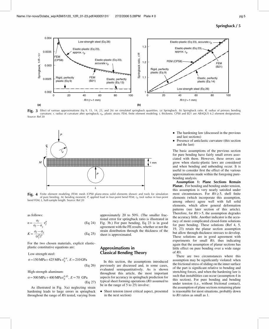
Fig. 3 with springback computed analyticallyusing elastic, perfectly plastic material behavior(Eq 13), rigid, perfectly plastic material behavior(Eq 9), and elastic-plastic finite element (FE)simulations of four-point bending (Fig. 4).(Finite element simulations are introduced laterin this article, but are included here for com-pleteness. The FE results presented in Fig. 3were verified by refining meshes and number ofintegration points until no significant changeswere observed.) The FE simulations make useof either plane-stress quadratic solid elements(labeled CPS8) or plane-stress beam elementswith shear terms (labeled B21). The elementlabels correspond to the ABAQUS (Ref 20)elements used.

For purposes of Fig. 3 and subsequent use inthis article, two material models correspondingto ratios of extremes of yield stress (sy) toYoung’s modulus for typical forming materialswere defined based on Eq 18. The soft material,low-strength steel, is based on properties appear-ing in the literature (Ref 21) for interstitial-freesteel: yield stress is 150 MPa (22 ksi), ultimatetensile strength is 310 MPa (45 ksi), and uni-form elongation is 28.5%. The hard material,high-strength aluminum, is based on the prop-erties appearing in the literature (Ref 22) for7075-T6: yield stress is 500 MPa (73 ksi), ulti-mate tensile strength is 572 MPa (83 ksi), anduniform elongation is 11%.

Parameters of Eq 18 can be determined fromthe yield stress, ultimate tensile strength, anduniform elongation by noting two conditions: 1)the engineering stress at the uniform elongationis equal to the ultimate tensile strength (sUTS),and 2) the derivative of the true stress/true plasticstrain equation is equal to the true stress at theuniform elongation (sf) (or corresponding plastictrue strain, ep

f ). Use of these two conditions, andassociating s0 of Eq 18 with the yield stress, sy,allows determination of the parameters of Eq 18

Table 1 Maximum ratios of bending radius to thickness (R/t) for specified moment errorsby neglecting the elastic core in bending (perfectly plastic)

Material

Yield stress Young’s modulus Maximum R/t for moment error of:

MPa ksi GPa 106 psi 1% 2% 5% 10%

Low-strengthsteel

150 22 210 30 85 120 190 270

Low-strengthaluminum

150 22 70 10 28 40 64 90

High-strengthsteel

500 73 210 30 26 36 57 81

High-strengthaluminum

500 73 70 10 9 12 19 27

4 / Process Design for Sheet Forming

Name ///sr-nova/Dclabs_wip/ASM/5120_12R_01-23.pdf/A0005131/ 27/2/2006 5:28PM Plate # 0 pg 4

as follows:

n=sf

sf7sy

epf (Eq 24)

K=sf7sy

(epf )

n (Eq 25)

For the two chosen materials, explicit elastic-plastic constitutive equations are:

Low-strength steel:

s=150 MPa+425 MPa e0:4p , E=210 GPa

(Eq 26)

High-strength aluminum:

s=500 MPa+400 MPa e0:45p , E=70 GPa

(Eq 27)

As illustrated in Fig. 3(a) neglecting strainhardening leads to large errors in springbackthroughout the range of R/t tested, varying from

approximately 20 to 50%. (The smaller frac-tional error for springback ratio is illustrated inFig. 3b.) For pure bending, Eq 23 is in goodagreement with the FE results, whether or not thestrain distribution through the thickness of thesheet is approximated.

Approximations inClassical Bending Theory

In this section, the assumptions introducedpreviously are discussed and, in some cases,evaluated semiquantitatively. As is shownthroughout this article, the most importantaspects for accuracy in springback prediction fortypical sheet forming operations (R/t assumed tobe in the range of 5 to 25) involve:

� Sheet tension (most critical aspect, presentedin the next section)

� The hardening law (discussed in the previousand last sections)

� Presence of anticlastic curvature (this sectionand the last)

The basic assumptions of the previous sectionfor pure bending have fairly small errors asso-ciated with them. However, these errors cangrow when elastic-plastic laws are consideredand when bending and unbending occur. It isuseful to consider first the effect of the variousapproximations made within the foregoing pure-bending analysis.

Assumption 1: Plane Sections RemainPlanar. For bending and bending under tension,this assumption is very nearly satisfied undermost circumstances. For R/ti5, shell finiteelements (which incorporate this assumption,among others) agree well with full solidelements, which allow general deformationpatterns (see later section of this article).Therefore, for R/t45, the assumption degradesthe accuracy little. Another indicator is the accu-racy of more complicated closed-form solutionsfor pure bending. These solutions (Ref 4, 5,19, 23) retain the planar section assumptionbut allow through-thickness stresses to develop.These solutions are in good agreement withexperiments for small R/t, thus indicatingagain that the assumption of planar sections haslittle effect on pure bending over a wide rangeof R/t.

There are two circumstances where thisassumption may be significantly violated: whenthe frictional stress of sliding on the inner surfaceof the part is significant relative to bending andstretching forces, and when the hardening law issuch that instabilities can occur (assumption 4 inthis section). For pure bending and bendingunder tension (i.e., without frictional contact),the assumption of plane sections remaining planeis reasonable for most situations, probably downto R/t ratios as small as 1.

0.002

0.0025

0.003

0.0035

0.004

0 20 40 60 80 100

Spr

ingb

ack,

1/R

–1/

r

R /t (t = 1 mm) R/t (t = 1 mm)

Elastic-plastic (Eq 23),accurate εp

FEM(B21)

FEM(CPS8)

Elastic-plastic (Eq 23),approx. εp

Rigid, perfectlyplastic (Eq 9)

Elastic, perfectlyplastic (Eq 13)

Low-strength steel (Eq 26)

(a)

1

1.1

1.2

1.3

0 20

(b)

40 60 80 100

Spr

ingb

ack

ratio

, r/R

Elastic-plastic (Eq 23), accurate εp

FEM(B21)

FEM (CPS8)

Elastic-plastic (Eq 23),approx. εp

Rigid, perfectlyplastic (Eq 9)

Elastic, perfectlyplastic (Eq 14)

Low-strength steel (Eq 26)

Fig. 3 Effect of various approximations (Eq 9, 13, 14, 23, and 26) on simulated springback quantities. (a) Springback. (b) Springback ratio. R, radius of primary bendingcurvature; r, radius of curvature after springback; ep, plastic strain; FEM, finite element modeling; t, thickness. CPS8 and B21 are ABAQUS 6.2 element designations.

Source: Ref 20

1 mm

rd

P

P

M

L

CL

Fig. 4 Finite element modeling (FEM) mesh (CPS8 plane-stress solid elements shown) and tools for simulationof pure bending. M, bending moment; P, applied load in four-point bend FEM; rd, tool radius in four-point

bend FEM; L, half-sample length. Source: Ref 20

Springback / 5

Name ///sr-nova/Dclabs_wip/ASM/5120_12R_01-23.pdf/A0005131/ 27/2/2006 5:28PM Plate # 0 pg 5

Assumption 2: No Change in Sheet Thick-ness. This assumption is related intimately withpure bending, for which it is very accurate,even to small R/t ratios. Thick shell results(Ref 23, 24) show this directly, although for R/tratios less than 1, some thickness changes canoccur (Ref 25). The use of the phrase “thickshell” in this article refers to a relaxation of somethin-shell approximations. This is distinct fromthe specialized use of this phrase in the mech-anics literature to refer to a particular, systematicdevelopment of the kinematics of shell theory.For bending under tension, as presented in thenext section, the thickness change is marked.

Assumption 3: Two-Dimensional Geo-metry, Either Plane Strain or Plane Stress inWidth Direction. This is not a good assump-tion for many bending operations. As illustratedin Fig. 5, as bending occurs in the principal axis,a curvature develops across the width of thespecimen. The effect is well known (Ref 26, 27).

The origin of this anticlastic curvature iseasily understood: the principal bending causeslengthening of fibers above the neutral axisand shortening of those below it. For lengthenedfibers there are Poisson contractions in the widthand thickness directions, while for the shortenedfibers there are expansions. Across the entirethickness, for pure bending, these very nearlybalance each other, hence assumption 2 (nochange in sheet thickness) is very accurate undermost circumstances.

When the width changes are considered, thetendency to develop a secondary curvature isclear. The outer fibers tend to contract laterallyand the inner ones to expand, so a concave-upcurvature is favored. For very wide geometries(relative to thickness and bend radius), the plane-strain assumption becomes the limiting case(although there will always be some anticlasticcurvature near the sheet edges). For narrowgeometries, the anticlastic curvature is un-impeded by shear terms, and the cross sectionadopts a circular shape with radius of curvatureRa=n/R (Ref 9). The plane-stress assumptionis the limiting case when there are no stressesresisting the adoption of this shape.

For pure-elastic bending, the shape of thecross section has been found analytically(Ref 28), and a literature review of the subjecthas appeared (Ref 29). In spite of the limitedaccuracy of the result for small R/t (the inaccu-racy arises by considering the bent configurationto be parabolic), the results are illuminatingfor typical sheet-forming cases.

The most important result is that the con-figuration of the bent part is determined by asingle dimensionless parameter (b) describingthe normalized width (w) of the specimen, some-times called Searle’s parameter (Ref 30, 31):

b=w2

Rt=

w

R� w

t(Searle’s parameter)

(Eq 28)

along with the Poisson’s ratio, n. The actualshape of the cross section for various valuesof b is illustrated in Fig. 6, where the bend radii

are also shown assuming a fixed width of 50and unit thickness of 1. The results in Fig. 6correspond to the analytic solution as follows,where C1 and C2 are numerical constants:

z

t

� =C1 cosh

ya

w

� cos

ya

w

�

+C2 sinhya

w

� sin

ya

w

� (Eq 29)

where C2,1=nffiffiffiffiffiffiffiffiffiffiffiffiffiffiffiffiffiffi

3 17n2ð Þp

·sinh a

2

�cos a

2

�+ cosh a

2

�sin a

2

�sinh (a)+ sin (a)

with a=ffiffiffiffiffiffiffiffiffiffiffiffiffiffiffiffiffiffi3(17n2)4

p ffiffiffib

p:

For b greater than approximately 100, theedge regions look similar and the center regionis essentially flat, thus implying that plane-strainconditions are accurate except at the local edgeregions. For small b, the cross-sectional shapeis essentially circular, which implies that thestresses resisting this curvature may be safelyignored (i.e., plane stress).

The transition from the plane-stress limit tothe plane-strain limit is a smooth function of b,as shown in Fig. 7. The limiting values of bfor specified errors of the effective moment ofinertia are shown in Table 2.

For springback application, the most impor-tant effect of anticlastic curvature is two-fold:on the bending moment-curvature relationship,and on the elastic unloading response. The latterwill depend greatly on the degree to which theanticlastic shape persists, that is, how muchof the anticlastic shape is retained after unload-ing. For the case of pure-elastic bending andunloading, there is no difference in springback,that is, zero springback, for cases with or with-out anticlastic effects. Persistent anticlasticcurvature is particularly important for the typicalsheet-forming case bending and unbending, asis discussed in the last section of this article. Forparts curved in three dimensions, the anticlasticcurvature may manifest itself as wrinkling,twisting, or generalized distortion. See,for example, the wrinkled area of the S-rail(Fig. 1a).

Assumption 4: Constant Curvature (i.e., NoInstability in Shape). This is closely relatedto assumption 1. For bending and bending undertension, instabilities can occur because of shear

z

Ra

R

x

y

Fig. 5 Anticlastic surface with two orthogonal curva-tures. R, radius of primary bending curvature;

Ra, radius of anticlastic curvature.

–0.05

0

0.05

0.1

0 0.1 0.2 0.3 0.4 0.5

Nor

mal

ized

def

lect

ion,

z/t

Normalized width coordinate, y/w

β = 2.5 (R = 1000)

β = 5 (R = 500)

β = 25 (R = 100)

β = 100 (R = 25)

β = 250 (R = 10)β = 500 (R = 5)

t = 1, w = 50ν =1

3

Fig. 6 Shape of cross sections for various values ofSearle’s parameter, b= (w2/Rt). z, thickness

coordinate; t, sheet thickness; y, width coordinate; w, sheetwidth; n, Poisson’s ratio; R, radius of primary bendingcurvature; b, Searle’s parameter

1 3

1.00

1.05

1.10

1.15

0 20 40 60 80 100

φ (=

EI/M

R)

Normalized section width, w 2/Rt

ν =

Plane-stress limit (φ=1.0)

Plane-strain limit (φ = 1.125)

Elastic bending

Fig. 7 The transition from the plane stress to planestrain, as a function of b= (w2/Rt). w, anticlastic

factor; E, Young’s modulus; I, moment of inertia; M,bending moment; R, radius of primary bending curvature;w, width; t, thickness; n, Poisson’s ratio

Table 2 Limiting values of b (w2/Rt) forspecified accuracy limits using plane-stressor plane-strain bending formulas

b limit

Limiting value of b for an accuracy limit of:

1% 2% 5% 10%

Plane stress(b5)

2 3 5 34

Plane strain(b4)

170 42 7 2

6 / Process Design for Sheet Forming

Name ///sr-nova/Dclabs_wip/ASM/5120_12R_01-23.pdf/A0005131/ 27/2/2006 5:28PM Plate # 0 pg 6

banding, for example. These instabilities areexpected to be of a similar magnitude andimportance and in the same range of strains asfor tension or compression. Therefore, when astable hardening law is obtained (without ser-rated yielding, Luder’s banding, or yield-pointphenomenon), bending may be assumed tobehave similarly.

Assumptions 5, 6, and 7: No Stress inthe Radial, or Through-Thickness, Direction.The Neutral (Stress-Free) Axis is the CenterFiber and is the Zero-Extension Fiber. NoDistinction between Engineering and TrueStrain. These three assumptions are closely re-lated and may be considered together naturally.To consider these effects profitably, it is simplerto ignore, for the moment, anticlastic curvature.Each of these assumptions is closely related tothe R/t ratio to which a flat beam or plate is bentinitially. The effect of bending to R/t less thanapproximately 5 produces significant through-thickness stresses in the interior of the body andcauses the stress-free axis to vary significantlyfrom the zero-extension fiber. Bending to smallR/t also produces large strains at the outer fibers,thus making the distinction between true andengineering strains more significant (Ref 32).

The last of these effects is the simplest toquantify. In order to do so, consider the elastic-plastic result of Eq 20, but this time evaluatethe strains in terms of true strains, that is:

ep=e7ee � ln 1+z

R

� 7ln 1+

z*

R

� �(Eq 30)

Note that again the additional elastic strain thataccrues with strain hardening after the elastic-plastic transition point has been ignored. Thisallows Eq 20 to be rewritten as:

M 0

w=2

ðt=2

z*

Kenpz dz

=2K

ðt=2

z*

ln 1+z

R

� 7 ln 1+

z*

R

� �� �n

z dz

(Eq 31)

where, except for the use of true strains, all theother assumptions remain the same. Evaluationof Eq 31 shows that the error on M introducedby neglecting true strain is 3.8% for R/t=1 andless than 0.64% for R/ti5. Therefore, otherassumptions introduce larger errors than thisone. (Note that a true kinematical descriptionof bending, whether finite or infinitesimal, isnot used for any derivations here. Only theevaluation of strain differs.)

The remaining assumptions related to smallR/t can be assessed by the thick-shell solutionsfor rigid, perfectly plastic behavior presentedfirst by Hill (Ref 33) and later in simplified forms(Ref 4, 5) and less restrictive forms for elastic-plastic cases (Ref 19). The conditions foundto hold even during bending to small R/t areplane strain (assumed) and no thickness change.

Maintaining these conditions during bending tosmall R/t requires consideration of the quadraticterms in the value of the circular arc. The resultsshow that significant through-thickness stressesdevelop and the stress-free fiber is no longerthe zero-extension fiber. The details of the deri-vations may be found in the references provided,but the general result is that the total true strainfor the more precise form is given by:

e= ln 1+t

2R

� 2

+2z

R

� �� �1=2

(Eq 32)

and the plastic problem must be solved incre-mentally in order to determine the stress dis-tribution throughout the plastic deformation.

Figure 8 illustrates the relative magnitude ofthe various approximations for pure bending.The deviations are quite small for the purebending case.

Assumption 8: Isotropic, HomogeneousMaterial Behavior. For fixed stress state(plane stress, for example) or strain state (planestrain, for example), the introduction of aniso-tropy, elastic and plastic, makes no fundamentalchange in the treatment of two-dimensionalbending and springback results. While an ex-tensive treatment of anisotropy is beyond thescope of this article, a simple result can illustratethe general procedure. For more complicatedcases, FE analysis is usually required, and FEprograms usually have capabilities incorporatingmaterial anisotropy.

It is important to note that anisotropy doesnot affect the basic equations for the simplebending case. For the plastic bending, the rela-tionship between tensile strain at a given fiberand the fiber location (Eq 3) is independent ofanisotropy. The relationship between the normalprincipal stress (sx) and the bending moment(Eq 2) is also unchanged. For the elastic un-loading, the relationship governing the changeof curvature remains the same, except that themodulus is the effective one relating tensilestrain (ex) to normal principal stress (sx), takinganisotropy into account.

The role of anisotropy may be reflected suffi-ciently in a generalized elastic relationship:

sx=E 0ex=fEEex (elastic) (Eq 33)

where E 0 is the effective modulus for the givenstrain-stress state, and fE is a constant factorequal to E 0/E.

For the plastic relationship, it should be notedthat strain hardening is usually specified in termsof effective strain (e) and stress (s) based on atensile test:

�s=f (�e) for example �s=K �en (Eq 34)

Using similar notation, the constant factorreflecting plastic anisotropy and stress-strainstate may be defined (Ref 34, 35):

�e=feex, �s=fssx (Eq 35)

For any fixed anisotropy and strain-stressstate, the values of fE, fs, and fe may be found and

used to complete the basic bending and spring-back equation, such as Eq 2 to 4.

As an example, consider a sheet with normalplastic anisotropy according to Hill’s quadraticyield function (Ref 33). The factors fe and fscan be derived for a given plastic anisotropyparameter (Ref 34), r, as:

fe=1+�rffiffiffiffiffiffiffiffiffiffiffiffi1+2�rp , fs=

ffiffiffiffiffiffiffiffiffiffiffiffi1+2�rp

1+�r(Eq 36)

The necessary strain-hardening relationship,sx(ex) in Eq 2, may then be found in terms of ameasured uniaxial hardening law, �s=f (�e):

sx(ex)=�s

fs=

1

fsf (�e)=

1

fsf (feex)=

1

fsf fe

z

R

�

(Eq 37)

The substitution may be illustrated con-veniently by taking a particular hardening law,say �s=K�en:

sx=K

fsfe

z

R

� n

=K 1+�rð Þffiffiffiffiffiffiffiffiffiffiffiffi

1+2�rp 1+�rffiffiffiffiffiffiffiffiffiffiffiffi

1+2�rp z

R

� �n

=1+�rð Þn+1

1+2�rð Þn+1

2

Kz

R

� n

=K 0z

R

� n

(Eq 38)

where K 0 represents all of the needed changes.The same procedure may be applied to any strainstate, tensile hardening law, and fixed plasticanisotropy.

It should also be noted that an assumption ofsymmetric yielding in tension and compressionhas been made. For as-received sheet material,this is usually a reasonably accurate picture ofthe stress-strain behavior. However, as is dis-cussed in the section, “Applied Analysis ofSimple Forming Operations” in this article thehardening behavior can become complex in re-verse bending, which is common in many sheet-forming situations. Under these conditions,the Bauschinger effect on strain reversal mustbe considered. (Strictly speaking, some strainincrement reversal can take place in single bend-ing, because the neutral surfaces move relativeto the midplane. This effect appears not to havebeen analyzed and is likely very small in prac-tical cases.)

40

80

120

160

0 2 4 6 8 10

Mom

ent/w

idth

, N

Ratio of bending radius to thickness, R/t

Low-strength steel (Eq 26), pure bending

Thick shell (engineering strain)

Thin shell (engineering strain)

Thick shell (true strain)

Thin shell(true strain)

Fig. 8 Comparison of various approximations forelastoplastic pure bending.

Springback / 7

Name ///sr-nova/Dclabs_wip/ASM/5120_12R_01-23.pdf/A0005131/ 27/2/2006 5:28PM Plate # 0 pg 7

Finally, initial material properties are assumedto be the same at each point in the body.

Assumption 9: Springback Occurs Elasti-cally. For all pure bending and nearly allbending under tension cases, this is very accu-rate. However, contrary to assertions in theliterature (Ref 36), elastic-plastic springbackcan occur for bending under high sheet tensions(approaching and beyond the yield stress)(Ref 37–40) and when the material behavior istime-dependent (i.e., via creep or anelasticity)(Ref 41, 42). A few examples of such situationsare mentioned in the section “Applied Analysisof Simple Forming Operations” in this article.

For most situations, these effects can beignored without greatly affecting the result.However, it should be noted that unloading itselfmay involve inelastic effects (Ref 43) that pro-duce changes in the observed modulus (Ref 44).There has been no clear approach on how sucheffects can be incorporated in springback ana-lysis except for adjusting the effective elasticmodulus.

Bending with Tension

The effect of superimposed tension duringbending plays a dominant role in determiningspringback, as is demonstrated with simpleanalyses. Nearly all sheet-forming operationsinvolve at least some sheet tension, whetherintroduced by remote sections of the partundergoing deformation, local friction con-ditions, or the intentional action of a draw beador other restraint. Increasing sheet tension toreduce springback and its variability has beenthe principal industrial solution to the problemof inadequate shape fixability.

Analyses similar to those for pure bendingcan be carried out by relaxing just one of theassumptions listed in the first section, namely thesixth one, that is, that the neutral (stress-free)axis is the center fiber and is the zero-extensionfiber. The sheet thickness may change sub-stantially if the tension is high during bending(Ref 45) (and particularly for bending andunbending, which is not considered until thenext section), but this effect is often ignoredfor simplicity. (For FE simulation, in the nextsection, shell elements usually assume zerothickness change in one time step, but the thick-ness is updated at the end of each step.)

Springback solutions for bending with tensionhave been presented with various levels of com-plexity, including elastic, perfectly plastic (Ref6–13); elastic, power-law hardening (Ref 18, 19,46–48); elastic, linear hardening (Ref 18, 49, 50);and rigid, power-law hardening (Ref 51–54).Extension to more complex cases includes:biaxially loaded plates (Ref 36), bending tosmall radii with tension (Ref 19), the effect onnonsimultaneous tension and bending (i.e., pre-bending or postbending) (Ref 51), taking intoaccount section changes in narrow strips (Ref 7),the role of nonuniform deformation (Ref 55),

results for laminated sheets (Ref 56), and theeffect on formability and residual-stress dis-tribution (Ref 57).

Elastic, Perfectly Plastic Result. Thesimplest elastic, perfectly plastic solution forbending with tension is sufficient to reveal thedominating importance of tension relative toother variables. Initially considering the thick-ness constant, the strain distribution through thesheet thickness is a simple superposition of atensile or membrane strain (em) and the bendingstrain (eb) as before:

e=em+eb=em+z

R(Eq 39)

At the neutral axis (assumed to be the zero-extension axis), located at z0, the strain is zero,so an expression relating the membrane strainand the neutral axis location is obtained:

em=7z0

R(Eq 40)

The stress distribution is similar to the oneshown in Fig. 9, which may be integrated toobtain the overall sheet tension, T, (per unitwidth, w) operating:

T

w=ðt=2

7t=2

s 00 dz=ðz0

7t=2

7s 00 dz+ðt=2

z0

s 00 dz=72z0s00

(Eq 41)

It is convenient to rewrite Eq 41 in termsof normalized quantities: z0/t, the fractionallocation of the neutral axis, and T, the averagesheet tension stress (T divided by sheet widthand thickness) divided by stress to yield the

sheet (s00), yielding T= T

wts 00

� . In terms of these

reduced variables, Eq 41 becomes:

z0

t

� =7

T

2(Eq 42)

With the location of the neutral axis knownexplicitly in terms of the sheet tension, themoment may be evaluated in closed form:

M

w=

s 00t 2

417T

2h i

, or (Eq 43)

M=w

t2

� �=

s 004

17T2

h i(Eq 44)

where Eq 44 emphasizes the proper normal-ization with thickness. The springback may thenbe presented in standard and normalized closedforms with the help of Eq 6 and 14 as:

1

R7

1

r=

12M=w

E 0t3=

3s 00E 0t

17T2

h i(Eq 45)

R

r=17

3s 00E 0

R

t

� �17T

2h i

(Eq 46)

Equations 45 and 46 ignore the thicknesschange that occurs by the action of the sheet

Hardening

Perf–plastic

Elastic core

Neutral axis

Center linez0

z1*

*

z

σ

z1,2 = z0 ±Rσ′0

E ′

z2*

− t2

+ t2

Fig. 9 Schematic of the stress distribution in a beam or sheet, bent to radius R, with definition of various coordinatesused in the analysis of springback

8 / Process Design for Sheet Forming

Name ///sr-nova/Dclabs_wip/ASM/5120_12R_01-23.pdf/A0005131/ 27/2/2006 5:28PM Plate # 0 pg 8

tension; that is, final thickness t is assumed to beequal to original thickness t0. The expressionsmay be approximately corrected for thicknesschanges by assuming that the final thickness isrelated to the original thickness such that thevolume is maintained using the membrane strain(a linear approximation for the definition ofstrain is used for simplicity); that is:

t7t0

t0=7em=

z0

R=7

tT

2R(Eq 47)

where t0 is the initial thickness, and the finalthickness, t, is given by:

t=1

t0

+T

2R

� �71

ort

R=

1

(R=t0)+T=2

(Eq 48)

which gives an expression for the final thicknessthat may be substituted into Eq 45 and 46 toobtain thickness-corrected versions:

1

R7

1

r=

12M=w

E 0t3=

3s 00E 0R

R

t0

+T

2

� �(17T

2)

(Eq 49)

R

r=17

RM=w

E 0I=17

3s 00E 0

R

t0

+T

2

� �(17T

2)

(Eq 50)

The results represented by Eq 46 and 50 areshown graphically in Fig. 10. As can be seenreadily, the application of sheet tension sub-stantially reduces springback. For the perfectlyplastic case, springback disappears when thenormalized sheet tension approaches unity, thatis, when the average tensile stress approachesthe appropriate yield stress. By setting T=0, thepure bending result (Eq 9, for example) isobtained.

Rigid, Power-Law Hardening Result. Usingthe approach followed previously, the spring-back predicted for bending with tension can bederived. Unfortunately, it is not in a form asconvenient as for the perfectly plastic case. The

only additional complexity is that t cannot befound explicitly in terms of T , so that M cannotbe written as an explicit function of T . It issimplest to proceed by choosing R/t0 and z0/t0as independent variables, then evaluating thesheet tension, bending moment, and thus spring-back. In this way, springback may be obtainedas a function of sheet tension but not in a closedequation form.

A power-law hardening law with a yield stressas in Eq 15 is adopted, and similar assumptionsto the ones mentioned previously are made.Because total strain is represented by Eq 39,the stress throughout the sheet thickness is:

s=

s 00+K 0en, e40 or

s 00+K 0z7z0

R

� n

, z4z0

7 s 00+K 0 ej jn �

, e50 or

7s 007K 0z07z

R

� n

, z5z0

8>>>>>><>>>>>>:

(Eq 51)

where, as was previously done, the plastic strainis approximated by the total strain (evaluatedusing the linear, small-strain definition) minusthe elastic strain at yield. The normalized sheettension and bending moment increment (beyondperfectly plastic) may then be obtained as:

T=72z0

t

� +

K 0

(n+1)s 00

t

R

� n

·1

27

z0

t

� �n+1

71

2+

z0

t

� �n+1" #

(Eq 52)

DM=w

t2=K

t

R

� n 0:5+ z0

t

�n+2+ 0:57 z0

t

�n+2

n+2

"

7z0

t

� 7

0:57 z0

t

�n+1+ 0:5+ z0

t

�n+1

n+1

#

(Eq 53)

where the current thickness must be evaluated interms of z0 using either the true-strain definition

or the small-strain approximation:

t

t0

= expz0

R

� � 1+

z0

R

� (Eq 54)

Equation 53 represents the additional bendingmoment caused by strain hardening that must beadded to the perfectly plastic moment (Eq 43).The springback ratio is then evaluated usingEq 7. The final springback ratio is shown inFig. 11.

Corrections to the Simple Power-LawHardening Result. It is possible to obtain moreaccurate solutions for this case; however, theequations become rather bulky, will usuallyrequire numerical evaluation of integrals, andthey will differ for each kind of hardening lawconsidered. (In the truly arbitrary case, anumerical integration can be carried out toobtain the appropriate solution.) Nonetheless, itis useful to illustrate the additional terms thatcan be considered for completeness and esti-mation of importance (still adopting assumptions1 and 3).

For large T or small R/t (i.e., large strain), thetrue-strain definition should be used such thatthe strains no longer vary linearly through thethickness, except approximately:

e=em+eb= ln 17z0

R

� + ln 1+

z

R

�

= ln 17z0

R

� 1+

z

R

�

= ln 17z0

R+

z

R7

z0z

R2

�

ffi7z0

R+

z

R17

z0

R

� (Eq 55)

Inclusion of the large strain formula via Eq 55will usually require numerical evaluation ofthe integrals to obtain T and M. Furthermore,bending to large curvatures (R/t less thanapproximately 5) introduces errors in the otherapproximations that are more significant thanthe small strain form (see the section “Approx-imations in Classical Bending Theory” in thisarticle). Forms equivalent to the last approximate

Normalized sheettension, T

0.80

1.0

1.2

1.4

1.6

1.8

0 50 100 150 200

Spr

ingb

ack

ratio

, r/R

R/t

0.80

1.0

1.2

1.4

1.6

1.8

0 50 100 150 200

Spr

ingb

ack

ratio

, r/R

R/t

0

0.2

0.4

0.6

0.8

1.0

0

0.2

0.4

0.6

0.8

1.0Elastic, perfectly plasticConstant thickness (Eq 46)

Low-strength steel

E=210 GPa

σ0=150 MPa

(a) (b)

Normalized sheettension, T

Elastic, perfectly plasticVarying thickness (Eq 50)

Low-strength steel

E =210 GPa

σ0=150 MPa

Fig. 10 Effect of sheet tension on springback for an elastic, perfectly plastic constitutive equation for low-strength steel. (a) Constant thickness. (b) Changing thickness. r, radius ofcurvature after springback; R, radius of primary bending curvature; t, sheet thickness; E, Young’s modulus; s0, initial yield stress

Springback / 9

Name ///sr-nova/Dclabs_wip/ASM/5120_12R_01-23.pdf/A0005131/ 27/2/2006 5:28PM Plate # 0 pg 9

one shown in Eq 55 have been used in the deri-vations already presented.

Figure 12 shows that the use of true or engi-neering strain (et) has little effect on eitherthe thin-shell or thick-shell solutions. Even atR/t=2, the error is a few percent, and it isinconsequential for R/ti5, where the overallapproach applies.

The proper plastic strain can be found bysubtracting the elastic strain, which dependson the current flow stress of the material:

ep=et7s 0fE 0

=et71

E 0s0+Ken

p

�

=et7s0

E 0+

Kenp

E 0

(Eq 56)

Equation 56 cannot be rewritten to find ep

explicitly, as required for substitution in thehardening law, but the result may be usednonetheless in evaluating the required integralnumerically. Note that the third term on the rightside of Eq 56 has been ignored throughoutthe previous derivations, thus enabling explicitevaluation of ep from et. This has little effectfor materials with typical hardening laws(Fig. 13).

For large R/t (small bending strain), the elasticcore may make an appreciable contribution tothe evaluation of the bending moment. (Thiswas previously illustrated for the nonhardeningcase.) In this case, the integrals for T and M arecarried out over only the part of the thicknesssubjected to plastic strain. The results for hard-ening can be added to the elastic, perfectlyplastic result (e.g., Eq 12) to obtain the fullsolution, as was illustrated in the previous sec-tion for pure bending.

The result for the plastic part of these quan-tities, say T and DM, is the same as Eq 52 and 53,with z0 replaced by z1* and z2*, where z1* and z2*

are the location of the transitions from elasticto plastic behavior above and below the

neutral axis. That is:

T=72z0

t+

K

(n+1)s0

t

R

� n

·1

27

z1*

t

� �n+1

71

2+

z2*

t

� �n+1" #

(Eq 57)DM

w=K

1

R

� �n

·(0:5t7z1*)

n+2+(0:5t+z2*)n+2

n+2

"

+z1*(0:5t7z1*)

n+17z2*(0:5t+z2*)n+1

n+1

#

(Eq 58)

M

w=

2

3E 0R2 s 00

E 0

� �3

+s 004

· t272 z1*2+z2*

2 �� � (Eq 59)

Care must be taken using Eq 57 and 58 that z0,z1*, and z2* are not assigned nonphysical valuesoutside of the sheet thickness. That is, the fol-lowing rules apply to all of the calculationsillustrated so far:

z0=

7emR 7t

2j7emRj

t

2t

27emR4

t

2

7t

27emR57

t

2

8>>>>><>>>>>:

(Eq 60)

z1*=z0+

Rs 00E 0

z0

Rs 00E 0

jt

2t

2z0+

Rs 00E 0

4t

2

8><>: (Eq 61)

z2*=z07

Rs 00E 0

z07Rs 00E 0

i7t

2

7t

2z07

Rs 00E 0

57t

2

8><>: (Eq 62)

Evaluation of Eq 58 and 59 (Table 3), showsthat for 05T51, the maximum error caused byneglecting the elastic core is 0.17% (R/t=25) insheet-forming range and grows to 4.6 and 13.8%for R/t of 100 and 200, respectively.

The foregoing results and discussions showthat for the typical sheet-forming regions (55R/t525), the elastic response of the material maybe safely ignored, along with more complicatedtreatments of the strain and thick shells. For largeR/t, the elastic strains become significant, and forsmaller R/t, the thick-shell approach and properplastic-strain measures become significant.

Applied Analysis ofSimple Forming Operations

For a typical industrial sheet-forming opera-tion, the sheet workpiece is pressed betweennearly rigid tools with draw-in constraintsenforced, usually via draw beads. The generaloperation may be arbitrary in three dimensions,and conformance to the tools is by no meansassured (Ref 58), thus making it impossible toknow, a priori, the bend radius of the sheet.Many material elements undergo bending andunbending with superimposed tension, whereasthe closed-form analyses usually assume a flatstarting configuration in both in-plane directions.Determining sheet tension, which was shownin the last section to be critically important inspringback, is complex, depending on friction,bending and unbending, and boundary con-straints. All of these variables may changethroughout the part and the forming stroke, oversmall distances and times.

For arbitrary, three-dimensional (3-D) form-ing operations, FE analysis (or a similar numer-ical method) is required throughout the formingoperation to obtain a final, as-formed state. Thisconfiguration (with tool contact forces) maythen be used as a basis for a general springback

50

60

70

80

90

0 2 4 6 8 10

Mom

ent/w

idth

, N

Ratio of bending radius to thickness, R /t

Low-strength steel (Eq 26)T = 0.5, bend under tension

Thick shell (engineering strain)

Thin shell (engineering strain)Thick shell (true strain)

Thin shell (true strain)

Fig. 12 Comparison of bending moment using thin and thick shells, with eitherengineering strain or true strain. T, normalized sheet tension

1.0

1.1

1.2

1.3

1.4

0 20 40 60 80 100

0

0.2

0.4

0.6

0.8

1.0

1.2Spr

ingb

ack

ratio

, r/R

R /t

Low-strength steel (Eq 26)

(Eq 7, 58, 59)

Normalized sheet tension, T

Fig. 11 Role of normalized sheet tension and bend radius on springback forelastoplastic, hardening behavior (Eq 58 and 59) of low-strength steel

(Eq 26). See Eq 7, 58, and 59. r, radius of curvature after springback; R, radius of primarybending curvature; t, sheet thickness

10 / Process Design for Sheet Forming

Name ///sr-nova/Dclabs_wip/ASM/5120_12R_01-23.pdf/A0005131/ 27/2/2006 5:28PM Plate # 0 pg 10

analysis using the same, or a different, FE model.Such analysis is discussed subsequently; how-ever, the application of two-dimensional (2-D)closed-form methods is possible and profitablefor some classes of forming operations that arefirst mentioned.

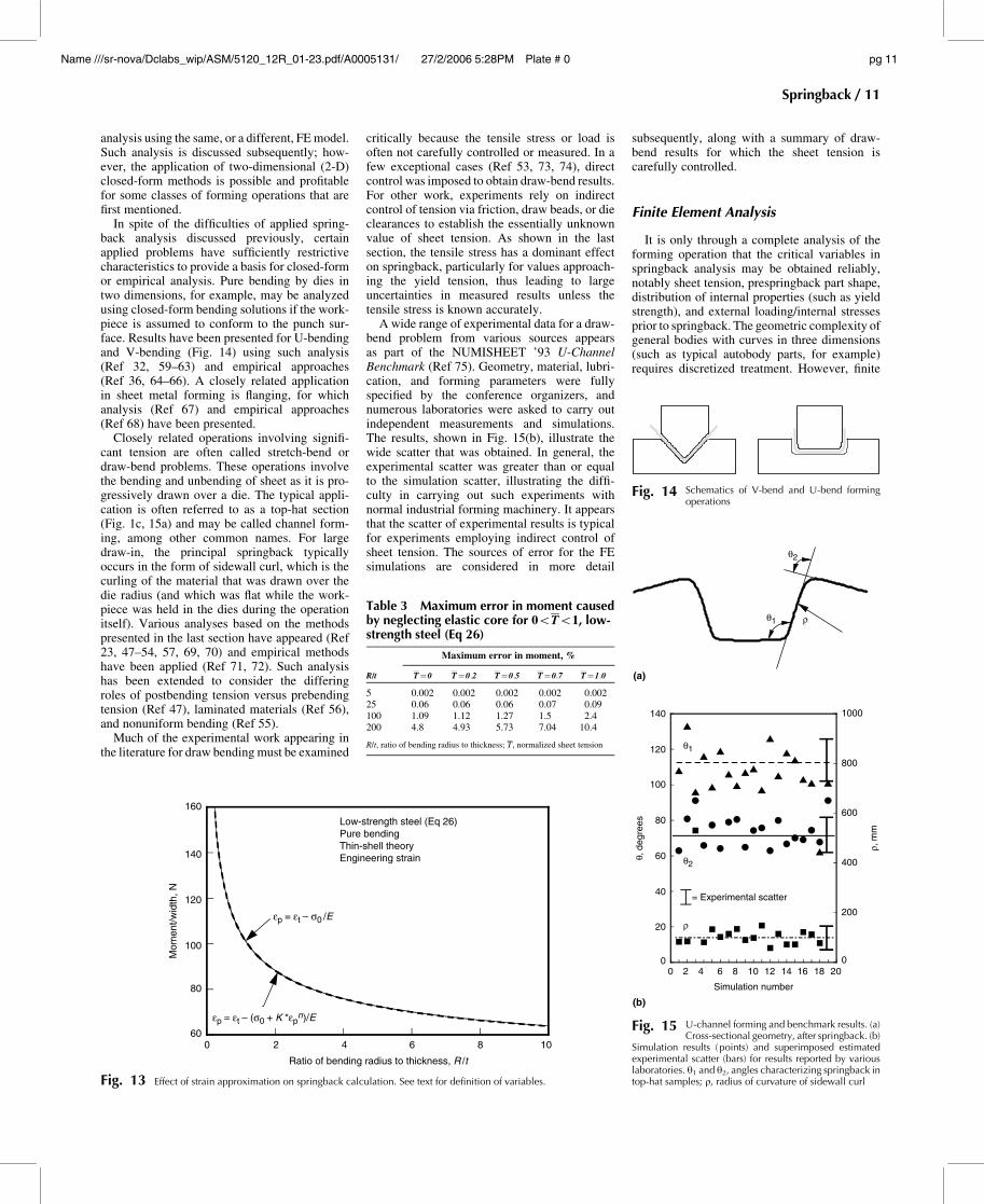
In spite of the difficulties of applied spring-back analysis discussed previously, certainapplied problems have sufficiently restrictivecharacteristics to provide a basis for closed-formor empirical analysis. Pure bending by dies intwo dimensions, for example, may be analyzedusing closed-form bending solutions if the work-piece is assumed to conform to the punch sur-face. Results have been presented for U-bendingand V-bending (Fig. 14) using such analysis(Ref 32, 59–63) and empirical approaches(Ref 36, 64–66). A closely related applicationin sheet metal forming is flanging, for whichanalysis (Ref 67) and empirical approaches(Ref 68) have been presented.

Closely related operations involving signifi-cant tension are often called stretch-bend ordraw-bend problems. These operations involvethe bending and unbending of sheet as it is pro-gressively drawn over a die. The typical appli-cation is often referred to as a top-hat section(Fig. 1c, 15a) and may be called channel form-ing, among other common names. For largedraw-in, the principal springback typicallyoccurs in the form of sidewall curl, which is thecurling of the material that was drawn over thedie radius (and which was flat while the work-piece was held in the dies during the operationitself). Various analyses based on the methodspresented in the last section have appeared (Ref23, 47–54, 57, 69, 70) and empirical methodshave been applied (Ref 71, 72). Such analysishas been extended to consider the differingroles of postbending tension versus prebendingtension (Ref 47), laminated materials (Ref 56),and nonuniform bending (Ref 55).

Much of the experimental work appearing inthe literature for draw bending must be examined

critically because the tensile stress or load isoften not carefully controlled or measured. In afew exceptional cases (Ref 53, 73, 74), directcontrol was imposed to obtain draw-bend results.For other work, experiments rely on indirectcontrol of tension via friction, draw beads, or dieclearances to establish the essentially unknownvalue of sheet tension. As shown in the lastsection, the tensile stress has a dominant effecton springback, particularly for values approach-ing the yield tension, thus leading to largeuncertainties in measured results unless thetensile stress is known accurately.

A wide range of experimental data for a draw-bend problem from various sources appearsas part of the NUMISHEET ’93 U-ChannelBenchmark (Ref 75). Geometry, material, lubri-cation, and forming parameters were fullyspecified by the conference organizers, andnumerous laboratories were asked to carry outindependent measurements and simulations.The results, shown in Fig. 15(b), illustrate thewide scatter that was obtained. In general, theexperimental scatter was greater than or equalto the simulation scatter, illustrating the diffi-culty in carrying out such experiments withnormal industrial forming machinery. It appearsthat the scatter of experimental results is typicalfor experiments employing indirect control ofsheet tension. The sources of error for the FEsimulations are considered in more detail

subsequently, along with a summary of draw-bend results for which the sheet tension iscarefully controlled.

Finite Element Analysis

It is only through a complete analysis of theforming operation that the critical variables inspringback analysis may be obtained reliably,notably sheet tension, prespringback part shape,distribution of internal properties (such as yieldstrength), and external loading/internal stressesprior to springback. The geometric complexity ofgeneral bodies with curves in three dimensions(such as typical autobody parts, for example)requires discretized treatment. However, finite

60

80

100

120

140

160

0 2 4 6 8 10

Mom

ent/w

idth

, N

εp = εt – σ0 /E

Low-strength steel (Eq 26)Pure bendingThin-shell theoryEngineering strain

εp = εt – (σ0 + K *εpn)/E

Ratio of bending radius to thickness, R /t

Fig. 13 Effect of strain approximation on springback calculation. See text for definition of variables.

Table 3 Maximum error in moment causedby neglecting elastic core for 05T51, low-strength steel (Eq 26)

Maximum error in moment, %

R/t T=0 T=0:2 T=0:5 T=0:7 T=1:0

5 0.002 0.002 0.002 0.002 0.00225 0.06 0.06 0.06 0.07 0.09100 1.09 1.12 1.27 1.5 2.4200 4.8 4.93 5.73 7.04 10.4

R/t, ratio of bending radius to thickness; T , normalized sheet tension

Fig. 14 Schematics of V-bend and U-bend formingoperations

θ1

θ2

ρ

(a)

(b)

0

20

40

60

80

100

120

140

0

200

400

600

800

1000

0 2 4 6 8 10 12 14 16 18 20

θ, d

egre

es

ρ, m

m

Simulation number

θ1

θ2

ρ

= Experimental scatter

Fig. 15 U-channel forming and benchmark results. (a)Cross-sectional geometry, after springback. (b)

Simulation results (points) and superimposed estimatedexperimental scatter (bars) for results reported by variouslaboratories. h1 and h2, angles characterizing springback intop-hat samples; r, radius of curvature of sidewall curl

Springback / 11

Name ///sr-nova/Dclabs_wip/ASM/5120_12R_01-23.pdf/A0005131/ 27/2/2006 5:28PM Plate # 0 pg 11

element analysis (FEA) offers several otheradvantages as well. Most FE programs readilyaccept complex laws of material behavior,including anisotropy, elastic-plastic behavior,rate sensitivity, complex hardening, and so on.The more sophisticated programs handle largestrain and rotation properly, and arbitrary geo-metry is treated naturally.

The FEA of sheet forming is well establishedand now routine (see, for example, variousbenchmark tests on the subject) (Ref 1, 75–78).The FEA of springback, while appearing to bea simpler problem, requires higher accuracyof both the forming solution and throughoutthe springback simulation (Ref 39, 41, 79, 80).The choice of element (Ref 38), unloadingprocedure (Ref 39, 55, 81), and integrationscheme (Ref 38, 39, 62, 80, 82, 83) must allfaithfully reproduce the stresses and part con-figuration.

In view of the need for high precision of stressresults, implicit forming simulation and im-plicit springback schemes seem the most likelyto succeed (Ref 82). However, claims of successhave appeared for nearly every possible combi-nation of procedure: implicit/implicit (Ref 38,39, 41, 84, 85), explicit/implicit (Ref 79, 82, 83,86, 87), explicit/explicit (Ref 88, 89), and one-step approaches (Ref 90).

In the section “Draw-Bend Experience” in thisarticle, these general observations are probedwith tests and simulations corresponding todraw-in over a die radius in a press-formingoperation. In order to understand those results,a brief introduction to the FE method is firstpresented.

A presentation of the FE method is beyondthe ambit of this article. Nonetheless, an under-standing of the basic method is helpful in under-standing the particular constraints presentedby springback analysis following forminganalysis.

The following is based on a presentationof FEA particularly aimed at metal forming(Ref 91). Numerous books on the subject ofgeneral-purpose FEA have appeared. References92 to 97 may be of interest for those seekingadditional information. They are presented inapproximate order of increasing difficulty.

The FE method applied to forming analysisconsists of the following steps:

1. Establish the governing equations: equili-brium (or momentum for dynamic cases),elasticity and plasticity rules, and so on.

2. Discretize the spatially continuous structureby choosing a mesh and element type.

3. Convert the partial differential equationsrepresenting the continuum motion intosequential sets of linear equations represent-ing nodal displacements.

4. Solve the sets of linear equations sequen-tially, step forward and repeat.

Items 1 and 2 of this list are of particularimportance for springback analysis. For item 1,many choices of material model may be used,

but most forming simulations rely on two basicgoverning equations: either static equilibriumis imposed in a discrete sense (i.e., at nodesrather than continuous material points), or else amomentum equation in the form of F=MA issatisfied for dynamic approaches.* For nearlyall commercial codes used for metal forming,the static equilibrium solutions are obtainedwith implicit methods that solve for equilibriumat each time step by iteration, starting from atrial solution. Thus, such programs are oftenreferred to as static implicit. Examples of staticimplicit include ABAQUS Standard (Ref 98)and ANSYS (Ref 99). Forming programs thatsolve a momentum equation typically use ex-plicit methods that convert unbalanced forcesat each time increment into accelerations butdo not iterate to find an assured solution.Examples include ABAQUS Explicit (Ref 100)and LS-DYNA (Ref 101).

The choice of element refers to the numberof nodes per element, the number of degreesof freedom at each node, and the relationshipwith the assumed interior configuration (amongother things) that define the element type. Thenodal displacements are the primary variablesto be solved for. A fixed relationship betweenthe displacements of points within the finiteelement to the displacements of the nodes isassumed. In this way, the continuous nature ofthe deformation within the element is relatedto a small number of variables. Of course,the distribution in the element may be quitedifferent from the continuum solution, but thisdifference can often be progressively reducedby refining the mesh, that is, by choosingfiner and finer elements. By comparing thesolutions, an adequate mesh size can bedetermined.

The essence of the FE method, as opposedto other discrete treatments such as the finitedifference method, lies in an equivalent workprinciple. As described previously, the con-tinuous displacements within an element arerepresented by a small number of nodal dis-placements (and possibly other variables) forthat element. Similarly, the work done by thedeformation throughout the element is equatedto the work done by the displacements of thenodes and thus are defined equivalent internalforces at these nodes.** The internal work iscomputed by integrating the stress-strain relationover the volume of the element. This frequentlycannot be accomplished in closed form, so cer-tain sampling points, or integration points, insidethe element are chosen to simplify this inte-gration. The number and location of integrationpoints may be selected to provide the desiredbalance between efficiency and accuracy, orbetween locking and hourglassing, as mentionedsubsequently.

For forming and springback analysis, theprocedure consists of applying boundary con-ditions (i.e., the motion of a punch or die, theaction of draw beads, frictional constraints,and so on), stopping at the end of the formingoperation, replacing the various contact forces

by fixed external forces (without changingthe shape of the workpiece), and then relax-ing the external forces until they disappear.The last step (or steps) produces the springbackshape.

Because the choices of program, element, andprocedure usually apply to both the formingand springback steps, it is difficult to separatediscussions of accuracy between the two stages.The deformation history established in theforming operation is used in the springbacksimulation via the final shape, loads, internalstresses, and material properties.

Two choices are of particular importance informing and springback analysis: the type ofsolution algorithm/governing equation, and thetype of element. These two aspects are discussedas follows.

Explicit and Implicit Programs. The firstchoice facing one wishing to do forming/springback analysis is the type of program. Asnoted previously, the two standard choices area dynamic explicit program or a static implicitprogram, although several companies haveboth options available, sometimes even duringa single simulation. (Also, there are othervariations available, such as dynamic solutionssolved implicitly.) Table 4 lists general advan-tages and disadvantages of the two methods.

Most applied sheet-forming analysis in indus-try currently uses dynamic explicit methods. Thecomplicated die shapes and contact conditionsthat occur in complex industrial forming aremore easily handled by the very small stepsrequired by the dynamic explicit methods. Thestress solutions are of little importance. Often,even simulations that are inaccurate in an ab-solute sense can be used by experienced diedesigners to guide sequential modificationsleading to improved dies. On the other hand, ifa certain set of tools cannot be simulated suc-cessfully, that is, with an implicit method thatdoes not converge, the die improvement processis stymied completely.

As is shown in the next sections, springbacksimulation is much more sensitive to numericalprocedure than forming analysis. The reason issimple: springback simulation relies on accurateknowledge of stresses throughout the part atthe end of the forming operation. Conversely,forming analysis is primarily concerned with

*It should be noted that nearly all commercial formingoperations may properly be considered static. That is, theinertial forces are orders of magnitude smaller than thedeformation forces and thus may be safely ignored. The use ofdynamic solutions to solve such quasi-static problems is fornumerical convenience, with a corresponding loss of accuracywhenever the inertial forces are magnified (by mass scaling, forexample). Thus, mass scaling must always be examined toquantify the errors introduced.

**Equilibrium in a weak sense is imposed by requiring that thesum of all such internal forces is zero at each node. Compat-ibility in a weak sense is automatically satisfied because thecommon nodes of adjacent elements have a single displace-ment. These are called weak forms because they do not ensureequilibrium or compatibility throughout the entire body, onlyat the nodes.

12 / Process Design for Sheet Forming

Name ///sr-nova/Dclabs_wip/ASM/5120_12R_01-23.pdf/A0005131/ 27/2/2006 5:28PM Plate # 0 pg 12

the distribution of strain within the shape of thepart. The shape of the final part is largely deter-mined by the shape of the dies because, near theend of the forming operation, contact occursover a large fraction of the workpiece. Therefore,the oscillatory nature of the stresses obtainedat the end of a dynamic explicit analysis maybe unsuited for accurate springback analysis.Poor and uncertain results have been reported(Ref 82).

Developments are currently proceeding inattempts to artificially smooth or damp dynamicexplicit forming solutions in the hope of pro-viding a stable base for springback calcu-lations. It is too early to be confident that theseapproaches will be successful. Certain isolatedresults can appear promising; however, as isshown later in this section, it is not unusual toobtain fortuitously accurate results in springbackanalysis. For this reason, great caution shouldbe used in drawing conclusions from a smallnumber of apparently accurate predictions.

The foregoing refers to the drawbacks of adynamic explicit simulation of a formingoperation prior to a springback analysis. Thespringback simulation itself is also much bettersuited to implicit methods because the operationis dominated by quasi-static elastic deformationthat is computed very inefficiently by dynamicexplicit methods. For this reason, implicitspringback analysis is often favored even afterexplicit forming analysis.

It is for these two reasons that static implicitmethods are better suited to forming analysiswhere accurate springback predictions are re-quired. The obvious drawback is the uncertainconvergence of current versions of suchmethods.

Choice of Element. For sheet-forming ana-lysis, two principal kinds of elements are popu-lar, although nearly limitless variations are foundwithin each category. The major choices aresolid elements and thin-shell elements.

The simplest to understand is the standardeight-node, trilinear solid element, sometimescalled a brick element. (When an element isdescribed as linear or quadratic, it refers to thepolynomial order of the shape function, that is,

the mapping equation that relates the motion ofthe nodes to the motion of the continuous interiorpoints in the element. In a linear element, thedisplacements of interior points vary linearlywith their original positions. Trilinear refersto a shape function that is linear in all threedimensions.) The incompressibility constraintof plastic deformation is readily adapted withthis element, and it is used for a variety of struc-tural applications, including bulk forming. Themajor disadvantage is simple: because manysuch elements are required through the thick-ness of the sheet, particularly to accommodatespringback analysis, the final number of degreesof freedom for applied problems is enormousand the resulting computation time far beyondtoday’s (2005) computers. Such elements arealso typically very stiff in bending, thus makingthem very poor for springback. One improve-ment is the use of quadratic or higher-orderelements, which have better bending behavior,but which add even more degrees of freedomand further aggravate the overwhelming com-putational intensity.

Many variations of the standard brick elementhave been introduced with the goal of enablinguse of coarse meshes without locking (non-physically high stiffness in certain modes ofdeformation). Unfortunately, these numericalcorrections often introduce the conversephenomenon of hourglassing (nonphysically lowstiffness in certain modes of deformation). Newsolid elements can balance these problems well,but often at the cost of complexity (Ref 102,103). Unfortunately, even with elements opti-mized for coarse meshes, the numbers stilloverwhelm today’s (2005) computers for appliedsheet-forming analysis, because very small fea-tures must be simulated.

By far, the predominant element used forsheet-forming analysis is the thin-shell element,or simple shell element. One can imaginegenerating such an element by starting withsolid elements and shrinking one dimension tosmall thickness, a strategy that has been pur-sued (Ref 104, 105). Unfortunately, this proce-dure leads to locking, and special integrationmethods (reduced integration, selective reduced

integration, assumed strain methods, and soon) are then necessary to recover reasonablebehavior.

Typical shell elements for sheet forming arebased on some version of thin-shell theory,which itself makes assumptions about the strainand stress state throughout the body. They maybe triangles or quadrilaterals, although quad-rilaterals are more common. There is no realthickness to the elements, so clearances betweendie faces can be a problem in FE simulationswhere that aspect is important. Usually, the strainis assumed to vary linearly through the “thick-ness” of the shell for purposes of evaluating thestresses and work of deformation.* Likewise,through-thickness stresses are usually ignored.The usual procedure introduces two new degreesof freedom at each node corresponding to theslope or local rotation of the material plane atthat location.

The advantages of shells for applied sheetforming and springback analysis are so per-suasive in today’s (2005) computing environ-ment that solids are seldom used except forresearch or when certain conditions are present.These conditions include critical die clearances,two-sided contact, significant through-thicknessstresses, and R/t ratios less than 5 to 6. Out-side of these cases, shell elements are manytimes more efficient, and they capture thenecessary phenomena in most sheet-formingoperations, which are dominated by bendingand stretching.

Draw-Bend Experience

The advantages and pitfalls of FEA ofspringback for many sheet-forming operationsare revealed by the draw-bend test (Fig. 16),which closely represents the situation in channelforming (Fig. 14b, 15a) and many other press-forming operations. The advantage of the test isthat sheet tension may be closely controlled.

The material in the test is drawn over a roundtool under the action of a pulling displacement(and corresponding front force) and resistingforce (back force). The workpiece may or maynot conform completely to the tool surface whenunder load; it undergoes bending and thenunbending under tension, then rebending underthe final unloading when it is released from thefixtures. When released, the drawn length ofthe strip specimen adopts a final radius of cur-vature (r 0). This is precisely analogous to thechannel-forming operation, where the pullingdisplacement is provided by the punch dis-placement, the back force is provided by a drawbead or frictional resistance over a binder

Table 4 Advantages and disadvantages of static implicit and dynamic explicit finite elementprograms

Program type Advantages Disadvantages

Static implicit � Known accuracy� Equilibrium satisfied� Smooth stress variation� Elastic solutions are possible� Unconditionally stable

� Solution not always assured� Complex contact difficult to enforce� Long computer processing times for complex

contact

Dynamic explicit � Solution always obtained� Simple contact� Short computer processing times

with mass scaling

� Uncertain accuracy� Equilibrium not satisfied in general� Mass scaling introduces error in static problems� Oscillatory stress variation� Elastic solutions are difficult and slow� Conditionally stable

*In the limit of no thickness, and consequently no bendingstiffness, a thin-shell element becomes a membrane element.These elements are efficient because they do not requireadditional degrees of freedom at the nodes, but they areunstable in bending, a common mode for many sheet-formingoperations.

Springback / 13

Name ///sr-nova/Dclabs_wip/ASM/5120_12R_01-23.pdf/A0005131/ 27/2/2006 5:28PM Plate # 0 pg 13

surface, and the final radius of curvature of thedrawn section is referred to as sidewall curl.When the drawn distance is sufficiently large, thefinal springback changes are dominated by thesidewall curl (radius r 0) rather than the changesin the small region in contact with the tool at theend of the test.

Results of draw-bend tests and parallel FEsimulations (Ref 40, 74) form the basis for thefollowing observations.

Numerical Parameters. Finite elementsensitivity studies (Ref 38, 39, 106) of the draw-bend test revealed that accurate springbackprediction requires much tighter tolerances andcloser attention to numerical parameters thandoes forming analysis. Furthermore, the tightertolerances must be maintained throughout theforming operation; that is, it is not sufficient todo a coarse forming simulation followed by aprecise springback simulation (Ref 82).

Using meshes, tolerances, and numericalparameters typical for forming analysis to ana-lyze the draw-bend test gave nonphysicalpredictions, including, under some conditions,simulated springback opposite to the directionobserved. Figure 17(a) (Ref 38) shows the initialsimulations and the final ones (i.e., with appro-priate choices of model parameters). A meshsize four times finer along the draw directionwas required, combined with a number of inte-gration points ten times larger than normal.

The FE sensitivity results based on the draw-bend test may be summarized as:

� The finite elements in contact with toolingshould be limited in size to approximately 5to 10� of turning angle. This is approximately2 to 4 times the refinement typically recom-mended for simulation of forming operations.

� The convergence tolerance and contact tol-erance must typically be set tighter than forforming analysis. There are a variety of waysto define such measures, depending on theprograms used, so again, the best policy isto refine the measure until the differencesbecome insignificant.

� While most applied sheet-forming analysesuse shell elements with three to seven inte-gration points through the thickness, up to51 integration points are required to assuresimulated springback results within 1% of the“converged” solutions. (Converged solutionswere obtained by using very large numbersof integration points, until no appreciablechange in springback was observed.) Moretypically, 25 integration points were foundto be sufficient for many simulations.

The last of these conclusions represents adramatic divergence from current practice andremains surprisingly controversial, with re-searchers continuing to recommend using num-bers of integration points ranging from five tonine (Ref 107–111). For this reason, non-FEAnumerical studies (Ref 112, 113) were under-taken to explore the errors associated withnumerical integration for finite numbers of inte-gration points. Results from the FE sensitivitystudies are presented first, then those from thenon-FEA numerical studies. The two approachesserve to confirm the main conclusions.

Figure 17(b) (Ref 39) shows a typical result ofthe FE sensitivity analysis for tests of 6022-T4aluminum with R/t of 10. In one case, for anormalized back force of 0.9 (relative to theforce to yield the strip in tension), 35 integrationpoints were required to meet the 1% tolerancerequirement, while for a back force of 0.5, only21 integration points were required. It is impor-tant to note the following points with respectto these results:

� The choice of R/t, back force, and otherprocess and material parameters changes thenumber of required integration points. How-ever, there is currently no good way to predictthe exact number before a simulation is car-ried out, because many of these quantities areavailable only after solving the boundary-value problem. As shown subsequently, theeffect of process variables on the requirednumber of through-thickness integrationpoints can be determined. Therefore, 25 to51 integration points are recommended forgeneral cases (if 1% accuracy of springbackprediction is desired). As with all FEA, thebest policy is to refine the parameters (numberof integration points, in this case) to verifythat no significant changes take place withcontinued refinement.

� It is possible, by chance, to obtain accurateresults for a given forming problem with asmall number of integration points. Note thatthe results in Fig. 17(b) cross the convergedsolution several times, with as few as threeto five integration points. However, the result

is fortuitous and cannot be assured unlessmany more integration points are employed.Extrapolating from this result may explainwhy seemingly rough simulation techniques(such as dynamic explicit solutions, whichshow oscillatory stress behavior) can produce,with carefully selected (postsimulation) para-meters (or sufficient luck!), accurate spring-back results. The best way to verify therobustness and predictivity of such solutionsis by changes of the critical parameters to testwhether the solution is a stable one.

� Many 3-D forming operations are muchstiffer than the 2-D draw-bend geometrybecause of the final form of the part. It isunknown what effect this has on the need fornumerical accuracy. However, it is clearthat for smaller springback, a larger percen-tage error may be acceptable in terms ofthe overall geometry changes. Thus, it maynot be necessary to demand a 1% springbackaccuracy; instead, perhaps 10% is adequate.In such cases, the number of integration pointsmay be reduced.

The FEA sensitivity results for the draw-bendtest can be understood with the aid of a relatedbut simpler problem: the springback of a beamsubjected to an applied R/t and tension force.That is, the state after forming is known analy-tically, and only the springback is computed,both analytically and numerically. The spring-back is proportional to the applied moment(Eq 4) so that any fractional numerical errorthat occurs in evaluating the moment producesa corresponding fractional error in the com-puted springback. The analytical moment (andspringback) may be computed exactly for thisproblem, and thus, the error induced by thenumerical integration scheme during the spring-back simulation alone can be evaluated sep-arately from other effects. This error is lessthan the combined errors that can occur duringboth the forming and springback stages of asimulation.

The following results are extracted from moredetailed publications that should be consultedby those seeking more complete information(Ref 107, 108). Equations 57 to 62 representthe analytical tension and moment calculations.Material models were adopted representing alow-strength steel and high-strength aluminum(Eqs 26, 27). Numerical integrations werecarried out with three common choices of inte-gration rules: trapezoidal (Ref 114), Simpson(Ref 115), or Gauss (Ref 116). Figure 18 presentsthe fractional moment error for the low-strengthsteel bent to R/t=5 using a trapezoidal inte-gration rule with 51 integration points throughthe thickness (NIP) for various normalized sheettension forces. (The normalized sheet tensionforce is defined by dividing the applied tensionforce by the force to yield the sheet, whichis equal to the yield stress times width timesthickness of the sheet.) The range of sheettensions considered is from zero (pure bendingcase) to Tmax, where Tmax is the normalized sheet

Free rollingor

fixed tool

Specimen

Region 1

Region 3 (r ′)

Region 4

Region 2 (R ′)

Original position Final position

X=40 mm/s

∆X=127 mm

R

Fb

∆θ

.

Fig. 16 Schematics of the draw-bend test and finalconfiguration of the unloaded specimen. Fb,

normalized back force; R, tool radius; R 0, radius of curva-ture of region in contact with tool, after unloading;r 0, radius of curvature in curl region, after springback;Dh, springback angle; DX, displacement, the distancebetween the original and final positions; _X, displacementrate

14 / Process Design for Sheet Forming

Name ///sr-nova/Dclabs_wip/ASM/5120_12R_01-23.pdf/A0005131/ 27/2/2006 5:28PM Plate # 0 pg 14

tension force where the entire thickness of thesheet is plastically deforming; that is, the elasticcore has moved to the edge of the sheet. For thelow-strength steel at R/t=5, Tmax is 2.06.

Two conclusions can be drawn from the set ofcomputations shown in Fig. 18. First, the errorsfall into a range depending on the exact choice ofparameters. For some particular cases, the errormay be zero, while at nearby adjacent states theerror may be maximum. (For Fig. 18, this effectcan be observed by small changes of the nor-malized tension force.) The behavior is oscilla-tory (as most easily seen in Fig. 18 at smallertension forces), depending on where the inte-gration points fall relative to the actual through-thickness stress distribution. The smooth linesdrawn on Fig. 18 represent the assured errorlimit, that is, the limit of error in the vicinity of a

given set of conditions. For any set of conditionsand numerical integration choices, the numericalintegration error will always be less than or equalto this assured error limit, but the actual error inthe nearby vicinity of those conditions may beanywhere from zero to this value. In this manner,the bounding error limit can be defined.

The second conclusion illustrated by Fig. 18is that the assured fractional moment error (or,more succinctly, limiting error) increases forincreasing sheet tension. This can be understoodin terms of the decreasing moment with increas-ing sheet tension. Thus, a given absolute errorin reproducing the analytical stress distributionby numerical integration technique representsa larger fractional error of moment (or spring-back). While assured fractional moment error isincreased for larger sheet tensions, note that the

oscillatory behavior still exists, so it is possiblein the vicinity of any sheet tension to obtain aparticular result with nearly zero error. Such anisolated result is fortuitous and should not berelied on to estimate future performance.

A comparison of the three tested integrationmethods (Fig. 19) shows that no single integra-tion method works best throughout the range ofparameters. In view of the oscillatory natureof the error, for any given set of conditions, anyone of these may outperform the other two.In Fig. 19, the unsigned assured error limit ispresented. This error limit is smaller at low backforces for trapezoidal integration, while Gaussintegration is better at higher normalized ten-sion forces. This may be simply understood bynoting that the stress distribution is smoothestin this region, most like a polynomial, and thus

−20

0

20

40

60

0.4

(a)

0.6 0.8 1 1.2

6022-T4

R /t = 10

µ = 0.15

Exp.

NEL = 150

NIP = 5

N EL= 600

NIP = 51

Normalized back force (Fb)

∆θ, d

egre

es

(b)

54

56

58

60

22

24

26

28

30

0 50 100 150

Number of integration points (NIP)

∆θ, d

egre

es, w

ith F

b=

0.5

Fb = 0.9

Fb = 0.5

Error < 1% (NIP ≥ 35)

Error < 1% (NIP ≥ 21)

R /t = 10, µ = 0.15

∆θ, d

egre

es, w

ith F

b=

0.9

Fig. 17 Sensitivity of simulated draw-bend springback to mesh size (NEL) and number of through-thickness integration points (NIP). (a) Nonphysical springback predictions obtainedusing typical sheet-forming simulation parameters. (b) Accuracy of selected springback solutions depending on the number of through-thickness integration points. Dh,

springback angle; R/t, ratio of bending radius to thickness; m, friction coefficient

−8

−4

0

4

8

0 0.5 1 1.5 2

Mom

ent e

rror

, %

Normalized tension force

Maximum error(0 ≤T ≤Tmax) ~7%

Low-strength steel (Eq 26)R/t = 5, NIP = 51

Trapezoidal integration

Limiting error

T

Fig. 18 Fractional error of computed moment (or springback) using trapezoidal inte-gration and 51 integration points (NIP) through the thickness. The limiting error

(i.e., the assured maximum error in the vicinity of a set of conditions) is shown as smoothcurves, and the maximum error occurs for a normalized tension force of 2.06 (Tmax). R/t,ratio of bending radius to thickness

0

2

4

6

8

0 0.5 1 1.5 2

Normalized tension force

Low-strength steel (Eq 26)R/t = 5, NIP = 51

Lim

iting

err

or, %

Gauss

Trapezoidal

Simpson

Fig. 19 Comparison of the variation of limiting error (unsigned) with normalizedtension for three common integration schemes using 51 integration points

(NIP) through the thickness. R/t, ratio of bending radius to thickness

Springback / 15

Name ///sr-nova/Dclabs_wip/ASM/5120_12R_01-23.pdf/A0005131/ 27/2/2006 5:28PM Plate # 0 pg 15

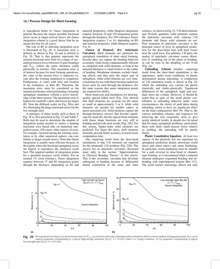
is reproduced better by Gauss integration ingeneral. Because the largest possible fractionalerrors occur at larger tension forces, the Gaussintegration scheme is a good choice (but by nomeans the best for all cases).

The role of R/t in affecting integration erroris illustrated in Fig. 20. A maximum error isdefined, as shown in Fig. 18 and as plotted inFig. 20. That is, this quantity represents theassured fractional error limit for a range of nor-malized tension forces between 0 (pure bending)and Tmax (where the entire thickness yieldsplastically in tension). This maximum error isof interest because for most forming operations,the value of the tension force is unknown ex-cept after the forming simulation is completed.Furthermore, it varies with time and locationin the workpiece, as does R/t. Therefore, themaximum error must be considered as thenumerical tolerance when performing a forming/springback simulation without a priori knowl-edge of the sheet tension. The maximum error ishighest for small R/t values and lowest for largerR/t. Note the different scales on Fig. 20(a) and(b), illustrating the larger fractional errors for thelow-strength steel.

A summary of many results such as those inFig. 18 to 20 is presented in Fig. 21 and Table 5.Both may be used to determine the number ofintegration points needed to assure a limitingfractional error based only on numerical inte-gration errors. (Of course, other sources of error,for example, incurred during the forming simu-lation or by other numerical aspects, can con-tribute to larger overall errors.) Note that Gaussintegration is usually more efficient because, inthe regime where the fractional springback errorsare largest, it reproduces the analytical resultbest. The required number of integration pointsfor a specified accuracy varies widely. For anassured 1% error tolerance, Gauss integrationrequires between 17 and 68 integration pointsthrough the thickness (depending on R/t and

material properties), while Simpson integrationrequires between 35 and 139 integration pointsthrough the thickness. For 10% tolerance, Gaussintegration requires 5 to 16, depending on R/tand material properties, while Simpson requires9 to 41.

Choice of Element, R/t, AnticlasticCurvature. Shell elements are preferred forspringback simulation of sheet metal forming,because they can capture the bending behavioraccurately while being computationally efficientas compared with solid elements, as long at thematerial thickness is small relative to the radiusof bending. Membrane elements exclude bend-ing effects and thus miss the major part ofspringback, while solid elements are very time-consuming for use with sheets because numerouslayers must be used through the thickness (forthe same reasons that many integration pointsare required for shells).

Draw-bend tests and simulations for drawing-quality special killed steel (Fig. 22a) showedthat shell elements are accurate for R/t ratiosas small as approximately 5 or 6, while solidelements are needed for smaller values, atmuch increased cost. Solid elements capture thethrough-thickness stresses that become signifi-cant for small R/t, but the typical brick elementswith linear shape functions are very stiff inbending and provide poor results (Fig. 22b). Forthis reason, higher-order solid elements arepreferred. For larger R/t ratios, shell elementsnormally provide better accuracy at much lowercomputation time.

One surprising result from the draw-bendsimulations is that 3-D elements are requiredfor the nominally 2-D problem (Fig. 22b). Theanswer lies in anticlastic curvature, discussedmore fully in the section “Approximationsin Classical Bending Theory” in this article.This is the secondary curvature that developsorthogonal to bending because of differentiallateral contraction at the inner and outer

surfaces. As shown in Fig. 23, 3-D shell elementsand 20-node quadratic solid elements capturethe anticlastic curvature well, whereas 2-Delements and linear solid elements do not.Poor treatment of anticlastic curvature is theprincipal source of error in springback predic-tion for the draw-bend tests with back forcesnear the yield force. For arbitrary 3-D parts, theanalog of anticlastic curvature causes distor-tion or wrinkling out of the plane of bending,as can be seen in the dimpling of the S-rail(Fig. 1a).

Unloading Scheme. Another surprisingresult from the draw-bend simulations is theimportance, under some conditions, of plasticdeformation during unloading. A comparisonof 2-D simulation results is shown in Fig. 24,where the unloading was carried out purelyelastically and elastic-plastically. Significantdifferences of the springback angle and resi-dual stress are evident. However, it should benoted that in spite of the small plastic con-tribution to unloading behavior under somecircumstances, the choice of path taken duringunloading seems to have no significant effecton the final configuration (Ref 39). That is, thevarious unloading schemes and sequences forremoving the tool constraints seem to givenearly identical results. It should also be notedthat for many springback problems, particularlythose with fairly small tension forces relativeto yielding, the unloading will be purelyelastic.

Plastic Constitutive Equation. At least twoaspects of the plasticity law are important forspringback prediction: plastic anisotropy (yieldstress and strain ratios) and strain hardening.In particular, strain hardening must be suitablefor a path reversal in draw-bend or channel-type forming, as is encountered when a materialelement undergoes sequential bending and un-bending with superimposed tension (Ref 117).The yield surface anisotropy affects not only

0

5

10

15

0

(a)

20 40 60 80 100

Max

imum

err

or, %

R /t R /t

NIP=5

NIP=9

21

3551

15

Gauss integration

0

10

20

30

40

0 20 40

(b)

60 80 100

Max

imum

err

or, %

NIP=5

NIP=9

21

35

51

15

Low-strength steel (Eq 26)0 ≤ T ≤ Tmax

Gauss integration

High-strength aluminum(Eq 27), 0 ≤ T ≤ Tmax

Fig. 20 The maximum error (that is, for sheet tensions from 0 to Tmax) as a function of the ratio of bending radius to thickness (R/t) for various numbers of integration points (NIP). (a) Formaterial properties corresponding to a typical high-strength aluminum (Eq 27, E=70 GPa, where E is Young’s modulus). (b) For properties corresponding to typical

low-strength steel (Eq 26, E=210 GPa)

16 / Process Design for Sheet Forming

Name ///sr-nova/Dclabs_wip/ASM/5120_12R_01-23.pdf/A0005131/ 27/2/2006 5:28PM Plate # 0 pg 16

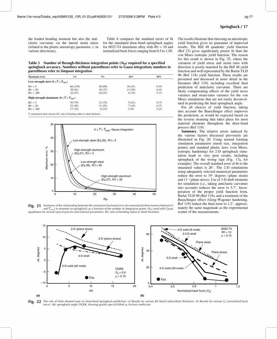
the loaded bending moment but also the anti-clastic curvature via the lateral strain ratios(related to the plastic anisotropy parameter, r, invarious directions).

Table 6 compares the standard errors of fitfor the simulated draw-bend springback anglesfor 6022-T4 aluminum alloy with R/t=10 andnormalized back forces ranging from 0.5 to 1.05.

The results illustrate that choosing an anisotropicyield function gives no guarantee of improvedresults. The Hill 48 quadratic yield function(Ref 23) gives significantly poorer fit than thevon Mises isotropic yield function. The reasonfor this result is shown in Fig. 25, where thevariation of yield stress and strain ratio withdirection is poorly matched by the Hill 48 yieldfunction and well represented by the Barlat YLD96 (Ref 118) yield function. These results arepresented and discussed in more detail in theliterature (Ref 119), including excellent finalprediction of anticlastic curvature. There arelikely compensating effects of the yield stressvariance and strain-ratio variance for the vonMises simulations that are not easily deconvol-uted in predicting the final springback angle.

For all choices of yield function, takinginto account the Bauschinger effect improvesthe prediction, as would be expected based onthe reverse straining that takes place for mostmaterial elements throughout the draw-bendprocess (Ref 119).

Summary. The relative errors induced bythe various factors discussed previously areillustrated in Fig. 26. Using normal formingsimulation parameters (mesh size, integrationpoints) and standard plastic laws (von Mises,isotropic hardening) for 2-D springback simu-lation leads to very poor results, includingspringback of the wrong sign (Fig. 17a, forexample). The overall standard error of fit to themeasured values is 26�. The 2-D simulationsusing adequately selected numerical parametersreduce the error to 19� degrees (plane strain)and 11� (plane stress). Use of 3-D shell elementsfor simulation (i.e., taking anticlastic curvatureinto account) reduces the error to 5.7�. Incor-poration of the proper yield function form,Barlat YLD 96 (Ref 118), and a treatment of theBauschinger effect (Geng-Wagoner hardening,Ref 119) reduce the final error to 1.2�, approxi-mately the same magnitude as the experimentalscatter of the measurements.

Table 5 Number of through-thickness integration points (NIP) required for a specifiedspringback accuracy. Numbers without parentheses refer to Gauss integration; numbers inparentheses refer to Simpson integration

Maximum error 1% 5% 10% 50%

Low-strength steel (0jTjTmax)

R/t=5 68 (139) 26 (69) 16 (41) 4 (9)R/t=20 38 (91) 18 (37) 13 (29) 4 (9)R/t=100 22 (57) 10 (23) 6 (15) 3 (7)

High-strength aluminum (0jTjTmax)

R/t=5 30 (79) 13 (33) 9 (21) 4 (7)R/t=20 22 (55) 11 (25) 7 (15) 4 (7)R/t=100 17 (35) 8 (15) 5 (9) 3 (5)

T , normalized sheet tension; R/t, ratio of bending radius to sheet thickness

0

10

20

30

40

50

0 10 20 30 40 50

Max

imum

err

or, %

NIP

Low-strength steel (Eq 26), R/t = 5

High-strength aluminum(Eq 27), R/t = 5

0 ≤ T ≤ Tmax, Gauss integration

Low-strength steel(Eq 26), R/t = 50

High-strength aluminum(Eq 27), R/t = 35

Fig. 21 Summary of the relationship between the maximum fractional error (for normalized sheet tension between 0and Tmax) in moment (or springback) as a function of the number of integration points (NIP) used with Gauss

quadrature for several typical process and material parameters. R/t, ratio of bending radius to sheet thickness

−10

−5

0

5

10

15

0 5 10 15 20

R/t

∆θ, d

egre

es

DQSKFb = 0.9

3-D shell

3-D solid (20 node)

µ = 0.15

2-D (plane strain)

2-D (plane stress)

Exp.

(a)

0

20

40

60

0.4

(b)

0.6 0.8 1 1.2

Normalized back force (Fb)

∆θ, d

egre

es

Plane strain

Plane stress

3-D shell

3-D solid (8-node)R/t = 10µ = 0.15

3-D solid (20-node)

2.5-D shell

Exp.

6022-T4

Fig. 22 The role of finite element type on draw-bend springback prediction. (a) Results for various R/t (bend radius/sheet thickness). (b) Results for various Fb (normalized backforce). Dh, springback angle; DQSK, drawing quality special killed; m, friction coefficient

Springback / 17

Name ///sr-nova/Dclabs_wip/ASM/5120_12R_01-23.pdf/A0005131/ 27/2/2006 5:28PM Plate # 0 pg 17

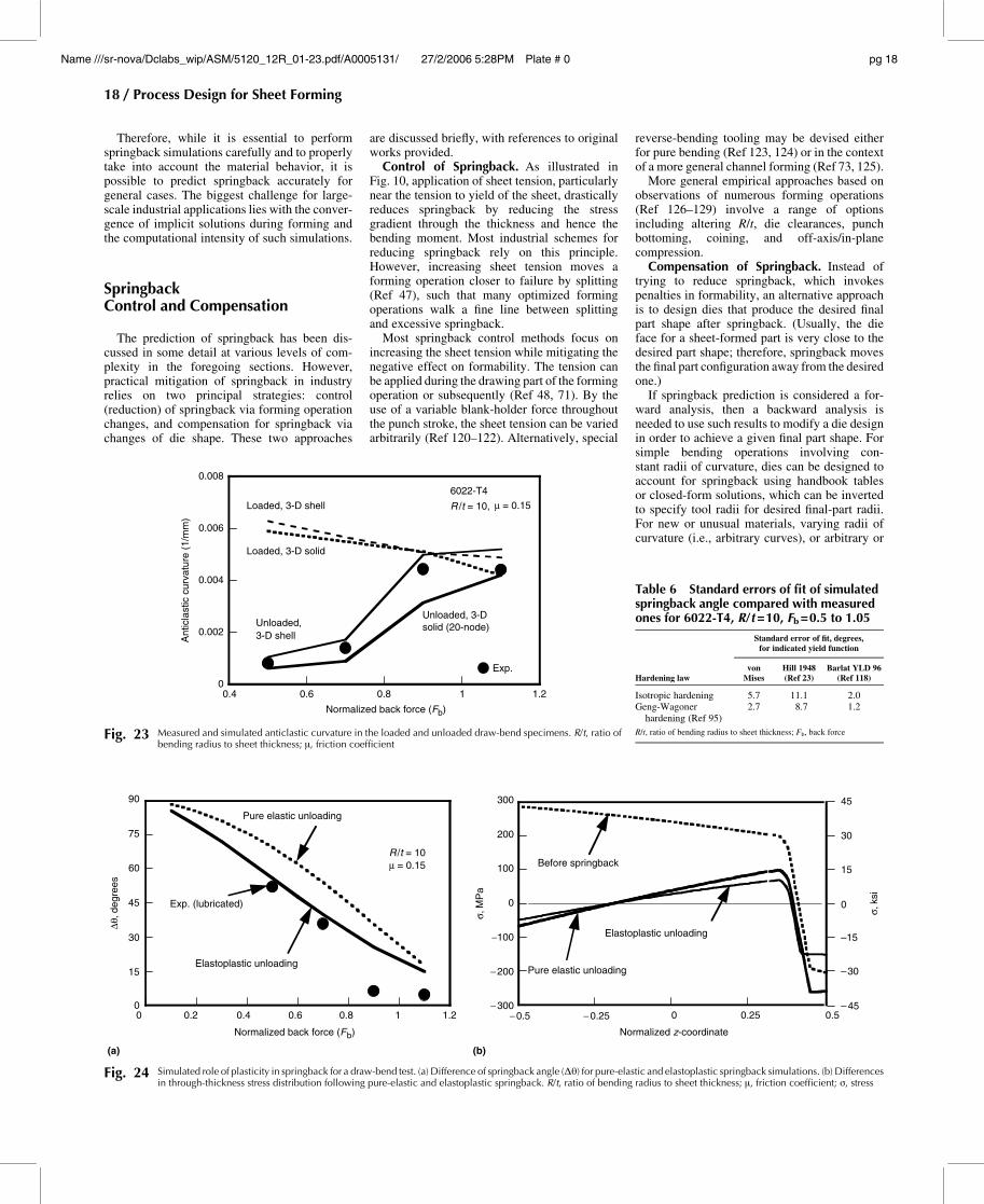
Therefore, while it is essential to performspringback simulations carefully and to properlytake into account the material behavior, it ispossible to predict springback accurately forgeneral cases. The biggest challenge for large-scale industrial applications lies with the conver-gence of implicit solutions during forming andthe computational intensity of such simulations.

SpringbackControl and Compensation

The prediction of springback has been dis-cussed in some detail at various levels of com-plexity in the foregoing sections. However,practical mitigation of springback in industryrelies on two principal strategies: control(reduction) of springback via forming operationchanges, and compensation for springback viachanges of die shape. These two approaches

are discussed briefly, with references to originalworks provided.

Control of Springback. As illustrated inFig. 10, application of sheet tension, particularlynear the tension to yield of the sheet, drasticallyreduces springback by reducing the stressgradient through the thickness and hence thebending moment. Most industrial schemes forreducing springback rely on this principle.However, increasing sheet tension moves aforming operation closer to failure by splitting(Ref 47), such that many optimized formingoperations walk a fine line between splittingand excessive springback.

Most springback control methods focus onincreasing the sheet tension while mitigating thenegative effect on formability. The tension canbe applied during the drawing part of the formingoperation or subsequently (Ref 48, 71). By theuse of a variable blank-holder force throughoutthe punch stroke, the sheet tension can be variedarbitrarily (Ref 120–122). Alternatively, special

reverse-bending tooling may be devised eitherfor pure bending (Ref 123, 124) or in the contextof a more general channel forming (Ref 73, 125).

More general empirical approaches based onobservations of numerous forming operations(Ref 126–129) involve a range of optionsincluding altering R/t, die clearances, punchbottoming, coining, and off-axis/in-planecompression.

Compensation of Springback. Instead oftrying to reduce springback, which invokespenalties in formability, an alternative approachis to design dies that produce the desired finalpart shape after springback. (Usually, the dieface for a sheet-formed part is very close to thedesired part shape; therefore, springback movesthe final part configuration away from the desiredone.)

If springback prediction is considered a for-ward analysis, then a backward analysis isneeded to use such results to modify a die designin order to achieve a given final part shape. Forsimple bending operations involving con-stant radii of curvature, dies can be designed toaccount for springback using handbook tablesor closed-form solutions, which can be invertedto specify tool radii for desired final-part radii.For new or unusual materials, varying radii ofcurvature (i.e., arbitrary curves), or arbitrary or

0

0.002

0.004

0.006

0.008

0.4 0.6 0.8 1 1.2

Ant

icla

stic

cur

vatu

re (

1/m

m)

Normalized back force (Fb)

Loaded, 3-D shell

Unloaded,3-D shell

Unloaded, 3-Dsolid (20-node)

6022-T4

R /t = 10, µ = 0.15

Loaded, 3-D solid

Exp.

Fig. 23 Measured and simulated anticlastic curvature in the loaded and unloaded draw-bend specimens. R/t, ratio ofbending radius to sheet thickness; m, friction coefficient

0

15

30

45

60

75

90

0 0.2

(a)

0.4 0.6 0.8 1 1.2

Normalized back force (Fb)

∆θ, d

egre

es

R /t = 10µ = 0.15

Pure elastic unloading

Elastoplastic unloading

Exp. (lubricated)

−300

−200

−100

0

100

200

300

– 45

–30

–15

0

15

30

45

−0.5

(b)

−0.25 0.25 0.5

Normalized z-coordinate

σ, M

Pa

σ, k

siBefore springback

Pure elastic unloading

Elastoplastic unloading

0

Fig. 24 Simulated role of plasticity in springback for a draw-bend test. (a) Difference of springback angle (Dh) for pure-elastic and elastoplastic springback simulations. (b) Differencesin through-thickness stress distribution following pure-elastic and elastoplastic springback. R/t, ratio of bending radius to sheet thickness; m, friction coefficient; s, stress

Table 6 Standard errors of fit of simulatedspringback angle compared with measuredones for 6022-T4, R/t =10, Fb =0.5 to 1.05

Hardening law

Standard error of fit, degrees,for indicated yield function

vonMises

Hill 1948(Ref 23)

Barlat YLD 96(Ref 118)

Isotropic hardening 5.7 11.1 2.0Geng-Wagoner

hardening (Ref 95)2.7 8.7 1.2

R/t, ratio of bending radius to sheet thickness; Fb, back force

18 / Process Design for Sheet Forming

Name ///sr-nova/Dclabs_wip/ASM/5120_12R_01-23.pdf/A0005131/ 27/2/2006 5:28PM Plate # 0 pg 18

3-D shapes (with compound curvature), spring-back compensation has traditionally been carriedout by simple trial and error or some variationthereof (Ref 130–132). Unfortunately, this pro-cedure often produces unsatisfactory results anddepends intimately on the skill and experienceof the user. The process can take many months,thus extending critical tooling lead times. Thetrial-and-error method can be applied using FEforward analysis trials instead of experiments,but the backward design steps are equally in-efficient and may take a similar amount of time.

Schemes for guiding the forward and back-ward analyses may be found in the literaturebased on various optimization strategies (Ref 89,133, 134). These methods typically involve agradient calculation and sensitivity analyses.Considerable complexity in formulation andimplementation is involved, and usually specialprogramming within special-purpose FE pro-grams is required.

A promising approach integrating forward(FE) and backward analyses in an iterativescheme was reported by Karafillis and Boyce

(Ref 135–137). This method, denoted the spring-forward method, may in principle be usedwith any FE program. As discussed subse-quently, however, its application suffers fromlack of convergence (Ref 138, 139) unless theforming operation is symmetric or has verylimited geometric change during springback(Ref 138).

Figure 27 outlines the steps of the spring-forward method. A flat sheet is first deformedinto the target shape, and the external forces arerecorded. At step 3, the target shape is elastically

0

0.2

0.4

0.6

0.8

1

0 15

(a)

30 45 60 75 90

r-va

lue

Angle from the rolling direction, degrees

Barlat YLD 96(Ref 93)

Hill 48(Ref 20)

Barlat YLD 8(Ref 92)

von Mises

6022-T4Exp.

0.9

0.95

1

1.05

1.1

0 15

(b)

30 45 60 75 90

Nor

mal

ized

yie

ld s

tres

s

Angle from the rolling direction, degrees

Barlat YLD 96

Barlat YLD 89

Hill 48

von Mises

Exp.

6022-T4

Fig. 25 Comparison of plasticity predictions for various in-plane sheet directions for several yield functions fit to a 6022-T4 aluminum alloy sheet. (a) Plastic anisotropy parameter(r-value). (b) Yield stresses normalized to yield stress in the rolling direction (0�)

0

20

40

60

0.4 0.6 0.8 1.2

∆θ, d

egre

es

Normalized back force (Fb)

6022-T4R/t = 10µ = 0.15

Exp.

(2) <σ> = 19°

(1) <σ> = 26°

(3) <σ> = 11°

(4) <σ> = 5.7°

(5) <σ> = 1.2°

1

Fig. 26 The role of numerical procedures and constitutive modeling in springbackaccuracy as represented by standard error of fit,5s4, to measurement.

Springback angles (Dh): (1) Plane stress, 5 integration points (NIP), 600 elements alonglength (NEL), von Mises yield, and isotropic hardening. (2) Plane strain, NIP=51,NEL=600, von Mises yield, and isotropic hardening. (3) Plane stress, NIP=51,NEL=600, von Mises yield, and isotropic hardening. (4) 3-D shell, NIP=51, NEL=600,von Mises yield, and isotropic hardening. (5) 3-D shell, NIP=51, NEL=600, Barlat 96yield, and Geng-Wagoner anisotropic hardening. R/t, ratio of bending radius to sheetthickness; m, friction coefficient

(i+1)th trial after springback

Flat sheet

Target

→X t

iool

→

→

X tool

Fexternal

i+1

1)

Steps

2)

3)

4)

Fig. 27 Schematic representation of the steps undertaken in the springforward methodof springback compensation. Step 1: flat sheet before deformation; Step 2: form

to the tool shape and record external force field; Step 3: apply the recorded force field to theprevious tooling shape and obtain the new tooling shape; Step 4: evaluate the (i+1)th toolingshape by comparing the part shape, after forming and springback, with the target shape.xi

tool, forming tool position at i th iteration; F, force. Source: Ref 135–137

Springback / 19

Name ///sr-nova/Dclabs_wip/ASM/5120_12R_01-23.pdf/A0005131/ 27/2/2006 5:28PM Plate # 0 pg 19

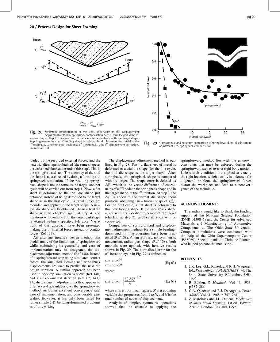
loaded by the recorded external forces, and thenext trial die shape is obtained (the same shape asthe deformed blank at the end of this step). This isthe springforward step. The accuracy of the trialdie shape is next checked by doing a forming andspringback simulation. If the resulting spring-back shape is not the same as the target, anothercycle will be carried out from step 1. Now, a flatsheet is deformed to the trial die shape justobtained, instead of being deformed to the targetshape as in the first cycle. External forces arerecorded and applied to the target shape. A newtrial die shape will be obtained. The new trial dieshape will be checked again at step 4, anditerations will continue until the target part shapeis attained within a specified tolerance. Varia-tions of this approach have been presentedmaking use of internal forces instead of contactforces (Ref 137).

An alternate iterative design method thatavoids many of the limitations of springforwardwhile maintaining its generality and ease ofimplementation may be designated the dis-placement adjustment method (Ref 138). Insteadof a springforward step using simulated contactforces, the simulated forming and springbackdisplacements are used to predict the next diedesign iteration. A similar approach has beenused in one-step simulation versions (Ref 140)and via experimental iteration (Ref 67, 141).The displacement adjustment method appears tooffer several advantages over the springforwardmethod, including excellent convergence rate,ease of implementation, and considerable gen-erality. However, it has only been tested forrather simple 2-D, bending-dominated problemsas of this writing.

The displacement adjustment method is out-lined in Fig. 28. First, a flat sheet of metal isdeformed to a trial die shape (for the first cycle,the trial die shape is the target shape). Afterspringback, the springback shape is comparedwith its target. The shape error is defined asD~y i, which is the vector difference of coordi-nates of a FE node in the springback shape and inthe target shape, at the ith iteration. At step 3, theD~y i is added to the current die shape nodalpositions, obtaining a new tooling shape of~X i+1

tool .For the next cycle, a flat sheet is deformed tothis new tooling shape. If the springback shapeis not within a specified tolerance of the target(checked at step 2), another iteration will beconducted.

Comparison of springforward and displace-ment adjustment methods for a simple bending-dominated forming operation have been pres-ented (Ref 138). For an arbitrary, nonsymmetric,nonconstant-radius part shape (Ref 138), bothmethods were applied, with iterative resultsshown in Fig. 29. The normalized error for thenth iteration cycle in Fig. 29 is defined as:

rms error(n)

rms error(1)(Eq 63)

where:

rms error=P

D~y 2k

N

� �1=2

(Eq 64)

where rms is root mean square, K is a countingvariable that progresses from 1 to N, and N is thetotal number of nodes of displacement.

Analysis of simpler, symmetric operationsshowed that the obstacle to applying the

springforward method lies with the unknownconstraints that must be enforced during thespringforward step to restrict rigid body motion.Unless such conditions are applied at exactlythe right location, which usually is unknown fora general problem, the springforward forcesdistort the workpiece and lead to nonconver-gence of the technique.

ACKNOWLEDGMENTS

The authors would like to thank the fundingsupport of the National Science Foundation(DMR 0139045) and the Center for AdvancedMaterials and Manufacturing of AutomotiveComponents at The Ohio State University.Computer simulations were conducted withthe help of the Ohio Supercomputer Center(PAS080). Special thanks to Christine Putnam,who helped prepare the manuscript.

REFERENCES

1. J.K. Lee, G.L. Kinzel, and R.H. Wagoner,Ed., Proceedings of NUMISHEET ’96, TheOhio State University (Columbus, OH),1996

2. R. Boklen, Z. Metallkd., Vol 44, 1953,p 382–386

3. C.A. Queener and R.J. DeAngelis, Trans.ASME, Vol 61, 1968, p 757–768

4. Z. Marciniak and J.L. Duncan, Mechanicsof Sheet Metal Forming, 1st ed., EdwardArnold, London, England, 1992

1)

Steps

2)

3)

Target

= +

→X t

iool

→X t

iool

→

→X t

iool

i+1→X tool

→X tool

i+1

y i

∇

→y i

∇

→y i

∇

Tool

Tool

Fig. 28 Schematic representation of the steps undertaken in the DisplacementAdjustment method of springback compensation. Step 1: form the part to the i th

tooling shape; Step 2: compare the part shape after springback with the target shape;Step 3: generate the (i+1)th tooling shape by adding the displacement error field to thei th tooling. xi

tool, forming tool position at i th iteration; Dy i, the i th displacement correction.Source: Ref 138

0.0

0.2

0.4

0.6

0.8

1.0

50 10 15 20 25

Nor

mal

ized

err

or

Number of cycles

DA

Springforward

Fig. 29 Convergence and accuracy comparison of springforward and displacementadjustment (DA) springback compensation

20 / Process Design for Sheet Forming

Name ///sr-nova/Dclabs_wip/ASM/5120_12R_01-23.pdf/A0005131/ 27/2/2006 5:28PM Plate # 0 pg 20

5. Z. Marciniak, J.L. Duncan, and S.J. Hu,Mechanics of Sheet Metal Forming, 2nded., Butterworth-Heinemann, 2002

6. W.F. Hosford and R.M. Caddell, MetalForming: Mechanics and Metallurgy, 2nded., Prentice Hall, 1993

7. K.C. Chan and S.H. Wang, J. Mater.Process. Technol., Vol 91, 1999,p 111–115

8. W. Schroeder, J. Appl. Mech. (Trans.ASME), Vol 65, 1943, p 817–827

9. T.X. Yu and L.C. Zhang, Plastic Bending,Theory and Applications, World Scientific,1996

10. W.C. Young, Table I, Case 20, Roark’sFormulas for Stress and Strain, 6th ed.,McGraw-Hill, 1989, p 68

11. B.W. Shaffer and E.E. Ungar, J. Appl.Mech. (Trans. ASME), Vol 82, 1960,p 34–40

12. S.H. Crandall and N.C. Dahl, Introductionto the Mechanics of Solids, McGraw-Hill,1961, p 327–336

13. J.D. Lubahn and G. Sachs, Trans. ASME,Vol 72, 1950, p 201–208

14. F.J. Gardiner, J. Appl. Mech. (Trans.ASME), Vol 79, 1957, p 1–9

15. J.M. Alexander, An Analysis of the PlasticBending of Wide Plate, and the Effect ofStretching on Transverse Residual Stress,Proc. Inst. Mech. Eng., Vol 173 (No. 1),1959, p 73–96

16. G. Sachs, Principles and Methods of Sheet-Metal Fabricating, Reinhold, 1951

17. J.H. Hollomon, A.I.M.E. Trans., Vol 162,1945, p 268

18. D.M. Woo and J. Marshall, The Engineer,Vol 208, 1959, p 135–136

19. Z.T. Zhang and S.J. Hu, “MathematicalBending in Plane Strain Bending,” Paper970439, Society of Automotive Engineers,1997

20. User Manual, ABAQUS Standard, Version6.2, ABAQUS, Inc., Pawtucket, RI, 2002

21. A.K. Sachdev and R.H. Wagoner, UniaxialStrain Hardening at Large Strain in SeveralSheet Steels, J. Appl. Metalwork., Vol 3(No. 1), 1983, p 32

22. Properties of Some Metals and Alloys, 3rded., The International Nickel Company,Inc., 1968, p 14

23. R. Hill, Theory of Yielding and PlasticFlow of Anisotropic Metals, Proc. R. Soc.(London), 1948, p 193–281

24. Z.T. Zhang and D. Lee, “Effect of ProcessVariables and Material Properties onthe Springback Behavior of 2-D DrawBending Parts,” Paper 950692, Society ofAutomotive Engineers, 1995

25. E.A. Popov, Russ. Eng. J., Vol 43 (No. 10),1963, p 39–40

26. H. Lamb, Philos. Mag., Vol 31, 1891,p 182–195

27. H.D. Conway and W.E. Nickols, Exp.Mech., Vol 5, 1965, p 115–119

28. D.G. Ashwell, J. R. Aero. Soc., Vol 54,1950, p 708–715

29. D. Horrocks and W. Johnson, Int. J. Mech.Sci., Vol 9, 1967, p 835–861

30. G.F.C. Searle, Experimental Elasticity: AManual for the Laboratory, CambridgeUniversity Press, Cambridge, England,1908

31. J. Case, Strength of Materials, 3rd ed.,Arnold, 1938, p 645–654

32. C.T. Wang, G. Kinzel, and T. Altan,J. Mater. Process. Technol., Vol 39, 1993,p 279–304

33. R. Hill, The Mathematical Theory ofPlasticity, Oxford University Press,London, England, 1950

34. R.H. Wagoner, Metall. Trans. A, Vol 11,1980, p 165–175

35. R.H. Wagoner, Metall. Trans. A, Vol 12,1981, p 2142–2145

36. T.X. Yu and W. Johnson, J. Mech. Work.Technol., Vol 6, 1982, p 5–21

37. K.P. Li and R.H. Wagoner, Simulationof Springback, Simulation of MaterialsProcessing, Proceedings of NUMIFORM’98 (Enschede, Netherlands), 1998, p21–31

38. K.P. Li, L.M. Geng, and R.H. Wagoner,Simulation of Springback: Choice ofElement, Advanced Technology of Plasti-city, Proceedings of the Sixth ICTP(Nuremberg, Germany), Vol III, 1999a,p 2091–2098

39. K.P. Li, L.M. Geng, and R.H. Wagoner,Simulation of Springback with the Draw/Bend Test, Proceedings of IPMM ’99(Vancouver, B.C., Canada), 1999b, p 1

40. K.P. Li, W.P. Carden, and R.H.Wagoner, Int. J. Mech. Sci., Vol 44, 2002,p 103–122

41. R.H. Wagoner, W.D. Carden, W.P.Carden, and D.K. Matlock, Springbackafter Drawing and Bending of MetalSheets, Proceedings, IPMM ’97—Intelli-gent Processing and Manufacturing ofMaterials, University of Wollongong,Vol 1, 1997, p 1–10

42. J.F. Wang, R.H. Wagoner, and D.K.Matlock, Creep following Springback,Proceedings, Tenth Conference of Plasti-city (Quebec City, Canada), 2003, p211–213

43. R.M. Cleveland and A.K. Ghosh, Int. J.Plast., Vol 28, 2002, p 769–785

44. F. Morestin and M. Boivin, Nucl. Eng.Des., Vol 162, 1996, p 107–116

45. H.W. Swift, Engineering, Oct 1948,p 333–359

46. M.L. Wenner, Report MA-233, GeneralMotors Research Laboratories, May 1982

47. M.L. Wenner, J. Appl. Metalwork., Vol 2(No. 4), 1983, p 277–287

48. M.K. Mickalich and M.L. Wenner, ReportGMR-6108, General Motors ResearchLaboratories, Feb 1988

49. J.L. Duncan and J.E. Bird, Approximatecalculations for Draw Die Forming andTheir Application to Aluminium AlloySheet, Proceedings of the Tenth Biennial

Cong. IDDRG, (Warwick, England), Vol 1,The International Deep Drawing ResearchGroup, April 1978, p 45–52

50. J.L. Duncan and J.E. Bird, Sheet Met. Ind.,Vol 55 (No. 9), Sept 1978, p 1015–1023

51. T. Kuwabara, S. Takahashi, K. Akiyama,and Y. Miyashita, “2-D SpringbackAnalysis for Stretch-Bending ProcessesBased on Total Strain Theory,” Paper950691, Society of Automotive Engineers,1995, p 1–10

52. T. Kuwabara, S. Takahashi, and K. Ito,Springback Analysis of Sheet MetalSubjected to Bending-Unbending underTension I, Advanced Technology ofPlasticity, Proceedings of the FifthICTP (Columbus, OH), Vol 2, 1996,p 743–746

53. S. Takahashi, T. Kuwabara, and K. Ito,Springback Analysis of Sheet MetalSubjected to Bending-Unbending underTension II, Advanced Technology ofPlasticity, Proceedings of the Fifth ICTP(Columbus, OH), Vol 2, 1996, p 747–750

54. T. Kuwabara, N. Sekiand, and S.Takahashi, A Rigorous Numerical Analy-sis of Residual Curvature of Sheet MetalsSubjected to Bending-Unbending underTension, Advanced Technology of Plasti-city, Proceedings of the Sixth ICTP(Nuremberg, Germany), Vol 2, 1999,p 1071–1076

55. W.Y.D. Yuen, J. Mater. Process. Technol.,Vol 22, 1990, p 1–20

56. R. Hino, Y. Goto, and M. Shiraishi,Springback of Sheet Metal LaminatesSubjected to Stretch Bending and theSubsequent Unbending, Advanced Tech-nology of Plasticity, Proceedings of theSixth ICTP (Nuremberg, Germany), Vol 2,Sept 19–24, 1999, p 1077–1082

57. A.A. El-Domiaty, M.A.N. Shabara, andM.D. Al-Ansary, Int. J. Mach. ToolsManuf., Vol 36 (No. 5), 1996, p 635–650

58. W. Johnson and T.X. Yu, Int. J. Mech. Sci.,Vol 23, 1981, p 687–696

59. C. Sudo, M. Kojima, and T. Matsuoka,Some Investigations on Elastic Recoveryof Press Formed Parts of High StrengthSteel Sheets, Proceedings of the EighthBiennial Congress of IDDRG (Gothen-burg, Sweden), Vol 2, The InternationalDeep Drawing Research Group, Sept 1974,p 192–202

60. M.L. Chakhari and J.N. Jalinier, Spring-back of Complex Parts, Proceedings ofthe 13th Biennial Congress of IDDRG(Melbourne, Australia), The InternationalDeep Drawing Research Group, Feb 1984,p 148–159

61. L.C. Zhang and Z. Lin, J. Mater. Process.Technol., Vol 63, 1997, p 49–54

62. A. Focellese, L. Fratini, F. Gabrielli, andF. Micari, J. Mater. Process. Technol., Vol80–81, 1998, p 108–112

63. H. Ogawa and A. Makinouchi, SmallRadius Bending of Sheet Metal by

Springback / 21

Name ///sr-nova/Dclabs_wip/ASM/5120_12R_01-23.pdf/A0005131/ 27/2/2006 5:28PM Plate # 0 pg 21

Indentation with V-Shape Punch, Advan-ced Technology of Plasticity, Proceedingsof the Sixth ICTP (Nuremberg, Germany),Vol 2, Sept 19–24, 1999, p 1059–1064

64. B.S. Levy, J. Appl. Metalwork., Vol 3(No. 2), 1984, p 135–141

65. S.S. Han and K.C. Park, An Investigationof the Factors Influencing Springback byEmpirical and Simulative Techniques,Proceedings of NUMISHEET ’99(Besancon, France), 1999, p 53–57

66. L.R. Sanchez, D. Robertson, and J.C.Gerdeen, “Springback of Sheet Metal Bentto Small Radius/Thickness Ratios,” Paper960595, Society of Automotive Engineers,1996, p 650–656

67. C. Wang, An Industrial Outlook forSpringback Predictability, MeasurementReliability, and Compensation Technol-ogy, Proceedings of NUMISHEET 2002(Jeju Island, Korea), 2002, p 597–604

68. R.G. Davies, J. Appl. Metalwork., Vol 1,(No. 4), 1981, p 45–52

69. F. Pourboghrat and E. Chu, Int. J.Mech. Sci., Vol 36 (No. 3), 1995, p 327–341

70. F. Pourboghrat and E. Chu, J. Mater. Pro-cess. Technol., Vol 50, 1995, p 361–374

71. R.G. Davies, J. Appl. Metalwork., Vol 3(No. 2), 1984, p 120–126

72. N.E. Thompson and C.H. Ellen, J. Appl.Metalwork., Vol 4 (No. 1), 1985, p 39–42

73. Y.C. Liu, J. Eng. Mater. Technol. (Trans.ASME), Vol 110, 1988, p 389–394

74. W.D. Carden, L.M. Geng, D.K. Matlock,and R.H. Wagoner, Int. J. Mech. Sci., Vol44, 2002, p 79–101

75. A. Makinouchi, E. Nakamachi, E. Onate,and R.H. Wagoner, Ed., Proceedings ofNUMISHEET ’93 (Isehara, Japan), TheInstitute of Physical and ChemicalResearch, 1993

76. S.F. Shen and P.R. Dawson, Ed., Simula-tion of Materials Processing: Theory,Methods and Applications, A.A. Balkema,Rotterdam, Holland, 1995

77. J.C. Gelin and P. Picart, Ed., Proceedingsof NUMISHEET ’99 (Besancon, France),Burs Publications, 1999

78. D.-Y. Yang, S.I. Oh, H. Huh, and Y.H.Kim, Ed., NUMISHEET 2002—Proc. FifthInt. Conf. Workshop Num. Simul. 3D SheetForming Processes (Jeju, Korea), Vol 1,2002

79. K. Mattiasson, A. Strange, P. Thilderkvist,and A. Samuelsson, Simulation of Spring-back in Sheet Metal Forming, Proceedingsof the Fifth International Conference onNumerical Methods in Industrial FormingProcess (New York), 1995, p 115–124

80. S.W. Lee and D.Y. Yang, J. Mater. Pro-cess. Technol., Vol 80–81, 1998, p 60–67

81. S.C. Tang, Analysis of Springback in SheetForming Operation, Advanced Technologyof Plasticity, Proceedings, Second ICTP(Stuttgart, Germany), Vol 1, 1987, p193–197

82. N. He and R.H. Wagoner, SpringbackSimulation in Sheet Metal Forming, Pro-ceedings of NUMISHEET ’96 (Columbus,OH), 1996, p 308–315

83. N. Narasimhan and M. Lovell, Finite Elem.Anal. Des., Vol 33, 1999, p 29–42

84. Y. Hu and C. Du, Quasi Static FiniteElement Algorithms for Sheet MetalStamping Springback Simulation, Pro-ceedings of NUMISHEET ’99 (Besancon,France), 1999, p 71–76

85. L.M. Geng and R.H. Wagoner, SpringbackAnalysis with a Modified HardeningModel, Sheet Metal Forming, Sing Tang65th Anniversary Volume, SP-1536, SAEPublication 2000-01-0768, Society ofAutomotive Engineers, 2000, p 21–32

86. D.W. Park, J.J. Kang, J.P. Hong, and S.I.Oh, Springback Simulation by Com-bined Method of Explicit and ImplicitFEM, Proceedings of NUMISHEET ’99(Besancon, France), 1999, p 35–40

87. F. Valente and D. Traversa, SpringbackCalculation of Sheet Metal Parts afterTrimming and Flanging, Proceedings ofNUMISHEET ’99 (Besancon, France),1999, p 59–64

88. N. Montmayeur and C. Staub, SpringbackPrediction with OPTRIS, Proceedings ofNUMISHEET ’99 (Besancon, France),1999, p 41–46

89. G.Y. Li, M.J. Tan, and K.M. Liew, Int. J.Solids Struct., Vol 36 (No. 30), Oct 1999,p 4653–4668

90. U. Abdelsalam, A. Sikorski, and M. Kar-ima, Application of One Step Springbackfor Product and Early Process Feasibilityon Sheet Metal Stampings, Proceedings ofNUMISHEET ’99 (Besancon, France),1999, p 47–52

91. R.H. Wagoner and J.-L. Chenot, MetalForming Analysis, Cambridge UniversityPress, Cambridge, U.K., 2001

92. R.D. Cook, D.R. Malkus, M.E. Plesha,R.J. Witt, Concepts and Applications ofFinite Element Analysis, 4th ed., Wiley,2002

93. J.N. Reddy, Introduction to the FiniteElement Method, 2nd ed., McGraw-Hill,1993

94. O.C. Zienkiewicz and R.L. Taylor, TheFinite Element Method: Volume 1, TheBasis, 5th ed., Butterworth-Heinemann,Oxford, U.K., 2000

95. O.C. Zienkiewicz and R.L. Taylor, TheFinite Element Method: Volume 2, SolidMechanics, 5th ed., Butterworth-Heinemann, Oxford, U.K., 2000

96. T.J.R. Hughes, The Finite ElementMethod: Linear Static and DynamicAnalysis, Prentice-Hall, 1987

97. K.-J. Bathe, Finite Element Procedures,Prentice-Hall, 1995

98. http://www.abaqus.com/products/products_standard.html, ABAQUS, Inc., 2005

99. http://www.ansys.com/products/mechanical.asp, ANSYS, Inc., 2005

100. http://www.abaqus.com/products/products_explicit.html, ABAQUS, Inc., 2005

101. http://www.lstc.com, Livermore SoftwareTechnology Corp., 2005

102. J. Wang and R.H. Wagoner, A NewHexahedral Solid Element for 3D FEMSimulation of Sheet Metal Forming, Proc.of NUMIFORM 2004, Materials Proces-sing and Design (Columbus, OH), S.Ghosh, J.M. Casto, and J.K. Lee, Ed., June2004, p 2181–2186

103. J. Wang and R.H. Wagoner, A PracticalLarge Strain Solid Finite Element for SheetForming, Int. J. Numer. Methods Eng., inpress

104. T. Shimizu, E. Massoni, N. Soyris, andJ.-L. Chenot, A Modified 3-DimensionalFinite Element Model for Deep-DrawingAnalysis, Advances in Finite DeformationProblems in Material Processing andStructure, N. Chandra et al., Ed., AMD Vol125, ASME, 1991, p 113–118

105. M. Kawka and A. Makinouchi, FiniteElement Simulation of Sheet Metal Form-ing Processes by Simultaneous Use ofMembrane, Shell and Solid Elements,Numerical Methods in Industrial FormingProcesses, J.-L. Chenot et al., Ed.,Balkema, Rotterdam, 1992, p 491–496

106. K.P. Li and R.H. Wagoner, Simulationof Deep Drawing with Various Ele-ments, Proceedings of NUMISHEET ’99(Besancon, France), 1999, p 151–156

107. A. Andersson and S. Holmberg, Simulationand Verification of Different ParametersEffect on Springback Results, Proceedingsof NUMISHEET 2002 (Jeju Island, Korea),2002, p 201–206

108. V.T. Nguyen, Z. Chen, et al., Prediction ofSpring-Back in Anisotropic Sheet Metals,Proc. Inst. of Mech. Eng. C, J. Mech. Eng.Sci., Vol 218 (No. 6), 2004, p 651–661

109. W.L. Xu, C.H. Ma, et al., Sensitive Factorsin Springback Simulation for Sheet MetalForming, J. Mater. Process. Technol., Vol151 (No. 1–3), 2004, p 217–222

110. N. Yamamura, T. Kuwabara, et al., Spring-back Simulations for Stretch-Bending andDraw-Bending Processes Using the StaticExplicit FEM Code, with an Algorithm forCanceling Non-equilibrated Forces, Pro-ceedings of NUMISHEET 2002 (JejuIsland, Korea), 2002, p 25–30

111. H. Yao, S.-D. Liu, et al., Techniques toImprove Springback Prediction AccuracyUsing Dynamic Explicit FEA Codes, SAETrans. J. Mater. Manuf., Vol 111, 2002,p 100–106

112. R.H. Wagoner and M. Li, Advances inUnderstanding Springback Simulations,Proceedings of NUMISHEET 2005, 2005

113. R.H. Wagoner and M. Li, Sheet Simula-tion of Springback: Through-ThicknessIntegration, Int. J. Numer. Methods Eng.,submitted

114. E.W. Weisstein, Trapezoidal Rule, Math-World—A Wolfram Web Resource, http://

22 / Process Design for Sheet Forming

Name ///sr-nova/Dclabs_wip/ASM/5120_12R_01-23.pdf/A0005131/ 27/2/2006 5:28PM Plate # 0 pg 22

mathworld.wolfram.com/TrapezoidalRule.html, 2005

115. E.W. Weisstein, Simpson’s Rule, Math-World—A Wolfram Web Resource, http://mathworld.wolfram.com/SimpsonsRule.html, 2005

116. E.W. Weisstein, Legendre-Gauss Quad-rature, MathWorld—A Wolfram WebResource, http://mathworld.wolfram.com/Legendre-GaussQuadrature.html, 2005

117. S.C. Tang, Application of an Aniso-tropic Hardening Rule to SpringbackPrediction, Advanced Technology ofPlasticity, Proceedings, Fifth ICTP(Columbus, OH), Vol 2, 1996, p 719–722

118. F. Barlat, Y. Maeda, K. Chung, M. Yana-gawa, J.C. Brem, Y. Hayashida, D.J. Legfe,S.J. Matsui, S.J. Murtha, S. Hattori, R.C.Becker, and S. Makosey, J. Mech. Phys.Solids. Vol 45 (No. 11/12), 1997, p 1727–1763

119. L.M. Geng and R.H. Wagoner, Int.J. Mech. Sci., Vol 44, 2002, p 123–148

120. Y. Hishida and R.H. Wagoner, SAE paper930285, J. Mater. Manuf., Vol 102, 1993,p 409–415

121. D. Schmoeckel and M. Beth, Ann. CIRP,Vol 42 (No. 1), 1993, p 339–342

122. M. Sunseri, J. Cao, A.P. Karafillis, andM.C. Boyce, Trans. ASME, Vol 118, 1996,p 426–435

123. C.C. Chu, Int. J. Solids Struct., Vol 22(No. 10), 1986, p 1071–1081

124. Y. Nagai, Jpn. Soc. Technol. Plast., Vol 28,1987, p 143–149

125. R.A. Ayres, J. Appl. Metalwork., Vol 3(No. 2), 1984, p 127–134

126. Y. Hayashi, Analysis of Surface Defectsand Side Wall Curl in Press Forming,Proceedings of the 13th Biennial Congressof IDDRG (Melbourne, Australia), TheInternational Deep Drawing ResearchGroup, Feb 1984, p 565–580

127. Y. Tozawa, J. Mater. Process. Technol.,Vol 22, 1990, p 343–351

128. Y. Umehara, J. Mater. Process. Technol.,Vol 22, 1990, p 239–256

129. M. Ueda and K. Ueno, J. Mech. Work.Technol., Vol 5, 1981, p 163–179

130. R.D. Webb, “Spatial Frequency BasedClosed-Loop Control of Sheet MetalForming,” Ph.D. thesis, MassachusettsInstitute of Technology, 1987

131. R.D. Webb and D.E. Hardt, J. Eng. Ind.(Trans. ASME ), Vol 113, 1991, p 44–52

132. C. Hindman and K.B. Ousterhout, J.Mater. Process. Technol., Vol 99, 2000,p 38–48

133. O. Ghouati, D. Joannic, and J.C. Gelin,Optimisation of Process Parameters for theControl of Springback in Deep Drawing,Proceedings of NUMIFORM ’98 (Nether-lands), 1998, p 819–824

134. I. Chou and C. Hung, Int. J. Mach. ToolsManuf., Vol 39, 1999, p 517–536

135. A.P. Karafillis and M.C. Boyce, Int.J. Mech. Sci., Vol 34 (No. 2), 1992,p 113–131

136. A.P. Karafillis and M.C. Boyce, J. Mater.Process. Technol., Vol 32, 1992, p499–508

137. A.P. Karafillis and M.C. Boyce, Int. J.Mach. Tools Manuf., Vol 36 (No. 4), 1996,p 503–526

138. W. Gan and R.H. Wagoner, Die DesignMethod for Sheet Springback, Int. J.Mech. Sci., Vol 46 (No. 7), 2004,p 1097–1113

139. R. Lingbeek, J. Huetink, S. Ohnimus, M.Petzoldt, and J. Weiher, The Develop-ment of a Finite Elements Based Spring-back Compensation Tool for Sheet MetalProducts, J. Manuf. Prod. Technol., inpress

140. F. Valente, X.P. Li, and A. Messina, inProceedings of Fourth COMPLAS(Barcelona, Spain), Vol 2, 1997, p1431–1488

141. E. Chu, L. Zhang, S. Wang, X. Zhu,and B. Maker, Validation of Spring-back Predictability with ExperimentalMeasurements and Die Compensationfor Automotive Panels, Proceedings ofNUMISHEET 2002 (Jeju Island, Korea),2002, p 313–318

Springback / 23

Name ///sr-nova/Dclabs_wip/ASM/5120_12R_01-23.pdf/A0005131/ 27/2/2006 5:28PM Plate # 0 pg 23