Embed Size (px)
Citation preview
Vol. 45, No. 2, Spring 2011 85
Chemical Engineering Education Volume 45 Number 2 Spring 2011
CHEMICAL ENGINEERING EDUCATION (ISSN 0009-2479) is published quarterly by the Chemical Engi neering Division, American Society for Engineering Education, and is edited at the University of Florida. Cor respondence regarding editorial matter, circulation, and changes of address should be sent to CEE, Chemical Engineering Department, University of Florida, Gainesville, FL 32611-6005. Copyright © 2011 by the Chemical Engineering Division, American Society for Engineering Education. The statements and opinions expressed in this periodical are those of the writers and not necessarily those of the ChE Division, ASEE, which body assumes no responsibility for them. Defective copies re placed if notified within 120 days of pub lication. Write for information on subscription costs and for back copy costs and availability. POSTMAS TER: Send address changes to business address: Chemical Engineering Education, PO Box 142097, Gainesville, FL 32614-2097. Periodicals Postage Paid at Gainesville, Florida, and additional post offices (USPS 101900).
PUBLICATIONS BOARD
EDITORIAL ADDRESS:Chemical Engineering Education
c/o Department of Chemical Engineering723 Museum Road
University of Florida • Gainesville, FL 32611PHONE and FAX: 352-392-0861
e-mail: [email protected]
EDITOR Tim Anderson
ASSOCIATE EDITORPhillip C. Wankat
MANAGING EDITORLynn Heasley
PROBLEM EDITORDaina Briedis, Michigan State
LEARNING IN INDUSTRY EDITORWilliam J. Koros, Georgia Institute of Technology
• CHAIR •C. Stewart SlaterRowan University
• VICE CHAIR•Jennifer Curtis
University of Florida
• PAST CHAIR •John O’Connell
University of Virginia
• MEMBERS •Pedro Arce Tennessee Tech UniversityLisa Bullard North Carolina StateStephanie Farrell Rowan UniversityRichard Felder North Carolina StateJim Henry University of Tennessee, ChattanoogaJason Keith Michigan Technological UniversityMilo Koretsky Oregon State UniversitySuzanne Kresta University of AlbertaSteve LeBlanc University of ToledoMarcel Liauw Aachen Technical UniversityDavid Silverstein University of KentuckyMargot Vigeant Bucknell University
DEPARTMENT 150 Chemical Engineering at The University of Houston Michael P. Harold and Ramanan Krishnamoorti
CURRICULUM 86 A Freshman Design Course Using Lego NXT® Robotics Bill B. Elmore 101 Two-Compartment Pharmacokinetic Models for Chemical Engineers Kumud Kanneganti and Laurent Simon 126 Conservation of Life as a Unifying Theme for Process Safety in Chemical Engineering Education James A. Klein and Richard A. Davis
LABORATORY 93 Microfluidics Meets Dilute Solution Viscometry: An Undergraduate Lab
to Determine Polymer Molecular Weight Using a Microviscometer Stephen J. Pety, Hang Lu, and Yonathan S. Thio 106 Continuous and Batch Distillation in an Oldershaw Tray Column Carlos M. Silva, Raquel V. Vaz, Ana S. Santiago, and Patrícia F. Lito 120 A Semi-Batch Reactor Experiment for the Undergraduate Laboratory Mario Derevjanik, Solmaz Badri, and Robert Barat 133 Combining Experiments and Simulation of Gas Absorption for Teaching
Mass Transfer Fundamentals: Removing CO2 from Air Using Water and NAOH
William M. Clark, Yaminah Z. Jackson, Michael T. Morin, and Giacomo P. Ferraro
CLASSROOM 114 Active Learning in Fluid Mechanics: YouTube Tube Flow and Puzzling
Fluids Questions Christine M. Hrenya
RANDOM THOUGHTS 131 Hang in There! Dealing with Student Resistance to Learner-Centered
Teaching Richard M. Felder
CLASS AND HOME PROBLEMS 144 Optimization Problems Brian J. Anderson, Robin S. Hissam, Joseph A. Shaeiwitz, and Richard Turton
OTHER CONTENTS inside front cover Teaching Tip, Justin Nijdam and Patrick Jordan 155 Book Reviews by Joseph Holles, Kimberly Henthorn
Chemical Engineering Education86
Civil engineering majors have their concrete canoes and steel bridges and the mechanical engineers have their solar cars. Certainly, the discipline of chemical engi-
neering is no less visual—we just cannot haul a skid-mounted process unit into the classroom (without raising administrative eyebrows and inviting an immediate visit from the campus safety officer). What concrete, visible means do we have for giving our students a clear picture of chemical engineering? Pursing K–12 outreach and teaching freshmen for a substantial part of my career, I’ve journeyed through a maze of options for trying to help students understand what chemical engineers do in daily practice. Most attempts coalesced into a series of chemistry demonstrations accompanied by pictures of chemical processing equipment—leaving my audience with a conceptual gap between the two.
In the Swalm School of Chemical Engineering at Mis-sissippi State University, the ideal opportunity to tackle this problem came with the revision of a three-credit-hour, junior-level course—Chemical Engineering Analysis and Simulation (hereafter referred to as Analysis). Originally designed to address the application of numerical methods to fundamental topics in chemical engineering, the course has pre-requisites that, over time, allowed a shift in class com-position to a mixture of underclassmen taking the course “on time” and upperclassmen (typically co-op students) squeezing in the course among other requisite courses. This led to an unsatisfactory pressure on the course content (i.e., too difficult for one set, too remedial for the other). A general curriculum review revealed an opportunity to strengthen our curriculum
by moving Analysis to the freshman year—using it as a ve-hicle to incorporate teamwork, experimentation, and project design into the early stages of our curriculum.
LEGO® ROBOTICS—FOR CHEMICAL ENGINEERS?
The incorporation of problem-based or project-based learn-ing strategies into the classroom has swept the educational scene from K–12[1-4] across multiple disciplines in higher education.[5-7] LEGO® robotics kits have proven to be widely adaptable to a variety of disciplines and learning styles in engineering education. Building on the work of chemical engineering educators such as Levien and Rochefort,[8] Moor and Piergiovanni,[9,10] and Jason Keith,[11] my students and I began a journey in the Fall semester of 2006 to incorporate this relatively inexpensive technology into the Analysis course. At under $300 per base set, the LEGO NXT® robotics kit offers tremendous versatility for designing model engineer-ing apparatus and processes in the classroom. With modest additional cost for accessories (e.g., valves, tubing, tanks) a number of units can be built to allow an entire class to be
A FRESHMAN DESIGN COURSEUSING LEGO NXT® ROBOTICS
Bill B. ElmorE
Mississippi State University • Mississippi State, MS 39762
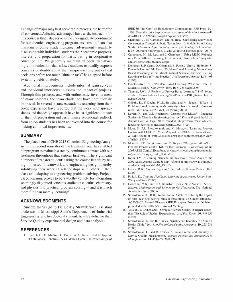
Bill Elmore is an associate professor of chemical engineering and the Interim Direc-tor for the School of Chemical Engineering at Mississippi State University. Now in his 22nd year of higher education, his focus is primarily on engineering education and the integration of problem-based learning across the curriculum.
© Copyright ChE Division of ASEE 2011
ChE curriculum
Vol. 45, No. 2, Spring 2011 87
actively involved in the same design project simultaneously (in contrast to the traditional Unit Operations laboratory ap-proach relying on the rotation of student groups through a single experimental apparatus sequentially). Coupled with the LEGO NXT® kits, we chose a series of sensors from Vernier (e.g., pH, temperature, dissolved oxygen) that interface with the robotics kits for monitoring processes and performing simple control schemes. A significant factor in choosing the LEGO NXT® robotics kits is the use of an intuitive graphical interface for programming (based on National Instruments Labview® software). This user-friendly programming in-terface removes the focus from programming and places it on the broader objectives of problem analysis and design of engineering processes.
CHE 2213 Chemical Engineering Analysis is a required, three-credit-hour course, offered once per year in the second semester of the freshman year (after a one-hour orientation and before the sophomore-level Mass & Energy Balances course). A large number of students entering the chemical engineering program at Mississippi State University (MSU) are community/junior college transfers from an extensive two-year college system throughout the state. Analysis is among the courses required for their first year at MSU. En-rollment lies typically between 55-70 students. The course is conducted in a 160-seat auditorium, the adjacent Unit Operations laboratory, and, with some design competitions, in the connecting hallway for maximum exposure to passing students from other classes.
Through loads of laughter and enthusiasm, discovery and
creativity, and precautions to avoid spending an inordinate amount of time on their robotics projects, teams of students have consistently pushed the course content forward in subse-quent semesters—demonstrating the value of a highly visual, project-based approach to learning engineering fundamentals. Through several iterations we have constructed projects more directly oriented to chemical engineering for illustrating the importance of fundamental concepts including basic units and measures, materials balances, and the fundamentals of process control.
LEARNING OBJECTIVES AND OUTCOMESTable 1 describes the learning objectives and outcomes
for the Analysis course. Defining a learning objective as a specific, targeted description of acquired knowledge or skill and a learning outcome as a broader response to particular situations requiring use of that acquired knowledge or skill, these course objectives and outcomes are being affirmed over time in coordination with our overall chemical engineering program objectives.
THE LEARNING ENVIRONMENT AND COURSE STRUCTURE
Offered Tuesdays and Thursdays for two 2-hour-and-20-minute sessions, Analysis comprises one credit hour of labora-tory and two credit hours of lecture. The learning environment is patterned after a studio setting. I provide instruction on specific topics or skills as needed in a dynamic, laboratory environment that allows students to immediately put that knowledge or skill to practice on the current project. Projects are structured to require use of accumulated knowledge over the course of the semester. Class discussions center around knowledge and skills needed for use on a timely basis. Home-work problems are assigned to allow practice of key tools. Grades come primarily from individual quizzes and the final exam (evaluating their understanding of skills and concepts learned during design exercises). Some portion of the grade is derived from team participation in oral and written reports (in varying percentages over the semesters since the course’s inception). No grade has yet been assigned for the quality or performance of designs.
Table 2 (next page) describes the flow and content for Analysis. Up to six in-class quizzes are given at appropri-ate junctures, evaluating students’ comprehension and use of the concepts, skills, and tools learned to date. Beginning with Team Challenge #2, all designs require quantitative data acquisition and analysis and are accompanied by team written reports, team self-evaluations, and oral reports.
Over the eight semesters we have offered Analysis in its cur-rent format, a surprising number of students have expressed little past experience playing with LEGOs®. To put every-one at ease at the course outset, student teams construct the LEGO® NXT robotics kits and build a mobile robot of their
TABLE 1CHE 2213 Analysis
Learning Objectives & OutcomesLearning Objectives:
At the end of this course, you should be able to…
• Brainstorm a problem quickly within a team setting (or working alone) listing a number of possible solutions over a broad range of ideas
• Describe the Engineering Design Cycle as used in this course and steps/tools involved in engineering design
• Take an idea for solving an engineering problem and bring it to a complete, functioning prototype using the LEGO NXT robotics system and accessories
• Use Microsoft Excel® tools to collect and analyze data from your engineering designs
• Describe the importance and basic elements of conducting a mate-rial balance for and maintaining control of a chemical process.
Learning Outcomes:
Upon completion of this course, you should be able to…
• Employ the Design Cycle for both originating an engineering design and for making performance improvements in an existing design
• Explain to someone in your family (a non-engineer) what chemi-cal engineering is all about—giving some very practical examples.
Chemical Engineering Education88
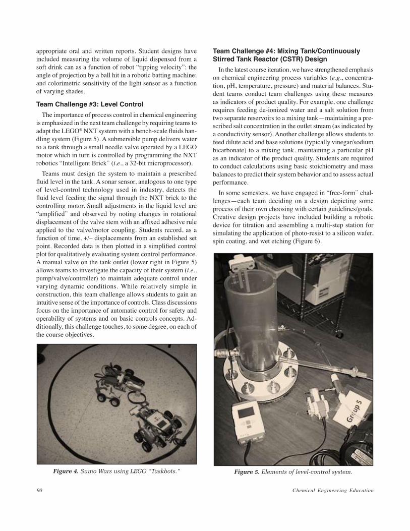
engineering design principles. Introduction of the Design Cycle (Figure 3) provides teams a guide for iteratively approaching an optimal solution for the problem they are tasked with solving.
TABLE 2Course Structure
ChE 2213 Analysis comprises approximately 28 studio sessions over 14 weeks.
• Course Orientation—one studio session (2 hrs. 20 min. per session)
a. Brainstorming
b. Using the Engineering Design Cycle
c. Data acquisition and analysis using Microsoft Excel®
d. Exploration of LEGO NXT® robotics kits
• Team Challenge #1 Taskbots & Sumo Wars—four studio sessions
a. Learning to use the LEGO NXT® system
• Team Challenge #2 Free format Design using LEGO NXT® sensors—five studio sessions
a. Teams design an experiment of their choosing using one or more of the sensors provided in the LEGO NXT® kit (i.e., rotational, pressure, light, ultrasonic, or sound sensors)
b. Constraints require clear establishment of an independent/dependent variable with elimination of extraneous parameters (where possible)
c. Brainstorming, critical thinking, teaming skills emphasized
d. Data acquisition and analysis using Microsoft’s Excel®
• Team Challenge #3 Level Control Experiment—five studio sessions
a. Interfacing the robotics kits with a tank/submersible pump/valve system assembled in-house by the student teams
b. Level control experiment
c. Explanation of fundamental control concepts
d. Level control is measured over time by control valve deflection from an established setpoint
• Team Challenge #4 Mixing tank/Continuously stirred tank reactor (CSTR) design—eight studio sessions
a. Case 1—Two feed tanks supply two separate components for mixing in a third tank (e.g., deionized water and a salt solution to be mixed to a specified salinity)
b. Case 2—Two reactant tanks supply reactants to a CSTR from which a specific product quality must be obtained (e.g., pH, coloration, dissolved oxygen level)
• Individual quizzes—five studio sessions
• Final exam
Figure 1. Students becoming familiar with the LEGO NXT® kit.
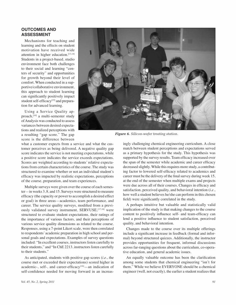
choice, using as a guide the “Taskbot” design included with the kit (Figure 1). This enables students unfamiliar with LEGO structural elements and the various sensors included in the kit to quickly learn something about the capabilities and limits of both the building components and the available sensor technology.
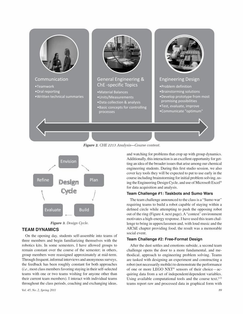
Key aspects of the course content are shown in Fig-ure 2. The Analysis course was placed in the second semester of the freshman year to engage our chemical engineering students in team-oriented, “real engineer-ing” projects at a critical stage of their collegiate (and chemical engineering) experience, thereby strengthen-ing their communication and working relationships among one another, while giving them insight into the importance of their preparatory mathematics and science courses. Students have commented on the timeliness of design projects requiring use of topics just covered in math and chemistry.
Through the introduction of increasingly complex “team challenges” students are engaged in an integra-tion of communication skills, engineering topics, and
Vol. 45, No. 2, Spring 2011 89
Communication •Teamwork •Oral reporting •Written technical summaries
General Engineering & ChE -specific Topics •Material Balances •Units/Measurements •Data collection & analysis •Basic concepts for controlling processes
Engineering Design •Problem definition •Brainstorming solutions •Develop prototype from most promising possibilities •Test, evaluate, improve •Communicate "optimum"
Figure 2. CHE 2213 Analysis—Course content.
Envision
Plan
BuildEvaluate
Refine
Figure 3. Design Cycle.
TEAM DYNAMICSOn the opening day, students self-assemble into teams of
three members and begin familiarizing themselves with the robotics kits. In some semesters, I have allowed groups to remain constant over the course of the semester; in others, group members were reassigned approximately at mid-term. Through frequent, informal interviews and anonymous surveys, the feedback has been roughly constant for both approaches (i.e., most class members favoring staying in their self-selected teams with one or two teams wishing for anyone other than their current team members). I interact with individual teams throughout the class periods, coaching and exchanging ideas,
and watching for problems that crop up with group dynamics. Additionally, this interaction is an excellent opportunity for get-ting an idea of the broader issues that arise among our chemical engineering students. During this first studio session, we also cover key tools they will be expected to put to use early in the course including brainstorming for initial problem solving, us-ing the Engineering Design Cycle, and use of Microsoft Excel® for data acquisition and analysis.Team Challenge #1: Taskbots and Sumo Wars
The team challenge announced to the class is a “Sumo war” requiring teams to build a robot capable of staying within a defined circle while attempting to push the opposing robot out of the ring (Figure 4, next page). A “contest” environment motivates a high-energy response. I have used this team chal-lenge to bring in upperclassmen and, with loud music and the AIChE chapter providing food, the result was a memorable social event.Team Challenge #2: Free-Format Design
After the dust settles and emotions subside, a second team challenge opens the door to a more fundamental, and me-thodical, approach to engineering problem solving. Teams are tasked with designing an experiment and constructing a robot (not necessarily mobile) to demonstrate the performance of one or more LEGO NXT® sensors of their choice—ac-quiring data from a set of independent/dependent variables. Using available computational tools and the course text,[12] teams report raw and processed data in graphical form with
Chemical Engineering Education90
Team Challenge #4: Mixing Tank/Continuously Stirred Tank Reactor (CSTR) Design
In the latest course iteration, we have strengthened emphasis on chemical engineering process variables (e.g., concentra-tion, pH, temperature, pressure) and material balances. Stu-dent teams conduct team challenges using these measures as indicators of product quality. For example, one challenge requires feeding de-ionized water and a salt solution from two separate reservoirs to a mixing tank—maintaining a pre-scribed salt concentration in the outlet stream (as indicated by a conductivity sensor). Another challenge allows students to feed dilute acid and base solutions (typically vinegar/sodium bicarbonate) to a mixing tank, maintaining a particular pH as an indicator of the product quality. Students are required to conduct calculations using basic stoichiometry and mass balances to predict their system behavior and to assess actual performance.
In some semesters, we have engaged in “free-form” chal-lenges—each team deciding on a design depicting some process of their own choosing with certain guidelines/goals. Creative design projects have included building a robotic device for titration and assembling a multi-step station for simulating the application of photo-resist to a silicon wafer, spin coating, and wet etching (Figure 6).
Figure 5. Elements of level-control system.
Figure 4. Sumo Wars using LEGO “Taskbots.”
appropriate oral and written reports. Student designs have included measuring the volume of liquid dispensed from a soft drink can as a function of robot “tipping velocity”; the angle of projection by a ball hit in a robotic batting machine; and colorimetric sensitivity of the light sensor as a function of varying shades.
Team Challenge #3: Level ControlThe importance of process control in chemical engineering
is emphasized in the next team challenge by requiring teams to adapt the LEGO® NXT system with a bench-scale fluids han-dling system (Figure 5). A submersible pump delivers water to a tank through a small needle valve operated by a LEGO motor which in turn is controlled by programming the NXT robotics “Intelligent Brick” (i.e., a 32-bit microprocessor).
Teams must design the system to maintain a prescribed fluid level in the tank. A sonar sensor, analogous to one type of level-control technology used in industry, detects the fluid level feeding the signal through the NXT brick to the controlling motor. Small adjustments in the liquid level are “amplified” and observed by noting changes in rotational displacement of the valve stem with an affixed adhesive rule applied to the valve/motor coupling. Students record, as a function of time, +/– displacements from an established set point. Recorded data is then plotted in a simplified control plot for qualitatively evaluating system control performance. A manual valve on the tank outlet (lower right in Figure 5) allows teams to investigate the capacity of their system (i.e., pump/valve/controller) to maintain adequate control under varying dynamic conditions. While relatively simple in construction, this team challenge allows students to gain an intuitive sense of the importance of controls. Class discussions focus on the importance of automatic control for safety and operability of systems and on basic controls concepts. Ad-ditionally, this challenge touches, to some degree, on each of the course objectives.
Vol. 45, No. 2, Spring 2011 91
OUTCOMES AND ASSESSMENT
Mechanisms for teaching and learning and the effects on student motivation have received wide attention in higher education.[13,14] Students in a project-based, studio environment face both challenges to their social and learning “cen-ters of security” and opportunities for growth beyond their level of comfort. When conducted in a sup-portive/collaborative environment, this approach to student learning can significantly positively impact student self-efficacy[15] and prepara-tion for advanced learning.
Using a Service Quality ap-proach,[16] a multi-semester study of Analysis was conducted to assess variances between desired expecta-tions and realized perceptions with a resulting “gap score.” The gap score is the difference between what a customer expects from a service and what the cus-tomer perceives as being delivered. A negative quality gap score indicates the service is not meeting expectations, while a positive score indicates the service exceeds expectations. Scores are weighted according to students’ relative expecta-tions from certain characteristics of the course. The study was structured to examine whether or not an individual student’s efficacy was impacted by realistic expectations, perceptions of the course, preparation, and team experiences.
Multiple surveys were given over the course of each semes-ter—in weeks 3, 8, and 15. Surveys were structured to measure efficacy (the capacity or power to accomplish a desired effect or goal) in three areas—academics, team performance, and career. The service quality surveys, modified from a previ-ously validated survey instrument, SERVUSE,[17,18] were structured to evaluate student expectations, their ratings of the importance of various factors, and their perceptions of various service quality dimensions as related to the course. Responses, using a 7-point Likert scale, were then correlated to respondents’ academic preparation in high school and per-sonal goals and expectations. Examples of survey questions included: “In excellent courses, instructors listen carefully to their students,” and “In ChE 2213, instructors listen carefully to their students.”
As anticipated, students with positive gap scores (i.e., the course met or exceeded their expectations) scored higher in academic-, self-, and career-efficacy[16]—an indication of self-confidence needed for moving forward in an increas-
ingly challenging chemical engineering curriculum. A close match between student perceptions and expectations served as a primary hypothesis for the study. This hypothesis was supported by the survey results. Team efficacy increased over the span of the semester while academic and career efficacy decreased slightly. While this requires more study, a contribut-ing factor to lowered self-efficacy related to academics and career must be the delivery of the final survey during week 15, at the end of the semester when multiple exams and projects were due across all of their courses. Changes in efficacy and satisfaction, perceived quality, and behavioral intention (i.e., how well a student believes he/she can perform in this chosen field) were significantly correlated in the study.
A perhaps intuitive but valuable and statistically valid implication of the study is that making changes to the course content to positively influence self- and team-efficacy can lend a positive influence to student satisfaction, perceived quality, and behavioral intention.
Changes made to the course over its multiple offerings include a significant increase in feedback (formal and infor-mal) beyond structured quizzes. Additionally, the instructor provides opportunities for frequent, informal discussions across far-ranging questions about the curriculum, co-opera-tive education, and general academic issues.
An equally valuable outcome has been the clarification among some students that chemical engineering “isn’t for them.” While we believe EVERYONE should be a chemical engineer (well, not exactly), the earlier a student realizes that
Figure 6. Silicon-wafer treating station.
Chemical Engineering Education92
a change of major may best serve their interests, the better for all concerned. A distinct advantage I have as the instructor for this course is that I also serve as the undergraduate coordinator for our chemical engineering program. As a result, I can also maintain ongoing academic/career advisement—regularly discussing with individual students their academic progress, interest, and preparation for participating in cooperative education, etc. We generally maintain an open, free-flow-ing communication that allows students to readily express concerns or doubts about their major—sorting out critical decisions before too much “time on task” has elapsed before switching fields of study.
Additional improvements include informal team surveys and individual interviews to assess the impact of projects. Through this process, and with enthusiastic inventiveness of many students, the team challenges have continuously improved. In several instances, students returning from their co-op experience have reported that the work with spread-sheets and the design approach have had a significant impact on their job preparation and performance. Additional feedback from co-op students has been re-invested into the course for making continual improvements.
SUMMARYThe placement of CHE 2213 Chemical Engineering Analy-
sis in the second semester of the freshman year has enabled our program to maintain a steady, continuous contact with our freshmen throughout that critical first year. The significant numbers of transfer students taking the course benefit by be-ing immersed in teamwork and engineering design, thereby solidifying their working relationships with others in their class and adapting to engineering problem solving. Project-based learning proves to be a worthy vehicle for integrating seemingly disjointed concepts studied in calculus, chemistry, and physics into practical problem solving— and it is much more fun than merely lecturing!
ACKNOWLEDGMENTSSincere thanks go to Dr. Lesley Strawderman, assistant
professor in Mississippi State’s Department of Industrial Engineering, and her doctoral student, Arash Salehi, for their Service Quality experimental design and data analysis.
REFERENCES 1. Lund, H.H., O. Miglino, L. Pagliarini, A. Billard, and A. Ijspeert,
“Evolutionary Robotics—A Children’s Game,” In Proceedings of
IEEE 5th Intl. Conf. on Evolutionary Computation; IEEE Press, NJ, 1998. From the link <http://citeseerx.ist.psu.edu/viewdoc/download?doi=10.1.1.35.6283&rep=rep1&type=ps> (1998)
2. Chambers, J., M. Carbonaro, and M. Rex, “Scaffolding Knowledge Construction Through Robotic Technology: A Middle School Case Study,” Electronic J. for the Integration of Technology in Education, 6, 55–70. From <http://ejite.isu.edu/Volume6/Chambers.pdf> (2007)
3. Carbonaro, M., M. Rex, and J. Chambers, “Using LEGO Robotics in a Project-Based Learning Environment,” from <http://imej.wfu.edu/articles/2004/1/02/index.asp>
4. Kolodner, J., P. Camp, D. Crismond, B. Fasse, J. Gray, J. Holbrook, S. Puntambekar, and M. Ryan, “Problem-Based Learning Meets Case-Based Reasoning in the Middle-School Science Classrom: Putting Learning by DesignTM into Practice,” J. of Learning Sciences, 12(4) 495 (2003)
5. Hmelo-Silver, C.E., “Problem-Based Learning: What and How Do Students Learn?,” Edu. Psych. Rev., 16(3) 235 (Sept. 2004)
6. Thomas, J.W., “A Review of Project-Based Learning,” 1-45, found at <http://www.bobpearlman.org/BestPractices/PBL_Research.pdf> (March 2000)
7. Gijbels, D., F. Dochy, P.V.D. Bossche, and M. Segers, “Effects of Problem-Based Learning: A Meta-Analysis from the Angle of Assess-ment,” Rev. Edu. Rsrch., 75(1) 27 (Spring 2005)
8. Levien, K., and W.E. Rochefort, “Lessons with LEGO®—Engaging Students in Chemical Engineering Courses,” Proceedings of the ASEE Annual Conf. & Exp., 2002; found at <http://www.rowan.edu/col-leges/engineering/clinics/asee/papers/2002/1672>
9. Moor, S., P.R. Piergiovanni, and M. Metzger, “Learning Process Control with LEGOs®,” Proceedings of the 2004 ASEE Annual Conf. & Exp.; found at <http://soa.asee.org/paper/conference/paper-view.cfm?id=19879>
10. Moor, S., P.R. Piergiovanni, and D. Keyser, “Design—Build—Test: Flexible Process Control Kits for the Classroom,” Proceedings of the 2003 ASEE Conf. & Exp; found at <http://www.ni.com/pdf/academic/us/journals/Design_Build_Test.pdf>
11. Keith, J.M., “Learning “Outside the Toy Box,” Proceedings of the 2002 ASEE Annual Conf. & Exp.; <found at http://www.ni.com/pdf/academic/us/journals/lv02_43.pdf>
12. Larsen, R.W., Engineering with Excel, 3rd ed., Pearson Prentice Hall (2009)
13. Fink, L.D., Creating Significant Learning Experiences, Jossey-Bass, Wiley and Sons (2003)
14. Donovan, M.S., and J.D. Bransford (eds.), How Students Learn: History, Mathematics and Science in the Classroom, The National Academies Press (2005)
15. Strawderman, L., B.B. Elmore, and A. Aslehi, “Exploring the Impact of First-Year Engineering Student Perceptions on Student Efficacy,” AC2009-62; Second Place—ASEE First-year Programs Division; presented at the 2009 ASEE Annual Meeting
16. Voss, R., T. Gruber, and I. Szmigin, “Service Quality in Higher Educa-tion: The Role of Student Expectations,” J. of Bus. Rsrch., 60; 949-959 (2007)
17. Strawderman, L., and R. Koubek, “Quality and Usability in a Student Health Clinic,” Intl. J. of Health Care Quality Assurance, 19, 225-236 (2006)
18. Strawderman, L., and R. Koubek, “Human Factors and Usability in Service Quality Measurement,” Human Factors and Ergonomics in Manufacturing, 18, 454-463 (2008) p
Vol. 45, No. 2, Spring 2011 93
Fluid viscosity is an important fluid property to monitor in industry, research, and medicine. The diverse ap-plications for the rapid measurement of fluid viscosity
include the characterization of inks in ink-jet printing, [1] stud-ies of protein dynamics,[2] the characterization of biomaterials used in drug delivery such as hyaluronic acid (HA), [3] and the clinical detection of diseases such as paraproteinemia[4] and ischemic heart disease[5] through the study of blood. An additional use of viscometry is in the determination of the hydrodynamic volume and molecular weight of macro-molecules. Using the data analysis seen later in this paper, a polymer’s molecular weight can be estimated. It is important to be able to measure a polymer’s molecular weight—because of its impact on such properties as strength, stiffness, and glass transition temperature—by simply measuring the viscosity of dilute polymer solutions of varying concentrations.
In a laboratory setting, viscosity measurements of dilute polymer solutions are typically made with glass capillary viscometers such as Ubbelohde viscometers that require mL of fluid for measurement. The development of microfluidic viscometers[6-9] means that such viscosity measurements can now be quickly made with only μL of fluid. Microviscom-eters can thus potentially be used to determine the molecular weight of polymer samples even when sample volumes are severely limited.
To illustrate both the use of microfluidics to determine fluid viscosity and the use of dilute solution viscometry to determine polymer molecular weight, we developed a low-cost laboratory procedure for students to use PDMS micro-viscometers to determine the molecular weight of a polymer sample. In addition to the procedure, we present sample data for microviscometer tests run on glycerol solutions and on
samples of PEO that match up well with viscometry results obtained with conventional Ubbelohde viscometers. We also discuss the timing and logistics of the lab and the feedback obtained from two sample laboratory sessions run with un-dergraduates.
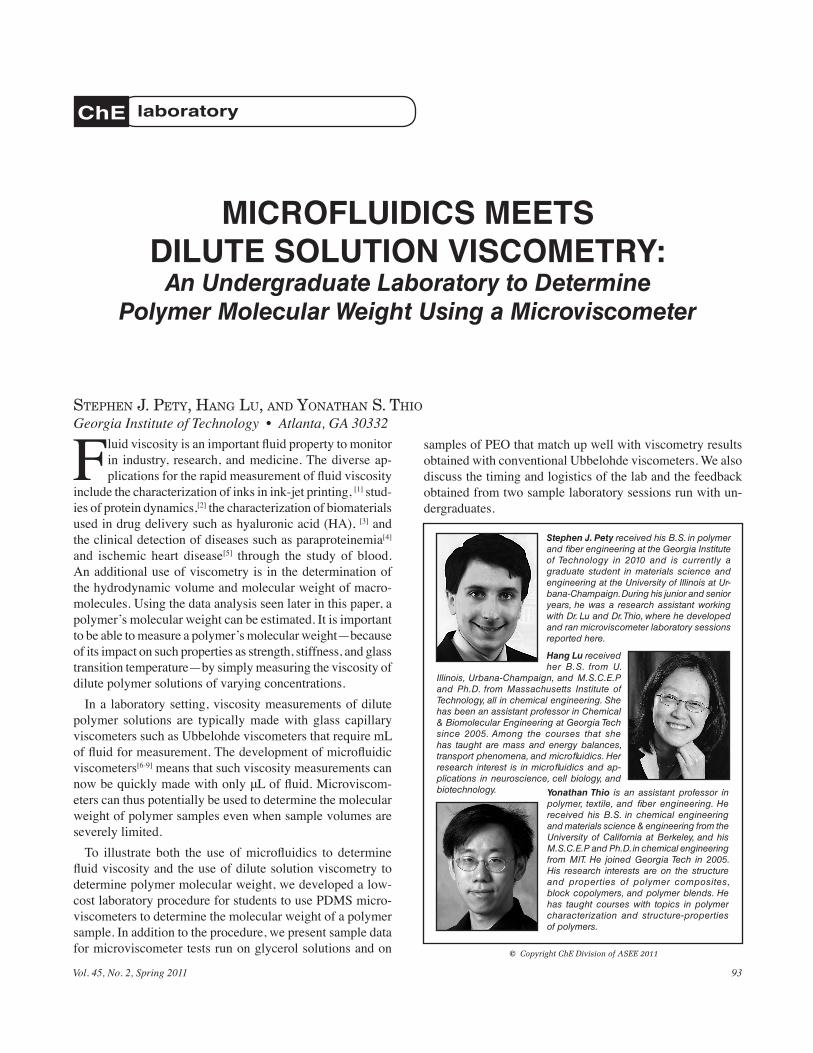
Stephen J. Pety received his B.S. in polymer and fiber engineering at the Georgia Institute of Technology in 2010 and is currently a graduate student in materials science and engineering at the University of Illinois at Ur-bana-Champaign. During his junior and senior years, he was a research assistant working with Dr. Lu and Dr. Thio, where he developed and ran microviscometer laboratory sessions reported here.
Yonathan Thio is an assistant professor in polymer, textile, and fiber engineering. He received his B.S. in chemical engineering and materials science & engineering from the University of California at Berkeley, and his M.S.C.E.P and Ph.D. in chemical engineering from MIT. He joined Georgia Tech in 2005. His research interests are on the structure and properties of polymer composites, block copolymers, and polymer blends. He has taught courses with topics in polymer characterization and structure-properties of polymers.
Hang Lu received her B.S. from U.
Illinois, Urbana-Champaign, and M.S.C.E.P and Ph.D. from Massachusetts Institute of Technology, all in chemical engineering. She has been an assistant professor in Chemical & Biomolecular Engineering at Georgia Tech since 2005. Among the courses that she has taught are mass and energy balances, transport phenomena, and microfluidics. Her research interest is in microfluidics and ap-plications in neuroscience, cell biology, and biotechnology.
© Copyright ChE Division of ASEE 2011
MICROFLUIDICS MEETS DILUTE SOLUTION VISCOMETRY:
An Undergraduate Laboratory to Determine Polymer Molecular Weight Using a Microviscometer
ChE laboratory
StEphEn J. pEty, hang lu, and yonathan S. thio
Georgia Institute of Technology • Atlanta, GA 30332
Chemical Engineering Education94
MATERIALSFor soft lithography microchannel fabrication, SU-
8 2050 negative photoresist and SU-8 developer were acquired from Microchem (Newton, MA). Sylard-184 poly(dimethylsiloxane) (PDMS) was obtained from Dow Corning (Midland, MI) and 1,1,2-trichlorosilane (T2492) (a release agent) was obtained from United Chemical Technolo-gies (Bristol, PA). Samples of PEO with viscosity average molecular weights of ~1 MDa and ~4 MDa were obtained from Sigma-Aldrich (St. Louis, MO). Aqueous solutions of the 1 MDa PEO were prepared by mixing the solutions with a stir bar overnight. Experiments to determine the viscosity of these solutions were performed within eight days of when the
solutions were prepared. An aqueous solution of 3 mg/mL of the 4 MDa was prepared by stirring the solution for three days. The shear thinning studies performed using this solution were performed within one day of when the solution was prepared. Glycerol from Fisher Scientific (Pittsburgh, PA) was used to prepare aqueous glycerol solutions.
METHODSDevice Fabrication
Microfluidic viscometers (PDMS channel on PDMS flat substrate) were fabricated using the rapid prototyping tech-nique.[10] Briefly, the viscometer device was designed using AutoCAD (Autodesk, San Rafael, CA). A silicon-SU-8 master
was created using conven-tional UV photolithography (with the SU-8 layer being 55 μm). After surface treatment of gas-phase 1,1,2-trichlo-rosilane (a release agent) on the master, a degassed 10:1 mixture of PDMS precursor and curing agent was then cast onto the master (about 2.5 mm thick—thickness not critical). After being cured at 70 ˚C for at least two hours, the PDMS slab was peeled from the master and cut into devices. A flat PDMS slab and the PDMS piece with the chan-nel imprints were then treated for 30 seconds in an air plasma (Harrick Plasma, Ithaca, NY)
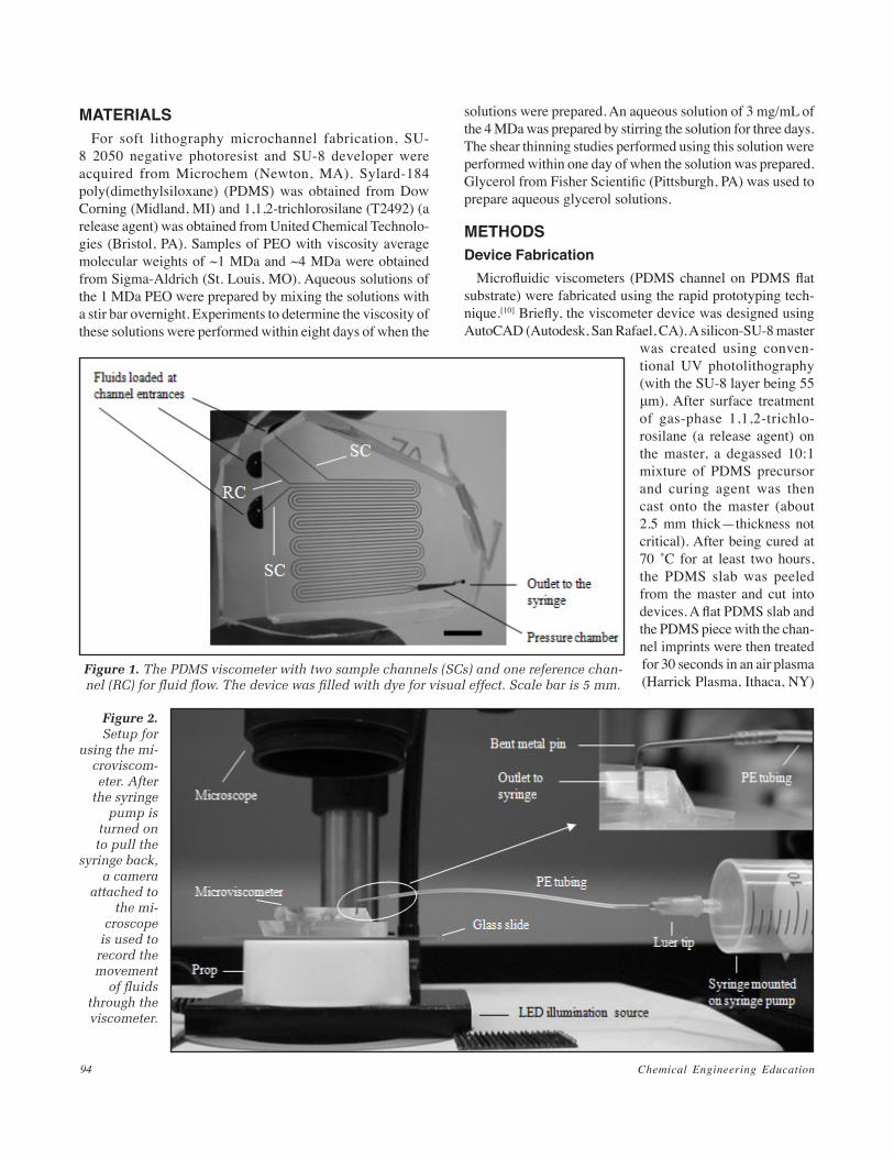
Figure 1. The PDMS viscometer with two sample channels (SCs) and one reference chan-nel (RC) for fluid flow. The device was filled with dye for visual effect. Scale bar is 5 mm.
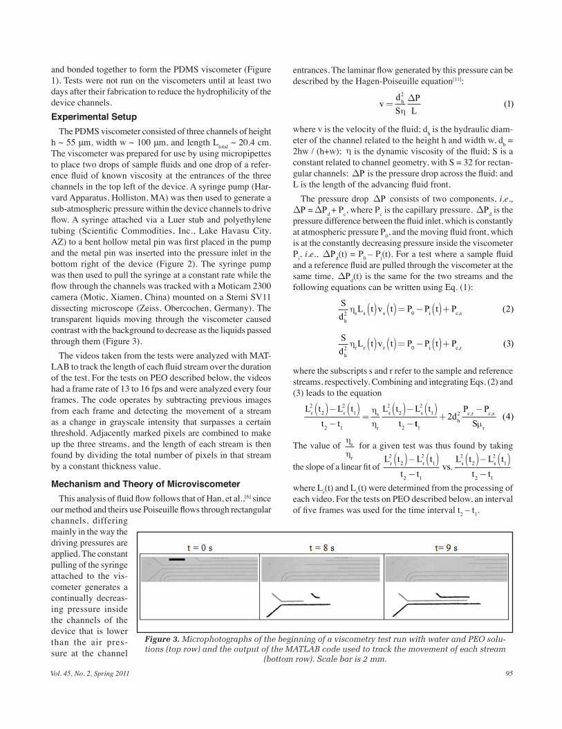
Figure 2. Setup for
using the mi-croviscom-eter. After
the syringe pump is
turned on to pull the
syringe back, a camera
attached to the mi-
croscope is used to
record the movement
of fluids through the viscometer.
Vol. 45, No. 2, Spring 2011 95
and bonded together to form the PDMS viscometer (Figure 1). Tests were not run on the viscometers until at least two days after their fabrication to reduce the hydrophilicity of the device channels.Experimental Setup
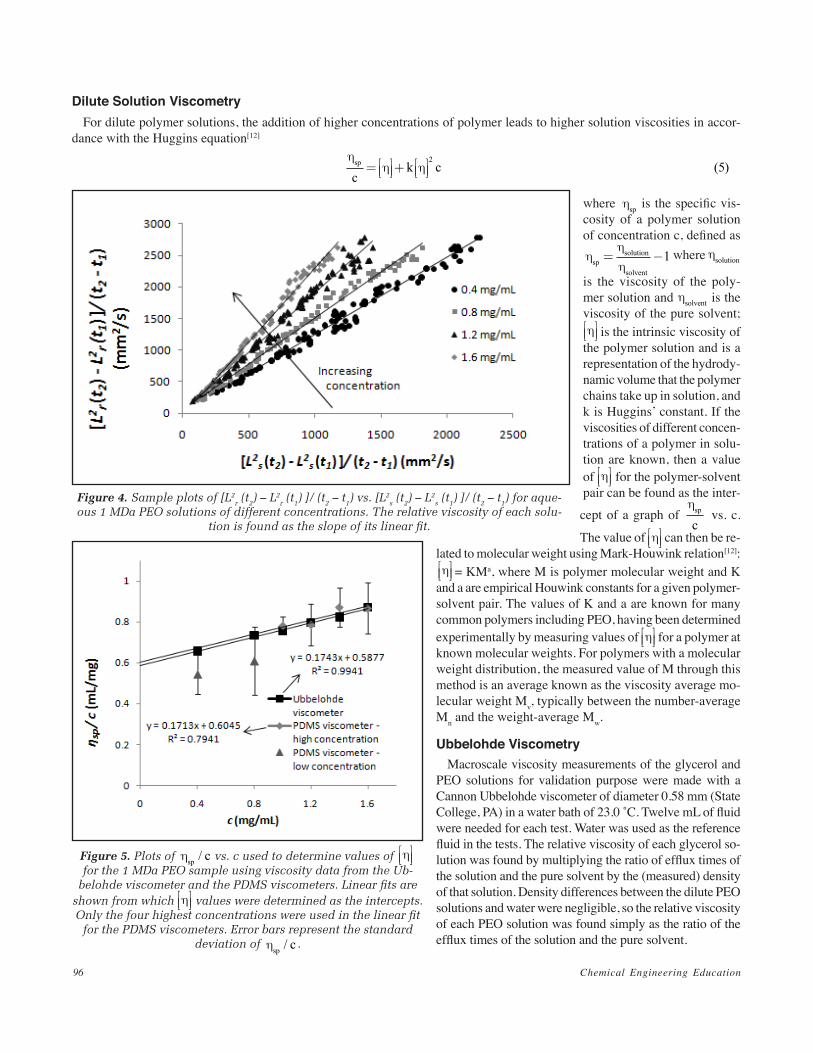
The PDMS viscometer consisted of three channels of height h ~ 55 μm, width w ~ 100 μm, and length Ltotal ~ 20.4 cm. The viscometer was prepared for use by using micropipettes to place two drops of sample fluids and one drop of a refer-ence fluid of known viscosity at the entrances of the three channels in the top left of the device. A syringe pump (Har-vard Apparatus, Holliston, MA) was then used to generate a sub-atmospheric pressure within the device channels to drive flow. A syringe attached via a Luer stub and polyethylene tubing (Scientific Commodities, Inc., Lake Havasu City, AZ) to a bent hollow metal pin was first placed in the pump and the metal pin was inserted into the pressure inlet in the bottom right of the device (Figure 2). The syringe pump was then used to pull the syringe at a constant rate while the flow through the channels was tracked with a Moticam 2300 camera (Motic, Xiamen, China) mounted on a Stemi SV11 dissecting microscope (Zeiss, Obercochen, Germany). The transparent liquids moving through the viscometer caused contrast with the background to decrease as the liquids passed through them (Figure 3).
The videos taken from the tests were analyzed with MAT-LAB to track the length of each fluid stream over the duration of the test. For the tests on PEO described below, the videos had a frame rate of 13 to 16 fps and were analyzed every four frames. The code operates by subtracting previous images from each frame and detecting the movement of a stream as a change in grayscale intensity that surpasses a certain threshold. Adjacently marked pixels are combined to make up the three streams, and the length of each stream is then found by dividing the total number of pixels in that stream by a constant thickness value.
Mechanism and Theory of MicroviscometerThis analysis of fluid flow follows that of Han, et al.,[6] since
our method and theirs use Poiseuille flows through rectangular channels, differing mainly in the way the driving pressures are applied. The constant pulling of the syringe attached to the vis-cometer generates a continually decreas-ing pressure inside the channels of the device that is lower than the air pres-sure at the channel
entrances. The laminar flow generated by this pressure can be described by the Hagen-Poiseuille equation[11]:
vdS
PL
h=∆2 1η
( )
where v is the velocity of the fluid; dh is the hydraulic diam-eter of the channel related to the height h and width w, dh = 2hw / (h+w); η is the dynamic viscosity of the fluid; S is a constant related to channel geometry, with S = 32 for rectan-gular channels; ∆P is the pressure drop across the fluid; and L is the length of the advancing fluid front.
The pressure drop ∆P consists of two components, i.e., ∆P =∆Pd + Pc, where Pc is the capillary pressure. ∆Pd is the pressure difference between the fluid inlet, which is constantly at atmospheric pressure P0, and the moving fluid front, which is at the constantly decreasing pressure inside the viscometer Pi, i.e., ∆Pd(t) = P0 – Pi(t). For a test where a sample fluid and a reference fluid are pulled through the viscometer at the same time, ∆Pd(t) is the same for the two streams and the following equations can be written using Eq. (1):
Sd
L t v t P P t Ph
s s s i c s2 0 2η ( ) ( )= − ( )+ , ( )
Sd
L t v t P P t Ph
r r r i c r2 0 3η ( ) ( )= − ( )+ , ( )
where the subscripts s and r refer to the sample and reference streams, respectively. Combining and integrating Eqs. (2) and (3) leads to the equation
L t L tt t
L t L tt
r r s
r
s s2
22
1
2 1
22
21
2
( )− ( )−
=( )− ( )−
ηη tt
dP PSh
c r c s
r1
22 4+−, , ( )µ
The value of ηηs
r
for a given test was thus found by taking
the slope of a linear fit of L t L t
t tvsL t L t
t tr r s s2
22
1
2 1
22
21
2 1
( )− ( )−
( )− ( )−
.
where Lr(t) and Ls(t) were determined from the processing of each video. For the tests on PEO described below, an interval of five frames was used for the time interval t2 – t1.
Figure 3. Microphotographs of the beginning of a viscometry test run with water and PEO solu-tions (top row) and the output of the MATLAB code used to track the movement of each stream
(bottom row). Scale bar is 2 mm.
Chemical Engineering Education96
Dilute Solution ViscometryFor dilute polymer solutions, the addition of higher concentrations of polymer leads to higher solution viscosities in accor-
dance with the Huggins equation[12]
ηη ηsp
ck c=
+2
5( )
where ηsp is the specific vis-cosity of a polymer solution of concentration c, defined as η
ηηsp
solution
solvent
= −1 where ηsolution
is the viscosity of the poly-mer solution and ηsolvent is the viscosity of the pure solvent; η is the intrinsic viscosity of
the polymer solution and is a representation of the hydrody-namic volume that the polymer chains take up in solution, and k is Huggins’ constant. If the viscosities of different concen-trations of a polymer in solu-tion are known, then a value of η for the polymer-solvent
pair can be found as the inter-
cept of a graph of ηspc
vs. c.
The value of η can then be re-
lated to molecular weight using Mark-Houwink relation[12]: η = KMa, where M is polymer molecular weight and K
and a are empirical Houwink constants for a given polymer-solvent pair. The values of K and a are known for many common polymers including PEO, having been determined experimentally by measuring values of η
for a polymer at
known molecular weights. For polymers with a molecular weight distribution, the measured value of M through this method is an average known as the viscosity average mo-lecular weight Mv, typically between the number-average Mn and the weight-average Mw.
Ubbelohde ViscometryMacroscale viscosity measurements of the glycerol and
PEO solutions for validation purpose were made with a Cannon Ubbelohde viscometer of diameter 0.58 mm (State College, PA) in a water bath of 23.0 ̊ C. Twelve mL of fluid were needed for each test. Water was used as the reference fluid in the tests. The relative viscosity of each glycerol so-lution was found by multiplying the ratio of efflux times of the solution and the pure solvent by the (measured) density of that solution. Density differences between the dilute PEO solutions and water were negligible, so the relative viscosity of each PEO solution was found simply as the ratio of the efflux times of the solution and the pure solvent.
Figure 4. Sample plots of [L2r (t2) – L2
r (t1) ]/ (t2 – t1) vs. [L2s (t2) – L2
s (t1) ]/ (t2 – t1) for aque-ous 1 MDa PEO solutions of different concentrations. The relative viscosity of each solu-
tion is found as the slope of its linear fit.
Figure 5. Plots of ηsp c/ vs. c used to determine values of η
for the 1 MDa PEO sample using viscosity data from the Ub-belohde viscometer and the PDMS viscometers. Linear fits are
shown from which η values were determined as the intercepts.
Only the four highest concentrations were used in the linear fit for the PDMS viscometers. Error bars represent the standard
deviation of ηsp c/ .
Vol. 45, No. 2, Spring 2011 97
VALIDATION OF THE DEVICE OPERATIONTo ensure that the microviscometer produced accurate vis-
cosity readings, tests were first run on the device using glyc-erol solutions as sample streams and water as the reference stream. Pressure was generated with a 50 mL syringe that was pulled at rates ranging from 3.50 mL/min to 21.84 mL/min. Tests were performed at room temperature averaging ~ 23 ̊ C. The viscosities of the glycerol solutions were measured with an Ubbelohde viscometer in a 23.0 ˚C bath for comparison (Table 1). The results from the microviscometer are seen to be consistent with the Ubbelohde viscometer although the variance in the microviscometer tests is much higher.
Viscosity measurements were then made with the microvis-cometer using dilute 1 MDa PEO solutions as sample streams and water as the reference stream. For these tests, pressure was generated by pulling a 50 mL syringe at an initial vol-ume of 25 mL at a rate of 5.46 mL/min. Note that the exact initial volume of the syringe and the pulling rate used in the experiments are not critical, as the viscometer can function over a range of generated pressure gradients. Pressure-induced deformation of the microchannels could occur in a PDMS device such as ours if pressure differences were too large but the maximum pressure gradients across the channels in these experiments were only ~15 kPa for the glycerol tests and ~10 kPa for the PEO tests. No deformation of the channels was observed under the microscope in any test.
The PEO tests were performed at 23.0 ̊ C + 0.5 ̊ C and the mea-sured viscosity values were compared to values obtained with an Ubbelohde viscometer in a 23.0 ̊ C bath (Table 1). Sample plots of
L t L tt t
vsL t L t
t tr r s s2
22
1
2 1
22
21
2 1
( )− ( )−
( )− ( )−
.
used to calculate viscosity values in the microviscometer tests are seen in Figure 4.
In a few of the microviscometer tests, PEO solutions began to flow through the viscometer before the syringe was pulled, suggest-ing that the PEO solutions had a positive value of Pc, sample, i.e., they wet the PDMS surface. This did not interfere with data collection, however, and the results from the viscometer were still valid for times while all fluids were moving.
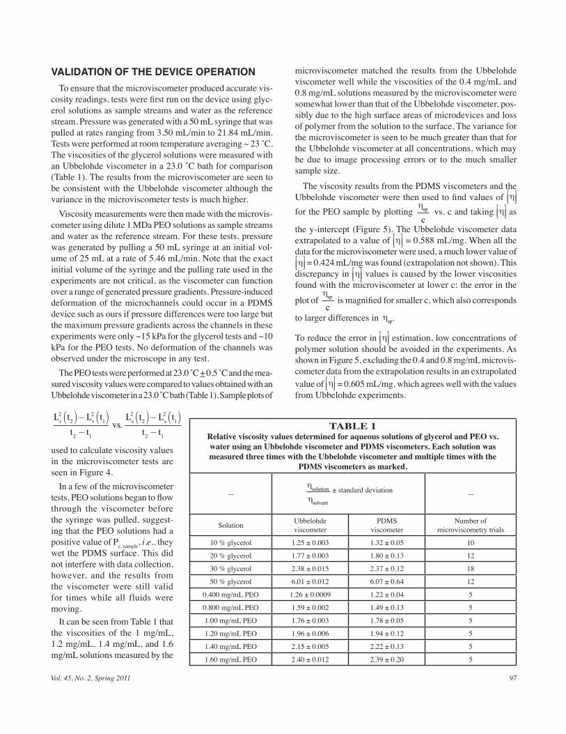
It can be seen from Table 1 that the viscosities of the 1 mg/mL, 1.2 mg/mL, 1.4 mg/mL, and 1.6 mg/mL solutions measured by the
TABLE 1Relative viscosity values determined for aqueous solutions of glycerol and PEO vs. water using an Ubbelohde viscometer and PDMS viscometers. Each solution was measured three times with the Ubbelohde viscometer and multiple times with the
PDMS viscometers as marked.
—ηη
solution
solvent
± standard deviation —
Solution Ubbelohdeviscometer
PDMSviscometer
Number ofmicroviscometry trials
10 % glycerol 1.25 ± 0.003 1.32 ± 0.05 10
20 % glycerol 1.77 ± 0.003 1.80 ± 0.13 12
30 % glycerol 2.38 ± 0.015 2.37 ± 0.12 18
50 % glycerol 6.01 ± 0.012 6.07 ± 0.64 12
0.400 mg/mL PEO 1.26 ± 0.0009 1.22 ± 0.04 5
0.800 mg/mL PEO 1.59 ± 0.002 1.49 ± 0.13 5
1.00 mg/mL PEO 1.76 ± 0.003 1.78 ± 0.05 5
1.20 mg/mL PEO 1.96 ± 0.006 1.94 ± 0.12 5
1.40 mg/mL PEO 2.15 ± 0.005 2.22 ± 0.13 5
1.60 mg/mL PEO 2.40 ± 0.012 2.39 ± 0.20 5
microviscometer matched the results from the Ubbelohde viscometer well while the viscosities of the 0.4 mg/mL and 0.8 mg/mL solutions measured by the microviscometer were somewhat lower than that of the Ubbelohde viscometer, pos-sibly due to the high surface areas of microdevices and loss of polymer from the solution to the surface. The variance for the microviscometer is seen to be much greater than that for the Ubbelohde viscometer at all concentrations, which may be due to image processing errors or to the much smaller sample size.
The viscosity results from the PDMS viscometers and the Ubbelohde viscometer were then used to find values of η
for the PEO sample by plotting ηspc
vs. c and taking η as
the y-intercept (Figure 5). The Ubbelohde viscometer data extrapolated to a value of η
= 0.588 mL/mg. When all the
data for the microviscometer were used, a much lower value of η = 0.424 mL/mg was found (extrapolation not shown). This
discrepancy in η values is caused by the lower viscosities
found with the microviscometer at lower c: the error in the
plot of ηspc
is magnified for smaller c, which also corresponds
to larger differences in ηsp.
To reduce the error in η estimation, low concentrations of
polymer solution should be avoided in the experiments. As shown in Figure 5, excluding the 0.4 and 0.8 mg/mL microvis-cometer data from the extrapolation results in an extrapolated value of η
= 0.605 mL/mg, which agrees well with the values
from Ubbelohde experiments.
Chemical Engineering Education98
Using values of a = 0.78 and K = 12.5 * 10-6 mL/mg (g/mol)1/a for aqueous PEO solutions[13] and the η
values
above, the Mark-Houwink equation produces values of M = 1,010,000 g/mol for the PDMS viscometers and M = 977,000 g/mol for the Ubbelohde viscometers. These values are in good agreement with each other as well as with the value reported by the manufacturer.
LABORATORY IMPLEMENTATION, COST AND LOGISTICS, AND STUDENT FEEDBACKLaboratory Implementation
The laboratory procedure consists of a device fabrication demonstration, student-run microviscometer tests on PEO solutions, image processing of the tests using MATLAB, and a shear-thinning demonstration. After the lab session, viscosity data from different students can be combined and analyzed to find an estimate for the molecular weight of the PEO sample used. If time is available, students can also measure the vis-cosities of the PEO solutions with macro viscometers such as Ubbelohde viscometers to validate the microviscometer data. This allows students to visualize the advantages and disad-vantages of microviscometry in terms of accuracy, precision, speed, cost, and fluid volume required.
Two trials of this procedure were run with volunteer under-graduates (mostly junior students who have taken transport
phenomena) from the Georgia Institute of Technology School of Chemical & Biomolecular Engineering. Each trial had four students with no microfluidics experience who performed the viscometer tests and the first trial had an additional three students who had worked in a microfluidics laboratory before. Several days before the laboratory sessions were held, students were provided with a copy of the procedure as well as a “pre-lab” that provided the background, theory, and a quiz to test their understanding prior to the lab. The beginning of the labora-tory consisted of a microviscometer fabrication demonstration given by the undergraduate teaching assistant. The assistant explained how masks and masters are manufactured, explained how PDMS is mixed, cast, cured, and bonded to form devices, and used the plasma cleaner to bond a device to show to the stu-dents. If time allows, this simple micromolding step and device fabrication can be incorporated into the lab, and concepts such as cross-linking, Poisson ratio, Young’s modulus, and surface treatment can be explained and demonstrated.
The students then ran two microviscometer tests where each test used two different concentrations of 1 MDa PEO as sample streams and water as the reference stream. Con-centrations of 0.500, 1.00, 1.50, and 2.00 mg/mL were used in the two tests. Pressure was generated by pulling a 50 mL syringe at an initial volume of 25 mL at a rate of 5.46 mL/min (the same conditions as in the validation tests for the PEO solutions).
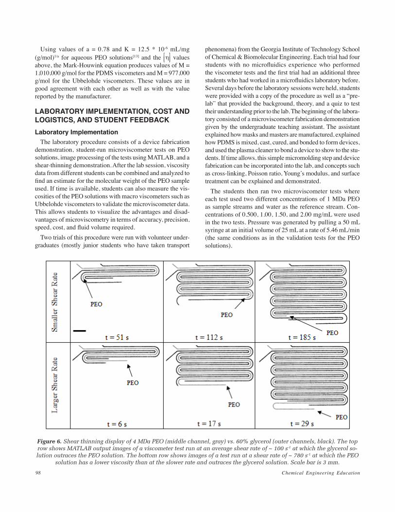
Figure 6. Shear thinning display of 4 MDa PEO (middle channel, gray) vs. 60% glycerol (outer channels, black). The top row shows MATLAB output images of a viscometer test run at an average shear rate of ~ 100 s-1 at which the glycerol so-lution outraces the PEO solution. The bottom row shows images of a test run at a shear rate of ~ 780 s-1 at which the PEO
solution has a lower viscosity than at the slower rate and outraces the glycerol solution. Scale bar is 3 mm.
Vol. 45, No. 2, Spring 2011 99
Image ProcessingThe students then used the pre-written MATLAB code to
analyze their videos. In our experience, some of the trouble-shooting issues with the image processing can be explained to the students during the lab module to facilitate data process-ing. For instance, it is important to take a video that has both high contrast (for the streams to be located by the code) and uniform contrast (for the streams to be tracked with uniform width). Problems with noisy images can be addressed with MATLAB filtering of the raw video and with data smoothing of the acquired length values.
Demonstration of Shear Thinning FluidsTo demonstrate both the shear thinning behavior of non-
dilute polymer solutions and the ability to generate a large range of shear rates in the viscometer using the syringe pump, the students then ran a test with a high pulling rate and a test with a low pulling rate on a sample of 3 mg/mL 4 MDa PEO with 60% glycerol solutions as reference fluids. When a test is run with a syringe initial volume of 40 mL and a pulling rate of 1.7 mL/min, corresponding to an average shear rate ~100 s-1, the 60% glycerol reference is seen to move through the viscometer more quickly than the PEO solution (Figure 6). In contrast, the PEO solution is seen to move through the viscometer more quickly than the 60% glycerol reference when given a higher average shear rate of ~780 s-1 (generated by pulling a syringe at an initial volume of 5 mL at a rate of 20 mL/min). This inversion of behavior is caused by the lower viscosity of the PEO solution at a higher shear rate as opposed to the rate-independent viscosity of the Newtonian glycerol solution. The shear thinning behavior of the PEO solution over this range of shear rates was verified using a Physica MCR 3000 rheometer (Anton-Paar, Graz, Austria); the viscosity of the PEO solution fell from ~ 14 cP at 100 s-1 to ~ 8.6 cP at 780 s-1. This method can be used to demonstrate non-Newtonian behaviors of various fluids in the range of shear rates up to 2000 s-1.
Cost Estimate and Timing LogisticsAssuming that laboratory equipment such as microscopes,
cameras, a plasma cleaner, and a syringe pump are available, the laboratory costs come in the materials. The fabrication of a mask and master costs around $150, and samples of the 1 MDa PEO, 4 MDa PEO, glycerol, and PDMS cost ~$30 each for a total startup cost of <$300. Note that other water-soluble poly-mers can be substituted for PEO if desired, and fluids other than glycerol solutions can be used as viscosity standards as long as they do not swell PDMS and their viscosity is known. If needed, we estimate that a simple microscope and camera setup are in the range of $2,000 to $3,000. If a plasma cleaner is not available, it is possible to create devices by pressing a flat PDMS slab against a PDMS slab with channel imprints, placing the slabs between two glass slides, and then holding the glass slides together using rubber bands.
Once the startup materials are present, the individual lab sessions have a very low cost because of the small volumes of chemicals needed. The major repeated cost is in fabricating the PDMS devices which consume ~$1.50 of PDMS per chip. Approximately 5 hours of time were devoted by the under-graduate teaching assistant to prepare for each lab session, including device fabrication, solution preparation, and lab set-up. The two lab sessions took about 1 hour and 45 minutes each to complete, including the fabrication demonstration, the completion of four viscometer tests, and the processing of the tests and the description of the MATLAB code.
Student FeedbackStudents who participated in the laboratory experiments
provided informal feedback. Most students found the mod-ule was effective in introducing the concept of solution viscometry and microfluidics, to which most of them had had no prior exposure. The students found more background on microfluidics and microfabrication details would be both more interesting and more useful. This suggests that the laboratory module should be expanded to multiple sessions to deal with the individual topics in depth. The students also commented that seeing non-Newtonian behavior with a real demonstration could reinforce this concept that they learned in the classroom.
CONCLUSIONSWe present a procedure for a student laboratory session to
demonstrate the use of microfluidics to determine fluid viscosity and the use of dilute solution viscometry to estimate polymer molecular weight. Overall, the results were reasonably consis-tent with those found from conventional Ubbelohde viscometry. The laboratory also allows students to see firsthand how micro-fluidic devices are fabricated and to observe a visual demon-stration of the shear thinning behavior of non-dilute polymer solutions. Assuming soft lithography equipment is available, the experimental setup is very quick and affordable. The laboratory serves as an excellent way to generate interest in the fields of polymers, rheology, and image processing while invigorating students with the opportunity to work hands-on in the “cutting-edge” realm of microfluidics.[14] The combination of written instruction in the pre-lab and procedure, verbal instruction and visual displays from the teaching assistant, and hands-on experience for each student caters to a range of different student learning styles.[15-16] Because it is multi-faceted, this experimen-tal platform can be used and re-used in different pedagogical contexts, or it can be a problem-solving based learning tool.[17]
We recommend running the following laboratory modules individually or in combination depending on the need of the curricula and time available for the laboratory experiments: (1) laminar flow – Hagen-Poiseuille relationship; (2) viscometry; (3) demonstration of non-Newtonian flow; (4) microfabrica-tion; (5) other concepts of polymer processing; (6) image processing.
Chemical Engineering Education100
ACKNOWLEDGMENTSWe thank M. Li for developing the microviscometer design
and the first round of MATLAB code for image processing, J. Stirman and M. Crane for their help with the microscope setup and image processing, and Dr. V. Breedveld and E. Peterson for use of their facilities.
REFERENCES 1. Calvert, P., “Inkjet Printing for Materials and Devices,” Chemistry of
Materials, 13(10) 3299 (2001) 2. Ansari, A., C.M. Jones, E.R. Henry, J. Hofrichter, and W.A. Eaton, “The
Role of Solvent Viscosity in the Dynamics of Protein Conformational Changes,” Science, 256(5065) 1796 (1992)
3. Liao, Y.-H., S.A. Jones, B. Forbes, G.P. Martin, and M.B. Brown, “Hyaluronan: Pharmaceutical Characterization and Drug Delivery,” Drug Delivery, 12(6) 327 (2005)
4. McGrath, M.A., and R. Penny, “Paraproteinemia—Blood Hyperviscos-ity and Clinical Manifestations,” J. Clin. Invest., 58(5) 1155 (1976)
5. Yarnell, J.W.G., et al., “Fibrinogen, Viscosity, and White Blood Cell Count are Major Risk Factors for Ischemic Heart Disease—The Caer-philly and Speedwell Collaborative Heart Disease Studies,” Circula-tion, 83(3) 836 (1991)
6. Han, Z., X. Tang, and B. Zheng, “A PDMS Viscometer for Microliter Newtonian Fluid,” J. Micromechanics and Microengineering, 17(9) 1828 (2007)
7. Srivastava, N., R.D. Davenport, and M.A. Burns, “Nanoliter Viscometer
for Analyzing Blood Plasma and Other Liquid Samples,” Analytical Chemistry, 77(2) 383 (2005)
8. Marinakis, G.N., J.C. Barbenel, A.C. Fisher, and S.G. Tsangaris, “A New Capillary Viscometer for Whole Blood Viscosimetry,” Biorheol-ogy, 36(4) 311 (1999)
9. Han, Z., and B. Zheng, “A PDMS Viscometer for Microliter Power Law Fluids,” J. Micromechanics and Microengineering, 19(11) 115005 (2009)
10. Duffy, D.C., J.C. McDonald, O.J.A. Schueller, and G.M. Whitesides, “Rapid Prototyping of Microfluidic Systems in Poly(dimethylsiloxane),” Analytical Chemistry, 70(23) 4974 (1998)
11. Perry, R.H., and D.W. Green, Perry’s Chemical Engineers’ Handbook, 8th Ed., McGraw-Hill, New York (2008)
12. Painter, P.C., and M.M. Coleman, Essentials of Polymer Science and Engineering, 1st Ed., DEStech Publications, Inc., Lancaster, PA (2008)
13. Bailey, F.E., and J.V. Koleske, Poly(ethylene oxide), Academic Press, New York (1976)
14. Young, E.W.K., and C.A. Simmons, “ ‘Student-Lab-on-a-Chip’: In-tegrating Low-Cost Microfluidics Into Undergraduate Teaching Labs to Study Multiphase Flow Phenomena in Small Vessels,” Chem. Eng. Ed., 43(3) 232 (2009)
15. Felder, R.M., and L.K. Silverman, “Learning and Teaching Styles in Engineering Education,” Eng. Ed., 78(7) 674 (1988)
16. Montgomery, S.M., and L.N. Groat, “Student Learning Styles and Their Implications for Teaching,” CRLT Occasional Papers, 10 (1998)
17. Major, C.H., and B. Palmer, “Assessing the Effectiveness of Problem-Based Learning in Higher Education: Lessons from the Literature,” Academic Exchange Quarterly, 5(1) (2001) p
Vol. 45, No. 2, Spring 2011 101
The absorption, distribution, metabolism, and excretion (ADME) of a drug, after single or multiple adminis-trations, are usually represented by compartmental
pharmacokinetic models. These compartments correspond to tissues and organs in the human body. The analysis of these processes can be very complex, as in the case of physiologi-cally based pharmacokinetics (PBPK), where information on the weights, blood flows, and physicochemical and bio-chemical properties of a compound is necessary to describe concentration profiles in the tissues (i.e., lung, brain, and kidney).[1] Although, in theory, a multi-compartment approach is better suited to describe the dynamics of most drugs in the body, clinicians prefer the simplicity of a one-compartment model[2] to predict the plasma drug concentrations and to design appropriate dosage regimens.
In a one-compartment model, the blood and surrounding tissues are lumped into a single process unit. As soon as the active pharmaceutical ingredient (API) enters this compart-ment, it is uniformly distributed throughout the body.[2] The mathematical representation of these systems involves a drug injection inlet stream, a constant-volume central compartment, and a clearance term. A series of experiments, inspired by this model, were designed to introduce chemical engineering students to pharmacokinetics and to stimulate their interest in research related to drug delivery.[3] Continuous intravenous
TWO-COMPARTMENT PHARMACOKINETIC MODELS
for Chemical Engineers
Kumud KannEganti and laurEnt Simon
New Jersey Institute of Technology • Newark, NJ 07102(i.v.) infusion and i.v. bolus (single and multiple) administra-tions were illustrated with activities consisting mostly of a dye placed in a mixing vessel.
This contribution focuses on the applications of a two-compartment model for describing drug pharmacokinetics. Although the error in developing dosing regimens based on
Laurent Simon is an associate professor of chemical engineering and the associate director of the Pharmaceutical Engineering Program at the New Jersey Institute of Tech-nology. He received his Ph.D. in chemical engineering from Colorado State University in 2001. His research and teaching interests involve modeling, analysis, and control of drug-delivery systems. He is the author of Laboratory Online, available at <http://lau-rentsimon.com/>, a series of educational and interactive modules to enhance engineering
knowledge in drug-delivery technologies and underlying engineering principles.
Kumud Kanneganti is pursuing a Master’s degree in the Otto H. York Department of Chemical, Biological, and Pharmaceutical Engineering. He received a B. Tech. degree in chemical engineering from Nirma Univer-sity of Science and Technology (NU), India. His research focus is in the design of drug delivery strategies using well-stirred vessel experiments.
© Copyright ChE Division of ASEE 2011
ChE curriculum
Chemical Engineering Education102
a single-compartment model is acceptable for most drugs, equations for two-compartment kinetics are more appropriate for a few pharmaceutical agents that are potent and/or exhibit a narrow therapeutic range.[3] Experiments, based on concepts learned in chemical engineering classes, are developed to introduce students to these processes. The learning outcomes of this project are to: i) illustrate a two-compartment pharma-cokinetic model using continuous-stirred vessels, ii) derive total mass and component balances for the two compartments, iii) solve the derived differential equations using Laplace transform methodologies, iv) calculate the pharmacokinetic parameters, and v) conduct experiments to simulate a single i.v. bolus administration.
LABORATORY DESCRIPTION Theoretical Foundation
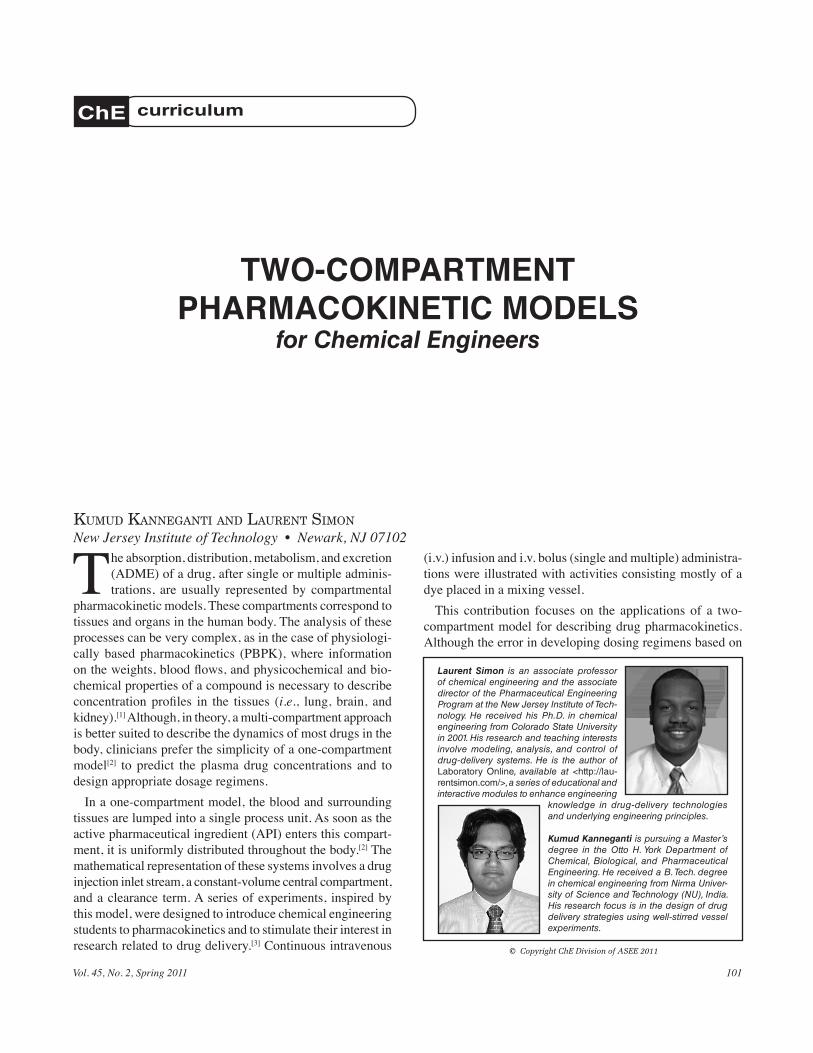
The schematic of a two-compartment model is shown in Figure 1a. According to this representation, the human body is comprised of a central compartment consisting of the blood/plasma and well-perfused tissues (e.g., liver, heart), and a peripheral compartment mainly composed of poorly perfused tissues (e.g., skeletal muscles). Analysis of a blood sample would reveal the concentration in the first compart-ment. This measurement may be used by the physician to assess the effectiveness of a drug-dosage regimen.
Component balances in the two compartments (Figure 1a) yield:
d C Vdt
k C V k C V k C Vel l1 1
1 12 1 1 21 2 2 1( )
=− − + ( )
and
d C Vdt
k C V k C V2 212 1 1 21 2 2 2
( )= − , ( )
where C is the drug concentration, V is the volume, and k is a mass transfer rate constant. The subscripts 1 and 2 repre-sent the central and peripheral compartments, respectively. Drug elimination is shown by the subscript el. In addition, the subscript 12 denotes a transfer from compartment 1 to compartment 2 while drug transfer in the opposite direction is shown by 21. The parameter kel is a first-order elimination rate constant, which is often used to represent clearance. It should be noted that more complex expressions (e.g., Mi-chaelis-Menten kinetics) are often appropriate for certain drugs. Since the volumes are constant, Eqs. (1) and (2) can be written as:[4]
d Cdt
k C k C k Cel l1
12 1 21 21 2 3( )=− − + ζ ( )
and
ζ ζ212
12 1 21 21 2 4d Cdt
k C k C( )
= − ( )
with ζ212
1
=VV.
Figure 1b. corresponds to the flowchart of a two-unit pro-cess designed to mimic the behavior of a two-compartment model. Several pumps are required to manipulate the flow rates. Fresh water streams are also added to the vessels. At this point, students may be asked to show that component balances around the units lead to the system described by Eqs. (3) and (4) (objectives i and ii). A total mass balance around vessels 1 and 2 yields:
d Vdt
F F F Fw w el l
ρρ ρ ρ ρ1 1
1 1 21 2 12 1 5( )
= + − − ( )
and d Vdt
F F Fw w
ρρ ρ ρ2 22 2 12 1 21 2 6
( )= + − , ( )
respectively. The subscripts w1 and w2 indicate the fresh wa-ter streams into vessels 1 and 2. Assuming equal and constant densities, we have ρ ρ ρ ρ1 2 1 2= = =w w . The relationships:
F F F Fel w+ = +12 1 21 7( )
and
F F Fw21 2 12 8= + ( )
Figure 1. Representation of a two-compartment model. Figure 1a is a schematic model of the process as intro-duced in a course in pharmacokinetics; Figure 1b is the
two-unit process that is assembled to mimic the behavior of the two-compartment model.
Vol. 45, No. 2, Spring 2011 103
hold in order to maintain constant volumes in both tanks. In addition, potassium permanganate balances around the two units yield:
d C Vdt
F C F C F Cel l1 1
21 2 12 1 9( )
= − − ( )
and
d C Vdt
F C F C2 212 1 21 2 10
( )= − . ( )
Dividing Eqs. (9) and (10) by V1 results in Eqs. (3) and (4)
with kFV
kFV
kFV
VVel
el12
12
121
21
2 121
2
1
= = = =, , , .ζ
The experiments are conducted with V1=V2. As a result, Eqs. (3) and (4) become:
d Cdt
k C k C k Cel l1
12 1 21 2 11( )=− − + ( )
and
d Cdt
k C k C212 1 21 2 12
( )= − ( )
The initial conditions are C1(0) = C10 and C2(0) = 0 for a bo-lus injection. Using the Laplace transforms of the concentra-
tions C1(t) and C2(t) (i.e., L C t C s C t e dtst1 1 1
0
( ){ }= ( )= ( )∞
−∫
and L C t C s C t e dtst2 2 2
0
( ){ }= ( )= ( )∞
−∫ ) and applying the
Laplace operator to both sides of Eqs. (11) and (12), the fol-lowing equations are obtained:
sC C k k C k Cel1 10 12 1 21 2 13− =− +( ) + ( )
and
sC k C k C2 12 1 21 2 14= − ( )
The system formed by Eqs. (13) and (14) is solved to give:
Cs k C
s k k k s k kel el1
21 10
212 21 21
15=+( )
+ + +( ) +( )( )
and
Ck C
s k k k s k kel el2
12 102
12 21 21
16=+ + +( ) +( )
( )
Partial-fraction expansion, or the residue theorem, may be used to invert the C andC1 2 (objective iii). Students are also encouraged to apply Laplace transform initial and final value theorems to verify the correctness of Eqs. (15) and (16).
Although the satisfaction of the initial conditions, C1(0) = C10 and C2(0) = 0, is not sufficient to guarantee the accuracy of Eqs. (15) and (16), these equalities are necessary conditions. In addition, showing that C t C t1 2 0→∞( )= →∞( )= may lead to a discussion on the necessity for administering multiple bolus i.v. doses.
C tk C
ek C
t1
21 10 21 10( )=+( )−( )
−+( )−
+
+ −
−
+
+λ
λ λ
λ
λλ
λλλ
−( )−
e t ( )17
and
C tk C
ek C
et t2
12 10 12 10 1( )=−( )
−−( )+ − + −
+ −
λ λ λ λλ λ ( 88)
with
λ+ =− + +( )+ + +( ) −k k k k k k k kel el el12 21 12 21
2
214
21( 99)
and
λ− =− + +( )− + +( ) −k k k k k k k kel el el12 21 12 21
2
214
22( 00)
Given concentration data in the central compartment (or vessel 1), Eq. (17) can be applied to estimate k12, k21, and k el (objective iv). Students may be given the opportunity to choose among three methods to compute these parameters:
1) Measurement of the flow rates: the pharmacokinetics are
calculated using kFV
kFV
and kFVel
el12
12
121
21
2 1
= = =, , .
2) Regression of Eq. (17) to experimental C1(t) data: Eq. (17) is written in the form C t Ae Be witht t
1( )= + >− −α β α β. Computational software packages such as Math-ematica® (Wolfram Research, Inc., IL) or Matlab® (The MathWorks, Inc., MA) can be adopted to estimate A, B, α, and β. Algebraic manipulations show that
k A BA B
kk
and k k kel el2121
12 21=++
= = + − −β α αβ
α β, .
3) Methods of residuals[5]: Data collected at long times are fitted to the equation C1l(t) = Be t−β because α > β. Pa-rameters B and β are obtained from ln[C1l(t)]=ln(B)– βt. The variable C1l represents the concentration at a suf-ficiently long time. Similarly, data gathered at short times are fitted to C1s(t)–Be
t−β =Ae t−α where C1s stands for the concentration a short time after the bolus injection. Parameters A and α are estimated from ln[Cls(t)–Be
t−β ] =ln(A)–αt.
Any of the methodologies described above is implemented to study the influences of pharmacokinetic parameters on C1 and C2.
Chemical Engineering Education104
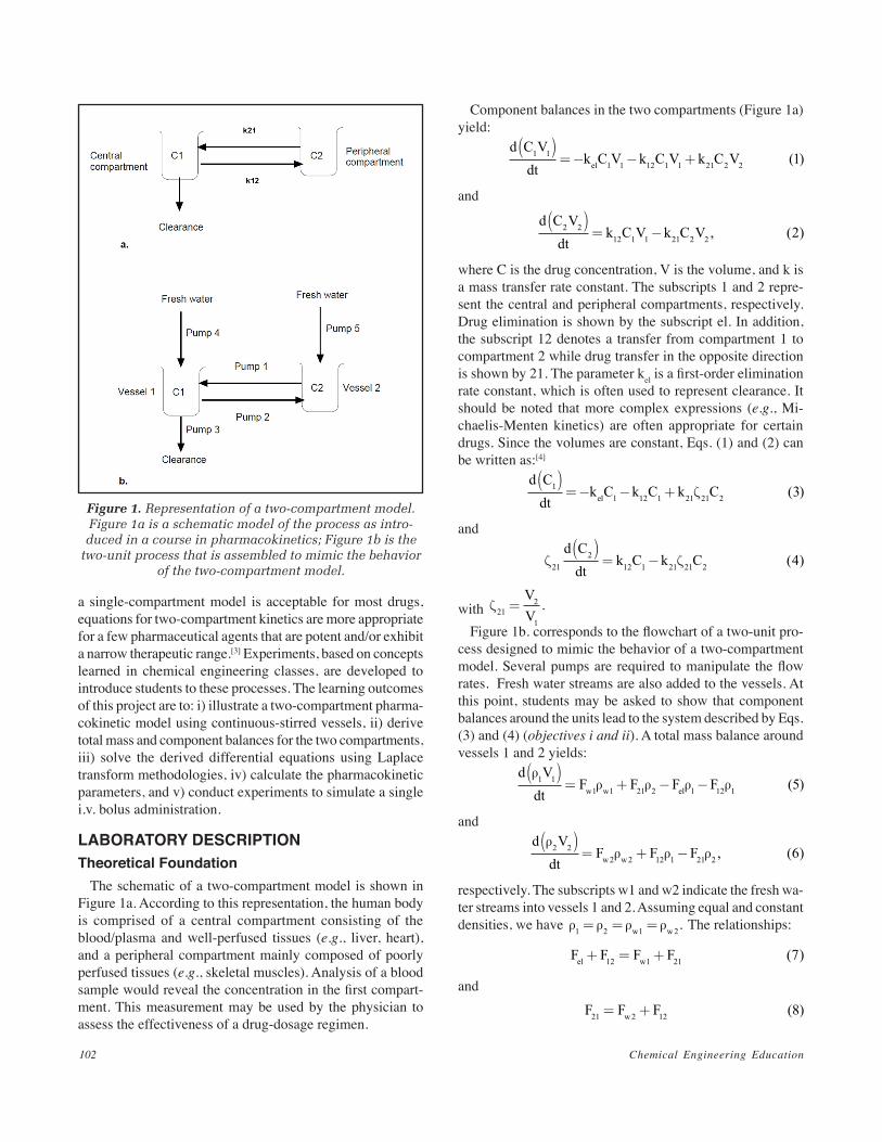
Materials and Experimental Procedure Except for the increased number of pumps, the same
materials required in the study of the one-compartment experiments[3] are used in this project (Figure 2) (objective v): variable flow-rate pumps, beakers, stopwatch, graduated cylinders, pipettes, rubber tubing, magnetic stirrer, magnetic bars, potassium permanganate, spectrophotometer, cuvettes, laboratory stands, and clamps. An i.v. bolus of 1.37 g of potas-sium permanganate was administered to the central compart-ment. Samples were collected every 15 minutes for both the central and the peripheral compartments and analyzed with a spectrophotometer set at 530 nm. A calibration curve was developed to relate the concentration with the absorbance reading: y = 0.0163A where y represented the concentration in g/mL and A the absorbance. The volume of each vessel was maintained at 200 mL.
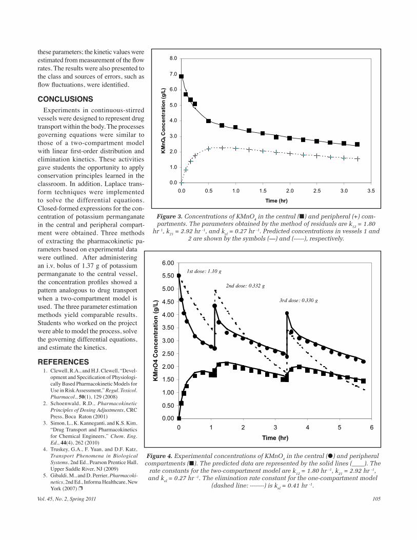
Results and Discussions The data for the i.v. bolus administration are shown in Fig-
ure 3. Pharmacokinetic parameters determined from the three methods are k12 = 1.80 hr-1, k21 = 2.94 hr-1, and kel = 0.30 hr-1 (measurement of the flow rates); k12 = 1.42 hr-1, k21 = 2.37 hr-1, and kel = 0.26 hr-1 (regression in Mathematica®); k12 = 1.80 hr-1, k21 = 2.92 hr-1, and kel = 0.27 hr-1(methods of residuals). The predicted concentrations plotted are the ones derived by the third method. Students may be given a project where they are expected to investigate the effects of the kinetic parameters on C1 and C2 to understand how drug transport is influenced by the distribution and elimination rate constants. This research also offers the opportunity to address the effects of the dose size on the plasma blood concentration. Multiple bolus-injec-tions and constant-rate infusions can also be studied after a slight modification of the model and initial conditions.
The choice of one compartment or two compartments may be an important factor when designing appropriate drug-dos-
ing regimens. To illustrate this point, three bolus injections of 1.10 g, 0.33 g, and 0.33 g of potassium permanganate were added to the central compartment at 0, 1.12, and 3.36 hours, respectively, as recommended by the results of an optimal dosing regimen for KMnO4 (Figure 4). The optimization code, based on a two-compartment model and written in the Mathematica® environment, minimized the sum of squared errors between the concentrations in the central compartment and a desired KMnO4 level of 3.46 g/L for an experimental duration of 5.75 hours. The following observations can be made: i) The predicted and experimental data agree very well and ii) the calculated doses were able to maintain the KMnO4 concentration around 3.46 g/L. Simulations conducted under the assumption that KMnO4 obeys one-compartment pharma-cokinetics show that the predicted data deviate considerably from the true profile (Figure 4).
SUMMARY OF EXPERIENCES A group of six students from an undergraduate course in
biotransport worked on this project. The three-credit class is designed for biomedical engineering students pursuing tracks in biomaterials and tissue engineering or biomechanics.[3] Chemical engineering students may also select the course as an elective toward their degree requirements. A final report was produced after several meetings with the instructor dur-ing which the project was discussed. Although a graduate assistant helped design the experimental setup (Figure 2) because of time limitation, the group was required to draw a schematic diagram of the process similar to Figure 1b. The specific assignment was to study the effects of loading doses on the concentrations in the central and peripheral compart-ments. In addition to providing a background of the subject, the students were also responsible for deriving the model equations and estimating the kinetic parameters. They were not told about the methods that could be applied to determine
Figure 2. The experi-mental setup of the two-
compartment model. Potassium permanga-nate was added to the
beakers. Fresh water in an Erlenmeyer flask was introduced to the
two compartments.
Vol. 45, No. 2, Spring 2011 105
these parameters; the kinetic values were estimated from measurement of the flow rates. The results were also presented to the class and sources of errors, such as flow fluctuations, were identified.
CONCLUSIONS Experiments in continuous-stirred
vessels were designed to represent drug transport within the body. The processes governing equations were similar to those of a two-compartment model with linear first-order distribution and elimination kinetics. These activities gave students the opportunity to apply conservation principles learned in the classroom. In addition, Laplace trans-form techniques were implemented to solve the differential equations. Closed-formed expressions for the con-centration of potassium permanganate in the central and peripheral compart-ment were obtained. Three methods of extracting the pharmacokinetic pa-rameters based on experimental data were outlined. After administering an i.v. bolus of 1.37 g of potassium permanganate to the central vessel, the concentration profiles showed a pattern analogous to drug transport when a two-compartment model is used. The three parameter estimation methods yield comparable results. Students who worked on the project were able to model the process, solve the governing differential equations, and estimate the kinetics.
REFERENCES 1. Clewell, R.A., and H.J. Clewell, “Devel-
opment and Specification of Physiologi-cally Based Pharmacokinetic Models for Use in Risk Assessment,” Regul. Toxicol. Pharmacol., 50(1), 129 (2008)
2. Schoenwald, R.D., Pharmacokinetic Principles of Dosing Adjustments, CRC Press, Boca Raton (2001)
3. Simon, L., K. Kanneganti, and K.S. Kim, “Drug Transport and Pharmacokinetics for Chemical Engineers,” Chem. Eng. Ed., 44(4), 262 (2010)
4. Truskey, G.A., F. Yuan, and D.F. Katz, Transport Phenomena in Biological Systems, 2nd Ed., Pearson Prentice Hall, Upper Saddle River, NJ (2009)
5. Gibaldi, M., and D. Perrier, Pharmacoki-netics, 2nd Ed., Informa Healthcare, New York (2007) p
0.0
1.0
2.0
3.0
4.0
5.0
6.0
7.0
8.0
0.0 0.5 1.0 1.5 2.0 2.5 3.0 3.5
Time (hr)
KM
nO4 C
once
ntra
tion
(g/L
)
0.00
0.50
1.00
1.50
2.00
2.50
3.00
3.50
4.00
4.50
5.00
5.50
6.00
0 1 2 3 4 5 6
Time (hr)
KM
nO4
Con
cent
ratio
n (g
/L)
1st dose: 1.10 g
2nd dose: 0.332 g
3rd dose: 0.330 g
Figure 3. Concentrations of KMnO4 in the central (j) and peripheral (+) com-partments. The parameters obtained by the method of residuals are k12 = 1.80
hr- 1, k21 = 2.92 hr -1, and kel = 0.27 hr -1. Predicted concentrations in vessels 1 and 2 are shown by the symbols (—) and (-----), respectively.
Figure 4. Experimental concentrations of KMnO4 in the central (d) and peripheral compartments (j). The predicted data are represented by the solid lines (____). The
rate constants for the two-compartment model are k12 = 1.80 hr -1, k21 = 2.92 hr -1, and kel = 0.27 hr -1. The elimination rate constant for the one-compartment model
(dashed line: -------) is kel = 0.41 hr -1.
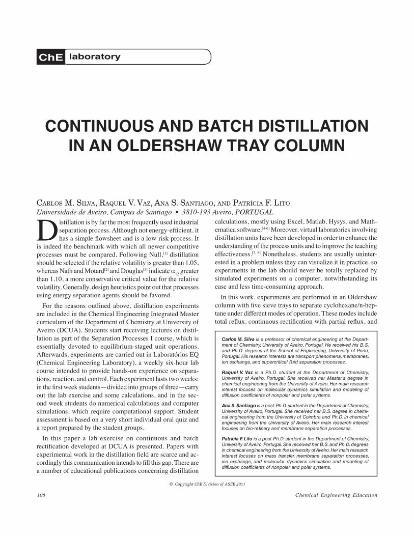
Chemical Engineering Education106
Distillation is by far the most frequently used industrial separation process. Although not energy-efficient, it has a simple flowsheet and is a low-risk process. It
is indeed the benchmark with which all newer competitive processes must be compared. Following Null,[1] distillation should be selected if the relative volatility is greater than 1.05, whereas Nath and Motard[2] and Douglas[3] indicate α12 greater than 1.10, a more conservative critical value for the relative volatility. Generally, design heuristics point out that processes using energy separation agents should be favored.
For the reasons outlined above, distillation experiments are included in the Chemical Engineering Integrated Master curriculum of the Department of Chemistry at University of Aveiro (DCUA). Students start receiving lectures on distil-lation as part of the Separation Processes I course, which is essentially devoted to equilibrium-staged unit operations. Afterwards, experiments are carried out in Laboratórios EQ (Chemical Engineering Laboratory), a weekly six-hour lab course intended to provide hands-on experience on separa-tions, reaction, and control. Each experiment lasts two weeks: in the first week students—divided into groups of three—carry out the lab exercise and some calculations, and in the sec-ond week students do numerical calculations and computer simulations, which require computational support. Student assessment is based on a very short individual oral quiz and a report prepared by the student groups.
In this paper a lab exercise on continuous and batch rectification developed at DCUA is presented. Papers with experimental work in the distillation field are scarce and ac-cordingly this communication intends to fill this gap. There are a number of educational publications concerning distillation
calculations, mostly using Excel, Matlab, Hysys, and Math-ematica software.[4-6] Moreover, virtual laboratories involving distillation units have been developed in order to enhance the understanding of the process units and to improve the teaching effectiveness.[7, 8] Nonetheless, students are usually uninter-ested in a problem unless they can visualize it in practice, so experiments in the lab should never be totally replaced by simulated experiments on a computer, notwithstanding its ease and less time-consuming approach.
In this work, experiments are performed in an Oldershaw column with five sieve trays to separate cyclohexane/n-hep-tane under different modes of operation. These modes include total reflux, continuous rectification with partial reflux, and
CONTINUOUS AND BATCH DISTILLATION IN AN OLDERSHAW TRAY COLUMN
CarloS m. Silva, raquEl v. vaz, ana S. Santiago, and patríCia F. lito
Universidade de Aveiro, Campus de Santiago • 3810-193 Aveiro, PORTUGAL
© Copyright ChE Division of ASEE 2011
ChE laboratory
Carlos M. Silva is a professor of chemical engineering at the Depart-ment of Chemistry, University of Aveiro, Portugal. He received his B.S. and Ph.D. degrees at the School of Engineering, University of Porto, Portugal. His research interests are transport phenomena, membranes, ion exchange, and supercritical fluid separation processes.
Raquel V. Vaz is a Ph.D. student at the Department of Chemistry, University of Aveiro, Portugal. She received her Master’s degree in chemical engineering from the University of Aveiro. Her main research interest focuses on molecular dynamics simulation and modeling of diffusion coefficients of nonpolar and polar systems.
Ana S. Santiago is a post-Ph.D. student in the Department of Chemistry, University of Aveiro, Portugal. She received her B.S. degree in chemi-cal engineering from the University of Coimbra and Ph.D. in chemical engineering from the University of Aveiro. Her main research interest focuses on bio-refinery and membrane separation processes.
Patrícia F. Lito is a post-Ph.D. student in the Department of Chemistry, University of Aveiro, Portugal. She received her B.S. and Ph.D. degrees in chemical engineering from the University of Aveiro. Her main research interest focuses on mass transfer, membrane separation processes, ion exchange, and molecular dynamics simulation and modeling of diffusion coefficients of nonpolar and polar systems.
Vol. 45, No. 2, Spring 2011 107
batch rectification with constant reflux. An Oldershaw tray column is a laboratory-scale column equipped with perforated trays. Of special importance is the fact that it exhibits a sepa-ration capacity close to that of large industrial columns.[9] In fact, experimental results show that commercial towers will require a similar number of stages to reach the same separa-tion level obtained in the Oldershaw unit.[10]
With this work students practice relevant concepts in-troduced earlier in their curriculum, namely vapor-liquid equilibrium, continuous vs. batch operation, McCabe-Thiele graphical method, column efficiency, and application of the generalized Rayleigh equation. Moreover, students use in-dustrial simulation software (Aspen) to predict experimental results, giving them the opportunity to improve their skills in this field, too. By examining experimental results and compar-ing them with those obtained from simulations, students gain insight to this unit operation.
LABORATORY DESCRIPTION Experimental Setup
Experiments are performed in an Oldershaw tray column instrumented and equipped with a control system supplied by Normschliff Gerätebau (similar equipment is available from Normag GmbH Imenau). Other commercial teaching equipment for continuous distillation is offered, for example, by Armfield, Ltd. (<www.discoverarmfield.co.uk>), De Dietrich-QVF (<www.ddpsinc.com>), and Phywe (<www.phywe-systeme.com>). The unit used is shown in Figure 1 and comprises five perforated plates (3 cm of diameter), a reboiler
(capacity of 2 L), a total top condenser us-ing tap water as cooling fluid, a lateral con-denser to re-move distillate as liquid, and a solenoid valve to divide the vapor stream into reflux and distillate un-der the partial reflux mode. Additional fea-tures include: s a m p l i n g points above each tray to de-termine liquid composition; and tempera-
ture sensors immersed in the reboiler and located in the top condenser allowing the determination of the bottom and head compositions, respectively. The column is used to separate c.a. 800 mL of a cyclohexane (Lab-Scan, 99%) / n-heptane (Lab-Scan, 99%) mixture with 30% (mol) of cyclohexane.
The calibration curve—measured in this work—to deter-mine the cyclohexane mole fraction (x1) in a cyclohexane–n-heptane mixture at 30 ̊ C as function of refractive index (RI), is given by x1=-309.95 RI2 + 895.15 RI – 645.15.
Experiments at Total Reflux, R = ∞ Rectifications at total reflux were performed at two distinct
effective reboiler powers (P = 75 and 125 W) to evaluate the effect of the internal molar flow upon separation and column efficiency. The invariance of the top and bottom (TD and TB) temperatures was used to detect the steady state. Ad-ditionally, they were utilized to determine the corresponding cyclohexane molar compositions, xD and xB, by vapor-liquid equilibrium calculations assuming that the column is kept at atmospheric pressure (pressure drop along the column is considered negligible).
Continuous Rectification at Partial Reflux This Oldershaw tray column is extremely versatile. It can
be operated continuously under partial reflux. With simple modifications, the distillate may be directly fed to the reboiler (see path A in Figure 1), allowing us to reach the correspond-ing steady state. Such an experiment was carried out at R = 6 for P = 125 W. Once more, TD and TB were utilized to determine xD and xB.
Batch Rectification at Constant Partial Reflux Finally, a semi-continuous or batch distillation was performed
for R = 6 and P = 125 W. Presently, the distillate is not fed to the reboiler, but collected in the independent flask shown in Figure 1 (see path B). Under such mode of operation, compo-sitions vary along time. TD and TB were registered during 1 h approximately, to calculate the corresponding xD and xB, and the distillate refractive index was measured at the end.
HAZARDS AND SAFETY PRECAUTIONS Cyclohexane (CAS registry number: 110-82-7) and
n-heptane (CAS registry number: 142-82-5) are stable liquids at room temperature, highly flammable, and may readily form explosive mixtures with air. They are harm-ful if swallowed or inhaled, and cause irritation to skin, eyes, and respiratory tract. Attention must be paid during the withdrawal of liquid samples, from the bottom of the column, in order to measure the refractive index. Protec-tion equipment, including gloves and glasses, should be used. Students must review the Materials Safety Data Sheet for each chemical before starting the experiment and are instructed to collect wastes in specific tanks to be subsequently treated by the DCUA.
Figure 1. Oldershaw tray column.
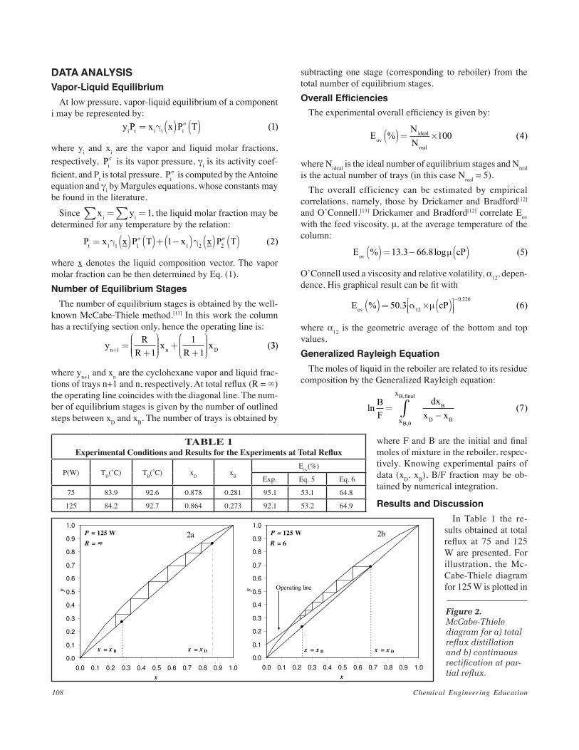
Chemical Engineering Education108
DATA ANALYSIS Vapor-Liquid Equilibrium
At low pressure, vapor-liquid equilibrium of a component i may be represented by:
y P x x P Ti t i i i= ( ) ( )γ σ ( )1
where yi and xi are the vapor and liquid molar fractions, respectively, Pi
σ is its vapor pressure, γi is its activity coef-ficient, and Pt is total pressure. Pi
σ is computed by the Antoine equation and γi by Margules equations, whose constants may be found in the literature.
Since x yi i∑ ∑= =1, the liquid molar fraction may be determined for any temperature by the relation:
P x x P T x x P Tt = ( ) ( )+ −( ) ( ) ( )1 1 1 1 2 21 2γ γσ σ ( )
where x denotes the liquid composition vector. The vapor molar fraction can be then determined by Eq. (1). Number of Equilibrium Stages
The number of equilibrium stages is obtained by the well-known McCabe-Thiele method.[11] In this work the column has a rectifying section only, hence the operating line is:
y RR
xR
xn n D+ = +
+
+
1 1
11
(33)
where yn+1 and xn are the cyclohexane vapor and liquid frac-tions of trays n+1 and n, respectively. At total reflux (R = ∞) the operating line coincides with the diagonal line. The num-ber of equilibrium stages is given by the number of outlined steps between xD and xB. The number of trays is obtained by
subtracting one stage (corresponding to reboiler) from the total number of equilibrium stages.Overall Efficiencies
The experimental overall efficiency is given by:
ENNov
ideal
real
% ( )( )= ×100 4
where Nideal is the ideal number of equilibrium stages and Nreal is the actual number of trays (in this case Nreal = 5).
The overall efficiency can be estimated by empirical correlations, namely, those by Drickamer and Bradford[12] and O’Connell.[13] Drickamer and Bradford[12] correlate Eov with the feed viscosity, μ, at the average temperature of the column:
E cPov % . . log ( )( )= − ( )13 3 66 8 5µ
O’Connell used a viscosity and relative volatility, α12, depen-dence. His graphical result can be fit with
E cPov % . ( ).
( )= × ( )
−
50 3 612
0 226α µ
where α12 is the geometric average of the bottom and top values. Generalized Rayleigh Equation
The moles of liquid in the reboiler are related to its residue composition by the Generalized Rayleigh equation:
ln ( ),
,BF
dxx xx
x
B
B finalB
D B
=−∫
0
7
where F and B are the initial and final moles of mixture in the reboiler, respec-tively. Knowing experimental pairs of data (xD, xB), B/F fraction may be ob-tained by numerical integration.
Results and Discussion In Table 1 the re-
sults obtained at total reflux at 75 and 125 W are presented. For illustration, the Mc-Cabe-Thiele diagram for 125 W is plotted in
0.0
0.1
0.2
0.3
0.4
0.5
0.6
0.7
0.8
0.9
1.0
0.0 0.1 0.2 0.3 0.4 0.5 0.6 0.7 0.8 0.9 1.0
x
y
P = 125 W
R = ∞2a
x = x B x = x D
0.0
0.1
0.2
0.3
0.4
0.5
0.6
0.7
0.8
0.9
1.0
0.0 0.1 0.2 0.3 0.4 0.5 0.6 0.7 0.8 0.9 1.0
x
y Operating line
x = x B x = x D
P = 125 W
R = 6
2b
Figure 2. McCabe-Thiele diagram for a) total reflux distillation and b) continuous rectification at par-tial reflux.
TABLE 1Experimental Conditions and Results for the Experiments at Total Reflux
P(W) TD(˚C) TB(˚C) xD xB
Eov(%)
Exp. Eq. 5 Eq. 6
75 83.9 92.6 0.878 0.281 95.1 53.1 64.8
125 84.2 92.7 0.864 0.273 92.1 53.2 64.9
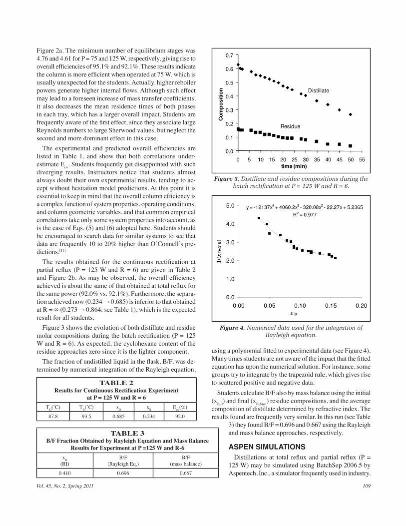
Vol. 45, No. 2, Spring 2011 109
Figure 2a. The minimum number of equilibrium stages was 4.76 and 4.61 for P = 75 and 125 W, respectively, giving rise to overall efficiencies of 95.1% and 92.1%. These results indicate the column is more efficient when operated at 75 W, which is usually unexpected for the students. Actually, higher reboiler powers generate higher internal flows. Although such effect may lead to a foreseen increase of mass transfer coefficients, it also decreases the mean residence times of both phases in each tray, which has a larger overall impact. Students are frequently aware of the first effect, since they associate large Reynolds numbers to large Sherwood values, but neglect the second and more dominant effect in this case.
The experimental and predicted overall efficiencies are listed in Table 1, and show that both correlations under- estimate Eov. Students frequently get disappointed with such diverging results. Instructors notice that students almost always doubt their own experimental results, tending to ac-cept without hesitation model predictions. At this point it is essential to keep in mind that the overall column efficiency is a complex function of system properties, operating conditions, and column geometric variables, and that common empirical correlations take only some system properties into account, as is the case of Eqs. (5) and (6) adopted here. Students should be encouraged to search data for similar systems to see that data are frequently 10 to 20% higher than O’Connell’s pre-dictions.[11]
The results obtained for the continuous rectification at partial reflux (P = 125 W and R = 6) are given in Table 2 and Figure 2b. As may be observed, the overall efficiency achieved is about the same of that obtained at total reflux for the same power (92.0% vs. 92.1%). Furthermore, the separa-tion achieved now (0.234→ 0.685) is inferior to that obtained at R = ∞ (0.273→ 0.864; see Table 1), which is the expected result for all students.
Figure 3 shows the evolution of both distillate and residue molar compositions during the batch rectification (P = 125 W and R = 6). As expected, the cyclohexane content of the residue approaches zero since it is the lighter component.
The fraction of undistilled liquid in the flask, B/F, was de-termined by numerical integration of the Rayleigh equation,
using a polynomial fitted to experimental data (see Figure 4). Many times students are not aware of the impact that the fitted equation has upon the numerical solution. For instance, some groups try to integrate by the trapezoid rule, which gives rise to scattered positive and negative data.
Students calculate B/F also by mass balance using the initial (xB,0) and final (xB,final) residue compositions, and the average composition of distillate determined by refractive index. The results found are frequently very similar. In this run (see Table
3) they found B/F = 0.696 and 0.667 using the Rayleigh and mass balance approaches, respectively.
ASPEN SIMULATIONS Distillations at total reflux and partial reflux (P =
125 W) may be simulated using BatchSep 2006.5 by Aspentech, Inc., a simulator frequently used in industry.
TABLE 2Results for Continuous Rectification Experiment
at P = 125 W and R = 6TD(˚C) TB(˚C) xD xB Eov(%)
87.8 93.5 0.685 0.234 92.0
TABLE 3B/F Fraction Obtained by Rayleigh Equation and Mass Balance
Results for Experiment at P =125 W and R-6xD
(RI) B/F
(Rayleigh Eq.) B/F
(mass balance)
0.410 0.696 0.667
y = -12137x4 + 4060.2x3 - 320.08x2 - 22.27x + 5.2365
R2 = 0.977
0.0
1.0
2.0
3.0
4.0
5.0
0.00 0.05 0.10 0.15 0.20
x B
1/(
xD-x
B)
0.0
0.1
0.2
0.3
0.4
0.5
0.6
0.7
0 5 10 15 20 25 30 35 40 45 50 55
Co
mp
osit
ion
time (min)
Distillate
Residue
Figure 3. Distillate and residue compositions during the batch rectification at P = 125 W and R = 6.
Figure 4. Numerical data used for the integration of Rayleigh equation.

Chemical Engineering Education110
This software allows the simulation of distillation columns under different operating conditions and modes of operation. The embedded VLE calculations were based on the RK-SOAVE method. Total Reflux Simulation
The total reflux simulation is carried out using the input specifications and additional information shown in Table 4. For this case, the column is as-sumed to be initially filled with nitrogen, therefore a partial condenser has to be selected in order to purge it from the system. A feed stream was imposed dur-
ing a predetermined time to charge the tower with the same number of moles that our Oldershaw column contains initially. Subsequently, a null distillate flow must be imposed to reach total reflux condition (see Figure 5). The simulation is carried out in two consecutive steps: i) column charge and ii) distillation at total reflux. Table 5 compiles the pertinent data and options selection for the total reflux calcula-tions, in order to help students to reproduce our results.
Simulation of Continuous Rectification at Partial Reflux The continuous rectification at partial reflux (R = 6) is computed
with the input specifications and additional information compiled in Table 6 ( page 112). For this simulation, the column has to be initially at total reflux and only then submitted to R = 6. Students should realize this approach is in accordance with industrial columns start-up: distillation towers are frequently started up at total reflux, after an initial charge of feed, and this condition runs until both distillate and bottom compositions reach the desired project specifications; only then is the finite reflux ratio implemented.[14] In our case, R = 6, the column holdups and pressure drop values are those obtained previously from the total reflux simulation, and the feed stream is the distillate recycled to column (see Figure 6, page 112). Table 7 (page 113) compiles data and options for the continuous rectification at partial reflux calculations.
Simulation Results The simulation results, presented in Table 8 (page 113) for both total
and partial reflux, are in good agreement with the measured values; the relative deviations found lie between 1.0 and 19.3%, being higher for R = 6. The calculated separation for R = ∞ (xD – xB = 0.584) is very near the experimental one (xD – xB = 0.591) whereas it diverges for R = 6 (0.484 against 0.451, respectively). It is curious to notice that students usually doubt their experimental observations against the simulated results, sug-gesting possible experimental errors for the deviations found for R = 6. Nonetheless, in this case such large error may be attributed to the fact that some operating parameters, including pressure drop and holdups, were calculated at R = ∞ and assumed to be the same in the continuous partial reflux simulation. On the whole, students and instructors are amazed with simulation results due to the large number of input parameters and specifications, particularly those for geometrical variables.
CONCLUSIONS This work describes
an experiment in which students have the op-portunity to study dis-tillation, using an Old-ershaw tray column, under three different modes of operation: total reflux, continuous partial reflux, and batch with constant reflux. The effect of the internal molar flows on column
TABLE 4Information for Aspen Simulation
at Total RefluxInput Specifications
- Column initially empty (initially filled with N2)
- Partial condenser
- Feed stream to introduce the initial charge of mixture
- Null distillate flow to get ∞ = R
Additional Information
- Column configuration (number of stages, including reboiler and condenser)
- Reboiler geometry (dimensions and jacket type)
- Power (P = 125 W)
- Condenser specifications (pressure, type, area, con-densing coefficient, coolant inlet temperature, coolant mass flow, and coolant heat capacity)
- Tray specifications and dimensions
Operation Steps
- i) Column charge
- ii) Distillation at ∞=R
Results
- Column holdups
- Pressure drop
- Composition profile
- Temperature profile
Figure 5. Detail of an Aspen BatchSep 2006.5 window for the total reflux simulation.
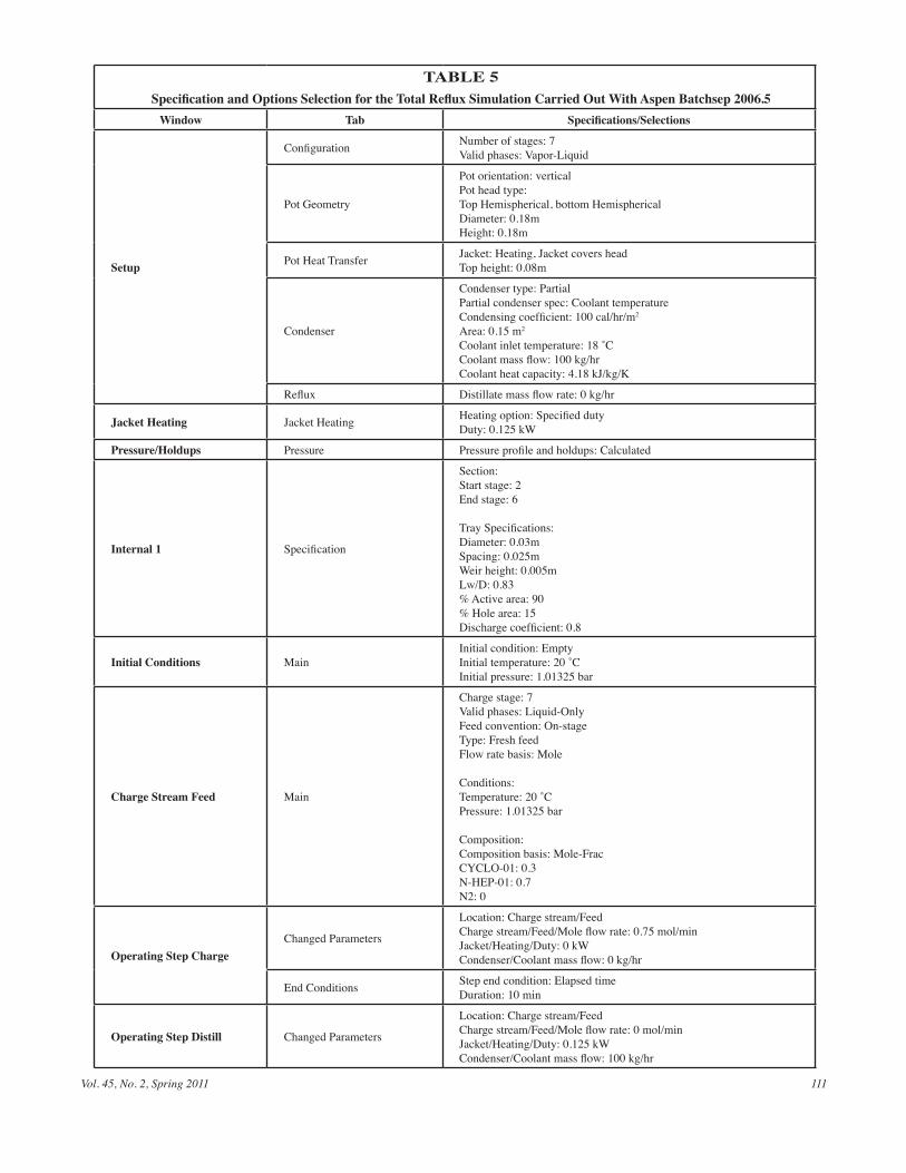
Vol. 45, No. 2, Spring 2011 111
TABLE 5Specification and Options Selection for the Total Reflux Simulation Carried Out With Aspen Batchsep 2006.5
Window Tab Specifications/Selections
Setup
Configuration Number of stages: 7Valid phases: Vapor-Liquid
Pot Geometry
Pot orientation: vertical Pot head type: Top Hemispherical, bottom Hemispherical Diameter: 0.18m Height: 0.18m
Pot Heat Transfer Jacket: Heating, Jacket covers head Top height: 0.08m
Condenser
Condenser type: Partial Partial condenser spec: Coolant temperature Condensing coefficient: 100 cal/hr/m2 Area: 0.15 m2 Coolant inlet temperature: 18 ˚C Coolant mass flow: 100 kg/hr Coolant heat capacity: 4.18 kJ/kg/K
Reflux Distillate mass flow rate: 0 kg/hr
Jacket Heating Jacket Heating Heating option: Specified duty Duty: 0.125 kW
Pressure/Holdups Pressure Pressure profile and holdups: Calculated
Internal 1 Specification
Section: Start stage: 2 End stage: 6
Tray Specifications: Diameter: 0.03m Spacing: 0.025m Weir height: 0.005m Lw/D: 0.83 % Active area: 90 % Hole area: 15 Discharge coefficient: 0.8
Initial Conditions Main Initial condition: Empty Initial temperature: 20 ˚C Initial pressure: 1.01325 bar
Charge Stream Feed Main
Charge stage: 7 Valid phases: Liquid-Only Feed convention: On-stage Type: Fresh feed Flow rate basis: Mole
Conditions: Temperature: 20 ˚C Pressure: 1.01325 bar
Composition: Composition basis: Mole-Frac CYCLO-01: 0.3 N-HEP-01: 0.7 N2: 0
Operating Step Charge Changed Parameters
Location: Charge stream/FeedCharge stream/Feed/Mole flow rate: 0.75 mol/min Jacket/Heating/Duty: 0 kW Condenser/Coolant mass flow: 0 kg/hr
End Conditions Step end condition: Elapsed time Duration: 10 min
Operating Step Distill Changed Parameters
Location: Charge stream/Feed Charge stream/Feed/Mole flow rate: 0 mol/min Jacket/Heating/Duty: 0.125 kW Condenser/Coolant mass flow: 100 kg/hr
Chemical Engineering Education112
performance was investigated at total reflux by changing reboiler power.
Results show that the efficiency decreases slightly with increasing flows. Moreover, column efficiency measured at partial reflux is analogous to that obtained at total reflux. For batch distillation, the application of the generalized Rayleigh equation provides good results. The results at infinite reflux and for the continuous rectification at partial reflux were com-pared with those obtained by Aspen BatchSep simulations, giving rise to relative deviations between 1.0 and 19.3%.
With this work students practice relevant concepts, includ-ing vapor-liquid equilibrium, continuous vs. batch operation, McCabe-Thiele graphical method, and column efficiency as
well as data analysis with the generalized Rayleigh equation. Furthermore, they are introduced to the use of simulation software, an important tool for their chemical engineering instruction.
ACKNOWLEDGMENTS Patrícia F. Lito and Ana Santiago wish to express their
gratitude to Fundação para a Ciência e Tecnologia (Portugal) for the grants provided (SFRH/BD/25580/2005 and SFRH/BPD/48258/2008), and to B.R. Figueiredo and Professor F. A. Da Silva for Aspen simulations and pictures support.
NOMENCLATURE B Final number of moles of liquid in the reboiler, mol Eov Overall efficiency, % F Initial number of moles of liquid in the reboiler, mol Nreal Number of real trays Nideal Ideal number of equilibrium stages P Reboiler power, W Pt Total pressure, atm Pσ Vapor pressure, atm R Reflux ratio RI Refractive index T Temperature, ˚C x Molar fraction of liquid phase y Molar fraction of vapor phase Greek letters α12 Relative volatility γ Activity coefficient μ Molar average liquid viscosity, cP Subscripts B Bottom D Top final Final condition i Component i 0 Initial condition
Figure 6. Continuous partial reflux simulation flowsheet.
TABLE 6Information for Aspen Simulation of the Continuous Rectification
at Partial RefluxInput Specifications
- Column initially at total reflux
- Total condenser
- Total initial charge and composition
- Distillate flow to get R = 6
Additional Information
- Column configuration (number of stages, including reboiler and condenser )
- Reboiler geometry (dimensions and jacket type)
- Power (P = 125 W)
- Column pressure drop and tray holdups
- Distillate charge stream (charge stage, type, temperature, pressure)
Operating Steps
- Distillation at R = 6
Results
- Composition profile
- Temperature profile

Vol. 45, No. 2, Spring 2011 113
TABLE 7Specification and Options Selection for the Continuous Rectification
at Partial Reflux Simulation Carried Out With Aspen Batchsep 2006.5Window Tab Specifications/Selections
Setup
Configuration Number of stages: 7 Valid phases: Vapor-Liquid
Pot Geometry
Pot orientation: vertical
Pot head type: Top Hemispherical, bottom Hemispherical Diameter: 0.18m Height: 0.18m
Pot Heat Transfer Jacket: Heating, Jacket covers head Top height: 0.08m
Condenser Condenser type: Total
Reflux Reflux ratio: 6
Jacket Heating Jacket Heating Heating option: Specified duty Duty: 0.125 kW
Pressure/Holdups Holdups Holdup basis: Mole Start Stage: 2 Stage Holdup: 5E-5 kmol
Initial Conditions
Main
Initial condition: Total reflux Initial drum liquid volume fraction: 0.5 Initial temperature: 20 ˚C Initial pressure: 1.01325 bar
Initial Charge
Composition basis: Mole-frac Total initial charge: 0.0075 kmol CYCLO-01: 0.3 N-HEP-01: 0.7
Charge Stream Distillate Main
Charge stage: 7 Valid phases: Liquid-Only Feed convention: On-stage Type: Distillate receiver recycle Flow rate basis: Mole
Conditions: Temperature: 80 ˚C Pressure: 1.01325 bar
Distillate receiver: 1
Operating Step Rpartial Changed Parameters
Location: Charge stream/Distillate Charge stream/Distillate/Mole flow rate: 0.1 mol/s Liquid distillate receiver: 1 Condenser pressure: 1.01325 Jacket/Heating/Duty: 0.125 kW
TABLE 8Total Reflux and Continuous Rectification Simulations ResultsBracketed values are relative deviations to the experimental ones.
TD(˚C) TB(˚C) xD xB
Total reflux (R = ∞) 83.8 92.1 0.873 (1.0%) 0.289 (5.9%)
Cont. rectification (R = 6) 85.6 92.4 0.774 (13.0%) 0.290 (19.3%)
REFERENCES 1. Null, H.R., “Selection of a
Separation Process,” in Hand-book of Separation Process Technology, Rousseau, R.W., Ed., Wiley-Interscience, New York (1987)
2. Nath, R., and R.L. Motard, “Evolutionary Synthesis of Separation Processes,” AIChE J., 27, 578-587 (1981)
3. Douglas, J.M., Conceptual Design of Chemical Process-es, McGraw-Hill, New York (1988)
4. van der Lee, J.H., D.G. Olsen, B.R. Young, and W.Y. Svrcek, “An Integrated, Real-Time Computing Environment for Advanced Process Control Development,” Chem. Eng. Ed., 35(3) 172 (2001)
5. Binous, H., “Equilibrium Staged Separations Using Mat-lab and Mathematica,” Chem. Eng. Ed., 42(2) 69 (2008)
6. Nasri, Z., and H. Binous, “Ap-plications of the Peng-Robin-son Equation of State Using Matlab,” Chem. Eng. Ed., 43(2) 115 (2009)
7. Santoro, M., and M. Mazzotti, “HYPER-TVT: Development and Implementation of an Inter-active Learning Environment for Students of Chemical and Process Engineering,” Chem. Eng. Ed., 43(2) 175 (2009)
8. Fleming, P.J., and M.E. Paulai-tis, “A Virtual Unit Operations Laboratory,” Chem. Eng. Ed., 36(2) 166 (2002)
9. Fair, J.R., H.R. Null, and W.L. Bolles, “Scale-up of Plate Efficiency From Laboratory Oldershaw Data,” Ind. Eng. Chem. Process Des. Dev., 22, 53-58 (1983)
10. Humphrey, J.L., and G.E. Keller, Separation Process Technology, McGraw-Hill, New York (1997)
11. Seader, J.D., and E.J. Henley, Separation Process Principles, 2nd Ed., John Wiley & Sons, New York (2006)
12. Drickamer, H.G., and J.R. Bradford, Transactions AIChE, 39, 319-360 (1943)
13. O’Connell, H.E., Transactions AIChE, 42, 741-755 (1946)
14. Foust, A.S., L.A. Wenzel, C.W. Clump, L. Maus, and L.B. Andersen, Principles of Unit Operations, 2nd Ed., John Wiley & Sons, New York (1980) p

Chemical Engineering Education114
Active learning is an umbrella term for instructional methods used in the classroom in which students are actively engaged in the learning process, as opposed
to a traditional lecture in which students play a passive role. Active learning can take many forms such as collaborative learning, cooperative learning, and problem-based learn-ing.[1] Research has shown that such nontraditional methods may lead to improved academic achievement, retention, and student attitudes toward learning, depending on the method of active learning utilized.[1,2] Indeed, Felder, et al.,[3] have in-cluded active learning methods on their list of teaching meth-ods that work. Courses on fluid mechanics are a particularly good match for active-learning techniques (see, for example, Reference 4), since everyday examples are ubiquitous.
In this paper, two active-learning modules targeted for use in an undergraduate fluid mechanics course are described. Materials for both have been designed and made avail-able via the Internet (<http://hrenya.colorado.edu/Hrenya.php?page=teaching>) so that they can be incorporated by interested educators with little time investment. These mod-ules involve several of the aforementioned forms of active learning, including both collaborative learning and coopera-tive learning.
The first activity involves a contest among small groups of students to correctly predict the outcome of tube-flow ex-periments using the mechanical energy balance. The students are first introduced to the experimental apparatus (gravity-driven flow from a tank), and then charged with predicting the outlet flow rates from various tubes. An announcement that prizes will be awarded to groups with predictions that best match the experimental data is also made at the start. The class culminates in the running of the experiments, and real-time identification of the “winners.” This class period allows the students to put their knowledge into practice via active-learning, while also providing a high level of energy
© Copyright ChE Division of ASEE 2011
ACTIVE LEARNING IN FLUID MECHANICS:YOUTUBE TUBE FLOW AND
PUZZLING FLUIDS QUESTIONS
ChriStinE m. hrEnya
University of Colorado • Boulder, CO 80309-0424
ChE classroom
Christine M. Hrenya received her degrees in chemical engineering from The Ohio State University (B.S.) and Carnegie Mellon Uni-versity (Ph.D.), and is currently on faculty at the Department of Chemical and Biological Engineering at the University of Colorado. Her research interests include granular and gas-solid flows, with an emphasis on polydis-persity, cohesion, and instabilities.
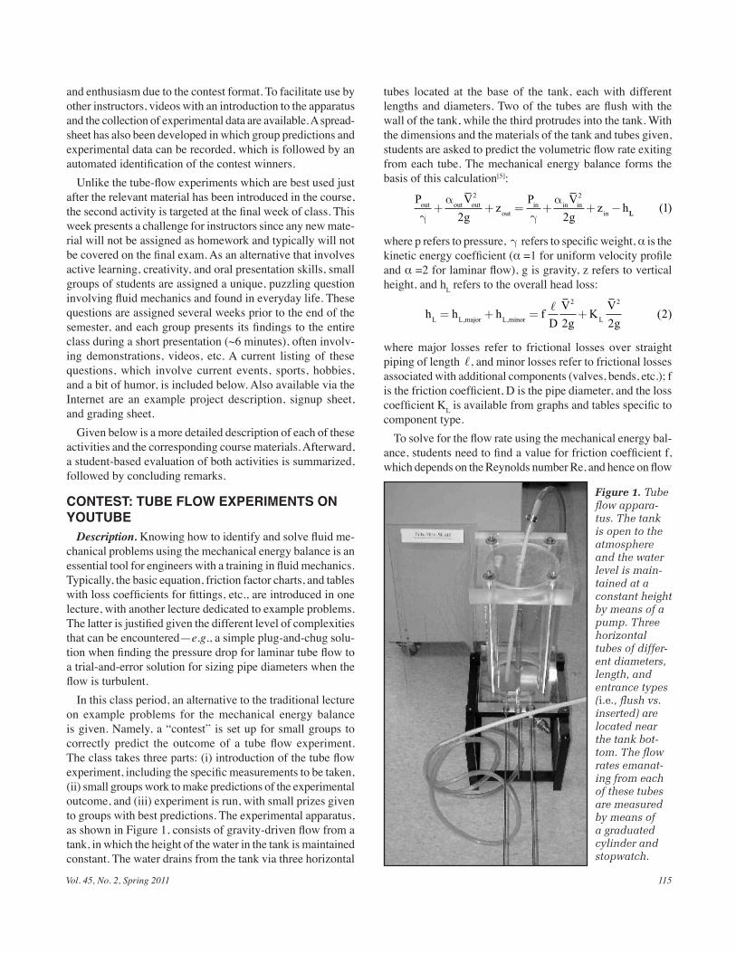
Vol. 45, No. 2, Spring 2011 115
and enthusiasm due to the contest format. To facilitate use by other instructors, videos with an introduction to the apparatus and the collection of experimental data are available. A spread-sheet has also been developed in which group predictions and experimental data can be recorded, which is followed by an automated identification of the contest winners.
Unlike the tube-flow experiments which are best used just after the relevant material has been introduced in the course, the second activity is targeted at the final week of class. This week presents a challenge for instructors since any new mate-rial will not be assigned as homework and typically will not be covered on the final exam. As an alternative that involves active learning, creativity, and oral presentation skills, small groups of students are assigned a unique, puzzling question involving fluid mechanics and found in everyday life. These questions are assigned several weeks prior to the end of the semester, and each group presents its findings to the entire class during a short presentation (~6 minutes), often involv-ing demonstrations, videos, etc. A current listing of these questions, which involve current events, sports, hobbies, and a bit of humor, is included below. Also available via the Internet are an example project description, signup sheet, and grading sheet.
Given below is a more detailed description of each of these activities and the corresponding course materials. Afterward, a student-based evaluation of both activities is summarized, followed by concluding remarks.
CONTEST: TUBE FLOW EXPERIMENTS ON YOUTUBE
Description. Knowing how to identify and solve fluid me-chanical problems using the mechanical energy balance is an essential tool for engineers with a training in fluid mechanics. Typically, the basic equation, friction factor charts, and tables with loss coefficients for fittings, etc., are introduced in one lecture, with another lecture dedicated to example problems. The latter is justified given the different level of complexities that can be encountered—e.g., a simple plug-and-chug solu-tion when finding the pressure drop for laminar tube flow to a trial-and-error solution for sizing pipe diameters when the flow is turbulent.
In this class period, an alternative to the traditional lecture on example problems for the mechanical energy balance is given. Namely, a “contest” is set up for small groups to correctly predict the outcome of a tube flow experiment. The class takes three parts: (i) introduction of the tube flow experiment, including the specific measurements to be taken, (ii) small groups work to make predictions of the experimental outcome, and (iii) experiment is run, with small prizes given to groups with best predictions. The experimental apparatus, as shown in Figure 1, consists of gravity-driven flow from a tank, in which the height of the water in the tank is maintained constant. The water drains from the tank via three horizontal
tubes located at the base of the tank, each with different lengths and diameters. Two of the tubes are flush with the wall of the tank, while the third protrudes into the tank. With the dimensions and the materials of the tank and tubes given, students are asked to predict the volumetric flow rate exiting from each tube. The mechanical energy balance forms the basis of this calculation[5]:
P Vg
zP V
gz hout out out
outin in in
inγα
γα
+ + = + + −2 2
2 2 LL ( )1
where p refers to pressure, γ refers to specific weight, α is the kinetic energy coefficient (α =1 for uniform velocity profile and α =2 for laminar flow), g is gravity, z refers to vertical height, and hL refers to the overall head loss:
h h h fDVg
KVgL L major L L= + = +, , ( )minor
� 2 2
2 22
where major losses refer to frictional losses over straight piping of length �, and minor losses refer to frictional losses associated with additional components (valves, bends, etc.); f is the friction coefficient, D is the pipe diameter, and the loss coefficient KL is available from graphs and tables specific to component type.
To solve for the flow rate using the mechanical energy bal-ance, students need to find a value for friction coefficient f, which depends on the Reynolds number Re, and hence on flow
Figure 1. Tube flow appara-tus. The tank is open to the atmosphere and the water level is main-tained at a constant height by means of a pump. Three horizontal tubes of differ-ent diameters, length, and entrance types (i.e., flush vs. inserted) are located near the tank bot-tom. The flow rates emanat-ing from each of these tubes are measured by means of a graduated cylinder and stopwatch.
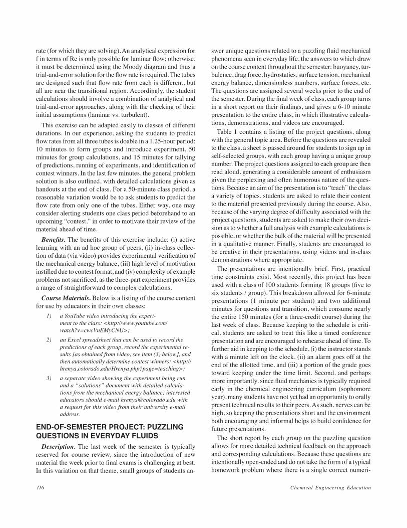
Chemical Engineering Education116
rate (for which they are solving). An analytical expression for f in terms of Re is only possible for laminar flow; otherwise, it must be determined using the Moody diagram and thus a trial-and-error solution for the flow rate is required. The tubes are designed such that flow rate from each is different, but all are near the transitional region. Accordingly, the student calculations should involve a combination of analytical and trial-and-error approaches, along with the checking of their initial assumptions (laminar vs. turbulent).
This exercise can be adapted easily to classes of different durations. In our experience, asking the students to predict flow rates from all three tubes is doable in a 1.25-hour period: 10 minutes to form groups and introduce experiment, 50 minutes for group calculations, and 15 minutes for tallying of predictions, running of experiments, and identification of contest winners. In the last few minutes, the general problem solution is also outlined, with detailed calculations given as handouts at the end of class. For a 50-minute class period, a reasonable variation would be to ask students to predict the flow rate from only one of the tubes. Either way, one may consider alerting students one class period beforehand to an upcoming “contest,” in order to motivate their review of the material ahead of time.
Benefits. The benefits of this exercise include: (i) active learning with an ad hoc group of peers, (ii) in-class collec-tion of data (via video) provides experimental verification of the mechanical energy balance, (iii) high level of motivation instilled due to contest format, and (iv) complexity of example problems not sacrificed, as the three-part experiment provides a range of straightforward to complex calculations.
Course Materials. Below is a listing of the course content for use by educators in their own classes:
1) a YouTube video introducing the experi-ment to the class: <http://www.youtube.com/watch?v=cwcVnEMyCNU>;
2) an Excel spreadsheet that can be used to record the predictions of each group, record the experimental re-sults [as obtained from video, see item (3) below], and then automatically determine contest winners: <http://hrenya.colorado.edu/Hrenya.php?page=teaching>;
3) a separate video showing the experiment being run and a “solutions” document with detailed calcula-tions from the mechanical energy balance; interested educators should e-mail [email protected] with a request for this video from their university e-mail address.
END-OF-SEMESTER PROJECT: PUZZLING QUESTIONS IN EVERYDAY FLUIDS
Description. The last week of the semester is typically reserved for course review, since the introduction of new material the week prior to final exams is challenging at best. In this variation on that theme, small groups of students an-
swer unique questions related to a puzzling fluid mechanical phenomena seen in everyday life, the answers to which draw on the course content throughout the semester: buoyancy, tur-bulence, drag force, hydrostatics, surface tension, mechanical energy balance, dimensionless numbers, surface forces, etc. The questions are assigned several weeks prior to the end of the semester. During the final week of class, each group turns in a short report on their findings, and gives a 6-10 minute presentation to the entire class, in which illustrative calcula-tions, demonstrations, and videos are encouraged.
Table 1 contains a listing of the project questions, along with the general topic area. Before the questions are revealed to the class, a sheet is passed around for students to sign up in self-selected groups, with each group having a unique group number. The project questions assigned to each group are then read aloud, generating a considerable amount of enthusiasm given the perplexing and often humorous nature of the ques-tions. Because an aim of the presentation is to “teach” the class a variety of topics, students are asked to relate their content to the material presented previously during the course. Also, because of the varying degree of difficulty associated with the project questions, students are asked to make their own deci-sion as to whether a full analysis with example calculations is possible, or whether the bulk of the material will be presented in a qualitative manner. Finally, students are encouraged to be creative in their presentations, using videos and in-class demonstrations where appropriate.
The presentations are intentionally brief. First, practical time constraints exist. Most recently, this project has been used with a class of 100 students forming 18 groups (five to six students / group). This breakdown allowed for 6-minute presentations (1 minute per student) and two additional minutes for questions and transition, which consume nearly the entire 150 minutes (for a three-credit course) during the last week of class. Because keeping to the schedule is criti-cal, students are asked to treat this like a timed conference presentation and are encouraged to rehearse ahead of time. To further aid in keeping to the schedule, (i) the instructor stands with a minute left on the clock, (ii) an alarm goes off at the end of the allotted time, and (iii) a portion of the grade goes toward keeping under the time limit. Second, and perhaps more importantly, since fluid mechanics is typically required early in the chemical engineering curriculum (sophomore year), many students have not yet had an opportunity to orally present technical results to their peers. As such, nerves can be high, so keeping the presentations short and the environment both encouraging and informal helps to build confidence for future presentations.
The short report by each group on the puzzling question allows for more detailed technical feedback on the approach and corresponding calculations. Because these questions are intentionally open-ended and do not take the form of a typical homework problem where there is a single correct numeri-
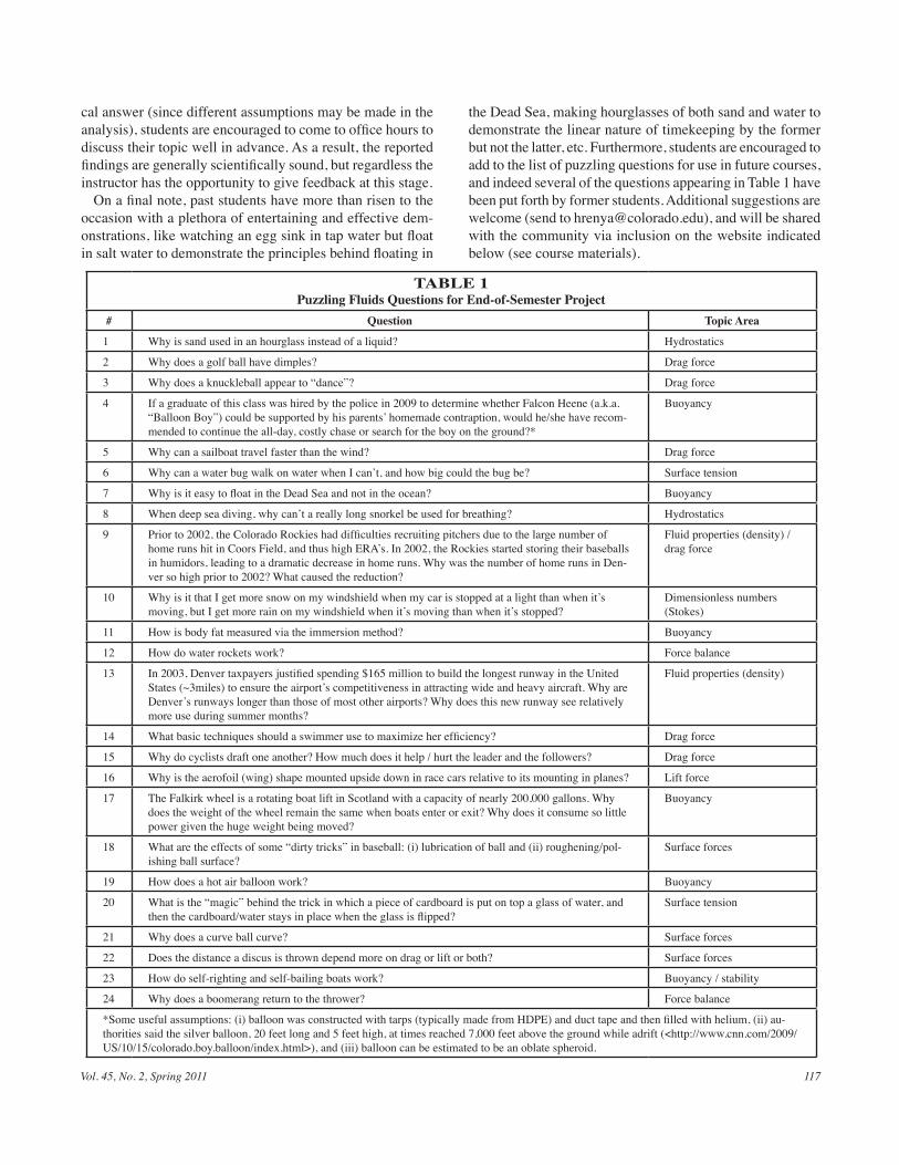
Vol. 45, No. 2, Spring 2011 117
TABLE 1Puzzling Fluids Questions for End-of-Semester Project
# Question Topic Area
1 Why is sand used in an hourglass instead of a liquid? Hydrostatics
2 Why does a golf ball have dimples? Drag force
3 Why does a knuckleball appear to “dance”? Drag force
4 If a graduate of this class was hired by the police in 2009 to determine whether Falcon Heene (a.k.a. “Balloon Boy”) could be supported by his parents’ homemade contraption, would he/she have recom-mended to continue the all-day, costly chase or search for the boy on the ground?*
Buoyancy
5 Why can a sailboat travel faster than the wind? Drag force
6 Why can a water bug walk on water when I can’t, and how big could the bug be? Surface tension
7 Why is it easy to float in the Dead Sea and not in the ocean? Buoyancy
8 When deep sea diving, why can’t a really long snorkel be used for breathing? Hydrostatics
9 Prior to 2002, the Colorado Rockies had difficulties recruiting pitchers due to the large number of home runs hit in Coors Field, and thus high ERA’s. In 2002, the Rockies started storing their baseballs in humidors, leading to a dramatic decrease in home runs. Why was the number of home runs in Den-ver so high prior to 2002? What caused the reduction?
Fluid properties (density) / drag force
10 Why is it that I get more snow on my windshield when my car is stopped at a light than when it’s moving, but I get more rain on my windshield when it’s moving than when it’s stopped?
Dimensionless numbers (Stokes)
11 How is body fat measured via the immersion method? Buoyancy
12 How do water rockets work? Force balance
13 In 2003, Denver taxpayers justified spending $165 million to build the longest runway in the United States (~3miles) to ensure the airport’s competitiveness in attracting wide and heavy aircraft. Why are Denver’s runways longer than those of most other airports? Why does this new runway see relatively more use during summer months?
Fluid properties (density)
14 What basic techniques should a swimmer use to maximize her efficiency? Drag force
15 Why do cyclists draft one another? How much does it help / hurt the leader and the followers? Drag force
16 Why is the aerofoil (wing) shape mounted upside down in race cars relative to its mounting in planes? Lift force
17 The Falkirk wheel is a rotating boat lift in Scotland with a capacity of nearly 200,000 gallons. Why does the weight of the wheel remain the same when boats enter or exit? Why does it consume so little power given the huge weight being moved?
Buoyancy
18 What are the effects of some “dirty tricks” in baseball: (i) lubrication of ball and (ii) roughening/pol-ishing ball surface?
Surface forces
19 How does a hot air balloon work? Buoyancy
20 What is the “magic” behind the trick in which a piece of cardboard is put on top a glass of water, and then the cardboard/water stays in place when the glass is flipped?
Surface tension
21 Why does a curve ball curve? Surface forces
22 Does the distance a discus is thrown depend more on drag or lift or both? Surface forces
23 How do self-righting and self-bailing boats work? Buoyancy / stability
24 Why does a boomerang return to the thrower? Force balance
*Some useful assumptions: (i) balloon was constructed with tarps (typically made from HDPE) and duct tape and then filled with helium, (ii) au-thorities said the silver balloon, 20 feet long and 5 feet high, at times reached 7,000 feet above the ground while adrift (<http://www.cnn.com/2009/US/10/15/colorado.boy.balloon/index.html>), and (iii) balloon can be estimated to be an oblate spheroid.
cal answer (since different assumptions may be made in the analysis), students are encouraged to come to office hours to discuss their topic well in advance. As a result, the reported findings are generally scientifically sound, but regardless the instructor has the opportunity to give feedback at this stage.
On a final note, past students have more than risen to the occasion with a plethora of entertaining and effective dem-onstrations, like watching an egg sink in tap water but float in salt water to demonstrate the principles behind floating in
the Dead Sea, making hourglasses of both sand and water to demonstrate the linear nature of timekeeping by the former but not the latter, etc. Furthermore, students are encouraged to add to the list of puzzling questions for use in future courses, and indeed several of the questions appearing in Table 1 have been put forth by former students. Additional suggestions are welcome (send to [email protected]), and will be shared with the community via inclusion on the website indicated below (see course materials).
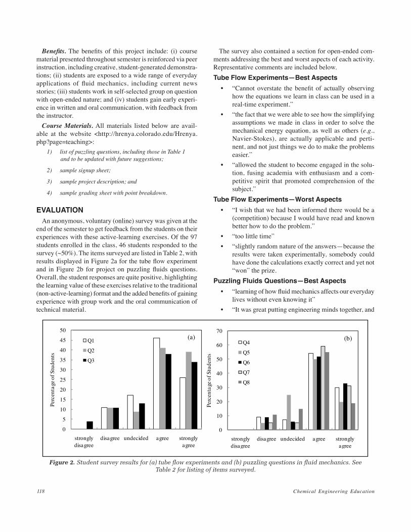
Chemical Engineering Education118
Benefits. The benefits of this project include: (i) course material presented throughout semester is reinforced via peer instruction, including creative, student-generated demonstra-tions; (ii) students are exposed to a wide range of everyday applications of fluid mechanics, including current news stories; (iii) students work in self-selected group on question with open-ended nature; and (iv) students gain early experi-ence in written and oral communication, with feedback from the instructor.
Course Materials. All materials listed below are avail-able at the website <http://hrenya.colorado.edu/Hrenya.php?page=teaching>:
1) list of puzzling questions, including those in Table 1 and to be updated with future suggestions;
2) sample signup sheet;
3) sample project description; and
4) sample grading sheet with point breakdown.
EVALUATIONAn anonymous, voluntary (online) survey was given at the
end of the semester to get feedback from the students on their experiences with these active-learning exercises. Of the 97 students enrolled in the class, 46 students responded to the survey (~50%). The items surveyed are listed in Table 2, with results displayed in Figure 2a for the tube flow experiment and in Figure 2b for project on puzzling fluids questions. Overall, the student responses are quite positive, highlighting the learning value of these exercises relative to the traditional (non-active-learning) format and the added benefits of gaining experience with group work and the oral communication of technical material.
The survey also contained a section for open-ended com-ments addressing the best and worst aspects of each activity. Representative comments are included below.Tube Flow Experiments—Best Aspects
• “Cannot overstate the benefit of actually observing how the equations we learn in class can be used in a real-time experiment.”
• “the fact that we were able to see how the simplifying assumptions we made in class in order to solve the mechanical energy equation, as well as others (e.g., Navier-Stokes), are actually applicable and perti-nent, and not just things we do to make the problems easier.”
• “allowed the student to become engaged in the solu-tion, fusing academia with enthusiasm and a com-petitive spirit that promoted comprehension of the subject.”
Tube Flow Experiments—Worst Aspects• “I wish that we had been informed there would be a
(competition) because I would have read and known better how to do the problem.”
• “too little time”• “slightly random nature of the answers—because the
results were taken experimentally, somebody could have done the calculations exactly correct and yet not “won” the prize.
Puzzling Fluids Questions—Best Aspects• “learning of how fluid mechanics affects our everyday
lives without even knowing it”• “It was great putting engineering minds together, and
Figure 2. Student survey results for (a) tube flow experiments and (b) puzzling questions in fluid mechanics. See Table 2 for listing of items surveyed.
0
5
10
15
20
25
30
35
40
45
50
strongly disagree
disagree undecided agree strongly agree
Perc
enta
ge o
f Stu
dent
s
Q1
Q2
Q3
(a)
0
10
20
30
40
50
60
70
strongly disagree
disagree undecided agree strongly agree
Perc
enta
ge o
f Stu
dent
s
Q4
Q5
Q6
Q7
Q8
(b)
Vol. 45, No. 2, Spring 2011 119
hearing each person’s strong points about the particular problem. Groups can have a great deal of creativity with a cumulative effect from each individual.”
• “learning about not only our project but other projects”
• “The projects were just plain fun.”Puzzling Fluids Questions—Worst Aspects
• “trying to get everyone to agree on ideas.”• “difficult to try to explain the concept and for everyone
to talk and still keep it under 6 minutes”• “having to talk in front of our peers (it was scary!)”• “not all of the groups had applied fluids equations in
an understandable manner”
CONCLUDING REMARKSIn this work, two active-learning exercises appropriate for
an undergraduate course in fluid mechanics are presented. Based on firsthand experience using these exercises with hundreds of students, it is found that the exercises effec-tively promote student interaction, give rise to thoughtful student questions, serve as good learning tools, and last but not least, add quite a bit of enjoyment to the class period for all involved.
ACKNOWLEDGMENTSThe author would like to express thanks to Will Brewer,
who prepared the sample calculations and YouTube video. The author is also indebted to the students, teaching assistants, and colleagues who have contributed to the list of puzzling fluid-mechanics questions over the years. Funding support for this work was provided by the National Science Foundation (CBET-0658903).
REFERENCES 1. Prince, M., “Does Active Learning Work? A Review of the Research,”
J. Eng. Ed., 93, 223-231 (2004) 2. Smith, K.A., S.D. Sheppard, D. W. Johnson, and R.T. Johnson, “Peda-
gogies of Engagement: Classroom-Based Practices,” J. Eng. Ed., 94, 87-101 (2005)
3. Felder, R., D. Woods, J. Stice, and A. Rugarcia, “The Future of En-gineering Education: II. Teaching Methods That Work,” Chem. Eng. Ed., 34, 26-39 (2000)
4. Ford, L.P. , “Water Day: An Experiential Lecture for Fluid Mechanics,” Chem. Eng. Ed., 37, (2003)
5. Munson, B.R., D.F. Young, T.H. Okiishi, and W.W. Huebsch, Funda-mentals of Fluid Mechanics, Wiley, New York (2009) p
TABLE 2Items Used in Student Survey
See Figure 2 for responses.# Item
Tube Flow Demonstration
Q1 This class period was a more valuable learning experi-ence than a lecture with example problems.
Q2 The contest format (i.e., prizes for winners) provided more focus and energy on the task than would have been present otherwise.
Q3 This class period was the most fun of the semester.
Puzzling Questions in Fluid Mechanics
Q4 Attending these presentations and working on my own project illustrated the everyday relevance of fluid mechanics better than other means used during the se-mester (examples during lecture, homework problems, etc.).
Q5 Attending these presentations strengthened my under-standing of basic fluid mechanical principles.
Q6 This project provided a good learning experience about working in teams.
Q7 This project provided a good learning experience for the oral communication of scientific ideas to peers.
Q8 This project provided a good learning experience in written communication of scientific ideas.
Chemical Engineering Education120
The advantages of the semi-batch reactor (SBR) are exploited in several industrial reactor applications. For example, in the reaction of a gas with a liquid (e.g.,
ozonation of industrial wastewater to remove dyes[1]), the gas is continuously bubbled through the batch liquid. Conversely, a gaseous product can be continuously removed from a liquid system (e.g., CO2 in fermentation). The slow addition of one reactant into another assists in the control of a strong exotherm in the SBR, such as in polymerization reactors (e.g., nylon[2] and polypropylene[3]). Polymer molecular weight distributions can be controlled by careful addition of the monomer (e.g., styrene-butadiene rubber[4]). The SBR can be used to maxi-mize selectivity, especially where byproducts or competing reactions are an issue (e.g., substituted alkyl phenols[5]).
In spite of its industrial use, the SBR is often ignored in undergraduate reactor engineering classes. Still, the SBR offers a useful opportunity to combine both batch and flow concepts. Haji and Erkey[6] present an SBR experiment with the exothermic hydrolysis of acetic anhydride. In-situ Fourier transfer infrared spectroscopy is used for monitoring spe-cies of interest vs. time. Kinetic analyses are subsequently performed.
In this paper, an SBR is used to process the simple reac-tion between sodium hypochlorite and hydrogen peroxide. Inexpensive household bleach and pharmaceutical hydrogen peroxide solution serve as the convenient reactants. Product molecular oxygen is monitored through a rotameter. The over-all change in solution conductivity is metered with a conduc-tivity probe. The reaction exothermicity is monitored through a reactor thermocouple. The elegant model analyses combine reaction kinetics with species and energy balances.
REACTION AND KINETICS The reaction used in this experiment is inspired by Shams
El Din and Mohammed,[7] who studied the kinetics of this reaction as a means to remove residual bleach from water purification equipment.
H2O2(aq) + NaOCl(aq) → H2O(l) + NaCl(aq) + O2(g)
A + B → R + S + T
A SEMI-BATCH REACTOR EXPERIMENT for the Undergraduate Laboratory
ChE laboratory
Mario Derevjanik, Solmaz Badri, and Robert Barat New Jersey Institute of Technology • Newark, NJ 0102
Solmaz Badri was born in Teh-ran, Iran, and came to the United States after completing high school. She joined NJIT and graduated in 2009, majoring in chemical engineering. She is now living in New York City, married to a physician, and working as an individual contractor. She dedicates her work and research to her newborn son, Amin Zamanian.
Mario Derevjanik graduated from NJIT with a B.S. in chemical engineering in 2008. During his undergraduate career, Mario assisted Dr. Barat in developing new student experiments. Mario is working as a chemical engineer for ConSerTech, a small environmental consulting company. His cur-rent responsibilities, including VOC monitor-ing, are at the Conoco-Phillips refinery in
Linden, NJ.
© Copyright ChE Division of ASEE 2011
The letters representing the species are shown in corre-sponding order. The reported rate expression for the disap-pearance of A is second order:
− = =− = = ( )r kC C r r rA A B B S T 1
where ri = reaction rate of species i, k = reaction rate con-stant, and Ci = molar concentration of i. Because the reaction evolves gaseous O2 rather rapidly, it is preferable to run it in a semi-batch reactor. To start, a batch vessel contains hydrogen peroxide (H2O2 – species A) in a water solution. The aqueous solution of sodium hypochlorite (NaOCl – species B) is fed slowly over time at a constant rate. As shown above, species S and T are NaCl and O2, respectively.
Robert Barat is currently a professor of chemical engineering at NJIT, where he has been a member of the faculty since 1990. He completed his Ph.D. in chemical engineering at MIT in 1990. His research has been in com-bustion, reactor engineering, environmental monitoring, applied optics, and is currently in applied catalysis. He is also the faculty coordinator for the chemical engineering laboratories at NJIT.
Vol. 45, No. 2, Spring 2011 121
REACTOR SPECIES BALANCES A semi-batch design equation applies for B:
F r VdNdtB BB+ = ( )2
where FB = molar flow rate inlet to the batch, V = batch liquid volume, and Ni = moles of i in the batch. A simple batch design equation applies for A:
r VdNdtAA= ( )3
The inlet molar flow rate of B can be written in more con-venient volumetric terms:
Fv fWBB B B
B
= ( )ρ4
where vB = volumetric feed rate of B, ρB = bleach mass den-sity, fB = mass fraction of species B in the feed bleach solution, and WB = molecular weight of B. Since Ni = CiV, and V = f(t) in the most general semi-batch case, Eq. (3) becomes:
rCVdVdt
dCdtA
A A− = ( )5
and Eq. (2) becomes:
FV
rCVdVdt
dCdt
BB
B B+ − = ( )6
The rate of change of the volume is accounted for with a transient mass balance:
vd VdtB Bρρ
=( ) ( )7
where ρ =mass density of batch solution. It can be rea-sonably assumed ρ is constant; then, Eq. (7) reduces to:
v dVdtB
Bρρ= ( )8
The volumetric feed rate of B is set at a constant value by the user in the experiment.
Eqs. (1), (4)-(6), and (8) form a partial system that will be solved simultaneously. The system is integrated from t = 0 (when the reactant B solution flow begins) to whenever the peroxide feed is ended by the user.
EVOLUTION OF O2 Assuming that the bleach solution mixes thoroughly into
the peroxide solution, the reaction mixture will likely saturate with O2 very rapidly. We can assume that the O2 evolution rate is approximately the same as the reaction rate, and is given by:
F r VT T≈ ( )9
The Ideal Gas Law can be used to convert FT to a volu-metric rate.
r VRTP
vT s
sT≈ ( )10
where Ts, Ps represent standard temperature and pressure conditions (298 K, 1 atm), respectively, and R = ideal gas constant (0.0821 liter-atm/mole-K). Eq. (10) can be added to the set of equations to be solved. The volumetric rate of evolved O2 is one of three possible sources of data in this experiment. The rate rT is obtained from Eq. (1).
CONDUCTIVITY CHANGE AND CHLORIDE IONThe conductivity of the solution is a weighted sum of the
contributions of the ionic species, including NaOCl as the active ingredient, a small amount of NaOH to help prevent degradation of NaOCl to release Cl2, and residual NaCl from the bleach manufacturing process. We assume that CNaOCl in the SBR is very small, and insignificantly contributes to the solution conductivity. Subsequent SBR modeling supports this claim. The batch solution conductivity can be estimated as:
C c C c C c C Cond Conii
i NaCl NaCl NaOH NaOH NaCl≈ ≡ +∑ = + ddNaOH
11( )where C = solution conductivity, ci = effective molar con-ductivity of species i, Ci = molar concentration of i, and Condi = contribution of i to the total conductivity.
Accounting for the contribution of NaCl to the solution conductivity requires a species balance, including the pres-ence of NaCl in the bleach feed:
FV
rCVdVdt
dCdt
ss
s s+ − = ( )12
The inlet molar flow rate of S can be written in more con-venient volumetric terms:
Fv fWSB B S
S
= ( )ρ13
where fS = mass fraction of NaCl in the feed bleach solution. Molar conductivity data for NaCl aqueous solutions are available[8] over the temperature range of interest to yield a relationship valid up to 0.85 molar concentration:
Λ
ΛSO
c c
SO
T T= + +0 0117 1 3737 51 6652. . .
( in mS/cm/mmolar, temperature T in C)c�
The contribution of the NaOH to the solution conductiv-ity is:
Cond CS SO
S= ( )Λ 14
Accounting for the contribution of NaOH to the solution
Chemical Engineering Education122
conductivity requires a non-reactive species balance. Repre-senting NaOH as the inert I, the balance is:
FV
CV
dVdt
dCdt
I I I− = ( )15
The inlet molar flow rate of I can be written in more con-venient volumetric terms:
Fv f
WIB B I
I
= ( )ρ16
where fI = mass fraction of NaOH in the feed bleach solution. Molar conductivity ΛI
O data for NaOH aqueous solutions are available[11] over the temperature range of interest to yield a relationship valid up to 0.3 molar concentration:
Λ
ΛIO
c c
IO
T T=− + +0 0241 5 0658 111 132. . .
( in mS/cm//molar, temperature T in C)c�
The contribution of the NaOH to the solution conductiv-ity is:
Cond CI IO
I= ( )Λ 17
ENERGY BALANCE The energy balance should reflect the configuration of the
reactor vessel. In a typical experiment, the liquid is in contact with stainless steel walls and internal components (e.g., agi-tator, probes). An air-filled jacket surrounds the walls. Heat losses to this metal must be considered. A simple heat loss calibration was performed wherein an electric immersion heater of known wattage was placed into the vessel filled with water covering the metal parts. A simple heat balance of this calibration is:
dTdt
Qm c m c
ah
w pw m pm
=+
( )18
where Qh = electrical heating rate; mw and mm = masses of water and metal parts, respectively; and cpw and cpm = mass-based specific heats of water and metal, respectively. A suc-cessful linear regression of the measured temperature vs. time, according to the integrated form of Eq. (18a), yielded a heat loss calibration of mmcpm = 1284 cal/ ˚C.
It can be shown, consistent with Fogler and Gurmen,[9] that the reactor energy balance is:
dTdt
dT V P dVdt
F c r H
m c
ji
pT
T
A r
m
o j
f
A
=
− + ( )( )+∑ ∫ − −∆
ppm p jj
V c Cj
+ ∑
( )18b
where T = reactor temperature, cpj = molar heat capacity of
species j, Cj = molar concentration of j inside the reactor, Fjo = molar feed rate of j, Tf = feed temperature, ΔHrA = heat of reaction per mole of A, and P = system pressure. The final term in the numerator is included since the fluid volume is not constant. It is small compared to the other terms, however, and can be neglected. Selected terms are now examined.
c CcMp j
j
p
j∑ = ( )
ρ19
where cp and M are the mean molar heat capacity and molecu-lar weight, respectively, of the solution. As an approximation due to the high degree of dilution, the properties of the solvent water can be used. If the mass-based value is used for cp , M is not needed.
F c dTv c
MT Tj
jp
T
TB B p
BBo j
f
B∑ ∫ ≈ −( ) ( )ρ
20
where TB, MB, and cpB = temperature, average molecular weight, and mean heat capacity (mole-based), respectively, of the feed bleach. If the mass-based value is used for cpB, MB is not needed.
The standard heat of reaction (-37.2 kcal/mole at 25 ˚C for the reaction as written earlier) is assumed to be independent of temperature, especially in consideration of the limited temperature range of the experiment.
The energy balance in the form used for data modeling is now written as:
dTdt
v c T T V r H
m c VcB B p B A r
m pm p
B A=− −( )+ −( ) −∆( )
+
ρ
ρ
( )21
EXPERIMENTAL CONSIDERATIONS Figure 1 illustrates the basic configuration of the current
experimental system. An agitated reactor vessel is used. The
Data PC
Bleachconductivityprobe
Temp
thermocouple
O2 product
Figure 1. Schematic of the semi-batch reactor experiment.
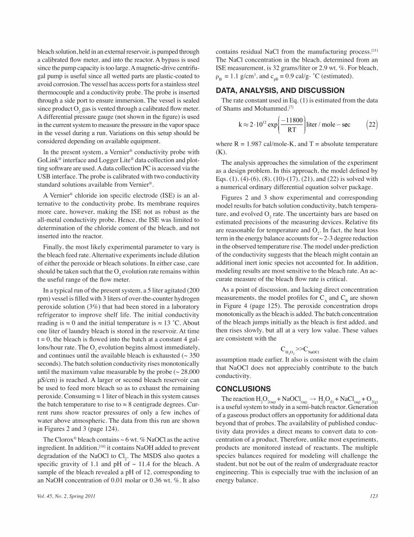
Vol. 45, No. 2, Spring 2011 123
bleach solution, held in an external reservoir, is pumped through a calibrated flow meter, and into the reactor. A bypass is used since the pump capacity is too large. A magnetic-drive centrifu-gal pump is useful since all wetted parts are plastic-coated to avoid corrosion. The vessel has access ports for a stainless steel thermocouple and a conductivity probe. The probe is inserted through a side port to ensure immersion. The vessel is sealed since product O2 gas is vented through a calibrated flow meter. A differential pressure gauge (not shown in the figure) is used in the current system to measure the pressure in the vapor space in the vessel during a run. Variations on this setup should be considered depending on available equipment.
In the present system, a Vernier® conductivity probe with GoLink® interface and Logger Lite® data collection and plot-ting software are used. A data collection PC is accessed via the USB interface. The probe is calibrated with two conductivity standard solutions available from Vernier®.
A Vernier® chloride ion specific electrode (ISE) is an al-ternative to the conductivity probe. Its membrane requires more care, however, making the ISE not as robust as the all-metal conductivity probe. Hence, the ISE was limited to determination of the chloride content of the bleach, and not inserted into the reactor.
Finally, the most likely experimental parameter to vary is the bleach feed rate. Alternative experiments include dilution of either the peroxide or bleach solutions. In either case, care should be taken such that the O2 evolution rate remains within the useful range of the flow meter.
In a typical run of the present system, a 5 liter agitated (200 rpm) vessel is filled with 3 liters of over-the-counter hydrogen peroxide solution (3%) that had been stored in a laboratory refrigerator to improve shelf life. The initial conductivity reading is ≈ 0 and the initial temperature is ≈ 13 ˚C. About one liter of laundry bleach is stored in the reservoir. At time t = 0, the bleach is flowed into the batch at a constant 4 gal-lons/hour rate. The O2 evolution begins almost immediately, and continues until the available bleach is exhausted (~ 350 seconds). The batch solution conductivity rises monotonically until the maximum value measurable by the probe (~ 28,000 μS/cm) is reached. A larger or second bleach reservoir can be used to feed more bleach so as to exhaust the remaining peroxide. Consuming ≈ 1 liter of bleach in this system causes the batch temperature to rise to ≈ 8 centigrade degrees. Cur-rent runs show reactor pressures of only a few inches of water above atmospheric. The data from this run are shown in Figures 2 and 3 (page 124).
The Clorox® bleach contains ~ 6 wt. % NaOCl as the active ingredient. In addition,[10] it contains NaOH added to prevent degradation of the NaOCl to Cl2. The MSDS also quotes a specific gravity of 1.1 and pH of ~ 11.4 for the bleach. A sample of the bleach revealed a pH of 12, corresponding to an NaOH concentration of 0.01 molar or 0.36 wt. %. It also
contains residual NaCl from the manufacturing process.[11] The NaCl concentration in the bleach, determined from an ISE measurement, is 32 grams/liter or 2.9 wt. %. For bleach, ρB = 1.1 g/cm3, and cpB = 0.9 cal/g- ˚C (estimated).
DATA, ANALYSIS, AND DISCUSSION The rate constant used in Eq. (1) is estimated from the data
of Shams and Mohammed.[7]
kRT
liter mole≈ ⋅−
−2 10 1180012 exp / seec 22( )
where R = 1.987 cal/mole-K, and T = absolute temperature (K).
The analysis approaches the simulation of the experiment as a design problem. In this approach, the model defined by Eqs. (1), (4)-(6), (8), (10)-(17), (21), and (22) is solved with a numerical ordinary differential equation solver package.
Figures 2 and 3 show experimental and corresponding model results for batch solution conductivity, batch tempera-ture, and evolved O2 rate. The uncertainty bars are based on estimated precisions of the measuring devices. Relative fits are reasonable for temperature and O2. In fact, the heat loss term in the energy balance accounts for ~ 2-3 degree reduction in the observed temperature rise. The model under-prediction of the conductivity suggests that the bleach might contain an additional inert ionic species not accounted for. In addition, modeling results are most sensitive to the bleach rate. An ac-curate measure of the bleach flow rate is critical.
As a point of discussion, and lacking direct concentration measurements, the model profiles for CA and CB are shown in Figure 4 (page 125). The peroxide concentration drops monotonically as the bleach is added. The batch concentration of the bleach jumps initially as the bleach is first added, and then rises slowly, but all at a very low value. These values are consistent with the
CH O2 2>>CNaOCl
assumption made earlier. It also is consistent with the claim that NaOCl does not appreciably contribute to the batch conductivity.
CONCLUSIONS The reaction H2O2(aq) + NaOCl(aq) → H2O(l) + NaCl(aq) + O2(g)
is a useful system to study in a semi-batch reactor. Generation of a gaseous product offers an opportunity for additional data beyond that of probes. The availability of published conduc-tivity data provides a direct means to convert data to con-centration of a product. Therefore, unlike most experiments, products are monitored instead of reactants. The multiple species balances required for modeling will challenge the student, but not be out of the realm of undergraduate reactor engineering. This is especially true with the inclusion of an energy balance.
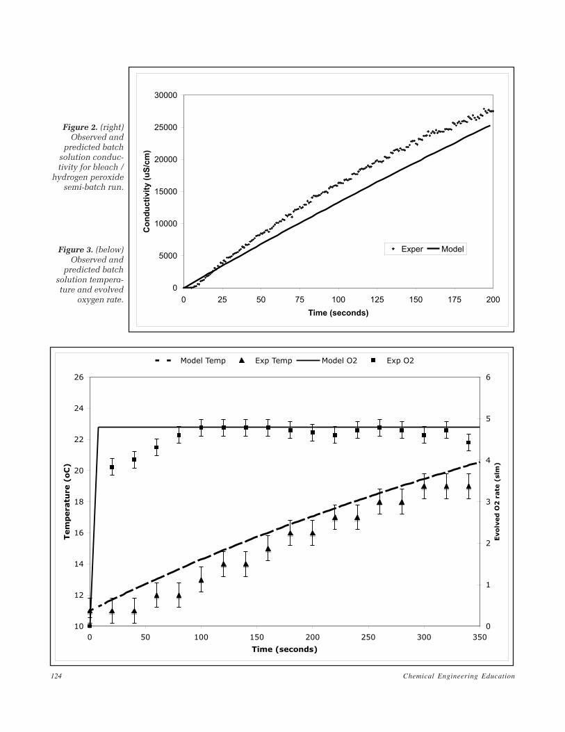
Chemical Engineering Education124
0
5000
10000
15000
20000
25000
30000
0 25 50 75 100 125 150 175 200
Time (seconds)
Co
nd
ucti
vit
y (
uS
/cm
)
Exper Model
10
12
14
16
18
20
22
24
26
0 50 100 150 200 250 300 350
Time (seconds)
Tem
peratu
re (
oC
)
0
1
2
3
4
5
6
Evo
lved
O2
rate
(slm
)
Model Temp Exp Temp Model O2 Exp O2
Figure 2. (right) Observed and
predicted batch solution conduc-tivity for bleach /
hydrogen peroxide semi-batch run.
Figure 3. (below) Observed and
predicted batch solution tempera-ture and evolved
oxygen rate.
Vol. 45, No. 2, Spring 2011 125
REFERENCES 1. Gharbani, P., S.M. Tabatabaii, and A. Mehrizad, “Removal of Congo
Red from Textile Wastewater by Ozonation,” Int. J. of Environmental Science and Technology, 5(4), 495 (2008)
2. Wakabayashi, C., M. Embiruçu, C. Fontes, and R. Kalid, “Fuzzy Control of a Nylon Polymerization Semi-Batch Reactor,” Fuzzy Sets and Systems, 160(4), 537 (2009)
3. Seki, H., M. Ogawa, and M. Ohshima, “Industrial Application of a Nonlinear Predictive Control to a Semi-Batch Polymerization Reactor,” in Advance Control of Chemical Processes, L.T. Biegler, A. Brambilla, and G. Marchetti (eds.), Proceedings of the IFAC Symposium, Pisa, Italy 2000, 2, 539-544 (2001)
4. Yabuki, Y., and J.F. MacGregor, “Product Quality Control in Semi-batch Reactors Using Midcourse Correction Policies,” Industrial & Engineering Chemistry Research, 36(4), 1268 (1997)
5. Lehtonen, J., T. Salmi, A. Vuori, and H. Haario, “Optimization of the Reaction Conditions for Complex Kinetics in a Semibatch Reactor,”
Ind. Eng. Chem. Res., 36(12), 5196 (1997) 6. Haji, S., and C. Erkey, “Kinetics of Hydrolysis of Acetic Anhydride
by In-Situ FTIR Spectroscopy: An Experiment for the Undergraduate Laboratory,” Chem. Eng. Ed., 39(1), 56 (2005)
7. Shams El Din, A.M., and R.A. Mohammed,, “Kinetics of the Reaction Between hydrogen Peroxide and Hypochlorite,” Desalination, 115, 145-153 (1998)
8. Landolt, H., and R. Bornstein, Zahlenwerte und Funktionen aus Natur-wissenschaften und Technik., K.H. Hellwege (ed.), Volume 2, Part. Volume 6, Springer-Verlag, Berlin (1987)—obtained via Honeywell Sensing and Control, Freeport, IL
9. Fogler, H.S., and N.M. Gurmen, Elements of Chemical Reaction Engineering, 4th Ed., Prentice-Hall (2006)
10. <http://www.powellfab.com/technical_information/preview/gen-eral_info_about_so dium_hypo.asp>
11. Clorox® MSDS: <http://www.thecloroxcompany.com/products/msds/> p
Figure 4. Model-based predicted concentrations of species A (H2O2) and B (NaOCl) in the batch.
0.3
0.4
0.5
0.6
0.7
0.8
0.9
0 25 50 75 100 125 150 175 200 225 250 275 300 325 350
Time (seconds)
Batc
h C
on
cen
trati
on
of
H2
O2
(m
ole
s/
lite
r)
0
0.5
1
1.5
2
2.5
3
3.5
4
Batc
h C
on
cen
trati
on
of
NaO
Cl
x 1
0^
11
(m
ole
/li
ter)
CA (H2O2)
CB (NaOCl) x 10^11

Chemical Engineering Education126
Conservation of energy (COE) and conservation of mass (COM)—both are fundamental principles that apply to all aspects of chemical engineering design, analysis,
and education. In most cases, we cannot apply one without consideration of the other. Yet, a third fundamental principle exists that is too often not recognized as on the same level of importance as COE and COM: prevention of serious human injury, major property damage, and environmental harm, which is a primary focus of industrial chemical engineering practice. We choose to call this third principle “conservation of life” (COL), reflecting the need for fundamental awareness and application of process safety and product sustainability concepts in chemical engineering education. COL was first introduced to our knowledge by Lewis DeBlois,[1-3] who was DuPont’s first corporate safety manager and later president of the National Safety Council, when he wrote in 1918:
… safety engineering, with its interests in design, equip-ment, organization, supervision, and education … bears as well a very definite and important relation to all other branches of engineering. This relation is so close, and its need so urgent, that I am convinced that some instruction in the fundamentals of safety engineering should be given a place in the training of every young engineer. He should be taught to think in terms of safety as he now thinks in terms of efficiency. Conservation of life should surely not be rated below the conservation of energy. Yet, few of our technical schools and universities offer instruction in this subject, and the graduates go out to their profession with only vague surmises on “what all this talk on safety is about.”[4]
Much of what DeBlois observed and recommended remains true today, over 90 years later, as identified by the U.S. Chemi-cal Safety Board (CSB) in their report on the T2 Laboratories incident in 2009:
In 2006, the Mary Kay O’Connor Process Safety Center surveyed 180 chemical engineering departments at U.S. universities to determine whether process safety was part of their chemical engineering curricula. Of the universities surveyed, only 11 percent required process safety educa-tion in the core baccalaureate curriculum. An additional 13 percent offered an elective process safety course.[5]
CSB recommended that the American Institute of Chemical Engineers and the Accreditation Board for Engineering and Technology (ABET) work together to improve requirements for chemical engineering education to include greater em-
CONSERVATION OF LIFE as a Unifying Theme for Process Safety
in Chemical Engineering Education
JamES a. KlEin
DuPont, North America OperationsriChard a. daviS
University of Minnesota, Duluth • Duluth, MN
James Klein is a Sr. PSM Competency Consultant, North America PSM Co-lead, at DuPont. He has more than 30 years experience in process engineering, research, operations, and safety. He received his chemical engineering degrees from MIT (B.S.) and Drexel (M.S.) and also has an M.S. in management of technology from the University of Minnesota.
Richard Davis is a professor of chemical engineering at the University of Minnesota, Duluth, where he teaches computational methods, heat and mass transfer, green engineering, and separations. His current research interests include process modeling and simulation applied to energy conversion, pollution control, and environmental management in mineral processing. He received his chemical engineering degrees from Brigham Young University (B.S.) and the University of California, Santa Barbara (Ph.D.).
© Copyright ChE Division of ASEE 2011
ChE curriculum
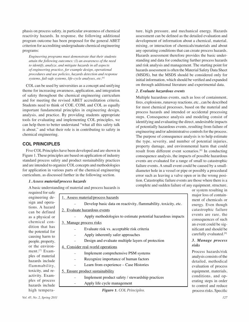
Vol. 45, No. 2, Spring 2011 127
phasis on process safety, in particular awareness of chemical reactivity hazards. In response, the following additional program outcome has been proposed for the general ABET criterion for accrediting undergraduate chemical engineering programs:
Engineering programs must demonstrate that their students attain the following outcomes: (l) an awareness of the need to identify, analyze, and mitigate hazards in all aspects of engineering practice, for example design, operational procedures and use policies, hazards detection and response systems, fail-safe systems, life-cycle analyses, etc.[6]
COL can be used by universities as a concept and unifying theme for increasing awareness, application, and integration of safety throughout the chemical engineering curriculum and for meeting the revised ABET accreditation criteria. Students need to think of COE, COM, and COL as equally important fundamental principles in engineering design, analysis, and practice. By providing students appropriate tools for evaluating and implementing COL principles, we can help them to better understand “what all this safety talk is about,” and what their role is in contributing to safety in chemical engineering.
COL PRINCIPLESFive COL Principles have been developed and are shown in
Figure 1. These principles are based on application of industry standard process safety and product sustainability practices and are intended to organize COL concepts and methodologies for application in various parts of the chemical engineering curriculum, as discussed further in the following section.
1. Assess material/process hazardsA basic understanding of material and process hazards is required for safe engineering de-sign and opera-tions. A hazard can be defined as a physical or chemical con-dition that has the potential for causing harm to people, property, or the environ-ment.[7] Exam-ples of material hazards include f lammabil i ty, toxicity, and re-activity. Exam-ples of process hazards include high tempera-
ture, high pressure, and mechanical energy. Hazards assessment can be defined as the detailed evaluation and development of information about a chemical, material, mixing, or interaction of chemicals/materials and about any operating conditions that can create process hazards. Hazards assessment therefore provides the basic under-standing and data for conducting further process hazards and risk analysis and management. The starting point for hazards assessment is often the Material Safety Data Sheet (MSDS), but the MSDS should be considered only for initial information, which should be verified and expanded on through additional literature and experimental data.2. Evaluate hazardous eventsMultiple hazardous events, such as loss of containment, fires, explosions, runaway reactions, etc., can be described for most chemical processes, based on the material and process hazards and intended or accidental processing steps. Consequence analysis and modeling consist of identifying and evaluating the direct, undesirable impacts of potentially hazardous events, resulting from failure of engineering and/or administrative controls for the process. The purpose of consequence analysis is to help estimate the type, severity, and number of potential injuries, property damage, and environmental harm that could result from different event scenarios.[8] In conducting consequence analysis, the impacts of possible hazardous events are evaluated for a range of small to catastrophic failure events. A small event could be caused by a small-diameter hole in a vessel or pipe or possibly a procedural error such as leaving a valve open or in the wrong posi-tion. Catastrophic failure events are those where there is a complete and sudden failure of any equipment, structure,
or system resulting in major loss of contain-ment of chemicals or energy. Even though catastrophic failure events are rare, the consequences of such an event could be sig-nificant and should be carefully evaluated.[9]
3. Manage process risksProcess hazards/risk analysis consists of the detailed, methodical evaluation of process equipment, materials, conditions, and op-erating steps in order to control and reduce process risks. Specific
1. Assess material/process hazards– Develop basic data on reactivity, flammability, toxicity, etc.
2. Evaluate hazardous events– Apply methodologies to estimate potential hazardous impacts
3. Manage process risks– Evaluate risk vs. acceptable risk criteria– Apply inherently safer approaches– Design and evaluate multiple layers of protection
4. Consider real-world operations– Implement comprehensive PSM systems– Recognize importance of human factors– Learn from experience – Case Histories
5. Ensure product sustainability– Implement product safety / stewardship practices– Apply life cycle management
Figure 1. COL Principles.
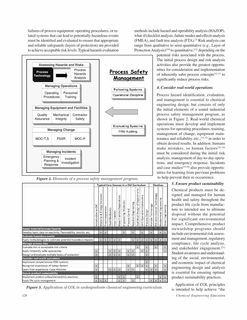
Chemical Engineering Education128
failures of process equipment, operating procedures, or re-lated systems that can lead to potentially hazardous events must be identified and evaluated to ensure that appropriate and reliable safeguards (layers of protection) are provided to achieve acceptable risk levels. Typical hazards evaluation
methods include hazard and operability analysis (HAZOP), what-if/checklist analysis, failure modes and effects analysis (FMEA), and fault tree analysis (FTA).[7] Risk analysis can range from qualitative to semi-quantitative (e.g., Layer of Protection Analysis)[10] to quantitative,[11] depending on the
potential risks associated with the process. The initial process design and risk analysis activities also provide the greatest opportu-nities for consideration and implementation of inherently safer process concepts[12,13] to significantly reduce process risks.
4. Consider real-world operations
Process hazard identification, evaluation, and management is essential to chemical engineering design, but consists of only the initial elements of a sound industrial process safety management program, as shown in Figure 2. Real-world chemical operations must develop and implement systems for operating procedures, training, management of change, equipment main-tenance and reliability, etc.,[14,15] in order to obtain desired results. In addition, humans make mistakes, so human factors[16-18]
must be considered during the initial risk analysis, management of day-to-day opera-tions, and emergency response. Incidents and case studies[19,20] also provide opportu-nities for learning from previous problems to help prevent their re-occurrence.
5. Ensure product sustainabilityChemical products must be de-signed and managed for human health and safety throughout the product life cycle from manufac-ture to intended use to ultimate disposal without the potential for significant environmental impact. Comprehensive product stewardship programs should include environmental risk assess-ment and management, regulatory compliance, life cycle analysis, and stakeholder engagement.[21] Student awareness and understand-ing of the social, environmental, and economic impact of chemical engineering design and analysis is essential for ensuring optimal product sustainability practices.
Application of COL principles is intended to help achieve “the
Assessing Hazards and Risks
ProcessTechnology
ProcessHazardsAnalysis
Managing Operations
OperatingProcedures
PersonnelTraining
Managing Equipment and Facilities
QualityAssurance
MechanicalIntegrity
ContractorSafety
Managing IncidentsEmergencyPlanning &Response
IncidentInvestigation
Managing Change
MOC-T,S PSSR MOC-P
Figure 2. Elements of a process safety management program.
Figure 3. Application of COL in undergraduate chemical engineering curriculum.
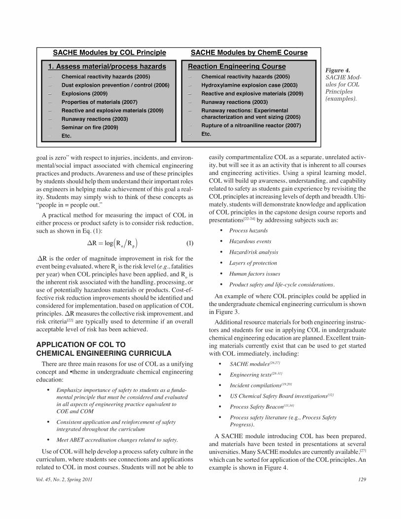
Vol. 45, No. 2, Spring 2011 129
goal is zero” with respect to injuries, incidents, and environ-mental/social impact associated with chemical engineering practices and products. Awareness and use of these principles by students should help them understand their important roles as engineers in helping make achievement of this goal a real-ity. Students may simply wish to think of these concepts as “people in = people out.”
A practical method for measuring the impact of COL in either process or product safety is to consider risk reduction, such as shown in Eq. (1):
∆ = ( )R R Ro plog ( )1
∆R is the order of magnitude improvement in risk for the event being evaluated, where Rp is the risk level (e.g., fatalities per year) when COL principles have been applied, and Ro is the inherent risk associated with the handling, processing, or use of potentially hazardous materials or products. Cost-ef-fective risk reduction improvements should be identified and considered for implementation, based on application of COL principles. ∆R measures the collective risk improvement, and risk criteria[22] are typically used to determine if an overall acceptable level of risk has been achieved.
APPLICATION OF COL TOCHEMICAL ENGINEERING CURRICULA
There are three main reasons for use of COL as a unifying concept and •theme in undergraduate chemical engineering education:
• Emphasize importance of safety to students as a funda-mental principle that must be considered and evaluated in all aspects of engineering practice equivalent to COE and COM
• Consistent application and reinforcement of safety integrated throughout the curriculum
• Meet ABET accreditation changes related to safety.
Use of COL will help develop a process safety culture in the curriculum, where students see connections and applications related to COL in most courses. Students will not be able to
easily compartmentalize COL as a separate, unrelated activ-ity, but will see it as an activity that is inherent to all courses and engineering activities. Using a spiral learning model, COL will build up awareness, understanding, and capability related to safety as students gain experience by revisiting the COL principles at increasing levels of depth and breadth. Ulti-mately, students will demonstrate knowledge and application of COL principles in the capstone design course reports and presentations[22-24] by addressing subjects such as:
• Process hazards
• Hazardous events
• Hazard/risk analysis
• Layers of protection
• Human factors issues
• Product safety and life-cycle considerations.
An example of where COL principles could be applied in the undergraduate chemical engineering curriculum is shown in Figure 3.
Additional resource materials for both engineering instruc-tors and students for use in applying COL in undergraduate chemical engineering education are planned. Excellent train-ing materials currently exist that can be used to get started with COL immediately, including:
• SACHE modules[26,27]
• Engineering texts[28-31]
• Incident compilations[19,20]
• US Chemical Safety Board investigations[32]
• Process Safety Beacon[33,34]
• Process safety literature (e.g., Process Safety Progress).
A SACHE module introducing COL has been prepared, and materials have been tested in presentations at several universities. Many SACHE modules are currently available,[27] which can be sorted for application of the COL principles. An example is shown in Figure 4.
1. Assess material/process hazards1. Assess material/process hazards–– Chemical reactivity hazards (2005)Chemical reactivity hazards (2005)–– Dust explosion prevention / control (2006)Dust explosion prevention / control (2006)–– Explosions (2009)Explosions (2009)–– Properties of materials (2007)Properties of materials (2007)–– Reactive and explosive materials (2009)Reactive and explosive materials (2009)–– Runaway reactions (2003)Runaway reactions (2003)–– Seminar on fire (2009)Seminar on fire (2009)–– Etc.Etc.
Reaction Engineering CourseReaction Engineering Course–– Chemical reactivity hazards (2005)Chemical reactivity hazards (2005)–– Hydroxylamine explosion case (2003)Hydroxylamine explosion case (2003)–– Reactive and explosive materials (2009)Reactive and explosive materials (2009)–– Runaway reactions (2003)Runaway reactions (2003)–– Runaway reactions: Experimental Runaway reactions: Experimental
characterization and vent sizing (2005)characterization and vent sizing (2005)–– Rupture of a Rupture of a nitroanilinenitroaniline reactor (2007)reactor (2007)–– Etc.Etc.
SACHE Modules by COL Principle SACHE Modules by ChemE Course
Figure 4. SACHE Mod-ules for COL Principles (examples).
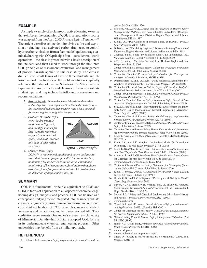
Chemical Engineering Education130
EXAMPLEA simple example of a classroom active-learning exercise
that reinforces the principles of COL in a separations course was adapted from the April 2003 Process Safety Beacon.[33,34] The article describes an incident involving a fire and explo-sion originating in an activated carbon drum used to control hydrocarbon emissions from a flammable liquids storage ter-minal. Starting with COL principle four—consider real-world operations—the class is presented with a basic description of the incident, and then asked to work through the first three COL principles of assessment, evaluation, and management of process hazards applied to this case study. The class is divided into small teams of two or three students and al-lowed a short time to work on the problem. Students typically reference the table of Failure Scenarios for Mass Transfer Equipment.[7] An instructor-led classroom discussion solicits student input and may include the following observations and recommendations:
1. Assess Hazards: Flammable materials exist in the carbon bed and hydrocarbon vapor, and low thermal conductivity in the carbon bed reduces heat transfer rates with a potential for exceeding the auto-ignition temperature.
2. Evaluate Hazards: Refer-ence the fire triangle, as shown in Figure 5, and identify sources for fuel (organic materials), oxygen (air in the tank space) and heat (exother-mic heat of adsorption reaction).
3. Manage Risk: Apply LOPA[10] to recommend passive and active design solu-tions that include: proper flow distribution in the bed, minimizing the bed cross sectional area, continuous monitoring of bed temperature, flooding/inerting, flame arresters, foam fire protection, interlock to isolate feed on detection of high temperature, etc.
SUMMARYCOL is a fundamental principle equivalent to COE and
COM in terms of application to all aspects of chemical engi-neering design, analysis, and practice. COL can be used as a concept and unifying theme integrated into the undergraduate chemical engineering curriculum to emphasize and reinforce consistent application of COL principles, increase student awareness and capabilities, and help meet revised ABET ac-creditation requirements. One author’s university—University of Minnesota, Duluth—has officially adopted COL for use in its undergraduate chemical engineering program. Other universities may benefit from a similar approach.
REFERENCES 1. DeBlois, L.A., Industrial Safety Organization for Executive and En-
gineer, McGraw Hill (1926) 2. Petersen, P.B., Lewis A. DeBlois and the Inception of Modern Safety
Management at DuPont, 1907-1926, submitted to Academy ofManage-ment, Management History, Division, Hagley Museum and Library, Wilmington, DE, ca 1987
3. Klein, J.A., “Two Centuries of Process Safety at DuPont,” Process Safety Progress, 28(24) (2009)
4. DeBlois, L.A., “The Safety Engineer,” American Society of Mechanical Engineers, Hagley Museum and Library, Wilmington, DE (1918)
5. Chemical Safety Board, Investigation Report, T2 Laboratories, Inc., Runaway Reaction, Report No. 2008-3-I-FL, Sept. 2009
6. AICHE, Letter to Mr. John Bresland from H. Scott Fogler and June Wispelwey, Dec. 7, 2009
7. Center for Chemical Process Safety, Guidelines for Hazard Evaluation Procedures, 3rd Ed., John Wiley & Sons (2008)
8. Center for Chemical Process Safety, Guidelines for Consequence Analysis of Chemical Releases, AICHE (1999)
9. Dharmavaram, S., and J.A. Klein, “Using Hazards Assessment to Pre-vent Loss of Containment,” Process Safety Progress, 29(4) (2010)
10. Center for Chemical Process Safety, Layer of Protection Analysis: Simplified Process Risk Assessment, John Wiley & Sons (2001)
11. Center for Chemical Process Safety, Guidelines for Chemical Process Quantitative Risk Analysis, AICHE (1999)
12. Center for Chemical Process Safety, Inherently Safer Chemical Pro-cesses: A Life Cycle Approach, 2nd Ed., John Wiley & Sons (2008)
13. Seay, J.R., and M.R. Eden, “Incorporating Risk Assessment and Inher-ently Safer Design Practices into Chemical Engineering Education,” Chem. Eng. Ed., 42(3) (2008)
14. Center for Chemical Process Safety, Guidelines for Implementing Process Safety Management Systems, AICHE (1993)
15. Center for Chemical Process Safety, Guidelines for Risk Based Process Safety, John Wiley & Sons (2007)
16. Center for Chemical Process Safety, Human Factors Methods for Improv-ing Performance in the Process Industries, John Wiley & Sons (2007)
17. Kletz, T., An Engineer’s View of Human Error, 3rd Ed., IChemE, Rugby, UK (2001)
18. Klein, J.A., and B.K. Vaughen, “A Revised Model for Operational Discipline,” Process Safety Progress, 27(1) (2008)
19. Kletz, T., What Went Wrong? Case Histories of Process Plant Disasters and How They Could Have Been Avoided, 5th Ed., Elsevier (2009)
20. Atherton, J., and F. Gil, Incidents That Define Process Safety, Center for Chemical Process Safety, John Wiley & Sons (2008)
21. <www2.dupont.com/sustainability/en_US/> 22. Center for Chemical Process Safety, Guidelines for Developing Quan-
titative Safety Risk Criteria, John Wiley & Sons (2009) 23. Kletz, T., Process Plants: A Handbook for Inherently Safer Design,
Taylor & Francis, Philadelphia (1998) 24. Ulrich, G.D., and T.V. Palligarnai, “Predesign with Safety in Mind,”
Chem. Eng. Progress, July, 2006 25. Turton, R., R.C. Bailie, W.B. Whiting, and J.A. Shaeiwitz, Analysis,
Synthesis, and Design of Chemical Processes, 3rd Ed., Prentice Hall, Upper Saddle River, NJ (2009)
26. Louvar, J.F., “Safety and Chemical Engineering Education—History and Results,” Process Safety Progress, 28(2) (2009)
27. <www.sache.org> 28. Crowl, D.A., and J.F. Louvar, Chemical Process Safety: Fundamentals
and Applications, 2nd Ed., Prentice Hall (2001) 29. Center for Chemical Process Safety, Guidelines for Design Solutions
for Process Equipment Failures, AIChE (1998) 30. National Safety Council, Product Safety Management Guidelines, 2nd
Ed., NSC (1997) 31. Horne, R., T. Grant, and K. Verghese, Life Cycle Assessment: Principles,
Practice, and Prospects, CSIRO (2009) 32. <www.csb.gov> 33. <www.sache.org/beacon/products.asp> 34. Luper, D., “Create Effective Process Safety Moments,” Chem. Eng.
Progress (2010) p
HEAT
FUEL OXYGEN
Figure 5. Fire triangle.
Vol. 45, No. 2, Spring 2011 131
Richard M. Felder is Hoechst Celanese Professor Emeritus of Chemical Engineering at North Carolina State University. He is co-author of Elementary Principles of Chemical Processes (Wiley, 2005) and numerous articles on chemical process engineering and engineering and science education, and regularly presents workshops on ef-fective college teaching at campuses and conferences around the world. Many of his publications can be seen at <www.ncsu.edu/effective_teaching>.
Random Thoughts . . .
Dear Dr. Felder,
What can I do about low teaching evaluations from students I teach actively when what they clearly want is much more traditional (passive ride, smooth highway please)? I’m about ready to give up and return to just lecturing, as I am sure students will evaluate my courses higher if I do. Thank you for your time and consideration.
Sincerely, _____________
* * *Dear ____________,
Before I respond to your question, let me assure you that I get it. Learner-centered teaching methods like active and cooperative and problem-based learning make students take more responsibility for their learning than traditional teacher-centered methods do, and the students are not necessarily thrilled about it. All college instructors who have tried the former methods have experienced student resistance—and if they were getting high evaluations when they taught tradi-tionally, their ratings may have dropped when they made the switch. As you’ve discovered, it doesn’t feel good when that happens, so it will be understandable if you decide to go back to teaching classes where you just lecture and the students just listen (or text or surf or daydream or sleep).
Please think about a couple of things before you make your decision, however. An important part of our job as teachers is equipping as many of our students as possible with high-level problem-solving and thinking skills, including critical and creative thinking. If there’s broad agreement about anything in educational research, it’s that well-implemented learner-centered instruction is much more effective than traditional lecture-based instruction at promoting those skills. (If you’d
HANG IN THERE!Dealing with Student Resistance
to Learner-Centered Teaching
riChard m. FEldEr
like to check the research for yourself, the attached bibli-ography suggests some good starting points.) It’s true that many students want us to simply tell them up front in our lectures everything they need to know for the exam rather than challenging them to figure any of it out for themselves. If we give them that, though, we are failing those who have an aptitude for high-level thinking and problem solving but might not develop those skills without the guidance, practice, and feedback learner-centered methods provide. That failure is a high price for us to pay to get better student ratings—and we might not even get them by staying traditional. Teachers whose evaluations are not all that high to begin with com-monly see their ratings increase when they adopt a more learner-centered approach.
I don’t know what your institution is like, but here’s the way things go at the universities and colleges I’ve visited. Most instructors teach traditionally but there are quite a few who use active learning and other learner-centered methods, including some of the best teachers on the campus—the ones who routinely get excellent performance and high ratings from their students, teaching awards, and wedding invitations and birth announcements from their former students. At some point another faculty member may decide to try, say, active
© Copyright ChE Division of ASEE 2011
Chemical Engineering Education132
All of the Random Thoughts columns are now available on the World Wide Web athttp://www.ncsu.edu/effective_teaching and at http://che.ufl.edu/~cee/
learning, perhaps after attending a workshop or reading a paper or constantly hearing about the superb student responses their gifted colleague always enjoys. He or she tries it and it doesn’t go well—the evaluations are mediocre and some students grumble that their professor made them do all the work instead of teaching them.* Instructors in this situation can easily conclude that the nontraditional methods caused their poor ratings. What that conclusion doesn’t explain, however, is how that talented colleague of theirs can use the same methods on the same students and get good performance and glowing reviews.
Whenever I’ve explored this issue with instructors dis-tressed by it, I have invariably found that the teaching method they were trying was not the real problem. It was either that they were making one or more mistakes in implementing the method, or something else was troubling the students and the method was a convenient scapegoat. So, if you’ve used a learner-centered method, didn’t like the outcomes, and would like to do some exploring, you might start with these questions:
• In your student evaluations, were complaints limited to the method, or did they also relate to other things such as the length of your assignments and exams, the clarity of your lecturing, or your lack of availability and/or respect for students? If they did, consider addressing those complaints before abandoning the method.
• Did you explain to the students why you were using the method? If you tell them you’re doing it because research has shown that it leads to improved learning, greater acquisition of skills that potential employers consider valuable, and higher grades, most will set aside their objections long enough to find that you’re telling the truth. (See Reference 2 in the bibliography.)
• Did you use the new method long enough to overcome the learning curve associated with it? It can take most of a semester to become comfortable with and adept at active learning, and if you’re using a more com-plex technique such as cooperative or problem-based learning and you’re not being mentored by an expert, it might take several years.
• If you got unsatisfactory student ratings, did you check references on the method to see if you were doing something wrong? For example, did you assign small-group activities in class that lasted for more than 2–3 minutes or call for volunteers to respond every time? (See Reference 4 to find out how both practices can kill the effectiveness of active learning.) The bibliography suggests references you might consult for each of the most common learner-centered methods.
• In your midterm evaluations, did you specifically ask the students whether they thought active learning (or whatever you were doing) was (a) helping their learn-ing, (b) hindering their learning, or (c) neither helping nor hindering? If you do this, you may find that the students objecting vigorously to the method are only a small minority of the class. If that’s so, announce the survey results in the next class session. Students who complain about learner-centered methods often imagine that they are speaking for most of their class-mates. Once they find out that very few others feel the way they do, the grumbling tends to disappear immediately.
If your answers to any of those questions suggest that making some changes in your approach to the method and trying again might be worthwhile, consider doing it. If you conclude, however, that you’ve done all you can and going back to traditional teaching is your only viable course of ac-tion, then so be it. I hope you choose the first option, but it’s totally your call.
Best regards, and good luck, Richard Felder
BIBLIOGRAPHY 1. Bullard L.G., and R.M. Felder, “A Learner-centered Approach to Teach-
ing Material and Energy Balances. 1. Course Design,” Chem. Eng. Ed., 41(2), 93 <http://www.ncsu.edu/felder-public/Papers/StoichPap-pt1.pdf>; “2. Course Instruction and Assessment,” Chem. Eng. Ed., 41(3), 167 <http://www.ncsu.edu/felder-public/Papers/StoichPap-pt2.pdf> (2007)
2. Felder, R.M., Sermons for Grumpy Campers,” Chem. Eng. Ed., 41(3), 183, <http://www.ncsu.edu/felder-public/Columns/Sermons.pdf> (2007)
3. Felder, R.M., and R. Brent, “Cooperative Learning,” in P.A. Mabrouk, ed., Active Learning: Models from the Analytical Sciences, ACS Symposium Series 970, Chapter 4, 34–53, Washington, DC: American Chemical Society, <http://www.ncsu.edu/felder-public/Papers/CL-Chapter.pdf> (2007)
4. Felder, R.M., and R. Brent, “Active Learning: An Introduction,” ASQ Higher Education Brief, 2(4), <http://www.ncsu.edu/felder-public/Pa-pers/ALpaper(ASQ).pdf> (2009)
5. Prince, M.J., “Does Active Learning Work? A Review of the Research,” J. Eng. Ed., 93(3), 223, <http://www.ncsu.edu/felder-public/Papers/Prince_AL.pdf> (2004)
6. Prince, M.J., and R.M. Felder, “Inductive Teaching and Learning Meth-ods: Definitions, Comparisons, and Research Bases,” J. Eng. Ed., 95(2), 123, <http://www.ncsu.edu/felder-public/Papers/InductiveTeaching.pdf> (Inductive methods include inquiry-based, problem-based, and project-based learning.) (2006) p
* My favorite student evaluation came from someone who wrote “Felder really makes us think!” It was on his list of the three things he disliked most about the course.
Vol. 45, No. 2, Spring 2011 133
One educational goal of the unit operations laboratory is to help students understand fundamental principles by connecting theory and equations in their textbooks
to real-world applications. We have found, however, that collecting data and analyzing it with empirical correlations does not always translate into a good understanding of what is happening inside the pipes.[1] One problem is that the theoretical development behind the labs is often comprised of approximate methods using lumped parameters that de-scribe the results but not the details of the physical process. For example, when a mass transfer coefficient is obtained from an absorption experiment, some students struggle to explain what the mass transfer coefficient represents and why it increases with increasing absorbent flow rate. To address this problem, we are using computer simulations to solidify the link between experiment and theory and provide improved learning.[1,2]
Commercial software packages like COMSOL Multiphys-icsTM allow students to set up and solve the partial differential equations that describe momentum, energy, and mass balances and also to visualize the velocity, pressure, temperature, and concentration profiles within the equipment. Visualization of the processes may not only help reinforce concepts and clarify the underlying physics but it may also help “bring to life” the mathematics as well as the experiments. With this software, students don’t necessarily need to know the details of how to solve complex equations, but they need to know
which equations to solve and how to validate the results.[3] This type of simulation can also extend the range of experi-ence beyond what is possible in the lab by allowing studies that would otherwise be prohibited by time, financial, or safety constraints.
In this paper we present experiments and computer mod-els for studying the environmentally important problem of removing CO2 from air. Simple models are shown to provide straightforward analysis of the experimental data even when the system is not dilute. In addition, we present more detailed models that illustrate the two-film theory and provide insight
William Clark is an associate professor of chemical engineering at Worcester Polytechnic Institute. He received a B.S. degree from Clemson University and a Ph.D. degree from Rice University, both in chemical engineering. He has more than 20 years of experience teaching thermo-dynamics and unit operations laboratory at WPI. In addition to research efforts in teaching and learning, he has conducted disciplinary research in separation processes.
Yaminah Jackson graduated from the WPI Chemical Engineering De-partment in Spring 2008. She is currently attending graduate school at the University of Southern California.
Michael Morin graduated from the WPI Chemical Engineering Depart-ment in Spring 2009. He is currently a Ph.D. candidate in mechanical engineering at WPI.
Giacomo Ferraro is the laboratory manager in the Chemical Engineering Department at WPI. He is a master machinist and has facilitated equip-ment design, fabrication, and use for teaching and research at WPI for more than 30 years.
Combining Experiments and Simulation of Gas Absorption for Teaching Mass Transfer Fundamentals:
REMOVING CO2 FROM AIRUSING WATER AND NAOH
William m. ClarK, yaminah z. JaCKSon, miChaEl t. morin, and giaComo p. FErraro
Worcester Polytechnic Institute, Worcester MA 01609
© Copyright ChE Division of ASEE 2011
ChE laboratory
Chemical Engineering Education134
into the absorption process. These models help explain the absorbent flow rate dependence of the mass transfer coeffi-cient and how the process is liquid phase resistance controlled when using water and dependent on the gas phase resistance when using dilute NaOH solution as absorbent. Finally, we provide some discussion of how the simulations have been received by students.
LABORATORY EXPERIMENTA few years ago our old 30-foot-tall, 6-inch-diameter, steel
absorption tower became clogged with rust and residue from years of use with sodium carbonate solution as absorbent for removing CO2 from air. Since concerns over global warming are a political reality even if the causes and effects are not clear, we wanted to continue to offer a CO2 absorption experi-ment because of its appeal to student interest as well as its ability to illustrate mass transfer fundamentals. To reduce cost and avoid column fouling in the future, we chose to use pure water as absorbent in our new 6-foot-tall, 3-inch-diameter, glass column packed with 54 inches of ¼-inch glass Raschig rings that we purchased from Hampden Engineering Corpora-tion[4] and modified to suit our needs. Although using water as absorbent focuses the lab on mass transfer concepts without the added complexity of reactions, the limited solubility of CO2 in water makes it necessary to have accurate analysis of the gas phase and to work with concentrated gas streams to get good results. A Rosemount Analytical, Inc.,[5] model 880a infrared analyzer provides accurate and reliable measure-ment of the CO2 composition of the gas phase at the column entrance and exit. To measure a significant change in the gas phase composition, it is best if the gas rate is low and the water rate is high. Having a low gas rate also provides the benefit of consuming less CO2 (and air) and emitting less CO2 to the environment in both the exiting gas and water streams.
To illustrate the advantage of combining a chemical reaction with the absorption process, we also built a small-scale column for use with NaOH solution as absorbent. A 1.75-in-diameter, 15-in-long acrylic tube was filled to a height of 12.75 in with the same glass rings used in our larger column.
End caps for the acrylic column were made with rubber stop-pers fitted with liquid and gas inlet and outlets.
We describe here the analysis of representative sets of ex-perimental runs using the two columns. Our students use the larger column to determine the effect of water flow rate on the mass transfer process. Experimental data are presented in Table 1 for four different water flow rates at fixed gas phase inlet conditions and room temperature. At present we don’t have our students working with NaOH in the lab for safety reasons. Instead, we give them data obtained on the smaller column by a student working on his senior thesis. Table 2 shows the data collected for both water and 1 N NaOH solu-tion at five different liquid rates and a fixed gas phase inlet condition at room temperature. It can be seen that very little CO2 is removed in the small column at these conditions with water as absorbent. On the other hand, most of the CO2 is removed from the gas stream when NaOH is used, even in the small column.
TABLE 1Large Column Data and Results for CO2 Absorption
from Air Using Water at Room TemperatureAir Rate, A = 1.42 L/min; Inlet CO2, yb = 0.185
Water Rate, W L/min
Outlet CO2, ytmole fraction
Kyamol/m3s
0.53 0.143 0.333
1.06 0.099 0.558
1.58 0.064 0.634
2.11 0.039 0.712
TABLE 2Small Column Data and Results for CO2 Absorption From Air Using Water
or 1 N NaOH at Room Temperature
Air Rate, A = 1.5 L/minyb = 0.175 (water) yb = 0.178 (NaOH)
Liquid Rate, WL/min
Outlet CO2 , ytmole fraction
Kyamol/m3s
Outlet CO2, ytmole fraction
Kyamol/m3s
0.14 0.168 0.237 0.062 2.96
0.23 0.165 0.285 0.050 3.69
0.28 0.164 0.312 0.037 4.09
0.35 0.162 0.349 0.031 4.66
0.40 0.161 0.375 0.027 5.07
TABLE 3Heights of Transfer Units and Mass Transfer Coefficients for Large Column
Water Rate L/min
Hxm
Hym
mGHx/L m
HOym
kya mol/m3s
kxa mol/m3s
kxa/mmol/m3s
Kya correlated
0.53 0.193 0.065 0.591 0.656 3.55 557 0.392 0.353
1.06 0.238 0.046 0.363 0.410 5.02 904 0.637 0.565
1.58 0.268 0.038 0.275 0.313 6.13 1196 0.842 0.740
2.11 0.292 0.033 0.225 0.257 7.08 1464 1.031 0.900
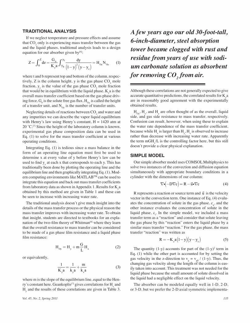
Vol. 45, No. 2, Spring 2011 135
TRADITIONAL ANALYSISIf we neglect temperature and pressure effects and assume
that CO2 only is experiencing mass transfer between the gas and the liquid phases, traditional analysis leads to a design equation for our absorber given by[6]:
Z dzGK a
dy
y y yH N
Z
y e
Oy Oyy
y
b
t= =
−( ) −( )=∫ ∫0
02
11( )
where t and b represent top and bottom of the column, respec-tively, Z is the column height, y is the gas phase CO2 mole fraction, ye is the value of the gas phase CO2 mole fraction that would be in equilibrium with the liquid phase, Kya is the overall mass transfer coefficient based on the gas phase driv-ing force, G0 is the solute free gas flux, HOy is called the height of a transfer unit, and NOy is the number of transfer units.
Neglecting details of reactions between CO2 and water and any impurities we can describe the vapor liquid equilibrium with Henry’s law using Henry’s constant, H = 1420 atm at 20 ˚C.[7] Since the height of the laboratory column is known, experimental gas phase composition data can be used in Eq. (1) to solve for the mass transfer coefficient at various operating conditions.
Integrating Eq. (1) is tedious since a mass balance in the form of an operating line equation must first be used to determine x at every value of y before Henry’s law can be used to find ye at each x that corresponds to each y. This has traditionally been done by plotting the operating line and the equilibrium line and then graphically integrating Eq. (1). Mod-ern computing environments like MATLABTM can be used to integrate this equation and back out mass transfer coefficients from laboratory data as shown in Appendix 1. Results for Kya obtained by this method are given in Table 1 and these can be seen to increase with increasing water rate.
The traditional analysis doesn’t give much insight into the details of the mass transfer process or the physical reason the mass transfer improves with increasing water rate. To obtain that insight, students are directed to textbooks for an expla-nation of the two-film theory of Whitman[8] where they learn that the overall resistance to mass transfer can be considered to be made of a gas phase film resistance and a liquid phase film resistance:
H H mGLHOy y x= + ( )2
or equivalently,
1 1 3K a k a
mk ay y x
= + ( )
where m is the slope of the equilibrium line, equal to the Hen-ry’s constant here. Geankoplis[7] gives correlations for Hx and Hy and the results of these correlations are given in Table 3.
Although these correlations are not generally expected to give accurate quantitative predictions, the correlated results for Kya are in reasonably good agreement with the experimentally obtained results.
HOy, Hx, and Hy are often thought of as the overall, liquid side, and gas side resistance to mass transfer, respectively. Confusion can result, however, when using these to explain the water rate dependence of the mass transfer coefficient, because while Hx is larger than Hy, Hx is observed to increase rather than decrease with increasing water rate. Apparently the term mGHx/L is the controlling factor here, but this still doesn’t provide a clear physical explanation.
SIMPLE MODELOur simple absorber model uses COMSOL Multiphysics to
solve two instances of the convection and diffusion equation simultaneously with appropriate boundary conditions in a cylinder with the dimensions of our column:
∇ − ∇( )= − ∇i�iD c R u c ( )4
R represents a reaction or source term and �u is the velocity vector in the convection term. One instance of Eq. (4) evalu-ates the concentration of solute in the gas phase, cg, and the other instance evaluates the concentration of solute in the liquid phase, cl. In the simple model, we included a mass transfer term as a “reaction” and consider that solute leaving the gas phase by this “reaction” enters the liquid phase by a similar mass transfer “reaction.” For the gas phase, the mass transfer “reaction” was written as
R K a y y yy e=− −( ) −( )1 5( )
The quantity (1-y) accounts for part of the (1-y)2 term in Eq. (1) while the other part is accounted for by setting the gas velocity in the z-direction to vg = vg0 / (1-y). Thus, the changing gas velocity along the length of the column is eas-ily taken into account. This treatment was not needed for the liquid phase because the small amount of solute dissolved in the liquid had a negligible effect on the liquid velocity.
The absorber can be modeled equally well in 1-D, 2-D, or 3-D, but we prefer the 2-D axial symmetric implementa-
A few years ago our old 30-foot-tall, 6-inch-diameter, steel absorption tower became clogged with rust and residue from years of use with sodi-um carbonate solution as absorbent for removing CO2 from air.
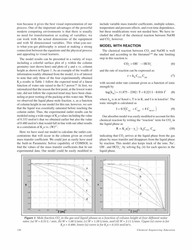
Chemical Engineering Education136
tion because it gives the best visual representation of our process. One of the important advantages of the powerful modern computing environments is that there is usually no need for transformation or scaling of variables; we can work with the actual dimensions of the equipment and with SI dimensioned variables. This what-you-see-is-what-you-get philosophy is aimed at making a strong connection between the equations and the physical process and appealing to visual learners.
The model results can be presented in a variety of ways including a colorful surface plot of y within the column geometry (not shown here) and plots of y and x vs. column height as shown in Figure 1. As an example of the wealth of information readily obtained from the model, it is of interest to note that only three of the four experimentally obtained Kya results in Table 1 follow the expected trend of a linear function of water rate raised to the 0.7 power.[6] At first, we rationalized that the reason the first point, at the lowest water rate, did not follow the expected trend may have been chan-neling or poor wetting of the packing at this water rate. When we observed the liquid phase mole fraction, x, as a function of column height in our model for this run, however, we saw that the liquid was essentially saturated before reaching the column outlet. Thus, the experimental outlet results can be modeled using a wide range of Kya values including the value of 0.333 mol/m3s that we obtained earlier but also the value of 0.480 mol/m3s that would fall in line with our other results in a correlation of Kya vs. (W)0.7.
Here we have used our model to calculate the outlet con-centrations that will occur in the column given an overall mass transfer coefficient. We could just as easily have used the built-in Parametric Solver capability of COMSOL to find the values of the mass transfer coefficients that fit our experimental data. Our model could be easily modified to
include variable mass transfer coefficients, multiple solutes, temperature and pressure effects, and even time dependence, but these modifications were not needed here. We have in-cluded the effect of the chemical reaction between NaOH and CO2, however.
MODEL WITH REACTIONThe chemical reaction between CO2 and NaOH is well
studied and according to the literature[10] the rate limiting step in this reaction is:
CO OH HCO2 3 6+ →− − ( )
and the rate of reaction can be expressed as:
r k C CB CO OH= −2 7( )
with second order rate constant given as a function of ionic strength by
log . / . . ( )k T I IB( )= − + −11 875 2382 0 221 0 016 82
where kB is in m3/kmol s, T is in K, and I is in kmol/m3. The ionic strength is calculated as
I C C CNa OH HCO
= + +( )+ − −0 5 4 93
. ( )
Our absorber model was easily modified to account for this chemical reaction by writing the “reaction” term for CO2 in the liquid phase as
R K a y y k C Cy e B CO OH= −( )− −2 10( )
indicating that CO2 arrives at the liquid phase from the gas phase by mass transfer and disappears from the liquid phase by reaction. This model also keeps track of the ions, Na+, OH–, and HCO3
–, by solving Eq. (4) for each species in the liquid phase.
Figure 1. Mole fraction CO2 in the gas and liquid phases as a function of column height at four different water rates: (a) W = 0.53 L / min, (b) W = 1.06 L/min, (c) W = 1.58 L/min, and (d) W = 2.11 L/min. Upper (a) curve is for
Kya = 0.480, lower (a) curve is for Kya = 0.333 mol/m3s.
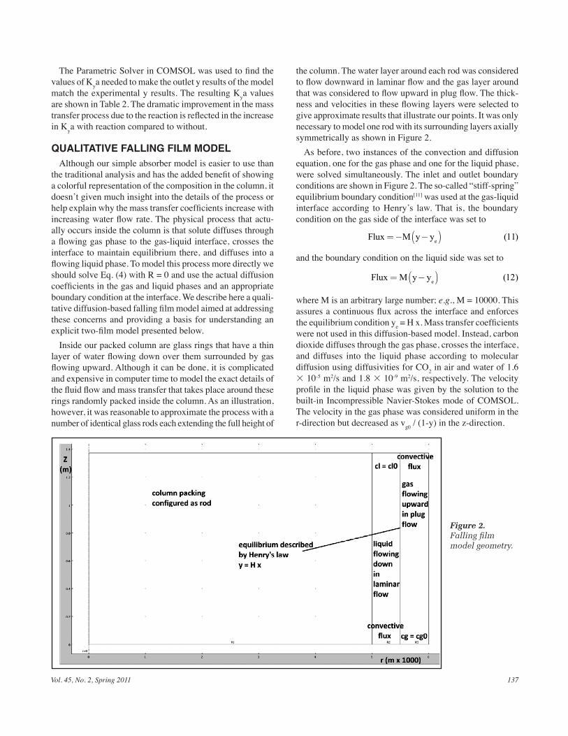
Vol. 45, No. 2, Spring 2011 137
The Parametric Solver in COMSOL was used to find the values of Kya needed to make the outlet y results of the model match the experimental y results. The resulting Kya values are shown in Table 2. The dramatic improvement in the mass transfer process due to the reaction is reflected in the increase in Kya with reaction compared to without.
QUALITATIVE FALLING FILM MODELAlthough our simple absorber model is easier to use than
the traditional analysis and has the added benefit of showing a colorful representation of the composition in the column, it doesn’t given much insight into the details of the process or help explain why the mass transfer coefficients increase with increasing water flow rate. The physical process that actu-ally occurs inside the column is that solute diffuses through a flowing gas phase to the gas-liquid interface, crosses the interface to maintain equilibrium there, and diffuses into a flowing liquid phase. To model this process more directly we should solve Eq. (4) with R = 0 and use the actual diffusion coefficients in the gas and liquid phases and an appropriate boundary condition at the interface. We describe here a quali-tative diffusion-based falling film model aimed at addressing these concerns and providing a basis for understanding an explicit two-film model presented below.
Inside our packed column are glass rings that have a thin layer of water flowing down over them surrounded by gas flowing upward. Although it can be done, it is complicated and expensive in computer time to model the exact details of the fluid flow and mass transfer that takes place around these rings randomly packed inside the column. As an illustration, however, it was reasonable to approximate the process with a number of identical glass rods each extending the full height of
the column. The water layer around each rod was considered to flow downward in laminar flow and the gas layer around that was considered to flow upward in plug flow. The thick-ness and velocities in these flowing layers were selected to give approximate results that illustrate our points. It was only necessary to model one rod with its surrounding layers axially symmetrically as shown in Figure 2.
As before, two instances of the convection and diffusion equation, one for the gas phase and one for the liquid phase, were solved simultaneously. The inlet and outlet boundary conditions are shown in Figure 2. The so-called “stiff-spring” equilibrium boundary condition[11] was used at the gas-liquid interface according to Henry’s law. That is, the boundary condition on the gas side of the interface was set to
Flux M y ye=− −( ) ( )11
and the boundary condition on the liquid side was set to
Flux M y ye= −( ) ( )12
where M is an arbitrary large number; e.g., M = 10000. This assures a continuous flux across the interface and enforces the equilibrium condition ye = H x. Mass transfer coefficients were not used in this diffusion-based model. Instead, carbon dioxide diffuses through the gas phase, crosses the interface, and diffuses into the liquid phase according to molecular diffusion using diffusivities for CO2 in air and water of 1.6 3 10-5 m2/s and 1.8 3 10-9 m2/s, respectively. The velocity profile in the liquid phase was given by the solution to the built-in Incompressible Navier-Stokes mode of COMSOL. The velocity in the gas phase was considered uniform in the r-direction but decreased as vg0 / (1-y) in the z-direction.
Figure 2. Falling film model geometry.
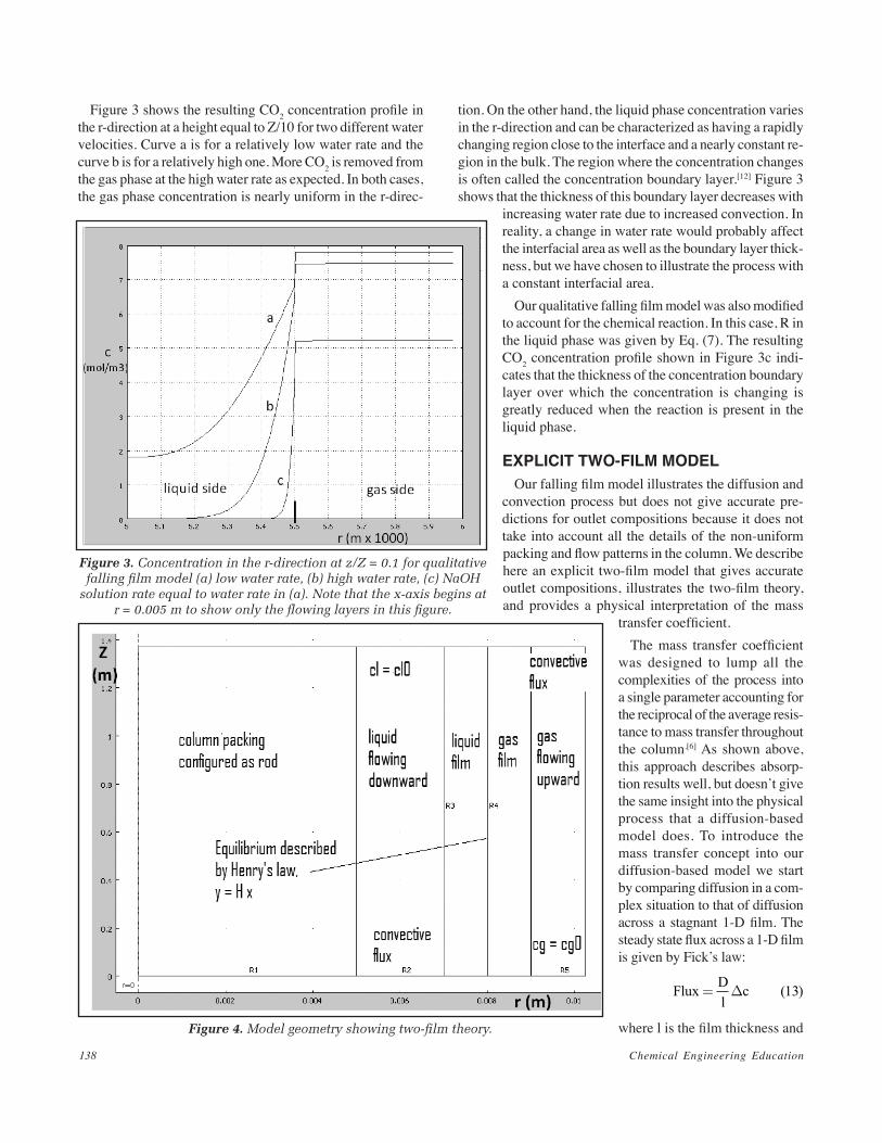
Chemical Engineering Education138
Figure 3 shows the resulting CO2 concentration profile in the r-direction at a height equal to Z/10 for two different water velocities. Curve a is for a relatively low water rate and the curve b is for a relatively high one. More CO2 is removed from the gas phase at the high water rate as expected. In both cases, the gas phase concentration is nearly uniform in the r-direc-
tion. On the other hand, the liquid phase concentration varies in the r-direction and can be characterized as having a rapidly changing region close to the interface and a nearly constant re-gion in the bulk. The region where the concentration changes is often called the concentration boundary layer.[12] Figure 3 shows that the thickness of this boundary layer decreases with
increasing water rate due to increased convection. In reality, a change in water rate would probably affect the interfacial area as well as the boundary layer thick-ness, but we have chosen to illustrate the process with a constant interfacial area.
Our qualitative falling film model was also modified to account for the chemical reaction. In this case, R in the liquid phase was given by Eq. (7). The resulting CO2 concentration profile shown in Figure 3c indi-cates that the thickness of the concentration boundary layer over which the concentration is changing is greatly reduced when the reaction is present in the liquid phase.
EXPLICIT TWO-FILM MODELOur falling film model illustrates the diffusion and
convection process but does not give accurate pre-dictions for outlet compositions because it does not take into account all the details of the non-uniform packing and flow patterns in the column. We describe here an explicit two-film model that gives accurate outlet compositions, illustrates the two-film theory, and provides a physical interpretation of the mass
transfer coefficient.The mass transfer coefficient
was designed to lump all the complexities of the process into a single parameter accounting for the reciprocal of the average resis-tance to mass transfer throughout the column.[6] As shown above, this approach describes absorp-tion results well, but doesn’t give the same insight into the physical process that a diffusion-based model does. To introduce the mass transfer concept into our diffusion-based model we start by comparing diffusion in a com-plex situation to that of diffusion across a stagnant 1-D film. The steady state flux across a 1-D film is given by Fick’s law:
Flux Dl
c= ∆ ( )13
where l is the film thickness and
Figure 3. Concentration in the r-direction at z/Z = 0.1 for qualitative falling film model (a) low water rate, (b) high water rate, (c) NaOH
solution rate equal to water rate in (a). Note that the x-axis begins at r = 0.005 m to show only the flowing layers in this figure.
Figure 4. Model geometry showing two-film theory.
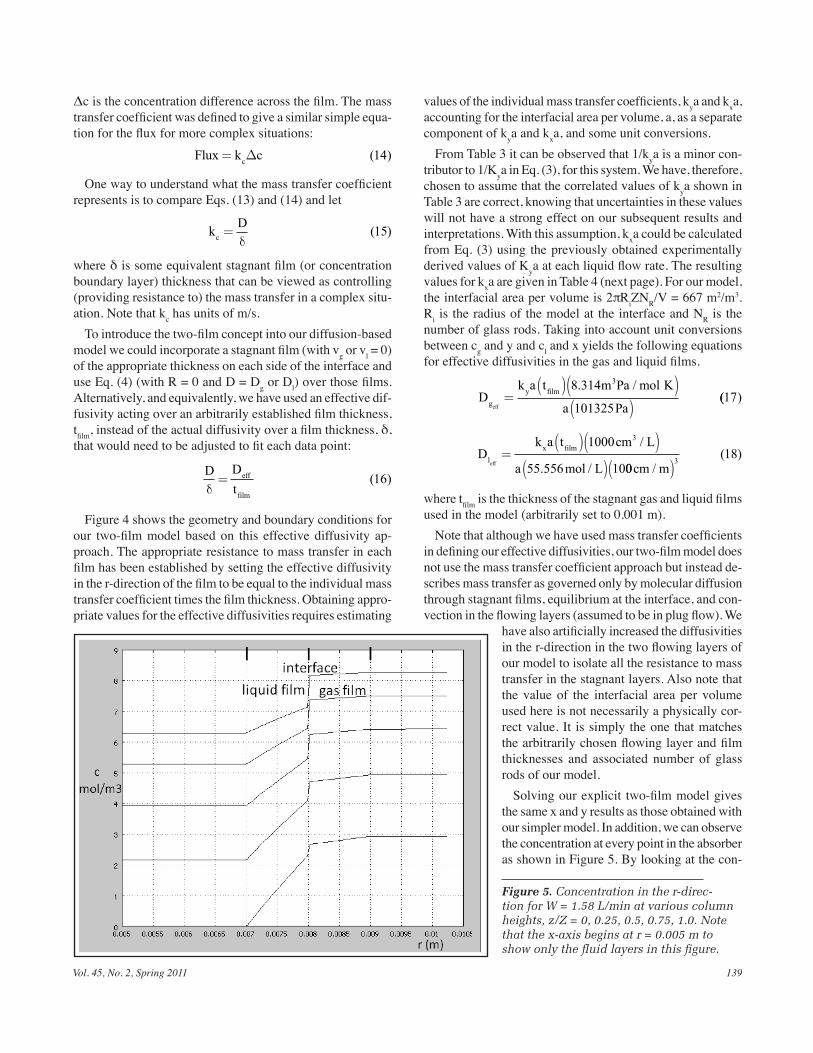
Vol. 45, No. 2, Spring 2011 139
Δc is the concentration difference across the film. The mass transfer coefficient was defined to give a similar simple equa-tion for the flux for more complex situations:
Flux k cc= ∆ ( )14
One way to understand what the mass transfer coefficient represents is to compare Eqs. (13) and (14) and let
k Dc = δ
( )15
where δ is some equivalent stagnant film (or concentration boundary layer) thickness that can be viewed as controlling (providing resistance to) the mass transfer in a complex situ-ation. Note that kc has units of m/s.
To introduce the two-film concept into our diffusion-based model we could incorporate a stagnant film (with vg or vl = 0) of the appropriate thickness on each side of the interface and use Eq. (4) (with R = 0 and D = Dg or Dl) over those films. Alternatively, and equivalently, we have used an effective dif-fusivity acting over an arbitrarily established film thickness, tfilm, instead of the actual diffusivity over a film thickness, δ, that would need to be adjusted to fit each data point:
D Dt
eff
filmδ= ( )16
Figure 4 shows the geometry and boundary conditions for our two-film model based on this effective diffusivity ap-proach. The appropriate resistance to mass transfer in each film has been established by setting the effective diffusivity in the r-direction of the film to be equal to the individual mass transfer coefficient times the film thickness. Obtaining appro-priate values for the effective diffusivities requires estimating
values of the individual mass transfer coefficients, kya and kxa, accounting for the interfacial area per volume, a, as a separate component of kya and kxa, and some unit conversions.
From Table 3 it can be observed that 1/kya is a minor con-tributor to 1/Kya in Eq. (3), for this system. We have, therefore, chosen to assume that the correlated values of kya shown in Table 3 are correct, knowing that uncertainties in these values will not have a strong effect on our subsequent results and interpretations. With this assumption, kxa could be calculated from Eq. (3) using the previously obtained experimentally derived values of Kya at each liquid flow rate. The resulting values for kxa are given in Table 4 (next page). For our model, the interfacial area per volume is 2πRiZNR/V = 667 m2/m3. Ri is the radius of the model at the interface and NR is the number of glass rods. Taking into account unit conversions between cg and y and cl and x yields the following equations for effective diffusivities in the gas and liquid films.
Dk a t m Pa mol K
a Pagy film
eff=
( )( )( )8 314
101325
3. /(( )17
Dk a t cm L
a mol Ll
x film
eff=
( )( )( )
1000
55 556 10
3 /
. / 0018
3cm m/
( )( )
where tfilm is the thickness of the stagnant gas and liquid films used in the model (arbitrarily set to 0.001 m).
Note that although we have used mass transfer coefficients in defining our effective diffusivities, our two-film model does not use the mass transfer coefficient approach but instead de-scribes mass transfer as governed only by molecular diffusion through stagnant films, equilibrium at the interface, and con-vection in the flowing layers (assumed to be in plug flow). We
have also artificially increased the diffusivities in the r-direction in the two flowing layers of our model to isolate all the resistance to mass transfer in the stagnant layers. Also note that the value of the interfacial area per volume used here is not necessarily a physically cor-rect value. It is simply the one that matches the arbitrarily chosen flowing layer and film thicknesses and associated number of glass rods of our model.
Solving our explicit two-film model gives the same x and y results as those obtained with our simpler model. In addition, we can observe the concentration at every point in the absorber as shown in Figure 5. By looking at the con-
Figure 5. Concentration in the r-direc-tion for W = 1.58 L/min at various column heights, z/Z = 0, 0.25, 0.5, 0.75, 1.0. Note that the x-axis begins at r = 0.005 m to show only the fluid layers in this figure.
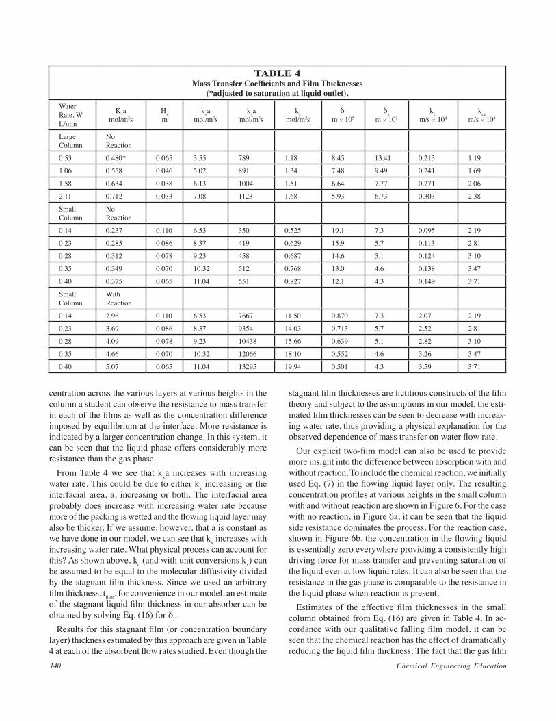
Chemical Engineering Education140
centration across the various layers at various heights in the column a student can observe the resistance to mass transfer in each of the films as well as the concentration difference imposed by equilibrium at the interface. More resistance is indicated by a larger concentration change. In this system, it can be seen that the liquid phase offers considerably more resistance than the gas phase.
From Table 4 we see that kxa increases with increasing water rate. This could be due to either kx increasing or the interfacial area, a, increasing or both. The interfacial area probably does increase with increasing water rate because more of the packing is wetted and the flowing liquid layer may also be thicker. If we assume, however, that a is constant as we have done in our model, we can see that kx increases with increasing water rate. What physical process can account for this? As shown above, kc (and with unit conversions kx) can be assumed to be equal to the molecular diffusivity divided by the stagnant film thickness. Since we used an arbitrary film thickness, tfilm, for convenience in our model, an estimate of the stagnant liquid film thickness in our absorber can be obtained by solving Eq. (16) for δl.
Results for this stagnant film (or concentration boundary layer) thickness estimated by this approach are given in Table 4 at each of the absorbent flow rates studied. Even though the
stagnant film thicknesses are fictitious constructs of the film theory and subject to the assumptions in our model, the esti-mated film thicknesses can be seen to decrease with increas-ing water rate, thus providing a physical explanation for the observed dependence of mass transfer on water flow rate.
Our explicit two-film model can also be used to provide more insight into the difference between absorption with and without reaction. To include the chemical reaction, we initially used Eq. (7) in the flowing liquid layer only. The resulting concentration profiles at various heights in the small column with and without reaction are shown in Figure 6. For the case with no reaction, in Figure 6a, it can be seen that the liquid side resistance dominates the process. For the reaction case, shown in Figure 6b, the concentration in the flowing liquid is essentially zero everywhere providing a consistently high driving force for mass transfer and preventing saturation of the liquid even at low liquid rates. It can also be seen that the resistance in the gas phase is comparable to the resistance in the liquid phase when reaction is present.
Estimates of the effective film thicknesses in the small column obtained from Eq. (16) are given in Table 4. In ac-cordance with our qualitative falling film model, it can be seen that the chemical reaction has the effect of dramatically reducing the liquid film thickness. The fact that the gas film
TABLE 4Mass Transfer Coefficients and Film Thicknesses
(*adjusted to saturation at liquid outlet).WaterRate, W L/min
Kyamol/m3s
Hym
kya mol/m3s
kxa mol/m3s
kx mol/m2s
δlm 3 105
δgm 3 102
kclm/s 3 104
kcgm/s 3 104
Large Column
No Reaction
0.53 0.480* 0.065 3.55 789 1.18 8.45 13.41 0.213 1.19
1.06 0.558 0.046 5.02 891 1.34 7.48 9.49 0.241 1.69
1.58 0.634 0.038 6.13 1004 1.51 6.64 7.77 0.271 2.06
2.11 0.712 0.033 7.08 1123 1.68 5.93 6.73 0.303 2.38
Small Column
NoReaction
0.14 0.237 0.110 6.53 350 0.525 19.1 7.3 0.095 2.19
0.23 0.285 0.086 8.37 419 0.629 15.9 5.7 0.113 2.81
0.28 0.312 0.078 9.23 458 0.687 14.6 5.1 0.124 3.10
0.35 0.349 0.070 10.32 512 0.768 13.0 4.6 0.138 3.47
0.40 0.375 0.065 11.04 551 0.827 12.1 4.3 0.149 3.71
Small Column
With Reaction
0.14 2.96 0.110 6.53 7667 11.50 0.870 7.3 2.07 2.19
0.23 3.69 0.086 8.37 9354 14.03 0.713 5.7 2.52 2.81
0.28 4.09 0.078 9.23 10438 15.66 0.639 5.1 2.82 3.10
0.35 4.66 0.070 10.32 12066 18.10 0.552 4.6 3.26 3.47
0.40 5.07 0.065 11.04 13295 19.94 0.501 4.3 3.59 3.71
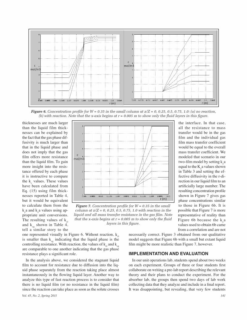
Vol. 45, No. 2, Spring 2011 141
thicknesses are much larger than the liquid film thick-nesses can be explained by the fact that the gas phase dif-fusivity is much larger than that in the liquid phase and does not imply that the gas film offers more resistance than the liquid film. To gain more insight into the resis-tance offered by each phase it is instructive to compare the kc values. These values have been calculated from Eq. (15) using film thick-nesses reported in Table 4, but it would be equivalent to calculate them from the kya and kxa values using ap-propriate unit conversions. The resulting values of kcl and kcg shown in Table 4, tell a similar story to the one represented visually in Figure 6. Without reaction, kcl is smaller than kcg indicating that the liquid phase is the controlling resistance. With reaction, the values of kcl and kcg are comparable to one another indicating that the gas phase resistance plays a significant role.
In the analysis above, we considered the stagnant liquid film to account for resistance due to diffusion into the liq-uid phase separately from the reaction taking place almost instantaneously in the flowing liquid layer. Another way to analyze this type of fast reaction process is to consider that there is no liquid film (or no resistance in the liquid film) since the reaction can take place as soon as the solute crosses
the interface. In that case, all the resistance to mass transfer would be in the gas film and the individual gas film mass transfer coefficient would be equal to the overall mass transfer coefficient. We modeled that scenario in our two-film model by setting kya equal to the Kya values shown in Table 3 and setting the ef-fective diffusivity in the r-di-rection in our liquid film to an artificially large number. The resulting concentration profile shown in Figure 7 gives gas phase concentrations similar to those in Figure 6b. It is possible that Figure 7 is more representative of reality than Figure 6b because the kya values used to obtain 6b came from a correlation and are not
necessarily correct. Figure 3 obtained from our qualitative model suggests that Figure 6b with a small but extant liquid film might be more realistic than Figure 7, however.
IMPLEMENTATION AND EVALUATIONIn our unit operations lab, students spend about two weeks
on each experiment. Groups of three or four students first collaborate on writing a pre-lab report describing the relevant theory and their plans to conduct the experiment. For the absorber lab, the groups then spend two days of lab work collecting data that they analyze and include in a final report. It was disappointing, but revealing, that very few students
Figure 7. Concentration profile for W = 0.35 in the small column at z/Z = 0, 0.25, 0.5, 0.75, 1.0 with reaction in the
liquid and all mass transfer resistance in the gas film. Note that the x-axis begins at r = 0.005 m to show only the fluid
layers in this figure.
Figure 6. Concentration profile for W = 0.35 in the small column at z/Z = 0, 0.25, 0.5, 0.75, 1.0: (a) no reaction, (b) with reaction. Note that the x-axis begins at r = 0.005 m to show only the fluid layers in this figure.
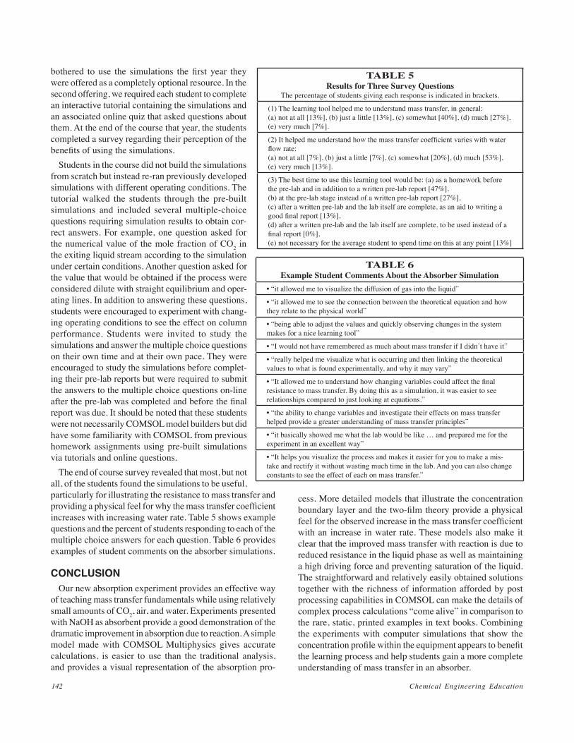
Chemical Engineering Education142
bothered to use the simulations the first year they were offered as a completely optional resource. In the second offering, we required each student to complete an interactive tutorial containing the simulations and an associated online quiz that asked questions about them. At the end of the course that year, the students completed a survey regarding their perception of the benefits of using the simulations.
Students in the course did not build the simulations from scratch but instead re-ran previously developed simulations with different operating conditions. The tutorial walked the students through the pre-built simulations and included several multiple-choice questions requiring simulation results to obtain cor-rect answers. For example, one question asked for the numerical value of the mole fraction of CO2 in the exiting liquid stream according to the simulation under certain conditions. Another question asked for the value that would be obtained if the process were considered dilute with straight equilibrium and oper-ating lines. In addition to answering these questions, students were encouraged to experiment with chang-ing operating conditions to see the effect on column performance. Students were invited to study the simulations and answer the multiple choice questions on their own time and at their own pace. They were encouraged to study the simulations before complet-ing their pre-lab reports but were required to submit the answers to the multiple choice questions on-line after the pre-lab was completed and before the final report was due. It should be noted that these students were not necessarily COMSOL model builders but did have some familiarity with COMSOL from previous homework assignments using pre-built simulations via tutorials and online questions.
The end of course survey revealed that most, but not all, of the students found the simulations to be useful, particularly for illustrating the resistance to mass transfer and providing a physical feel for why the mass transfer coefficient increases with increasing water rate. Table 5 shows example questions and the percent of students responding to each of the multiple choice answers for each question. Table 6 provides examples of student comments on the absorber simulations.
CONCLUSIONOur new absorption experiment provides an effective way
of teaching mass transfer fundamentals while using relatively small amounts of CO2, air, and water. Experiments presented with NaOH as absorbent provide a good demonstration of the dramatic improvement in absorption due to reaction. A simple model made with COMSOL Multiphysics gives accurate calculations, is easier to use than the traditional analysis, and provides a visual representation of the absorption pro-
TABLE 5Results for Three Survey Questions
The percentage of students giving each response is indicated in brackets.
(1) The learning tool helped me to understand mass transfer, in general:(a) not at all [13%], (b) just a little [13%], (c) somewhat [40%], (d) much [27%], (e) very much [7%].
(2) It helped me understand how the mass transfer coefficient varies with water flow rate:(a) not at all [7%], (b) just a little [7%], (c) somewhat [20%], (d) much [53%], (e) very much [13%].
(3) The best time to use this learning tool would be: (a) as a homework before the pre-lab and in addition to a written pre-lab report [47%],(b) at the pre-lab stage instead of a written pre-lab report [27%],(c) after a written pre-lab and the lab itself are complete, as an aid to writing a good final report [13%],(d) after a written pre-lab and the lab itself are complete, to be used instead of a final report [0%],(e) not necessary for the average student to spend time on this at any point [13%]
TABLE 6Example Student Comments About the Absorber Simulation
• “it allowed me to visualize the diffusion of gas into the liquid”
• “it allowed me to see the connection between the theoretical equation and how they relate to the physical world”
• “being able to adjust the values and quickly observing changes in the system makes for a nice learning tool”
• “I would not have remembered as much about mass transfer if I didn’t have it”
• “really helped me visualize what is occurring and then linking the theoretical values to what is found experimentally, and why it may vary”
• “It allowed me to understand how changing variables could affect the final resistance to mass transfer. By doing this as a simulation, it was easier to see relationships compared to just looking at equations.”
• “the ability to change variables and investigate their effects on mass transfer helped provide a greater understanding of mass transfer principles”
• “it basically showed me what the lab would be like … and prepared me for the experiment in an excellent way”
• “It helps you visualize the process and makes it easier for you to make a mis-take and rectify it without wasting much time in the lab. And you can also change constants to see the effect of each on mass transfer.”
cess. More detailed models that illustrate the concentration boundary layer and the two-film theory provide a physical feel for the observed increase in the mass transfer coefficient with an increase in water rate. These models also make it clear that the improved mass transfer with reaction is due to reduced resistance in the liquid phase as well as maintaining a high driving force and preventing saturation of the liquid. The straightforward and relatively easily obtained solutions together with the richness of information afforded by post processing capabilities in COMSOL can make the details of complex process calculations “come alive” in comparison to the rare, static, printed examples in text books. Combining the experiments with computer simulations that show the concentration profile within the equipment appears to benefit the learning process and help students gain a more complete understanding of mass transfer in an absorber.
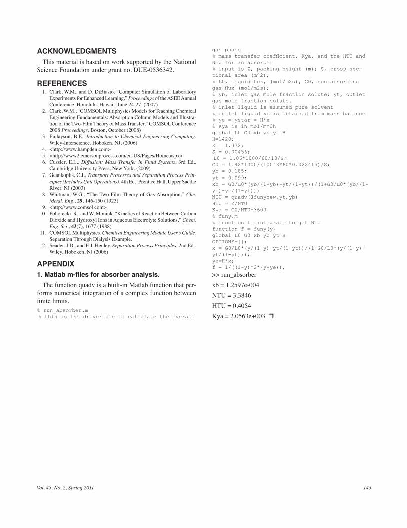
Vol. 45, No. 2, Spring 2011 143
ACKNOWLEDGMENTSThis material is based on work supported by the National
Science Foundation under grant no. DUE-0536342.
REFERENCES 1. Clark, W.M., and D. DiBiasio, “Computer Simulation of Laboratory
Experiments for Enhanced Learning,” Proceedings of the ASEE Annual Conference, Honolulu, Hawaii, June 24-27, (2007)
2. Clark, W.M., “COMSOL Multiphysics Models for Teaching Chemical Engineering Fundamentals: Absorption Column Models and Illustra-tion of the Two-Film Theory of Mass Transfer,” COMSOL Conference 2008 Proceedings, Boston, October (2008)
3. Finlayson, B.E., Introduction to Chemical Engineering Computing, Wiley-Interscience, Hoboken, NJ, (2006)
4. <http://www.hampden.com> 5. <http://www2.emersonprocess.com/en-US/Pages/Home.aspx> 6. Cussler, E.L., Diffusion: Mass Transfer in Fluid Systems, 3rd Ed.,
Cambridge University Press, New York, (2009) 7. Geankoplis, C.J., Transport Processes and Separation Process Prin-
ciples (Includes Unit Operations), 4th Ed., Prentice Hall, Upper Saddle River, NJ (2003)
8. Whitman, W.G., “The Two-Film Theory of Gas Absorption,” Che. Metal. Eng., 29, 146-150 (1923)
9. <http://www.comsol.com> 10. Pohorecki, R., and W. Moniuk, “Kinetics of Reaction Between Carbon
Dioxide and Hydroxyl Ions in Aqueous Electrolyte Solutions,” Chem. Eng. Sci., 43(7), 1677 (1988)
11. COMSOL Multiphysics, Chemical Engineering Module User’s Guide, Separation Through Dialysis Example.
12. Seader, J.D., and E.J. Henley, Separation Process Principles, 2nd Ed., Wiley, Hoboken, NJ (2006)
APPENDIX 1. Matlab m-files for absorber analysis.
The function quadv is a built-in Matlab function that per-forms numerical integration of a complex function between finite limits.% run_absorber.m%thisisthedriverfiletocalculatetheoverall
gas phase%masstransfercoefficient,Kya,andtheHTUandNTUforanabsorber%inputisZ,packingheight(m);S,crosssec-tionalarea(m^2);%L0,liquidflux,(mol/m2s),G0,nonabsorbinggasflux(mol/m2s);%yb,inletgasmolefractionsolute;yt,outletgasmolefractionsolute.%inletliquidisassumedpuresolvent%outletliquidxbisobtainedfrommassbalance%ye=ystar=H*x%Kyaisinmol/m^3hglobalL0G0xbybytHH=1420;Z=1.372;S=0.00456;L0=1.06*1000/60/18/S;G0=1.42*1000/(100^3*60*0.022415)/S;yb=0.185;yt=0.099;xb=G0/L0*(yb/(1-yb)-yt/(1-yt))/(1+G0/L0*(yb/(1-yb)-yt/(1-yt)))NTU=quadv(@funynew,yt,yb)HTU=Z/NTUKya=G0/HTU*3600%funy.m%functiontointegratetogetNTUfunctionf=funy(y)globalL0G0xbybytHOPTIONS=[];x=G0/L0*(y/(1-y)-yt/(1-yt))/(1+G0/L0*(y/(1-y)-yt/(1-yt)));ye=H*x;f=1/((1-y)^2*(y-ye));
>> run_absorberxb = 1.2597e-004NTU = 3.3846HTU = 0.4054Kya = 2.0563e+003 p
Chemical Engineering Education144
Optimization is often considered to be an advanced, highly mathematical, and sometimes a somewhat obscure discipline. While it is true that many ad-
vanced optimization techniques exist, optimization problems can be developed that are suitable for undergraduates at all levels. Two of these problems will be described in this paper, and many others are available on the web.[1] A pedagogy is described that requires students to identify the trends of the components of the objective function and to understand how trade-offs between these components lead to the existence of the optimum.
The ability to solve “routine” optimization problems has been simplified by advances in computing power over the last generation. Earlier editions of current design textbooks[2] presented a sequence of optimization techniques aimed at minimizing the number of cases that had to be considered to close in on the optimum. Now, it is possible to perform optimization calculations involving numerous cases with a few clicks of a mouse, and an entire chemical process can be simulated and results exported to a spreadsheet in a matter of minutes.
Several optimization examples are routinely discussed in undergraduate textbooks; however, the objective func-tion does not usually involve economics. These examples include optimum interstage compressor pressure,[3] optimum insulation thickness,[4] and identifying conditions for the optimum selectivity.[5] Qualitative representations of the
economic optimum pipe diameter[6] and reflux ratio[7] are also available. Other examples of optimization problems are available, but these do not involve an economic objec-tive function.[8-10] The problems presented here all involve an economic objective function.
TYPES OF PROBLEMS Three types of optimization problems are available, and
they are summarized in Table 1. The ones highlighted in ital-ics are discussed in this paper, and the others are available on the web.[1] The numbers in parenthesis indicate the number of different versions available for each problem. All of these have been used successfully in a freshman class designed to develop computing skills appropriate for an undergraduate chemical engineering student. Most of these problems would also be suitable for assignments or projects in unit operations
OPTIMIZATION PROBLEMSBrian J. andErSon, roBin S. hiSSam, JoSEph a. ShaEiWitz, and riChard turton
West Virginia University • Morgantown, WV 26506-6102
Brian J. Anderson is the Verl Purdy Faculty Fellow and an assistant professor in the Department of Chemical Engineering at West Virginia University. His research experience includes sustainable energy and development, economic modeling of energy systems, and geothermal energy development as well as molecular and reservoir modeling.
Robin S. Hissam received her B.S. and M.S. degrees in materials science and engineering from Virginia Tech and her Ph.D. in materials science and engineer-ing from the University of Delaware. After a post-doctoral fellowship in chemical engineering and applied chemistry at the University of Toronto, Robin joined the Chemical Engineering Department at West Virginia University. Her research is in production of protein polymers for application in tissue engineering, biomin-eralization, and biosensors. © Copyright ChE Division of ASEE 2011
TABLE 1Available Optimization Problems
Single Variable
Multi-variable Projects
Pipe diam-eter (2)
Absorber Generic chemical process (2)
Reactor/preheater (2)
Batch reactor/pre-heater
Geothermal energy (2)
Reflux ratio Staged compressors Fuel production from biomass (4)
ChE class and home problems
Joseph A. Shaeiwitz received his B.S. degree from the University of Delaware and his M.S. and Ph.D. degrees from Carnegie Mellon University. His profes-sional interests are in design, design education, and outcomes assessment. Joe is a co-author of the text Analysis, Synthesis, and Design of Chemical Processes (3rd Ed.), published by Prentice Hall in 2009.
Richard Turton, P.E., has taught the senior design course at West Virginia University for the past 24 years. Prior to this, he spent five years in the design and construction industry. His main interests are in design education, particulate processing, and modeling of advanced energy processes. Richard is a co-author of the text Analysis, Synthesis, and Design of Chemical Processes (3rd Ed.), published by Prentice Hall in 2009.
The object of this column is to enhance our readers’ collections of interesting and novel problems in chemical engineering. We request problems that can be used to motivate student learning by presenting a particular principle in a new light, can be assigned as novel home problems, are suited for a collaborative learning environment, or dem-onstrate a cutting-edge application or principle. Manuscripts should not exceed 14 double-spaced pages and should be accompanied by the originals of any figures or photographs. Please submit them to Dr. Daina Briedis (e-mail: [email protected]), Department of Chemical Engineering and Materials Science, Michigan State University, East Lansing, MI 48824-1226.
Vol. 45, No. 2, Spring 2011 145
classes or as problem assignments for the portion of a design class where optimization is taught.
Problem 1: Bioreactor Background
A liquid-phase, biological reaction is used to produce an intermediate chemical for use in the pharmaceutical indus-try. The reaction occurs in a large, well-stirred, isothermal bioreactor, such that the reactor temperature is identical to the inlet temperature. Because this chemical is temperature sensitive, the maximum operating temperature in the reactor is limited to 65 ̊ C by using a heating medium available at this maximum temperature. The feed material is fed to the reactor through a heat exchanger that can increase the temperature of the reactants (contents of the reactor), which in turn increases the rate of the reaction. This is illustrated in Figure 1. The time spent in the bioreactor (known as the space time) must be adjusted to obtain the desired conversion of reactant. As the temperature in the reactor increases so does the reaction rate, thereby decreasing the size (and cost) of the reactor required to give the desired conversion. The problem to be solved is to determine the optimal value for the single independent variable; namely, the temperature (Tc,2) at which to maintain the reactor (preheat the feed). The costs to be considered are the purchase costs of the reactor and heat exchanger and the operating cost for the energy to heat the feed. Problem Statement
It is desired to optimize the preheat temperature for a re-actant feed flow of 5,000 gal/h. The feed has the properties of water ( ρ = 1,000 kg/m3, Cp = 4.18 kJ/kg ˚C) and enters the heat exchanger at a temperature of 20 ˚C. The reactor feed is to be heated with a heating medium that is available at a temperature of 65 ˚C and must leave the heat exchanger at 30 ˚C. Therefore, the desired reactor inlet temperature is adjusted by changing the flowrate of the heating medium. The physical properties of the heating medium are ρ = 920 kg/m3, Cp = 2.2 kJ/kg ˚C.
The reaction rate for this reaction, –rA, is given in terms of the concentration of reactant A (CA) by the following equation:
− =r kCA A ( )1 where
k sT K
− = −
1 2 5 3 500 2. exp , ( ))
The design equation for the reactor is given by:
Vv X
k Xo A
A
=−( )1
3( )
where V is the reactor volume (m3), vo is the volumetric flow-rate of fluid into the reactor (m3/s), and XA is the conversion (assumed to be 80% or 0.8 for this reaction).
The design equation for the heat exchanger is given by:
Q M C T T M C T T UAF Tc p c c c h p h h h= ( )= ( )=− − ∆, , , , , ,2 1 1 2 llm ( )4
where
∆ =−( )− −( )
−( )T
T T T T
T T
T
lmh c h c
h c
h
, , , ,
, ,ln
2 1 1 2
2 1
,, ,
( )
1 2
5
−( )Tc
and F = log-mean temperature correction factor = 0.8 (assume
that this is constant for all cases) U = overall heat transfer coefficient = 400 W/m2K The optimum reactor inlet temperature is the one that
minimizes the equivalent annual operating cost (EAOC). The EAOC is given by
EAOC y PC A P i n yii
$ / $ / , , / =
( )
=∑1
2
1 +
UC y$ / ( )6
where PCi are the purchase equipment costs for the heat exchanger and reactor, UC is the operating (utility) cost for the heating medium, and (A/P, i, n) is the capital recovery factor given by
A P i ni i
i
n
n/ , , ( )( )=
+( )+( ) −1
1 17
For this problem, use i = 7% and n = 12 years. The purchase cost of the reactor is given by:
PC Vreactor = $ , ( ).17 000 80 85
where V is the volume of the reactor in m3. The cost of the heat exchanger is:
PC A mexchanger ={ }$ , ( )
.12 000 92
0 57
where A is the area of the heat exchanger in m2. The cost of the heating medium is:
UC h Q kJ h$ / $ / ( ) = ×
5 10 106
Figure 1. Process flow diagram of the feed preheater and bioreactor.
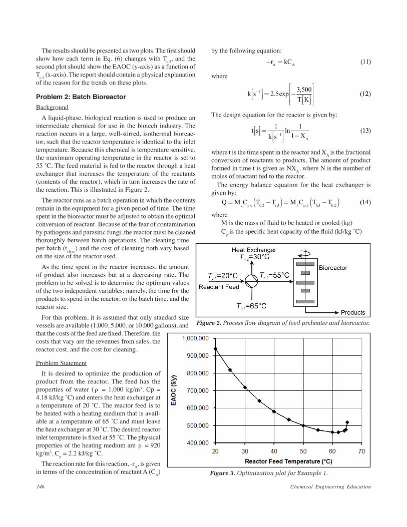
Chemical Engineering Education146
The results should be presented as two plots. The first should show how each term in Eq. (6) changes with Tc,2, and the second plot should show the EAOC (y-axis) as a function of Tc,2 (x-axis). The report should contain a physical explanation of the reason for the trends on these plots.
Problem 2: Batch Bioreactor Background
A liquid-phase, biological reaction is used to produce an intermediate chemical for use in the biotech industry. The reaction occurs in a large, well-stirred, isothermal bioreac-tor, such that the reactor temperature is identical to the inlet temperature. Because this chemical is temperature sensitive, the maximum operating temperature in the reactor is set to 55 ˚C. The feed material is fed to the reactor through a heat exchanger that increases the temperature of the reactants (contents of the reactor), which in turn increases the rate of the reaction. This is illustrated in Figure 2.
The reactor runs as a batch operation in which the contents remain in the equipment for a given period of time. The time spent in the bioreactor must be adjusted to obtain the optimal conversion of reactant. Because of the fear of contamination by pathogens and parasitic fungi, the reactor must be cleaned thoroughly between batch operations. The cleaning time per batch (tclean) and the cost of cleaning both vary based on the size of the reactor used.
As the time spent in the reactor increases, the amount of product also increases but at a decreasing rate. The problem to be solved is to determine the optimum values of the two independent variables; namely, the time for the products to spend in the reactor, or the batch time, and the reactor size.
For this problem, it is assumed that only standard size vessels are available (1,000, 5,000, or 10,000 gallons), and that the costs of the feed are fixed. Therefore, the costs that vary are the revenues from sales, the reactor cost, and the cost for cleaning.
Problem Statement It is desired to optimize the production of
product from the reactor. The feed has the properties of water ( ρ = 1,000 kg/m3, Cp = 4.18 kJ/kg ˚C) and enters the heat exchanger at a temperature of 20 ˚C. The reactor feed is to be heated with a heating medium that is avail-able at a temperature of 65 ˚C and must leave the heat exchanger at 30 ̊ C. The desired reactor inlet temperature is fixed at 55 ̊ C. The physical properties of the heating medium are ρ = 920 kg/m3, Cp = 2.2 kJ/kg ˚C.
The reaction rate for this reaction, -rA, is given in terms of the concentration of reactant A (CA)
by the following equation:
− =r kCA A ( )11
where
k sT K
− = −
1 2 5 3 500 1. exp , ( 22)
The design equation for the reactor is given by:
t sk s XA
=
−−
1 11
131
ln ( )
where t is the time spent in the reactor and XA is the fractional conversion of reactants to products. The amount of product formed in time t is given as NXA, where N is the number of moles of reactant fed to the reactor.
The energy balance equation for the heat exchanger is given by:
Q M C T T M C T Tc p c c c h p h h h= −( )= −( ), , , , , , ( )2 1 1 2 14
where M is the mass of fluid to be heated or cooled (kg) Cp is the specific heat capacity of the fluid (kJ/kg ˚C)
Figure 2. Process flow diagram of feed preheater and bioreactor.
Figure 3. Optimization plot for Example 1.
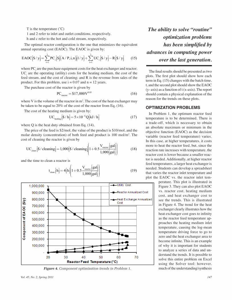
Vol. 45, No. 2, Spring 2011 147
The final results should be presented as two plots. The first plot should show how each term in Eq. (15) changes with the batch time, t, and the second plot should show the EAOC (y- axis) as a function of t (x-axis). The report should contain a physical explanation of the reason for the trends on these plots.
OPTIMIZATION PROBLEMS In Problem 1, the optimum reactor feed
temperature is to be determined. There is a trade-off, which is necessary to obtain an absolute maximum or minimum in the objective function (EAOC) as the decision variable (reactor feed temperature) varies. In this case, at higher temperatures, it costs more to heat the reactor feed, but, since the reaction rate increases with temperature, the reactor cost is lower because a smaller reac-tor is needed. Additionally, at higher reactor feed temperatures, a larger heat exchanger is needed. Students can develop a spreadsheet that varies the reactor inlet temperature and plot the EAOC vs. the reactor inlet tem-
perature. This plot is illustrated in Figure 3. They can also plot EAOC vs. reactor cost, heating medium cost, and heat exchanger cost to see the trends. This is illustrated in Figure 4. The trend for the heat exchanger clearly illustrates how the heat exchanger cost goes to infinity as the reactor feed temperature ap-proaches the heating medium inlet temperature, causing the log-mean temperature driving force to go to zero and the heat exchanger area to become infinite. This is an example of why it is important for students to analyze a series of data and un-derstand the trends. It is possible to solve this entire problem on Excel using the Solver tool; however, much of the understanding/synthesis Figure 4. Component optimization trends in Problem 1.
T is the temperature (˚C) 1 and 2 refer to inlet and outlet conditions, respectively. h and c refer to the hot and cold stream, respectively.
The optimal reactor configuration is the one that minimizes the equivalent annual operating cost (EAOC). The EAOC is given by:
EAOC y PC A P i n yii
$ / $ / , , / =
( )
=∑1
2
1 +
−
=∑UC y R yii 1
3
15$ / $ / ( )
where PCi are the purchase equipment costs for the heat exchanger and reactor; UCi are the operating (utility) costs for the heating medium, the cost of the feed stream, and the cost of cleaning; and R is the revenue from sales of the product. For this problem, use i = 0.07 and n = 12 years.
The purchase cost of the reactor is given by PC Vreactor = $ , ( ).17 000 160 85
where V is the volume of the reactor in m3. The cost of the heat exchanger may be taken to be equal to 20% of the cost of the reactor from Eq. (16).
The cost of the heating medium is given by: UC h Q kJ hheating $ / / ( )
= ×
−5 10 176
where Q is the heat duty obtained from Eq. (14). The price of the feed is $2/mol, the value of the product is $10/mol, and the
molar density (concentration) of both feed and product is 100 mol/m3. The cost of cleaning the reactor is given by
UC cleaning cleaningclean $ / , $ /
=
1 000 +
1 0 51 000
.,
V gal
galreactor
( )18
and the time to clean a reactor is
t h hV gal
cleanreactor
=
+
4 1 0 5.
1 00019
,( )
gal
The ability to solve “routine” optimization problems has been simplified by
advances in computing power over the last generation.
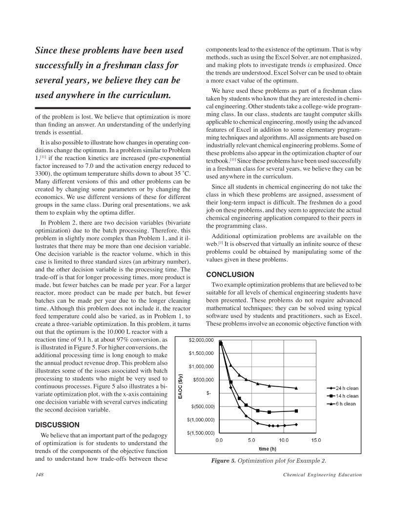
Chemical Engineering Education148
of the problem is lost. We believe that optimization is more than finding an answer. An understanding of the underlying trends is essential.
It is also possible to illustrate how changes in operating con-ditions change the optimum. In a problem similar to Problem 1,[11] if the reaction kinetics are increased (pre-exponential factor increased to 7.0 and the activation energy reduced to 3300), the optimum temperature shifts down to about 35 ˚C. Many different versions of this and other problems can be created by changing some parameters or by changing the economics. We use different versions of these for different groups in the same class. During oral presentations, we ask them to explain why the optima differ.
In Problem 2, there are two decision variables (bivariate optimization) due to the batch processing. Therefore, this problem in slightly more complex than Problem 1, and it il-lustrates that there may be more than one decision variable. One decision variable is the reactor volume, which in this case is limited to three standard sizes (an arbitrary number), and the other decision variable is the processing time. The trade-off is that for longer processing times, more product is made, but fewer batches can be made per year. For a larger reactor, more product can be made per batch, but fewer batches can be made per year due to the longer cleaning time. Although this problem does not include it, the reactor feed temperature could also be varied, as in Problem 1, to create a three-variable optimization. In this problem, it turns out that the optimum is the 10,000 L reactor with a reaction time of 9.1 h, at about 97% conversion, as is illustrated in Figure 5. For higher conversions, the additional processing time is long enough to make the annual product revenue drop. This problem also illustrates some of the issues associated with batch processing to students who might be very used to continuous processes. Figure 5 also illustrates a bi-variate optimization plot, with the x-axis containing one decision variable with several curves indicating the second decision variable.
DISCUSSION We believe that an important part of the pedagogy
of optimization is for students to understand the trends of the components of the objective function and to understand how trade-offs between these
components lead to the existence of the optimum. That is why methods, such as using the Excel Solver, are not emphasized, and making plots to investigate trends is emphasized. Once the trends are understood, Excel Solver can be used to obtain a more exact value of the optimum.
We have used these problems as part of a freshman class taken by students who know that they are interested in chemi-cal engineering. Other students take a college-wide program-ming class. In our class, students are taught computer skills applicable to chemical engineering, mostly using the advanced features of Excel in addition to some elementary program-ming techniques and algorithms. All assignments are based on industrially relevant chemical engineering problems. Some of these problems also appear in the optimization chapter of our textbook.[11] Since these problems have been used successfully in a freshman class for several years, we believe they can be used anywhere in the curriculum.
Since all students in chemical engineering do not take the class in which these problems are assigned, assessment of their long-term impact is difficult. The freshmen do a good job on these problems, and they seem to appreciate the actual chemical engineering application compared to their peers in the programming class.
Additional optimization problems are available on the web.[1] It is observed that virtually an infinite source of these problems could be obtained by manipulating some of the values given in these problems.
CONCLUSION Two example optimization problems that are believed to be
suitable for all levels of chemical engineering students have been presented. These problems do not require advanced mathematical techniques; they can be solved using typical software used by students and practitioners, such as Excel. These problems involve an economic objective function with
Figure 5. Optimization plot for Example 2.
Since these problems have been used successfully in a freshman class for several years, we believe they can be used anywhere in the curriculum.
Vol. 45, No. 2, Spring 2011 149
component capital and operating cost terms. An important part of the pedagogy of these problems is an understanding of how the trends of the components terms in the objective function contribute to the trade-off involved in most optimi-zation problems.
REFERENCES 1. <http://www.che.cemr.wvu.edu/publications/projects/index.
php#opt> 2. Peters, M.S., and K.D. Timmerhaus, Plant Design and Economics for
Chemical Engineers, (3rd Ed.), McGraw Hill, New York, 1980, Chapter 10
3. Sandler, S.I., Chemical, Biochemical, and Engineering Thermodynam-ics (4th Ed.), Wiley, New York, 2006, Chapter 4, Problem 4.21b
4. Geankoplis, C., Transport Processes and Separation Principles (4th
Ed.), Prentice Hall PTR, Upper Saddle River, NJ, 2003, Chapter 4.3F 5. Fogler, H.S., Elements of Chemical Reaction Engineering (4th Ed.),
Prentice Hall PTR, Upper Saddle River, NJ, 2006, Chapter 6 6. de Nevers, N., Fluid Mechanics for Chemical Engineers (3rd Ed.),
McGraw Hill, New York, 2005, Chapter 6 7. Peters, M.S., K.D. Timmerhaus, and R.E. West, Plant Design and
Economics for Chemical Engineers, (4th Ed.), McGraw Hill, New York, 2003, Chapter 9
8. Barolo, M., “Batch Distillation Optimization Made Easy,” Chem. Eng. Ed., 32(4), 280 (1998)
9. Smart, J., “Using the Evolutionary Method to Optimize Gas Absorber Operation,” Chem. Eng. Ed., 38(3), 204 (2004)
10. Mitsos, A., “Design Course for Micropower Generation Devices,” Chem. Eng. Ed., 43(3), 201 (2009)
11. Turton, R., R.C. Bailie, W.B. Whiting, and J.A. Shaeiwitz, Analysis, Synthesis, and Design of Chemical Processes (3rd Ed.), Prentice Hall PTR, Upper Saddle River, NJ, 2009, Chapter 14 p
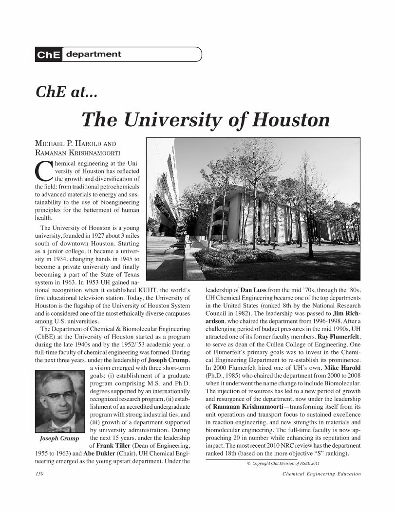
Chemical Engineering Education150
ChE department
ChE at...
The University of Houston
Chemical engineering at the Uni-versity of Houston has reflected the growth and diversification of
the field: from traditional petrochemicals to advanced materials to energy and sus-tainability to the use of bioengineering principles for the betterment of human health.
The University of Houston is a young university, founded in 1927 about 3 miles south of downtown Houston. Starting as a junior college, it became a univer-sity in 1934, changing hands in 1945 to become a private university and finally becoming a part of the State of Texas system in 1963. In 1953 UH gained na-tional recognition when it established KUHT, the world’s first educational television station. Today, the University of Houston is the flagship of the University of Houston System and is considered one of the most ethnically diverse campuses among U.S. universities.
The Department of Chemical & Biomolecular Engineering (ChBE) at the University of Houston started as a program during the late 1940s and by the 1952/’53 academic year, a full-time faculty of chemical engineering was formed. During the next three years, under the leadership of Joseph Crump,
a vision emerged with three short-term goals: (i) establishment of a graduate program comprising M.S. and Ph.D. degrees supported by an internationally recognized research program, (ii) estab-lishment of an accredited undergraduate program with strong industrial ties, and (iii) growth of a department supported by university administration. During the next 15 years, under the leadership of Frank Tiller (Dean of Engineering,
1955 to 1963) and Abe Dukler (Chair), UH Chemical Engi-neering emerged as the young upstart department. Under the
leadership of Dan Luss from the mid ’70s, through the ’80s, UH Chemical Engineering became one of the top departments in the United States (ranked 8th by the National Research Council in 1982). The leadership was passed to Jim Rich-ardson, who chaired the department from 1996-1998. After a challenging period of budget pressures in the mid 1990s, UH attracted one of its former faculty members, Ray Flumerfelt, to serve as dean of the Cullen College of Engineering. One of Flumerfelt’s primary goals was to invest in the Chemi-cal Engineering Department to re-establish its prominence. In 2000 Flumerfelt hired one of UH’s own, Mike Harold (Ph.D., 1985) who chaired the department from 2000 to 2008 when it underwent the name change to include Biomolecular. The injection of resources has led to a new period of growth and resurgence of the department, now under the leadership of Ramanan Krishnamoorti—transforming itself from its unit operations and transport focus to sustained excellence in reaction engineering, and new strengths in materials and biomolecular engineering. The full-time faculty is now ap-proaching 20 in number while enhancing its reputation and impact. The most recent 2010 NRC review has the department ranked 18th (based on the more objective “S” ranking).
miChaEl p. harold and ramanan KriShnamoorti
Joseph Crump
© Copyright ChE Division of ASEE 2011
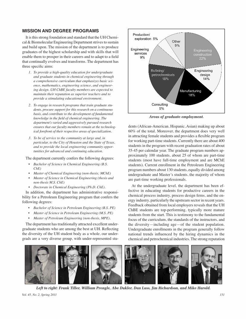
Vol. 45, No. 2, Spring 2011 151
MISSION AND DEGREE PROGRAMSIt is this strong foundation and standard that the UH Chemi-
cal & Biomolecular Engineering Department strives to sustain and build upon. The mission of the department is to produce graduates of the highest scholarship and with skills that will enable them to prosper in their careers and to adapt to a field that continually evolves and transforms. The department has three specific aims:
1. To provide a high-quality education for undergraduate and graduate students in chemical engineering through a comprehensive curriculum that emphasizes basic sci-ence, mathematics, engineering science, and engineer-ing design. UH ChBE faculty members are expected to maintain their reputation as superior teachers and to provide a stimulating educational environment.
2. To engage in research programs that train graduate stu-dents, procure support for this research on a continuous basis, and contribute to the development of fundamental knowledge in the field of chemical engineering. The department’s varied and aggressively pursued research ensures that our faculty members remain at the technolog-ical forefront of their respective areas of specialization.
3. To be of service to the community at large and, in particular, to the City of Houston and the State of Texas, and to provide the local engineering community oppor-tunities for advanced and continuing education.
The department currently confers the following degrees: • Bachelor of Science in Chemical Engineering (B.S.
ChE)• Master of Chemical Engineering (non-thesis; MChE) • Master of Science in Chemical Engineering (thesis and
non-thesis M.S. ChE) • Doctorate in Chemical Engineering (Ph.D. ChE).
In addition, the department has administrative responsi-bility for a Petroleum Engineering program that confers the following degrees:
• Bachelor of Science in Petroleum Engineering (B.S. PE)• Master of Science in Petroleum Engineering (M.S. PE)• Master of Petroleum Engineering (non-thesis, MPE).
The department has traditionally attracted excellent under-graduate students who are among the best at UH. Reflecting the diversity of the UH student body as a whole, our under-grads are a very diverse group, with under-represented stu-
dents (African-American, Hispanic, Asian) making up about 60% of the total. Moreover, the department does very well in attracting female students and provides a flexible program for working part-time students. Currently there are about 400 students in the program with recent graduation rates of about 35-45 per calendar year. The graduate program numbers ap-proximately 100 students, about 25 of whom are part-time students (most have full-time employment and are MChE students). Current enrollment in the Petroleum Engineering program numbers about 130 students, equally divided among undergraduate and Master’s students, the majority of whom are part-time working professionals.
At the undergraduate level, the department has been ef-fective in educating students for productive careers in the chemical process industry, process design firms, and the en-ergy industry, particularly the upstream sector in recent years. Feedback obtained from local employers reveals that the UH ChBE students are top-performing, typically more mature students from the start. This is testimony to the fundamental focus of the curriculum, the standards of the instructors, and the diversity—including age—of the student population. Undergraduate enrollments in the program generally follow national trends influenced by the hiring dynamics in the chemical and petrochemical industries. The strong reputation
Left to right: Frank Tiller, William Prengle, Abe Dukler, Dan Luss, Jim Richardson, and Mike Harold.
Areas of graduate employment.
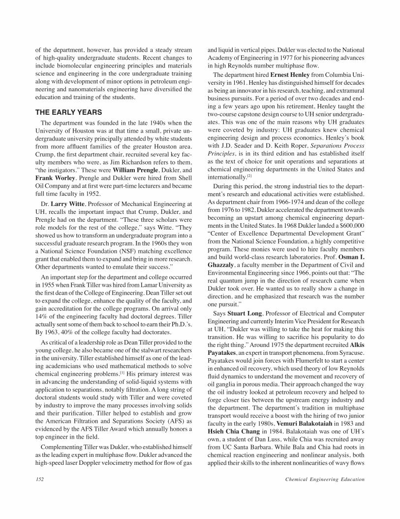
Chemical Engineering Education152
of the department, however, has provided a steady stream of high-quality undergraduate students. Recent changes to include biomolecular engineering principles and materials science and engineering in the core undergraduate training along with development of minor options in petroleum engi-neering and nanomaterials engineering have diversified the education and training of the students.
THE EARLY YEARSThe department was founded in the late 1940s when the
University of Houston was at that time a small, private un-dergraduate university principally attended by white students from more affluent families of the greater Houston area. Crump, the first department chair, recruited several key fac-ulty members who were, as Jim Richardson refers to them, “the instigators.” These were William Prengle, Dukler, and Frank Worley. Prengle and Dukler were hired from Shell Oil Company and at first were part-time lecturers and became full time faculty in 1952.
Dr. Larry Witte, Professor of Mechanical Engineering at UH, recalls the important impact that Crump, Dukler, and Prengle had on the department. “These three scholars were role models for the rest of the college,” says Witte. “They showed us how to transform an undergraduate program into a successful graduate research program. In the 1960s they won a National Science Foundation (NSF) matching excellence grant that enabled them to expand and bring in more research. Other departments wanted to emulate their success.”
An important step for the department and college occurred in 1955 when Frank Tiller was hired from Lamar University as the first dean of the College of Engineering. Dean Tiller set out to expand the college, enhance the quality of the faculty, and gain accreditation for the college programs. On arrival only 14% of the engineering faculty had doctoral degrees. Tiller actually sent some of them back to school to earn their Ph.D.’s. By 1963, 40% of the college faculty had doctorates.
As critical of a leadership role as Dean Tiller provided to the young college, he also became one of the stalwart researchers in the university. Tiller established himself as one of the lead-ing academicians who used mathematical methods to solve chemical engineering problems.[1] His primary interest was in advancing the understanding of solid-liquid systems with application to separations, notably filtration. A long string of doctoral students would study with Tiller and were coveted by industry to improve the many processes involving solids and their purification. Tiller helped to establish and grow the American Filtration and Separations Society (AFS) as evidenced by the AFS Tiller Award which annually honors a top engineer in the field.
Complementing Tiller was Dukler, who established himself as the leading expert in multiphase flow. Dukler advanced the high-speed laser Doppler velocimetry method for flow of gas
and liquid in vertical pipes. Dukler was elected to the National Academy of Engineering in 1977 for his pioneering advances in high Reynolds number multiphase flow.
The department hired Ernest Henley from Columbia Uni-versity in 1961. Henley has distinguished himself for decades as being an innovator in his research, teaching, and extramural business pursuits. For a period of over two decades and end-ing a few years ago upon his retirement, Henley taught the two-course capstone design course to UH senior undergradu-ates. This was one of the main reasons why UH graduates were coveted by industry: UH graduates knew chemical engineering design and process economics. Henley’s book with J.D. Seader and D. Keith Roper, Separations Process Principles, is in its third edition and has established itself as the text of choice for unit operations and separations at chemical engineering departments in the United States and internationally.[2]
During this period, the strong industrial ties to the depart-ment’s research and educational activities were established. As department chair from 1966-1974 and dean of the college from 1976 to 1982, Dukler accelerated the department towards becoming an upstart among chemical engineering depart-ments in the United States. In 1968 Dukler landed a $600,000 “Center of Excellence Departmental Development Grant” from the National Science Foundation, a highly competitive program. These monies were used to hire faculty members and build world-class research laboratories. Prof. Osman I. Ghazzaly, a faculty member in the Department of Civil and Environmental Engineering since 1966, points out that: “The real quantum jump in the direction of research came when Dukler took over. He wanted us to really show a change in direction, and he emphasized that research was the number one pursuit.”
Says Stuart Long, Professor of Electrical and Computer Engineering and currently Interim Vice President for Research at UH, “Dukler was willing to take the heat for making this transition. He was willing to sacrifice his popularity to do the right thing.” Around 1975 the department recruited Alkis Payatakes, an expert in transport phenomena, from Syracuse. Payatakes would join forces with Flumerfelt to start a center in enhanced oil recovery, which used theory of low Reynolds fluid dynamics to understand the movement and recovery of oil ganglia in porous media. Their approach changed the way the oil industry looked at petroleum recovery and helped to forge closer ties between the upstream energy industry and the department. The department’s tradition in multiphase transport would receive a boost with the hiring of two junior faculty in the early 1980s, Vemuri Balakotaiah in 1983 and Hsieh Chia Chang in 1984. Balakotaiah was one of UH’s own, a student of Dan Luss, while Chia was recruited away from UC Santa Barbara. While Bala and Chia had roots in chemical reaction engineering and nonlinear analysis, both applied their skills to the inherent nonlinearities of wavy flows
Vol. 45, No. 2, Spring 2011 153
and flows in porous media, among other systems. During the 1990s the department recruited Kishore Mohanty away from the oil industry. Mohanty would further solidify the ties with the upstream energy industry with his fundamental focus on transport in porous media applied to oil and gas recovery. Complementing Mohanty’s efforts was Michael Economides, hired from Texas A&M in 1998, who brought more practical aspects of petroleum engineering to the program.
THE REACTION ENGINEERING COMPETENCY
The hiring of Luss in 1967 was arguably the most important hire in the department’s 60+ years. Luss, a highly accom-plished student of Neal Amundson at Minnesota, was an expert in chemical reaction engineering. In the same period the department attracted Richardson, an accomplished expert in heterogeneous catalysis, from Exxon. Together their hiring ushered the emergence of chemical reaction engineering as the area in which UH chemical engineering would become the recognized national leader. In 1971, UH attracted Jay Bailey as an assistant professor with primary research inter-est in reaction engineering, and broadened the impact of the pioneering research. Bailey applied the principles of chemical reaction engineering and mathematical methods developed in chemical engineering first to enzyme catalyzed reactions and later to biochemical engineering, becoming one of the pre-eminent biochemical engineers.[3,4]
Luss became chair of the department in 1975, a position that he held until 1996. It was during Luss’ tenure as chair that the department would ascend dramatically, thanks to the seeds planted by Dukler, strategic hires by Luss, and a sustained focus on research excellence in chemical engineering science. Indeed, it was Luss who stunned chemical engineering aca-deme in 1976 when he attracted his former Ph.D. advisor, Neal Amundson, “The Chief,” to Houston. Amundson brought his expertise in applied mathematics and reaction engineering to the department, and proceeded to graduate about 10 more doctoral students during his second career at UH.
Collectively, the department trained a new generation of students who would primarily join industrial research orga-nizations and help to change the way that chemical reactors in particular would be analyzed, modeled, and designed. In the late ’80s the department hired Demetre Economou, an expert in electronic materials processing. Economou helped to bridge the gap between reaction engineering and materials, and has become one of the leading researchers in gas-solid re-actions in plasma processes. In 2000 another of Luss’ students, Mike Harold, was recruited to become the sixth department chair. Harold had established a strong reputation first as an academic at the University of Massachusetts at Amherst, then as a researcher, then a manager at the DuPont Company’s Engineering Research labs at the Experimental Station. Ad-ditional hires included Roy Jackson from Rice in 1977.
In recent years the department has emerged as a leading center for environmental reaction engineering and catalysis. Balakotaiah focused on transport and reaction in catalytic monoliths used in emission aftertreatment systems such as three-way catalytic converters. Harold founded a clean diesel testing and research facility in the early 2000s, now called the Texas Diesel Testing and Research Center and managed by Dr. Charles Rooks who was recruited from industry by Harold. The creation of the diesel center was in response to the regional need to reduce emissions of NOx (NO + NO2) from the exhaust of diesel vehicles and equipment. The Houston area had the dubious distinction of being one of the worst offenders of the Clean Air Act’s ozone standard. Harold at-tracted a City of Houston grant of $4 million to create a diesel vehicle testing facility and a few years later a $12 million grant to expand the operation.
Today Harold and Rooks lead a team of 15 engineers and staff and collaborate with other faculty members in the ChBE and Mechanical Engineering on basic research and technol-ogy development focused on clean diesel. The center has capabilities spanning bench-scale development of emerging technologies to full-scale testing of diesel vehicles. The main focus of the testing activities is on retrofit technolo-gies to decrease NOx and particulate matter emissions from on-road and off-road vehicles and equipment. More recently the department has attracted Jeff Rimer from the University of Delaware, an expert in the synthesis of shape-selective crystalline materials such as zeolites. Rimer and Harold are joining forces to discover new zeolitic materials with enhanced activity and selectivity for the aforementioned lean NOx reduction. Joining the faculty in 2011 will be Bill Epling as an associate professor and Lars Grabow as an assistant professor. Epling, with earlier industrial experience from Cummins, Inc., and an established academic from the University of Waterloo, will be a perfect fit in the department’s efforts in environmental reaction engineering. Grabow brings his expertise in molecular modeling of catalysts to apply to a wide range of problems including environmental reaction engineering, biofuels, electrochemistry and development of a new generation of catalyst materials.
MATERIALS AND BIOTECHNOLOGYMaterials-related research in colloidal, polymeric, and nano
materials along with biotechnology and biomolecular engi-neering have become significant strengths of the department over the last three decades and in part reflect the changing nature of the discipline.
The discovery of high-temperature superconductivity at the University of Houston sparked a materials revolution on campus and the department became a leader in the area of oxide materials. The significant investments in materials characterization, developed in part as a result of the NSF Materials Research Science and Engineering Center, led
Chemical Engineering Education154
to the growth of not only inorganic materials but also to the growth of polymeric and nanoscale materials. In 2002, Vince Donnelly, a leading plasma physics expert, joined the department after two decades at AT&T’s Bell Labs. Since then Donnelly and Economou have established the pre-eminent plasma physics and processing laboratory, with both of them receiving the highest honors from the American Vacuum So-ciety. Michael Nikolaou, an expert in process control, works closely with them to provide robust control for industrial plasma processes.
The proximity of the petrochemical industry and the growth of advanced materials during the last quarter of the 20th century were reflected in the UH Chemical Engineering department’s focus. Starting with Raj Rajagopalan, an expert in colloids recruited from Syracuse in the mid ’80s, and Jay Scheiber, a theoretician working on polymer dynamics, the efforts in soft materials were strengthened by the addition of Ramanan Krishnamoorti and most recently of Manolis Doxastakis, Gila Stein, Jacinta Conrad, and Megan Robertson. These faculty have also led the advancement of nanotechnology research at UH with Krishnamoorti becoming a pioneer in the area of polymer nanocomposites. Doxastakis has developed expertise in applying molecular and multiscale modeling to understand entangled polymers, nanocomposites, and lipid-protein inter-actions. Stein is an expert in polymer thin films, working on developing materials for optoelectronics, advanced optical lithography, and organic photovoltaics. Conrad is studying the interaction between complex fluids such as polymers and colloids and the surfaces that confine or support them with potential applications in petroleum engineering, environmental engineering, and materials engineering. Robertson’s research combines novel synthetic polymer chemistry and elucidation of polymer physics to design nanostructured materials to develop a new generation of materials based on renewable resources and in some cases with biomedical applications. Additionally, the development of a ~ 4000 ft2 class 10/100 nanofabrication facility at UH has enabled the rapid growth of nanoscale soft materials research. Ongoing research to develop advanced materials for energy applications including improved hydro-carbon recovery, solar energy capture, and wind energy—along with a focus on sustainability by using natural biodegradable alternatives to petroleum-based materials—is representative of the efforts of the department to address many of the grand challenges facing humanity.
The growth of the Texas Medical Center over the last 30 years, starting from the pioneering efforts to produce the first artificial heart to the latest innovations in treating cancer, has triggered growth of biomolecular and biochemical engineering in the department. Jay Bailey’s evolution from chemical reaction engineer to the pre-eminent biochemical engineer by the time he left UH in 1980, was the precursor for the current growth in biomolecular research in the department. Richard Willson, an
expert in biomolecular recognition and nucleic acid purifica-tion, joined the department in the late ’80s and is currently the theme leader for the diagnostics thrust of the NIH Western Regional Center of Excellence. Along with Mike Nikolaou (drug delivery), Peter Vekilov (an expert in phase transitions that occur in protein solutions with implications for deadly diseases including sickle cell anemia and Alzheimer’s and for pharmaceutical drug preparation), and most recently Navin Varadarajan (quantifying functional human immune re-sponses by integrated single cell analysis and developing new cancer therapeutics and vaccines) and Patrick Cirino (protein and metabolic engineering and biocatalysis toward cost-effec-tive “green” chemistry and renewable fuels, bioremediation, and “next-generation” therapeutics), the department is well-positioned to grow biomolecular research and find solutions to challenging issues involving human health.
FEATURES AND OUTLOOKThe unique location of the University of Houston and the
close relationship between the petroleum, petro-chemical, and materials industry along with the relation with NASA and, more recently, advanced materials companies and the Texas Medical Center, have positioned the department to be at the forefront of chemical engineering. The department has a unique relationship with the chemical industry and medical center through the graduate and research programs as well as the industrial advisory board. The continued vitality of the short course on heterogeneous catalysis and the significant in-terest in the short course on polymers, along with the renewed interest in the MChE program for working professionals and the significant interest in the part-time Ph.D. program (with doctoral candidates working in the numerous research and development centers in the greater Houston area), demonstrate the close relationship.
These strategic partnerships will continue to drive the suc-cess of the students and faculty of the Department of Chemical and Biomolecular Engineering at the University of Houston. The analytical, quantitative, and systems-based approach that was pioneered by Tiller, Dukler, Amundson, and Luss will continue to be the hallmark of the research performed at UH and will be integrated into the developments in cutting-edge applications in materials, human health, and energy. These will also help shape our evolving undergraduate and graduate curricula and maintain excellence in our teaching, service, and research missions.
REFERENCES 1. Yelshin, A., Filtration & Separation, 29, 37 2. Seader, J.D., K. Henley, and D. Roper, Separation Process Principles,
3rd Ed., Wiley (2011) 3. Bailey, J.E., and D.F. Olis, Biochemical Engineering Fundamentals,
McGraw-Hill, Inc., New York (1986) 4. Reardon, K.F., K.H. Lee, K.D. Wittrup, and V. Hatzimanikatis, Bio-
technology and Bioengineering 2002, 79, 484 p
Vol. 45, No. 2, Spring 2011 155
ChE book reviews
An Introduction to Granular Flowby K. Rao and P. NottCambridge (2009) $155.00
Reviewed byKimberly H. HenthornRose-Hulman Institute of Technology
Granular flows are ubiquitous in nature and industry, particularly in systems involving food, pharmaceutical, and chemical processes. Although it is extremely important to be able to characterize and model these systems, granular flow behavior is still not well-understood. A number of theoreti-cal and empirical models have been proposed to describe the behavior of particulate systems, but there is still much room for refinement. This book gives a solid discussion of a broad range of topics related to granular flow, with much emphasis on theoretical modeling. The authors focus on continuum models, although there is some attention to discrete models as well. Overall, the book is well-written and provides a thorough overview of the current state of granular flow research.
The book begins with an introduction that previews a large number of areas including interparticle forces, packing, granu-lar statics and flow, and modeling, with most of these topics covered in more detail in subsequent chapters. The authors do a good job of briefly describing each of these topics, and offer a lot of external references for further consideration. In my opinion, this chapter could easily be broken into two chapters, with the modeling sections discussed separately, in order to better organize the material. Some portions are a bit choppy and incomplete because too much information is presented at once. Dividing the material and adding more detail in certain places would definitely help with this.
The rest of the book delves into a detailed theoretical discussion of slow plane and three-dimensional flows, flows through hoppers and bunkers, and rapid flows. The material seemed a little unorganized and incomplete in places, and I was disappointed with the quality and placement of many of the figures and tables. I think the authors did an especially good job with Chapter 6 (Flow through Axisymmetric Hop-pers and Bunkers), however. They provided a good mix of theory and experimental data, and I thought their figures in this section were interesting and useful.
Since most of the material is based on complex theories, the authors offer several appendices that provide a basic math-ematics review. Operations with vectors and tensors, a brief analysis of the stress tensor, and methods to evaluate common integrals are a few topics covered here. I was very happy to see these appendices, because the authors assume the readers have a good understanding of advanced mathematics when discussing the material in the main portion of the text.
Each chapter ends with a set of practice problems. These problems were challenging but appropriate for the material in each section. It was interesting to note that many of the prob-lems were adapted from other sources. I especially appreciated that each problem was labeled with a heading that described what concept was being tested. I am not sure if the authors offer a solutions manual for this textbook, but it would certainly be useful for instructors adopting the book for a course.
I disagree with the authors when they state that this book is appropriate for advanced undergraduates or beginning gradu-ate students, at least in the chemical engineering discipline. The material is presented at a much higher level than what I would expect an undergraduate chemical engineering student to be able to handle. The amount of mathematics and model-ing background required to understand the material and the authors’ use of specialized vocabulary makes this book more appropriate for graduate students concentrating in particle technology related fields. I would recommend students first take an introductory particle technology course using an inter-mediate text such as Rhodes1 so that they are better prepared for the material presented in this book.
My comments about the incompleteness of certain topics stem from the overwhelming amount of information available on granular flows. It would be impossible to cover everything without developing a series of texts about the topic. My overall impression of An Introduction to Granular Flow, however, is very positive, and I commend the authors for providing a solid reference for those interested in granular flows. They do a nice job of summarizing peripheral topics while going into the appropriate detail in their focus areas. 1 Rhodes, Introduction to Particle Technology, John Wiley & Sons, 2nd
ed., 2008
Good Mentoring: Fostering Excellent Practice in Higher Educationby Jeanne Nakamura and David J Shernoff with Charles H. HookerJosey-Bass, 303 pages, $40 (2009)
Reviewed byJoseph H. HollesUniversity of Wyoming
Is good mentoring in the genes? Can successful mentors automatically transmit their knowledge, skills, and values to the next generation of students? If so, how can these at-tributes be transmitted in a way that is most useful to their academic offspring? In an effort to better understand “how to keep what has been learned from being lost” Good Mentoring examines three lineages of scientists and the ability of their skills, values, and practices to be transmitted to their students and successive generations.
The general question that the authors are seeking to address is: “Can one generation’s ‘good workers’ nurture similar com-
Chemical Engineering Education156
mitments in members of the next generation even as changing sociocultural conditions pose new challenges to the pursuit of excellence and ethics in a field?” Included in this question was a particular emphasis on the transmission of orienting values and principles uniting excellence with responsible practice. The authors postulate that “the best chance for their cultivation is likely to lie with teachers who embody these values and practices and the learning environments that the teachers create.” Since graduate science education has a strong reliance on learning by apprenticeship, it is an ideal situation for examining mentoring of future generations.
While the subtitle is “Fostering Excellent Practice in Higher Education,” the book is most relevant to a smaller subset of higher ed. In particular, the focus of the book is effective mentoring for supervisors in research. While the case studies focus on mentoring of graduate students and post-doctoral re-searchers in academia, the same outcomes are also applicable in any research mentoring situation including undergraduate researchers, government, or industrially sponsored research laboratories. Finally, both mentors and their students can gain insight into successful relationships from this work.
Good Mentoring is divided into three distinct parts. Part One presents case studies of each of the three lineages. Part Two summarizes the transmission of knowledge, practices, and values across the mentoring generations. Part Three then summarizes the key lessons learned and draws out implica-tions for practitioners and researchers.
In Part One, the authors examine three scientists and their lineages through the second and third generation of academic offspring. In perhaps a bit of irony, all three of these academic lineages are in the field of genetics. The goal of these chapters is to provide a qualitative view of the approaches of each sci-entist towards successful research and mentoring. Subsequent discussion of second and third generations then provides insight into what knowledge was successfully passed down. From these second- and third-generation profiles, we also obtain some insight into how individual scientists affected the overall memes (building blocks of culture) of the lineage.
In Part Two, the authors take a quantitative approach to complement the previous profiles. Values and practices spe-cific to each lineage are identified and the successful transi-tion of these memes through three generations is quantified. Categories of memes common to all three lineages were also investigated.
From their quantitative analysis, the authors found that even the most widely inherited memes are inherited less from generation to generation. However, this is compensated for by the larger number of offspring in each generation and thus the absolute effect remains high. The mentors in this study transmitted memes “through two intertwined aspects: mentor’s direct impact on the student through verbal exchanges and the mentor’s indirect impact through student participation in the lab community.” Contrary to the author’s expectation, the influence on students by example and shaping the culture of the lab was just as important
as intense personal interactions. The defining characteristic of positive mentoring was supportiveness. Supportiveness included: consistent availability and involvement, balance between free-dom and guidance, frequent and specific positive feedback, treat-ment as respected colleagues, and individualized interest in the student. Good mentoring does not appear to include hectoring, guilt trips, yelling, insults, or subtle jabs.
In Part Three, the most important results are discussed and then concrete suggestions for mentor, mentees, and institu-tions are presented. For mentors, the most commonly cited resource was to facilitate students’ building of social capital. For mentees, the authors recommend seeking out multiple influences since many of the worst cases of mentoring occur when a single person has significant control over the student. Finally, for institutions, good mentoring is a sound investment for the future and the reward structure should reflect this. There also need to be places in the institution for advisees to evaluate mentoring experiences similar to the way teaching evaluations provide feedback to classroom instructors.
All of the examples and conclusions are drawn from mentor-ing relationships between graduate students and their advisor (a faculty member). There is a significant amount of mentoring that goes on in higher education outside of what is investigated and discussed in this book, such as advisor/undergraduate researcher relationships and teacher/student classroom relation-ships. There are even mentoring relationships between estab-lished faculty members and new faculty members. While the authors don’t investigate all of the higher education mentoring relationships, the conclusions from this study can help in all. In fact, one of the ripest areas for application of these conclu-sions would appear to be in the opportunities for institutions to improve the mentoring of new faculty by senior faculty.
How can this book best be used by faculty members today? Clearly, the most direct place is in the laboratory when men-toring students. The main results from the study indicate that simply being there for the students, showing a strong work ethic, and being flexible will result in a positive experience for the student and transmit desired good work practices on to the next generation of researchers. However, the ideas from this book can also be applied in the classroom. In addition, simply providing a welcoming, open, and safe environment for all can have positive results.
Since the authors examine the ability of effective mentoring memes to be passed down from advisor to academic offspring, the work becomes very mentor focused. Only in the last chapter do the authors discuss how a mentee should use the results of their study. Again, as a result of their premise, the authors tend to focus on academic offspring who have done well in academia. The applicability of mentoring on non-academic offspring does not appear to be addressed. Finally, while the point of this work was to investigate “stars” since they were capable of doing good academic work in parallel with performing good mentoring, the ability and effectiveness of “non-star” researchers to instill respon-sible practice in their academic offsprings is still unknown. p
© Copyright ChE Division of ASEE 2011


![Kutbi Basim Using Deployable Structure Technology for MARCH Spring2011[1]](https://img.pdfslide.us/doc/110x75/577cd31a1a28ab9e7896b144/kutbi-basim-using-deployable-structure-technology-for-march-spring20111.jpg)


![Time Table-Spring2011-RoomWise-[minor changes]](https://img.pdfslide.us/doc/110x75/577d2ea11a28ab4e1eaf9294/time-table-spring2011-roomwise-minor-changes.jpg)