Spring Semester, 2011 - SSCC - Homectaber/410/statrev.pdf · 2011-01-14 · Spring Semester, 2011. Statistics Review Outline 1 Random Variables 2 Distribution Functions 3 The Expectation

Statistics Review

Statistics Review

Christopher Taber

Wisconsin

Spring Semester, 2011

Statistics Review

Outline

1 Random Variables

2 Distribution Functions

3 The Expectation of a Random Variable

4 Variance

5 Continuous Random Variables

6 Covariance and Correlation

7 Normal Random Variables

8 Conditional Expectations

Statistics Review

Random Variables

Outline1 Random Variables



4 Variance





Statistics Review

Random Variables

Random variables

Lets forget about the details that arise in dealing with data for awhile. Most objects that economists think about are randomvariables.

Informally, a random variable is a numerical outcome ormeasurement with some element of chance about it. That is, itmakes sense to think of it as having possibly had some valueother than what is observed.

Econometrics is a tool that allows us to learn about theserandom variables from the data at our disposal.

Statistics Review

Random Variables

Examples of random variables:

Gross Domestic ProductStock PricesWages of WorkersYears of Schooling Attained by StudentsNumeric Grade in a ClassNumber of Job Offers ReceivedDemand for a new product at a given price

Statistics Review

Random Variables

From one perspective, there are two types of random variables,discrete and continuous.

A discrete random variable can only take on a finite number ofvalues. Days worked last week is a nice example. It can onlytake on the 8 different values, 0 to 7.

By contrast, a continuous random variable takes on acontinuum of values. Literally, this would mean there are aninfinite number of values that the variable can take; but often avariable that can take on a very large number of values istreated as continuous because it is convenient.

Most random variables we will think about are approximatelycontinuous, but we will start with a consideration of thecharacterization of discrete random variables because it iseasier to follow.

Statistics Review

Distribution Functions




4 Variance





Statistics Review


Probability Density FunctionsSuppose that X is a random variable that takes on J possiblevalues x1, x2, ...xJ.

The probability density function (pdf), f (·) of X is defined as:

f (xj) = Pr(X = xj)

Some conventions: capital letters are used to denote thevariable, small letters realizations or possible values; a pdf is alower-case letter (often f )

Now it follows that if X can only take on the values x1, x2, ...xJ,we have

J∑j=1

f (xj) = 1

Statistics Review


So, for example, if we regard grades as a random variable, andassign a 4 to A’s, 3 to B’s, etc., we might have

f (4) = 0.30

f (3) = 0.40

f (2) = 0.25

f (1) = 0.04

f (0) = 0.01

Summarizing this full distribution is very complicated if it takeson many values.

We need some way of characterizing it. The first question wemight ask is “Is this typically a big number or a small number?"

Statistics Review

The Expectation of a Random Variable




4 Variance





Statistics Review


The expectation is also called the mean or the average.

E(X) =N∑

j=1

xjf (xj)

(The expectation is thought of as a ‘typical value’ or measure ofcentral tendency, though it has shortcomings for each of thesepurposes.)

Statistics Review


Some properties of expected values:

1 If b is a nonstochastic (not random),

E(b) = b.

2 If X and Y are two random variables,

E(X + Y) = E(X) + E(Y)

3 If a is nonstochastic,

E(aX) = aE(X).

Also,E(aX + b) = aE(x) + b.

However in general

E(g(X)) 6= g(E(X))

Statistics Review


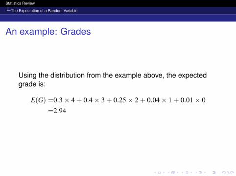
An example: Grades

Using the distribution from the example above, the expectedgrade is:

E(G) =0.3× 4 + 0.4× 3 + 0.25× 2 + 0.04× 1 + 0.01× 0

=2.94

Statistics Review


Interpretation of Expectation as Bet

One interpretation of an expectation is the value of a bet. Iwould break even if the expected value of the bet was zero.

Statistics Review


Example 1: Coin Flip

I get

{$1.00 if heads−$1.00 if tails

Expected payoff is

0.5× 1 + 0.5×−1 = 0.

Statistics Review


Example 2: Die Roll

Suppose you meet a guy on the street who charges you $3.50to play a game. He rolls a die and gives you that amount indollars, i.e. if he rolls a 1 you get $1.00, etc. Is this a good bet?

The expected payoff from the bet is

E (Y − 3.5) =16

1 +16

2 +16

3 +16

4 +16

5 +16

6− 3.5

= 0

Statistics Review


Example 3: Occupation

Suppose you are choosing between being a doctor or a lawyer.You may choose to go into the profession where the expectedearnings are highest.

Statistics Review


Outliers and the ExpectationOutliers are very influential in expected values. Suppose youare a high school basketball player with a remote chance ofbecoming Lebron James. Your distribution of income might looklike

Y =

$20, 000 1

3

$30, 000 199300

$50, 000, 000 1300

Then E(Y) = $166, 748.

One point made by this example is that the mean or expectedvalue is not always a good representation of the typical value orcentral tendency. The median–the value at or above which halfthe realization fall–is $30,000 in the example and is arguablymore typical or central.

Statistics Review


Estimation of Expected Value

You should have learned that the way we estimate the expectedvalue is to use the sample mean

That is suppose we want to estimate E(X) from a sample ofdata X1,X2, ...,XN

We estimate using

X̄ =1N

N∑i=1

Xi

Statistics Review


Example

Suppose data is (as in Wooldridge Example C.1)City Unemployment Rate1 5.12 6.43 9.24 4.15 7.56 8.37 2.68 3.59 5.810 7.5

Statistics Review


In this case

X̄ =5.1 + 6.4 + 9.2 + 4.1 + 7.5 + 8.3 + 2.6 + 3.5 + 5.8 + 7.5

10=6.0

Statistics Review


A fact about sample meansThere is a particular feature of sample means that we will use alot in our course.

Forget about random variables for now and just think about thealgebra.

Notice that for any variable a,

N∑i=1

a(Xi − X̄) =N∑

i=1

aXi −N∑

i=1

aX̄

= aN

[1N

N∑i=1

Xi

]− NaX̄

= NaX̄ − NaX̄

= 0

Statistics Review


Here is one important example of this

s2 =1

N − 1

N∑i=1

(Xi − X̄)2

=1

N − 1

N∑i=1

(Xi − X̄)[Xi − X̄]

=1

N − 1

N∑i=1

(Xi − X̄)Xi −1

N − 1

N∑i=1

(Xi − X̄)X̄

=1

N − 1

N∑i=1

(Xi − X̄)Xi

Statistics Review

Variance




4 Variance





Statistics Review

Variance

Variance

As a first approximation, as the mean is a measure of centraltendency, the variance is a measure of dispersion.

In deciding to make a bet, which occupation to pursue, or whichstocks to buy, we might care not only about the expected payoff,but also its variability. ‘Variability’ captures some notion of risk.

The variance of a random variable is given by:

Var(X) =E(X − µX)2

=J∑

j=1

(xj − µX)2f (xj)

where µX = E(X).

Statistics Review

Variance

If X is nonstochastic xi = µX for all i, so Var(X) = 0.

Var(aX + b) = E(aX + b− (aµX + b))2

= E(aX − aµX)2

= a2E(X − µX)2

= a2Var(X)

The standard deviation is the square root of the variance.

Statistics Review

Variance

Interpretation of Variance

The higher the variance, the less confident you are aboutwhether the outcome will be near the mean (or expectation).

Suppose you bet on a coin toss. Case 1:

X ={

$1.00 heads−$1.00 tails

E(X) = 1× 12

+ (−1)× 12

= 0

V(X) = (1− 0)2 12

+ (−1− 0)2 12

= 1

Statistics Review

Variance

Case 2, you bet $10,000:

X ={

$10, 000 heads−$10, 000 tails

E(X) = 10, 000× 12

+ (−10, 000)× 12

= 0

V(X) = (10, 000− 0)2 12

+ (−10, 000− 0)2 12

= 100, 000, 000

In considering a bet, an investment in a risky project, a ‘lifechoice’ (education, occupation, marriage, etc.), the variance ofthe ‘payoff’ is likely to be relevant.

Statistics Review

Continuous Random Variables




4 Variance





Statistics Review


Continuous Random VariablesThe probability density function shows, heuristically, the ‘relativeprobability’ of a value. Since the random variable is continuousit can take on an infinite number of values and no exact valuehas non–negligible probability. Instead, there is a probability offalling between two points a and b, which is given by

Pr(a ≤ X ≤ b) = area under the curve between a and b

=∫ b

af (x)dx

Thus we also have:

f (x) = limδ→0

Pr(x ≤ X ≤ x + δ)δ

The particular value of the density is not interesting in its ownright. It is only interesting if you integrate over it.

−4 −2 0 2 4

0.0

0.1

0.2

0.3

0.4

x

dnor

m(x

)

An example of a continuous pdf: The normal density function

Statistics Review


Analogous to the properties of the pdf in the discrete case, wehave: ∫

f (x)dx = 1

E(X) =∫

xf (x)dx

Var(X) =∫

(x− E(x))2f (x)dx,

and the properties of expectations that we discussed for thediscrete case carry over.

Statistics Review


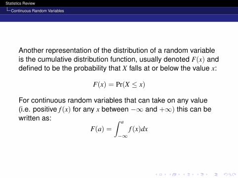
Another representation of the distribution of a random variableis the cumulative distribution function, usually denoted F(x) anddefined to be the probability that X falls at or below the value x:

F(x) = Pr(X ≤ x)

For continuous random variables that can take on any value(i.e. positive f (x) for any x between −∞ and +∞) this can bewritten as:

F(a) =∫ a

−∞f (x)dx

Statistics Review


Joint Distributions of Random Variables

For two random variables X and Y we can define their jointdistribution. For discrete random variables

f (x, y) = Pr(X = x,Y = y)

For continuous random variables:

Pr(a1 ≤ X ≤ a2, b1 ≤ Y ≤ b2) =∫ a2

a1

∫ b2

b1

f (x, y)dydx

Statistics Review

Covariance and Correlation




4 Variance





Statistics Review



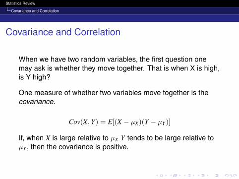
When we have two random variables, the first question onemay ask is whether they move together. That is when X is high,is Y high?

One measure of whether two variables move together is thecovariance.

Cov(X,Y) = E[(X − µX)(Y − µY)]

If, when X is large relative to µX Y tends to be large relative toµY , then the covariance is positive.

Statistics Review


Properties of covariance:

Var(X + Y) = Var(X) + Var(Y) + 2 Cov(X,Y)

Cov(X,X) = Var(X)

Cov(a1X + b1, a2Y + b2) = a1a2Cov(X,Y)

This last property means that if we change the units ofmeasurement of X and/or Y, the covariance changes.

Statistics Review


A measure of association that is ‘unit–free’ is the correlationcoefficient:

ρ(X,Y) =Cov(X,Y)√

Var(X)√

Var(Y)

It turns out that ρ is between −1 and 1. When X and Y areindependent, so there is ‘no relation’ between X and Y, ρ iszero; if ρ > 0 then X and Y go up and down together, whereas ifρ < 0 then when X goes up, Y tends to go down and vice versa.

Statistics Review


Examples of Correlation

Positively correlated random variables:

Years of school, earningsHusband’s wage, wife’s wageStock price, profit of firmGDP, country size

Statistics Review


Negatively correlated random variables:

GDP growth, unemploymentHusband’s income, wife’s hours worked

Statistics Review


Random variables with zero or near–zero correlation

Number on first die, number on second dieMichelle Obama’s temperature, Number of questionsasked in this class todayStock gain today, stock gain tomorrow

Statistics Review


Correlation versus Causality

The difference between causation and correlation is a keyconcept in econometrics. We would like to identify causaleffects and estimate their magnitude. It is generally agreed thatthis is very difficult to do; often a causal interpretation can begiven that is consistent with results derived from an appropriatestatistical procedure; having an economic model is oftenessential in establishing the causal interpretation.

These issues are confused all the time by politicians and thepopular press

For some first thoughts, suppose X and Y are positivelycorrelated.

Statistics Review


Case 1: X → Y (or Y → X)

Money supply→ InflationIncrease in minimum wage→ Increase in wagesRetirement→ Decline in income

Statistics Review


Case 2: X → Y and Y → X

Prices, quantitiesEarnings, hours worked

Statistics Review


Case 3: Z → X and Z → Y

Earnings of wife, earnings of husbandEducation, earningsGDP growth, unemployment

Statistics Review

Normal Random Variables




4 Variance





Statistics Review


Normal Random VariablesNormal random variables play a big role in econometrics–partlybecause they are tractable, partly because normality is arecurring phenomenon in estimation theory.

The distribution of a normal random variable depends only onits mean and variance, i.e. its first two moments. To say itagain, if it’s normal, and you know its mean, and you know itsvariance, you know everything about it. You know its exactdistribution.

The sum of normal random variables is normal.Many distributions (we encounter) are approximatelynormal.

The foregoing facts and what we already know about mean andvariances are important for all that we do.

We will use the notation X ∼ N(µ, σ2) to mean “Randomvariable X is normally distributed with mean µ and variance σ2”

Statistics Review


An Example of Calculations with Normal RandomVariables

SupposeY = a1X1 + a2X2 + c,

where X1 ∼ N(µ1, σ21) and X2 ∼ N(µ2, σ

22), and the covariance

between X1 and X2 is σ12.

What is the distribution of Y?

Statistics Review


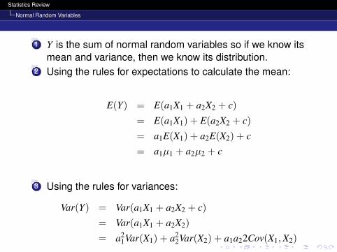
1 Y is the sum of normal random variables so if we know itsmean and variance, then we know its distribution.

2 Using the rules for expectations to calculate the mean:

E(Y) = E(a1X1 + a2X2 + c)= E(a1X1) + E(a2X2 + c)= a1E(X1) + a2E(X2) + c

= a1µ1 + a2µ2 + c

3 Using the rules for variances:

Var(Y) = Var(a1X1 + a2X2 + c)= Var(a1X1 + a2X2)= a2

1Var(X1) + a22Var(X2) + a1a22Cov(X1,X2)

Statistics Review


Therefore we know that:

Y ∼ N(µY , σ2Y)

where

µY = a1µ1 + a2µ2 + c

σ2Y = a2

1Var(X1) + a22Var(X2) + a1a22Cov(X1,X2)

= a21σ

21 + a2

2σ22 + 2a1a2σ12

Statistics Review

Conditional Expectations




4 Variance





Statistics Review



Often the goal of empirical research in economics is to uncoverconditional expectations.

Formally, I could derive the conditional probability densityfunction and derive conditional expectation from that. If you areinterested you can find this in Appendix B of Wooldridge.

Instead I want to think of a conditional expectation in a looserand informal way

The question we often care about is if I could gather everyonein the world for whom X is some particular value, what would bethe expected value of Y

Statistics Review


We define conditional expectation

E (Y | X)

to mean: if I “condition” X to be some value, what is theexpected value of Y?”

In almost all interesting cases

Y is a random variable so after choosing X we don’t knowexactly what Y will beE(Y | X) depends on X, so changing X will change theexpected value of Y

Very often in Economics we care about conditionalexpectations.

Statistics Review


Examples

Lets consider some examples.

Note that all of this fits in the “descriptive” type of analysis weconsider

We are not saying anything about causation

Statistics Review


Wages and GenderLet X be the gender of an individual, we may be very interestedin how wages vary with gender

That is we are interested in

E(wage | male)E(wage | female)

How do we estimate this?

Here it is pretty clear. To estimate an expectation we use themean, to estimate the conditional expectation we use theconditional mean

That is, just take the mean value of wages for men and themean value of wages for women

Statistics Review


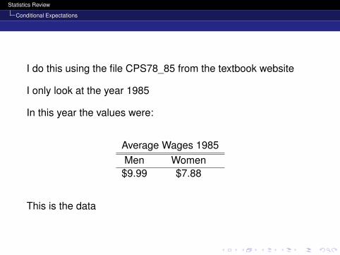
I do this using the file CPS78_85 from the textbook website

I only look at the year 1985

In this year the values were:

Average Wages 1985Men Women

$9.99 $7.88

This is the data

Statistics Review


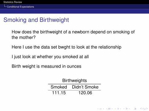
Smoking and Birthweight

How does the birthweight of a newborn depend on smoking ofthe mother?

Here I use the data set bwght to look at the relationship

I just look at whether you smoked at all

Birth weight is measured in ounces

BirthweightsSmoked Didn’t Smoke111.15 120.06

Statistics Review


Baseball Position and Salaries

How do the salaries of baseball players vary with the positionthat they play?

Baseball Salaries

Position SalaryFirst Base $1,586,781

Second Base $1,309,641Third Base $1,382,647Shortstop $1,069,21Catcher $892,519

Outfielder $1,539,324

Statistics Review


Voting Outcomes and Campaign ExpendituresHow does the fraction of votes you get depend on campaignexpenditure?

The raw data looks like this

Statistics Review


How do I estimate this?

Clearly I can’t just condition on all levels of expenditure andtake the mean

We need a model to help us think about this

Documents

Spring Semester, 2011 - SSCC - Homectaber/410/statrev.pdf · 2011-01-14 · Spring Semester, 2011. Statistics Review Outline 1 Random Variables 2 Distribution Functions 3 The Expectation