MARINE ECOLOGY PROGRESS SERIESMar Ecol Prog Ser

Vol. 568: 203–215, 2017https://doi.org/10.3354/meps12082

Published March 24

INTRODUCTION

The phenology of plants and animals is governedby seasonal abiotic events causing predictable changesin favorable conditions for reproduction and growth(Visser & Both 2005, Forrest & Miller-Rushing 2010).In marine ecosystems, important phenological events,such as the spring bloom or the seasonal reproduc-tion in key species, propagate through the food web

with widespread consequences for ecosystem func-tioning. The seasonal advance and retreat of sea icemake the environmental fluctuations in polar seasparticularly strong, causing extreme seasonal varia-tions in physical conditions (Brierley & Thomas 2002,Moline et al. 2008, Ji et al. 2013). In winter, the seaice around Antarctica extends to cover almost 20 mil-lion km2, and is one of the largest and most dynamicecosystems on Earth (Brierley & Thomas 2002). The

© The authors 2017. Open Access under Creative Commons byAttribution Licence. Use, distribution and reproduction are un -restricted. Authors and original publication must be credited.

Publisher: Inter-Research · www.int-res.com

*Corresponding author: per.fauchald@nina.no

Spring phenology shapes the spatial foragingbehavior of Antarctic petrels

Per Fauchald1,*, Arnaud Tarroux2, Torkild Tveraa1, Yves Cherel3, Yan Ropert-Coudert3, Akiko Kato3,4, Oliver P. Love5, Øystein Varpe6,7, Sébastien Descamps2

1Norwegian Institute for Nature Research, Fram Centre, 9296 Tromsø, Norway2Norwegian Polar Institute, Fram Centre, 9296 Tromsø, Norway

3Centres d’Etudes Biologiques de Chizé, UMR7372 du CNRS−Université de La Rochelle, 79360 Villiers-en-Bois, France4Institut Pluridisciplinaire Hubert Curien, CNRS UMR7178, 67037 Strasbourg, France

5Department of Biological Sciences, University of Windsor, Windsor, ON N9B 3P4, Canada6The University Centre in Svalbard, 9171 Longyearbyen, Norway

7Akvaplan-niva, Fram Centre, 9296 Tromsø, Norway

ABSTRACT: In polar seas, the seasonal melting of ice triggers the development of an open-waterecosystem characterized by short-lived algal blooms, the grazing and development of zooplank-ton, and the influx of avian and mammalian predators. Spatial heterogeneity in the timing of icemelt generates temporal variability in the development of these events across the habitat, offeringa natural framework to assess how foraging marine predators respond to the spring phenology.We combined 4 yr of tracking data of Antarctic petrels Thalassoica antarctica with synopticremote-sensing data on sea ice and chlorophyll a to test how the development of melting ice andprimary production drive Antarctic petrel foraging. Cross-correlation analyses of first-passagetime revealed that Antarctic petrels utilized foraging areas with a spatial scale of 300 km. Theseareas changed position or disappeared within 10 to 30 d and showed no spatial consistency amongyears. Generalized additive model (GAM) analyses suggested that the presence of foraging areaswas related to the time since ice melt. Antarctic petrels concentrated their search effort in meltingareas and in areas that had reached an age of 50 to 60 d from the date of ice melt. We found nosignificant relationship between search effort and chlorophyll a concentration. We suggest thatthese foraging patterns were related to the vertical distribution and profitability of the main prey,the Antarctic krill Euphausia superba. Our study demonstrates that the annual ice melt in theSouthern Ocean shapes the development of a highly patchy and elusive food web, underscoringthe importance of flexible foraging strategies among top predators.

KEY WORDS: Area-restricted search · Euphausia superba · Marginal ice zone · Phytoplanktonbiomass · Procellariiformes · Sea ice dynamics · Southern Ocean · Thalassoica antarctica

OPENPEN ACCESSCCESS

Mar Ecol Prog Ser 568: 203–215, 2017

ice pack is the substrate for ice algae, bacteria, andgrazing zooplankton, and is also an important nurs-ery habitat for Antarctic krill Euphausia superba (here -inafter: krill), offering protection from air-breathingsurface predators (Brierley et al. 2002). By seeding,fertilizing, and stabilizing the surface water, the icemelt in spring initiates the characteristically short-lived and patchy phytoplankton blooms (Smith &Nelson 1985, Mitchell & Holm-Hansen 1991, Brierley& Thomas 2002). Spring blooms are an importantfood source for krill, and swarms of feeding krill aretargets for a large number of predators, includingseabirds, pinnipeds, and cetaceans (Fraser & Hof-mann 2003, Smetacek & Nicol 2005, Murphy et al.2007). Much of the distribution range of krill is cov-ered by seasonal or permanent ice, and the timingand intensity of their reproduction is significantlyaffected by the amount of sea ice and the timing ofice retreat (Quetin & Ross 2001, Atkinson et al. 2004,Kawaguchi et al. 2007). Predation pressure on krillfrom air-breathing predators intensifies during sum-mer, possibly forcing the krill to deeper water andde coupling them from their phytoplankton food source(Ainley et al. 2015). Hereinafter, we term the timingof the sequence of ecosystem events initiated by themelting of sea ice the spring phenology. The vast icesheet around Antarctica does not melt synchronously.Thus at a given date in spring, different areas willhave reached different stages in spring phenology.For example, some areas may be in the growth phase,some areas may be at the peak, while others could bein the diminishing phase of the phytoplankton bloom.To predators, the different phenological stages arelikely to offer different levels of availability and prof-itability of prey items. The spatial development of icemelt will accordingly reflect a heterogeneous andtransient distribution of favorable foraging areas, andmobile predators are expected to respond to this het-erogeneity by modifying their habitat utilization andsearch pattern for food.

In this study, we test the prediction that the foragingactivity of Antarctic petrels Thalassoica antarctica inthe Weddell Sea is related to the spring phenology. Inspring and summer, Antarctic petrels forage over vastice-filled or previously ice-filled areas, conducting hierarchical searches (Fauchald 1999) in a patchy,scale-dependent, and transient prey field (Fauchald &Tveraa 2006). We hypothesize that Antarctic petrelsincrease their foraging effort in areas characterized bya favorable phenological stage. Accordingly, as theseason progresses, we would expect Antarctic petrelsto change foraging areas to keep the phenologicalstage of their habitat in a phase that maximizes access

to profitable prey. Krill is a dominant prey item forAntarctic petrels during the breeding season (Lorentsenet al. 1998), and as a surface-feeding predator, we ex-pect the Antarctic petrel to be especially sensitive tochanges in the vertical distribution of krill. Becausewe expect krill to descend to deeper waters as theseason progresses (Ainley et al. 2015), we would ex -pect Antarctic petrels to increase their search effort inareas at an early phenological stage, i.e. around theice melt. To examine this hypothesis, we used remote-sensing data to investigate the spatial pattern of icemelt and the subsequent phenological developmentof surface chlorophyll a (chl a). We used tracking datato examine the foraging patterns of Antarctic petrels,the predictability of their foraging areas, and howtheir foraging effort was related to surface chl a con-centration and time elapsed since ice melt.

MATERIALS AND METHODS

Antarctic petrels

The eastern Weddell Sea is the foraging area ofAntarctic petrels Thalassoica antarctica breeding atSvarthamaren (71° 53’ S, 5° 10’ E) (Lorentsen et al. 1998,Fauchald & Tveraa 2006). Svarthamaren is a nunatak(a mountain peak protruding above the ice sheet) sit-uated approximately 200 km inland in Antarctica, andis the largest known colony of Antarctic petrels, host-ing ca. 200 000 breeding pairs (Des camps et al. 2016).The Antarctic petrel lays its egg when the adjacentocean is still heavily covered with sea ice. By hatchingand early chick-guarding time in late January, themassive sea ice sheet has broken up, and foraging oc-curs over mostly open water until early March, whenfledging occurs. Both parents take part in chick-feed-ing, and krill dominate the prey brought back to thechick (Lorentsen et al. 1998).

Argos and GPS tracking of Antarctic petrels

Antarctic petrels were tracked in 4 different yearsusing Argos satellite transmitters (1996−1997 season)and GPS tags (2011−2014; Table 1). To exclude wronglocations, a basic speed filter was applied on alltracks. Locations situated above the Antarctic ice capor ice shelf (i.e. non-foraging habitat) were also ex -cluded (see Fauchald & Tveraa 2006, Tarroux et al.2016 for details). A polar stereographic projectionwith 0° longitude and 70° standard parallel was usedthroughout the study.

204

Fauchald et al.: Antarctic petrels foraging in Southern Ocean

1996−1997 data

From 18 to 20 January, 36 Antarctic petrels wereequipped with satellite platform terminal transmit-ters (PTTs) at their nest. PTTs (PTT100, 20 and 30 g;Micro wave Telemetry) were attached to the back ofthe birds with a harness covered with TeXon paddingduring their last guarding spell. The weight of thedevice carried by each bird represented on average3.2 and 4.7% (20 and 30 g PTTs, respectively) of theiraverage body mass. The weight was accordinglyslightly larger than the 3% rule proposed by Phillipset al. (2003), suggesting that a detrimental effect withrespect to the cost of flight, foraging success, and massgain during the foraging bout could be ex pected(Passos et al. 2010, Vandenabeele et al. 2012). Har-nesses and transmitters were removed from the birdsas they returned to the colony. Eight birds did notreturn to the colony and 6 either lost their transmitterat an early stage or the transmitter failed to give sig-nals (see Fauchald & Tveraa 2006). In the final data-set, only trips with a defined area-restricted search(ARS) were included (see ‘FPT analyses’ below).According to this procedure, 3 trips were removedfrom the sample, and the final filtered dataset com-prised 5436 positions from 55 trips and 22 individualbirds. Using the location error estimates provided byPinaud & Weimerskirch (2005), the average location

error in the dataset was estimated as 14.2 km(Fauchald & Tveraa 2006). Median time interval be -tween successive Argos locations was 99 min (95%interquantiles: 15−426 min).

2011−2014 data

A total of 131 individuals were tagged with minia-turized GPS units (CatTrack 1, Catnip Technologies)during both the brooding and chick-rearing stages.The GPS units, weighing ca. 20 g, were mounted onthe 2 central rectrices using black Tesa tape, and re -moved when the bird returned to the colony. Datawere then downloaded, projected, and speed- filtered in order to exclude aberrant locations (Tar-roux et al. 2016). Four GPS units failed a few hoursafter the birds had left the colony and did not con-tain usable data. The filtered GPS dataset consistedof 132 353 locations from 133 tracks and 127 individ-uals. First-passage time (FPT) calculations indicatedthat ARS was present for all 133 tracks (see ‘FPTanalyses’ below). By testing 3 units at a known loca-tion in the breeding colony, an average locationerror was estimated as 48 m (95% confidence inter-val [CI]: 14− 81 m). Median time interval betweensuccessive GPS locations was 10 min (95% inter -quantiles: 5− 30 min).

205

1996–1997 2011–2012 2012–2013 2013–2014

No. of trips (tagged ind.) 55 (22) 17 (14) 48 (46) 68 (67)Start of trip (date) Mean 1 Feb 9 Jan 24 Jan 24 Dec Median 27 Jan 9 Jan 23 Jan 19 Dec Date range 20 Jan–28 Feb 13 Dec–7 Feb 26 Dec–11 Feb 29 Nov–22 Jan

Trip duration (d) Mean 7.5 9.6 5.7 10.4 Median 6.6 7.8 5.1 10.2 Min.–max. 2–17 2.6–21.4 2–15.2 1.6–27.4

Trip distance (km) Mean 4171 3744 2709 3330 Median 3909 3961 2377 2759 Min.–max. 868–10 809 587–6453 692–7863 368–9480

Max. dist. colony (km) Mean 1047 1253 853 920 Median 1160 1581 760 817 Min.–max. 261–2524 336–1765 340–1931 327–2061

Ice cover (%) Mean 7.9 32.6 14.3 44.3 Median 8 28 13 48 Min.–max. 6–10 13–61 10–29 22–73

FPT radius (km) Mean 91.5 60.7 65.0 50.2 Median 80 56 51 40 Min.–max. 20–220 7.5–222 5–263 5–219

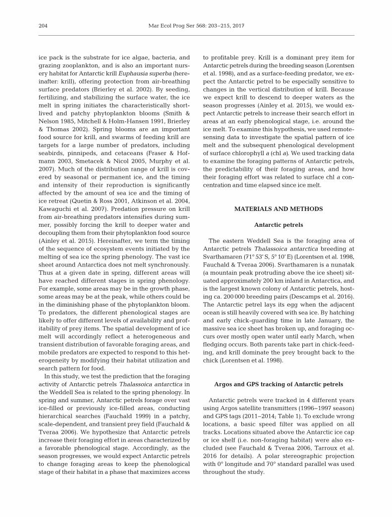
Table 1. Summary statistics of Antarctic petrel Thalassoica antarctica foraging trips during 4 breeding seasons. Number of in-dividuals fitted with PTT tags in 1996–1997 and GPS tags in 2011–2014 are given in parentheses for the number of trips.Mean, median and min.–max. values are shown for other foraging trip characteristics. % ice cover: in the habitat at the start of

the trip. Max. dist. colony: maximum distance from colony; FPT: first-passage time

Mar Ecol Prog Ser 568: 203–215, 2017

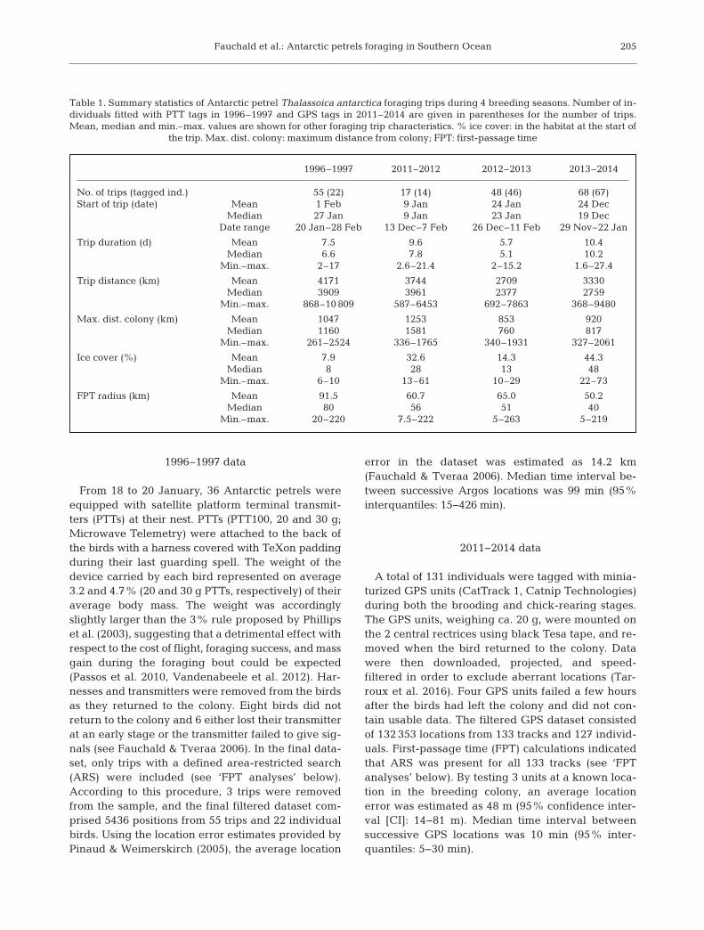
We defined the available foraging habitat as theocean area within a radius of 2000 km from thecolony (Fig. 1), amounting to 7.1 million km2, exclud-ing landmasses and the ice shelf. Percentage icecover in the foraging habitat at the start of each tripvaried between 6 and 73%. In total, the trips covereda distance of >660 000 km, and >99% of the positions

were recorded within areas with either a seasonal ormulti-year ice cover (Fig. 1). Although there was con-siderable overlap, data from different years covereddifferent periods of the breeding season (Table 1).Most notably, 1996−1997 covered the chick-rearingperiod while most of the trips in 2013−2014 tookplace during the brooding period.

Sea ice data and date of ice melt

Data on sea ice concentration were obtained fromthe National Snow and Ice Data Center (http:// nsidc.org/data/NSIDC-0079/versions/2). Measures of seaice concentrations were derived from passive micro-wave measurements from satellites using the dailybootstrap estimates of ice concentration from Nim-bus-7 SMMR and DMSP SSM/I-SSMIS, version 2(Comiso 2000). Ice cover in the study area is at a max-

206

Fig. 1. Study area, foraging trips of Antarctic petrels Thalassoica antarctica (black lines), and seasonal ice habitat in the 4 studyperiods. Light blue: areas with open water throughout the year (maximum ice cover <15%). Grey: area with seasonal ice cover(>15% ice cover on 1 November and open water during summer). White: ice cap or multi-year ice (>50% ice cover on 15March). Black arc (radius = 2000 km from the breeding colony): the defined foraging habitat. Red dot: breeding colony

(Svarthamaren)

Fauchald et al.: Antarctic petrels foraging in Southern Ocean

imum in September and at a minimum in March. Seaice data were obtained for the period 31 October−15 March, thus covering the period of ice melting.For each of the study periods, data were retrieved foreach cell in a 25 × 25 km2 grid covering the Antarcticpetrel’s foraging habitat.

For each grid cell, the date of ice melt was definedby following the ice development forward from31 October and backward from 15 March (see e.g.Stammerjohn et al. 2008 for a similar procedure). Theforward date of ice melt was defined as the first oc -currence of a 7 d running mean ice concentration of<50%. Similarly, the backward date of ice melt wasdefined as the last occurrence of a 7 d running meanice concentration of >50%. In 90% of the cases, theforward and backward dates of ice melt coincided,indicating a relatively rapid diminishing of the icecover with a distinct date of ice melt. In cases wherethe time period between the forward and backwarddates of ice melt was <30 d, the midpoint was used asthe defined date of ice melt. Otherwise, the date ofice melt was defined as unknown.

Chlorophyll data

Daily chl a concentration data (mg m−3) for the years2011−2014 were obtained from the SeaWiFS datasethosted by NOAA’s CoastWatch Program and NASA’sGoddard Space Flight Center, OceanColor Web(http:// oceancolor.gsfc.nasa.gov; O’Reilly et al. 1998).Chl a data were unavailable for the 1996−1997 sea-son. Although cloud cover was generally heavy in thestudy area, limiting the datasets for each year, valuesof chl a were assigned to 32% of the bird positions inthe 3 study periods when chl a data were available,amounting to a total of 78 758 km of tracks. Chl a datacould therefore be used to (1) give a general pictureof the spring bloom phenology in the defined habitatin relation to the time since ice melt, and (2) investi-gate the foraging response of Antarctic petrels tovariation in concentration of chl a in the 2011− 2012,2012−2013, and 2013−2014 seasons.

FPT analyses

FPT (first-passage time) is defined as the time re -quired for an animal to cross a circle of a given radius(r) and can be used to measure the scale-dependentsearch effort along a foraging track (Fauchald &Tveraa 2003, Bailey & Thompson 2006, Freitas et al.2008, Pinaud 2008, Iversen et al. 2014). Each foraging

trip was analyzed separately. To ensure that pointsalong the tracks were equally represented (Pinaud2008), locations were interpolated to obtain a uniformdistance interval of 2 km (Fauchald & Tveraa 2006,Hamer et al. 2009). Based on the interpolated loca-tions, the variance in log-transformed FPT was calcu-lated for r ranging from 2 to 300 km. The r giving themaximum variance in log FPT has been termed theARS scale (Pinaud & Weimerskirch 2005), and corre-sponds to the spatial scale at which the animal con-centrates its search effort. It is also the scale that bestdifferentiates between high and low FPT along thepath (Fauchald & Tveraa 2006). A maximum variancewas undefined in 3 of the 191 tracks (1.6%), i.e. thevariance in log FPT decreased continuously through-out the range of r, suggesting that these birds per-formed an indistinctive ARS or did not use ARS intheir search. These trips were therefore ex cludedfrom the sample (see also Fauchald & Tveraa 2006).For the remaining 188 trips, FPT values were calcu-lated for each interpolated point along the track usingthe r equal to the trip-specific observed ARS scale.

Spatial predictability of foraging areas

To investigate whether the variation in individualFPT values reflected common foraging grounds, andfurthermore, to measure the spatial scale, the dura-tion, and the year-to-year predictability of such areas,spatial and temporal correlograms of the standard-ized FPT values among trips were computed (seeFauchald & Tveraa 2006). First, FPT values from eachtrip were aggregated successively along the paths ona 50 × 50 km2 grid. For each trip, the log10 of the ag -gregated FPT values were Z-scored (mean: 0, SD: 1).Pearson’s correlation coefficients were calculated forall possible pairs of the standardized FPT valuesamong different trips within given distances and timeintervals. For spatial cross-correlograms, time inter-val was kept constant and within ±2 d. For temporalcross-correlograms, distance interval was kept con-stant and equal to 0−100 km. Cross-correlogramswere calculated within and among breeding seasons.Days since 31 October was used to calculate the sea-sonal lags among years.

The 95% CIs for cross-correlation coefficients werecalculated by a delete-one jackknife procedure(Efron & Tibshirani 1993) using trip as the independ-ent statistical unit. Accordingly, the jackknife stan-dard error was calculated on cross-correlation coeffi-cients where 1 trip was left out of the sample at a time(see Fauchald & Tveraa 2006).

207

Mar Ecol Prog Ser 568: 203–215, 2017

Foraging effort and habitat characteristics

Generalized additive models (GAMs) were usedto analyze how the foraging pattern of Antarcticpetrels in terms of FPT changed in response to thestage in spring phenology as indicated by the timesince ice melt and the concentration of chl a. Partlybecause chl a data were only available for 3 of the 4study periods and partly because there was a rela-tively close relationship between the ice melt pat-tern and chl a values (see ‘Results’), analyses weredone separately for the 2 predictor variables. To in -vestigate how the search effort changed as newstages of phenology became available during thecourse of the season, the percentage of ice presentin the available foraging habitat at the start of eachtrip was included as an interaction term in theanalyses.

The dataset used in the analysis of response to phe-nology was compiled by identifying the grid cell fromthe ice data that overlapped with the correspondinginterpolated FPT points, and calculating the time sinceice melt (see ‘Sea ice data and date of ice melt’ above).The resulting dataset comprised 176 trips from 4 studyperiods covering a total length of 513 076 km. For thechl a analyses, all data on chl a within ±5 d and 0−100 km from the FPT point were assigned by interpo-lated distance weighing (IDW). Chl a data were miss-ing in areas with continuous ice and areas with cloudcover, reducing the sample to 32% of the originalbird positions. However, the dataset used in analysesof chl a still comprised 107 trips from 3 study periodsand covering a total length of 78 758 km.

To reduce spatial dependencies in the responsevariable, FPT values from each trip were aggregatedon pre-defined intervals of the predictor variable.Thus, 1 observation in the dataset represented theaverage response in FPT during a trip for a giveninterval in the predictor variable. For the analyses ofthe response to spring phenology, FPT values foreach trip were averaged on 1 d intervals in time sinceice melt. For chl a analyses, FPT values for each tripwere averaged on 0.1 intervals in the log10-trans-formed values of chl a. Finally, to remove systematicdifferences in FPT values among trips in the datasets,the log10-transformed FPT values were Z-scored foreach trip. The dataset on time since ice melt com-prised 2634 observations from 176 trips, with mediannumber of observations (levels of predictors) per tripequal to 15 (min.: 1, max.: 28). The dataset on chl acomprised 2941 observations from 107 trips, withmedian number of observations (levels of predictors)per trip equal to 26 (min.: 3, max.: 55).

We expected non-linear foraging responses to chl aand time since ice melt, and the FPT values wereaccordingly fitted to GAMs using the mgcv library(Wood 2006) in R 3.2.2 (R Development Core Team2016). Moreover, we expected the responses to changeduring the course of the season, and we thereforeincluded percentage ice cover in the foraging habitatat the start of the trip as an interaction term. This wasdone by modeling the predictor as a 2-dimensionalsmooth function where the predictor variable (timesince ice melt or chl a) was combined with percent-age ice cover in the habitat. A thin-plate regressionspline was used as the basis, and the optimal degreeof smoothing was defined by generalized cross-vali-dation (GCV).

Confidence intervals for the response were calcu-lated by a bootstrap procedure using trip as the inde-pendent statistical unit. For each analysis, 10 000bootstrap samples were drawn from the sample offoraging trips (176 and 107 trips for the phenologyand chl a analyses, respectively). GAM analysis wasconducted on each bootstrap sample, and the pre-dicted value for each level of the predictors were cal-culated using the predict function in mgcv. Finally,from the predicted bootstrap values, we calculatedthe mean and 95% CI for the response.

RESULTS

Seasonal changes in habitat characteristics

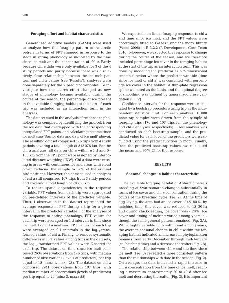
The available foraging habitat of Antarctic petrelsbreeding at Svarthamaren changed substantially interms of ice cover and chl a concentration during thecourse of the breeding cycle (Fig. 2). At the time ofegg-laying, the area had an ice cover of 45−80%; byhatching time, this cover was reduced to 15−30%;and during chick-feeding, ice cover was <20%. Icecover and timing of melting varied among years, al -though the same general pattern re mained (Fig. 2A).While highly variable both within and among years,the average seasonal change in chl a within the for-aging habitat indicated an in crease in phytoplanktonbiomass from early December through mid-January(ca. hatching time) and a decrease thereafter (Fig. 2B).

The relationship between chl a and the time sinceice melt (Fig. 3) revealed a more consistent patternthan the relationships with date in the season (Fig. 2).On average, the data indicated a rapid increase inchl a concentration from the time of ice melt, reach-ing a maximum approximately 20 to 40 d after icemelt and decreasing thereafter (Fig. 3). It is important

208

Fauchald et al.: Antarctic petrels foraging in Southern Ocean

to note that this pattern reflects the average patternin cloud-free open waters, and does not necessarilyreflect the development of individual blooms in theparticular foraging areas used.

Within the foraging habitat, the date of ice meltvaried from 6 November to 15 February (Fig. 4). Gen-erally, ice melt was later the further south. However,the pattern of ice melt was highly variable bothwithin and among years (Fig. 4), suggesting a spatialheterogeneity in the stages of spring phenologyavailable to foraging Antarctic petrels.

ARS and spatial predictability of foraging areas

The cross-correlation in FPT among trips for dis-tances <50 km and time lags <2 d was significantlypositive (Pearson’s correlation coefficient = 0.31, 95%CI: 0.21−0.40) (Fig. 5). Correlations were signifi-cantly positive for distances <300 km, suggestingthat Antarctic petrels increased their foraging effortin overlapping areas at a scale of ~300 km (Fig. 5A).This pattern was absent when computing the cross-correlogram among seasons (Fig. 5C), suggestingthat the foraging areas were not spatially consistentamong the breeding seasons.

Correlations between FPT among trips within thesame area (distance <100 km) decreased with in -creasing time lag, suggesting that foraging areaswere transient also within the season (Fig. 5B). Pear-son’s correlation coefficient leveled off at a value ofapproximately 0.1, with a confidence interval over-lapping zero, after 10 d. Again, the correlations amongdifferent seasons were close to zero (Fig. 5D), inde-pendent of differences between dates, suggesting lit-tle predictability in foraging areas among breedingseasons.

Foraging response to spring phenology

The GAM of the standardized FPT as a function oftime since ice melt and percentage ice cover in thehabitat by the start of the trip showed a relatively low(adjusted R2 = 0.085, n = 2634) and complex (esti-mated degrees of freedom [edf] = 22.2) fit. The re -sponse with respect to time since ice melt for high(50%), medium (30%), and low (10%) ice cover inthe habitat is shown in Fig. 6. Bootstrap analysis(Fig. 6) suggested a significant response under heavyice cover early in the season (Fig. 6A) and under lowice cover late in the season (Fig. 6C), while theresponse was weak in the transitional period with

209

0

0.1

0.2

0.3

0.4

0.5

0.6

0.7

log

chl a

con

cent

ratio

n (m

g m

–3)

2011/12

2012/13

2013/14

0

10

20

30

40

50

60

70

80

90

100

% Ic

e co

ver 1996/97

2011/12

2012/13

2013/14

Egg-laying Fledging

A

Hatching

B

1-Nov 21-Nov 11-Dec 31-Dec 20-Jan 9-Feb 1-Mar 21 Mar

1-Nov 21-Nov 11-Dec 31-Dec 20-Jan 9-Feb 1-Mar 21-Mar

Fig. 2. Seasonal development of (A) percentage ice cover and(B) average chl a concentration (5 d running mean) in theavailable foraging habitat for Antarctic petrels Thalassoicaantarctica breeding in the colony of Svarthamaren. Greybars: approximate timing of major breeding events. Chl a data

were not available for the 1996−1997 season

log

chl a

con

cent

ratio

n (m

g m

–3)

0

0.1

0.2

0.3

0.4

0.5

0.6

0.7

–60 –40 –20 0 60 80 100 12020 40Days since ice melt

2011/12

2012/13

2013/14

Fig. 3. Relationship between average chl a concentrationand time since ice melt in the available foraging habitat forAntarctic petrels Thalassoica antarctica breeding in thecolony of Svarthamaren. Chl a values were averaged overdays since ice melt, irrespective of the date in the season.Chl a data were not available for the 1996−1997 season

Mar Ecol Prog Ser 568: 203–215, 2017

medium ice cover (Fig. 6B). This was confirmed byseparate GAM analyses with respect to time since icemelt for early (ice cover >40%), transitional (icecover between 12 and 40%), and late trips (ice cover<12%). For early trips, the model yielded: adjustedR2 = 0.20, n = 558, edf = 5.1; for the transitional trips:adjusted R2 = 0.04, n = 1152, edf = 6.8; and for long(maximum distance to colony >885 km) and latetrips: adjusted R2 = 0.13, n = 712, edf = 7.6. The model(Fig. 6) suggested that, throughout the season, Ant -arctic petrels in creased their search effort in meltingareas, i.e. areas within ±10 d of the defined date ofice melt. Thus, independent of the ice cover in thehabitat, Antarctic petrels seemed to prefer areaswhere ice was actively melting. However, late in theseason when the ice cover had diminished, and laterphenological stages became available, Antarcticpetrels also increased their effort in areas that hadbeen ice-free for about 50 to 60 d (Fig. 6C).

Foraging relationships with chl a concentrations

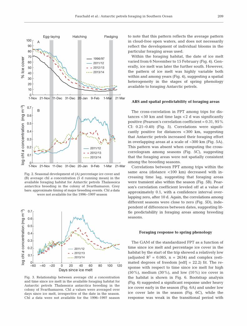
The GAM of the standardized FPT as a function ofchl a concentration and percentage ice cover in thehabitat by the start of each trip showed a low andcomplex fit (adjusted R2 = 0.02, n = 2941, edf = 22.1).Bootstrap analysis revealed weak and non-signifi-cant responses with respect to chl a throughout theseason, i.e. the bootstrap confidence intervals of thepredicted FPT overlapped for all values of chl a(Fig. 7), suggesting that Antarctic petrels in generalwere non-responsive to variation in the surface con-centration of chl a.

DISCUSSION

Ice melt triggers the development of the Antarcticspring and summer open-water ecosystem, including

210

Fig. 4. Spatial pattern in date of ice melt within Antarctic petrel Thalassoica antarctica foraging habitat in the 4 study periods.Foraging habitat (black arc) is defined as the ocean area within a radius of 2000 km from the breeding colony Svarthamaren(red dot). Light blue: areas with open ocean (<15% ice) throughout the study period or areas where the date of ice melt was

undefined (see ‘Materials and methods’). White: ice cap or multi-year ice (>50% ice cover on 1 March)

Fauchald et al.: Antarctic petrels foraging in Southern Ocean 211

–0.4

–0.3

–0.2

–0.1

0

0.1

0.2

0.3

0.4

5 10 15 20 25 30 35

–0.3

–0.2

–0.1

0.4

0.3

0.2

0.1

0

–0.4

–0.3

–0.2

–0.1

0

0.1

0.2

0.3

0.4

200 400 600 800 1000

–0.4 –0.4

–0.3

–0.2

–0.1

0.4

0.3

0.2

0.1

0

Time lag (d)

Pea

rson

’s c

orre

latio

n co

effic

ient

(±95

% C

I)

Distance (km)

A B

0

C

0

5 10 15 20 25 30 35200 400 600 800 10000 0

D

Fig. 5. (A,C) Spatial and (B,D) temporal cross-correlograms of standardized first-passage time among foraging trips of Antarc-tic petrels Thalassoica antarctica. (A,B) are cross-correlograms within breeding seasons while (C,D) are among breeding sea-sons. For the spatial cross-correlograms (A,C), maximum lag between dates of observations was set to 2 d. For the temporalcross-correlograms (B,D), maximum distance between observations was set to 100 km. Grey areas: delete-one jackknife 95%

CI with trip as the statistical unit

–3

–2

–1

0

1

2

3

–40 –20 0 20 40 60 80–40 –20 0 20 40 60 80

–40 –20 0 20 40 60 80–3

–2

–1

–2

–3

3

2

1

0

–1

0

1

2

3

Days since ice melt

Days since ice melt

Firs

t-p

assa

ge t

ime

(Z-s

core

d)

A

B

C

Fig. 6. Standardized first-passage time (FPT) of for-aging Antarctic petrels Thalassoica antarctica as afunction of time elapsed since ice melt at differentseasonal stages of ice retreat (A: 50%, B: 30%, andC: 10% ice cover). Thick lines: mean predicted val-ues ± 95% CIs (shaded areas) from bootstrapped gen-eralized additive models (GAMs) fitting standardizedFPT to a 2-dimensional smoothing of days since icemelt and percentage ice cover in the available habi-tat at the start of the foraging trip. Data points: obser-vations matching the corresponding intervals of per-

centage of ice concentration in the habitat

Mar Ecol Prog Ser 568: 203–215, 2017

a short-lived phytoplankton bloom, the grazing anddevelopment of zooplankton, and the influx of for -aging avian and mammalian predators (Brierley &Thomas 2002, Fraser & Hofmann 2003, Murphy et al.2007). The retreat of the ice is patchy, and at a givendate in spring, different areas have reached differentstages in spring phenology, generating spatial het-erogeneity in the habitat available to top predators.We show that Antarctic petrels responded to this het-erogeneity by concentrating their search effort inmelting areas, i.e. areas within ±10 d from the date ofice melt, showing less interest for areas still heavilycovered with ice and areas that had been ice-free forlonger periods. Late in the season when the ice extentwas at a minimum and older phenological stagesbecame available, birds also selected areas that hadreached an age of 50 to 60 d from the date of ice melt.In other words, the offshore-feeding Antarctic petrelsseemed to prefer areas in specific phenologicalstages determined by the time of ice melt. As a result,their foraging areas changed as the season pro-gressed, reflecting a transient and constantly chang-ing habitat. Remotely sensed measures of chl a indi-cated that the phytoplankton biomass increasedrapidly after the ice melt, reached a maximum after20 to 40 d, and decreased thereafter. This pattern did

not overlap with the phenological stages selectedby the Antarctic petrels, and accordingly, we foundno relationship between the foraging effort of theAntarctic petrels and remotely sensed chl a. In otherwords, areas with high phytoplankton biomass dur-ing the spring bloom maximum were not necessarilyassociated with favorable foraging areas.

The increased foraging effort in areas with meltingice supports the hypothesis that near-surface preypatches were more abundant in areas of an early phe-nological stage. Theory suggests that the vertical dis-tribution of pelagic herbivores is determined by atrade-off between food availability and survival(Ohman 1990, Fiksen et al. 2005), and krill, the domi-nant herbivore of the Antarctic Ocean, is subject tothe same trade-off (Alonzo & Mangel 2001, Cresswellet al. 2009, Ainley et al. 2015). The ice-free surfacelayer is a high-gain, high-risk habitat, while deeperlayers have both lower gain and lower risk (Kaart vedt2010, Ainley et al. 2015). The spring development ofthe open-water ecosystem provides a predictablechange in the abundance of both phyto plankton andmeso-predators, and krill should change their positionin the water column according to the most profitabledepth (Ainley et al. 2015). The predation pressurefrom seabirds, pinnipeds, and cetaceans is expected

212

–4 –3.5 –2.5 –1.5 –0.5 0.5–3 –2 –1 0

–2

–3

–1

0

1

2

3

–4 –3.5 –2.5 –1.5 –0.5 0.5–3 –2 –1 0

–2

–3

–1

0

1

2

3

–4 –3.5 –2.5 –1.5 –0.5 0.5–3 –2 –1 0

–2

–3

–1

0

1

2

3

log10 chl a concentration (mg m–3)

log10 chl a concentration (mg m–3)

Firs

t-p

assa

ge t

ime

(Z-s

core

d)

A

B

C

Fig. 7. Standardized first-passage time (FPT) of for-aging Antarctic petrels Thalassoica antarctica as afunction of remotely sensed chl a concentration atdifferent seasonal stages of ice retreat (A: 50%, B:30%, and C: 10% ice cover). Thick lines: mean pre-dicted values ± 95% CIs (shaded areas) from boot-strapped generalized additive models (GAMs) fittingstandardized FPT to a 2-dimensional smoothing ofchl a and percentage ice cover in the available habi-tat at the start of the foraging trip. Data points: obser-vations matching the corresponding intervals of per-

centage of ice concentration in the habitat

Fauchald et al.: Antarctic petrels foraging in Southern Ocean

to increase as the season develops, suggesting a pro-gressively deeper position of krill (Ainley et al. 2015).Moreover, during the peak phytoplankton bloom, krillmay become unable to convert the excess of high-density food in the surface layer into increasedgrowth (Atkinson et al. 2006), making it more prof-itable to stay below the risky surface habitat. Thesesimple optimality considerations suggest that krillshould be found closest to the surface, and more ac-cessible to surface-feeding seabirds, early in the sea-son before the peak in the spring bloom. This patternhas recently been documented in the Ross Sea (Ainleyet al. 2015), and we suggest that the same mechanismmight be responsible for the increase in search effortamong surface-feeding Antarctic petrels in meltingareas of the Weddell Sea in the present study.

Later in the season, Antarctic petrels also selectedareas that had reached an age of 50 to 60 d since icemelt. We hypothesize that this behavior might reflectthe opportunistic exploitation of a particularly prof-itable life-cycle stage of krill. One such candidate isgravid and spawning krill. Compared to the otherlife-cycle stages of krill, gravid krill are, due to theirhigh lipid content, a highly profitable prey item forchick-rearing seabirds (Chapman et al. 2010). Sev-eral studies have shown that the maturation offemale krill is closely linked to the retreat of the seaice and the subsequent spring bloom (Quetin & Ross2001, Kawaguchi et al. 2007). Because krill need toutilize the algal bloom in order to complete matura-tion (Cuzin-Roudy & Labat 1992), spawning takesplace after the peak in the spring bloom, whichwould coincide with the Antarctic petrels’ selectionof a late phenological stage.

FPT analyses indicated that a large majority of Ant -arctic petrels (188 out of 191 trips) performed ARS.Cross-correlation analyses suggested that the com-mon foraging areas were relatively large with anextent of 300 km, short-lived (with a duration of 10 to30 d), and showed no detectable overlap among years.These characteristics limit the range of environmen-tal factors that possibly could explain the formation ofthe foraging areas. Most importantly, they excludeenvironmental features associated with a fixed spatiallocation such as oceanographic features linked tobathymetry, while pointing towards unstable large-scale features such as the spring bloom and thelarge-scale melting pattern of sea ice. Accordingly,within the Antarctic petrels’ habitat, the date of icemelt ranged from 6 November to 15 February, show-ing a large-scale spatial pattern that differed markedlyamong years (cf. our Fig. 4; see also Massom et al.2013). For Antarctic petrels, the transient and unpre-

dictable nature of the heterogeneity provided by themelting ice, combined with possible interactions withother krill predators, underlines the importance of awide-ranging and flexible foraging strategy. It sug-gests that foragers should respond directly to preypatches (Fauchald 1999) rather than relying on geo-graphically or environmentally fixed foraging habi-tats. In other words, because foraging areas continu-ously change, the birds cannot rely on previous spatialinformation of where to search for food. Foragingdecisions instead are likely based on real-time cuessuch as the observations of other foraging birds(Grünbaum & Veit 2003) or odor cues of e.g. dimethylsulfide released from heavily grazed phytoplankton(Nevitt et al. 1995, 2008).

A system where foragers constantly track movingand unpredictable patches of prey involves a highlystochastic and variable encounter rate, and one couldtherefore expect relatively large variation in theproperties of individual foraging trips (e.g. trip dura-tion, trip length, and ARS scale) and weakly definedforaging areas. Stochastic variation in foraging suc-cess might accordingly be an explanation for thelarge differences found in the ARS scale among trips(5 to 260 km), the relatively weak correlation in for-aging effort among neighboring foraging Antarcticpetrels (cf. Fig. 5), and finally the relatively weak fitof the model explaining foraging effort by phenolog-ical stages (cf. Fig. 6). In fact, the weakly defined andelusive common foraging areas indicated by cross-correlation analyses (Fig. 5) suggest a stochastic sys-tem where little variation could be expected to beexplained by environmental variables. This does notimply that environmental factors are unimportant; itsimply illustrates that the foraging strategy employedby Antarctic petrels produces stochastic noise in therelationships between the factors responsible for theformation of foraging areas and the behavioral re -sponses detected by FPT. In addition to the stochas-ticity in foraging success, it is likely that non-foragingbehavior such as resting might falsely indicate im -portant feeding areas and thereby obscure the rela-tionship between environmental variables and FPT(Sommerfeld et al. 2013). This would be especiallyimportant when the non-foraging activity occurs atspecific locations (e.g. roosting places near the colony)independent of the feeding areas.

Temporal matches (or mis-matches) between foodavailability and predators are important elementsof seasonal environments that heavily influence predator− prey interactions and food web structure(McMeans et al. 2015). In extreme seasonal environ-ments such as the polar seas, mobile predators com-

213

Mar Ecol Prog Ser 568: 203–215, 2017

pensate for temporal variability with spatial flexi -bility. In this context, petrels and albatrosses are suc-cessful since they are exceptionally mobile and searchvery large areas of the ocean’s surface for food. Ourresults suggest that the match between breedingphenology and the onset and development of meltingice, and the subsequent changes in the availabilityand profitability of prey, may be of importance toAntarctic petrels. In particular, we showed that Antarc-tic petrels utilize specific phenological stages, suggest-ing that the availability of these stages during breed-ing could be critical for breeding success. Indeed, forterrestrial herbivores tracking early phenologicalstages of plants during spring, it has been suggestedthat a diversity of altitudinal gradients in the habitatmight be important to ensure a prolonged availabilityof the early and nutritious stages of plants (Mysterudet al. 2001). Similarly, we show that spatial variationin melting ice in the habitat of Antarctic petrels pro-vides a range of phenological stages during thebreeding period. For birds tracking vast areas in thesearch for prey, this diversity is particularly impor-tant, securing the presence of profitable feedinggrounds throughout the breeding cycle. However,contrary to the predictable altitudinal gradients pres-ent in terrestrial habitats, the melting pattern in theSouthern Ocean was relatively unpredictable andoffered few fixed spatial gradients that could aidmobile foragers in tracking profitable phenologicalstages, i.e. ‘moving with the spring’. The spatiallyvariable annual ice melt pattern in the SouthernOcean shapes the development of a highly patchyand elusive food web underscoring the importance offlexible foraging strategies among top predators.

Acknowledgements. This work was supported by the Nor-wegian Antarctic Research Expedition program of the Nor-wegian Research Council (grant no. 2011/70/8/KH/is toS.D.). We are very grateful to our dedicated field assistants(S. Haaland, G. Mabille, T. Nordstad, E. Soininen, and J.Swärd). We thank H. Jensen for help with fieldwork in the1996−97 season. We thank the logistic department at theNorwegian Polar Institute and the Troll Station summer andwintering teams for field support. N. G. Yoccoz gave valu-able comments on earlier drafts.

LITERATURE CITED

Ainley DG, Ballard G, Jones RM, Jongsomjit D, Pierce SD,Smith WO Jr, Veloz S (2015) Trophic cascades in thewestern Ross Sea, Antarctica: revisited. Mar Ecol ProgSer 534: 1−16

Alonzo SH, Mangel M (2001) Survival strategies and growthof krill: avoiding predators in space and time. Mar EcolProg Ser 209: 203−217

Atkinson A, Siegel V, Pakhomov E, Rothery P (2004) Long-term decline in krill stock and increase in salps withinthe Southern Ocean. Nature 432: 100−103

Atkinson A, Shreeve RS, Hirst AG, Rothery P and others(2006) Natural growth rates in Antarctic krill (Euphausiasuperba): II. Predictive models based on food, temperature,body length, sex, and maturity stage. Limnol Oceanogr51: 973−987

Bailey H, Thompson P (2006) Quantitative analysis of bottle-nose dolphin movement patterns and their relationshipwith foraging. J Anim Ecol 75: 456−465

Brierley AS, Thomas DN (2002) Ecology of Southern Oceanpack ice. Adv Mar Biol 43: 171−276

Brierley AS, Fernandes PG, Brandon MA, Armstrong F andothers (2002) Antarctic krill under sea ice: elevatedabundance in a narrow band just south of ice edge. Science 295: 1890−1892

Chapman EW, Hofmann EE, Patterson DL, Fraser WR (2010)The effects of variability in Antarctic krill (Euphausiasuperba) spawning behavior and sex/maturity stage dis-tribution on Adelie penguin (Pygoscelis adeliae) chickgrowth: a modeling study. Deep Sea Res II 57: 543−558

Comiso JC (2000) Bootstrap sea ice concentrations fromNimbus-7 SMMR and DMSP SSM/I-SSMIS, version 2.http://nsidc.org/data/docs/daac/nsidc0079_bootstrap_seaice.gd.html

Cresswell KA, Tarling GA, Thorpe SE, Burrows MT,Wiedenmann J, Mangel M (2009) Diel vertical migrationof Antarctic krill (Euphausia superba) is flexible duringadvection across the Scotia Sea. J Plankton Res 31: 1265−1281

Cuzin-Roudy J, Labat JP (1992) Early summer distribution ofAntarctic krill sexual development in the Scotia-Weddellregion: a multivariate approach. Polar Biol 12: 65−74

Descamps S, Tarroux A, Lorentsen SH, Love OP, Varpe Ø,Yoccoz NG (2016) Large-scale oceanographic fluctua-tions drive Antarctic petrel survival and reproduction.Ecography 39: 496−505

Efron B, Tibshirani RJ (1993) An introduction to the boot-strap. Chapman & Hall/CRC, Boca Raton, FL

Fauchald P (1999) Foraging in a hierarchical patch system.Am Nat 153: 603−613

Fauchald P, Tveraa T (2003) Using first-passage time in theanalysis of area-restricted search and habitat selection.Ecology 84: 282−288

Fauchald P, Tveraa T (2006) Hierarchical patch dynamicsand animal movement pattern. Oecologia 149: 383−395

Fiksen O, Eliassen S, Titelman J, Fiksen Ø (2005) Multiplepredators in the pelagic: modelling behavioural cas-cades. J Anim Ecol 74: 423−429

Forrest J, Miller-Rushing AJ (2010) Toward a syntheticunderstanding of the role of phenology in ecology andevolution. Philos Trans R Soc B 365: 3101−3112

Fraser WR, Hofmann EE (2003) A predator’s perspective oncausal links between climate change, physical forcingand ecosystem response. Mar Ecol Prog Ser 265: 1−15

Freitas C, Kovacs KM, Lydersen C, Ims RA (2008) A novelmethod for quantifying habitat selection and predictinghabitat use. J Appl Ecol 45: 1213−1220

Grünbaum D, Veit RR (2003) Black-browed albatrosses for-aging on Antarctic krill: density-dependence throughlocal enhancement? Ecology 84: 3265−3275

Hamer KC, Humphreys EM, Magalhães MC, Garthe S andothers (2009) Fine-scale foraging behaviour of a medium-ranging marine predator. J Anim Ecol 78: 880−889

214

Fauchald et al.: Antarctic petrels foraging in Southern Ocean

Iversen M, Fauchald P, Langeland K, Ims RA, Yoccoz NG,Bråthen KA (2014) Phenology and cover of plant growthforms predict herbivore habitat selection in a high lati-tude ecosystem. PLOS ONE 9: e100780

Ji R, Jin M, Varpe Ø (2013) Sea ice phenology and timing ofprimary production pulses in the Arctic Ocean. GlobChange Biol 19: 734−741

Kaartvedt S (2010) Diel vertical migration behaviour of thenorthern krill (Meganyctiphanes norvegica Sars). AdvMar Biol 57: 255−275

Kawaguchi S, Yoshida T, Finley L, Cramp P, Nicol S (2007)The krill maturity cycle: a conceptual model of the sea-sonal cycle in Antarctic krill. Polar Biol 30: 689−698

Lorentsen SH, Klages N, Røv N (1998) Diet and prey con-sumption of Antarctic petrels Thalassoica antarctica atSvarthamaren, Dronning Maud Land, and at sea outsidethe colony. Polar Biol 19: 414−420

Massom R, Reid P, Stammerjohn S, Raymond B, Fraser A,Ushio S (2013) Change and variability in east Antarcticsea ice seasonality, 1979/80–2009/10. PLOS ONE 8: e64756

McMeans BC, McCann KS, Humphries M, Rooney N, FiskAT (2015) Food web structure in temporally-forced eco-systems. Trends Ecol Evol 30: 662−672

Mitchell BG, Holm-Hansen O (1991) Observations of model-ing of the Antartic phytoplankton crop in relation to mix-ing depth. Deep Sea Res A 38: 981−1007

Moline MA, Karnovsky NJ, Brown Z, Divoky GJ and others(2008) High latitude changes in ice dynamics and theirimpact on polar marine ecosystems. Ann N Y Acad Sci1134: 267−319

Murphy EJ, Watkins JL, Trathan PN, Reid K and others(2007) Spatial and temporal operation of the Scotia Seaecosystem: a review of large-scale links in a krill centredfood web. Philos Trans R Soc B 362: 113−148

Mysterud A, Langvatn R, Yoccoz NG, Stenseth NC (2001)Plant phenology, migration and geographical variation inbody weight of a large herbivore: the effect of a variabletopography. J Anim Ecol 70: 915−923

Nevitt GA, Veit RR, Kareiva P (1995) Dimethyl sulphide as aforaging cue for Antarctic Procellariiform seabirds. Nature376: 680−682

Nevitt GA, Losekoot M, Weimerskirch H (2008) Evidence forolfactory search in wandering albatross, Diomedea exu-lans. Proc Natl Acad Sci USA 105: 4576−4581

O’Reilly JE, Maritorena S, Mitchell BG, Siegel DA and oth-ers (1998) Ocean color chlorophyll algorithms for Sea-WiFS. J Geophys Res Oceans 103: 24937−24953

Ohman MD (1990) The demographic benefits of diel vertical

migration by zooplankton. Ecol Monogr 60: 257−281Passos C, Navarro J, Giudici A, González-Solís J (2010) Ef -

fects of extra mass on the pelagic behavior of a seabird.Auk 127: 100−107

Phillips RA, Xavier JC, Croxall JP (2003) Effects of satellitetransmitters on albatrosses and petrels. Auk 120: 1082−1090

Pinaud D (2008) Quantifying search effort of moving ani-mals at several spatial scales using first-passage timeanalysis: effect of the structure of environment andtracking systems. J Appl Ecol 45: 91−99

Pinaud D, Weimerskirch H (2005) Scale-dependent habitatuse in a long-ranging central place predator. J Anim Ecol74: 852−863

Quetin LB, Ross RM (2001) Environmental variability and itsimpact on the reproductive cycle of Antarctic krill. AmZool 41: 74−89

R Development Core Team (2016) R: a language for statisti-cal computing. R Foundation for Statistical Computing,Vienna

Smetacek V, Nicol S (2005) Polar ocean ecosystems in achanging world. Nature 437: 362−368

Smith WO, Nelson DM (1985) Phytoplankton bloom pro-duced by a receding ice edge in the Ross Sea: spatialcoherence with the density field. Science 227: 163−166

Sommerfeld J, Kato A, Ropert-Coudert Y, Garthe S, HindellMA (2013) Foraging parameters influencing the detec-tion and interpretation of area-restricted search behav-iour in marine predators: a case study with the maskedbooby. PLOS ONE 8: e63742

Stammerjohn SE, Martinson DG, Smith RC, Iannuzzi RA(2008) Sea ice in the western Antarctic Peninsularegion: spatio-temporal variability from ecological andclimate change perspectives. Deep Sea Res II 55: 2041−2058

Tarroux A, Weimerskirch H, Wang SH, Bromwich DH andothers (2016) Flexible flight response to challengingwind conditions in a commuting Antarctic seabird: Doyou catch the drift? Anim Behav 113: 99−112

Vandenabeele SP, Shepard EL, Grogan A, Wilson RP (2012)When three per cent may not be three per cent; device-equipped seabirds experience variable flight constraints.Mar Biol 159: 1−14

Visser ME, Both C (2005) Shifts in phenology due to globalclimate change: the need for a yardstick. Proc R Soc B272: 2561−2569

Wood SN (2006) Generalized additive models: an introduc-tion with R. Chapman & Hall/CRC, Boca Raton, FL

215

Editorial responsibility: Rory Wilson, Swansea, UK

Submitted: April 19, 2016; Accepted: February 7, 2017Proofs received from author(s): March 10, 2017