Spring Cleaning: Rural Water Impacts,

Valuation and Property Rights Institutions*

Michael Kremer Harvard University,

Brookings Institution, and NBER

Jessica Leino World Bank

Edward Miguel University of California, Berkeley

and NBER

Alix Peterson Zwane

Bill and Melinda Gates Foundation

First draft: July 2006

This draft: August 2009

Abstract: In many societies, social norms create common property rights in natural resources, limiting incentives for private investment. This paper uses a randomized evaluation in Kenya to measure the health impacts of investments to improve source water quality through spring

protection, estimate the value that households place on spring protection, and simulate the welfare impacts of alternative water property rights norms and institutions, including common property, freehold private property, and alternative “Lockean” property rights norms. We find that infrastructure investments reduce fecal contamination by 66% at naturally occurring springs, cutting child diarrhea by one quarter. While households increase their use of protected springs, travel-cost based revealed preference estimates of households’ valuations are only one-half stated preference valuations and are much smaller than levels implied by health planners’ typical valuations of child mortality, consistent with models in which the demand for health is highly income elastic. Simulations suggest that, at current income levels, private property norms would generate little additional investment while imposing large static costs due to spring owners’ local market power, but that private property norms might function better than common property at higher income levels. Alternative institutions, such as “modified Lockean” property rights, government investment or vouchers for improved water, could yield higher social welfare.

* This research is supported by the Hewlett Foundation, USDA/Foreign Agricultural Service, International Child Support, Swedish International Development Agency, Finnish Fund for Local Cooperation in Kenya, google.org, the Bill and Melinda Gates Foundation, and the Sustainability Science Initiative at the Harvard Center for International Development. We thank Alicia Bannon, Jeff Berens, Lorenzo Casaburi, Carmem Domingues, Willa Friedman, Francois Gerard, Anne Healy, Jonas Hjort, Jie Ma, Clair Null, Owen Ozier, Camille Pannu, Changcheng Song, Eric Van Dusen, Melanie Wasserman, and Heidi Williams for excellent research assistance, and thank the field staff, especially Polycarp Waswa and Leonard Bukeke. Jack Colford, Alain de Janvry, Giacomo DiGiorgi, Esther Duflo, Liran Einav, Andrew Foster, Michael Greenstone, Avner Greif, Michael Hanemann, Danson Irungu, Ethan Ligon, Steve Luby, Chuck Manski, Enrico Moretti, Kara Nelson, Aviv Nevo, Sheila Olmstead, Ariel Pakes, Judy Peterson, Pascaline Dupas, Rob Quick, Mark Rosenzweig, Elisabeth Sadoulet, Sandra Spence, Duncan Thomas, Ken Train, Chris Udry, and many seminar participants have provided helpful comments. Opinions presented here are those of the authors and not those of the Bill and Melinda Gates Foundation or its leadership. All errors are our own.

1

1. Introduction

Many view movement toward private property rights institutions as critical to successful economic

development (De Soto, 1989, North, 1990). Yet social norms and formal laws often create communal

property rights in natural resources. In Islamic law, for example, the sale of water is generally not

permitted (Faruqui, Biswas, and Bino 2001), and in societies from Tsarist Russia to contemporary

west and southern Africa, land is periodically reallocated among families based on assessments of

need (e.g., Adams et al. 1999, Bartlett 1990, Fafchamps and Gavian 1996, Peters 2007). Some argue

that communities often develop effective institutions for addressing collective action problems

around common property resource use (Ostrom 1990).

In Kenya, both social norms and law make many water sources, including naturally occurring

springs, common property resources (Mumma 2005). This potentially discourages private

investment in water infrastructure, such as the spring protection technology we examine. Protection

seals off the source of a spring and thus reduces water contamination. On the other hand, communal

property rights in water also limit static inefficiencies due to exploitation of local market power.

This paper makes four principal contributions. First, we provide what to our knowledge is the

only evidence from a randomized impact evaluation on the health benefits of a source water quality

intervention, a significant area of government and donor investment in less developed countries.

Second, we provide among the first revealed preference estimates of the value of child health gains

and a statistical life in a poor country. Our estimates fall far below those typically used by health

economists in assessing cost effectiveness of health policies and suggest that the demand for health is

highly income elastic, as argued by Hall and Jones (2007). Third, we contribute to the literature on

the valuation of environmental amenities, providing evidence on the divergence between revealed

and stated preference valuation for water-related interventions. Finally, we combine data from our

randomized experiment with structural econometric methods used by Berry, Levinsohn, and Pakes

(1995) and others1 to explore the implications of alternative property rights regimes in natural

resources, shedding light on the role of social norms and institutions in economic development

(Acemoglu, Johnson and Robinson 2001).

1 Several recent papers combine data from randomized experiments with structural econometric methods in development economics, the best known probably being Todd and Wolpin (2006), who use experimental estimates from Mexico to validate a structural model of educational investment. We do not seek to validate a particular model in this paper, but rather combine experimental results with a structural model of water infrastructure investment to explore the implications of alternative property rights institutions on social welfare.

2

Policymakers have called for more investment in water infrastructure in less developed

countries to provide cleaner water and reduce water-borne diseases such as diarrhea, which accounts

for 20% of deaths of children under five each year (Bryce et al. 2005). Progress towards the sole

quantifiable environmental Millennium Development Goal is currently measured by the percentage

of population living near improved water sources such as protected springs. Yet there is controversy

about the health value of improvements that fall short of piping treated water into the home. In the

absence of evidence from randomized trials, several influential reviews argue based on non-

experimental evidence that there may be little point in investing in other water infrastructure because

diarrhea is affected more by the quantity of water available for washing than by drinking water

quality (Curtis, Carincross, and Yonli 2000); improved water supply has little impact without good

sanitation and hygiene (Esrey 1996, Esrey et al. 1991); and water recontamination in transport and

storage may dampen some of the benefits of improved source water quality (Fewtrell et al. 2004).

As the first (to our knowledge) randomized evaluation of a source water quality investment,

the data used in this paper allow us to isolate the impact of a single intervention affecting the quality

but not quantity of water, and to assess child health impacts.2 We find that spring protection greatly

improves water quality at the source, reducing fecal contamination by 66%, and is moderately

effective at improving household water quality, reducing contamination 24%. Diarrhea among young

children in treatment households falls by 4.7 percentage points, or nearly one quarter on a base

diarrhea prevalence of approximately 19 percent. The incomplete pass through of spring-level water

gains into the home is due both to households’ collection of water from multiple sources and to

partial recontamination of the water in transport and storage. There is no evidence that spring

protection crowds out household water treatment measures such as boiling or chlorination. There is

also no evidence that improved sanitation coverage or hygiene knowledge allows households to

better translate source water quality gains into larger improvements in household water quality.

The second part of this paper focuses on the valuation of environmental amenities. In our

study area, most households choose from multiple local water sources. The intervention we study

generates exogenous variation in the relative desirability of alternative sources, and we explore how

household water source choices respond to these water quality improvements. A discrete choice

model, in which households trade off water quality against walking distance to the source, generates

2 Two prospective studies of source water quality interventions find positive child health impacts (Aziz et al. 1990, Huttly et al. 1987), but the published articles do not mention if the treatment villages were randomly selected, and generalizing to other settings is hampered by their small sample sizes (five villages each), and they evaluate improved water quality and quantity simultaneously.

3

revealed preference estimates of household valuations of better water quality. Households’ estimated

mean annual valuation for spring protection is equivalent to 32.4 workdays. Based on household

reports on the tradeoffs they face between money and walking time, this corresponds to

approximately US$2.96 per household per year. Under some stronger assumptions this translates to

an upper bound of $0.89 on households’ mean willingness to pay to avert one child diarrhea episode,

and $769 on the mean value of averting one statistical child death, or $23.68 to avert the loss of one

disability-adjusted life year (DALY). These fall far below the values typically used in health cost-

effectiveness analyses in low-income countries, where investments that prevent the loss of one

DALY for less than $100 or $150 are often assumed to be appropriate. These results are consistent

with an income elasticity of demand for health far greater than one.

We contrast the revealed preference valuation of spring protection, which exploits

experimental variation in water source characteristics, with two stated preference methodologies:

stated ranking of alternative water sources, and contingent valuation (Carson et al. 1996, Whitehead

2006). Most valuation estimates rely on such stated preference data, which is relatively cheap to

collect, yet few stated preference estimates have been validated against reliable benchmarks since

revealed preference data is rarely available in less developed countries, and many studies that do

exist are prone to omitted variable bias critiques.3 We find that stated preference approaches generate

much higher valuations than revealed preference estimates, by a factor of two, with contingent

valuation yielding especially imprecise estimates, casting doubt on their reliability in this setting.

Our final set of results simulates the impact of alternative social norms and property rights

institutions in the rural water sector. We first show that a social planner maximizing welfare as

captured by our revealed preference valuation estimates would only protect springs with a relatively

large number of household users, but that a paternalistic social planner who valued health at the

levels typically used by health planners would protect many more springs. Using the household water

demand system derived from the revealed preference valuations, we then conduct counterfactual

simulations and find that alternative property rights institutions have important social welfare

3 Madajewicz et al (2007) find considerable responsiveness to information on water source arsenic contamination in household water source choices in Bangladesh. Whittington, Mu, and Roche (1990) and Mu, Whittington, and Briscoe (1990) each study water source choice in rural Africa using a contingent valuation (CV) approach. However, neither considers water quality in the source choice decision and they explicitly rule out multiple drinking water sources, which we find to be empirically important. Choe (1996) compares willingness to pay for reduced river and lake pollution in an urban Philippines setting with piped water, using both travel cost and CV methods, and finds that both are similarly low but this may not generalize to rural areas. Two other papers have compared averting expenditure data to stated willingness to pay (Griffin et al. 1995 and Rosado et al. 2006 in India and Brazil, respectively), though neither exploits experimental variation in water quality. Diamond and Hausman (1994) discuss the limitations of stated preference approaches to measuring the value of non-market goods.

4

consequences. We first find that a freehold private property rights norm would yield lower social

welfare than existing communal rights because the static losses from spring owners pricing above

marginal cost outweigh the dynamic benefits of greater water infrastructure investment incentives,

providing a rationale for why communal water norms in rural Africa have not generally been

displaced by private property rights. However, we estimate that as demand for clean water rises – for

instance, at higher income levels – private property norms do yield higher social welfare than

common property norms, potentially shedding light on the role that underlying economic conditions

might play in the evolution of social norms and institutions.

We also show that an alternative “modified Lockean” norm under which spring owners can

charge for protected spring water only if they also allow continued free access to unprotected water

generates a Pareto improvement relative to existing communal property norms. Finally, public

investment or a government-financed voucher system for spring users could approximate the solution

for either a social planner who respects households’ spring protection valuations or a paternalistic

planner who places extra value on child health.

The paper is organized as follows. Section 2 describes the intervention and data. Section 3

presents spring protection impacts on water quality and child health. Section 4 discusses the effect of

protection on water source choice and estimates the willingness to pay for spring protection. Section

5 presents social welfare under alternative institutions, and the final section concludes.

2. Rural Water Project (RWP) overview and data

This section describes the intervention, randomization into treatment groups, and data collection.

2. 1 Spring protection in western Kenya

Spring protection is widely used in non-arid regions of Africa to improve water quality at existing

spring sources (Mwami 1995, Lenehan and Martin 1997, UNEP 1998). Protection seals off the

source of a naturally occurring spring and encases it in concrete so that water flows out from a pipe

rather than seeping from the ground, where it is vulnerable to contamination when people dip vessels

into the water to scoop out water and when runoff from the surrounding area introduces human or

animal waste into the area. As spring protection technology has no moving parts, it requires far less

maintenance than other water infrastructure such as pumps.

Naturally occurring springs are an important source of drinking water in rural western Kenya.

Approximately 43% of rural western Kenyan households use springs for drinking water and over

90% have access to springs (DHS 2003). Survey respondents in our study area report that springs are

5

their main source of water: 72% of all water collection trips are to springs. The next most common

source are shallow wells (at 13%), followed by boreholes (7%), and surface water sources such as

rivers, lakes and ponds (5%). Over 81% of all water collection trips in the last week are to sources

the respondents used for drinking water (as opposed to strictly for other household needs).

Most springs in our study area are located on private land. In Kenya, property rights to land

and other natural resources are governed by a combination of traditional customary law and formal

legal statutes (Mumma 2005). Not only does custom require that private landowners allow public

access to water sources on their land, but also under Kenyan law local authorities can “where, in the

opinion of the Authority the public interest would be best served” order water source owners to make

water available “to any applicant so long as the water use of the owner of the works is not adversely

affected.” In practice landowners in our study area are expected to make spring water available to

neighbors for free.4 Spring water simply runs off if not collected. However, this implies that spring

owners have weak incentives to improve water sources, as they are unable to recoup the costs of any

investment via the collection of user fees.

This study is based on a randomized evaluation of a spring protection project conducted by a

non-governmental organization (NGO), International Child Support (ICS). As implemented by ICS,

spring protection included installing fencing and drainage and organizing a user maintenance

committee, in addition to the actual construction. Spring protection cost an average of US$1024 (s.d.

$85), with some variation depending on land characteristics. All communities contributed 10% of

project costs, mainly in the form of manual labor. After construction, the committees undertake

routine maintenance, including simple patching of concrete, cleaning the catchment area, and

clearing drainage ditches. These costs are roughly $35 per year, and are typically expected to be

covered by local contributions, although free rider problems in collecting these funds are common.

2.2 The study sample and assignment to treatment

Springs for this study were selected from the universe of local unprotected springs. The NGO first

obtained Kenya Ministry of Water and Irrigation lists of all local unprotected springs in Busia and

Butere-Mumias districts. NGO technical staff then visited each site to determine which springs were

suitable for protection. Springs known to be seasonally dry were eliminated, as were sites with

upstream contaminants (e.g., latrines, graves). From the remaining suitable springs, 200 were

4 However, in another rural Kenyan region, local officials do sometimes permit landowners to charge for access to spring water once the landowners have invested in spring protection (personal communication with Scott Lee).

6

randomly selected (using a computer random number generator) to receive protection. Permission for

protection was received from the spring landowner in all but two cases.

The NGO planned for the water quality improvement intervention to be phased in over four

years due to their financial and administrative constraints. Although all springs were eventually

protected, for our analysis the springs protected in round 1 (January-April 2005) and round 2

(August-November 2005) are called the treatment springs and those that were protected later are the

comparison group.5 To address concerns about seasonal variation in water quality and disease

burden, all springs were stratified geographically and by treatment group and then randomly assigned

to an activity “wave,” and all project activities and data collection were conducted by wave.

Several springs were unexpectedly found to be unsuitable for protection after the baseline data

collection and randomization had already occurred. These springs, which were found in both the

treatment and comparison groups, were dropped from the sample, leaving 184 viable springs.

Identification of the final sample of viable springs is not related to treatment assignment: when the

NGO was first informed that some springs were seasonally dry, all 200 sample springs were re-

visited to confirm their suitability for protection. In only 10 springs among the final sample of 184

viable springs did treatment assignment differ from actual treatment (for example because

landowners refused to allow protection, or the government independently protected comparison

springs); these springs are retained in the sample and we conduct an intention-to-treat analysis

throughout. Table 1 presents baseline summary statistics for the treatment and comparison groups.6

A representative sample of households that regularly used each sample spring was selected at

baseline. Survey enumerators interviewed users at each spring, asking their names as well as the

names of other household users. Enumerators elicited additional information on spring users from the

three to four households located nearest to the spring. Households that were named at least twice

among all interviewed subjects were designated as “spring users”. The number of household spring

users varied from eight to 59 with a mean of 31. Seven to eight households per spring were randomly

selected from this spring user list for the household sample we use. In subsequent surveys, over 98%

of this sample was found to actually use the spring at least sometimes; the few non-users were

nonetheless retained in the analysis. The spring user list is reasonably representative of all

households living near sample springs. In a census of all households living near nine sample springs

that was conducted near the end of data collection, 71% of households living less than a 20 minute

5 Appendix Figure 1 summarizes the project timeline. 6 Additional details about the randomization into treatment groups are in Supplementary Appendix A.

7

walk from the source were included in the original spring users lists, with even higher rates of

inclusion (77%) for those households less than a 10 minute walk from the spring.

2.3 Data collection

Water quality was measured at all sample springs and households using protocols based on those

used at the U.S. Environmental Protection Agency. The water quality measure we use is

contamination with E. coli, an indicator bacteria that is correlated with the presence of fecal matter.

The household survey gathered baseline information about child diarrhea and anthropometrics,

mothers’ hygiene knowledge and behaviors (hand washing), household water collection and

treatment behavior, and socioeconomic status. The target survey respondent was the mother of the

youngest child living in the home compound (where extended families often co-reside), or another

woman with childcare responsibilities if the mother of the youngest child was unavailable.7

A first follow-up round of water quality testing at the spring and in homes, spring environment

surveys, and household surveys was completed three to four months after the first round of spring

protection (April-August 2005). The second round of spring protection was in August-November

2005, and the second follow-up survey one year later (August-November 2006). The third follow-up

survey round took place five months later, (January-March 2007). The main analysis sample consists

of 184 springs and 1,354 households with baseline data and at least one round of follow-up data.

Attrition was modest: 94% of baseline households were surveyed in at least two of the three

follow-ups and 80% were surveyed in all three follow-up rounds. Attrition is not significantly related

to spring protection assignment: the estimated coefficient on treatment is 0.012 (s.e. 0.018). The

characteristics of households lost over time are statistically indistinguishable from those that remain.

An intervention providing point-of-use (POU), or in-home, chlorination products was launched

before the third follow-up survey (2007) in a random subset of households. Due to possible

interactions with spring protection and impacts on household water quality and health, the third

follow-up survey for this subset of households is excluded from the analysis. This POU intervention

is studied in other research (Kremer, Miguel, Null and Zwane 2008).

2.4 Baseline descriptive statistics

Table 1 presents baseline summary statistics for springs (Panel A), households (Panel B) and children

under age three (Panel C). For completeness, we report statistics for all springs and households with

baseline data (collected prior to randomization into treatment groups) even if they are dropped from

7 Details on the data collection protocols are in Supplementary Appendix B.

8

the analysis because the spring was later found unsuitable for protection, although results are almost

unchanged with the slightly smaller main sample (not shown). As expected with the randomization,

there is no statistically significant difference between baseline water quality at treatment versus

comparison springs (Panel A). Using water quality designations drawn from EPA standards, most

spring water is of moderate quality, only about 5-6% of samples are of high quality, and the rest are

poor quality. Household water is somewhat more likely to be high quality prior to spring protection

in the treatment group (and the difference in means, though small, is significant at 95% confidence),

but there is no significant difference in the proportion of moderate or poor quality water (Panel B). A

Kolmogorov-Smirnov test cannot reject equality of baseline home water quality distributions for the

treatment and comparison groups (p-value=0.24).

Household water quality is somewhat better than spring water quality on average at baseline:

the average difference in ln E. coli is 0.51 (s.d. 2.63; results not shown). This likely occurs for at least

two reasons. First, many households collect water from sources other than the sample spring: only

half of the households get all their drinking water from their spring at baseline, and overall nearly

one third of water collection trips are to other sources. Second, at baseline 25% of households report

that they boiled their drinking water yesterday. However, it is worth noting that even in those

households, both adults and children often drink some unboiled water; for instance, young children

are commonly given water to drink directly from the household storage container. Moreover, the

correlation between household water contamination and self-reported boiling is low, raising the

possibility of social desirability reporting bias. Finally, some households may chlorinate their water.

Following a 2005 cholera outbreak the government distributed free chlorine and in the first follow-up

(2005) survey, 29% of households reported chlorinating their water at least once in the last six

months, though by the second follow-up survey (when more time had passed since the outbreak) just

8% of households reported chlorinating their water in the last week.

Water quality tests were also conducted at the two main alternative sources near each sample

spring during the third follow-up (2007). Protected springs have the least contaminated water of all

source types with average ln E. Coli MPN/100 ml = 2.3, followed by unprotected springs, boreholes,

shallow wells, lakes/ponds, and rivers/streams with 3.6, 4.1, 5.2, 6.0, and 7.0 respectively. 8

8 Springs are often located in close proximity. Sample springs have an average of 1.2 other springs within 1 km and 9.2 within 3 km. Of these, 0.4 and 2.8 are protected within 1 and 3 km, respectively, although some were protected long ago and are currently in a state of disrepair. There are no significant baseline differences in the total number of nearby springs within 1, 3, or 6 km for the treatment versus comparison groups (not shown).

9

Respondents are well-informed about the relative desirability of different types of water

infrastructure but only imperfectly about the cleanliness of individual sources. The proportion of

respondents stating that a source is “very clean” or “somewhat clean” is highest for protected springs,

the objectively cleanest source type, at 92%, followed by boreholes (87%) and unprotected springs

(75%), shallow wells (73%), lakes/ponds (31%) and streams/rivers (14%). Yet the correlation

between ln E. coli MPN/100ml levels at water sources and household perceptions of source water

quality (on a 1 to 5 scale with 1=very clean and 5=very unclean) is just 0.12 (s.e. 0.02), though this

rises to 0.19 (s.e. 0.02) when conditioning on household fixed effects. This is just under half the

correlation of actual E.Coli counts across successive survey rounds (0.46). This moderate correlation

of objective E.Coli counts over time is presumably due both to measurement error and fluctuation in

actual spring contamination.

Most other household and child characteristics are similar across the treatment and

comparison groups (Table 1, Panels B and C). Average mother’s education is six years, less than

primary school completion. Approximately four children under age 12 reside in the average

compound. Water and sanitation access is fairly high compared to many other poor countries as

about 86% of households report having a latrine, and the mean walking distance (one-way) to the

closest local water source is 8 minutes (median 5 minutes). A fairly high 20% of children in the

comparison group had diarrhea in the past week at baseline, as did 23% in the treatment group.

3. Spring protection impacts on water quality and health

This section discusses estimation and spring protection impacts on water quality and child health.

3.1 Estimation strategy

Equation 1 illustrates an intention-to-treat (ITT) estimator using linear regression.

(1) WjtSP = αt + φ1Tjt + Xj

SP′ φ2 + (Tjt * XjSP)′ φ3 + εjt.

WjtSP is the water quality measure for spring j at time t (t ∈ {0, 1, 2, 3} for the four survey rounds)

and Tjt is a treatment indicator that takes on a value of one after spring protection assignment, (i.e. for

treatment group 1 in all follow-up survey rounds and for treatment group 2 in the second and third

follow-ups, see Appendix Figure 1). XjSP are baseline spring and community characteristics (e.g.,

water contamination) and εjt is a white noise disturbance term that is allowed to be correlated across

survey rounds for a spring. Random assignment implies that φ1 is an unbiased estimate of the

reduced-form ITT spring protection effect. In some specifications we explore differential effects as a

function of baseline characteristics, captured in the vector φ3. Survey round and wave fixed effects αt

10

are also included to control for any time-varying factors affecting all groups, as are the variables used

to balance the randomization into treatment groups (see Bruhn and McKenzie 2008 and discussion of

randomization in Supplementary Appendix A). Estimates of the average treatment effect on the

treated (TOT, Angrist, Imbens, and Rubin 1996) are very similar to the ITT estimates since

assignment differs from actual treatment for few springs.

3.2 Impact of protection on spring water

Spring protection dramatically reduces fecal contamination of source water. The average reduction

in ln E. coli across all four rounds of data is -1.07, corresponding to a 66% reduction (Table 2,

regression 1). These estimated effects are robust to including baseline contamination controls, and

protection does not lead to a significantly larger proportional reduction where initial water

contamination was highest (regression 2). There is substantial mean reversion in water quality across

survey rounds, likely reflecting both measurement error and transitory water quality variation.9 There

is no statistically significant evidence of differential treatment effects by baseline hygiene knowledge

(the average among local spring users), average local sanitation (latrine) coverage, or education

(regression 3). Protected springs are rated by enumerators as having significantly clearer water

(regression 4) but not greater water yields (regression 5), consistent with spring protection improving

water quality but not quantity. Communities maintain protected springs better than unprotected

springs: protected springs also have better fencing and drainage, and less fecal matter and brush in

the vicinity (not shown).

3.3 Home water quality effects

Relying again on the randomized design, we estimate a regression analogous to equation 1 to

estimate the impact of spring protection on home water quality. We control for baseline household

characteristics in some specifications including sanitation access, respondent’s diarrhea knowledge,

water boiling, an iron roof indicator, years of education, and the number of children under age 12 at

baseline, and we also allow for differential treatment effects as a function of these characteristics.

Regression disturbance terms are clustered at the spring level.

The average reduction in ln E. coli contamination at the home is -0.27, or roughly 24%,

considerably smaller than the impacts on source water quality (Table 3, regression 1). For “sole

source” households, those who used only water from their reference spring in the pre-treatment

period, home water quality should be unambiguously better after treatment since they still rely

9 For evidence on mean reversion, note the downward slope of the non-parametric plot in Appendix Figure 2.

11

mainly on the spring and its quality improves after protection. For baseline “multi-source” water

users in our data, who were roughly on the margin between using their reference spring and other

sources, spring water will be combined in the home with water of unknown quality from other

sources, and endogenous source choice could thus cause home water quality to increase or decrease

after protection depending on whether these alternative sources are cleaner or dirtier than the spring.

The point estimates of contamination reductions are slightly smaller for multi-source households

(regression 2), as predicted, but we cannot reject equal impacts for sole- and multi-source users.10, 11

Using the comparison households, we also non-experimentally estimated the relationship

between the use of different water source types and household water quality. Conditional upon

collecting some spring water, comparison households that chose to obtain water from protected

springs have significantly better home water quality: making all water collection trips to protected

rather than unprotected springs is associated with a 0.44 drop in ln E. coli contamination (s.e. 0.18),

or roughly 37% (not shown), substantially larger than the more reliable experimental estimates in

Table 3. Other non-experimental approaches – such as including detailed controls for respondent

education, boiling and at-home chlorination (and interaction terms), or employing distance to the

protected source as an IV for use (point estimate 0.46) – also differ substantially from the

experimental estimate (results not shown).

We find no evidence of differential treatment effects as a function of household sanitation,

diarrhea prevention knowledge, or mother’s education (Table 3, regression 3). This runs counter to

claims that source water quality improvements are much more valuable when sanitation access or

hygiene knowledge are also in place, although the relatively large standard errors on these interaction

10 Random assignment of springs to protection implies that we might potentially avoid both omitted variable bias and also reduce attenuation bias (due to measurement error in water quality) by estimating the correlation between source and home water quality in an IV framework in the sole-source users subsample, with assignment to protection as the IV for spring water quality. Conceptually, sole-source users could be useful for estimating the pass through of source water quality gains to the home, if these households almost exclusively used the sample spring for drinking water in all periods. Unfortunately, water use patterns are not static across our four years of data: in the first follow-up survey, 70% of comparison group baseline sole-source spring users remained sole-source users but only 26% remained sole source users in all three follow-ups. This “churning” could be due to changes in other water options over time (as other sources improve or deteriorate, often by season), or variation in water collection costs due to evolving household composition. Regardless of the cause, baseline sole- and multi-source user status becomes less meaningful over time, making it infeasible to reliably estimate pass-through in this way. 11 At baseline, 15.4% of comparison households get at least some of their drinking water from protected springs. In follow-up rounds, this percentage rises to 24.5%, but most of this increase is due to the secular increase over time in spring protection funded by donors or government: only 18.7% of comparison household trips to protected springs in the last follow-up survey round are identified as trips to our sample treatment springs. This non-compliance with treatment assignment is likely to somewhat reduce estimated protection impacts on diarrhea, and thus boost estimated valuation per case of diarrhea averted, although given the small fraction of trips that are to our treatment springs (24.5% x 18.7% ≈ 5% of all trips), the magnitude of any resulting bias appears unlikely to be large.

12

terms argue for caution in interpretation. Home water gains are smaller for households that report

boiling their water, as expected if boiling and spring protection are substitutes.

Spring protection could potentially generate spillover benefits either for other water sources

or households due to hydrological interconnections, the infectious nature of diarrheal diseases, and

reductions in the number of people using alternative sources. To test for this, we consider the effect

of the number of nearby treated springs (located within 1, 3, or 6 kilometers) on both spring and

household water quality controlling for the total number of local springs (protected or not). For

springs we find little evidence of externalities in water quality: the coefficient estimate on treated

springs within 3 kilometers is small at -0.004 (s.e. 0.086), and similar results hold for springs at other

distances (not shown). On the other hand, we cannot rule out some positive water quality spillovers

for households: the coefficient on treatment springs located within 3 kilometers is -0.090 (s.e. 0.050,

regression not shown). This is consistent either with some households switching to use nearby

protected sources or with moderate spillover benefits to spring protection within the local area.

3.4 Child health and nutrition impacts

We estimate the impact of spring protection on child health and anthropometrics in equation 2.

(2) Yijt = αi + αt + φ1Tjt + Xij′φ2 + (Tjt * Xij)′ φ3 + uij + εijt.

The main dependent variable is an indicator for diarrhea in the past week. The coefficient estimate,

φ1, on the treatment indicator Tjt captures the spring protection effect. An advantage of this

experimental design over existing studies, beyond the usual benefits of addressing omitted variable

bias, is our ability to avoid measurement error and the associated attenuation bias in the key water

quality explanatory variable through use of the treatment indicator. We include child fixed effects

(αi) and survey round and month fixed effects (αt). We also explore heterogeneous treatment effects

as a function of child and household characteristics, Xij.

Spring protection leads to statistically significant reductions in diarrhea for children under

age 3 at baseline or born since the baseline survey. In the simplest specification taking advantage of

the experimental design, diarrhea incidence falls by -4.5 percentage points (standard error 1.2, Table

4, regression 1). In a probit specification the impact is similar, at -4.4 percentage points (s.e. 2.0,

regression 2), and similarly in a linear specification with child, treatment group and survey month

fixed effects (-4.5 percentage points, s.e. 2.3, p-value=0.06, regression 3). In our preferred

specification with month and child fixed effects and child gender and age polynomial controls, the

point estimate is -4.7 percentage points (s.e. 2.3, regression 4). On a comparison group average of

13

19% of children with diarrhea in the past week, this is a drop of one quarter. We conclude that the

moderate reductions in household water contamination caused by spring protection were sufficient to

significantly reduce diarrhea incidence. 12

While the estimated reduction in diarrhea remains negative for boys, the effects are driven

mainly by reduced diarrhea among girls (Table 4, regression 5). For girls the estimated reduction is

9.0 percentage points, an effect significant at 99% confidence. This finding is surprising since

baseline diarrhea rates are similar for boys and girls in our sample, and differential gender impacts

are rarely found in the related epidemiology literature; a decisive explanation remains elusive and

further investigation is warranted.13

Interactions with baseline sanitation (latrine) coverage, diarrhea prevention knowledge, and

education are not significant (regression 6), in line with the lack of additional water quality gains for

such households. Effects are similar in the second and third years after protection, and also across

baseline sole-source versus multi-source households (not shown). Spring protection effects do not

differ significantly by month of year (rainy versus dry season), nor by child age up through age five

years (not shown). Spring protection effects also do not differ significantly as a function of the

number of nearby treated springs (located within 1, 3, or 6 kilometers), conditional on the total

number of local springs (protected or not).

There are no statistically significant impacts on child weight but impacts are positive and

marginally significant for body mass index (BMI) in the three follow-up surveys (Table 4,

regressions 7-10). We do not find evidence of differential effects at points along the child weight

and BMI distributions using quantile regression (not shown).

There is some suggestive evidence that spring protection produces a small reduction in

diarrhea among children ages 5-12 as well. In the basic specification equivalent to regression 1 in

Table 4, the point estimate is -0.017 (standard error 0.005, not shown), on a base diarrhea rate of 4.1

percent, though the effect is no longer significant when the full set of controls is included. There is

12 Using children in comparison households in a non-experimental analysis using the same controls as in Table 4 (col. 3 and 4), we once again find that non-experimental and experimental estimates differ sharply. Households that choose to obtain water from protected springs do not have significantly lower diarrhea rates than other households: the coefficient on the fraction of water collection trips taken to protected springs is 0.007 (s.e. 0.041). Comparison households can also choose to obtain water from project treatment springs, partially complicating comparisons with our experimental estimates, although this effect should be small (as described above, under 5% of all trips by comparison households are to project treatment springs). Also, again using the sample of comparison household children, we find no evidence that water quality, as measured by ln E. coli MNP at either the household or the source, significantly impacts diarrhea. This may occur because water quality measures are noisy, leading to attenuation bias, and because quality is measured in the survey while diarrhea is for the week prior to the survey. 13 Unlike Jayachandran and Kuziemko (2009), we do not find differential gender breastfeeding in our sample.

14

no evidence that spring protection improved school attendance in this age group, nor is there

evidence of diarrhea impacts among adults (regressions not shown).14

3.5 Estimating water transport, storage and treatment behavior changes

Theoretically the estimated effects of spring protection on household water quality and diarrhea

could reflect not only the direct impact of improved source water, but also indirect effects on water

transport, storage, or home treatment behaviors. Empirically, however, there were no significant

changes in water handling or treatment behaviors (Table 5, Panel A) aside from the increased use of

protected springs discussed below. There are also no changes in diarrhea knowledge or in a direct

hygiene measure, fecal contamination on respondents’ hands (Panel B).

Households do change their choice of water sources substantially in response to spring

protection. We discussed earlier some of the implications of endogenous source choice for estimating

household water quality impacts. Recall that each household in our dataset is linked to a particular

spring (their “reference” spring) based on the baseline user list. The potential for differential impacts

among sole-source users of this reference spring arises because protected spring use should increase

more among multi-source users than sole-source users (who are already at 100% usage). As

predicted, assignment to spring protection treatment leads to greater use of the reference spring for

those households not previously using it exclusively: treated households increase the fraction of

water collection trips to their reference spring by 21 percentage points if they were multi-source users

at baseline (Table 5, Panel C). Underlying this increased use of protected springs are increasingly

positive perceptions about their quality: respondents at treated springs were 22 percentage points

more likely to believe the water is “very clean” during the rainy season, with somewhat smaller

effects in the dry season. There is no significant effect on the total number of trips made to water

sources in the past week, further indication that the intervention did not change water quantity used.

4. Valuing clean water

This section uses a travel cost model of water source choice to develop a revealed preference

estimate of households’ valuation of spring protection. We then argue that the more common stated

preference approaches substantially overstate households’ valuation of spring protection. Finally, we

14 We collected information on infant mortality in our household sample, and also from a somewhat larger sample of households with the assistance of local village elders who kept a diary of local infant births and deaths. However, given the rarity of child death events and limited sample sizes, in neither sample is there sufficient statistical power to detect moderate infant mortality treatment effects at traditional confidence levels, although point estimates have the expected negative sign (estimated reduction -6.7 percent, s.e. 24.9 percent, not shown).

15

argue that households’ valuation of a statistical life is smaller than typically assumed in public health

expenditure cost-effectiveness analysis, but consistent with models such as Hall and Jones (2007) in

which the income elasticity of demand for health is far greater than one.

4. 1 A travel cost model of household water source choice

Let the valuation of water from source j be Zj, which could reflect both health and non-health

attributes, such as the ease of water collection. Spring protection at source j in time t (Tjt) contributes

an additional benefit βi to household i’s utility. Denote household i’s cost of time per minute as Ci >

0. Thus the cost household i bears to make an additional water trip to source j is CiDij, where Dij is

the household’s round trip distance to the source. Households make multiple water collection trips

and each trip is affected by unobserved factors, including the weather, which household member is

collecting water, the expected queue, other errands the water collector needs to undertake, or their

mood that day. Household i’s indirect utility from one water collection trip to source j at time t is:

(3) uijt = βiTjt + Zj – CiDij + eijt ,

where eijt is an i.i.d. type I extreme value error term. Household i chooses source j over an alternative

k if its benefits outweigh any travel costs, namely when βi(Tjt – Tkt) + (Zj – Zk) – Ci(Dij – Dik) + (eijt –

eikt) ≥ 0. Focusing on those households on the margin between choosing two sources conceptually

allows one to estimate households’ valuations. The additional travel cost households choose to incur

is a revealed preference measure of their willingness to pay for spring protection.15

More generally, given a set of characteristics Xijt for individual i and spring j at time t, where

these include the protection status of the spring and the walking time to each potential local water

source, as above, the probability household i chooses source j from among alternatives h ∈ H at time

t (yijt = 1) can be represented in the conditional logit formulation (McFadden 1974):

(4) ijt

h

iht

ijt

ijt

BX

BXXyP ρ≡

′

′=∑ )exp(

)exp()|( .

15 We follow most of the discrete choice literature in assuming a constant utility benefit from each additional trip to a water source. While declining marginal benefits from each additional trip to a particularly clean source is plausible if water quality is more important for some uses (like drinking) than others, we find no evidence for it in our data. To illustrate, there is no significant difference in annual household valuation of spring protection (from the mixed logit specification in Table 6 below) for households with different baseline usage of their reference spring: with spring protection valuation as the dependent variable, the coefficient estimate on an indicator for baseline sole source use is 0.84 (s.e. 1.06), and, in a separate regression, the coefficient on the proportion of collection trips to the reference spring is 1.71 (s.e. 1.14, results not shown). We thank Pascaline Dupas for useful discussions on this issue.

16

The ratio of the coefficient estimate on the treatment (spring protection) indicator to the

coefficient estimate on walking time to a source delivers the value of spring protection in terms of

minutes spent walking. We also allow the households’ time costs and valuation of spring protection

to vary as a function of the number of children in the household and their health status, and

household sanitation, hygiene knowledge, and education, by including interactions between these

characteristics and the treatment indicator and the walking distance term.

After estimating the conditional logit, we follow Berry, Levinsohn and Pakes (1995), Train

2003) and others in explicitly estimating heterogeneity using a mixed logit model with random

coefficients on spring protection and walking distance in the household indirect utility function. We

estimate choice probabilities as:

(5) dBBfXyPB

ijtijt )()|( ∫= ρ

where y, X, B and ρ are defined as above, and f(⋅) is the mixing distribution, which we take to be the

normal distribution for the spring protection coefficient and the triangular distribution (constrained to

be non-negative) for the distance coefficient. Bayesian numerical methods maximize the log-

likelihood to estimate the mean and standard deviation of these distributions, and allow both for

household specific taste parameter estimates, as well as arbitrary correlations of spring protection

valuation and walking time disutility across households. We use data from the third follow-up

survey, which asked respondents for the universe of water sources they could potentially choose and

the number of trips made to each in the last week. The median respondent used two water sources in

the last week, and 65% of respondents named available alternatives that they chose not to use.

4.2 Estimating willingness to pay for spring protection

The conditional logit analysis yields a large, negative, and statistically significant effect on the

round-trip walking distance to water source (measured in minutes) term, at -0.055 (standard error

0.001, Table 6, regression 1) and a positive statistically significant effect on the treatment (protected)

indicator term (0.51, standard error 0.04). Other terms in the regression indicate that streams, rivers,

and wells are less preferred than non-program springs (the omitted source category), while there are

only minor differences in tastes for program (sample) springs, non-program springs, and boreholes.

The distance to the closest water source is only weakly correlated with a range of household

characteristics, including the distance to the second closest source (not shown), alleviating some

concerns about omitted variables bias in the estimation of how walking distance affects choice.

17

One issue with the interpretation of this result is possible measurement error and attenuation

bias in the reported distance walking variable. The correlation across survey rounds in the reported

walking distance to the reference spring is moderate, at 0.38. In addition to simple recall error, the

variation in reported walking time may be due to variation in travel time, depending on the weather

and thus the condition of the path to the spring, whether the collector is accompanied by a child, and

the respondent’s health or energy that day. To approximately correct for classical measurement error

in this term, we inflate its coefficient to -0.055/0.38 = -0.145 and use this correction below, although

the correction estimated in a Monte Carlo simulation is similar at 0.3 (not shown).

The ratio of the two main coefficient estimates in this specification implies that one round

trip to a protected spring compared to an unprotected spring is valued at (0.51)/(0.145) = 3.5 minutes

of walking time. Over the course of a year, using the average number of trips per week to sample

springs, this is equivalent to 12.2 work days.

The inclusion of terms for measured E. Coli contamination (available at a subset of

alternative water sources) as well as the household’s perception of water quality at each source

reduces the coefficient estimate on the spring protection indicator to near zero (Table 6, regression

2), consistent with the possibility that households’ greater valuation of protected springs is almost

entirely due to the impact of protection on water quality, rather than also being influenced by other

factors, such as the reduced need to bend down to collect water or faster collection times. However, a

specification that includes objective E. Coli contamination as an explanatory variable but excludes

perceived water quality (for which respondents might give self-justifying answers that are

endogenous to their actual choices) reveals that, while the coefficient estimate on the spring

protection indicator falls by half, it remains positive and statistically significant, at 0.27 (s.e. 0.07,

regression not shown). Taking these results together, it is difficult to definitively pin down the

magnitude of the amenity value attached to spring protection beyond improved water quality.

One might conjecture that households have an incorrect view of the health impacts of spring

protection at baseline, and that their behavior would shift over time as they learn more about true

impacts. However, valuations are nearly identical for households with one additional year of

experience with spring protection due to the phase in of treatment (results not shown).

Households with young children could potentially have both greater time costs of walking to

collect water (due to the demands of child care or carrying a child) and also greater benefits of clean

water, since the epidemiological evidence suggests that young children experience the largest health

gains. Empirically, households with more children under age five at baseline find additional walking

distance to be more costly, as predicted, and the effect is especially large for households whose

18

children had diarrhea at baseline: the estimate is large and significant at 99% confidence (Table 6,

regression 3). The coefficient on the interaction between the treatment indicator and households with

child under five who had diarrhea in the past week is also positive, although this result is difficult to

interpret since households with sick children may also have different child health preferences.

Household valuations of spring protection rise with latrine ownership (perhaps reflecting

underlying household taste for investing in health) and with mother’s years of schooling (Table 6,

regression 4). However, the choice of protected springs is not significantly affected by baseline

respondent diarrhea prevention knowledge (in the household survey), or by expressing knowledge of

a direct link between contaminated water and diarrheal disease (not shown). Asset ownership does

not affect the taste for protection, nor does child gender (even though health gains appear

concentrated among girls), and including higher order walking distance polynomial controls does not

substantively change the results (not shown).

As further evidence on heterogeneous valuations, the mixed logit approach suggests

considerable dispersion of spring protection valuations: the mean value of spring protection is 32.4

work days with a standard deviation of 102.8 work days (Table 6, regression 5 and Table 7, Panel A).

4.3 Comparing revealed vs. stated preference water valuations

This subsection compares our revealed preference spring protection valuations to two different stated

preference approaches, stated ranking and contingent valuation. The stated ranking approach asks

respondents to rank order their potential water source options rather than relying on information on

actual household water trips. This ranking is performed sequentially in the survey, with the highest

ranked source eliminated from the choice set at each subsequent question. These data are then

analyzed in the discrete choice travel cost framework described above.

Estimated stated ranking valuation for spring protection is much higher than the revealed

preference estimate. The magnitude of the coefficient estimate on distance walking falls to -0.033

while that on spring protection rises to 0.96 (Table 6, regression 6). Using the same attenuation bias

correction for walking distance as above, the mixed logit estimate is almost twice as large as the

revealed preference value, with a willingness to pay for one year of spring protection at 56.2 work

days (Table 6, regression 7 and Table 7, Panel B). Comparing the analogous columns in Table 6

(regressions 1 and 6) suggests social desirability bias may also be affecting the state ranking results.

The coefficient estimates on several unimproved sources many Kenyans generally think of as

unclean (e.g., streams, ponds) are far more negative in the stated ranking case than in revealed

preference, while the spring protection estimate is more positive.

19

The second stated preference method is contingent valuation (CV). Households in protected

spring communities were asked how much they would be willing to pay per year to keep their spring

protected. The CV questions were only asked of households in the treatment group since they have

first-hand experience with spring protection. In the final wave of the survey, respondents were first

asked if they would be willing to pay either 250 or 500 Kenyan Shillings (US$7.14 or $14.29),

followed by a question that emphasized the expenditure trade-off (in other words, the goods they

would be giving up by spending that much on spring protection), and then were asked if they would

be willing to pay the next higher amount, also with emphasis on the expenditure trade-off.16

Nearly all households said they were willing to pay $7.14 for one year of spring protection,

and the majority of households say they are willing to pay twice that ($14.29) even after being

walked through the expenditure trade-offs (Table 7, Panel C). The use of the expenditure trade-off

prompt reduces willing to pay substantially (by 11-14 percentage points), indicating that these CV

results are sensitive to question framing. Valuations are also sensitive to the starting value: those

respondents randomly chosen to be asked whether they valued a year of spring protection at 500

Kenyan Shillings have mean willingness to pay that is twice as high ($23.91) as those respondents

first asked about a value of 250 Kenyan Shillings ($12.62). If we assume spring protection valuations

are normally distributed and use a maximum likelihood approach to find the normal distribution that

best fits the data, the mean willingness to pay overall is $17.64 (standard deviation $13.09).

To move from walking time to monetary values for the revealed preference and stated

ranking cases, we need to know how households value water collection time. We do this in two

ways, the first based on survey evidence on the time-money trade-off, and second by making

assumptions using local wages. In the first approach, we asked a subset of contingent valuation

subjects (surveyed after the round 3 follow-up survey) about their willingness to walk additional

minutes to access a protected spring (versus an unprotected spring). As above, we implemented this

using a closed-end format, offering respondents discrete value choices for additional minutes walked.

We then did the same thing in terms of willingness to pay money, the standard CV questions. We

derive water collectors’ time value by dividing their stated monetary valuation for spring protection

by their walking time valuation.17 As we only had the detailed matched monetary and walking time

16 See Supplementary Appendix B for the exact survey question wording. 17 In computing household time values, we know only the bounds of valuation due to the closed-end nature of the CV questions. We address this by fitting normal distributions to both the monetary and walking time distributions, and assigning individuals the median value in the interval of the distribution defined by the bounds. For instance, among those individuals willing to walk 10 but not 15 additional minutes to a protected spring, the median value is 12.61 minutes. The time value is then the ratio of the monetary valuation to the walking time valuation estimate.

20

CV data for a subset of 104 respondents, we next regressed the estimated monetary value of water

collectors’ time on a detailed set of household characteristics (e.g., education, number of children,

asset ownership) in this subsample and then use these estimated coefficients to predict time values

for the entire sample. The resulting mean value of time is about $ 0.088 per day, or about 10% of the

wage those carrying water would have earned for local agricultural labor.18

Combining these household-level estimated time values with our revealed preference mixed

logit estimates, the mean valuation for a year of access to protected spring water is only $2.96 (Table

7, Panel A). The analogous stated ranking estimate is nearly double at $4.96 (Panel B). The estimated

distributions for the three valuation approaches (in Figure 1) indicate not only that stated preference

methods exaggerate household willingness to pay for environmental amenities in a rural Kenyan

setting, but that the revealed preference approach yields less variable valuations. One plausible

explanation for the dispersion in stated preference methods is that many respondents fail to introspect

carefully in hypothetical valuation exercises, and thus their resulting answers are far “noisier” than in

the revealed preference case, where they face real time costs.

Because limited time-income substitution possibilities are frequently encountered empirically

(Larson, 1993, McKean, Johnson, and Walsh 1995), other authors also focus on a range of time

values below the individual wage, often 25 to 50% of the average wage as a starting point (Train

1999). We thus also present revealed preference valuations using 25% of the average Kenyan wage

or $0.35 per work day (in Table 7), but while valuation levels shift upward, they remain far below the

contingent valuation figures. Note that the ratio of stated ranking to revealed preference valuations is

unchanged by construction, since both are scaled up by the same value of time.

4.4 Implications for health valuation

Under the assumption that households are aware of the relationship between spring protection and

diarrhea, combining the results from Tables 4 and 6 yields an upper bound on the willingness to pay

to avert child diarrhea. The bound will be tight to the extent that households’ valuation of spring

protection is entirely due to its impact on real and perceived child health, rather than also being due

to other spring protection amenities (water clarity, ease of collection, or health gains other than child

diarrhea); if these other factors are important in households’ valuation of spring protection, actual

willingness to pay to avert child diarrhea will be lower than our estimates.

18 While we use US$1 as the approximate local daily agricultural wage, this value likely overstates the value of time for multiple reasons, including the fact that workers often need to travel long distances to work, and that agricultural labor is not always available, being concentrated in certain peak seasons. For these reasons, the value of water collector time is plausibly more than about 10% of the local daily wage.

21

Spring protection averts an average of (0.047 diarrhea cases / child-week) * (1.3 children age

3 and under / household) * (52 weeks / year) = 3.2 diarrhea cases per household-year. Using our

mean spring protection household valuation of 32.4 work days (from the mixed logit), this

corresponds to a willingness to pay of 10.1 work days per case of child diarrhea averted. Under the

further assumption that spring protection reduces diarrhea mortality by the same proportion as

diarrhea incidence, this yields an upper bound on the valuation of a statistical life of 8,742 work-days

or 35 work-years (at 250 work days per year). This bound will again be tight if households’ valuation

of diarrhea reduction is entirely due to its impact of mortality.19

Using the household time values derived from our surveys, the bound on the value of averting

one case of child diarrhea is a mere US$0.89 (=$0.088*10.1 working days), and on avoiding a child

diarrhea death is $769 (=$0.088*8,742 working days). Using a standard conversion from diarrhea to

disability-adjusted life years (DALYs), this corresponds to an upper bound on the value of averting

one DALY of about $23.68. Using the higher time value (25% of the average Kenyan wage)

translates into $3,006 per averted child diarrhea death and $92.56 per DALY. For comparison, we

estimate that the cost per DALY averted for this intervention is $16.75.

These value of life estimates are far below the estimated value of a statistical life in the U.S.

and other rich countries (using hedonic labor market approaches), where the median value is

approximately $7 million (Viscusi and Aldy 2003). Studies from two poorer countries (India and

Taiwan) yield estimates on the order of $0.5-1 million per statistical life, although they are difficult

to compare to our sample since they rely on data for urban factory workers, who are much richer than

our rural respondents. Deaton et al. (2008) also find low values of life in African samples using a

subjective life evaluation approach. We are unaware of hedonic value of statistical life estimates

from the poorest less developed countries.

This revealed preference bound on the willingness to pay per DALY averted is far below the

cost effectiveness cutoffs usually used in analyses of health projects in less developed countries. For

example, the 1993 World Development Report termed health interventions that cost less than $150

per DALY as “extremely cost effective” (World Bank 1993), and others have used a threshold of

$100 per DALY (Shillcutt et al 2007). Sachs (2002) has argued for setting health cost effectiveness

thresholds per DALY at levels corresponding to countries’ GDP per capita, which for Kenya would

be over $400, nearly twenty times higher than our preferred estimate. While an important source of

19 There are 5.69 deaths per 1000 children under age five each year in sub-Saharan Africa (Lopez et al. 2006, Table 3B.7). With roughly 4.9 annual diarrhea episodes per African child under five (see Kirkwood, 1999), 1.16 deaths from diarrhea would be averted for each 1,000 diarrhea cases eliminated if mortality is proportional to morbidity.

22

uncertainty in our valuations is the conversion from the value of time to monetary value, it is worth

noting that even if our preferred time values were tripled, the implied valuation of health and life

would still fall far the below those typically used by health planners.

In contrast, our revealed preference estimate of the value of health is consistent with models

in which there is a high income elasticity of demand for health, and thus where households’ valuation

on life in less developed countries is very low. Hall and Jones (2007) use US$3 million to $6 million

as benchmarks for the value of life in the United States. In a calibration of their model (using data

from UNDP 2007), in which the value of a year of life is roughly proportional to per capita annual

consumption raised to the CRRA utility function curvature parameter (which might take on a value

of 2), the value of a statistical life in Kenya ranges from $953 to $2,711. If per capita consumption in

our rural study site is only four fifths of the Kenyan national average, this range becomes $477 to

$1,603, accommodating our revealed preference estimate of $769.

Establishing the ideal way to conduct welfare analysis here is important but beyond the scope

of this paper, and thus we present a variety of approaches in section 5 below. We first present results

following the conventional neoclassical economic approach of valuing lives according to households’

own revealed preference measures. We then consider the case of a social planner with a higher

valuation (whom we term “paternalistic”, for convenience). This may be appropriate, for example, if

the planner values averting child diarrhea deaths more than other forms of household consumption, if

children receive less weight in the household welfare function than in the planner’s welfare function,

or if households consider only private benefits of reducing diarrhea and ignore disease externalities.

Using higher spring protection valuations might also be appropriate if households systematically

underestimate protection’s health benefits or if they are subject to time inconsistency problems.

5. Simulating alternative property rights norms and institutions

Under Kenyan law, local authorities can determine whether or not land owners have to allow

neighbors access to water on their land, and authorities typically follow local social norms. In our

study area, these norms prevent spring owners from charging for water. Perhaps partially as a result

of these common property rights, virtually no springs are privately protected in our study area. Social

norms regarding water rights in the study region date to pre-colonial times, when there were no

centralized kingdoms or chiefdoms in the area and the key local socio-political unit was the kinship

clan (Were 1967, 1986). In the colonial and post-independence eras, administrative boundaries were

typically set to at least roughly correspond to clan boundaries, with the region settled by a clan

typically being a Kenyan administrative unit called a sublocation, and below (section 5.2) we thus

23

consider springs within a sublocation as a natural unit for the analysis of property rights institutions.

The typical rural Kenyan sublocation contains approximately four thousand inhabitants.20

In this section, we determine the socially optimal level of spring protection under the

alternative assumptions that the social planner takes household revealed preference valuations as

given, or that the social planner values child health at levels similar to those assumed by health

planners working in poor country contexts, and then estimate social welfare under various property

rights norms and institutions. We abstract from the costs of enforcing property rights throughout and

instead consider the narrower question of what outcomes social norms would produce if they could

be costlessly implemented. This discussion should thus be taken as an analysis of the welfare impacts

of alternative social norms and institutions and not necessarily an exploration of short-run Kenyan

government policy options, since there may be significant enforcement and transactions costs not

considered here, as well as other costs in the transition to a new institutional regime. Determining the

most effective way of changing property rights norms remains a major topic in development

economics but is beyond the scope of this paper.

To build intuition, we first consider the problem of a social planner deciding whether to protect

an isolated spring in section 5.1, before moving on to the more realistic case of endogenous choice

among multiple water sources in 5.2. In general, a planner’s decision depends on whether other

nearby springs are also protected, given households’ ability to choose among sources within walking

distance. Throughout we treat the marginal cost of providing spring water as zero since water flows

out of the ground without a pump, user congestion is minimal, and unused water simply flows away.

5. 1 The social planner’s problem for an isolated spring

Spring protection costs an average of $1,024 per spring in this area, with maintenance costs of $35

per year. Assuming that protected springs last for 15 years, this implies the discounted net present

cost of spring protection is $1,405 (with a 5% annual discount rate). The total benefit of protecting a

spring is the sum of willingness to pay for spring protection among current users. Based on the

analysis above, we assume that mean household valuation is $2.96. Whether it is socially optimal to

protect a particular spring depends critically on the number of users. The typical spring in our data is

used by 31 households, so the total discounted net present valuation is $909. Under our assumptions,

the revealed preference valuation of protection exceeds the cost of protection only for springs with 46

or more baseline household users, implying that a social planner taking household preferences as

20 This estimate is derived from Kenyan census data: http://sedac.ciesin.columbia.edu/gpw/country.jsp?iso=KEN.

24

given would only protect springs in relatively densely populated areas, or in areas with few springs

(where each has many users), and that protection will become increasingly attractive as local

population grows. However, a paternalistic planner who valued averting a DALY at $125, a

valuation often used by health planners in poor countries, would have a much lower threshold

number of users, at just 10 households. Overall, if all springs in our sample were isolated, the

paternalistic planner would find it socially optimal to protect 97% of sample springs, whereas using

the revealed preference valuations only the 15% of springs with the largest number of household

users are protected. As we show in the next section, a paternalistic social planner optimally protects

far fewer springs when taking into account households’ ability to walk to other nearby sources.

5.2 Impacts of alternative property rights institutions with endogenous household water choice

We now consider the impact of alternative water property rights social norms and institutions when

households endogenously choose among multiple local water sources, trading off source quality,

walking distance, and water price, and spring owners choose whether to invest in spring protection

based on profitability. Private property rights allow spring owners to charge for access to spring

water, providing an incentive to invest in protection, but also introduce a static distortion in water

source choice, since the marginal cost of providing spring water is zero. Charging positive water

prices can thus lead households to choose springs that would be less preferred based on walking time

and water contamination, the factors that are socially efficient for them to consider.

Consider a partition of nearby springs into contiguous subgroups, such as the springs in the

territory of a clan, which is typically a subset of a Kenyan administrative sublocation. We consider

each subgroup separately and then aggregate across subgroups for overall welfare outcomes. The

term j ∈ {1, …, J} denotes the springs within each subgroup; and i ∈ {1, …, I} refers to households

that choose among these sources. Household demand parameters are derived from the revealed

preference mixed logit results (in Table 6, column 5). The utility value of spring protection for

household i (with reference spring j) is βij, γij is the disutility from an additional minute of walking

time, and δij is the monetary value of a minute of water collector time, from the survey method

described above; in the notation of equation 3, the disutility of time in monetary terms Cij = γij*δij.

We mainly focus on these monetary values below but also discuss robustness to other assumptions.

A household’s preferences can be represented by θij = {βij,γij,δij}, where F(θij) is their joint

distribution among all households in the population. These parameter estimates are available for each

household from the mixed logit estimation, and allow us to compute expected household utility per

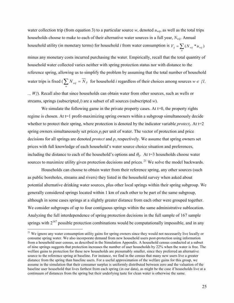
25

water collection trip (from equation 3) to a particular source w, denoted uwij, as well as the total trips

households choose to make to each of their alternative water sources in a full year, Nwij. Annual

household utility (in monetary terms) for household i from water consumption is ∑=w

wijwijij uNV )*(

minus any monetary costs incurred purchasing the water. Empirically, recall that the total quantity of

household water collected varies neither with spring protection status nor with distance to the

reference spring, allowing us to simplify the problem by assuming that the total number of household

water trips is fixed (∑ =w

ijwij NN for household i regardless of their choices among sources w ∈ {1,

.., W}). Recall also that since households can obtain water from other sources, such as wells or

streams, springs (subscripted j) are a subset of all sources (subscripted w).

We simulate the following game in the private property cases. At t=0, the property rights

regime is chosen. At t=1 profit-maximizing spring owners within a subgroup simultaneously decide

whether to protect their spring, where protection is denoted by the indicator variable protectj. At t=2

spring owners simultaneously set prices pj per unit of water. The vector of protection and price

decisions for all springs are denoted protect and p, respectively. We assume that spring owners set

prices with full knowledge of each household’s water source choice situation and preferences,

including the distance to each of the household’s options and θij. At t=3 households choose water

sources to maximize utility given protection decisions and prices. 21 We solve the model backwards.

Households can choose to obtain water from their reference spring, any other sources (such

as public boreholes, streams and rivers) they listed in the household survey when asked about

potential alternative drinking water sources, plus other local springs within their spring subgroup. We

generally considered springs located within 1 km of each other to be part of the same subgroup,

although in some cases springs at a slightly greater distance from each other were grouped together.

We consider subgroups of up to four contiguous springs within the same administrative sublocation.

Analyzing the full interdependence of spring protection decisions in the full sample of 167 sample

springs with 2167 possible protection combinations would be computationally impossible, and in any 21 We ignore any water consumption utility gains for spring owners since they would not necessarily live locally or consume spring water. We also incorporate demand from new household users post-protection using information from a household user census, as described in the Simulation Appendix. A household census conducted at a subset of nine springs suggests that protection increases the number of user households by 22% when the water is free. The welfare gains to protection for these new households are presumably smaller, since they preferred an alternative source to the reference spring at baseline. For instance, we find in the census that many new users live a greater distance from the spring than baseline users. For a useful approximation of the welfare gains for this group, we assume in the simulation that their consumer surplus is uniformly distributed between zero and the valuation of the baseline user household that lives farthest from each spring (in our data), as might be the case if households live at a continuum of distances from the spring but their underlying taste for clean water is otherwise the same.

26

case subgroups of approximately the size we use seem to correspond more closely to the relevant

social unit in both the pre-colonial period and under current Kenyan law, which delegates power over

water issues to local authorities. In sublocations where the number of springs is not divisible by four,

we created the largest possible groups (e.g., a location with seven springs was generally divided into

one group of four springs and one of three springs) unless a spring was located far from any other

spring (generally more than 1 km), in which case it was treated as isolated. The solution with groups

of up to four nearby springs is only an approximation to the full solution but we believe it is a fairly

close approximation: we have also run similar analyses with groups of one spring and two springs, in

addition to the four spring case we focus on below, and, while prices charged by private spring

owners do fall as the degree of competition increases, they fall at a declining rate and the social

welfare rankings of alternative property rights institutions are unchanged (not shown).

Spring owners’ profits are equivalent to the net present value of revenues, minus any spring

protection construction and maintenance costs (since the marginal cost of providing spring water is

zero) over a 15 year time horizon, and these costs are estimated at $1,405 and denoted K. The fact

that we have data on the actual local cost of the spring protection technology greatly simplifies the

solution of the spring owner’s problem. We find optimal spring owner prices conditional on

protection status either through a grid search (when computationally feasible) or the numerical

Nelder-Mead simplex method based on the profit functions’ first order conditions described below.22

We assume that neither spring owners nor planners can prevent resale of water, so pricing is linear in

the quantity collected and there is no price discrimination. To determine the Nash equilibrium choice

of protection with multiple springs, we estimate best responses to all possible protection/non-

protection combinations (at most 24 = 16 in subgroups of four springs) and search for a fixed point.

We consider the impact of changing property rights norms on spring investments and pricing

outcomes, holding constant policies for other water sources. This approach is realistic in the rural

Kenyan setting, where there is typically open access through public paths to naturally-occurring

rivers and lakes and most boreholes are sunk on public property such as schools or market centers so

people can collect water for free at these places. We assume this would continue to be possible.

We normalize social welfare to zero in the benchmark “status quo” case with common

property rights to water and no spring protection (Table 8, row 1 in panels A and B). We express

household utility and social welfare in U.S. dollar values on a per spring basis. We generally do not

present results on a per capita basis since the number of users can change with protection, but for a

22 Further details on the solution methods are in the supplementary Simulation Appendix available upon request.

27

rough sense of per capita gains, recall that the average baseline number of household spring users is

31 and households contain an average of 6.6 members, for roughly 200 persons per community.

We first consider the problem of a neoclassical social planner maximizing the utility of

households as indicated by revealed preference, and then a paternalistic social planner valuing each

DALY averted from spring protection at $125. We also evaluate various property rights institutions

from the perspective of each type of social planner. The decision problem of a social planner

maximizing revealed preference can be represented as follows, where WS denotes social welfare:

(6) ∑∑ ∑= = =

−=J

j

I

i

J

j

jijij

S

protectprotectKprotectVWMax

1 1 1

*)|( θ

and Vij(protect | θij) denotes household utility given that the planner is fully informed about true

household preference parameters, θij. In particular, given that households’ average revealed

preference valuation of health is equivalent to $23.68 per DALY averted, we assume the paternalistic

planner increases the utility value (βij) placed on spring protection approximately five-fold when

computing social welfare and making spring protection choices. We assume both the neoclassical

and paternalistic social planners are constrained to allow households to make their own water

collection choices based on revealed preference. (In section 5.4 below we also consider a third type,

an unconstrained paternalistic social planner who also determines household water collection

choices based on a welfare function that values each DALY averted from spring protection at $125.)

We next consider four forms of property rights – common property (the status quo described

above), “freehold” private property, Lockean private property, and modified Lockean (all defined

below) – and then consider two non-budget balancing mechanisms, public provision and vouchers.

We analyze each from the standpoint of both neoclassical and paternalistic social planners.

In freehold private property social norms, there are no restrictions on spring owners’

behavior. Private property rights are somewhat analogous to patents in this analysis. Creating private

property rights may spur potentially productive investments but induce static distortions since spring

owners have some market power in setting prices, given the travel costs households face in water

collection. To model this tradeoff, we assume spring owners set prices and make protection decisions

to maximize profits taking the decisions of neighboring spring owners as given, and we solve for the

Nash equilibrium. The owner of spring j maximizes

(7) { }∑∑= =

− −='

1' 1

**'

* *|),,(J

j

j

I

i

ijjjjijjjprotect

protectKpprotectprotectNpMaxj

θπ ,

28

where πj denotes profits and the owner takes others’ prices, p-j*, and protection decisions, protect-j

*,

as given. The double summation refers to all households at each spring j′ in the spring subgroup that j

belongs to, and Njij’ is the number of trips the household makes to spring j given the equilibrium

protection status and price decisions of other springs. This is solved subject to optimal non-

cooperative price setting: ),,(maxarg ***jjjj

pj pprotectprotectp

j

−−= π . The Nash equilibrium solution

is a vector of protection and price decisions for each spring, and consumption decisions for all

households, such that consumption decisions are optimal given protection and prices, and protection

and prices are optimal for each spring owner given other springs’ prices and protection decisions.

The simulations were run ten times, each with an independent draw of household preference

parameters (from mixed logit), and the results presented below are the average of the ten runs.23

5.3 Social Planner and Property Rights Simulation Results

The neoclassical social planner respecting households’ revealed preference valuations protects 29%

of springs, typically those with many baseline household users (Table 8, panel A, row 2). The net

social gain across all springs (protected and unprotected) is $351 per spring, or roughly $1.75 per

capita. A paternalistic social planner valuing a DALY averted by spring protection at $125 would

protect 63% of springs (Panel B, row 2). This is fewer than the 97% figure cited in section 5.1 for

isolated springs, since households can choose among multiple local springs in this case.

Under freehold private property, only 5% of spring owners find it profitable to protect their

spring (Table 8, panel A, row 3). The net present value of profits per spring owner is $420 and the

average price charged per water collection trip in these springs is $0.0027. While competition from

local springs does dampen potential price increases – the equilibrium price spring owners charge is

monotonically decreasing in the number of local competitor springs (if we compare the solution with

maximum group size of one, two, and four – not shown) – this average price remains quite expensive

for Kenyan households. For the typical household making 32 trips per week to a spring, this is

equivalent to $4.49 per year, or several days’ wages.

Freehold private property rights substantially reduce social welfare as measured by

household revealed preference relative to the status quo of communal property rights, with a social

welfare loss of $91 per spring. This finding may be a partial explanation why communal water rights

have been so durable in African settings like ours: they may simply yield higher social welfare than

23 A simulation run takes two days, so for practical reasons we use 10 runs (results from each available on request).

29

private property rights. The logic is straightforward: the dynamic gains from spring protection are

small since nearly all springs remain unprotected, but there are large static losses from households

walking further or choosing dirtier sources to avoid paying for water from springs located on private

land. The proportion of household trips to rivers and streams, the dirtiest local sources, increases by

45% relative to common property rights, and as a result average fecal contamination as measured by

E. Coli in collected water increases by 26 log points (from 4.66 to 4.92). Average walking time per

collection trip also rises by over a minute, from 11.6 to 12.9 minutes, and this amounts to over 100

extra hours per household each year.24

Freehold property rights lead to both under- and over- protection. On the one hand, only 13%

of the springs that would be protected by a neoclassical social planner are protected under private

property, but on the other hand some springs this social planner would not protect are protected under

private property. The inability of spring owners to capture the full consumer surplus of potential

users due to heterogeneity in valuations leads to under-protection, but a rent-stealing effect can lead

to over-protection, since land owners do not consider the negative impact of spring protection on

owners of competing nearby springs. The tendency of private owners with market power to focus on

the marginal consumer’s valuation of spring protection, rather than that of the average consumer,

could lead them to under- or over-protect springs depending on local demand patterns (Tirole 1988).

We do not present paternalistic social planner welfare outcomes for the freehold (or Lockean)

private property cases in Table 8, Panel B since they are not directly comparable to the communal

property outcomes. This is a product of the way we model the paternalistic planner’s social welfare

function in panel B: the planner places additional value on spring protection (essentially scaling up

the βij coefficient five-fold), but not on health gains from using other clean sources; a richer

simulation that incorporates the health impacts from the full range of sources awaits future research.

Yet a brief examination of panel B indicates that communal property will almost certainly continue

to yield higher social welfare in this case: while freehold private property leads to some spring

protection, it continues to generate increased average E. coli water contamination (as families turn

from relatively safe springs to more contaminated sources like rivers and streams due to high user

fees), and water collection walking times also rise considerably relative to common property.

24 In a small number of spring groups (3) there are multiple Nash equilibria in the freehold private property rights case. Here we assume there is coordination on the equilibrium that maximizes social welfare, although given the small number of cases other equilibrium selection rules do not change the main results. Thus the social welfare outcomes in the freehold private property rights case (where multiple equilibria sometimes arise) likely represent upper bounds, yet despite this there are substantial welfare losses relative to communal property.

30

It is also worth considering other private property rights institutions beyond the stylized

extremes of common property and freehold private property, since actual social norms are often more

complex. Locke (1689 [2002]) argued that people acquire property rights in land when they mix their

labor with it, for example by clearing land or planting a crop. This element of property rights is

common in rural Africa and elsewhere. For example, in Ghana actively farming a plot is critical to

securing property rights (Goldstein and Udry 2005) and clearing land is traditionally necessary for

establishing rights to plots at the margin of Amazon tropical forests. A “Lockean” private property

norm in our context would only permit spring owners to charge positive prices if they had invested in

spring protection. In the model, the spring owner’s profit maximizing condition is similar but now

the price is constrained to be pj=0 if protectj=0.

Historically, some legal systems seem to have evolved from common property for water

towards the Lockean norm; for instance, despite the fact that water sales are discouraged by several

hadith (see Caponera 2006), certain Islamic legal traditions evolved to allow the builders of wells

and irrigation canals to charge for access to the water made available by their investments (Mawardi

1901: 316, Wanasharisi 1909: 285). Lockean norms may also be emerging in another Kenyan

region: local officials in Nyanza province do sometimes permit spring owners to charge for access to

spring water once they have invested in spring protection (personal communication with Scott Lee).

Under Lockean property rights, spring owners’ continued inability to price discriminate and

thus capture the full consumer surplus from protection leads to under-protection, as in the freehold

private property case. On the other hand, the possibility that protecting a spring allows owners to

capture not just the valuation on spring protection but also part of the surplus from consuming

unprotected water could lead to over-protection. In practice, there is substantial under-protection

(Table 8, panel A, row 4). The simulations suggest Lockean private property rights yield somewhat

higher investment in water infrastructure than freehold private property: 12% of owners now find it

profit maximizing to invest in spring protection. Although social welfare (using revealed preference

valuation) remains lower than the status quo, Lockean rights are marginally better for welfare than

freehold private property: the average annual social welfare loss per community is only $43, average

fecal contamination increases by just 4 log points and average walking time rises slightly, from 11.6

to 12.3 minutes. Yet the increase in both fecal contamination and walking time suggests that a

paternalistic planner would also likely prefer common property to Lockean property norms.25

25 It is possible that disaggregating trips by water use (something we are unfortunately unable to do with our data) could partially affect the conclusion, since households would have the option of purchasing some drinking water at springs and collecting water for other uses elsewhere. We leave this for future research.

31

A “modified Lockean” private property rights regime would permit spring owners to charge

for water from spring protection infrastructure as long as they also allowed free unimpeded access to

unprotected water from the spring. In our setting, a system of modified Lockean property rights could

be achieved simply by requiring owners who protect springs to allow some water to flow out of the

pipe and away from the protected spring, where it becomes a pool of unprotected spring water

exposed to the environment that anyone can access for free. In this case, the spring owner’s profit

maximizing condition is equivalent to that under the Lockean case, with the critical change that

under protection the spring owner must now take into account that households have the choice of

continuing to consume unprotected spring water at price pj=0 at the source. This regime generates a

Pareto improvement over the common property status quo, since the availability of free unprotected

spring water shields households from the utility losses experienced under the other private property

cases, and spring owners cannot be worse off than under common property.

This regime performs best within the set of set of budget-neutral social norms. Under

modified Lockean property rights, 2% of springs are protected (Table 8, panel A, row 5). Six percent

of the springs a neoclassical social planner would protect are protected in this case, while only 1% of

springs the neoclassical planner would not protect are protected (not shown). While this form of

property rights is far from attaining the social optimum, it incentivizes spring owners to perform

some socially beneficial spring protection while leaving no households worse off.

The paternalistic planner would also prefer this modified Lockean system to common

property. Although average ln(E. Coli) levels are the same to two decimal places in Table 8, they are

in fact lower by 0.002 under the modified Lockean system. Yet these social welfare gains from

modified Lockean rights are sufficiently small that it is perhaps unsurprising that there has been

limited institutional innovation along these lines in Kenya, given the transition costs of changing

property norms, enforcing charges for protected sources, preventing owners from impeding access to

unimproved water, and any engineering costs of allowing spring water to freely run off.

Public funding, either through direct government provision or vouchers, performs much

better than the budget-neutral property rights norms considered above. Consider the impact of public

funding by a hypothetical benevolent government that had access only to distortionary taxation and

knows only the distribution of preferences in the population, F(θij), not individual household

preferences in each community. Consider first a policymaker that maximizes household revealed

preference welfare. This policymaker’s optimization problem is the following, where DW denotes the

deadweight loss of taxation per dollar of revenue raised:

32

(8) ∑∑ ∑= = =

+−=J

j

I

i

J

j

jijij

P

protectprotectKDWFprotectVWMax

1 1 1

**)1())(|(~

θ

Assuming that DW=0.3 (Ballard et al. 1985)26, the government protects 22% of springs

(Table 8, panel A, row 6) but there is some misallocation of protection: 49% of those springs the

neoclassical social planner would optimally protect get protected, and 12% of those the planner

would not protect (not shown). The welfare gain per spring is $131, less than the $351 gain attained

by a social planner, due to the tax distortion and the misallocation of protection across springs due to

policymakers’ limited information on households’ preferences. A paternalistic government that

values health gains from protection at $125/DALY would protect 67% of springs (panel B, row 6),

coming much closer to the corresponding social planner than any of the budget-neutral approaches.

Finally, consider a regime where the government does not protect springs directly but rather

provides households with vouchers for protected spring water which they can pay to spring owners,

and which spring owners can then exchange for a fixed payment from the government. The

government optimally sets the voucher payment taking into account the later non-cooperative

protection decisions of private spring owners. We assume that the policymaker only knows the

distribution of water preferences in the entire population, but that spring owners still have perfect

knowledge of local preferences. Spring owners are assumed to be restricted from charging top-up

fees to water users, so households’ ex post decisions on which water sources to use are efficient. The

policymaker maximizes social welfare WV by setting the uniform voucher price pv:

(9) { } { } ∑∑∑∑ ∑= == = =

−+=J

j

I

i

ijvijv

J

j

I

i

J

j

vjijvij

V

pFpprotectNpDWpFpprotectVWMax

v 1 1

*

1 1 1

** ))(|)((*)())(|)((~

θπθ

subject to spring owner protection decisions being profit maximizing:

(10) )(maxarg **vjj pprotect π= ,

where spring owner profits are given by { }∑∑= =

− −='

1' 1

*' *|)0,,(

J

j

j

I

i

ijjjjijvj protectKprotectprotectNp θπ .

For a government that respects household revealed preferences, and again faces 30%

deadweight loss, the optimal voucher price is $0.0010 per trip to a protected spring (much less than

the price charged in the freehold private property rights case), and social welfare gains per spring

under water vouchers are $138 (or roughly $0.69 per capita). 12% of spring owners protect their

springs (Table 8, panel A, row 7), still short of the social optimum, but there is less misallocation of

protection in this case, since spring owners with good information on local demand are the ones

26 The main results are unchanged under the assumption that DW=0.5 (results not shown).

33

making protection decisions: only 3% of the sample springs the social planner would not protect get

protected here (not shown in the table). This policy improves social welfare substantially relative to

all the budget-neutral cases, and social welfare is comparable to government investment.

A paternalistic policymaker with health valuation at $125/DALY sets a uniform voucher price

of $0.0041 (Table 8, panel B, row 7), four times higher than the previous price level, and as a result

65% of spring owners choose protection. For the paternalistic planner, we estimate slightly higher

spring protection and social welfare under government provision than under vouchers. We conjecture

that this is, in part, because raising the voucher price to increase protection above the 65% level

associated with vouchers does not effectively target those springs a social planner would protect but

instead leads to increased protection of other springs due to rent-stealing effects (recall that spring

owners make protection decisions in the voucher case). However, both government cases perform

much better than any budget-neutral property rights system under both the neoclassical social planner

and the paternalistic planner.

5.4 The Determinants of Optimal Property Rights Institutions

If households’ spring protection valuation increased by 20%, freehold private property rights and

Lockean private property rights norms would both become preferable to common property norms

(not shown, available on request). If these valuations increase with income, and the income elasticity

of demand for health is greater than one (as in Hall and Jones 2007), this implies that per capita

income growth of less than 20% in this region could make private property rights more attractive

than the current norm of communal access. If this finding that private property rights are optimal at

higher income levels holds more broadly, it could help explain the strong cross-sectional relationship

documented between institutions and income levels, and suggests it would be risky to assume that

causality always runs from stronger property rights protection to higher income levels (North 1990).

The social welfare ordering of the public cases (government investment and vouchers) versus

private property rights cases is remarkably robust to alternative assumptions about households’

monetary valuation of spring protection (and equivalently, the value of water collectors’ time). In

results not presented in Table 8, public investment and vouchers both yield far higher social welfare

than any of the private property rights cases when household valuation for spring protection is 2, 3, 4,

or 5 times larger than the revealed preference estimates. Note that the evaluation of social welfare by

a planner in this exercise is equivalent to the case of the unconstrained paternalistic social planner

mentioned above, in which the planner not only makes investment and pricing decisions but also

determines household water collection decisions.

34

Yet for household spring protection valuations sufficiently close to zero (such that zero

protection investment is socially optimal), it is straightforward to show that communal property

rights yield social welfare at least as high as all other property rights norms, including the

government cases. It thus seems likely that communal property norms for water were in fact socially

optimal when they emerged in pre-colonial Kenya, a historical period when income was much lower,

the spring protection technology was costlier, and population density – and thus water contamination

levels and the number of potential users among whom to share fixed investment costs – was lower.

Finally, the analysis above abstracts from transaction costs in collecting water user fees, but

these are likely to be large under private property norms. In particular, it may be expensive for spring

owners to monitor the amount of water that households collect, and these transaction costs would

reduce social welfare benefits. More generally, there are likely to be non-trivial transition costs in

moving from any one system to another, and these may be particularly large for water privatization

that runs against traditional communal social norms, as in rural Kenya. Certain cases may also have

real-world advantages that are not modeled here, especially with regards to ongoing incentives for

spring maintenance over time. For instance, an inept or corrupt government’s investment program

may collapse after a short time, in which case a voucher system (where maintenance remains with

private spring owners) or the modified Lockean case could be preferable.

6. Discussion and conclusion

Spring protection dramatically improved source water quality in a rural African setting, reducing

fecal contamination by two thirds and both home water contamination and child diarrhea by one

quarter. By capitalizing on changes in water source choice in response to spring protection, we

develop revealed preference estimates of willingness to pay for improved water quality. Because of

the experimental research design, these travel cost estimates are not subject to many typical

econometric concerns, and can be used to validate the reliability of stated preference estimates.

Revealed preference estimates of spring protection valuation are far below stated preference

estimates and, assuming people understand the effect of spring protection on health, imply valuations

of only US$23.68 per disability adjusted life year (DALY), roughly one fifth of the valuations

typically used by public health planners. The estimated valuations are consistent with models such as

Hall and Jones (2007) in which the elasticity of demand for health is much greater than one.

Using structural econometric methods in tandem with the spring protection experiment, we

carry out counterfactual simulations based on estimated household revealed preference valuations for

spring protection, to examine the consequences of alternative property rights norms for water.

35

Existing social norms allowing communal access to naturally occurring springs yield higher social

welfare than private property norms in this setting, providing a rationale for why communal water

rights have persisted in this rural African region. Simulations suggest that private property becomes

more attractive than communal norms when health valuations reach a sufficient level, which seems

like to occur as incomes rise. We also conjecture (as argued in Platteau 2000) that higher population

densities, or other factors that affect water scarcity would also boost local willingness to pay for

water and thus the attractiveness of freehold private property rights relative to communal property

norms. Water scarcity is an increasingly pressing issue in India, for instance, where expanding

irrigation and urban water use is leading to rapid drops in the water table.

Many historical analyses of movements from common property to private property

institutions, such as British land enclosures (Allen 1982), may well find they are associated with

increased social welfare. Yet this is not inconsistent with arguments that common property

institutions are in fact sometimes optimal in other contexts. If health valuations rise with income, and

there are substantial costs to shifting to new property rights institutions, then if income follows a

stochastic process, societies may only elect to change property rights norms at income levels far

above those at which such shifts appear statically efficient. Such changes may also be delayed in

practice if political institutions make it impossible for “winners” from the new property rights to

credibly compensate “losers”, or they can only be undertaken with the consent of supra-majorities.

Our property rights simulations suggest, that even at current Kenyan income levels, new

institutions and policies could potentially be layered onto existing common property norms to

improve social welfare, including government provision or vouchers through which the government

pays spring owners based on the number of water users, or by allowing spring owners to charge for

improved water while maintaining access to unimproved sites, what we call the modified Lockean

approach. In our setting, the Government of Kenya and foreign aid donors are in fact protecting

increasing numbers of springs over time while maintaining common property access. The analysis in

this paper suggests their approach is reasonable given current technology and household preferences.

36

References

Acemoglu, Daron, Simon Johnson, and James Robinson. (2001). “The Colonial Origins of Comparative Development: An Empirical Investigation”, American Economic Review, 91(5), 1369-1401.

Adams, Martin, Sipho Sibanda and Stephen Turner (1999). “Land Tenure Reform and Rural Livelihoods in Southern Africa,” Natural Resources Perspectives v39.

Allen, Robert C. (1982). “The Efficiency and Distributional Consequences of Eighteenth Century Enclosures”, Economic Journal, 92, 937-953.

Angrist, J., G. Imbens, and D. Rubin (1996), “Identification of causal effects using instrumental variables,” Journal of the American Statistical Association 91(434), 444-472.

Aziz, K., et al. (1990), “Reduction in diarrhoeal diseases in children in rural Bangladesh by environmental and behavioural modifications,” Transactions of the Royal Society of Tropical

Medicine and Hygiene 84(3), 433-438. Ballard, Charles L., John B. Shoven, and John Whalley. (1985). “General equilibrium computations

of the marginal welfare costs of taxes in the United States”, American Economic Review, 75(1), 128-138.

Bartlett, Roger (ed.). (1990). Land Commune and Peasant Community in Russia: Communal Farms

in Imperial and Early Soviet Society. New York: St. Martin's Press. Bateman, I. and K. G. Willis, (1999), Valuing Environmental Preferences: The Theory and Practice

of the Contingent Valuation Method in the US, EU and Developing Countries. Oxford Univ. Press: New York.

Berry, Steven, James Levinsohn, and Ariel Pakes. (1995). “Automobile Prices in Market Equilibrium”, Econometrica, 63(4), 841-890.

Black, R.E. (1998), “Therapeutic and preventive effects of zinc on serious childhood infections diseases in developing countries,” American Journal of Clinical Nutrition 68(suppl.), 476-9s.

Bruhn, Miriam and David McKenzie. (2008). “In pursuit of balance: Randomization in practice in development field experiments”, World Bank Policy Research Working Paper #4752.

Bryce, J. et al. (2005), “WHO estimates of the causes of death in children,” Lancet 365: 1147-52. Cameron, T.A. (1992), “Combining contingent valuation and travel cost data for the valuation of

nonmarket goods,” Land Economics, 68(3):302-317. Caponera, Dante A.. (2006). “Ownership and transfer of water and land in Islam.” Updated 8

June 2006. IDRC: Science for Humanity. <www.crdi.ca/es/ev-93957-201-1-DO_TOPIC.html> Accessed December 26, 2008.

Carson, R.T., N.E. Flores, K. Martin, and J. Wright (1996), Contingent valuation and revealed preference methodologies: Comparing the estimates for quasi-public goods, Land Economics, 72(1): 80-99.

Choe, K. (1996) “The economic benefits of surface water quality improvements in developing countries: A case study of Davaeo, Philippines” Land Economics 72(4): 519-537

Curtis, V., S. Cairncross, and R. Yonli. (2000), “Domestic Hygiene and diarrhea—Pinpointing the problem.” Tropical Medicine and International Health 5(1):22–32.

De Soto, Hernando. (1989) The Other Path: The Invisible Revolution in the Third World. New York: Harper & Row.

Deaton, Angus, Jane Fortson, and Robert Tortora. (2008). “Life (evaluation), HIV/AIDS, and death in Africa”, unpublished working paper, Princeton University.

Demographic and Health Surveys (DHS) (2003). Kenya Demographic and Health Household Survey Data. MEASURE DHS, Macro International Inc., Calverton, MD.

Diamond, P.A. and J. A. Hausman, (1994), “Contingent valuation: Is some number better than no number?” Journal of Economic Perspectives, 8(4),45-64

37

Esrey S.A. (1996), “Waste, water and well-being: A multicountry study,” American Journal of

Epidemiology 143(6), 608-22. Fafchamps, Marcel and Sarah Gavian, (1996). “Land Tenure and Allocative Efficiency in Niger,”

American Journal of Agricultural Economics, 78(2): 460-471. Faruqui, Naser I., Asit K. Biswas, and Murad J. Bino, eds.. (2001). Water Management in Islam.

New York: United Nations University Press. Fewtrell, L. et al. (2005), “Water, sanitation, and hygiene interventions to reduce diarrhoea in less

developed countries: A systematic review and meta-analysis,” Lancet Infectious Diseases 5, 42-52.

Goldstein, Markus, and Christopher Udry. (2005). “The Profits of Power: Land Rights and Agricultural Investment in Ghana”, unpublished manuscript World Bank and Yale Univ.

Griffin, C. et al (1995) “Contingent valuation and actual behavior: predicting connections to new water systems in the state of Kerala, India” World Bank Economic Review 9(3): 373-395

Hall, R., and C.I. Jones, (2007), “The Value of Life and the Rise in Health Spending", Quarterly

Journal of Economics, 122(1): 39-72. Hoy, M. and Jimenez, E., (2006), "Property Rights and the Urban Environment: Local Public Goods

in Indonesian Cities," Working Paper 2006-9, University of Guelph, Dept. of Economics. Huttly S.R.A. et al. (1987), “The epidemiology of acute diarrhea in a rural community in Imo State,

Nigeria,” Transactions of the Royal Society of Tropical Medicine and Hygiene 81, 865-70. Imbens, Guido, and Jeffrey M. Wooldridge. (2008). “Recent developments in the econometrics of

program evaluation”, NBER Working Paper #14251. Kay, D., J.M. Fleisher, R.L. Salmon, F. Jones, M.D. Wyer, A.F. Godfree, Z. Zelenauch-Jacquotte

and R. Shore, (1994). Predicting likelihood of gastroenteritis from sea bathing: results from randomised exposure. Lancet 344, pp. 905–909.

Kirkwood, B.R. (1991). “Diarrhea”, pp. 134-157, in R.G. Feacham and D.T. Jamison, eds., Disease

and Mortality in Sub-Saharan Africa. New York: Oxford Univ. Press for World Bank. Kremer, Michael, Edward Miguel, Clair Null, and Alix Zwane. (2008). “Trickle down: Diffusion of

chlorine for drinking water treatment in Kenya”, unpublished working paper, U.C. Berkeley. Larson, Douglas M. 1993. "Separability and the Shadow Value of Time," American Journal

of Agricultural Economics, 75 (August), pp. 572-577. Lenehan, A. and J. Martin (1997), “Spring protection in southern KwaZulu Natal,” presented at 23rd

Water, Engineering, & Development Centre Conference on Affordable Water Supply & Sanitation, Durban.

Locke, John. (1689 [2002]). The 2nd Treatise of Government and a Letter Concerning Toleration. Dover.

Lopez, A.D., et al., eds. (2006). Global Burden of Disease and Risk Factors, Washington DC: World Bank and Oxford University Press.

Madajewicz, M., et al. (2007) “Can information alone change behavior? Response to arsenic contamination of groundwater in Bangladesh”, J. of Development Economics, 84, 731-54.

Mawardi, Ali ibn Muhammad. Traité de droit public musulman, tr. L. Ostrorog. Paris: Leroux, 1900-1901. (Cited in Caponera, Dante A. above.)

McFadden, D. (1974), “Conditional logit analysis of qualitative choice behavior”, in P. Zarembka, ed., Frontiers in Econometrics, Academic Press, New York, pp. 105-142.

McKean, J. R., D. Johnson, and R. Walsh, (1995) "Valuing time in travel cost demand analysis: An empirical investigation," Land Economics, 71(1).

Mu, X., D., Whittington, and J. Briscoe, (1990), “Modelling village water demand behavior: A discrete choice approach,” Water Resources Research 26(4), 521-529.

38

Mumma, Albert. (2005). “Kenya’s new water law: an analysis of the implications for the rural poor”, paper presented at the Workshop on African Water Laws: Plural Legislative Frameworks for

Rural Water Management in Africa, January 2005, Johannesburg, South Africa. Mwami, J. (1995), “Spring protection/sustainable water supply,” presented at Water, Engineering,

and Development Centre Conference on Affordable Water Supply and Sanitation, Kampala. North, Douglas C. (1990). Institutions, Institutional Change and Economic Performance. Cambridge;

New York: Cambridge University Press. Ostrom, Elinor. (1990). Governing the Commons: The Evolution of Institutions for Collective Action.

Cambridge University Press. Peters, Pauline E. (2007). “Challenges in land tenure and land reform in Africa: An anthropological

perspective,” CID Working Paper No. 141. Platteau, J-P. (2000). Institutions, Social Norms, and Economic Development. Harwood. Rosado, Maria et al (2006), “Combining averting behavior and contingent valuation data: an

application to drinking water treatment in Brazil,” Environment and Development

Economics, 11:729-746 Sachs J. (2002), Macroeconomics and health: Investing in health for economic development. World

Health Organization: Geneva. Shillcutt, Samuel, Damian Walker, Catherine Goodman, and Anne Mills. (2007). “Cost-effectiveness

in low- and middle-income countries: A review of the debates surrounding decision rules”, iHEA 6th World Congress: Explorations in Health Economics Paper.

Tirole, Jean. (1988). The Theory of Industrial Organization. MIT Press: Cambridge. Todd, Petra, and Kenneth Wolpin. (2006). “Assessing the Impact of a School Subsidy Program in

Mexico: Using a Social Experiment to Validate a Dynamic Behavioral Model of Child Schooling and Fertility”, American Economic Review, 96(5), 1384-1417.

Train, K. (2003). Discrete Choice Methods with Simulation. Cambridge Univ. Press: Cambridge. Train, K.,(1999). “Mixed Logit Models of Recreation Demand,” in C. Kling and J. Herriges, eds.,

Valuing the Environment Using Recreation Demand Models, Elgar Press. UNDP (2007) Human Development Report 2007/2008: Fighting Climate Change: Human Solidarity

in a divided world, UNDP: New York. UNEP (United Nations Environment Program) (1998), Sourcebook of alternative technologies for

freshwater augmentation in Africa, Osaka: UNEP. Wansharisi, Ahmad ibn Yahyá. La pierre de touche des fétwas, tr. É. Amar. Paris: Leroux, 1909.

(Cited in Caponera, Dante A. above.) Were, Gideon. (1967). A History of the Abaluyia of Western Kenya. East African Publish.: Nairobi. Were, Gideon (ed.). (1986). Socio-cultural Profile of Busia District. Government of Kenya:

Ministry of Planning and National Development. Whitehead, J. C. (2006), “A comparison of contingent valuation method and random utility model

estimates of the value of avoiding reductions in King Mackerel bag limits," Applied

Economics, 38(15):1725-1735. Whittington, D., X. Mu, and R. Roche (1990) “Calculating the value of time spent collecting water:

Some estimates for Ukunda, Kenya,” World Development 18(2), 269-280. World Bank (1993). World Development Report. New York: Oxford University Press.

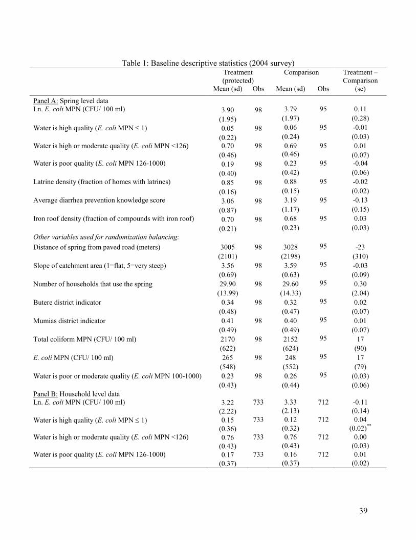
39

Table 1: Baseline descriptive statistics (2004 survey)

Treatment (protected)

Comparison Treatment – Comparison

Mean (sd) Obs Mean (sd) Obs (se)

Panel A: Spring level data Ln. E. coli MPN (CFU/ 100 ml) 3.90 98 3.79 95 0.11 (1.95) (1.97) (0.28) Water is high quality (E. coli MPN ≤ 1) 0.05 98 0.06 95 -0.01 (0.22) (0.24) (0.03) Water is high or moderate quality (E. coli MPN <126) 0.70 98 0.69 95 0.01 (0.46) (0.46) (0.07) Water is poor quality (E. coli MPN 126-1000) 0.19 98 0.23 95 -0.04 (0.40) (0.42) (0.06) Latrine density (fraction of homes with latrines) 0.85 98 0.88 95 -0.02 (0.16) (0.15) (0.02) Average diarrhea prevention knowledge score 3.06 98 3.19 95 -0.13 (0.87) (1.17) (0.15) Iron roof density (fraction of compounds with iron roof) 0.70 98 0.68 95 0.03 (0.21) (0.23) (0.03) Other variables used for randomization balancing:

Distance of spring from paved road (meters) 3005 98 3028 95 -23 (2101) (2198) (310) Slope of catchment area (1=flat, 5=very steep) 3.56 98 3.59 95 -0.03 (0.69) (0.63) (0.09) Number of households that use the spring 29.90 98 29.60 95 0.30 (13.99) (14.33) (2.04) Butere district indicator 0.34 98 0.32 95 0.02 (0.48) (0.47) (0.07) Mumias district indicator 0.41 98 0.40 95 0.01 (0.49) (0.49) (0.07) Total coliform MPN (CFU/ 100 ml) 2170 98 2152 95 17 (622) (624) (90) E. coli MPN (CFU/ 100 ml) 265 98 248 95 17 (548) (552) (79) Water is poor or moderate quality (E. coli MPN 100-1000) 0.23 98 0.26 95 (0.03) (0.43) (0.44) (0.06) Panel B: Household level data Ln. E. coli MPN (CFU/ 100 ml) 3.22 733 3.33 712 -0.11 (2.22) (2.13) (0.14) Water is high quality (E. coli MPN ≤ 1) 0.15 733 0.12 712 0.04 (0.36) (0.32) (0.02)** Water is high or moderate quality (E. coli MPN <126) 0.76 733 0.76 712 0.00 (0.43) (0.43) (0.03) Water is poor quality (E. coli MPN 126-1000) 0.17 733 0.16 712 0.01 (0.37) (0.37) (0.02)

40

Treatment (protected)

Comparison Treatment – Comparison

Mean (sd) Obs Mean (sd) Obs (se)

Respondent years of education 5.71 731 5.66 717 -0.05 (3.61) (3.60) (0.23) Children under age 12 in the compound 4.04 736 3.93 719 0.11 (2.48) (2.46) (0.14) Iron roof indicator 0.70 735 0.68 717 0.03 (0.46) (0.47) (0.03) Walking distance to closest water source (minutes) 8.74 725 8.03 714 0.71 (8.40) (6.82) (0.49) Water collection trips per week by household 48.03 733 47.99 716 0.04 (36.51) (38.48) (2.51) Ever collects drinking water at “reference” spring indicator 0.82 661 0.80 668 0.02 (0.38) (0.40) (0.03) Multi source user (uses sources other than reference spring) 0.45 732 0.44 715 0.00 (0.50) (0.50) (0.04) Fraction of respondent water trips to “reference” spring 0.72 655 0.71 663 0.01 (0.41) (0.42) (0.04) Rates water at the spring “very clean” – rainy season 0.33 736 0.33 719 0.00 (0.47) (0.47) (0.04) Rates water at the spring “very clean” – dry season 0.74 736 0.74 719 -0.01 (0.44) (0.44) (0.03) Fraction of water trips by those under age 12 0.10 727 0.10 711 -0.00 (0.20) (0.20) (0.01) Water storage container in home was covered 0.90 673 0.93 656 -0.03 (0.30) (0.26) (0.02)** Yesterday's drinking water was boiled indicator 0.25 731 0.29 711 -0.03 (0.43) (0.45) (0.02) Respondent diarrhea prevention knowledge score 3.06 736 3.19 719 -0.13 (2.14) (2.26) (0.15) Respondent said “dirty water” causes diarrhea 0.68 736 0.67 719 0.01 (0.47) (0.47) (0.03) Household has soap in the home 0.91 733 0.91 717 0.00 (0.28) (0.29) (0.02) Panel C: Child demographics and health Child age (years) 1.70 1047 1.72 995 -0.02 (0.95) (0.97) (0.04) Child male (=1) 0.52 1047 0.53 995 -0.01 (0.50) (0.50) (0.02) Child had diarrhea in past week indicator 0.23 996 0.20 961 0.03 (0.42) (0.40) (0.02) Child height (cm) 76.10 870 76.13 835 -0.03 (11.67) (12.16) (0.57) Child weight (kg) 9.98 864 10.02 810 -0.05 (3.04) (3.09) (0.16)

Notes: The treatment springs were later protected (in 2005). Huber-White robust standard errors are clustered at spring level when using household level data, significant at * 90% ** 95% *** 99% confidence. Reference spring is based on spring user lists. Children in Panel C were under age 3 at baseline or were born since then.

41

Table 2: Spring protection source water quality impacts (2004-2007) Dependent variable: ln(Spring water E. coli MPN) Water clarity

(observed) Water yield (observed)

(1) (2) (3) (4) (5) Treatment (protected) indicator -1.07 -1.04 -1.10 0.26 -0.06 (0.27)*** (0.23)*** (0.24)*** (0.07)*** (0.06) Baseline ln(Spring water E. coli MPN) 0.99 1.01 (0.07)*** (0.08)*** Baseline ln(Spring water E. coli MPN) * Treatment indicator

-0.17 (0.12)

-0.16 (0.13)

Baseline latrine density -0.23 (0.59) Baseline latrine density * Treatment indicator

0.89 (1.75)

Baseline diarrhea prevention score -0.03 (0.07) Baseline diarrhea prevention score *Treatment indicator

-0.29 (0.24)

Baseline boiled water yesterday density 0.48 (0.65) Baseline boiled water yesterday density *Treatment indicator

0.94 (1.51)

Baseline mother’s years of education density -0.04 (0.05) Baseline mother’s years of education density *Treatment indicator

0.06 (0.14)

Treatment group 1 (phased in early 2005) -0.29 (0.20) Treatment group 2 (phased in late 2005) -0.21 (0.17) R2 0.30 0.43 0.45 0.13 0.13 Observations 726 726 726 478 478 Mean (s.d.) of dependent variable 3.63

(1.95) 3.63 (1.95)

3.63 (1.95)

0.71 0.73

Notes: Estimated using OLS. Huber-White robust standard errors are presented (clustered at the spring level), significantly different than zero at * 90% ** 95% *** 99% confidence. There are 184 spring clusters with data for some of the four survey rounds (2004, 2005, 2006, 2007). MPN stands for “most probable number” coliform forming units (CFU) per 100ml. Average diarrhea prevention knowledge calculated as average of demeaned sum of number of correct responses given to the open ended question “to your knowledge, what can be done to prevent diarrhea?” Outcomes in columns 4 and 5 are enumerator assessments of spring water clarity and the spring’s water yield. All variables that are interacted with the treatment indicator are de-meaned. Time (survey round and wave) fixed effects are included in all regressions but not reported, as are all variables used to balance the initial randomization into treatment and comparison groups. When interactions are included, baseline variables are interacted with time indicators and treatment group indicators in addition to the treatment (protected) indicator. These coefficients not reported. Baseline iron roof density and its interaction with the treatment indicator (in col. 3) are included as additional control variables (not shown in the table). The -1.07 effect in column 1 is equivalent to a 66% reduction in E. Coli fecal coliform units per 100ml.

42

Table 3: Spring protection household water quality impacts (2004-2007)

Dependent variable: ln(Home water E. coli MPN)

(1) (2) (3) Treatment (protected) indicator -0.27 -0.29 -0.67 (0.15)* (0.19) (0.27)** Baseline ln(Spring water E. coli MPN) 0.01 0.03 0.035 (0.05) (0.05) (0.05) Baseline multi-source user -0.29 -0.27 (0.16)* (0.17) Baseline multi-source user * Treatment indicator 0.04 0.06 (0.25) (0.26) Baseline latrine density -0.73 -0.73 -0.02 (0.32)** (0.31)** (0.60) Baseline latrine density * Treatment indicator 1.42 (1.01) Baseline diarrhea prevention score -0.02 -0.03 -0.05 (0.02) (0.02) (0.04) Baseline diarrhea prevention score * Treatment indicator -0.05 (0.06) Baseline boiled water yesterday indicator 0.17 0.16 0.29 (0.08)** (0.08)** (0.15)* Baseline boiled water yesterday indicator * Treatment indicator 0.52 (0.28)* Baseline mother’s years of education 0.00 0.00 0.02 (0.01) (0.01) (0.02) Baseline mother’s years of education * Treatment indicator 0.02 (0.04) Treatment group 1 (phased in early 2005) 0.00 -0.14 -0.01 (0.14) (0.18) (0.27) Treatment group 2 (phased in late 2005) -0.10 -0.12 -0.16 (0.12) (0.15) (0.27) R2 0.04 0.04 0.05 Observations (spring clusters) 4343 (184) 4343 (184) 4343 (184) Mean (s.d.) of dependent variable in comparison group 3.00 (2.27) 3.00 (2.27) 3.00 (2.27)

Notes: Estimated using OLS. Huber-White robust standard errors (clustered at the spring level) are presented, significantly different than zero at * 90% ** 95% *** 99% confidence. MPN stands for “most probable number” coliform forming units (CFU) per 100ml. Additional control variables are: season fixed effects, number of children under 12 living in the home, home has iron roof indicator, iron roof density within spring community. When differential treatment effects are reported in column 3, we also include interactions of these control variables with the treatment (protected) indicator (not shown in the table). Baseline spring water quality, latrine density, diarrhea prevention score, and mother’s education are de-meaned. Time (survey round and wave) fixed effects included in all regressions but not reported, as are all variables used to balance the initial randomization into treatment and comparison groups. When interactions are included, baseline variables are interacted with time effects and treatment group indicators, in addition to interactions with treatment (protected) indicator. These coefficients not reported in the table. The -0.27 effect in column 1 is equivalent to a 24% reduction in E. Coli fecal coliform units per 100ml.

43

Table 4: H

ealth outcom

es for children under age three at baseline or born since 2004 (2004-2007 data)

------------Dependent variable: Diarrhea in past w

eek ------------

Dependent variable

Weight (kg)

Dependent variable

Body mass index,

BMI (kg/m

2 )

(1)

(2)

Probit

(3)

(4)

(5)

(6)

(7)

(8)

(9)

(10)

Treatment (protected) in

dicator

-0.045

***

-0.044

**

-0.045

* -0.047

**

-0.090

***

-0.032

0.06

5 0.09

3 0.21

0.27

(0.012)

(0.020)

(0.023)

(0.023)

(0.029)

(0.039)

(0.076)

(0.100)

(0.13)

* (0.17)

Treatment (protected) in

dicator *

M

ale

0.08

3**

(0.040)

-0.054

(0.120)

-0.12

(0.19)

Treatment (protected) in

dicator *

Baseline latrine density

0.10

5 (0.119)

Treatment (protected) in

dicator *

B

aseline diarrhea prevention score

-0.008

4 (0.0073)

Treatment (protected) in

dicator *

B

aseline mother’s years of educatio

n

0.00

23

(0.0044)

Child fixed effects

No

No

Yes

Yes

Yes

Yes

Yes

Yes

Yes

Yes

Treatment g

roup fixed effects

No

No

Yes

Yes

Yes

Yes

Yes

Yes

Yes

Yes

Month of year controls

No

No

Yes

Yes

Yes

Yes

Yes

Yes

Yes

Yes

Gender-age controls

No

No

No

Yes

Yes

Yes

Yes

Yes

Yes

Yes

R2

0.00

- 0.53

0.53

0.53

0.53

0.96

0.96

0.69

0.69

Child-year observations

6750

6749

6749

6660

6660

6601

5736

5736

5646

5646

Mean (s.d.) of the dependent variable in th

e comparison group

0.19

(0.39)

0.19

(0.39)

0.19

(0.39)

0.19

(0.39)

0.19

(0.39)

0.19

(0.39)

11.36

(3.50)

11.36

(3.50)

17.0

(2.2)

17.0

(2.2)

Notes: C

olum

n 2 estim

ated using probit (marginal effects presented), colum

ns 1 and 3-10 estim

ated using OLS. H

uber-W

hite robust standard errors

(clustered at the spring level) are presented, significantly different th

an zero at * 90%

** 95% *** 99%

confidence. Data from

all four survey rounds (2004,

2005, 2006, 2007), sam

ple restricted to

children under age three at baseline (in 2004) and child

ren born since 2004. Diarrhea defined as th

ree or m

ore

“looser than normal” stools with

in 24 hours at any time in th

e past week. The gender-age controls in

clude lin

ear and quadratic current age (by m

onth),

and these term

s interacted with a gender in

dicator. Colum

ns 3-10 also contain survey round controls. In column 6, additional control variables are num

ber

of children under 12 living in

the home, hom

e has iron roof indicator, iron roof density

with

in spring community, and th

e boiled water yesterday in

dicator

(all measured at baseline), all interacted with

the treatm

ent indicator.

44

Table 5: T

reatment effects on household water sou

rce choice and health behaviors (2004-2007)

Dependent variable

Coefficient (s.e.) on

treatm

ent indicator

Full sam

ple

Coefficient (s.e.) on

treatm

ent indicator

Sole-source users

Coefficient (s.e.) on

treatm

ent indicator

Multi-sou

rce users

Mean (s.d.)

comparison group in

2006

, 2007 surveys

Panel A: W

ater transportation and storage

(1)

(2)

(3)

(4)

Fraction of water trips by th

ose under age 12

(a)

0.00

(0.01)

0.00

(0.02)

0.00

(0.02)

0.09

(0.19)

Water storage container in

hom

e covered indicator

0.00

(0.01)

-0.01

(0.02)

0.01

(0.02)

0.98

(0.15)

Ever treated water with chlorine in

dicator(b)

0.02

(0.03)

0.03

(0.05)

0.01

(0.04)

0.45

(0.50)

Yesterday’s drinking water boiled indicator(c)

0.03

(0.02)

0.05

(0.03)

* 0.01

(0.03)

0.25

(0.44)

Panel B: S

anitation and hygiene behaviors

Diarrhea prevention

kno

wledg

e score

0.14

(0.14)

0.21

(0.18)

0.04

(0.19)

3.92

(2.07)

Respo

ndent says drinking clean water is a way to

prevent diarrhea

-0.03

(0.03)

-0.03

(0.04)

-0.04

(0.04)

0.73

(0.44)

Household has soap in th

e ho

me indicator

-0.01

(0.02)

-0.02

(0.02)

0.01

(0.03)

0.89

(0.31)

Fingers with bacterial contamination (fecal

Str

epto

cocc

i colonies) (

d)

0.10

(0.12)

0.41

(0.23)

* 0.11

(0.21)

0.71

(1.26)

Panel C: W

ater collection and source choice

Fraction of trips to reference spring

0.09

(0.03)

***

0.03

(0.02)

* 0.21

(0.05)

***

0.76

(0.40)

Perceive water at reference spring to be very clean – rainy season

0.22

(0.04)

***

0.22

(0.05)

***

0.22

(0.04)

***

0.18

(0.38)

Perceive water at reference spring to be very clean – dry season

0.11

(0.04)

***

0.07

(0.03)

**

0.15

(0.06)

***

0.76

(0.43)

Trips m

ade to get water (all u

ses, m

embers, sources) past week

-2.38

(2.15)

-0.71

(2.41)

-4.41

(3.51)

31.77

(24.42)

Notes: N

=13

54 households at 184

springs (full sam

ple), 7

55 of who

m are baseline sole sou

rce users. E

ach cell reports th

e differences-in-differences treatm

ent

effect estim

ate from

a separate regression, w

here th

e depend

ent v

ariable is reported in th

e first colum

n. Huber-W

hite rob

ust standard errors (clustered at th

e spring level) are presented, significantly different th

an zero at * 90%

** 95

% *** 99%

confidence. R

eported means of the dependent v

ariables are in

the

comparison group 20

06 and 200

7 (rounds 2 & 3 post-treatm

ent) surveys. R

eference spring is th

e sample spring th

at we believed hou

seholds used at b

aseline

based on spring user lists. The fingertip contamination results are for the respondent’s m

ain hand (values range from 0-5).

(a): Because of changes in survey design, respo

nses to

this question are not available for th

e third (2006) round of data collection.

(b): Because of changes in survey design, respo

nses to

this question are not available for th

e first (20

04) round of data collection.

(c): Because of changes in survey design, respo

nses to

this question are not available for th

e fourth (20

07) round of data collection.

(d): Because in

form

ation on fingertip contamination was collected only in th

e third (200

6) round of data collection, th

is cell reports th

e difference between the

treatm

ent and com

parison groups rather than th

e differences-in-differences treatm

ent effect.

45

Table 6: D

iscrete choice m

odels (conditional and m

ixed lo

git) of water sou

rce choice (2007 surveys)

----------------- Revealed Preference -----------------

--- Stated Ranking ---

(1)

(2)

(3)

(4)

(5)

(6)

(7)

Treatment (protected) in

dicator

0.51

***

-0.02

0.34

***

0.68

***

0.96

***

(0.04)

(0.08)

(0.08)

(0.09)

(0.24)

Mixed lo

git –

Mean (normal):

2.95

***

(0.25)

1.46

**

(0.60)

Mixed lo

git –

Std. d

ev. (norm

al):

5.73

***

(0.33)

1.22

(0.75)

ln (source water E. coli M

PN)

-0.14*

**

(0.01)

Water quality at source perceived to be above average

1.14

***

(0.07)

Distance to water sou

rce (m

inutes walking)

-0.055

***

-0.059

***

-0.031

***

-0.053

***

-0.033

***

(0.001)

(0.002)

(0.003)

(0.002)

(0.010)

Mixed lo

git –

Mean (restricted triangular):

-0.21*

**

(0.01)

-0.03*

**

(0.01)

Mixed lo

git –

Std. d

ev (restricted triangular)

0.09

0.00

1

Distance * Children aged 0-5 with diarrhea last week

-0.006

***

(0.001)

Treatment indicator * Children aged 0-5 with diarrhea last week

0.09

***

(0.03)

Treatment indicator * Baseline latrine ow

nership

1.80

***

(0.25)

Treatment indicator * Baseline diarrhea prevention score

0.02

3

(0.020)

Treatment indicator * Baseline mother’s years of education

0.05

7***

(0.011)

Source type: B

orehole/piped

-0.08

-0.05

-0.13*

-1.02*

**

0.07

0.04

(0.05)

(0.07)

(0.08)

(0.14)

(0.25)

(0.27)

Source type: W

ell

-0.28*

**

-0.35*

**

-0.31*

**

-1.87*

**

-0.43*

-0.47*

(0.05)

(0.07)

(0.07)

(0.13)

(0.24)

(0.25)

Source type: S

tream/river

-0.77*

**

-0.71*

**

-0.63*

**

-1.46*

**

-2.19*

**

-2.25*

**

(0.06)

(0.09)

(0.09)

(0.15)

(0.52)

(0.53)

Source type: L

ake/po

nd

-0.20

-0.20

-0.18

-0.32

-2.82

-2.85

(0.14)

(0.20)

(0.19)

(0.35)

(1.86)

(1.87)

Num

ber of observations (w

ater collection choice situation

s)

53427

29068

50988

50024

53427

2114

2114

Num

ber of hou

seholds

452

329

428

422

452

483

483

46

Notes: T

he data are from

the final rou

nd of household surveys (200

7). C

onditional lo

git in columns 1-4 and 6, and m

ixed lo

git in columns 5 and 7 (grouped by

choice and weighting hou

seholds equally). S

ignificant at * 90

** 95

*** 99

% confidence. In columns 1-5 each ob

servation is a unique household-water source pair

in one water collection trip. In columns 6-7, each ob

servation is a hou

sehold-w

ater sou

rce pair from questions where th

e respondent chooses th

eir preferred

source. T

he dependent variable is an indicator equaling 1 if th

e ho

usehold chose the water source represented in th

e ho

usehold-source pair. The omitted water

source category is “non-program spring”. T

he coefficient estim

ate on th

e indicator for the household’s reference sample spring is in

cluded in

the analysis but not

show

n in th

e table. In column 3, add

itional controls are children aged 0-5 and 5-12

at b

aseline, directly and interacted with the treatm

ent indicator and distance to

the water source (not sho

wn). In column 4, add

itional controls are the nu

mber of children under 12

, hom

e has iron roo

f indicator, iron roof density in th

e commun

ity, and th

e bo

iled water yesterday in

dicator (all m

easured at baseline), d

irectly and interacted with the treatm

ent indicator.

47

Table 7: V

aluation of on

e year of spring protection (2007 survey)

Panel A: R

evealed preference valuation (from

mixed lo

git –

Table 6, colum

n 5)

One year of spring protection

Mean

Std. dev.

Work days (8 hour days)

32.4 days

102.8 days

Assum

e value of time is 25%

Kenyan worker average wage

$11.57

$36.69

Tim

e value from

survey questions (tim

e and monetary value)

$2.96

$11.13

Panel B: S

tated preference ranking valuation (from

mixed lo

git –

Table 6, colum

n 7)

Work days (8 hour days)

56.2 days

12.3 days

Assum

e value of time is 25%

Kenyan worker average wage

$20.06

$4.38

Tim

e value from

survey questions (tim

e and monetary value)

$4.96

$1.97

Panel C: C

ontingent V

aluation

Full R

ound

Final W

ave,

emphasizing trade-offs

Proportion willing to

pay th

is for spring protection:

US$3.57 (250 Kenya Shillings)

0.94 [308]

0.80 [98]

US$7.14 (500 Kenya Shillings)

0.90 [316]

0.79 [204]

US$14.29 (1000 Kenya Shillings)

- 0.60 [204]

One year of spring protection

Mean

Std. dev.

Sam

ple: Final W

ave, emphasizing trade-offs

$17.64

$13.09

S

ubsample with 250 KSH starting value

$12.62

$11.06

S

ubsample with 500 KSH starting value

$23.91

$14.28

Notes: T

he num

ber of observations is in

brackets in Panel C. T

he contingent v

aluation questions were only asked of households in

the treatm

ent g

roup

, since th

ey

have first-hand know

ledg

e of protection. In the final w

ave of th

e survey, respo

ndents were first asked if th

ey wou

ld be willing to

pay either 25

0 or 500 Kenya

Shillings, followed by the question th

at emph

asized th

e expenditure trade-off for their assigned amou

nt, and th

en were asked if th

ey would be willing to

pay th

e next higher am

ount, also with em

phasis on the expenditure trade-off.

48

Table 8: P

roperty Rights Norms and Institutions: C

ounterfactual S

imulations

Springs

protected (%

) Average price

per water trip

(USD) | price>0

Spring ow

ner

profits (U

SD),

per spring

Household

utility (U

SD) per

spring

Average

walking time

(min)

Average fecal

contam

ination,

ln(avg E

co

li)

Social w

elfare

(USD) per

spring

Panel A: R

evealed preference valuation,

Neoclassical p

lanner

(1) Com

munal property (status quo)

0 0

0 0

11.6

4.66

0

(2) Social p

lanner

29

0 0.

726

12.5

4.45

351

(3) Freehold private prop

erty

5 0.00

27

420

-511

12

.9

4.92

-91

(4) Lockean private property

12

0.00

69

84

-127

12

.3

4.70

-43

(5) Modified Lockean property

2 0.00

58

8 26

11.7

4.66

35

(6) Public investment

22

0 0

510

12.4

4.48

131

(7) Public vouchers

12

0.00

10

39

348

12.1

4.56

138

Panel B: P

aternalistic social p

lanner

(1) Com

munal property (status quo)

0 0

0 0

11.6

4.66

0 (2) Social p

lanner

67

0 0

3,58

6 12

.9

4.32

5,13

8 (3) Freehold private prop

erty

5 0.00

27

420

-511

12

.9

4.92

--a

(4) Lockean private property

12

0.00

69

84

-127

12

.3

4.70

-- a

(5) Modified Lockean property

2 0.00

58

8 26

11.7

4.66

366

(6) Public investment

67

0 0

944

12.8

4.33

4,72

4 (7) Public vouchers

65

0.00

41

1,16

0 89

1 12

.4

4.40

3,91

5 Notes: a Social w

elfare in

the freehold and Lockean cases in

panel B cannot b

e reliably com

pared to th

e commun

al property case, as described in section 5.3.

Profits, utility and welfare are net present values (5% ann

ual d

iscount o

ver 15

years). Hou

sehold spring protection valuations are from

Table 6, colum

n 5, and

utility is converted in

to USD using hou

seholds’ predicted time value. The Neoclassical p

lanner values spring protection at households’ revealed preference level,

while th

e Paternalistic planner values it at U

S$1

25/DALY averted. A

sum

mary of key assum

ptions is as follow

s:

(1) Com

munal property rights: T

he price of spring water is zero. No springs are protected. Social w

elfare is normalized to

zero.

(2) Social p

lanner: P

lanner m

axim

izes social w

elfare. T

he price of spring water is zero, its marginal cost. There is no deadweight loss to raising funds for spring

protection. T

he planner kno

ws preferences θ i

j (protection valuation, disutility of walking time) for each household.

(3) Freehold private prop

erty rights: Spring ow

ners sim

ultaneously choo

se whether to

protect springs and th

en sim

ultaneously choo

se price per unit o

f water non

-coop

eratively (in grou

ps of up

to four). S

pring ow

ners kno

w preferences θ

ij for each hou

sehold.

(4) Lockean private property rights: S

ame as th

e freehold private case except th

e price of unprotected spring water is con

strained to

be zero.

(5) Modified Lockean property rights: S

ame as th

e Lockean private case except th

e spring owner must always provide access to

free unprotected water.

(6) Public investment: Policym

aker m

axim

izes social w

elfare. T

he price of spring water is zero. There is 30%

deadw

eight loss to raising funds for spring

protection. T

he policym

aker kno

ws the distribution

of preferences

F( θ

ij) in th

e po

pulation but not preferences for each household.

(7) Vouchers: T

he policym

aker sets the voucher price for protected spring water to

maxim

ize social welfare, taking into account effects on spring owners’

subsequent in

vestment. Spring ow

ners th

en m

ake profit-m

axim

izing protection decisions in

sim

ultaneous non-coop

erative play. T

here is 30%

deadw

eight loss to

funding the vo

uchers. T

he policym

aker kno

ws the distribu

tion of preferences

F(θ

ij) in the po

pulation; spring ow

ners know preferences θ

ij fo

r each hou

sehold.

49

Figure 1: Household revealed preference and stated preference valuations

of one year of spring protection (2007)

US

D 2

.96

US

D 4

.96

US

D 1

7.6

40.05.1.15.2.25

-20

020

40

60

Spring p

rote

ction v

alu

ations

Reveale

d p

refe

rence (U

S$)

Sta

ted rankin

g (U

S$)

Contingent V

alu

ation (U

S$)

Notes: T

he revealed preference estim

ates are from th

e mixed lo

git results in

Table 6, regression 5, and th

e stated preference ranking results are from

the mixed

logit results in

Table 6, regression 7. The contingent v

aluation data are presented in Table 7, P

anel C.

A1

Supplemental Online Appendix (not intended for publication)

Appendix A: Randomization procedures

The randomization procedure for the 200 springs was designed for balance on observable variables. For each of three data collection “waves” of springs in the study (containing 68, 70, and 62 springs), we found a randomized, balanced assignment to treatment and control groups as follows.

First, all spring communities were stratified by both water quality (into three groups, low, medium and high contamination levels) and by geographic region (the three main administrative divisions in our sample: Mumias, Butula, and Busia/Nambale). This resulted in nine distinct strata of springs. Within each stratum, springs were randomly allocated (using a computer random number generator in the STATA statistical program) to either treatment (protection) in 2004, treatment in 2005, or the comparison group (at ratios of approximately 1:1:2). Because the stratum sizes were not all multiples of four, there is still some imbalance in sample sizes across groups despite stratification.

Second, we next carried out 100 randomizations (for wave 1) and 200 randomizations (for waves 2 and 3) and identified the most “balanced” randomization along the following five observed baseline characteristics: total coliform bacteria level at the spring; E. coli bacteria level at the spring; approximate distance to nearest tarmac road (in meters); approximate slope of ground near the spring; number of household spring users. For each randomization, we checked for balance by regressing each of these five observables on indicator variables for the treatment groups. We considered the t-statistics from these regressions and chose the one that minimized the largest t-statistic (in absolute value) across all five variables. If this value was above 1, we drew another 100-200 randomizations, repeating this procedure until the largest t-statistic was below 1. Finally, this balance test was applied to all three waves considered together, and a randomization satisfying the maximum t-statistic requirement overall was chosen.

Bruhn and McKenzie (2008) argue correctly that this process of re-randomization to achieve balance on observables may lead standard errors to be either under- or over-estimated. In this case, they show that correct inference can be achieved by including the “balancing” observables in the regression analysis as control variables, and we do this throughout all analysis in this paper. The treatment effect estimates are thus interpreted as impacts conditional on these observables. It is worth noting, however, that coefficient estimates and standard errors are nearly unchanged if these controls are excluded from the analysis. (The one exception where the baseline “balancing” controls are not included is in the conditional and mixed logit analysis in Table 6. Here the controls do not affect inference since they are constant across all alternative water sources in a community and effectively drop out of the estimation equation.) We also performed a randomization inference exercise that required generation of 10,000 placebo treatment groups using exactly the same re-randomization procedure described above. For each of the treatment coefficients estimated in the regressions in our tables, we computed the randomization inference p-values, using a Monte Carlo extension to Fisher’s exact test; see Imbens and Wooldridge (2008). The p-value is the number of regressions (including the real assignment regression) with a coefficient at least as large in absolute value as the coefficient from the real assignment regression.

The results are again nearly unchanged from the standard errors presented in

the tables, and in fact in many cases the randomization inference procedure produced slightly smaller p-values than those we present, suggesting that our results are somewhat conservative. Overall, the re-randomization procedure to achieve balance on baseline observables does not appear to have substantially affected statistical inference. We thank Lorenzo Casaburi and Owen Ozier for their excellent work on this exercise.

A2

Appendix B: Measuring water quality, diarrhea, anthropometrics, and hygiene knowledge

Water quality

Water samples were collected in sterile bottles by field staff trained in aseptic sampling techniques. At springs, the protocol was as follows. The cap of a 250 ml bottle is removed aseptically. Samples are taken from the middle of standing water and the bottle is dragged through the water so the sample is taken from several locations at unprotected springs, while bottles are filled from the water outflow pipe at protected springs. About one inch of space is left at the top of full bottles. The cap is replaced aseptically. In homes, following informed consent procedures, respondents are asked to bring a sample from their main drinking water storage container (usually a clay pot). The water is poured into a sterile 250 ml bottle using a household’s own dipper (often a plastic cup).

Samples were then packed in coolers with ice and transported to water testing laboratories for same-day analysis. A substantial fraction of water samples were held for longer than six hours, the recommended holding time limit of the U.S. EPA, but baseline water quality measures are balanced across treatment and comparison groups when attention is restricted to those water samples incubated within six hours of collection, yielding the most reliable estimates (results not shown). Extended holding time increases the noise in the E. coli estimate, but there is no definitive direction of bias as bacteria both grow and die prior to incubation.

The labs use Colilert, a method which provides an easy-to-use, error-resistant test for E. coli, an indicator bacteria present in fecal matter. Our lab procedures were adapted from EPA Colilert Quantitray 2000 Standard Operating Procedures. A continuous quantitative measure of fecal contamination is available after 18-24 hours of incubation. E. coli MPN CFU measurements provided by Colilert can take values from <1 to >2419. In the analysis, we treat values of <1 as one and values of >2419 as 2419, although in practice, there are very few censored observations. We categorize water samples with E. coli CFU/100 ml ≤ 1 as “high quality” those with counts between 1 and 126 “moderate quality” those and with counts > 126 as “poor quality”. For reference, the U.S. EPA and WHO standard for clean drinking water is zero E. coli CFU/100 ml, and the EPA standard for swimming/recreational water is less than 126.

Quality control procedures used to ensure the validity of the water testing procedures included monthly positive and negative controls, and duplicate samples (blind to the analyst), as well as occasional inter-laboratory controls. There remain several potential sources of measurement error. First, Colilert generates a “most probable number” of E. coli coliform forming units (CFU) per 100 ml in a given sample, with an estimated 95% confidence interval. Second, samples that are held for more than six hours prior to incubation may be vulnerable to some bacterial re-growth/death, making tested samples less representative of the original source. Third, sampling variation is an issue given the small size of the collection bottle (at 250 ml).

It is common to use E. coli to quantify microbacteriological water contamination in semi-arid regions like our study site. The bacteria E. coli is not itself necessarily a pathogen, but testing for specific pathogens is costly and can be difficult. Dose-response functions for E. coli have been estimated for gastroenteritis following swimming in fresh water (Kay et al. 1994), but such functions are location-specific because fecal pathogen characteristics and loads vary over space and time. In a district near our study site, a U.S. Centers for Disease Control study finds that the most common bacterial pathogens are Shigella and non-typhoidal Salmonella. We thank Sandra Spence for her guidance on these procedures. Child diarrhea For all children in the compound under age five the respondent is asked about as the incidence of “three or more loose or watery stools in a 24 hour period,” over the period of the past day and the

A3

past week. This definition of diarrhea is identical to that used by Aziz et al. (1990) and Huttly et al. (1987). Additional information about measuring diarrhea in this sample is in Kremer, Miguel, Null, Van Dusen, and Zwane (2009).

Child anthropometrics Enumerators used a board and tape measure to measure height for children older than two years of age, and digital scales for weight. The height of children under two was measured as their recumbent length using a measuring board, and a digital infant scale measured their weight. Hygiene knowledge and behaviors

A baseline “diarrhea prevention knowledge score”, was constructed based on the number of correct responses to an unprompted question on methods to prevent diarrhea; provided. The set of plausible answers include “boil drinking water”, “eat clean/protected/washed food”, “drink only clean water”, “use latrine”, “cook food fully”, “do not eat spoiled food”, “wash hands”, “have good hygiene”, “medication”, or “clean dishes/utensils”. Hygiene behavior was explored by measuring contamination of people’s hands. To measure fingertip contamination, respondents pressed their hands into KF Streptococcal media (agar plates), and the lab isolated fecal streptococci bacteria colonies. Fingertip contamination was measured in only one round of follow-up data collection, so the reported coefficient gives the difference between the treatment and comparison groups rather than the difference-in-difference estimate. Contingent valuation surveys

The exact contingent valuation question wording was: Now that you have seen the protected spring, suppose that somehow the spring had been split

so that there was free access to an unprotected spring and restricted access to a protected

spring, both at the same site. Would you be willing to pay __ Ksh for one year's access to the

protected spring, assuming everyone else would also have to pay this amount too?

This closed-end format, offering discrete value choices, is standard in the contingent valuation literature (Bateman and Willis 1999). The wording of the question emphasizing expenditure trade-offs was:

So, just to be sure I understand, you would be willing to give up [price] Ksh of purchases that

you currently make in order to have access to the protected part of the spring. 250 Ksh per

year is about 20 Ksh every month. That's a little bit less than a half-liter of kerosene or a

quarter-kilo of sugar every month. For another reference, a school uniform costs about 500

Ksh. If you had to give up something you would otherwise spend money on, would you still be

willing to pay [price] Ksh for access to the protected part of the spring?

We thank Michael Hanemann for discussions on the phrasing and framing of these questions.

A4

Appendix Figure 1: Rural Water Project (RWP) Timeline 2004-2007

Household surveys, water testing; April-August 2005 (Nsprings=175, Nhh=1,250)

Identified universe of springs; June-July 2004 (Nsprings=562)

Conducted initial site visits and water quality tests, Further site visits with Ministry of Water and NGO technical staff, Selection of sample; July-November 2004 (Nsprings=200)

Spring user lists compiled; July 2004-January 2005 (Nsprings=200)

Randomization of springs into year of treatment (Nsprings=200) Random selection of 7-8 households per spring (Nhh=1500)

Household baseline surveys, water quality testing; August 2004-February 2005 (Nsprings= 184, Nhh=1384 in viable sample)

Year 1 spring protection; January-April 2005 (Nsprings=47)

Year 1 Treatment (Nsprings=50; Nhh=371) Sample after nonviable springs eliminated (Nsprings=47; Nhh=350)

Years 3 and 4 Treatment (Nsprings=100; Nhh=751) Sample after nonviable springs eliminated (Nsprings=91; Nhh=685)

Year 2 Treatment (Nsprings=50; Nhh=378) Sample after nonviable springs eliminated (Nsprings=46; Nhh=349)

Year 2 spring protection; August-November 2005 (Nsprings=46)

Household surveys, water testing; August-November 2006 (Nsprings=183, Nhh=1,283) Household surveys, water testing; January-March 2007 (Nsprings=184, Nhh=1,231)

A5

Appendix Figure 2: Change in spring water contamination from

2004 to 2007 versus baseline (200

4) water contamination

-4-202

Change in Spring ln E Coli MPN2004 to 2007

02

46

8Baselin

e S

pring ln E

Coli

MPN

Tre

atm

ent G

roups 1

and 2

Com

parison G

roup

Notes: T

he 10-90

range in

Baseline ln (

E C

oli M

PN) is [1.1, 6.3]. M

PN stands for “m

ost p

robable number” coliform forming units (C

FU) per 10

0ml.