Spreadsheets in Finance and Forecasting

Week 5:Using Functions

Objectives After working through the materials

for week 5 you will be able to: Get Help from Excel on a range of

issues, including how to use functions and other commands

Understand an use a wide range of different functions in Excel, including arithmetic, text, statistical,utility and financial functions

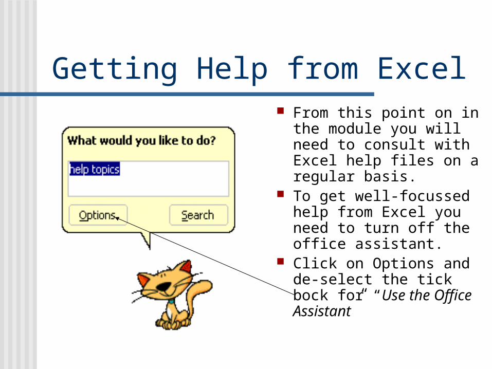
Getting Help from Excel From this point on in

the module you will need to consult with Excel help files on a regular basis.

To get well-focussed help from Excel you need to turn off the office assistant.

Click on Options and de-select the tick bock for “Use the Office Assistant”

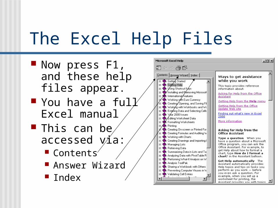
The Excel Help Files Now press F1, and

these help files appear.

You have a full Excel manual

This can be accessed via: Contents Answer Wizard Index

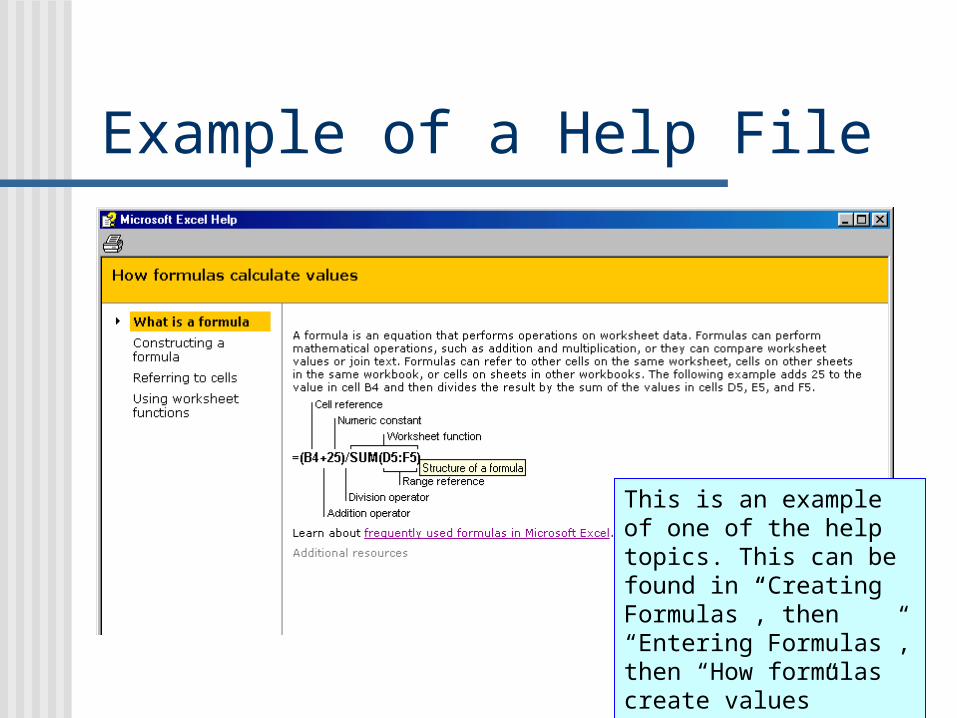
Example of a Help File

This is an example of one of the help topics. This can be found in “Creating Formulas”, then “Entering Formulas”, then “How formulas create values”

Functions in Excel A function can be

thought of as a tool for doing a specific task.

For example, instead of typing in a string of additions: A1+A2+A3+A4,

we can use the SUM function: SUM(A1:A4)

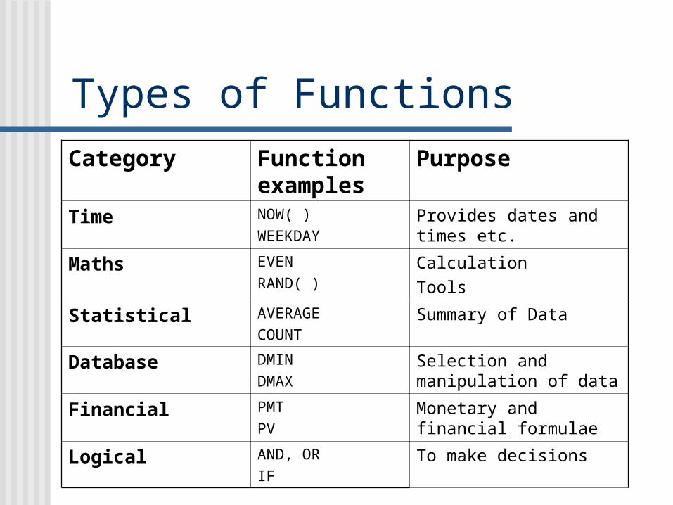
Types of FunctionsCategory Function

examplesPurpose

Time NOW( )WEEKDAY

Provides dates and times etc.

Maths EVENRAND( )

CalculationTools

Statistical AVERAGECOUNT

Summary of Data

Database DMINDMAX

Selection and manipulation of data

Financial PMTPV

Monetary and financial formulae

Logical AND, ORIF

To make decisions

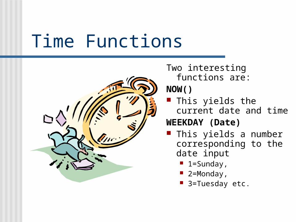
Time FunctionsTwo interesting functions

are:NOW() This yields the current

date and timeWEEKDAY (Date) This yields a number

corresponding to the date input 1=Sunday, 2=Monday, 3=Tuesday etc.

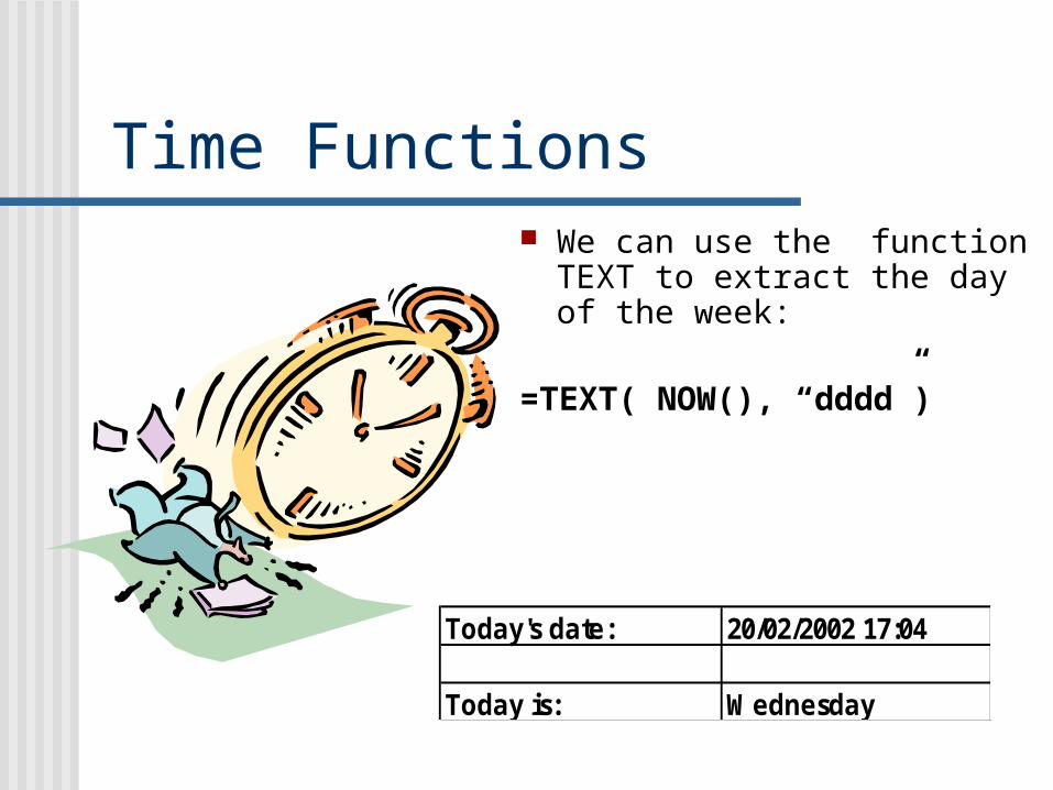
Time Functions We can use the function

TEXT to extract the day of the week:

=TEXT( NOW(), “dddd”)

Today's date: 20/02/2002 17:04

Today is: Wednesday

Time Functions There are many

more functions to investigate

Try looking up: DATEDIF WORKDAYS YEARFRAC

Arithmetic Functions There are two functions for dealing with

decimals:TRUNC

This truncates a number at the decimal point, removing the fractional part.

ROUND This rounds a number, either rounding up or

rounding down, according to convention The format is

ROUND( value, number of dec. places required)

Arithmetic Functions

Examples: suppose A5 contains the number

3.262TRUNC

TRUNC(A5) yields the answer 3.

ROUND ROUND(A5, 1) gives the answer 3.3 ROUND(A5, 2) gives the answer 3.26

Arithmetic FunctionsFunctions related to division:QUOTIENT This gives the whole number

part of the answer when one number is divided by another.

MOD This gives the remainder

when one number is divided by another

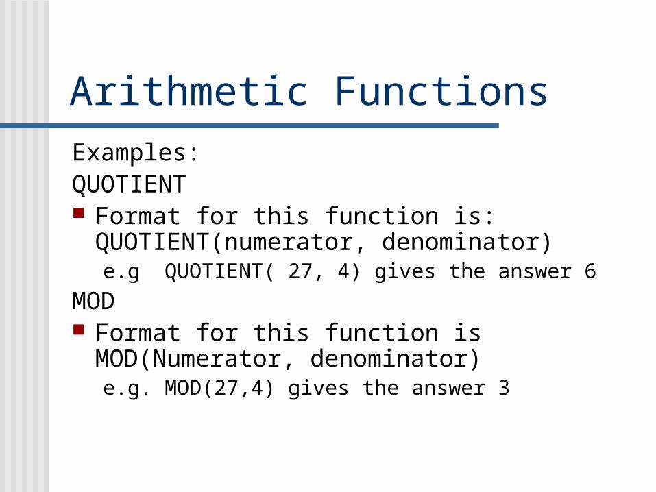
Arithmetic FunctionsExamples:QUOTIENT Format for this function is:

QUOTIENT(numerator, denominator)e.g QUOTIENT( 27, 4) gives the answer 6

MOD Format for this function is MOD(Numerator,

denominator)e.g. MOD(27,4) gives the answer 3

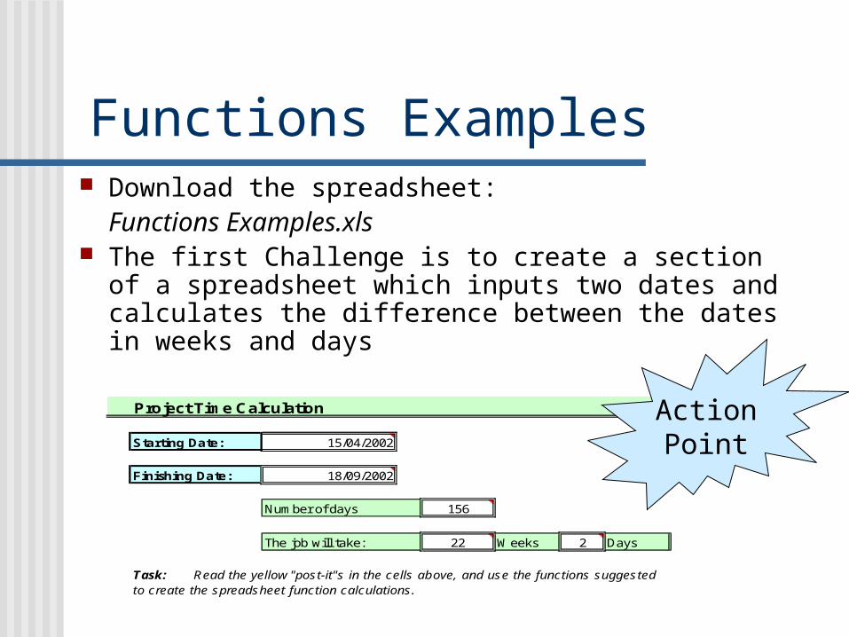
Functions Examples Download the spreadsheet:

Functions Examples.xls The first Challenge is to create a section of a

spreadsheet which inputs two dates and calculates the difference between the dates in weeks and days

Project Time Calculation

Starting Date: 15/04/2002

Finishing Date: 18/09/2002

Number of days 156

The job will take: 22 Weeks 2 Days

Task: Read the yellow "post-it"s in the cells above, and use the functions suggested to create the spreadsheet function calculations.

ActionPoint

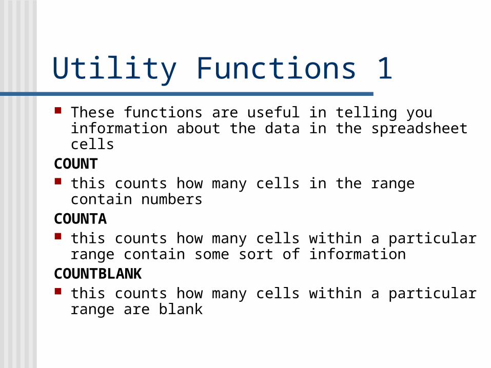
Utility Functions 1 These functions are useful in telling you

information about the data in the spreadsheet cellsCOUNT this counts how many cells in the range contain

numbersCOUNTA this counts how many cells within a particular

range contain some sort of informationCOUNTBLANK this counts how many cells within a particular

range are blank

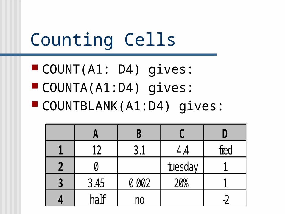
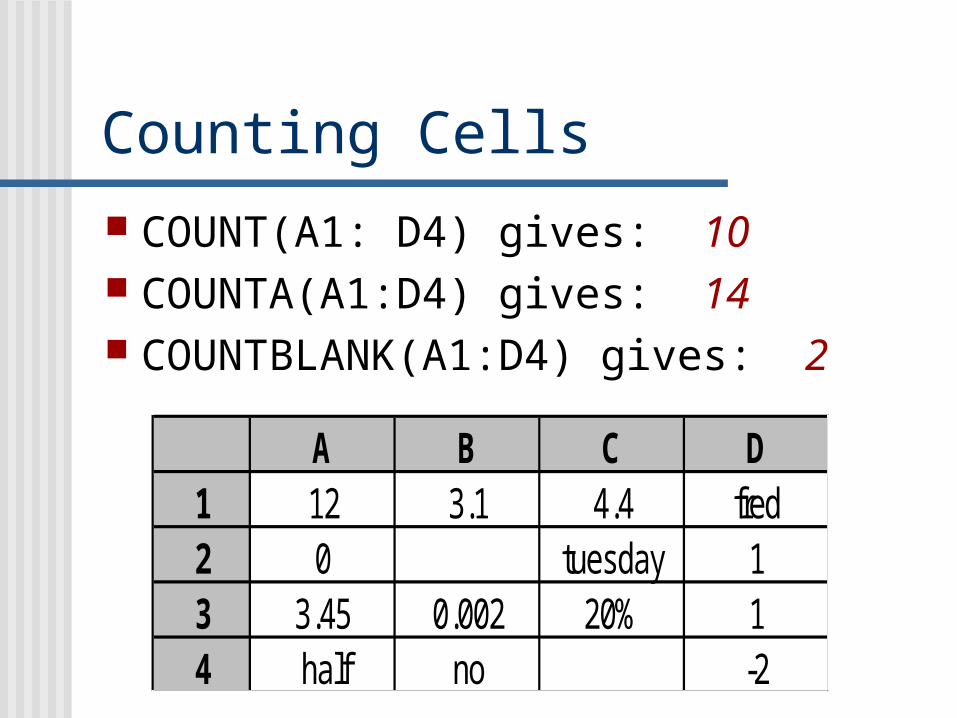
Counting Cells

A B C D1 12 3.1 4.4 fred2 0 tuesday 13 3.45 0.002 20% 14 half no -2

COUNT(A1: D4) gives: COUNTA(A1:D4) gives: COUNTBLANK(A1:D4) gives:

Counting Cells

A B C D1 12 3.1 4.4 fred2 0 tuesday 13 3.45 0.002 20% 14 half no -2

COUNT(A1: D4) gives: 10 COUNTA(A1:D4) gives: 14 COUNTBLANK(A1:D4) gives: 2

Utility Functions 2 These functions are useful in telling you

information about the data in specific spreadsheet cells.

They return TRUE or FALSEISBLANK tells you whether a specific cell is emptyISNUMBER tells you whether a specific cell contains a

numerical entryISTEXT Tells you whether a particular cell contains text

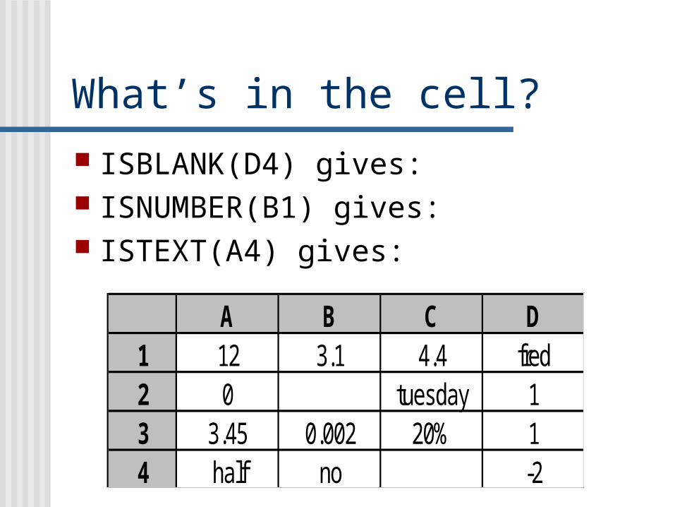
What’s in the cell? ISBLANK(D4) gives: ISNUMBER(B1) gives: ISTEXT(A4) gives:

A B C D1 12 3.1 4.4 fred2 0 tuesday 13 3.45 0.002 20% 14 half no -2

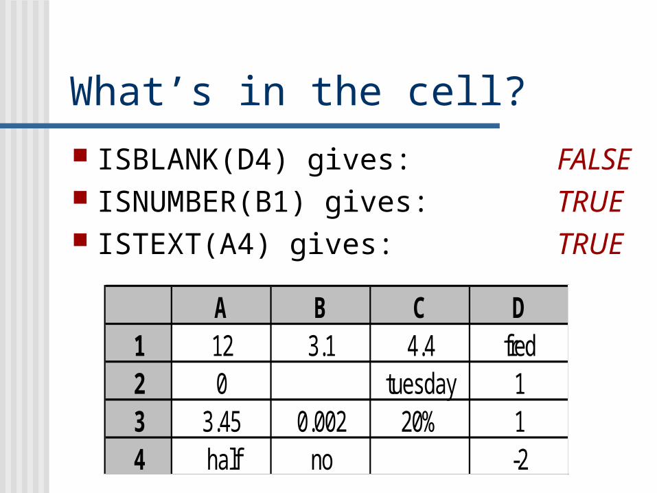
What’s in the cell? ISBLANK(D4) gives: FALSE ISNUMBER(B1) gives: TRUE ISTEXT(A4) gives: TRUE

A B C D1 12 3.1 4.4 fred2 0 tuesday 13 3.45 0.002 20% 14 half no -2

Functions Examples

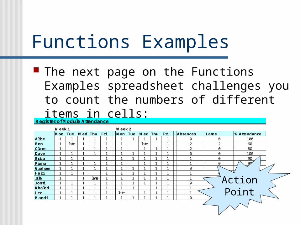
Register of Module Attendance

Week 1 Week 2Mon Tue Wed Thu Fri Mon Tue Wed Thu Fri Absences Lates % Attendance

Alice 1 1 1 1 1 1 1 1 1 1 0 0 100Ben 1 late 1 1 1 1 late 1 2 2 60Clare 1 1 1 1 1 1 1 1 2 0 80Dave 1 1 1 1 1 1 1 1 1 1 0 0 100Erica 1 1 1 1 1 1 1 1 1 1 0 90Fiona 1 1 1 1 1 1 1 1 1 1 0 90Graham 1 1 1 1 1 1 1 1 1 1 0 0 100Hajii 1 1 1 1 1 1 1 1 1 1 0 90Isla 1 1 late 1 1 1 1 1 1 1 1 80Jonti 1 1 1 1 1 1 1 1 1 1 0 0 100Khaled 1 1 1 1 1 1 1 1 1 1 0 90Lee 1 1 1 1 1 late 1 1 1 1 1 80Mandi 1 1 1 1 1 1 1 1 1 1 0 0 100

The next page on the Functions Examples spreadsheet challenges you to count the numbers of different items in cells:

ActionPoint

Look Up Tables Look Up Tables are one

of the most useful features of Excel.

These tables allow you to select from of a list of options using a particular value as a reference

The simplest of the functions is LOOKUP

LOOKUP(cell, range)

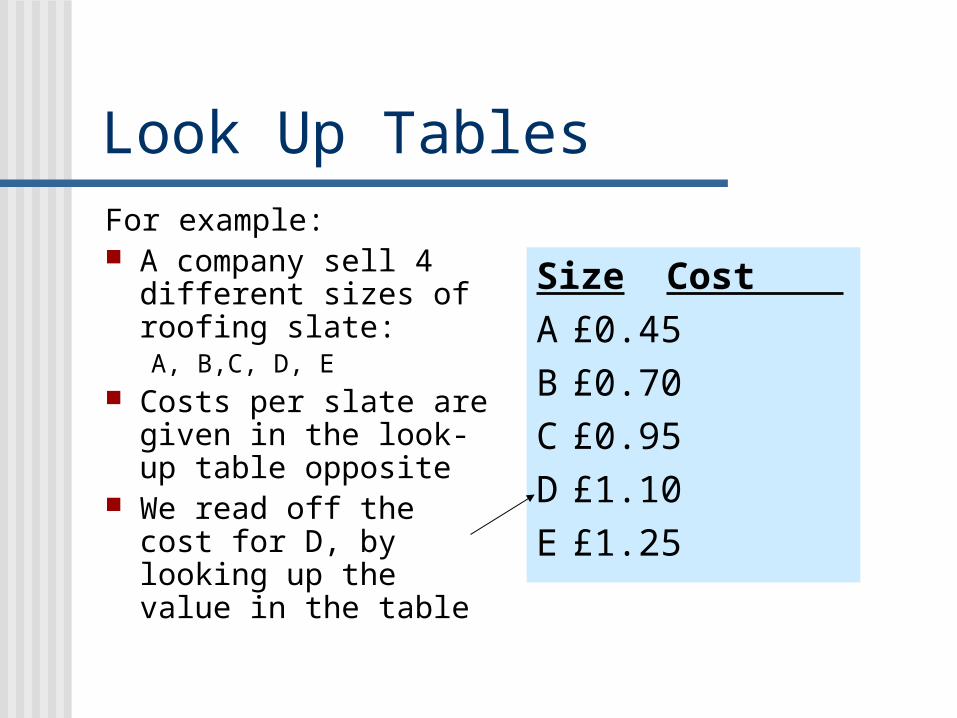
Look Up TablesFor example: A company sell 4

different sizes of roofing slate: A, B,C, D, E

Costs per slate are given in the look-up table opposite

We read off the cost for D, by looking up the value in the table

Size Cost

A £0.45B £0.70C £0.95D £1.10E £1.25

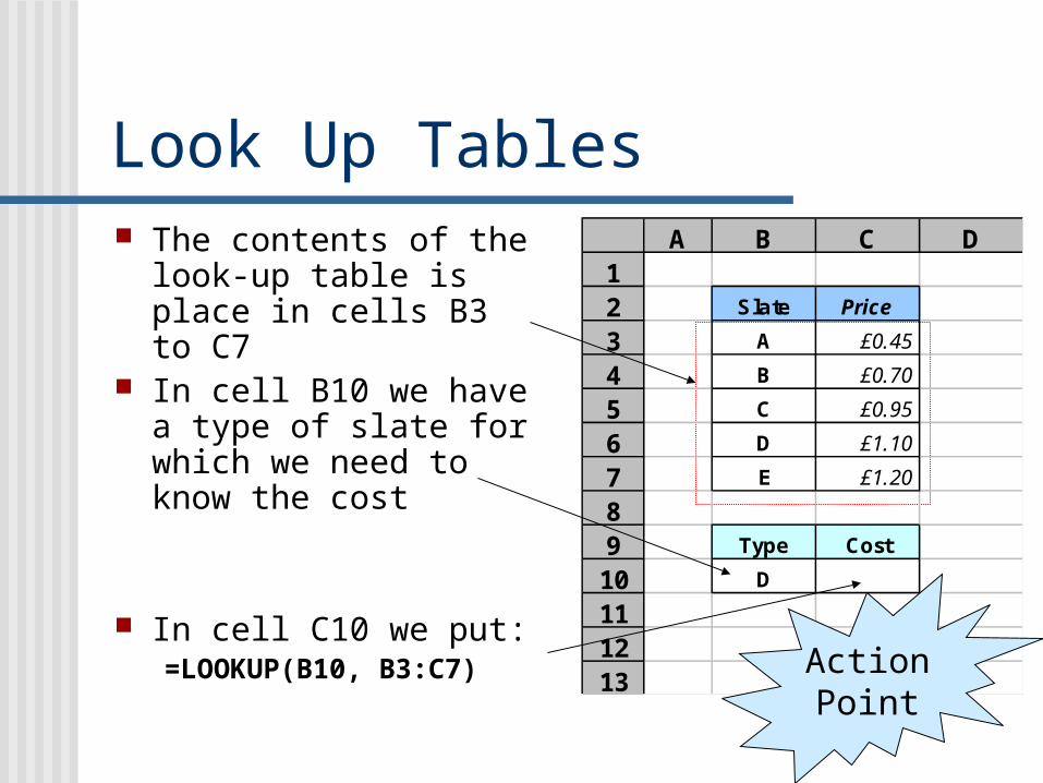
Look Up Tables The contents of the

look-up table is place in cells B3 to C7

In cell B10 we have a type of slate for which we need to know the cost

In cell C10 we put:=LOOKUP(B10, B3:C7)

A B C D12 Slate Price

3 A £0.45

4 B £0.70

5 C £0.95

6 D £1.10

7 E £1.20

89 Type Cost

10 D

111213 Action

Point

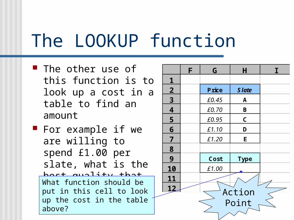
The LOOKUP function The other use of this

function is to look up a cost in a table to find an amount

For example if we are willing to spend £1.00 per slate, what is the best quality that we can afford?

F G H I12 Price Slate

3 £0.45 A

4 £0.70 B

5 £0.95 C

6 £1.10 D

7 £1.20 E

89 Cost Type

10 £1.00

1112

What function should be put in this cell to look up the cost in the table above?

ActionPoint

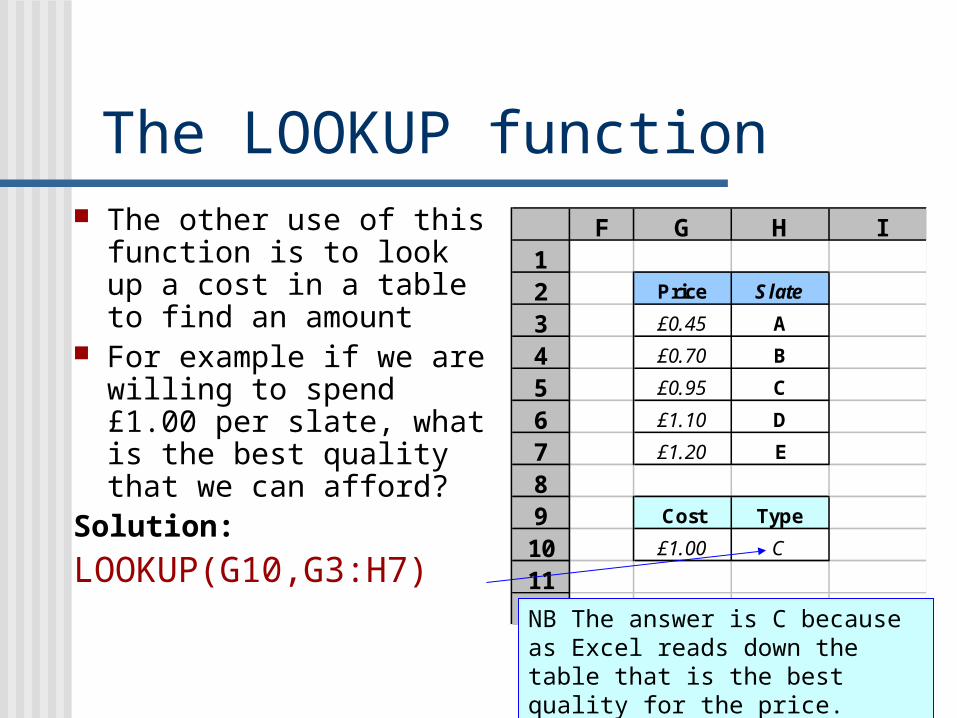
The LOOKUP function The other use of this

function is to look up a cost in a table to find an amount

For example if we are willing to spend £1.00 per slate, what is the best quality that we can afford?

Solution:

LOOKUP(G10,G3:H7)

F G H I12 Price Slate

3 £0.45 A

4 £0.70 B

5 £0.95 C

6 £1.10 D

7 £1.20 E

89 Cost Type

10 £1.00 C

1112NB The answer is C because as Excel reads down the table that is the best quality for the price.

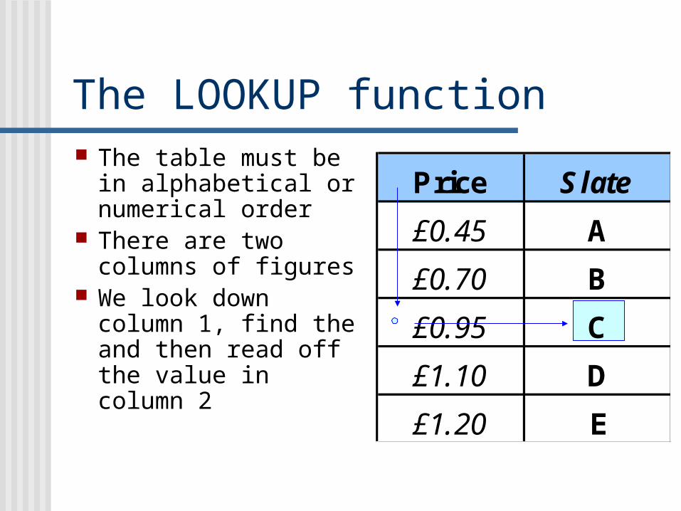
The LOOKUP function The table must be

in alphabetical or numerical order

There are two columns of figures

We look down column 1, find the and then read off the value in column 2

Price Slate

£0.45 A

£0.70 B

£0.95 C

£1.10 D

£1.20 E

VLOOKUP VLOOKUP is an

extension of the idea, allowing you to create blocks of cells which contain different lookup values for different circumstances

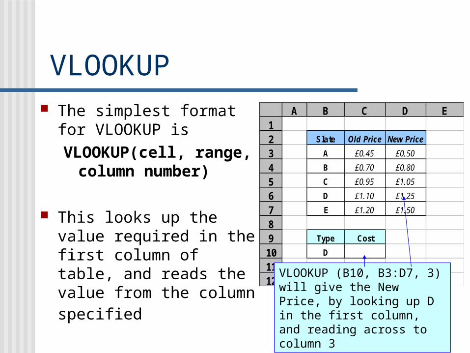
VLOOKUP The simplest format for

VLOOKUP isVLOOKUP(cell, range,

column number)

This looks up the value required in the first column of table, and reads the value from the column specified

A B C D E12 Slate Old Price New Price

3 A £0.45 £0.50

4 B £0.70 £0.80

5 C £0.95 £1.05

6 D £1.10 £1.25

7 E £1.20 £1.50

89 Type Cost

10 D

1112

VLOOKUP (B10, B3:D7, 3) will give the New Price, by looking up D in the first column, and reading across to column 3

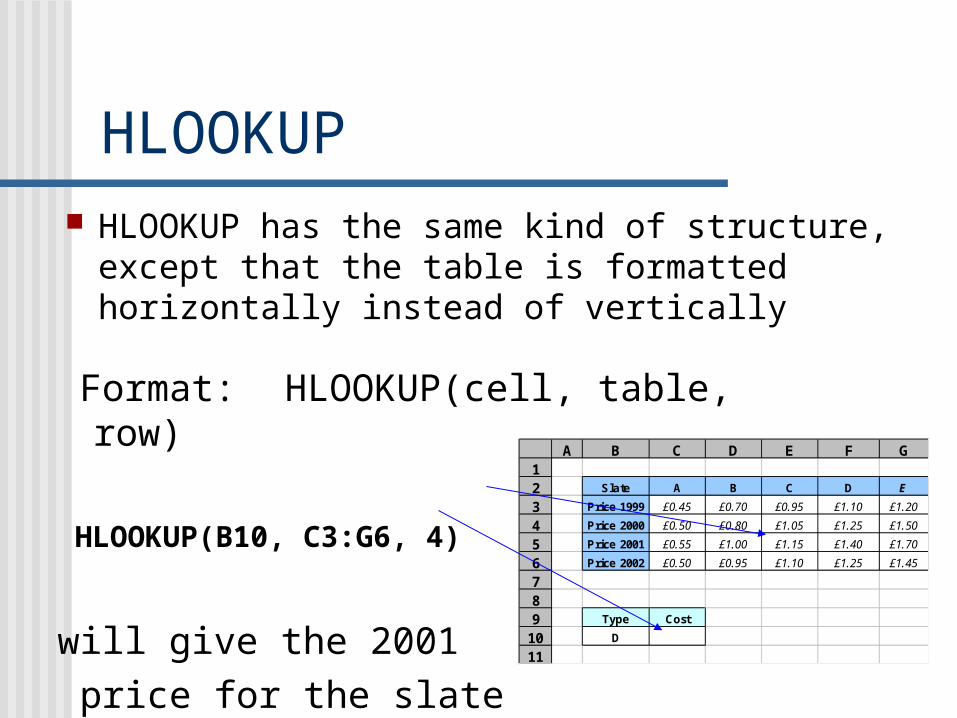
HLOOKUP HLOOKUP has the same kind of structure,

except that the table is formatted horizontally instead of vertically

A B C D E F G12 Slate A B C D E

3 Price 1999 £0.45 £0.70 £0.95 £1.10 £1.20

4 Price 2000 £0.50 £0.80 £1.05 £1.25 £1.50

5 Price 2001 £0.55 £1.00 £1.15 £1.40 £1.70

6 Price 2002 £0.50 £0.95 £1.10 £1.25 £1.45

789 Type Cost

10 D

11

Format: HLOOKUP(cell, table, row)

HLOOKUP(B10, C3:G6, 4)

will give the 2001 price for the slate

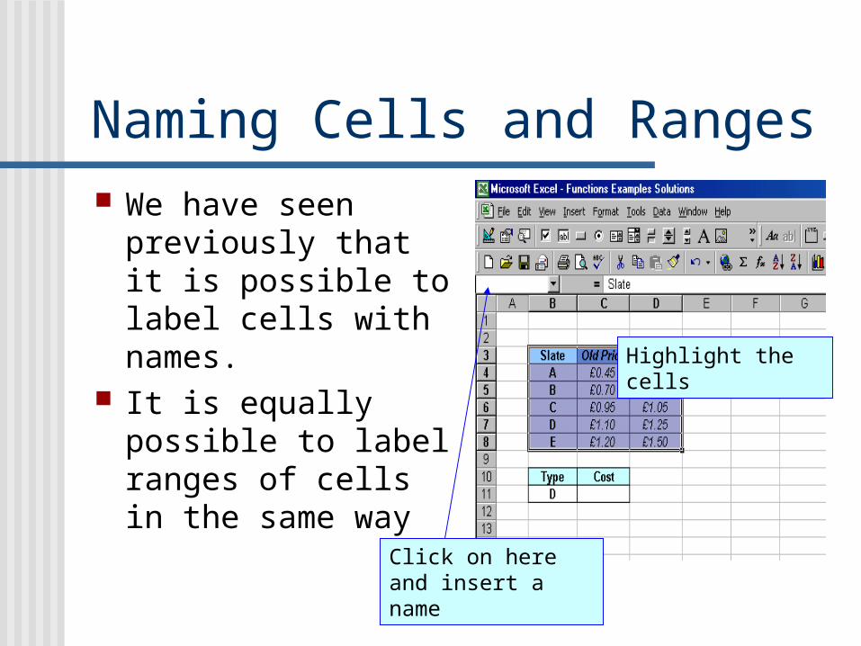
Naming Cells and Ranges We have seen

previously that it is possible to label cells with names.

It is equally possible to label ranges of cells in the same way

Highlight the cells

Click on here and insert a name

Using Name Ranges in Formulae

Slate Old Price New PriceA £0.45 £0.50B £0.70 £0.80C £0.95 £1.05D £1.10 £1.25E £1.20 £1.50

Type CostD

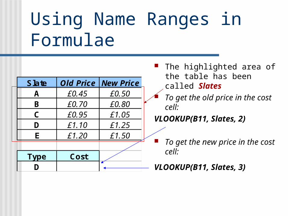
The highlighted area of the table has been called Slates

To get the old price in the cost cell:

VLOOKUP(B11, Slates, 2)

To get the new price in the cost cell:

VLOOKUP(B11, Slates, 3)

Functions Examples

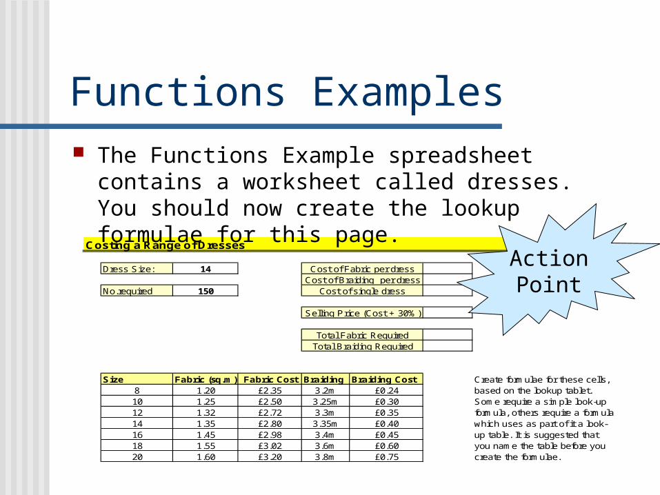
Costing a Range of Dresses

Dress Size: 14

No.required 150

Size Fabric (sq.m) Fabric Cost Braiding Braiding Cost8 1.20 £2.35 3.2m £0.2410 1.25 £2.50 3.25m £0.3012 1.32 £2.72 3.3m £0.3514 1.35 £2.80 3.35m £0.4016 1.45 £2.98 3.4m £0.4518 1.55 £3.02 3.6m £0.6020 1.60 £3.20 3.8m £0.75

Cost of Fabric per dressCost of Braiding per dress

Total Fabric RequiredTotal Braiding Required

Selling Price (Cost + 30%)

Cost of single dress

Create formulae for these cells, based on the lookup tablet. Some require a simple look-up formula, others require a formula which uses as part of it a look-up table. It is suggested that you name the table before you create the formulae.

The Functions Example spreadsheet contains a worksheet called dresses. You should now create the lookup formulae for this page.

ActionPoint

Other Table FunctionsMATCH This looks for a specific value in a single

column or row, and returns a number that indicates the position in an ordered list.

e.g MATCH( D5, D1:D10) returns the position that D5 would have if the set of values D1 to D10 were placed in ascending order

If the matching is done with text, MATCH yields the position of the text in the list.

MATCH

A B C12 Price Goods

3 £7.99 Shirt

4 £4.50 Tie

5 £24.99 Trousers

6 £5.45 Socks

7 £18.99 Shoes

8

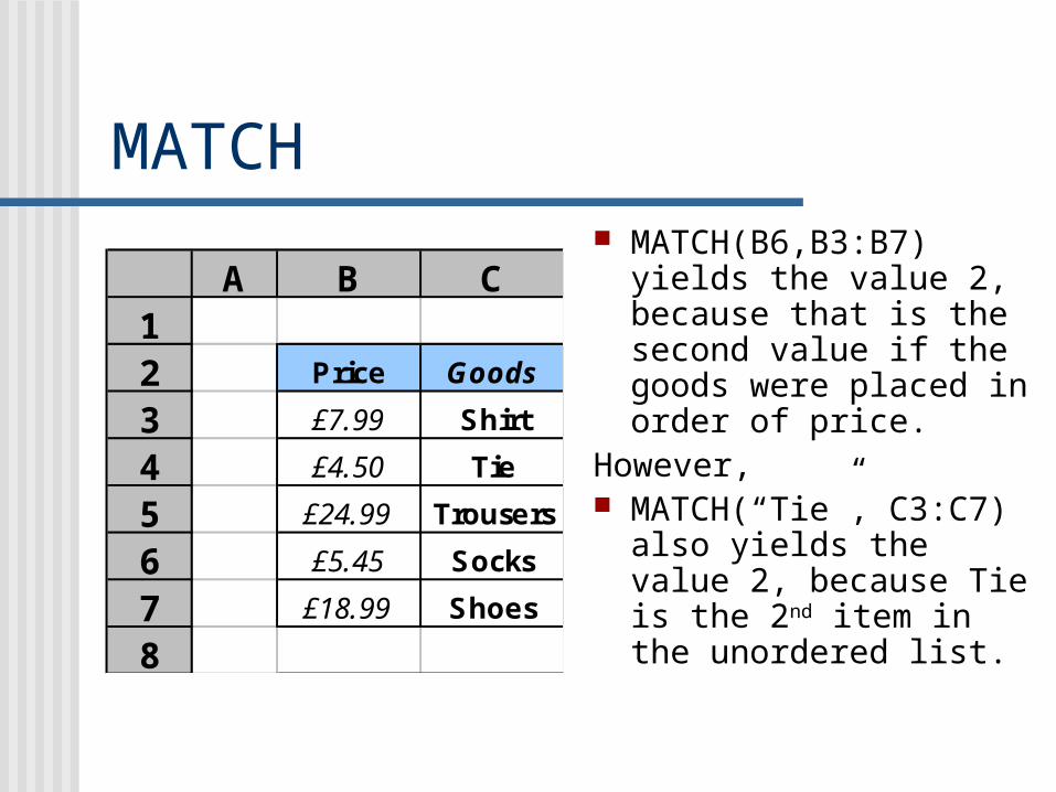
MATCH(B6,B3:B7) yields the value 2, because that is the second value if the goods were placed in order of price.

However, MATCH(“Tie”, C3:C7)

also yields the value 2, because Tie is the 2nd item in the unordered list.

Other Table Functions

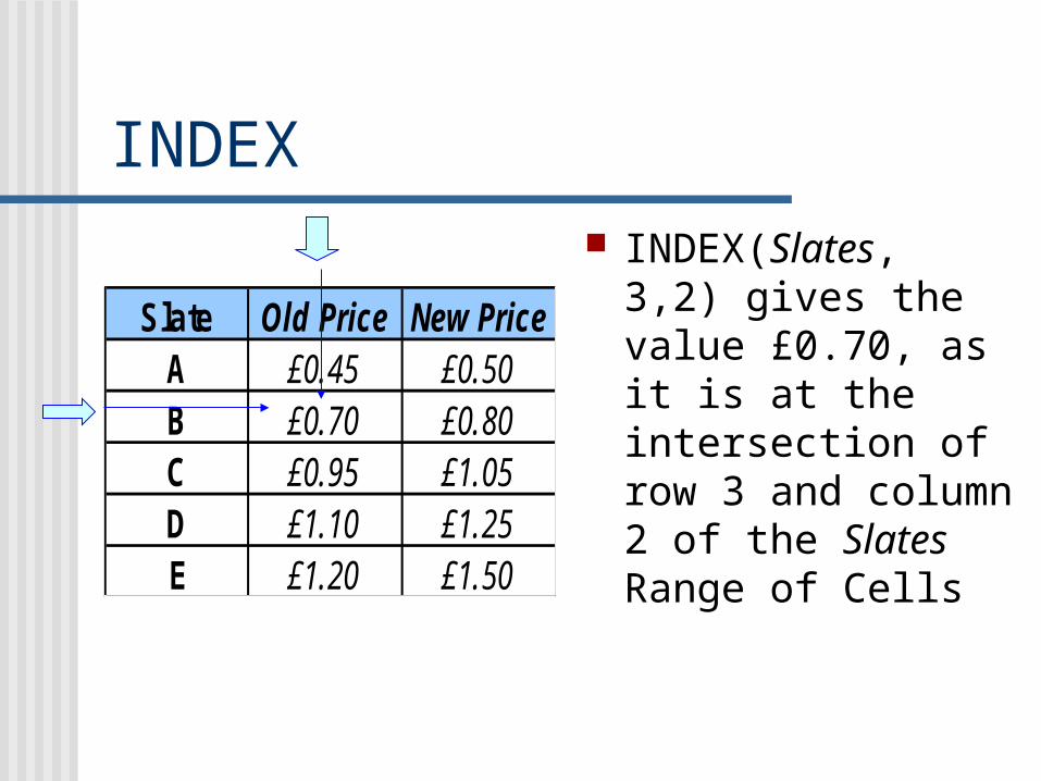
INDEX This function returns the value of a

cell which is located within a named range of cells

INDEX(range, row, column) gives the contents of a particular cell at the intersection of the row and column of a block of cells

INDEX

Slate Old Price New PriceA £0.45 £0.50B £0.70 £0.80C £0.95 £1.05D £1.10 £1.25E £1.20 £1.50

INDEX(Slates, 3,2) gives the value £0.70, as it is at the intersection of row 3 and column 2 of the Slates Range of Cells

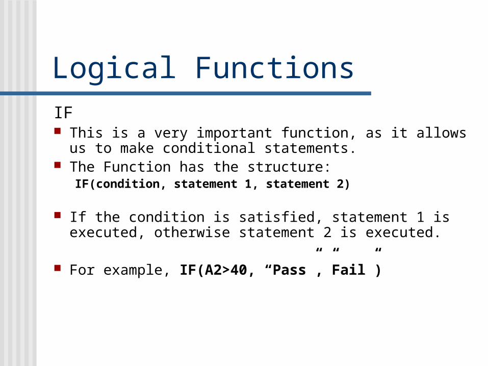
Logical FunctionsIF This is a very important function, as it allows us to

make conditional statements. The Function has the structure:

IF(condition, statement 1, statement 2)

If the condition is satisfied, statement 1 is executed, otherwise statement 2 is executed.

For example, IF(A2>40, “Pass”,”Fail”)

Logical Functions

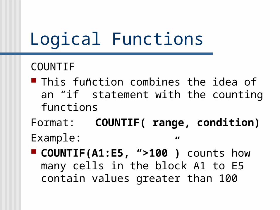
COUNTIF This function combines the idea of an “if”

statement with the counting functionsFormat: COUNTIF( range, condition)Example: COUNTIF(A1:E5, “>100”) counts how

many cells in the block A1 to E5 contain values greater than 100

Functions Examples

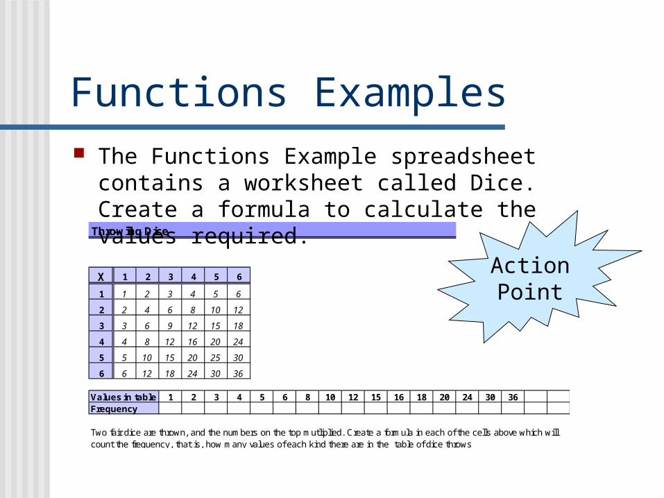
Throwing Dice

X 1 2 3 4 5 6

1 1 2 3 4 5 6

2 2 4 6 8 10 12

3 3 6 9 12 15 18

4 4 8 12 16 20 24

5 5 10 15 20 25 30

6 6 12 18 24 30 36

Values in table 1 2 3 4 5 6 8 10 12 15 16 18 20 24 30 36Frequency

Two fair dice are thrown, and the numbers on the top mutliplied. Create a formula in each of the cells above which will count the frequency, that is, how many values of each kind there are in the table of dice throws

The Functions Example spreadsheet contains a worksheet called Dice. Create a formula to calculate the values required.

ActionPoint

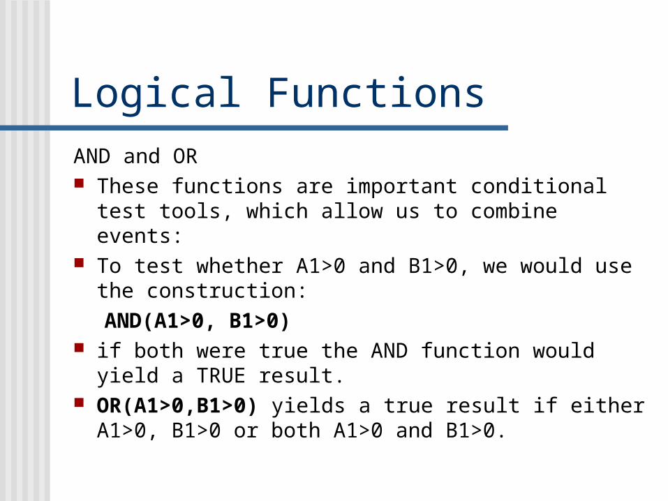
Logical FunctionsAND and OR These functions are important conditional test

tools, which allow us to combine events: To test whether A1>0 and B1>0, we would use

the construction:AND(A1>0, B1>0)

if both were true the AND function would yield a TRUE result.

OR(A1>0,B1>0) yields a true result if either A1>0, B1>0 or both A1>0 and B1>0.

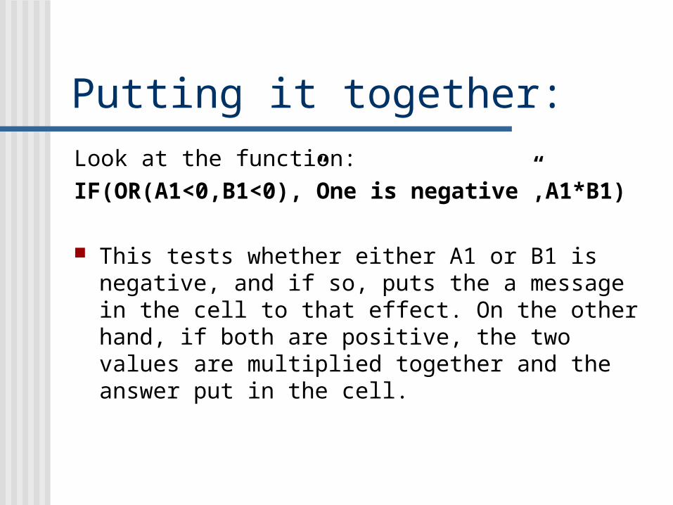
Putting it together:Look at the function:IF(OR(A1<0,B1<0),”One is negative”,A1*B1)

This tests whether either A1 or B1 is negative, and if so, puts the a message in the cell to that effect. On the other hand, if both are positive, the two values are multiplied together and the answer put in the cell.

Functions Examples

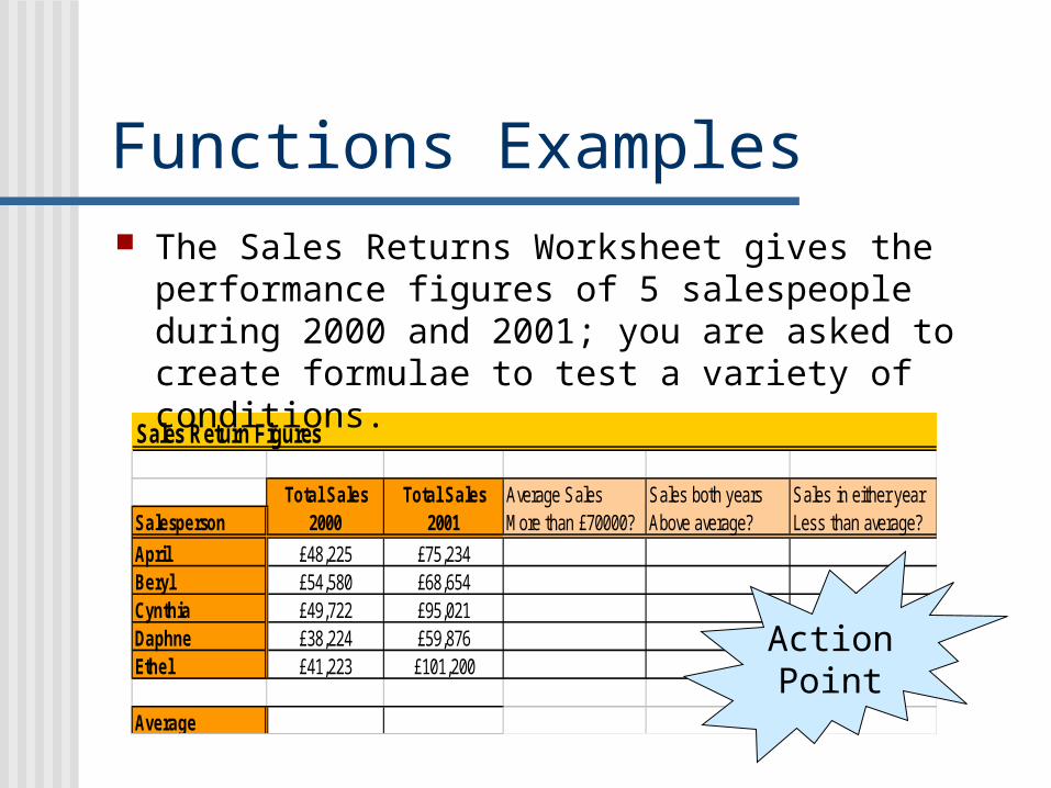
Sales Return Figures

Total Sales Total Sales Average Sales Sales both years Sales in either year Salesperson 2000 2001 More than £70000? Above average? Less than average?

April £48,225 £75,234Beryl £54,580 £68,654Cynthia £49,722 £95,021Daphne £38,224 £59,876Ethel £41,223 £101,200

Average

The Sales Returns Worksheet gives the performance figures of 5 salespeople during 2000 and 2001; you are asked to create formulae to test a variety of conditions.

ActionPoint

Text Functions

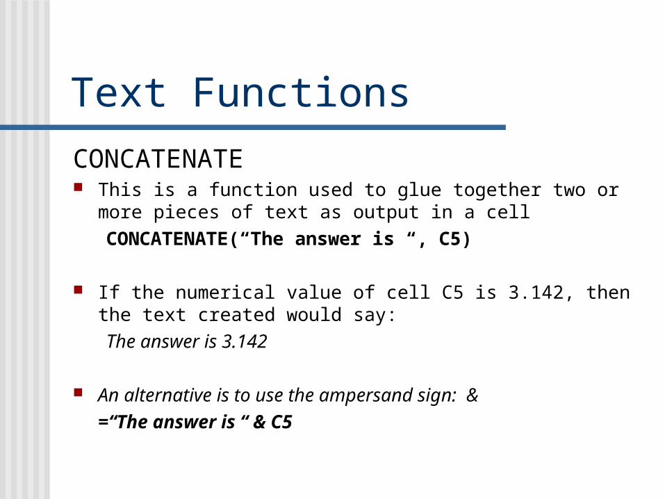
CONCATENATE This is a function used to glue together two or more pieces

of text as output in a cellCONCATENATE(“The answer is “, C5)

If the numerical value of cell C5 is 3.142, then the text created would say: The answer is 3.142

An alternative is to use the ampersand sign: &=“The answer is “ & C5

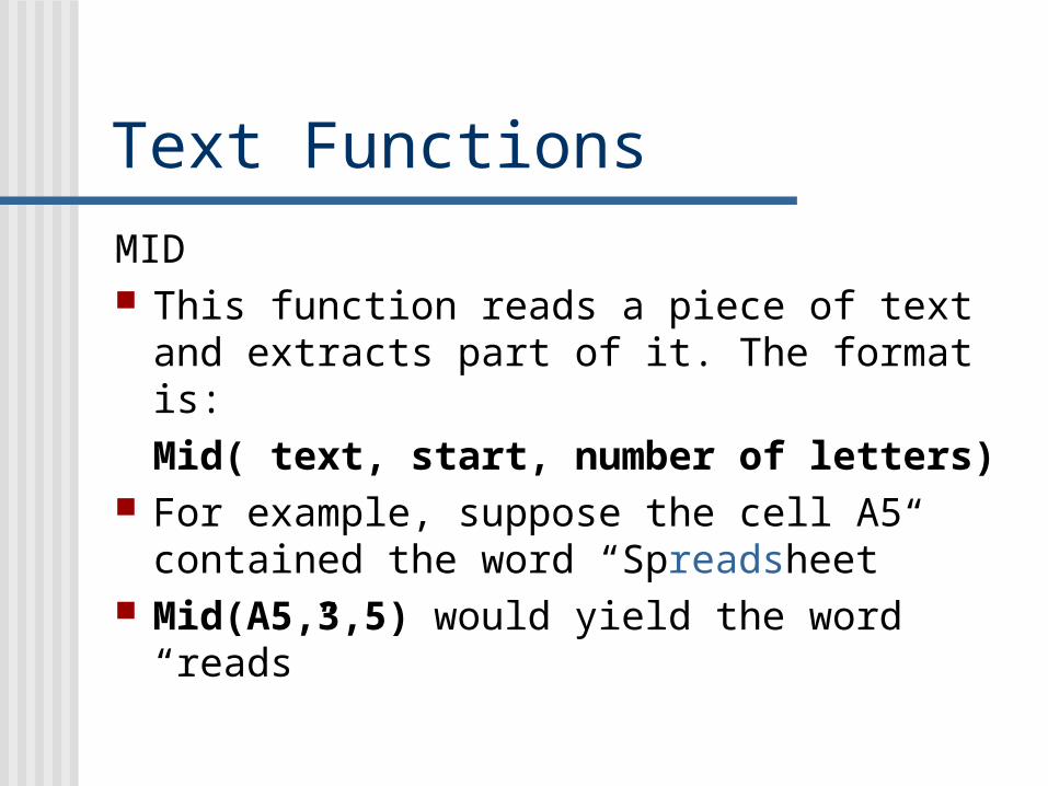
Text Functions

MID This function reads a piece of text and

extracts part of it. The format is:Mid( text, start, number of letters)

For example, suppose the cell A5 contained the word “Spreadsheet”

Mid(A5,3,5) would yield the word “reads”

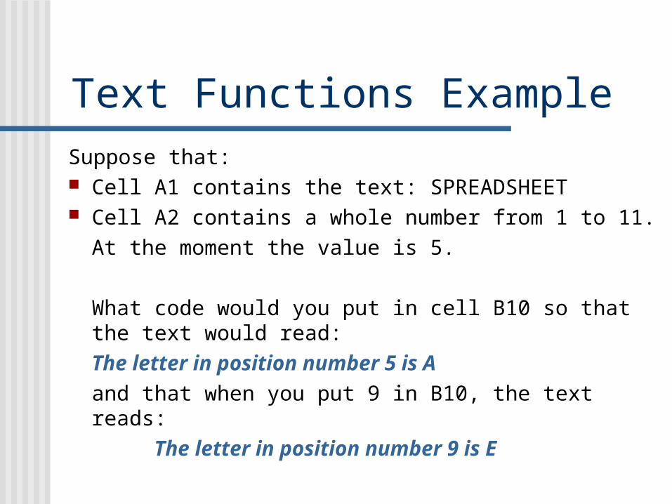
Text Functions ExampleSuppose that: Cell A1 contains the text: SPREADSHEET Cell A2 contains a whole number from 1 to 11.

At the moment the value is 5.

What code would you put in cell B10 so that the text would read:

The letter in position number 5 is Aand that when you put 9 in B10, the text reads: The letter in position number 9 is E

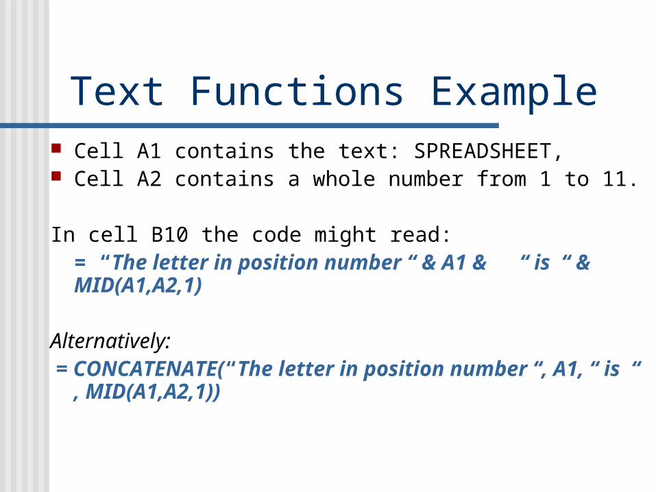
Text Functions Example Cell A1 contains the text: SPREADSHEET, Cell A2 contains a whole number from 1 to 11.

In cell B10 the code might read:= “The letter in position number “ & A1 & “ is “ & MID(A1,A2,1)

Alternatively: = CONCATENATE(“The letter in position

number “, A1, “ is “ , MID(A1,A2,1))

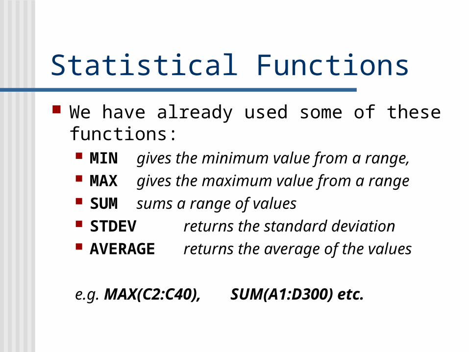
Statistical Functions We have already used some of these

functions: MIN gives the minimum value from a range, MAX gives the maximum value from a range SUM sums a range of values STDEV returns the standard deviation AVERAGE returns the average of the values

e.g. MAX(C2:C40), SUM(A1:D300) etc.

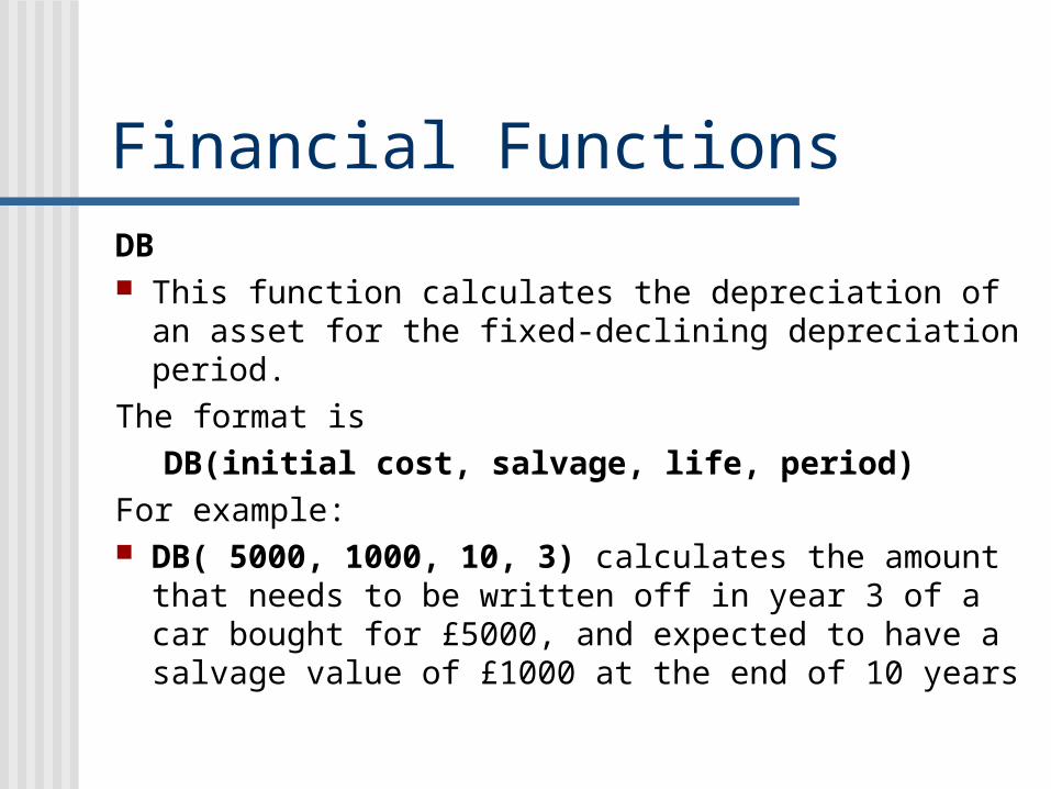
Financial FunctionsDB This function calculates the depreciation of an

asset for the fixed-declining depreciation period.The format is

DB(initial cost, salvage, life, period)For example: DB( 5000, 1000, 10, 3) calculates the amount

that needs to be written off in year 3 of a car bought for £5000, and expected to have a salvage value of £1000 at the end of 10 years

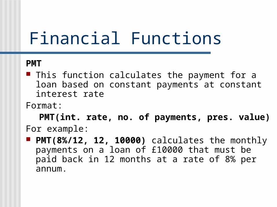
Financial FunctionsPMT This function calculates the payment for a loan

based on constant payments at constant interest rate

Format:PMT(int. rate, no. of payments, pres. value)

For example: PMT(8%/12, 12, 10000) calculates the monthly

payments on a loan of £10000 that must be paid back in 12 months at a rate of 8% per annum.

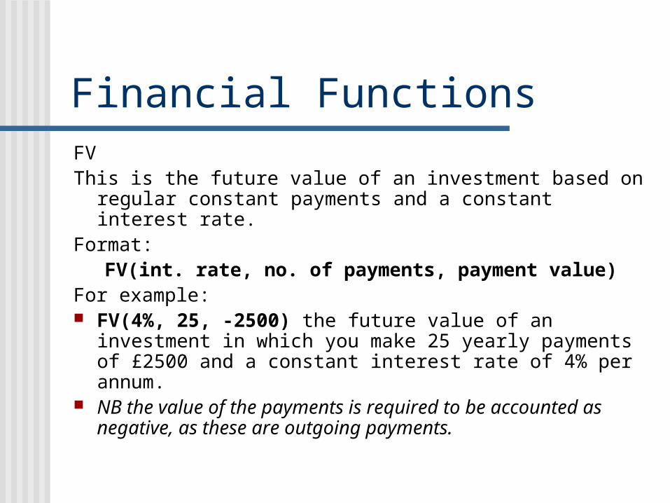
Financial FunctionsFVThis is the future value of an investment based on regular

constant payments and a constant interest rate.Format:

FV(int. rate, no. of payments, payment value)For example: FV(4%, 25, -2500) the future value of an investment

in which you make 25 yearly payments of £2500 and a constant interest rate of 4% per annum.

NB the value of the payments is required to be accounted as negative, as these are outgoing payments.

Functions Examples

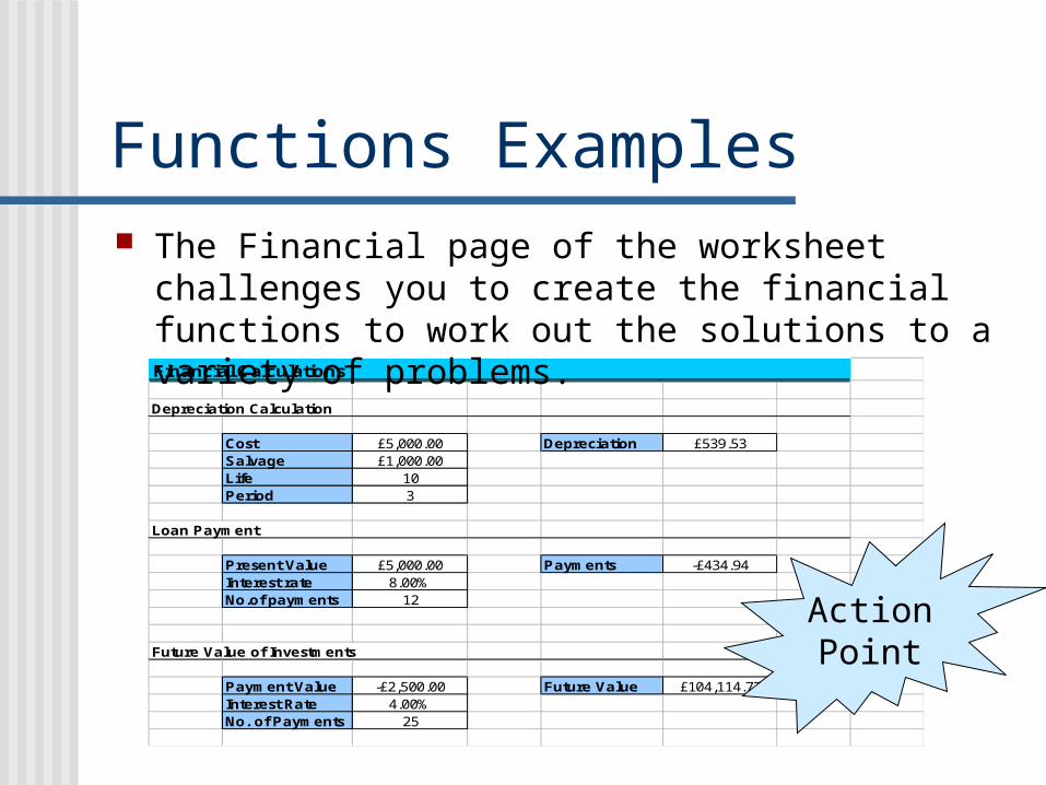
Financial Calculations

Depreciation Calculation

Cost £5,000.00 Depreciation £539.53Salvage £1,000.00Life 10Period 3

Loan Payment

Present Value £5,000.00 Payments -£434.94Interest rate 8.00%No.of payments 12

Future Value of Investments

Payment Value -£2,500.00 Future Value £104,114.77Interest Rate 4.00%No. of Payments 25

The Financial page of the worksheet challenges you to create the financial functions to work out the solutions to a variety of problems.

ActionPoint

More Functions Excel contains literally

hundreds of functions, some of which are quite similar to, and may of which are very different from the ones in this lecture.

In particular, as you look through the Excel help files, you will notice that we have been using only one form of these functions; each one has many variants.