Embed Size (px)
Citation preview
Spreadsheets in Finance and Forecasting
Week 4:Using Formulae
Working with Formulae In previous weeks we have seen that
we can work with cell formulae to calculate totals, averages and other summary values, and can keep running totals of transactions.
This week we explore this further, and look in depth at the processes behind formulae
Objectives for Week 4 After working through the materials
for this week you will be able to: Work confidently with spreadsheet
formulae Understand and work with operator
precedence Use absolute and relative addresses
and range names
Following the Slides When you see this You will need to open
the spreadsheets referred to in the slides
Switch between the slides and the spreadsheet to follow the examples
ActionPoint!
Flower Shop Example The next few
examples use Flower Sales.xls
This is a simple spreadsheet which carries out a number of calculations of sales and profits
ActionPoint!
Floral Arrangements
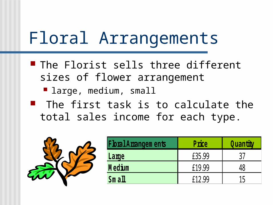
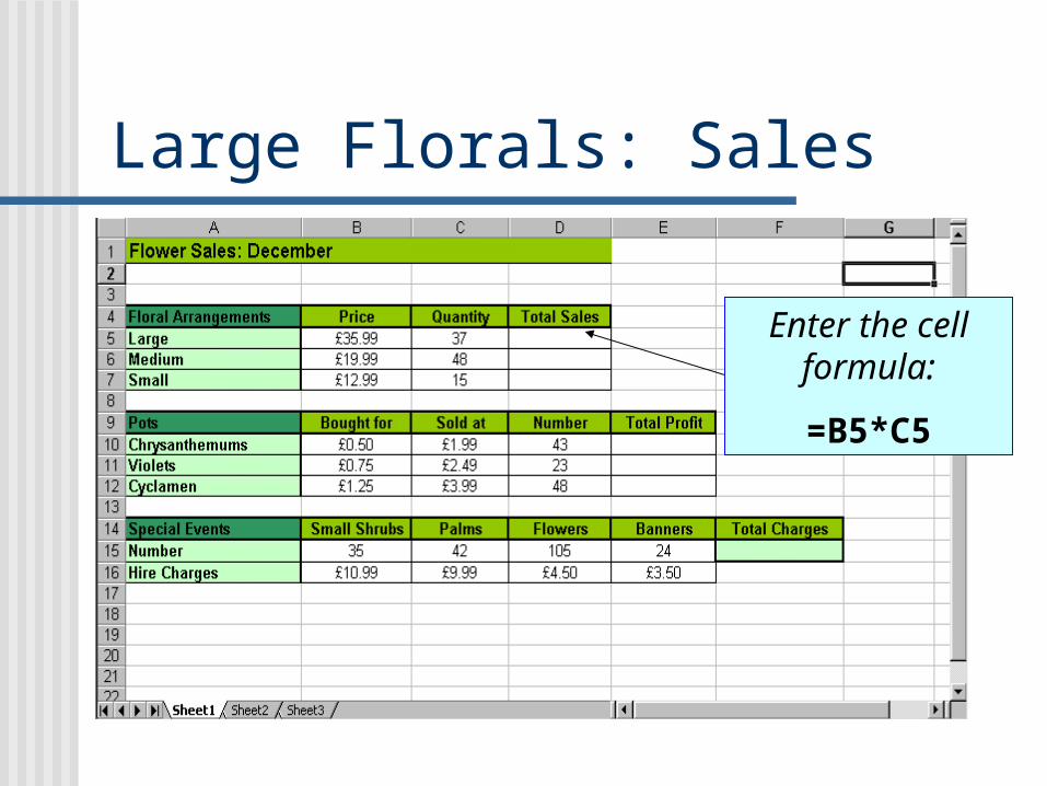
Floral Arrangements Price QuantityLarge £35.99 37Medium £19.99 48Small £12.99 15
The Florist sells three different sizes of flower arrangement large, medium, small
The first task is to calculate the total sales income for each type.
Large Florals: Sales
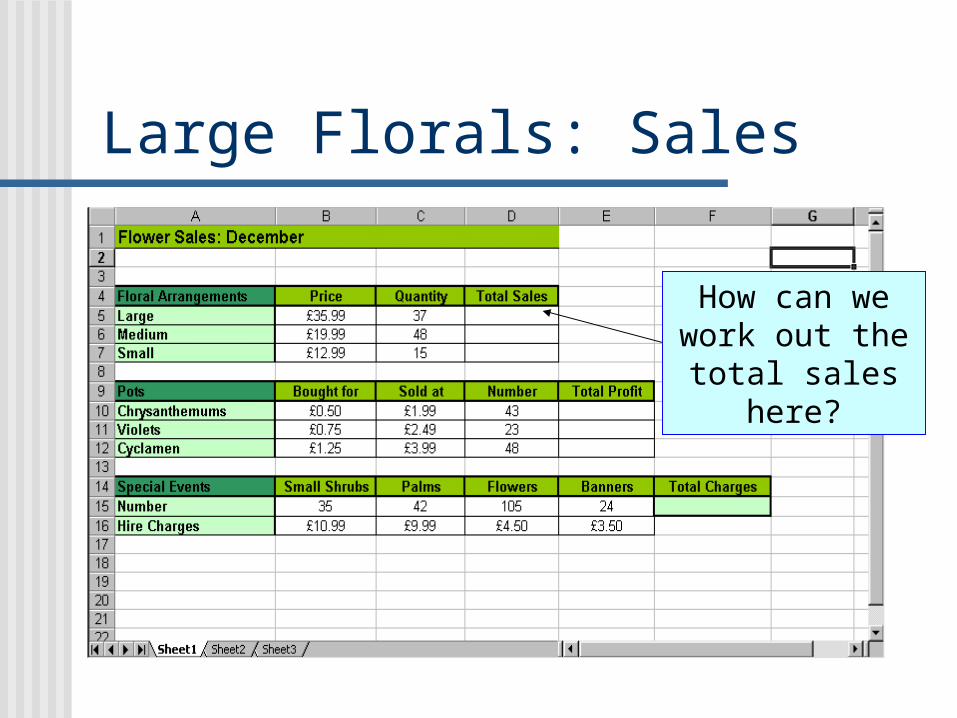
How can we work out the total sales
here?
Large Florals: Sales
Enter the cell formula:
=B5*C5
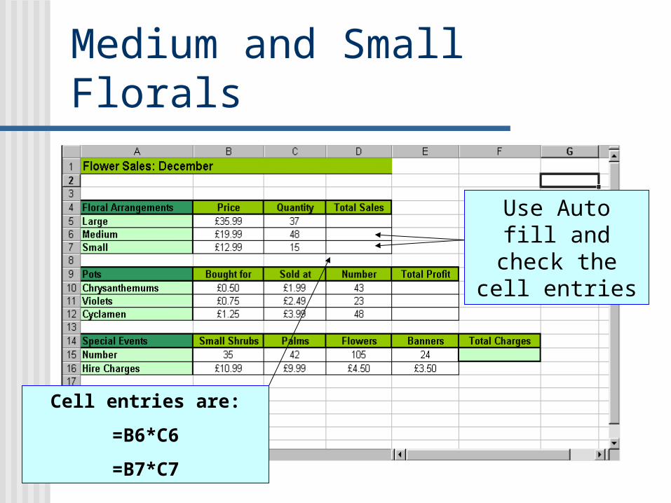
Medium and Small Florals
Use Auto fill and check the
cell entries
Cell entries are:
=B6*C6
=B7*C7
Pot Plants: Profits
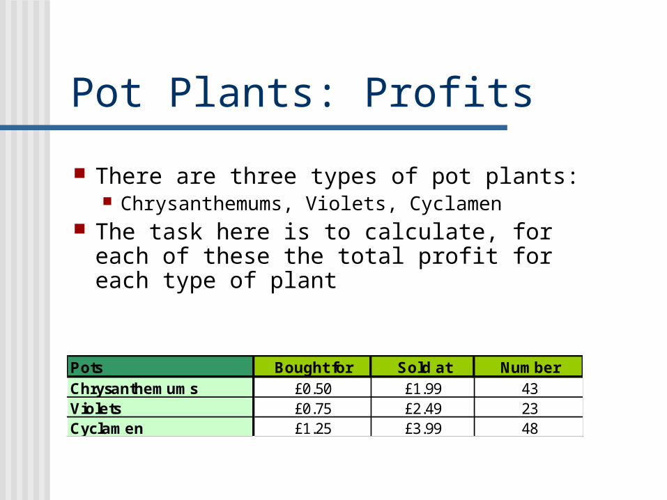
There are three types of pot plants: Chrysanthemums, Violets, Cyclamen
The task here is to calculate, for each of these the total profit for each type of plant
Pots Bought for Sold at NumberChrysanthemums £0.50 £1.99 43Violets £0.75 £2.49 23Cyclamen £1.25 £3.99 48
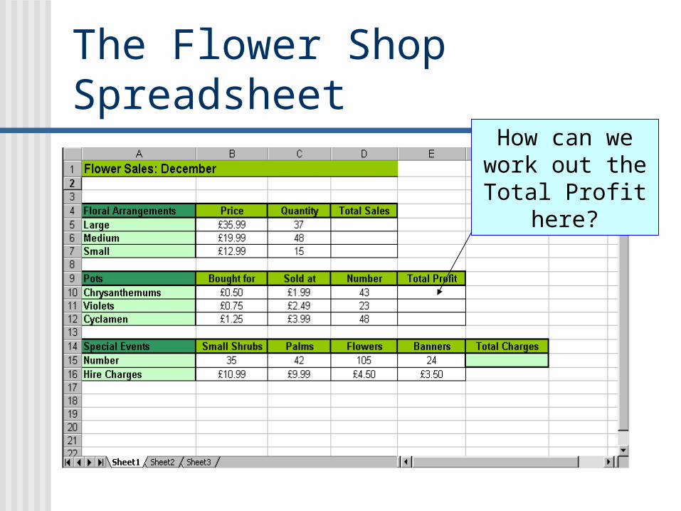
The Flower Shop Spreadsheet
How can we work out the Total Profit
here?
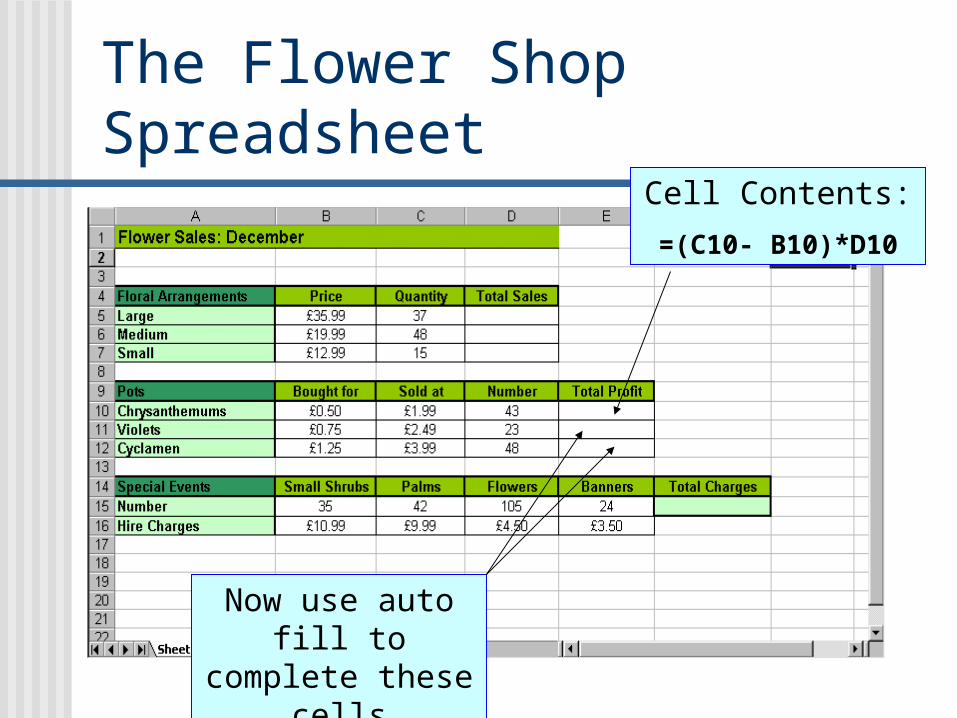
The Flower Shop Spreadsheet
Cell Contents:
=(C10- B10)*D10
Now use auto fill to complete these cells
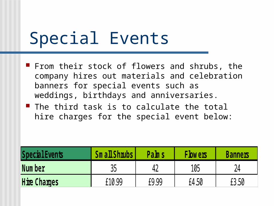
Special Events From their stock of flowers and shrubs, the
company hires out materials and celebration banners for special events such as weddings, birthdays and anniversaries.
The third task is to calculate the total hire charges for the special event below:
Special Events Small Shrubs Palms Flowers BannersNumber 35 42 105 24Hire Charges £10.99 £9.99 £4.50 £3.50
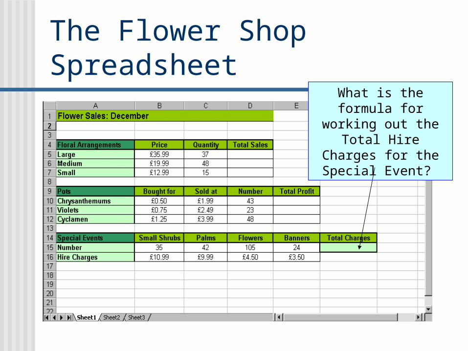
The Flower Shop Spreadsheet
What is the formula for working out the Total Hire Charges
for the Special Event?
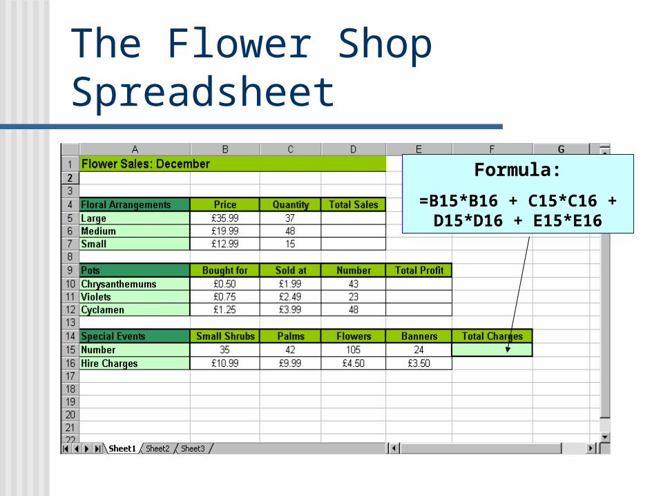
The Flower Shop Spreadsheet
Formula:
=B15*B16 + C15*C16 + D15*D16 + E15*E16

Operations In the previous
example we saw calculations being carried out on cell addresses using a formula
Such formulae rely on mathematical conventions
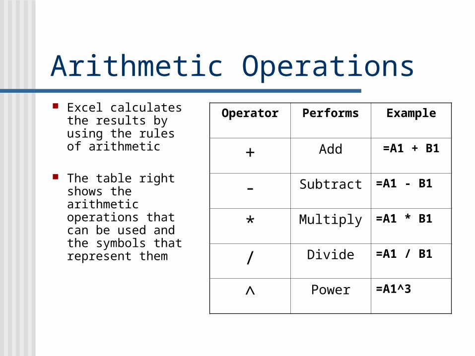
Arithmetic Operations Excel calculates the
results by using the rules of arithmetic
The table right shows the arithmetic operations that can be used and the symbols that represent them
Operator Performs Example
+ Add =A1 + B1
- Subtract =A1 - B1
* Multiply =A1 * B1
/ Divide =A1 / B1
^ Power =A1^3
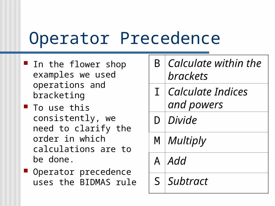
Operator Precedence In the flower shop
examples we used operations and bracketing
To use this consistently, we need to clarify the order in which calculations are to be done.
Operator precedence uses the BIDMAS rule
B Calculate within the brackets
I Calculate Indices and powers
D Divide
M Multiply
A Add
S Subtract
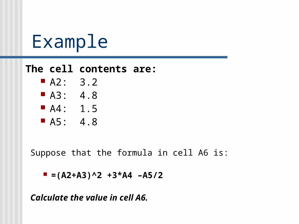
ExampleThe cell contents are:
A2: 3.2 A3: 4.8 A4: 1.5 A5: 4.8
Suppose that the formula in cell A6 is:
=(A2+A3)^2 +3*A4 –A5/2
Calculate the value in cell A6.
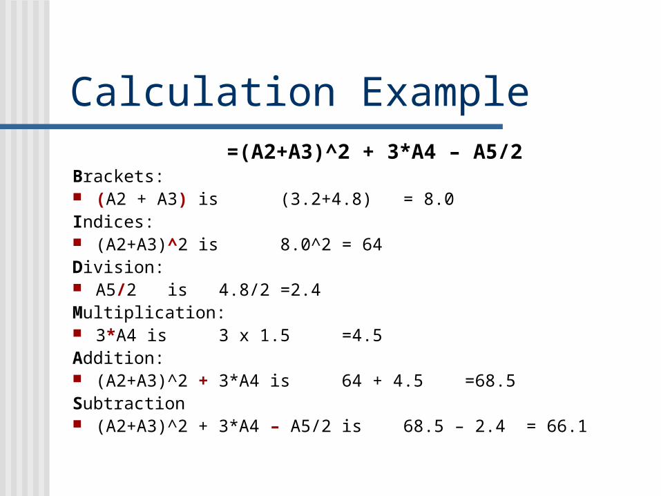
Calculation Example=(A2+A3)^2 + 3*A4 – A5/2
Brackets: (A2 + A3) is (3.2+4.8) = 8.0Indices: (A2+A3)^2 is 8.0^2 = 64Division: A5/2 is 4.8/2 =2.4Multiplication: 3*A4 is 3 x 1.5 =4.5Addition: (A2+A3)^2 + 3*A4 is 64 + 4.5 =68.5Subtraction (A2+A3)^2 + 3*A4 – A5/2 is 68.5 – 2.4 = 66.1
Calculations Example The spreadsheet
calculations.xls is a simple spreadsheet which will give you practice at constructing formulae
ActionPoint!
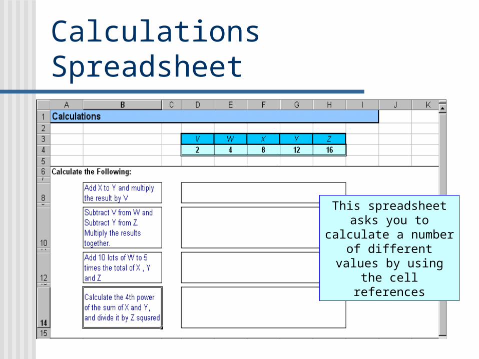
Calculations Spreadsheet
This spreadsheet asks you to calculate a number of different values by using the
cell references
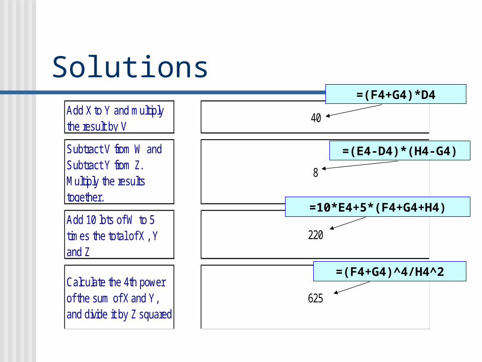
SolutionsAdd X to Y and multiply the result by V
Subtract V from W and Subtract Y from Z. Multiply the results together.
Add 10 lots of W to 5 times the total of X , Y and Z
Calculate the 4th power of the sum of X and Y, and divide it by Z squared
40
8
220
625
=(F4+G4)*D4
=(E4-D4)*(H4-G4)
=10*E4+5*(F4+G4+H4)
=(F4+G4)^4/H4^2

What happens when you copy and paste formulae? In the next few
slides we look at how the cell addresses change when they are copied into different locations
Cell Referencing A cell may be
referenced in one of four ways: An Absolute Address A Relative Address A Mixed Address Range Name
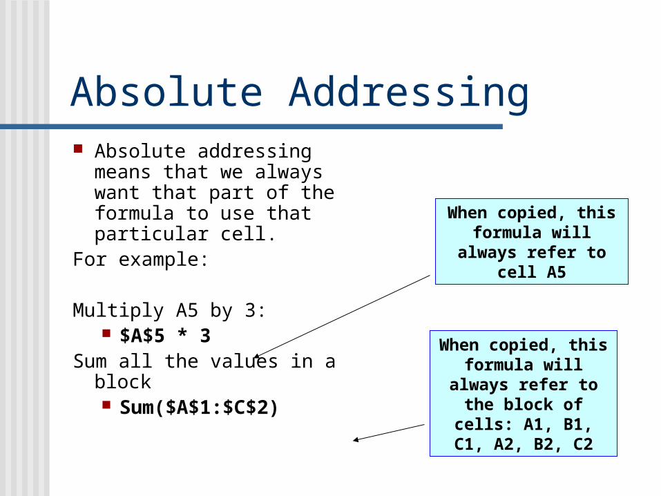
Absolute Addressing Absolute addressing
means that we always want that part of the formula to use that particular cell.
For example:
Multiply A5 by 3: $A$5 * 3
Sum all the values in a block Sum($A$1:$C$2)
When copied, this formula will
always refer to cell A5
When copied, this formula will
always refer to the block of cells:
A1, B1, C1, A2, B2, C2
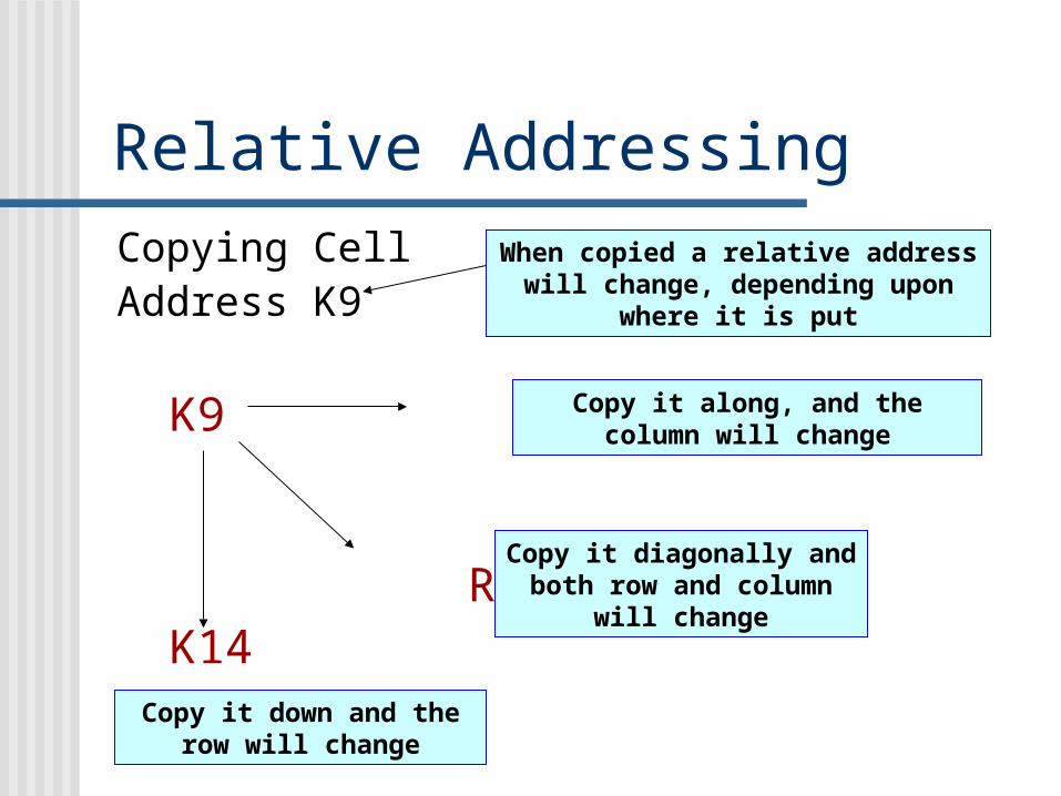
Relative AddressingCopying CellAddress K9
K9 Q9
R13K14
When copied a relative address will change, depending upon
where it is put
Copy it along, and the column will change
Copy it down and the row will change
Copy it diagonally and both row and column
will change
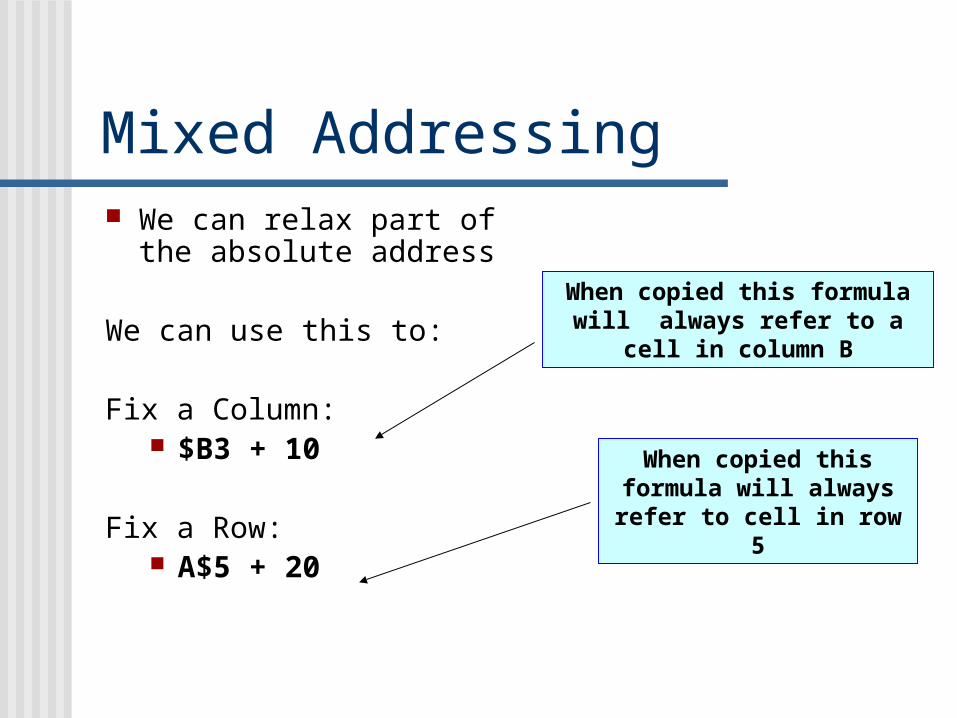
Mixed Addressing We can relax part of
the absolute address
We can use this to:
Fix a Column: $B3 + 10
Fix a Row: A$5 + 20
When copied this formula will always refer to a cell
in column B
When copied this formula will always refer to cell in row 5
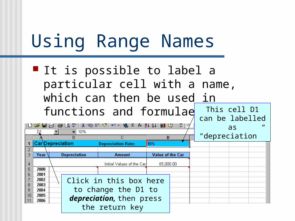
Using Range Names It is possible to label a particular cell
with a name, which can then be used in functions and formulae.
This cell D1 can be labelled as
“depreciation”
Click in this box here to change the D1 to
depreciation, then press the return key
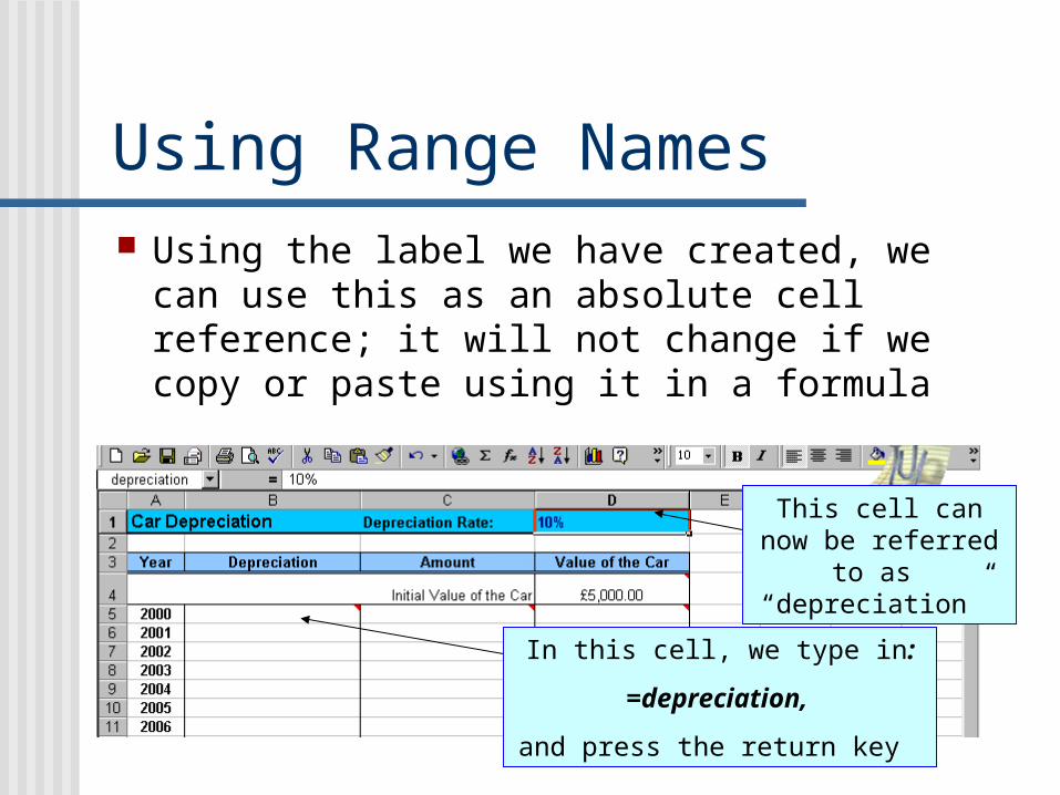
Using Range Names Using the label we have created, we
can use this as an absolute cell reference; it will not change if we copy or paste using it in a formula
This cell can now be referred to as “depreciation”
In this cell, we type in:
=depreciation,
and press the return key
Exploring Copy and Paste In the next few
examples we will carry out some simple financial calculations
Each time we will enter some formulae, then copy and paste these formulae to carry out the calculations in later cells
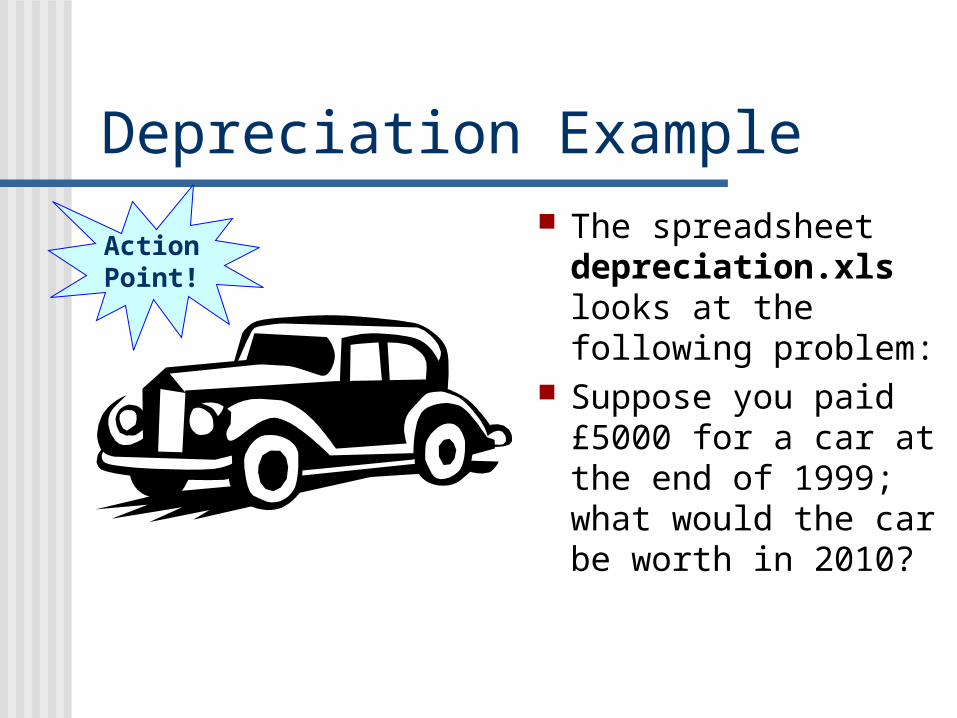
Depreciation Example The spreadsheet
depreciation.xls looks at the following problem:
Suppose you paid £5000 for a car at the end of 1999; what would the car be worth in 2010?
ActionPoint!
The Depreciation Spreadsheet
Car Depreciation Depreciation Rate: 10%
Year Depreciation Amount Value of the Car
£5,000.0020002001200220032004200520062007200820092010
Initial Value of the Car
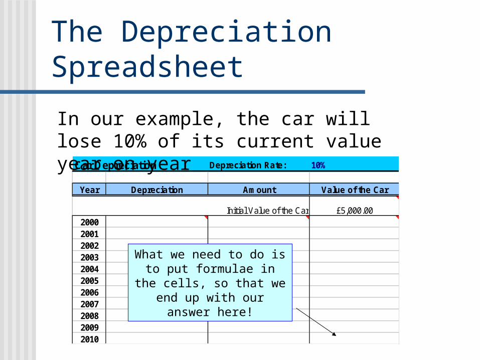
What we need to do is to put formulae in the cells, so that we end up with
our answer here!
In our example, the car will lose 10% of its current value year on year
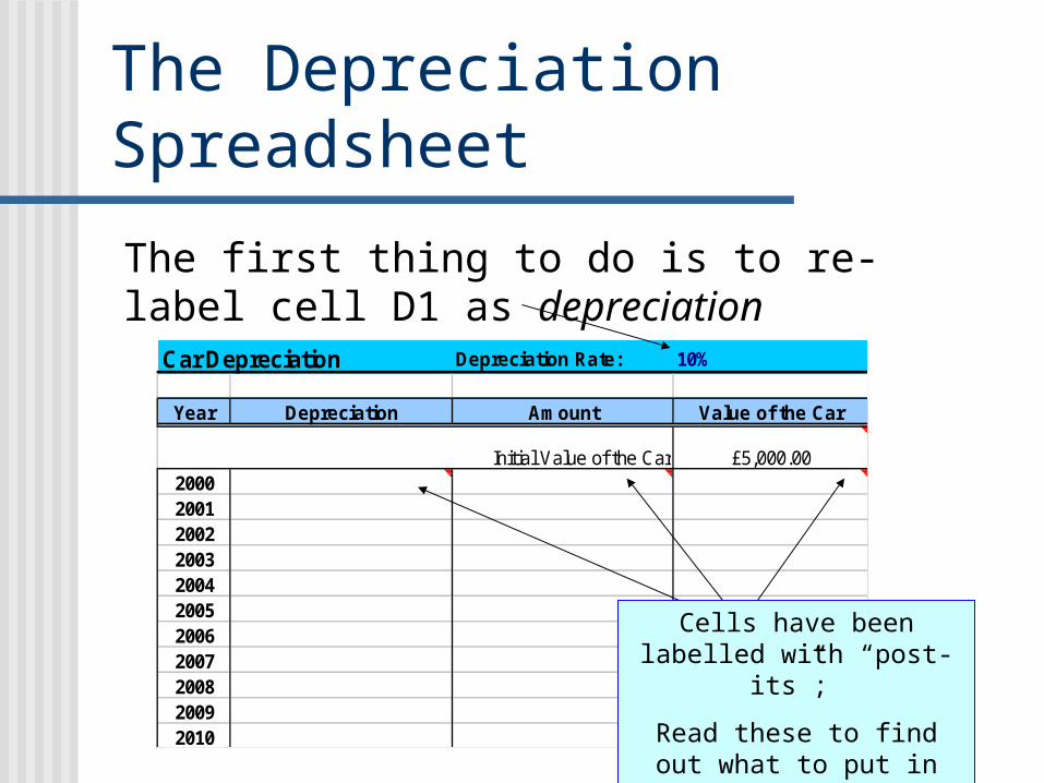
The Depreciation Spreadsheet
Car Depreciation Depreciation Rate: 10%
Year Depreciation Amount Value of the Car
£5,000.0020002001200220032004200520062007200820092010
Initial Value of the Car
Cells have been labelled with “post-its”;
Read these to find out what to put in the cells
The first thing to do is to re-label cell D1 as depreciation
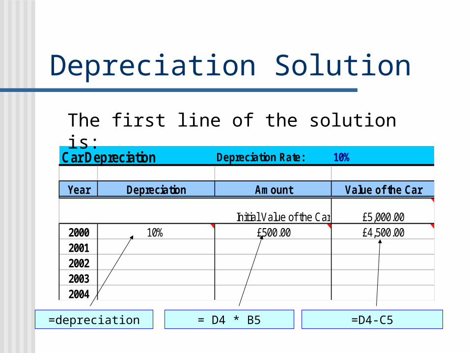
Car Depreciation Depreciation Rate: 10%
Year Depreciation Amount Value of the Car
£5,000.002000 10% £500.00 £4,500.002001200220032004
Initial Value of the Car
Depreciation Solution
=D4-C5=depreciation = D4 * B5
The first line of the solution is:
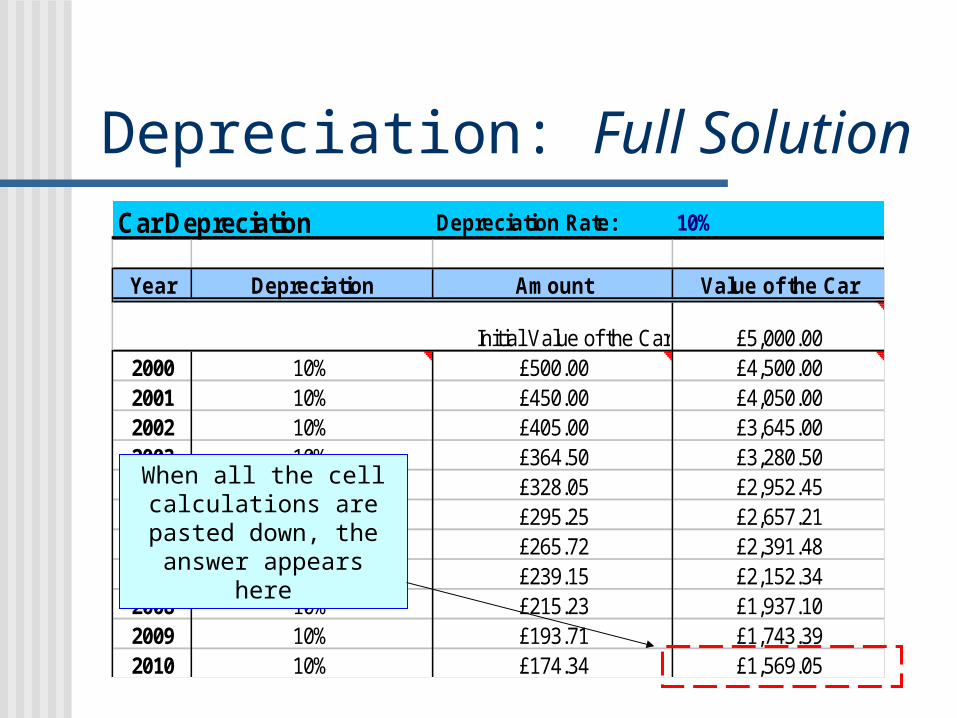
Depreciation: Full SolutionCar Depreciation Depreciation Rate: 10%
Year Depreciation Amount Value of the Car
£5,000.002000 10% £500.00 £4,500.002001 10% £450.00 £4,050.002002 10% £405.00 £3,645.002003 10% £364.50 £3,280.502004 10% £328.05 £2,952.452005 10% £295.25 £2,657.212006 10% £265.72 £2,391.482007 10% £239.15 £2,152.342008 10% £215.23 £1,937.102009 10% £193.71 £1,743.392010 10% £174.34 £1,569.05
Initial Value of the Car
When all the cell calculations are
pasted down, the answer appears here
Auditing Formulae Sometimes a
formula does not quite give you the answer that you wanted.
In this case you can use the auditing tools to check where the answer has originated
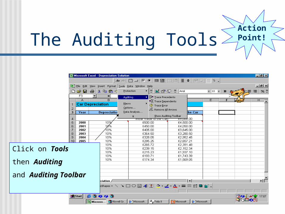
The Auditing Tools
Click on Tools
then Auditing
and Auditing Toolbar
ActionPoint!
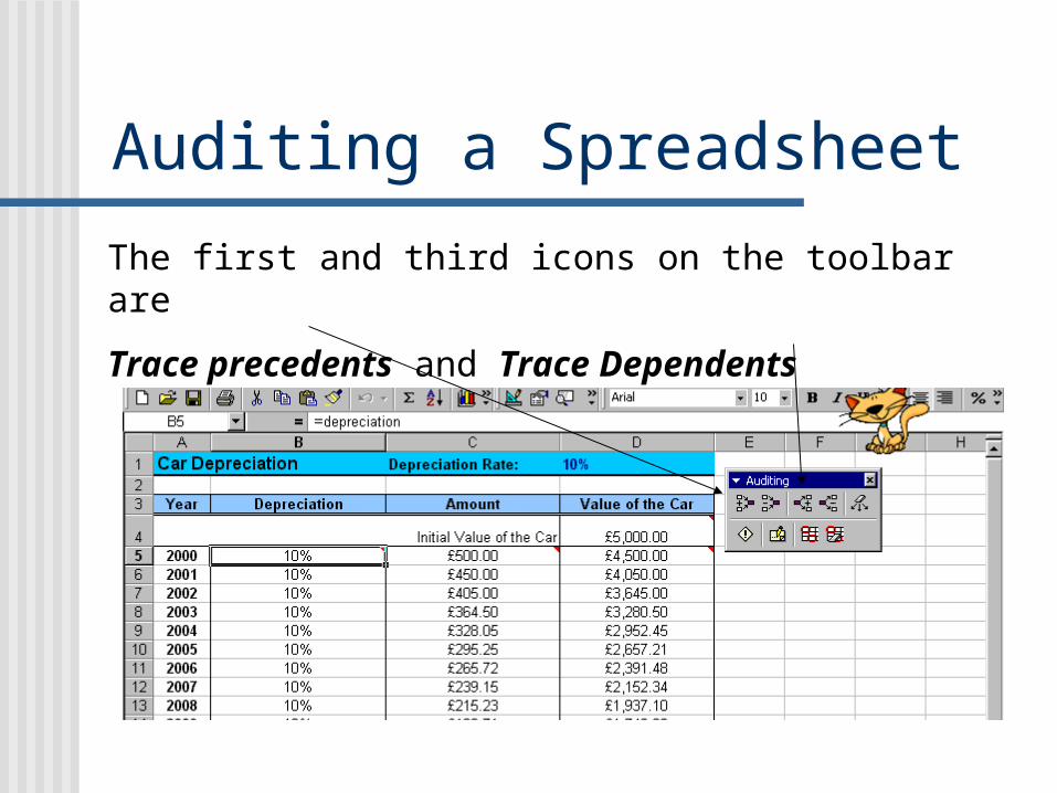
Auditing a Spreadsheet
The first and third icons on the toolbar are
Trace precedents and Trace Dependents
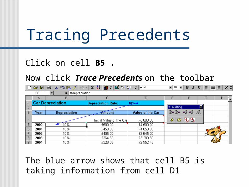
Tracing Precedents
Click on cell B5 .
Now click Trace Precedents on the toolbar
The blue arrow shows that cell B5 is taking information from cell D1
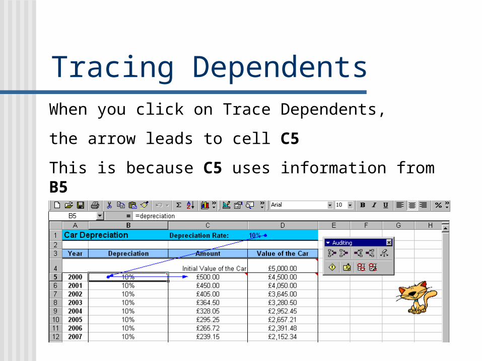
Tracing DependentsWhen you click on Trace Dependents,
the arrow leads to cell C5
This is because C5 uses information from B5
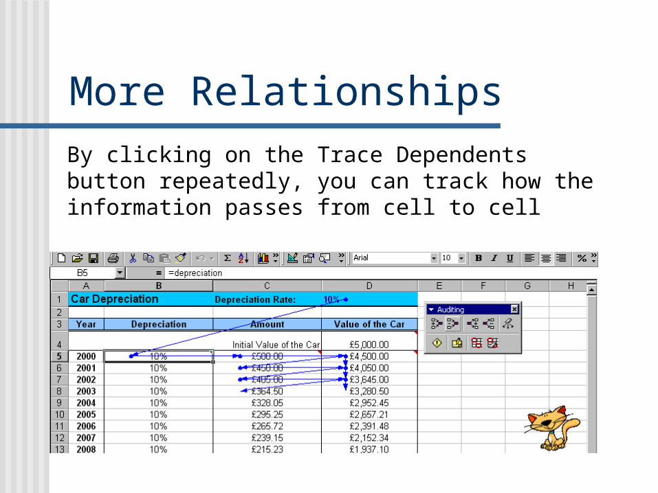
More RelationshipsBy clicking on the Trace Dependents button repeatedly, you can track how the information passes from cell to cell

Further Challenge To extend your
understanding of formulae, the next part of this presentation looks at copying and pasting across rows and down columns
It uses both relative and absolute addressing
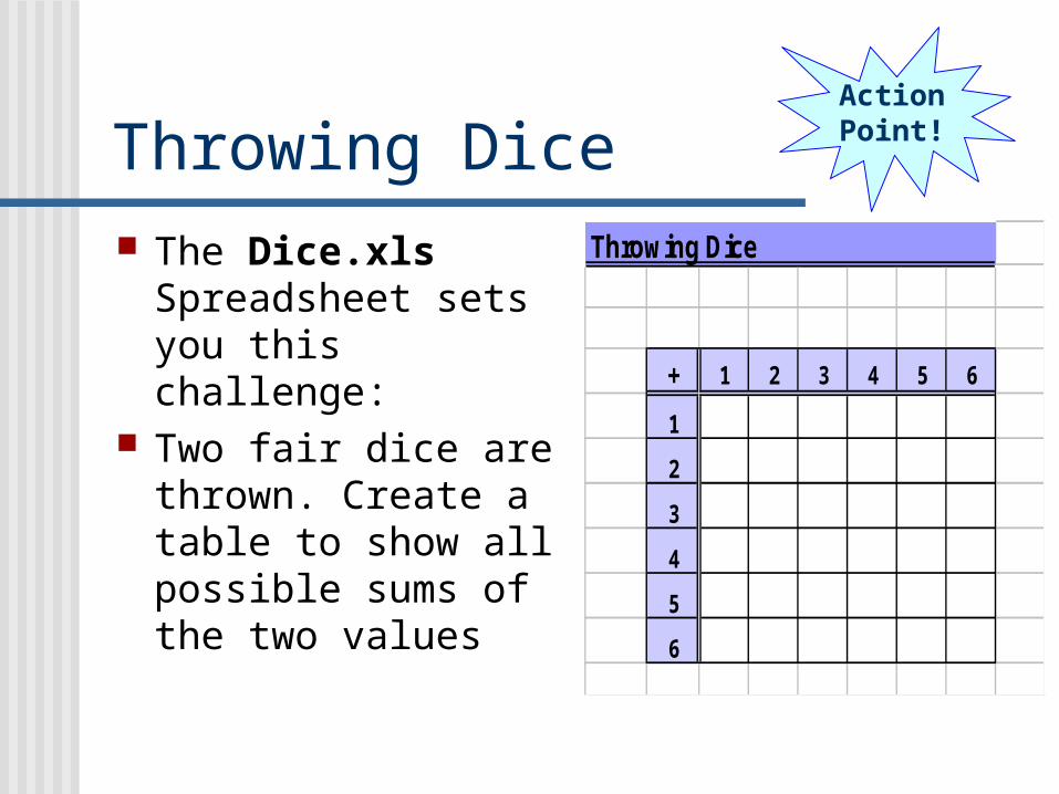
Throwing Dice The Dice.xls
Spreadsheet sets you this challenge:
Two fair dice are thrown. Create a table to show all possible sums of the two values
Throwing Dice
+ 1 2 3 4 5 6
1
2
3
4
5
6
ActionPoint!
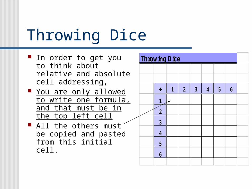
Throwing Dice In order to get you to
think about relative and absolute cell addressing,
You are only allowed to write one formula, and that must be in the top left cell
All the others must be copied and pasted from this initial cell.
Throwing Dice
+ 1 2 3 4 5 6
1
2
3
4
5
6
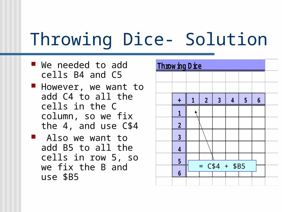
Throwing Dice- Solution We needed to add
cells B4 and C5 However, we want to
add C4 to all the cells in the C column, so we fix the 4, and use C$4
Also we want to add B5 to all the cells in row 5, so we fix the B and use $B5
Throwing Dice
+ 1 2 3 4 5 6
1
2
3
4
5
6= C$4 + $B5
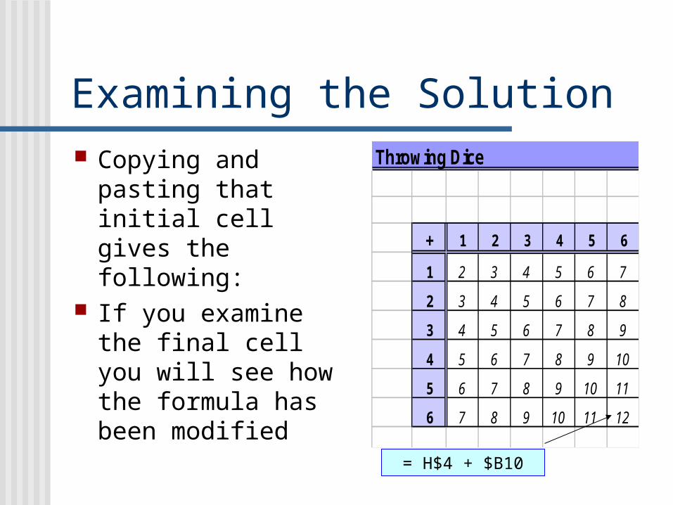
Examining the Solution Copying and
pasting that initial cell gives the following:
If you examine the final cell you will see how the formula has been modified
Throwing Dice
+ 1 2 3 4 5 6
1 2 3 4 5 6 7
2 3 4 5 6 7 8
3 4 5 6 7 8 9
4 5 6 7 8 9 10
5 6 7 8 9 10 11
6 7 8 9 10 11 12
= H$4 + $B10
Savings and Loans As a final example,
look at savings and loans.xls
This spreadsheet calculates interest on savings, loan repayments and mortgages.
You will need to work out the formulae
ActionPoint!

Follow-Up work Portfolio Task 2
now takes you through a scenario in which you create portfolios of shares to maximise your return on investment.