Spread options, Farkas’s lemma and linear programming

cutting edge derivatives pricing

35risk.net/life-and-pension-risk september 2011

OptiOns On individual underlyings are very liquid in a variety of markets. in many markets, moreover, options on linear combina-tions of underlyings are also reasonably liquid. Of primary interest to us are markets with liquid spread options (that is, options on the dif-ference of two underlyings), such as constant maturity swap (CMs) spread options in interest rate markets. Our discussion also naturally extends to other important examples such as foreign exchange markets with cross-rate options and equity markets with basket options, but we will concentrate on spread options from now on.

When spread options are available, it becomes important to be able to construct a joint distribution of two underlyings that is consistent with the spread option prices (and, naturally, with the marginal distribu-tions of the underlyings themselves). this problem has attracted increased attention recently, with possible constructions proposed in andersen & piterbarg (2010) and austing (2011). While it is very useful to be able to construct such distributions, these approaches suffer from at least two weaknesses. First, they are not guaranteed to produce a valid, in particular non-negative, probability density. and second, if these approaches fail, it does not necessarily mean that the joint distribution does not exist.

in this article, we derive necessary and sufficient conditions for the joint distribution with required properties to exist. the conditions turn out to have a deep financial meaning and can be formulated in terms of existence or absence of arbitrage among payouts of a certain type. From a practical perspective, we develop numerical methods to construct such joint distributions when they exist, and to find among all of them those that satisfy certain extremality criteria. Finally, we

develop numerical methods to construct payouts that realise arbitrage in the case where a joint distribution does not exist.

it should be noted that our results rely on the existence of a liquid market in options on spread options of all strikes, and also assume no bid-ask spread. these assumptions clearly do not hold in practice. nevertheless, such an idealised set-up is still valuable to develop a deeper understanding of the problem. Moreover, many trading desks mark spread options for a continuum of strikes for internal risk man-agement, and the tools we develop could be used to test these marks for internal inconsistencies.

Existencelet X and Y be two random variables representing two underlyings, and let S represent their spread. We assume their distributions are known from the options markets on X, Y and S.

let f(x), g(y) be two functions; we think of them as defining payouts on X and Y correspondingly. in particular, the value of an option on X with payout f(x) is E( f(X)) (here and everywhere discounting is ignored as we consider a fixed time horizon).

let us define the spread envelope of f, g by:

E f ,g z( ) = max

x−y=zf x( ) + g y( ){ }

the meaning of the spread envelope should be clear – it is the small-est function of x – y only that dominates the function f(x) + g(y) for all x, y:

Spread options, Farkas’s lemma and linear programming

How a joint distribution is constructed with given marginals is key to consistently pricing spread options. a classical result from probability ensures this can be done consistently

with the principle of no arbitrage – and an easily implementable numerical approach can provide the opportunity for spotting arbitrage opportunities.

By Vladimir Piterbarg

LPR0911_Technical.indd 35 02/09/2011 14:30

NOT FOR PUBLIC

ATION

Life & pension risk


36

E f ,g z( ) =min h z( ) : f x( ) + g y( ) ≤ h x − y( ){ }

if (X, Y) have a joint distribution such that X – Y has the same distri-bution as S, then we would clearly have:

E f X( )( )+ E g Y( )( ) ≤ E E f ,g X −Y( )( )

since by the no-arbitrage principle, if one payout is dominated by another, the value of the corresponding option is less. it turns out that the reverse is also true, and that is the main theoretical result of this article.■ Theorem. let three random variables X, Y, S be given. if for any continuous, bounded payouts f(⋅), g(⋅) we have that:

E f X( )( )+ E g Y( )( ) ≤ E E f ,g S( )( )

then, and only then, there exists a joint distribution of (X, Y) such that it has marginals X, Y and the distribution of X – Y is the same as S.

as promised above, the result has a clear financial interpretation. it states that if we cannot construct an arbitrage that involves an arbitrary payout f of X only, g of Y only and their spread envelope (a function of S only), then a joint distribution exists. it can also be seen as a conse-quence of the fundamental theorem of asset pricing (see duffie, 2001).

We provide a direct proof in a discrete setting in the appendix. the proof is based on the so-called Farkas’s lemma from convexity theory (see Farkas, 1902). the general statement of the theorem follows from the results in Gaffke & Rüschendorf (1984).

this result generalises ideas behind triangle arbitrage in spread options that is studied in McCloud (2011). triangle arbitrage is based on the observation that:

X −Kx( )+ − Y −Ky( )+ ≤ X −Y − Kx −Ky( )( )+

≤ X −Kx( )+ + Ky −Y( )+ (1)

for any strikes Kx, Ky, so if a joint distribution exists then the options on the spread must satisfy certain lower and upper bounds that depend on marginal distributions. Moreover, these bounds can be shown to be given by the Fréchet bounds on the copula that joins X and Y together (see McCloud, 2011, for details). the connection with our result is seen from the fact that the triangle inequality (1) is a special case of a spread envelope construction (for the lower bound we would take f(x) = (x – Kx)

+ and g(y) = –(y – Ky)+ and similar for the upper bound).

absence of triangle arbitrage is, however, not sufficient for the exist-ence of the joint distribution. in other words, we may have a situation

where triangle arbitrage is absent but more general spread envelope arbitrage still exists1 (see piterbarg, 2011, and below). it is an open question whether it is sufficient to check the no-arbitrage conditions in our theorem for only a subset of functions f, g.

Spread options by linear programmingOur theorem gives us a nice theoretical result with a strong financial interpretation, but from a practical perspective it is not very useful as it would be impossible to check for spread envelope arbitrage for all the payouts. Here, we develop a practical approach to the existence prob-lem and related questions. Given that in actual computer calculations we always work with discretised quantities, we assume that X, Y are

0 5 10 15 20 25 30 35 40

0.45

0.40

0.35

0.30

0.25

0.20

0.15

0.10

0.05

0

Low optionon index

High optionon index

2Densityofthesumoftworandomvariables,withthedistributionsofeachvariableandtheirdifferenceGaussian,optimisedtohavethehighestandthelowestvaluesoftheoptiononthesum

Joint density,low option on index

Joint density,high option on index

0.10

0.08

0.06

0.04

0.02

0

0.100.080.060.040.02

0

010

20

0

10

200 5 10 15 20 0 5 10 15 20

1JointdensityforGaussianmarginalsandGaussiandistributionofthespread,optimisedtohavethelowest(left)andthehighest(right)valueoftheoptionontheindex

1 Of course more complicated strategies will incur higher costs (through bid-ask spreads) in practice, as more options need to be traded. We briefly discuss bid-ask spreads below


NOT FOR PUBLIC

ATION

37


risk.net/life-and-pension-risk september 2011

discrete, with the support on the common grid {i/N, i = 0, ... , N}. We assume that S is on the grid ({i – N)/N, i = 0, ... , 2N}. let us denote the distributions of the three random variables by:

ri = P Y = N − i( ) / N( )cj = P X = j / N( )

dk = P S = k − N( ) / N( )

with i, j = 0, ... , N and k = 0, ... , 2N. vectors r, c, d are non-negative with the elements summing up to one. note that we label rows ri in

reverse order (that is, r0 corresponds to the maximum value of Y) for convenience and to reconcile the Cartesian view of the world (with the y-axis pointing upward) with the matrix indexing on computers where the row index increases in the downward direction.■ Existence. We can reformulate the existence question in the dis-crete setting as follows. let us see under what conditions on r, c, d there exists a matrix p = {pi,j}

Ni,j=0 such that:

pi, j ≥ 0, i, j = 0,...,N (2)

pi, j = ri , i = 0,...,N

j=0

N∑

(3)

0.12

0.10

0.08

0.06

0.04

0.02

00 5 10 15 20 25 30 35 40

High optionon index

Low optionon index

4Densityofthesumoftworandomvariables,withthedistributionsofeachvariableandtheirdifferenceGaussian,optimisedtobesmoothandtohavethehighestandthelowestvaluesoftheoptiononthesum

0

0.02

0.04

0.06

0.08

0.10

0.12

0.14

0.16

0.18

0 2 4 6 8 10 12 14 16 18–0.2

0

0.2

0.4

0.6

0.8

1.0Density of X (l-h side)Payout for X (r-h side)

%

Den

sity

of X

Payou

t for X

5DensityandpayoutfortheunderlyingXthatrealisesspreadenvelopearbitrage

0

0.05

0.10

0.15

0.20

0.25

0 2 4 6 8 10 12 14 16 18–0.2

0

0.2

0.4

0.6

0.8

1.0Density of Y (l-h side)Payout for Y (r-h side)

%

Den

sity

of Y

Payou

t for Y

6DensityandpayoutfortheunderlyingYthatrealisesspreadenvelopearbitrage

Joint density,low option on index

Joint density,high option on index

0.020

0.015

0.010

0.005

0

0.020

0.015

0.010

0.005

0010

20

0

10

200 5 10 15 20 0 5 10 15 20

3JointdensityforGaussianmarginalsandGaussiandistributionofthespread,optimisedtobesmoothandtohavethelowest(left)andthehighest(right)valueoftheoptionontheindex


NOT FOR PUBLIC

ATION

Life & pension risk38


pi, j = cj , j = 0,...,N

i=0

N∑

(4)

pi, j = dk , k = 0,...,2N

i, j( )∈Dk

∑

(5)

where Dk is the kth diagonal:

Dk = i, j( ) : i + j = k,0 ≤ i, j ≤ N{ }, k = 0,...,2N

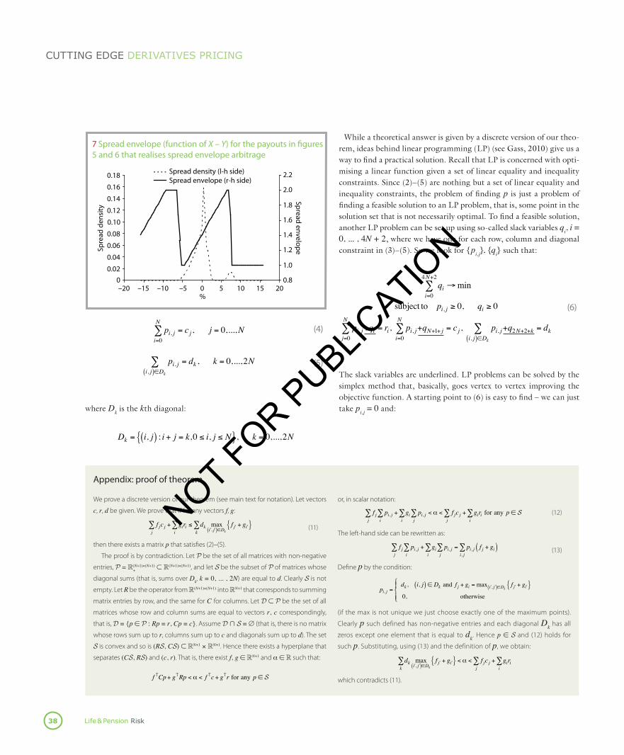
While a theoretical answer is given by a discrete version of our theo-rem, ideas behind linear programming (lp) (see Gass, 2010) give us a way to find a practical solution. Recall that lp is concerned with opti-mising a linear function given a set of linear equality and inequality constraints. since (2)–(5) are nothing but a set of linear equality and inequality constraints, the problem of finding p is just a problem of finding a feasible solution to an lp problem, that is, some point in the solution set that is not necessarily optimal. to find a feasible solution, another lp problem can be set up using so-called slack variables qi, i = 0, ... , 4N + 2, where we have one for each row, column and diagonal constraint in (3)–(5). so we look for {pi,j}, {qi} such that:

qi →mini=0

4N+2∑

subject to pi, j ≥ 0, qi ≥ 0

pi, j+qi = ri , pi, j+qN+1+ ji=0

N∑

j=0

N∑ = cj , pi, j+q2N+2+k = dk

i, j( )∈Dk

∑

(6)

the slack variables are underlined. lp problems can be solved by the simplex method that, basically, goes vertex to vertex improving the objective function. a starting point to (6) is easy to find – we can just take pi,j = 0 and:

We prove a discrete version of our theorem (see main text for notation). Let vectors

c, r, d be given. We prove that if for any vectors f, g:

f jc j + giri ≤ dk max

ʹ′i , ʹ′j( )∈Dkk∑

i∑

j∑ f ʹ′j + g ʹ′i{ }

(11)

then there exists a matrix p that satisfies (2)–(5).

The proof is by contradiction. Let P be the set of all matrices with non-negative

entries, P = R+(N+1)×(N+1) ⊂ R(N+1)×(N+1), and let S be the subset of P of matrices whose

diagonal sums (that is, sums over Dk, k = 0, ... , 2N) are equal to d. Clearly S is not

empty. Let R be the operator from R(N+1)×(N+1) into RN+1 that corresponds to summing

matrix entries by row, and the same for C for columns. Let D ⊂ P be the set of all

matrices whose row and column sums are equal to vectors r, c correspondingly,

that is, D = {p ∈ P : Rp = r, Cp = c}. Assume D ∩ S = ∅ (that is, there is no matrix

whose rows sum up to r, columns sum up to c and diagonals sum up to d). The set

S is convex and so is (RS, CS) ⊂ RN+1 × RN+1. Hence there exists a hyperplane that

separates (CS, RS) and (c, r). That is, there exist f, g ∈ RN+1 and a ∈ R such that:

fTCp+ gTRp < α < f Tc+ gTr for any p ∈ S

or, in scalar notation:

f j pi, j + gi pi, j < α < f jc j + giri for any p ∈ Si∑

j∑

j∑

i∑

i∑

j∑

(12)

The left-hand side can be rewritten as:

f j pi, j + gi pi, j = pi, j f j + gi( )

i, j∑

j∑

i∑

i∑

j∑

(13)

Define p by the condition:

pi, j =dk , i, j( ) ∈ Dk and f j + gi =max ʹ′i , ʹ′j( )∈Dk

f ʹ′j + g ʹ′i{ }0, otherwise

⎧⎨⎪

⎩⎪

(if the max is not unique we just choose exactly one of the maximum points).

Clearly p such defined has non-negative entries and each diagonal Dk has all

zeros except one element that is equal to dk. Hence p ∈ S and (12) holds for

such p. Substituting, using (13) and the definition of p, we obtain:

dk maxʹ′i , ʹ′j( )∈Dk

f ʹ′j + g ʹ′i{ } < α < f jc j + girii∑

j∑

k∑

which contradicts (11).

Appendix:proofoftheorem

0

0.02

0.04

0.06

0.08

0.10

0.12

0.14

0.16

0.18

–20 –15 –10 –5 0 5 10 15 200.8

1.0

1.2

1.4

1.6

1.8

2.0

2.2Spread density (l-h side)Spread envelope (r-h side)

%

Spre

ad d

ensi

ty

Spread

envelo

pe

7Spreadenvelope(functionofX–Y)forthepayoutsinfigures5and6thatrealisesspreadenvelopearbitrage


NOT FOR PUBLIC

ATION

39risk.net/life-and-pension-risk september 2011


qi =ri i ≤ N

ci−N−1 N +1≤ i ≤ 2N +1di−2N−2 2N + 2 ≤ i

⎧

⎨⎪⎪

⎩⎪⎪

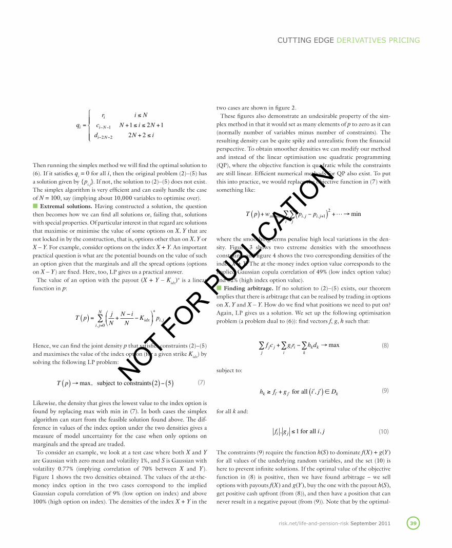
then running the simplex method we will find the optimal solution to (6). if it satisfies qi = 0 for all i, then the original problem (2)–(5) has a solution given by {pi,j}. if not, the solution to (2)–(5) does not exist. the simplex algorithm is very efficient and can easily handle the case of N = 100, say (implying about 10,000 variables to optimise over).■ Extremal solutions. Having constructed a solution, the question then becomes how we can find all solutions or, failing that, solutions with special properties. Of particular interest in that regard are solutions that maximise or minimise the value of some options on X, Y that are not locked in by the construction, that is, options other than on X, Y or X – Y. For example, consider options on the index X + Y. an important practical question is what are the potential bounds on the value of such an option given that the marginals and all the spread options (options on X – Y) are fixed. Here, too, lp gives us a practical answer.

the value of an option with the payout (X + Y – Kidx)+ is a linear

function in p:

T p( ) = jN+N − iN

−Kidx⎛

⎝⎜

⎞

⎠⎟+

i, j=0

N∑ pi, j

Hence, we can find the joint density p that satisfies constraints (2)–(5) and maximises the value of the index option (for a given strike Kidx) by solving the following lp problem:

T p( )→max, subject to constraints 2( )− 5( ) (7)

Likewise, the density that gives the lowest value to the index option is found by replacing max with min in (7). In both cases the simplex algorithm can start from the feasible solution found above. The dif-ference in values of the index option under the two densities gives a measure of model uncertainty for the case when only options on marginals and the spread are traded.

to consider an example, we look at a test case where both X and Y are Gaussian with zero mean and volatility 1%, and S is Gaussian with volatility 0.77% (implying correlation of 70% between X and Y). Figure 1 shows the two densities obtained. the values of the at-the-money index option in the two cases correspond to the implied Gaussian copula correlation of 9% (low option on index) and above 100% (high option on index). the densities of the index X + Y in the

two cases are shown in figure 2.these figures also demonstrate an undesirable property of the sim-

plex method in that it would set as many elements of p to zero as it can (normally number of variables minus number of constraints). the resulting density can be quite spiky and unrealistic from the financial perspective. to obtain smoother densities we can modify our method and instead of the linear optimisation use quadratic programming (Qp), where the objective function is quadratic while the constraints are still linear. Efficient numerical methods for Qp also exist. to put this into practice, we would replace the objective function in (7) with something like:

T p( )+wsmooth pi, j − pi, j+1( )2j∑

i∑ +L→min

where the smoothing terms penalise high local variations in the den-sity. Figure 3 shows two extreme densities with the smoothness constraints and figure 4 shows the two corresponding densities of the index X + Y. the at-the-money index option value corresponds to the implied Gaussian copula correlation of 49% (low index option value) and 82% (high index option value).■ Finding arbitrage. if no solution to (2)–(5) exists, our theorem implies that there is arbitrage that can be realised by trading in options on X, Y and X – Y. How do we find what positions we need to put on? again, lp gives us a solution. We set up the following optimisation problem (a problem dual to (6)): find vectors f, g, h such that:

f jc j + giri − hkdk

k∑

i∑

j∑ →max

(8)

subject to:

hk ≥ f ʹ′i + g ʹ′j for all ʹ′i , ʹ′j( ) ∈ Dk (9)

for all k and:

fi , gj ≤1 for all i, j (10)

the constraints (9) require the function h(S) to dominate f(X) + g(Y) for all values of the underlying random variables, and the set (10) is here to prevent infinite solutions. if the optimal value of the objective function in (8) is positive, then we have found arbitrage – we sell options with payouts f(X) and g(Y), buy the one with the payout h(S), get positive cash upfront (from (8)), and then have a position that can never result in a negative payout (from (9)). note that by the optimal-


NOT FOR PUBLIC

ATION

Life & pension risk40


ity property, the solution h will be the spread envelope of f and g.in practice, the existence of bid-ask spreads will clearly complicate

the construction of arbitrage strategies. While peña, vera & Zuluaga (2010) demonstrate how to add the consideration of bid-ask spreads to triangle arbitrage strategies (in the context of baskets on multiple underlyings), extending these ideas to arbitrary payouts that we con-sider in this article appears to be difficult.

an example solution is shown in figures 5, 6 and 7. this corresponds to CMs spread option prices observed in november 2010 in the euro. the spread density does not admit triangle arbitrage (or, equivalently, spread option prices satisfy lower/upper Fréchet bounds) but exhibit more general spread envelope arbitrage. the arbitrage profit from this strategy is of the order of a few basis points and in practice will not be realisable due to liquidity costs, yet the example is valuable as it high-lights potential arbitrage issues when marking spread option smiles.

ConclusionWe demonstrate that the existence of a joint distribution that is consist-ent with the marginal distributions of two underlyings and the distribution of the spread between them is intimately linked to the pres-ence or absence of arbitrage involving payouts on the underlyings and the spread – what we call the spread envelope arbitrage. We also propose practical numerical approaches based on lp to determine whether such a distribution exists. When it does exist, we show how to use lp meth-ods to find densities satisfying certain optimality conditions; that allows us to quantify a measure of model uncertainty in non-spread two-dimensional payouts. Moreover, we show how the lp methods could be used to find payouts that realise arbitrage when the joint distribution does not exist. While we focus on spread options, straightforward exten-sions can be made to basket options and options on cross forex rates.

there remain a number of questions. in particular, can we meaning-fully restrict the set of payouts for which we should check no-arbitrage conditions to guarantee the existence of a joint distribution? Or, more generally, is there a set of sufficient conditions for existence that is easier to check? Finally, is there a theoretical description, perhaps cop-ula-like, of all distributions that match given marginals and the spread distribution? L&pr

VladimirPiterbargisglobalheadofquantitativeanalyticsatBarclaysCapital.

Email:[email protected]

Andersen L and V Piterbarg, 2010Interest rate modeling, in three volumesAtlantic Financial Press

Austing P, 2011Repricing the cross smile: an analytic joint densityRisk July, pages 72–75

Duffie D, 2001Dynamic asset pricing theoryPrinceton University Press

Farkas J, 1902Über die theorie der einfachen ungleichungenJournal für die Reine und Angewandte Mathematik 124, pages 1–27

Gaffke N and L Rüschendorf, 1984On the existence of probability measures with given marginals

Statistics and Decisions 2, pages 163–174

Gass S, 2010Linear programming: methods and applicationsDover Publications, fifth edition

McCloud P, 2011The CMS triangle arbitrageRisk January, pages 126–131

Peña J, J Vera and L Zuluaga, 2010Computing arbitrage upper bounds on basket options in the presence of bid-ask spreadsSubmitted to European Journal of Operational Research

Piterbarg V, 2011Spread options and Farkas’ lemmaICBI Conference, Paris

References

Life & Pension Risk welcomes the submission of technical articles on topics relevant to

our readership. Core areas include market and credit risk measurement and manage-

ment, the pricing and hedging of derivatives and/or structured securities, and the

theoretical modelling and empirical observation of markets and portfolios. This list

is not exhaustive.

The most important publication criteria are originality, exclusivity and relevance

– we attempt to strike a balance between these. Given that Life & Pension Risk techni-

cal articles are shorter than those in dedicated academic journals, clarity of exposi-

tion is another yardstick for publication. Once received by the technical editor and

his team, submissions are logged and checked against these criteria. Articles that fail

to meet the criteria are rejected at this stage.

Articles are then sent without author details to one or more anonymous refe-

rees for peer review. Our referees are drawn from the research groups, risk manage-

ment departments and trading desks of major financial institutions, in addition to

academia. Many have already published articles in Life & Pension Risk. Authors

should allow four to eight weeks for the refereeing process. Depending on the

feedback from referees, the author may attempt to revise the manuscript. Based on

this process, the technical editor makes a decision to reject or accept the submit-

ted article. His decision is final.

Submissions should be sent, preferably by email, to the technical team (technical@

incisivemedia.com).

Microsoft Word is the preferred format, although PDFs are acceptable if submitted

with LaTeX code or a word file of the plain text. It is helpful for graphs and figures to

be submitted as separate Excel, postscript or EPS files.

The maximum recommended length for articles is 3,500 words, with some allow-

ance for charts and/or formulas. We expect all articles to contain references to previ-

ous literature. We reserve the right to cut accepted articles to satisfy production

considerations.

Guidelinesforthesubmissionoftechnicalarticles


NOT FOR PUBLIC

ATION

Documents

Spread options, Farkas’s lemma and linear programming