Embed Size (px)
Citation preview

Evaluation of the Cost Benefits of Continuous Pavement Preservation Design Strategies Versus Reconstruction
Final Report 491 Prepared by: K.L. Smith, L. Titus-Glover, M.I. Darter, H.L. Von Quintus, R.N. Stubstad, and J.P. Hallin Applied Research Associates 505 W. University Ave. Champaign, Illinois 68120
September 2005 Prepared for: Arizona Department of Transportation in cooperation with U.S. Department of Transportation Federal Highway Administration

DISCLAIMER The contents of this report reflect the views of the authors who are responsible for the facts and the accuracy of the data presented herein. The contents do not necessarily reflect the official views or policies of the Arizona Department of Transportation or the Federal Highway Administration. This report does not constitute a standard, specification, or regulation. Trade or manufacturers' names which may appear herein are cited only because they are considered essential to the objectives of the report. The U.S. Government and the State of Arizona do not endorse products or manufacturers.
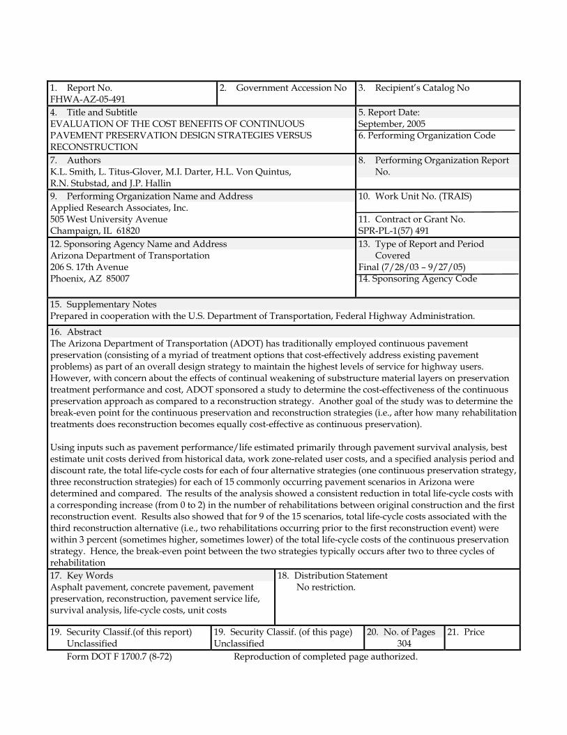
1. Report No. FHWA-AZ-05-491
2. Government Accession No
3. Recipient’s Catalog No
4. Title and Subtitle EVALUATION OF THE COST BENEFITS OF CONTINUOUS PAVEMENT PRESERVATION DESIGN STRATEGIES VERSUS RECONSTRUCTION
5. Report Date: September, 2005 6. Performing Organization Code
7. Authors K.L. Smith, L. Titus-Glover, M.I. Darter, H.L. Von Quintus, R.N. Stubstad, and J.P. Hallin
8. Performing Organization Report No.
9. Performing Organization Name and Address Applied Research Associates, Inc. 505 West University Avenue Champaign, IL 61820
10. Work Unit No. (TRAIS) 11. Contract or Grant No. SPR-PL-1(57) 491
12. Sponsoring Agency Name and Address Arizona Department of Transportation 206 S. 17th Avenue Phoenix, AZ 85007
13. Type of Report and Period Covered
Final (7/28/03 – 9/27/05) 14. Sponsoring Agency Code
15. Supplementary Notes Prepared in cooperation with the U.S. Department of Transportation, Federal Highway Administration.
16. Abstract The Arizona Department of Transportation (ADOT) has traditionally employed continuous pavement preservation (consisting of a myriad of treatment options that cost-effectively address existing pavement problems) as part of an overall design strategy to maintain the highest levels of service for highway users. However, with concern about the effects of continual weakening of substructure material layers on preservation treatment performance and cost, ADOT sponsored a study to determine the cost-effectiveness of the continuous preservation approach as compared to a reconstruction strategy. Another goal of the study was to determine the break-even point for the continuous preservation and reconstruction strategies (i.e., after how many rehabilitation treatments does reconstruction becomes equally cost-effective as continuous preservation). Using inputs such as pavement performance/life estimated primarily through pavement survival analysis, best estimate unit costs derived from historical data, work zone-related user costs, and a specified analysis period and discount rate, the total life-cycle costs for each of four alternative strategies (one continuous preservation strategy, three reconstruction strategies) for each of 15 commonly occurring pavement scenarios in Arizona were determined and compared. The results of the analysis showed a consistent reduction in total life-cycle costs with a corresponding increase (from 0 to 2) in the number of rehabilitations between original construction and the first reconstruction event. Results also showed that for 9 of the 15 scenarios, total life-cycle costs associated with the third reconstruction alternative (i.e., two rehabilitations occurring prior to the first reconstruction event) were within 3 percent (sometimes higher, sometimes lower) of the total life-cycle costs of the continuous preservation strategy. Hence, the break-even point between the two strategies typically occurs after two to three cycles of rehabilitation 17. Key Words Asphalt pavement, concrete pavement, pavement preservation, reconstruction, pavement service life, survival analysis, life-cycle costs, unit costs
18. Distribution Statement No restriction.
19. Security Classif.(of this report) Unclassified
19. Security Classif. (of this page) Unclassified
20. No. of Pages 304
21. Price
Form DOT F 1700.7 (8-72) Reproduction of completed page authorized.

SI* (MODERN METRIC) CONVERSION FACTORS
APPROXIMATE CONVERSIONS TO SI UNITS APPROXIMATE CONVERSIONS FROM SI UNITS Symbol When You Know Multiply By To Find Symbol Symbol When You Know Multiply By To Find Symbol
LENGTH LENGTH
in inches 25.4 millimeters mm mm millimeters 0.039 inches in
ft feet 0.305 meters m m meters 3.28 feet ft yd yards 0.914 meters m m meters 1.09 yards yd mi miles 1.61 kilometers km km kilometers 0.621 miles mi AREA AREA
in2 square inches 645.2 square millimeters mm2 mm2 Square millimeters 0.0016 square inches in2
ft2 square feet 0.093 square meters m2 m2 Square meters 10.764 square feet ft2
yd2 square yards 0.836 square meters m2 m2 Square meters 1.195 square yards yd2 ac acres 0.405 hectares ha ha hectares 2.47 acres ac mi2 square miles 2.59 square kilometers km2 km2 Square kilometers 0.386 square miles mi2
VOLUME VOLUME fl oz fluid ounces 29.57 milliliters mL mL milliliters 0.034 fluid ounces fl oz gal gallons 3.785 liters L L liters 0.264 gallons gal ft3 cubic feet 0.028 cubic meters m3 m3 Cubic meters 35.315 cubic feet ft3
yd3 cubic yards 0.765 cubic meters m3 m3 Cubic meters 1.308 cubic yards yd3
NOTE: Volumes greater than 1000L shall be shown in m3. MASS MASS
oz ounces 28.35 grams g g grams 0.035 ounces oz lb pounds 0.454 kilograms kg kg kilograms 2.205 pounds lb T short tons (2000lb) 0.907 megagrams
(or “metric ton”) mg
(or “t”) Mg megagrams
(or “metric ton”) 1.102 short tons (2000lb) T
TEMPERATURE (exact) TEMPERATURE (exact) ºF Fahrenheit
temperature 5(F-32)/9
or (F-32)/1.8 Celsius temperature ºC ºC Celsius temperature 1.8C + 32 Fahrenheit
temperature ºF
ILLUMINATION ILLUMINATION fc foot candles 10.76 lux lx lx lux 0.0929 foot-candles fc fl foot-Lamberts 3.426 candela/m2 cd/m2 cd/m2 candela/m2 0.2919 foot-Lamberts fl FORCE AND PRESSURE OR STRESS FORCE AND PRESSURE OR STRESS
lbf poundforce 4.45 newtons N N newtons 0.225 poundforce lbf lbf/in2 poundforce per
square inch 6.89 kilopascals kPa kPa kilopascals 0.145 poundforce per
square inch lbf/in2
SI is the symbol for the International System of Units. Appropriate rounding should be made to comply with Section 4 of ASTM E380

TABLE OF CONTENTS EXECUTIVE SUMMARY .....................................................................................i CHAPTER 1 INTRODUCTION.........................................................................1 BACKGROUND AND PROBLEM DESCRIPTION...........................................................1 PROJECT OBJECTIVES AND SCOPE .................................................................................2 OVERVIEW OF REPORT.......................................................................................................2 CHAPTER 2 DATA COLLECTION AND DATABASE DEVELOPMENT....................................................................................................5 INTRODUCTION ...................................................................................................................5 DATA COLLECTION ............................................................................................................5 DATABASE DEVELOPMENT..............................................................................................7 DATA SUMMARY................................................................................................................19 SUMMARY OF DATA USED IN PERFORMANCE ANALYSIS ..................................43 CHAPTER 3 PAVEMENT PERFORMANCE ANALYSIS..........................49 INTRODUCTION .................................................................................................................49 PAVEMENT SURVIVAL ANALYSIS................................................................................49 MECHANISTIC-BASED PERFORMANCE ANALYSIS.................................................76 CHAPTER 4 ANALYSIS OF CONSTRUCTION COSTS...........................93 INTRODUCTION .................................................................................................................93 DEVELOPMENT OF BEST ESTIMATES OF COSTS.......................................................93 CHAPTER 5 USER COST BEST PRACTICES............................................107 INTRODUCTION ...............................................................................................................107 USER DELAY COSTS ASSOCIATED WITH WORK ZONES......................................107 VEHICLE OPERATING COSTS ASSOCIATED WITH SMOOTHNESS ...................109

TABLE OF CONTENTS (CONTINUED) CHAPTER 6 DEVELOPMENT OF LIFE-CYCLE MODELS.....................113 INTRODUCTION ...............................................................................................................113 ANALYSIS CELL 1 .............................................................................................................118 ANALYSIS CELL 2 .............................................................................................................120 ANALYSIS CELL 3 .............................................................................................................122 ANALYSIS CELL 4 .............................................................................................................124 ANALYSIS CELL 5 .............................................................................................................126 ANALYSIS CELL 6 .............................................................................................................128 ANALYSIS CELL 7 .............................................................................................................131 ANALYSIS CELL 8 .............................................................................................................133 ANALYSIS CELL 9 .............................................................................................................136 ANALYSIS CELL 10 ...........................................................................................................138 ANALYSIS CELL 11 ...........................................................................................................140 ANALYSIS CELL 12 ...........................................................................................................142 ANALYSIS CELL 13 ...........................................................................................................144 ANALYSIS CELL 14 ...........................................................................................................146 ANALYSIS CELL 15 ...........................................................................................................148 CHAPTER 7 LIFE-CYCLE COST ANALYSIS.............................................151 INTRODUCTION ...............................................................................................................151 LCCA APPROACH AND SOFTWARE...........................................................................151 LCCA INPUTS.....................................................................................................................152 SUMMARY OF LCCA RESULTS .....................................................................................164 CHAPTER 8 CONCLUSIONS AND RECOMMENDATIONS ..............181 CONCLUSIONS..................................................................................................................182 RECOMMENDATIONS.....................................................................................................185 REFERENCES .....................................................................................................187 APPENDIX A PAVEMENT SURVIVAL CURVES................................... A-1

v
LIST OF FIGURES Figure Page 1. Establishment of activities/structures for 1-mi PMS pavement sections.................8 2. Construction date histogram for CAC pavement sections .......................................25 3. Age histogram for CAC pavement sections................................................................26 4. Traffic histogram for CAC pavement sections ...........................................................26 5. Asphalt thickness histogram for CAC pavement sections .......................................27 6. Construction date histogram for DSAC pavement sections.....................................29 7. Age histogram for DSAC pavement sections .............................................................29 8. Traffic histogram for DSAC pavement sections.........................................................30 9. Asphalt thickness histogram for DSAC pavement sections .....................................31 10. Construction date histogram for FDAC pavement sections.....................................32 11. Age histogram for FDAC pavement sections .............................................................33 12. Traffic histogram for FDAC pavement sections.........................................................34 13. Asphalt thickness histogram for FDAC pavement sections .....................................34 14. Construction date histogram for JPC pavement sections .........................................36 15. Age histogram for JPC pavement sections..................................................................36 16. Traffic histogram for JPC pavement sections .............................................................37 17. Slab thickness histogram for JPC pavement sections ................................................37 18. Construction date histogram for JPCD pavement sections ......................................39 19. Age histogram for JPCD pavement sections...............................................................39 20. Traffic histogram for JPCD pavement sections ..........................................................40 21. Slab thickness histogram for JPCD pavement sections .............................................40 22. Construction date histogram for CRC pavement sections........................................42 23. Age histogram for CRC pavement sections ................................................................42 24. Traffic histogram for CRC pavement sections............................................................43 25. Age histogram for CAC, DSAC, and FDAC pavement sections .............................45 26. Traffic histogram for CAC, DSAC, and FDAC pavement sections .........................45 27. Asphalt thickness histogram for CAC, DSAC, and FDAC pavement sections .....46 28. Age histogram for JPC, JPCD, and CRC pavement sections ....................................47 29. Traffic histogram for JPC, JPCD, and CRC pavement sections................................47 30. Slab thickness histogram for JPC, JPCD, and CRC pavement sections ..................48 31. Plot of the standard normal distribution.....................................................................54 32. Comparison of median service life estimates (LIFEREG) for original asphalt pavements, based on age and cumulative truck applications..................................61 33. Comparison of median service life estimates (LIFEREG) for original concrete pavements, based on age and cumulative truck applications..................................61 34. Comparison of median age-based initial service life estimates obtained using non-parametric (LIFETEST) and parametric (LIFEREG) procedures .....................63 35. Comparison of median truck-based initial service life estimates obtained using non-parametric (LIFETEST) and parametric (LIFEREG) procedures...........63

LIST OF FIGURES (CONTINUED) Figure Page 36. Performance of conventional asphalt mix when used in different structure- defined rehabilitations applied to Interstate asphalt pavements.............................71 37. Performance of conventional asphalt mix when used in different structure- defined rehabilitations applied to Non-Interstate asphalt pavements....................72 38. Performance of thin conventional overlays (R1) on asphalt pavement using different asphalt mixture types .....................................................................................72 39. Performance of shallow removal and thin overlays (R3) on asphalt pavement using different asphalt mixture types ..........................................................................73 40. Performance of shallow removal and thick overlays (R4) on asphalt pavement using different asphalt mixture types ..........................................................................73 41. Performance of deep removal and thick overlays (R6) on asphalt pavement using different asphalt mixture types ..........................................................................74 42. Performance of conventional asphalt and asphalt rubber mixes when used in thin conventional overlay of JPC pavements .........................................................75 43. Comparison of median age-based rehabilitation life estimates obtained using non-parametric (LIFETEST) and parametric (LIFEREG) procedures ..........75 44. Comparison of median truck-based rehabilitation life estimates obtained using non-parametric (LIFETEST) and parametric (LIFEREG) procedures ..........76 45. Predicted versus measured cracking (longitudinal and fatigue) for CAC at SHRP site 04-1006 (I-10, Maricopa County, MP 110.65)............................................83 46. Predicted versus measured transverse joint faulting for JPC at SHRP site 04-7613 (SR 360, Maricopa County, MP 7.42) .............................................................83 47. Histogram showing 50 percent survival life estimated from ADOT performance data and M-E evaluation of typical ADOT flexible pavements........92 48. Histogram showing 50 percent survival life estimated from ADOT performance data and M-E evaluation of typical ADOT rigid pavements............92 49. Unit cost histogram for pay item 3030022, class 2 aggregate base (AB) (based on 1999 Construction Costs report) .................................................................98 50. Unit cost histogram for pay item 4140040, asphalt rubber used in asphalt rubber friction course (FR) (based on 1999 Construction Costs report) .................98 51. Unit cost histogram for asphalt rubber (AR) binder pay item (based on Asphalt Rubber Projects report)..................................................................................101 52. Unit cost histogram for asphalt rubber (AR) mixture pay item (based on Asphalt Rubber Projects report)..................................................................................101 53. Unit cost histogram for asphalt rubber friction course (FR) binder pay item (based on Asphalt Rubber Projects report) ...............................................................102 54. Unit cost histogram for asphalt rubber friction course (FR) mixture pay item (based on Asphalt Rubber Projects report) ...............................................................102 55. Impact of pavement roughness on vehicle speed ....................................................110

LIST OF FIGURES (CONTINUED) Figure Page 56. Conceptual illustration of continuous preservation and reconstruction design strategies ............................................................................................................117 57. Life-cycle models for analysis cell 1—CAC interstate pavement, hot-dry climate.............................................................................................................................119 58. Life-cycle models for analysis cell 2—CAC interstate pavement, moderate climate.............................................................................................................................121 59. Life-cycle models for analysis cell 3—CAC non-interstate pavement, hot-dry climate.............................................................................................................................123 60. Life-cycle models for analysis cell 4—CAC non-interstate pavement, moderate climate ...........................................................................................................125 61. Life-cycle models for analysis cell 5—CAC non-interstate pavement, cool-wet climate.............................................................................................................................127 62. Life-cycle models for analysis cell 6—DSAC interstate pavement, hot-dry climate.............................................................................................................................129 63. Life-cycle models for analysis cell 7—DSAC interstate pavement, moderate climate.............................................................................................................................132 64. Life-cycle models for analysis cell 8—DSAC interstate pavement, cool-wet climate.............................................................................................................................134 65. Life-cycle models for analysis cell 9—DSAC non-interstate pavement, hot-dry climate.............................................................................................................................137 66. Life-cycle models for analysis cell 10—DSAC non-interstate pavement, moderate climate ...........................................................................................................139 67. Life-cycle models for analysis cell 11—DSAC non-interstate pavement, cool-wet climate.............................................................................................................141 68. Life-cycle models for analysis cell 12—JPC pavement, hot-dry climate...............143 69. Life-cycle models for analysis cell 13—JPC pavement, cool-wet climate.............145 70. Life-cycle models for analysis cell 14—JPCD pavement, hot-dry climate............147 71. Life-cycle models for analysis cell 15—CRC pavement, hot-dry climate.............149 72. NPV distribution generation (Smith and Walls, 1998) ............................................152 73. Default hourly distribution used in analysis (for rural and urban project site locations) ........................................................................................................................158 74. Agency and user costs for each iteration for analysis cell 1 ...................................169 75. Agency and user costs for each iteration for analysis cell 2 ...................................169 76. Agency and user costs for each iteration for analysis cell 3 ...................................170 77. Agency and user costs for each iteration for analysis cell 4 ...................................170 78. Agency and user costs for each iteration for analysis cell 5 ...................................171 79. Agency and user costs for each iteration for analysis cell 6 ...................................171 80. Agency and user costs for each iteration for analysis cell 7 ...................................172
LIST OF FIGURES (CONTINUED) Figure Page 81. Agency and user costs for each iteration for analysis cell 8 ...................................172 82. Agency and user costs for each iteration for analysis cell 9 ...................................173 83. Agency and user costs for each iteration for analysis cell 10 .................................173 84. Agency and user costs for each iteration for analysis cell 11 .................................174 85. Agency and user costs for each iteration for analysis cell 12 .................................174 86. Agency and user costs for each iteration for analysis cell 13 .................................175 87. Agency and user costs for each iteration for analysis cell 14 .................................175 88. Agency and user costs for each iteration for analysis cell 15 .................................176 89. Effect of discount rate on cost difference between continuous preservation and reconstruction alternatives...................................................................................176 90. Effect of analysis period on cost difference between continuous preservation and reconstruction alternatives...................................................................................177 91. Percent change in NPV between continuous preservation and reconstruction for all analysis cells (alternatives 1 through 3) .........................................................180

LIST OF TABLES Table Page 1. Description of pavement preservation activity/material codes ..............................12 2. Categorization of M&R treatments for asphalt pavements ......................................13 3. Categorization of M&R treatments for concrete pavements ....................................17 4. Summary of the number of pavement sections along with facility types ..............20 5. Overview of pavement sections used in analysis ......................................................21 6. Highway breakdown of pavement sections analyzed for initial service life .........22 7. Types of rehabilitation activities performed according to pavement and facility types.....................................................................................................................23 8. Location breakdown of CAC pavement sections.......................................................24 9. Location breakdown of DSAC pavement sections.....................................................28 10 Location breakdown of FDAC pavement sections ....................................................32 11 Location breakdown of JPC pavement sections .........................................................35 12 Location breakdown of JPCD pavement sections ......................................................38 13 Location breakdown of CRC pavement sections .......................................................41 14 Summary of pavement sections included in databases for analysis .......................44 15 Initial pavement survival analysis matrix...................................................................56 16 Age-based survival analysis results for original/reconstructed pavements .........57 17 Revised pavement survival analysis matrix ...............................................................58 18 Age-based survival analysis results for newly constructed and reconstructed pavements ........................................................................................................................60 19 Truck traffic-based survival analysis results for newly constructed and reconstructed pavements ...............................................................................................60 20 Age-based survival results for structure-defined rehabilitation categories...........65 21 Truck traffic-based survival results for structure-defined rehabilitation categories .........................................................................................................................66 22 Age-based survival results for structure/mixture-defined rehabilitation categories..........................................................................................................................67 23 Truck traffic-based survival results for structure/mixture-defined rehabilitation categories .................................................................................................69 24 Description of the LTPP pavement sections used in developing the virtual pavements for analysis...................................................................................................78 25 Key pavement properties required for mechanistic-based evaluation for typical CAC and DSAC/FDAC pavements located in Arizona ..............................79 26 Key pavement properties required for mechanistic-based evaluation for typical JPC pavements located in Arizona..................................................................80 27 Key pavement properties required for mechanistic-based evaluation for typical JPCD pavements located in Arizona...............................................................81
LIST OF TABLES (CONTINUED) Table Page 28 Key pavement properties required for mechanistic-based evaluation for typical CRC pavements located in Arizona ................................................................82 29 Typical range of surface layer thickness, traffic, and subgrade properties used in developing “typical” pavements ....................................................................85 30 Performance indicators along with terminal values based on facility type used in analysis ...............................................................................................................85 31 Predictions of time and traffic loadings to failure for original or reconstructed CAC pavements, determined using NCHRP Project 1-37A performance models...............................................................................................................................86 32 Predictions of time and traffic loadings to failure for original or reconstructed DSAC/FDAC pavements, determined using NCHRP Project 1-37A performance models .......................................................................................................87 33 Predictions of time and traffic loadings to failure for original or reconstructed JPC pavements, determined using NCHRP Project 1-37A performance models...............................................................................................................................88 34 Predictions of time and traffic loadings to failure for original or reconstructed JPCD pavements, determined using NCHRP Project 1-37A performance models...............................................................................................................................89 35 Predictions of time and traffic loadings to failure for original or reconstructed CRC pavements, determined using NCHRP Project 1-37A performance models...............................................................................................................................90 36 Survival analysis results of service life data obtained from M-E evaluation of “typical” pavements .......................................................................................................91 37 Sample data obtained from Construction Costs report (ADOT, 1999) ...................94 38 Sample data obtained from Asphalt Rubber Projects report (ADOT, 2002) ..........95 39 Inflation-adjusted unit costs for pay items in 1999 Construction Costs report .....96 40 Inflation-adjusted and quantity-filtered unit costs for pay items in 1999 Construction Costs report..............................................................................................99 41 Inflation-adjusted and quantity-filtered unit costs for pay items in Asphalt Rubber Projects report..................................................................................................104 42 Inflation-adjusted, in-place unit costs of various pay items contained in ADOT Pavement Management Cost Estimate .........................................................104 43 Comparison of inflation-adjusted and quantity–filtered unit costs derived from various cost data sources....................................................................................105 44 Effect of pavement serviceability/roughness on vehicle operating costs ............111 45 Typical initial pavement structures corresponding to 15 revised analysis cells ................................................................................................................................114 46 Typical M&R treatments corresponding to 15 revised analysis cells....................115 47 Summary of the selections made for the Analysis Options module .....................154
LIST OF TABLES (CONTINUED) Table Page 48 Summary of traffic information used in LCCA........................................................157 49 Summary of pay item unit costs used to estimate event/activity costs ...............160 50 Summary of user work zone unit costs .....................................................................162 51 Example calculation of agency maintenance costs ..................................................162 52 Summary of NPV at mean and 90 percent probability ...........................................165

LIST OF TERMS AND ACRONYMS TERMS Analysis Period—Time period over which the initial and future costs are evaluated for different design alternatives. Discount Rate—The rate used in economic analysis to represent the real value of money over time. It is a function of both the interest rate and inflation rate, and is used to convert future costs to present-day costs and/or present-day costs to annualized costs. (Highway) Agency Costs—Costs incurred directly by an owner agency over the life of a highway project. Agency costs are generally subdivided into three groups: initial cost, future costs, and salvage value. (Highway) User Costs—Costs incurred by the highway user over the life of a highway project. The user costs of concern are the differential or extra costs incurred by the traveling public as a result of one highway design being used instead of another. User cost categories typically include time delay costs, vehicle operating costs, accident costs, and discomfort costs associated with work zones or normal operating conditions. Life-Cycle Cost Analysis—An economic technique that allows comparisons of investment alternatives having different cost streams. In the highway arena, it is a formal, systematic approach for considering most of the factors that go into making a pavement investment decision. Life-Cycle Model—Depiction of the sequence of activities expected for a given pavement design alternative, from the initial structure to the final M&R treatment. In a life-cycle model, the type and timing of each anticipated activity is indicated, along with the expected quantities. (Pavement) Preservation—The planned strategy of cost-effective pavement treatments to an existing roadway to extend the life or improve the serviceability of a pavement. It is a program strategy intended to arrest deterioration, retard progressive failure, and improve the functional or structural capacity of the pavement. It is a strategy for individual pavements and for optimizing the performance of a pavement network. (Pavement) Service Life—The period of time over which no major cost events (i.e., rehabilitation, reconstruction) are required in providing a reasonable level of service to users.

(Pavement) Survival Analysis—A statistical analysis technique used to determine the expected service life of pavements and/or the performance of rehabilitation techniques. The procedure involves computing and graphing the probability of a pavement remaining without need of a rehabilitation or reconstruction event, based on historical pavement event data. ACRONYMS AC Asphalt Concrete ADT Average Daily Traffic CAC Conventional Asphalt Concrete CRC Continuously Reinforced Concrete DSAC Deep-Strength Asphalt Concrete FDAC Full-Depth Asphalt Concrete HMA OL Hot-Mix Asphalt Overlay JPC Jointed Plain Concrete, Nondoweled JPCD Jointed Plain Concrete, Doweled LCCA Life-Cycle Cost Analysis M&R Maintenance and Rehabilitation PCC Portland Cement Concrete PMS Pavement Management System RF Regional Factor VOC Vehicle Operating Cost
i
EXECUTIVE SUMMARY The Arizona Department of Transportation (ADOT) has a long and valuable history of highway pavement preservation. The Department has utilized and benefited greatly from the findings of past research concerning the cost-effectiveness of timely and appropriate forms of pavement preservation. Its current overall design strategy entails a continuous preservation approach, whereby one of a myriad of treatment options is selected based on its ability to cost-effectively address existing pavement conditions and future forecasted traffic loadings. With concern about the effects of continual weakening of substructure material layers on preservation treatment performance and cost, this study was conducted to assess the appropriateness of the continuous preservation approach as compared to a total reconstruction approach. The evaluation was made in terms of total life-cycle costs, as determined by pavement service life and construction costs, M&R treatment performance and costs, user delay associated with work zones, and the discount rate. The study also sought to determine the break-even point for the two design strategies (i.e., the point at which reconstruction becomes equally cost-effective as continuous preservation), so as to better allocate the funding of construction and preservation activities. To compute and compare the life-cycle costs of the two approaches, a detailed assessment of the key inputs of the life-cycle cost analysis (LCCA) process was made. First, using historical pavement project information and statewide pavement management data, the performance characteristics of six different pavement types—conventional asphalt concrete (CAC), deep-strength AC (DSAC), full-depth AC (FDAC), non-doweled jointed plain concrete (JPC), doweled JPC (JPCD), and continuously reinforced concrete (CRC) pavement—and numerous maintenance and rehabilitation (M&R) treatment types were analyzed. This analysis was done using pavement survival analysis techniques, supplemented by mechanistic-based performance modeling. The resulting information was then used to construct life-cycle models for 15 different scenarios representative of Arizona highway pavements and conditions. Second, a detailed analysis of construction and M&R unit costs was performed using data from three separate cost sources. Best estimates of the unit costs were then made based on the availability and reliability of data and engineering judgment. Lastly, a review of user cost components and models was made, with recommendations developed regarding the best practices for Arizona conditions.

ii
All of the resulting information was entered into the FHWA LCCA spreadsheet program RealCost, whereby the probabilistic life-cycle costs of continuous preservation and reconstruction alternatives were computed for each of the 15 pavement scenarios using a 4 percent discount rate and 60-year analysis period. Results indicated a consistent reduction in total life-cycle costs corresponding to an increase (from 0 to 2) in the number of rehabilitations between initial construction and the first reconstruction. Moreover, for a majority of scenarios evaluated, it was found that the total life-cycle costs associated with the third reconstruction alternative (two rehabilitations prior to reconstruction) were within 5 percent (sometimes higher, sometimes lower) of the total life-cycle costs of the continuous preservation strategy. Thus, it was determined that the break-even point between the continuous preservation strategy and the reconstruction strategy typically occurs after two to three cycles of rehabilitation (i.e., reconstruction preceded by two to three sequential rehabilitation treatments).
1
CHAPTER 1. INTRODUCTION BACKGROUND AND PROBLEM DESCRIPTION The term “pavement preservation” has been in use in the transportation facilities field for many years. Although its meaning has varied over time and among pavement practitioners, it is still often viewed in the sense described by the American Association of State Highway and Transportation Officials (AASHTO):
The planned strategy of cost-effective pavement treatments to an existing roadway to extend the life or improve the serviceability of a pavement. It is a program strategy intended to arrest deterioration, retard progressive failure, and improve the functional or structural capacity of the pavement. It is a strategy for individual pavements and for optimizing the performance of a pavement network.
Thus, pavement preservation represents an umbrella of activities, ranging from preventive maintenance treatments, such as slurry seals and chip seals, to minor rehabilitation treatments, like diamond grinding of Portland cement concrete (PCC) pavements and thin asphalt concrete (AC) overlays, to major rehabilitation treatments, such as extensive full-depth PCC repairs with or without diamond grinding and thick AC overlays with or without cold-milling. The Arizona Department of Transportation (ADOT) has a long and valuable history of highway pavement preservation. Beginning in the early to mid-1970s, the Department began shifting its focus from extensive patching and crack filling (corrective measures designed to hold a pavement together until reconstruction) to resurfacing (a type of preservation) in the form of an AC overlay or milling followed by AC overlay. Preservation funding increased in the years thereafter, and the implementation of a pavement management system in the early 1980’s helped researchers confirm the benefits of a preservation approach and evaluate the effectiveness of different preservation treatments (Way, 1983). Today, the Department has a large arsenal of preservation treatments that are used on a continuous basis to keep highways facilities fully operational and in good serviceable condition. The treatments selected for use are based on an extensive evaluation of the functional and structural conditions of the existing pavement and the long-term traffic forecasted for the facility. The treatments are generally designed for a 10-year performance life and a heavy emphasis is placed on the re-use of materials. The appropriateness of the continuous pavement preservation approach is a matter that the Department has recently deemed worthy of investigation. With rehabilitation activities taking place every 10 to 15 years, the direct costs of these activities add up
2
quickly and could be undercut by the costs of a construct–reconstruct approach having longer periods between interventions. Such a reconstruct approach would also appear to provide benefit in the arena of user costs, in that fewer interventions could translate into less time delay for highway users. This project investigates the legitimacy and cost practicality of the continuous preservation design philosophy, as compared to the construct–reconstruct approach. It involves a thorough evaluation of the performance and costs of ADOT pavement structures and rehabilitation treatments, followed by comprehensive life-cycle cost analyses (LCCAs) to determine the conditions or circumstances favorable to one approach over the other. PROJECT OBJECTIVES AND SCOPE The overall objective of this research project is to evaluate the cost benefit of continued pavement preservation design strategies, as compared to pavement reconstruction. The evaluation is to result in the identification of the best pavement design strategies available, based on total life cycle cost, and in the development of criteria for determining the break-even point between pavement preservation and reconstruction. The original scope of the research project consisted of seven primary tasks, as listed below.
• Task 1—Review Pavement Design Strategies and Performance Characteristics. • Task 2—Analyze ADOT’s Construction Costs for Typical Design Strategies. • Task 3—Evaluate Best Practices for User Costs. • Task 4—Develop Life-Cycle Models and Conduct LCCA. • Task 5—Develop Design Strategy and Selection Model Recommendations. • Task 6—Prepare Final Report. • Task 7—Prepare Research Note.
An eighth task, involving the performance evaluation of cold in-place recycling (CIR) projects, was subsequently added to the study. A separate report on this investigation was prepared and submitted to ADOT. OVERVIEW OF REPORT This report is presented in eight chapters. Chapter 1 is this introduction. Chapter 2 discusses the data collection and database development work. Descriptions of the pavement performance analyses conducted and the corresponding results are provided in chapter 3. Chapters 4 and 5 present the findings of the analysis of construction costs

3
and user cost practices, respectively. Chapters 6 and 7 feature the life-cycle models and LCCA results for the alternative pavement design strategies (continuous pavement preservation versus reconstruction). Finally, an overall summary of the conclusions and recommendations regarding design strategies is discussed in chapter 8. This report also includes one appendix. Appendix A contains survival curves for the various pavement structures and rehabilitation treatments examined in the study.

4
5
CHAPTER 2. DATA COLLECTION AND DATABASE DEVELOPMENT
INTRODUCTION In order to satisfy the project objectives, an intensive data collection and processing effort was undertaken. This effort involved obtaining the latest highway pavement databases and hardcopy records from ADOT, manually and electronically uploading the data into Microsoft® Access 2002, reviewing the accuracy and completeness of the data, and, where possible, adding new or replacement data. This chapter describes in detail the database development process leading to the establishment of datasets for pavement performance analysis. It describes the work performed in collecting the required data, building the project database, and reviewing and cleaning it for use in the study. It also presents a summary of the project data in terms of the types of pavements (new/reconstructed and rehabilitated) analyzed and their breakdowns by facility type, highway, ADOT District, construction year and age, traffic, and surface layer thickness. DATA COLLECTION Two electronic databases and various other data records from ADOT were used to build the project database. These information sources included the project history database, the pavement management system (PMS) database, the 2002 State highway log, the 1997 traffic composition table, a SuperPave asphalt mix design project list, and a project list for doweled, jointed plain concrete (JPCD) pavement. A brief description of each of these sources is provided in the sections below. Project History Database ADOT’s project history database was provided as a Microsoft Access® database management file. The database included information on over 5,800 construction/ rehabilitation projects undertaken on Arizona highways between 1928 and 2003. Key data fields included the following:
• ADOT construction project number. • ADOT District. • Highway number, direction, and lane. • Project limits (begin and end mileposts). • Activity/structure information, in terms of layer material types and thicknesses.
6
PMS Database ADOT’s PMS database was also provided as a Microsoft Access® database management file. Over 7,200, 1-mi long pavement sections covering all five interstate routes, 17 U.S. routes, and 82 State routes, were included in this database. Key data fields included the following:
• Highway number, type (e.g., alternate, business, spur), direction, and lane. • Section beginning milepost (established on 1-mi intervals [e.g., 1.0, 2.0, 3.0]). • ADOT District. • Regional factor (RF). • Average daily traffic (ADT) for years 1974 through 2002. • Traffic growth factors for years 2000, 2001, and 2002. • Year of most recent condition survey. • Pavement cracking quantities for years 1979 through 2002. • Smoothness measurements for years 1972 through 2002. • Pavement rutting measurements for years 1986 through 2002. • Pavement patching quantities for years 1979 through 2002. • Pavement flushing quantities for years 1979 through 2002. • Average maintenance costs for years 1979 through 2002.
2002 Highway Log This electronic file provided useful general information about the 100+ Arizona highways. It included overall mileage (centerline miles and lane miles) information for each highway facility, as well as linear referencing (mile markers, mileposts), geometric (number of lanes, lane widths, shoulder widths) and surfacing (travel lane and shoulder surface types) data for specifically-defined segments of each route. Also available were ADT and truck percentages for individual traffic count segments for the years 1997 through 2001. 1997 Traffic Composition Table Although the PMS database included extensive historical traffic data, the need existed for information on the number or percentage of trucks that pass over Arizona highways. Hence, ADOT provided in hardcopy form a detailed traffic table containing vehicle composition and equivalent single-axle load (ESAL) information for traffic count segments on all highways included in the PMS database. Data from this table were manually entered into Microsoft Excel® for ultimate incorporation into the project database. The data fields entered included highway number and traffic section milepost limits, the percentage of trucks in the overall vehicle population, and the percentage of medium and heavy trucks (FHWA vehicle

7
classes 4 through 13) in the overall truck population. Two-way annual traffic growth rates, derived from 1991 and 1997 ADT data, were also included. Using the above information, the percentage of medium and heavy trucks in the overall vehicle population was computed. The resulting percentages were subsequently used in conjunction with the annual ADT values in the PMS database to yield annual numbers of trucks. SuperPave Mix Design Project List With the Department’s expressed interest in the evaluation of its SuperPave asphalt mixes, the project database needed to specify the pavement sections containing a SuperPave mix. For this purpose, a listing of about 30 different SuperPave projects performed throughout Arizona between 1997 and 2001 was provided by ADOT. Although this list included detailed information about each mix design, the information of primary use was the ADOT construction project number, the project bid date, and the project location information (i.e., highway and milepost limits, benchmark/reference points). With these data and the activity/structure information given in the project history database, identification was made as to the rehabilitation projects that included a SuperPave mix. JPCD Project List Because the project history database did not list any JPCD projects, even though several such sections had been built between 1984 and 2001, a detailed list of JPCD projects was developed and provided by ADOT. This list contained general information, including ADOT construction project number, highway number and milepost limits, and completion dates, on about 25 projects constructed between 1984 and 2003. The information was used with the activity/structure information given in the project history database to indicate whether or not a 1-mi PMS section was built as JPCD. DATABASE DEVELOPMENT Development of the project database entailed seven key steps. These steps included the following:
1. Merging the ADOT project history and PMS databases. 2. Assigning event and pavement type codes to the pavement structures. 3. Adding important information on SuperPave and JPCD projects performed in
recent years. 4. Incorporating key traffic data (ADT growth rates and percent trucks) into the
database. 5. Performing detailed quality control (QC) checks of the data.
8
6. Assigning broad-based maintenance and rehabilitation (M&R) treatment codes to the thousands of recorded M&R activities.
7. Performing quality assurance (QA) checks of the data using statistical procedures.
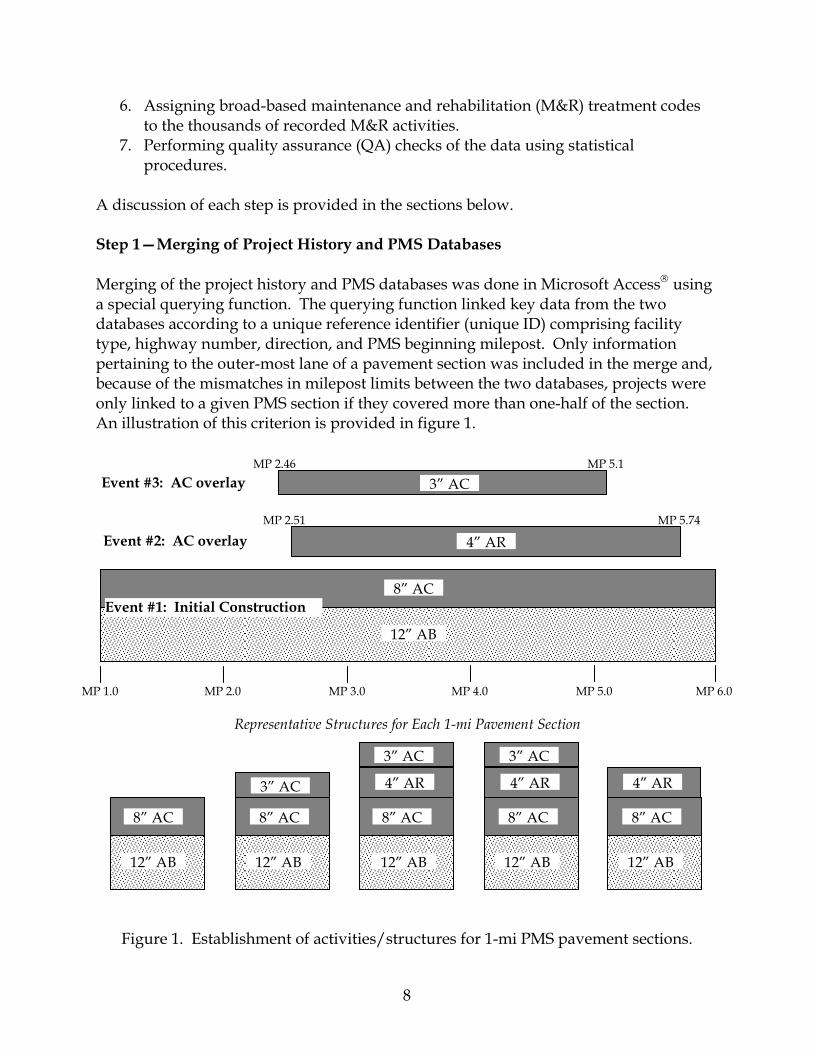
A discussion of each step is provided in the sections below. Step 1—Merging of Project History and PMS Databases Merging of the project history and PMS databases was done in Microsoft Access® using a special querying function. The querying function linked key data from the two databases according to a unique reference identifier (unique ID) comprising facility type, highway number, direction, and PMS beginning milepost. Only information pertaining to the outer-most lane of a pavement section was included in the merge and, because of the mismatches in milepost limits between the two databases, projects were only linked to a given PMS section if they covered more than one-half of the section. An illustration of this criterion is provided in figure 1.
Figure 1. Establishment of activities/structures for 1-mi PMS pavement sections.
MP 1.0 MP 2.0 MP 3.0 MP 4.0 MP 5.0 MP 6.0
MP 2.51 MP 5.74
MP 2.46 MP 5.1
12” AB
8” AC
Event #3: AC overlay
Event #2: AC overlay
12” AB
8” AC
3” AC
4” AR
12” AB 12” AB 12” AB 12” AB
8” AC 8” AC 8” AC 8” AC
4” AR 4” AR 4” AR 3” AC
3” AC 3” AC
Representative Structures for Each 1-mi Pavement Section
Event #1: Initial Construction

9
Step 2—Assigning Event and Pavement Type Codes The first part of this step entailed assigning an event code to each individual event (i.e., construction, rehabilitation, maintenance) that took place over time on each 1-mi pavement section. These event codes aided the performance analysis process. New or reconstructed pavement structures were assigned the code “O” (“original” structure), rehabilitation treatments were assigned the code “R,” and maintenance treatments were assigned the code “M.” The “O” codes were subsequently expanded to “O1,” “O2,” “O3,” etc., to reflect the sequence number of each original structure that a pavement section received. In the second part of this step, pavement type codes were assigned to each event, designating the basic type of pavement structure constructed or in existence at the time of an M&R treatment. A total of eight different pavement types were identified in the database, based on the following definitions:
• Conventional asphalt concrete (CAC)—Hot-mix asphalt (HMA) surface constructed over an untreated aggregate base/subbase course and prepared subgrade. The criterion used to define CAC pavements were that the total asphalt layer thickness had to be less than 7.5 in and could constitute no more than 40 percent of the total structure thickness (i.e., combined thickness of asphalt surface and aggregate base/subbase).
• Conventional asphalt concrete with treated base/subbase (CACT)—HMA surface constructed over a cement- or lime-treated aggregate base/subbase course and prepared subgrade.
• Deep-strength asphalt concrete (DSAC)—HMA surface constructed on HMA base and/or asphalt-treated base, an untreated aggregate base/subbase, and prepared subgrade. The criterion used to define DSAC pavements were that the total asphalt layer thickness had to be at least 4.5 in and could not constitute less than 40 percent of the total structure thickness (i.e., combined thickness of asphalt surface and aggregate base/subbase).
• Deep-strength asphalt concrete with treated base/subbase (DSACT)—HMA surface constructed on cement- or lime-treated aggregate base/subbase, and prepared subgrade.
• Full-depth asphalt concrete (FDAC)—HMA surface constructed on HMA base and/or asphalt-treated base (with variable percentage asphalt content) and prepared subgrade.
• Non-doweled jointed plain concrete (JPC)—Portland cement concrete (PCC) surface constructed over a treated or untreated base and prepared subgrade. The PCC can also be constructed directly over the subgrade. The PCC layer typically contains joints to control cracks expected in the concrete. For non-doweled JPC, dowel bars are not used to enhance load transfer at transverse joints. However, steel tie bars are generally used at longitudinal joints (lane-to-lane and lane-to-

10
PCC shoulder) to prevent excessive joint openings and to enhance longitudinal joint load transfer.
• Doweled jointed plain concrete (JPCD)—Similar to JPC with the exception that dowel bars are used to enhance load transfer at transverse contraction joints.
• Continuously reinforced concrete (CRC)—PCC surface with continuous longitudinal steel reinforcement and no intermediate transverse expansion or contraction joints constructed over a treated or untreated base and subgrade. The PCC can also be constructed directly over the subgrade.
Step 3—Designation of SuperPave and JPCD Projects This step simply entailed changing the activity/material codes for pavement sections where SuperPave mixes were used in the asphalt overlay or where dowels were used in the new/reconstructed concrete pavement. For sections with SuperPave, the code “AC” was replaced with “AC*.” For sections in which dowels were used, the code “PC” was changed to “PD.” Step 4—Addition of Traffic Composition and Growth Rate Data In this step, the percentage of medium and heavy trucks in the overall vehicle population was added to the project database, along with the 2-way annual traffic growth rate. Because this information existed according to traffic count segments that varied in length and did not match the PMS section limits, a querying function was developed and used to extrapolate the traffic data across the 1-mi PMS sections. Step 5—Performing QC Checks of Data Following the completion of step 4, the database was thoroughly and meticulously reviewed to identify missing and anomalous/erroneous data. Specific items looked for and addressed were missing pavement sections, inconsistencies within a pavement section between the original pavement type and the sequence of M&R activities, missing or clearly inaccurate layer type and thickness information, and questionable time intervals (too short or too long) between events. Most of the data issues identified were attributed to (a) missing or erroneous data in the project history and PMS databases and (b) extrapolation errors that occurred during the merging of the two databases. With regard to the former, efforts were made to either obtain the appropriate data from ADOT or to use sound engineering judgment to develop reasonable estimates of the missing/erroneous data. Where neither approach was deemed adequate, the subject pavement section was removed from the database. With regard to the latter, merging information from the two databases according to a common lane was sometimes problematic where multi-lane, urban highways were

11
involved. This was because any time a lane was added as part of an event, the lane designation for the lane of interest (the outermost lane) changed. To rectify this situation, a detailed review was made of the event sequence and time-series performance data for all sections comprised by multiple lanes. Where clear discrepancies existed, either the data were replaced with the correct data or the section was removed from the database. Step 6—Categorizing M&R Treatments To identify the types of M&R treatments used by ADOT and evaluate the performance life of rehabilitation treatments, the entire project database was scanned and an M&R categorization scheme was developed. Well over 500 distinct M&R treatments were identified and categorized according to the following structure-related criteria:
• Removal Depth of Existing Pavement − none. − shallow (≤ 4.0 in). − deep (>4.0 in).
• Treatment Application Thickness − none. − thin maintenance (≤ 0.3 in). − thick maintenance (> 0.3 in and ≤ 1.5 in). − thin overlay (> 1.5 in and ≤ 4.0 in). − thick overlay (> 4.0 in).
For the many treatments involving the application of an asphalt layer(s), another level of categorization was given, based on the predominate type of asphalt mixture used in the treatment. The mixture types included the following:
• Asphalt Mixture Type − conventional asphalt. − asphalt rubber. − SuperPave asphalt. − recycled asphalt.
Using the pavement activity/material codes listed in table 1, the two M&R categorization tables shown in tables 2 and 3 were developed. The project database was then updated to reflect the category assigned to each individual M&R activity.

12
Table 1. Description of pavement preservation activity/material codes.
Code Description Code Description AB Aggregate base LB Lime-treated base AC Asphalt concrete LC Leveling Coarse-AC AZMO AR AC with asphalt rubber binder LS Lime-treated subgrade AS ACSC—asphalt concrete surface coarse MC Mix and compact existing materials BB Bituminous-treated base OA Open-graded base material BM Base material-AB, SM OB Open-graded bituminous treated base BS Bituminous-treated surface OC Open-graded asphalt concrete CB Cement-treated base PC Portland cement concrete (PCC) CF Construction fabric PD PCC, doweled CL Lean concrete base PP PCC, pre-stressed CS Cement-treated subgrade PR PCC, continuously reinforced
DC Double chip seal (2 emulsified asphalt applications) PS Plant mix seal coat
FB Fly ash base RC Recycled AC-asphalt removed, rejuvenated, replaced
FC ACFC, asphalt concrete friction course RE Remove existing material FF Filter fabric RF Rock fill FL Flush coat-fog seal RM Rubber. membrane (interlayer or seal coat) FR ACFC with asphalt rubber binder RO Recycled AC overlay FS Fly ash subgrade SB Aggregate subbase (similar to select material) GR Grind SC Seal coat cover material with emulsified asphalt GV Groove SM Select material HS Heater scarification SR Slurry seal KS Crack and seat PCC SS Subgrade seal

13
Table 2. Categorization of M&R treatments for asphalt pavements.
Maintenance Rehabilitation
Straight Overlay Shallow Removal (≤ 4.0”) & Overlay
Deep Removal (>4.0”) & Overlay
Asphalt Mix Preservation Treatment T≤0.25” 0.25”<T≤1.5”
1.5”<T≤4.0” T>4.0” 1.5”<T≤4.0” T>4.0” 1.5”<T≤4.0” T>4.0” AC
AC+AC+SC AC+AC+SC+SC
AC+FC AC+FC+FL
AC+FL AC+FL+SC
AC+SC AC+SC+SC
AC+SC+SC+SC AC+SR
AS BS
BS+PS BS+SC
FC FC+FL
FC+RM+FC FL
FL+LC+RM+FC+FL FL+SC M1A M2A R1A R2A
GT+AC+SC GT+AC+SC+SC
HS HS+AC
HS+AC+FC HS+AC+FL
HS+AC+FC+FL HS+AC+SC
HS+AS HS+FC
HS+FC+FL HS+FC+FL+SC HS+FL+AC+FC HS+FL+AC+FL
HS+FL+FC HS+LC+AC+FC HS+LC+AC+FL
HS+SC LC+AC
LC+AC+FC LC+AC+SC
LC+AC+SC+FL LC+AS+FC
Conventional
LC+FC

14
Table 2. Categorization of M&R treatments for asphalt pavements (continued).
Maintenance Rehabilitation
Straight Overlay Shallow Removal (≤ 4.0”) & Overlay
Deep Removal (>4.0”) & Overlay
Asphalt Mix Preservation Treatment T≤0.25” 0.25”<T≤1.5”
1.5”<T≤4.0” T>4.0” 1.5”<T≤4.0” T>4.0” 1.5”<T≤4.0” T>4.0” LC+FC+FC
LC+PS LC+RO
MC+AC+FL PS
RM+AC+FC RM+LC+AC+FC
RM+SC RO R1A R2A
RO+FC RO+SC
SC SC+SC SC+FL
SR SR+SR
LC+RM+AC+FC RE+AC M1A M2A
RE+AC+AC RE+AC+AC+FC RE+AC+AC+SC
RE+AC+AC+SC+SC RE+AC+AS RE+AC+FC RE+AC+FL
RE+AC+RO+FC RE+AC+SC
RE+AC+SC+SC R3A R4A R5A R6A RE+FC
RE+FC+RM+FC RE+FL+AC+FC RE+GT+AC+FC RE+GT+AC+SC RE+HS+AS+FC
RE+RO+AC RE+RO+AC+FC RE+RO+AC+SC
RE+RO+FC RE+RO+FL
Conventional
RE+RO+SC

15
Table 2. Categorization of M&R treatments for asphalt pavements (continued).
Maintenance Rehabilitation
Straight Overlay Shallow Removal (≤ 4.0”) & Overlay
Deep Removal (>4.0”) & Overlay
Asphalt Mix Preservation Treatment T≤0.25” 0.25”<T≤1.5”
1.5”<T≤4.0” T>4.0” 1.5”<T≤4.0” T>4.0” 1.5”<T≤4.0” T>4.0” AC+AR
AC+AR+FR AC+FR
AC+FR+FL AC+RM+AC+SC
AR AR+FR FC+FR FC+RM
FC+RM+FC FR
HS+RM+FC LC+RM
LC+RM+AC M1B M2B R1B R2B LC+RM+AC+SC
LC+RM+AC+SC+FL LC+RM+AC+SC+SC
RM RM+AC
RM+AC+FC RM+AC+FL RM+AC+SC
RM+AC+SC+SC+SC RM+FC RM+FL RM+SC
RE+AC+AC+FR RE+AC+AR
RE+AC+AR+FC RE+AC+AR+FR
RE+AC+FR R3B R4B R5B R6B RE+AR
RE+AR+FR RE+FR
RE+RM+RO+SC
Asphalt Rubber
RE+SP+FR

16
Table 2. Categorization of M&R treatments for asphalt pavements (continued).
Maintenance Rehabilitation Straight Overlay Shallow Removal
(≤ 4.0”) & Overlay Deep Removal
(>4.0”) & Overlay
Asphalt Mix
Preservation Treatment
T≤0.25”
0.25”<T≤1.5” 1.5”<T≤4.0” T>4.0” 1.5”<T≤4.0” T>4.0” 1.5”<T≤4.0” T>4.0” RE+AC*+AR+FR
RE+AC*+FR RE+AC*+SC R3C R4C R5C R6C
RE+AC+AC*+FC RE+AC+AC*+FR
SuperPave
RE+AC+AC+AC*+FR RC
RC+AC RC+AC+FC RC+AC+FL RC+AC+FR RC+AR+FC
RC+AS R3D R4D R5D R6D RC+FC RC+FR
RC+LC+AS+FC RC+RM+RO+FC
RC+RM+SC RC+SC
RC+RO+FC
Recycled
RC+SC+SC

Table 3. Categorization of M&R treatments for concrete pavements.
Maintenance Rehabilitation of Original PCC Rehabilitation of Overlaid PCC
Straight Overlay Restoration &
Overlay Crack/Seat &
Overlay Shallow Removal (≤ 4.0”) & Overlay
Deep Removal (>4.0”) & Overlay
Asphalt Mix
Preservation Treatment
T≤0.25”
0.25”<T≤1.5”
Restoration 1.5”<T≤4.0” T>4.0” 1.5”<T≤4.0” T>4.0” 1.5”<T≤4.0” T>4.0” 1.5”<T≤4.0” T>4.0” 1.5”<T≤4.0” T>4.0” GV M3 GR R7
None
GR+GV FL SC AC
AC+FC AC+SC
FC M1A M2A FC+RM+FC R1A R2A
FL+LC+RM+FC+FL HS+AC
HS+AC+FC HS+FC
RE+FC+RM+FC R3A R4A R5A R6A RE+GT+AC+FC
GR+AC GR+AC+FC R10A R11A
GR+FC
Con- ventional
KS+AC R12A R13A AC+AR+FR
AR+FR R1B R2B FC+FR
FR LC+RM M1B M2B
RM RE+FR
RE+AC+FR R3B R4B R5B R6B RE+AR+FR
GR+AR GR+AR+FR R10B R11B
GR+FR
Asphalt Rubber
KS+AC+ AR+FR
R12B R13B
17

18
Step 7—Performing QA Checks of Data A final overall check of the data was made using a statistical procedure called univariate analysis. In this procedure, descriptive statistics, such as range, mean, and standard deviation, were computed for all numerical data fields (e.g., thickness, construction date, age, service life). The goal of this effort was to identify obvious anomalous data (e.g., thickness < 0.0 in, construction date of 2020). Anomalies were identified and flagged for further review. This review ranged from rechecking the value of the given data element by referencing the original data source to referring the suspect data to ADOT personnel for clarification. In cases where the anomalies could be rectified, the data for the pavement section in question was replaced. If not, the section was removed from the database. During the QA checking process, some very short and very long service lives were observed for both original pavement structures and rehabilitation treatments. Sections with this phenomenon were subsequently investigated by comparing time-series performance (e.g., smoothness, cracking, rutting) plots and maintenance cost plots with the timing of reported M&R activities, as listed in the project history database. This process was ultimately carried out for all pavement sections that survived rehabilitation or reconstruction for 20 or more years. Of the approximately 1,000 pavement sections evaluated, discrepancies between significant changes in performance/maintenance cost and the reported M&R were identified for approximately 200 pavement sections. A significant change in performance/maintenance cost was defined as follows:
• Smoothness performance indicator—An abrupt decrease in the International Roughness Index (IRI) of about 10 in/mi or a greater, with a sustained reduction in IRI of 5+ years.
• Cracking performance indicator—An abrupt decrease in cracking of about 10 percentage points or greater, with a sustained reduction in cracking of 5+ years.
• Rutting performance indicator—An abrupt decrease in rutting of about 0.1 in or greater, with a sustained reduction in rutting of 5+ years.
• Maintenance cost—Since maintenance costs did not always coincide with a potential special rehabilitation event (SRE) or documented rehabilitation events in the dataset, they were used only to validate the possibility of a SRE.
If a potential SRE was suspected from the plots of smoothness performance, cracking performance, or rutting performance, all plots were laid side-by-side to coordinate an evaluation of the suspected rehabilitation event. The rehabilitation events for previous and subsequent 1-mi sections to the suspected 1-mi section were also reviewed to validate the possibility of a SRE. The 5-year sustained IRI reduction after an abrupt drop in one of the indicators was used to discount maintenance activities.
19
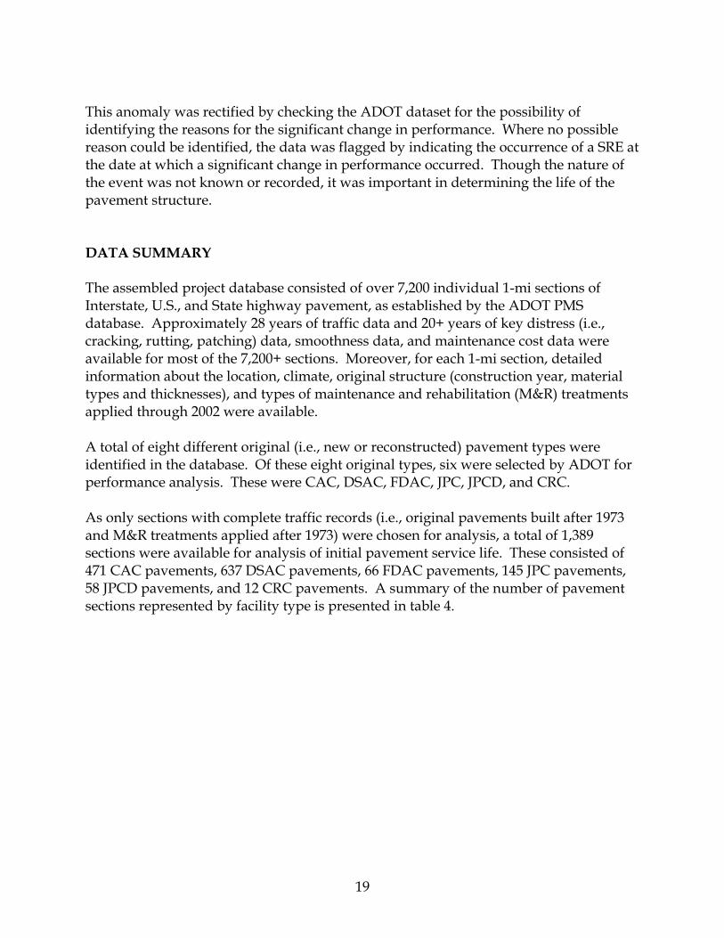
This anomaly was rectified by checking the ADOT dataset for the possibility of identifying the reasons for the significant change in performance. Where no possible reason could be identified, the data was flagged by indicating the occurrence of a SRE at the date at which a significant change in performance occurred. Though the nature of the event was not known or recorded, it was important in determining the life of the pavement structure. DATA SUMMARY The assembled project database consisted of over 7,200 individual 1-mi sections of Interstate, U.S., and State highway pavement, as established by the ADOT PMS database. Approximately 28 years of traffic data and 20+ years of key distress (i.e., cracking, rutting, patching) data, smoothness data, and maintenance cost data were available for most of the 7,200+ sections. Moreover, for each 1-mi section, detailed information about the location, climate, original structure (construction year, material types and thicknesses), and types of maintenance and rehabilitation (M&R) treatments applied through 2002 were available. A total of eight different original (i.e., new or reconstructed) pavement types were identified in the database. Of these eight original types, six were selected by ADOT for performance analysis. These were CAC, DSAC, FDAC, JPC, JPCD, and CRC. As only sections with complete traffic records (i.e., original pavements built after 1973 and M&R treatments applied after 1973) were chosen for analysis, a total of 1,389 sections were available for analysis of initial pavement service life. These consisted of 471 CAC pavements, 637 DSAC pavements, 66 FDAC pavements, 145 JPC pavements, 58 JPCD pavements, and 12 CRC pavements. A summary of the number of pavement sections represented by facility type is presented in table 4.

20
Table 4. Summary of the number of pavement sections along with facility types.
Pavement Type Facility Type No. of Sections Total
Interstates 121 State Routes 274 CAC
U.S. Highways 76 471
Interstates 318 State Routes 230 DSAC
U.S. Highways 89 637
Interstates 52 State Routes 14 FDAC
U.S. Highways 0 66
Interstates 25 State Routes 72 JPC
U.S. Highways 48 145
Interstates 54 State Routes 4 JPCD
U.S. Highways 0 58
Interstates 0 State Routes 12 CRC
U.S. Highways 0 12
Table 5 presents an overview of the ADOT Districts represented by the data used in analysis. For each District, the pavement sections were broken down by facility type (i.e., Interstate, U.S. highways, and State routes) and the following climatic zones, as defined by ADOT’s regional factor (RF):
• Hot-dry (RF≤1.5). • Moderate (1.5<RF≤3.0). • Cool-wet (RF>3.0).
The number of pavement sections per District ranged from 45 to 287. Depending on the geographic location of the District, all or some of the three climate types in Arizona were represented. Table 6 shows a breakdown of the pavement sections analyzed by highway. This table shows that the 1,389 pavement sections represent six different Interstates, eight different U.S. highways, and 38 different State routes. Although the State routes were well represented, their contribution in terms of actual pavement sections was limited, primarily because a high portion of them were originally constructed before 1973. A total of 570 pavement sections were located on Interstates, 606 were located on State routes, and the remaining 213 pavement sections were located on U.S. highways.

21
Table 5. Overview of the pavement sections used in analysis.
Facility Type ADOT District Climate Zone
Interstate State Routes U.S. Highways Total
Hot-Dry 86 133 53 Moderate 0 27 0 Phoenix Cool-Wet 0 0 0
299
Hot-Dry 42 9 2 Moderate 16 19 18 Flagstaff Cool-Wet 40 9 18
173
Hot-Dry 0 0 0 Moderate 0 25 9 Globe Cool-Wet 0 31 28
93
Hot-Dry 0 1 0 Moderate 25 11 8 Holbrook Cool-Wet 0 0 0
45
Hot-Dry 20 55 29 Moderate 142 13 7
Kingman
Cool-Wet 0 0 0
266
Hot-Dry 0 23 0 Moderate 21 68 0 Prescott Cool-Wet 0 45 0
157
Hot-Dry 0 0 0 Moderate 32 35 19 Safford Cool-Wet 0 0 0
86
Hot-Dry 0 44 0 Moderate 41 45 4 Tucson Cool-Wet 0 0 0
134
Hot-Dry 105 13 18 Moderate 0 0 0 Yuma Cool-Wet 0 0 0
136
22
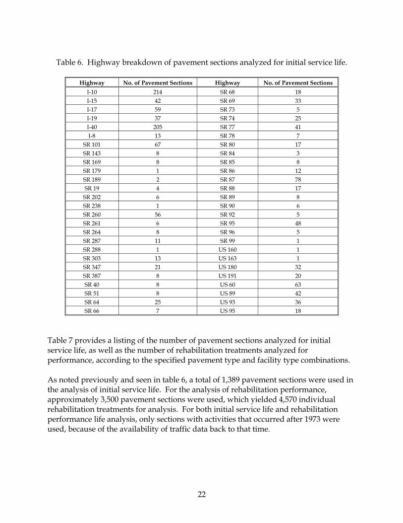
Table 6. Highway breakdown of pavement sections analyzed for initial service life.
Highway No. of Pavement Sections Highway No. of Pavement Sections
I-10 214 SR 68 18 I-15 42 SR 69 33 I-17 59 SR 73 5 I-19 37 SR 74 25 I-40 205 SR 77 41 I-8 13 SR 78 7
SR 101 67 SR 80 17 SR 143 8 SR 84 3 SR 169 8 SR 85 8 SR 179 1 SR 86 12 SR 189 2 SR 87 78 SR 19 4 SR 88 17
SR 202 6 SR 89 8 SR 238 1 SR 90 6 SR 260 56 SR 92 5 SR 261 6 SR 95 48 SR 264 8 SR 96 5 SR 287 11 SR 99 1 SR 288 1 US 160 1 SR 303 13 US 163 1 SR 347 21 US 180 32 SR 387 8 US 191 20 SR 40 8 US 60 63 SR 51 8 US 89 42 SR 64 25 US 93 36 SR 66 7 US 95 18
Table 7 provides a listing of the number of pavement sections analyzed for initial service life, as well as the number of rehabilitation treatments analyzed for performance, according to the specified pavement type and facility type combinations. As noted previously and seen in table 6, a total of 1,389 pavement sections were used in the analysis of initial service life. For the analysis of rehabilitation performance, approximately 3,500 pavement sections were used, which yielded 4,570 individual rehabilitation treatments for analysis. For both initial service life and rehabilitation performance life analysis, only sections with activities that occurred after 1973 were used, because of the availability of traffic data back to that time.

Table 7. Types of rehabilitation activities performed according to pavement and facility types. Original Construction/Reconstruction (O) and Rehabilitation (R) Groups O R1 R2 R3 R4 R5 R6 R7 R10 R12 R13
Pavement Type
Facility Type
Orig. Const.
& Reconst. a
HMA OL (1.5”<T≤4.0”)
b
HMA OL (T>4.0”) b
Shallow Mill (<4.0”) & HMA OL
(1.5”<T≤4.0”) b
Shallow Mill
(<4.0”) & HMA OL (T>4.0”) b
Deep Mill (>4.0”) & HMA OL
(1.5”<T≤4.0”) b
Deep Mill (>4.0”) & HMA OL (T>4.0”) b
Diamond Grind
Restoration & HMA OL
(1.5”<T≤4.0”) b
Crack/Seat & HMA OL
(1.5”<T≤4.0”) b
Crack/Seat & HMA OL
(T>4.0”) b
Interstates 121 356 131 453 822 1 268 0 0 0 0 State Routes 274 907 54 123 59 0 10 0 0 0 0 CAC
U.S. Routes 76 686 36 133 99 0 7 0 0 0 0 Interstates 318 3 4 82 78 7 75 0 0 0 0
State Routes 230 43 0 19 0 0 2 0 0 0 0 DSAC
U.S. Routes 89 1 0 0 0 0 0 0 0 0 0 Interstates 52 0 4 32 0 0 25 0 0 0 0
State Routes 14 1 0 0 1 0 0 0 0 0 0
FDAC
U.S. Routes 0 0 0 0 0 0 0 0 0 0 0 Interstates 25 33 15 23 0 0 0 50 25 14 9
State Routes 72 7 0 0 0 0 0 0 0 0 0 JPC
U.S. Routes 48 0 0 0 0 0 0 0 0 0 0 Interstates 54 0 0 0 0 0 0 0 0 0 0
State Routes 4 0 0 0 0 0 0 0 0 0 0 JPCD
U.S. Routes 0 0 0 0 0 0 0 0 0 0 0 Interstates 0 0 0 0 0 0 0 0 0 0 0
State Routes 12 0 0 0 0 0 0 0 0 0 0 CRC
U.S. Routes 0 0 0 0 0 0 0 0 0 0 0
TOTAL 1,389 2,037 244 865 1,059 8 387 50 25 14 9 a Based on pavement sections originally constructed or reconstructed after 1973. b Based on rehabilitation treatments that occurred after 1973. T = Thickness. OL = Overlay.
23

24
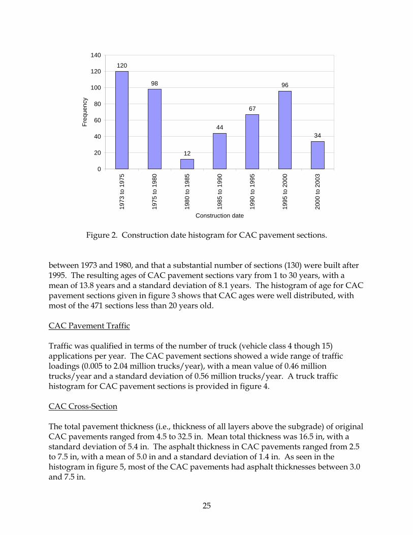
Descriptive Statistics for CAC Pavements The project database contains a variety of data elements for 471 CAC pavement sections built (constructed or reconstructed) after 1973. A breakdown of the CAC pavement sections among the nine ADOT Districts and three climatic regions is provided in table 8. As can be seen, each District and climate is represented, though it should be noted that the distribution of climate zones within a District is limited by the geographic location of the District. CAC Construction Year and Age The histogram in figure 2 shows the distribution of construction dates for CAC pavements. It can be seen that most of the sections analyzed (218 out of 471) were built
Table 8. Location breakdown of CAC pavement sections.
ADOT District Climate Number of Pavement Sections Hot-Dry 32
Moderate 19 Phoenix
Cool-Wet 0 Hot-Dry 20
Moderate 10 Flagstaff Cool-Wet 16 Hot-Dry 0
Moderate 20 Globe Cool-Wet 22 Hot-Dry 1
Moderate 13 Holbrook Cool-Wet 0 Hot-Dry 58
Moderate 33 Kingman Cool-Wet 0 Hot-Dry 22
Moderate 34 Prescott Cool-Wet 26 Hot-Dry 0
Moderate 23 Safford Cool-Wet 0 Hot-Dry 34
Moderate 15 Tucson Cool-Wet 0 Hot-Dry 72
Moderate 0 Yuma Cool-Wet 0
25
Figure 2. Construction date histogram for CAC pavement sections. between 1973 and 1980, and that a substantial number of sections (130) were built after 1995. The resulting ages of CAC pavement sections vary from 1 to 30 years, with a mean of 13.8 years and a standard deviation of 8.1 years. The histogram of age for CAC pavement sections given in figure 3 shows that CAC ages were well distributed, with most of the 471 sections less than 20 years old. CAC Pavement Traffic Traffic was qualified in terms of the number of truck (vehicle class 4 though 15) applications per year. The CAC pavement sections showed a wide range of traffic loadings (0.005 to 2.04 million trucks/year), with a mean value of 0.46 million trucks/year and a standard deviation of 0.56 million trucks/year. A truck traffic histogram for CAC pavement sections is provided in figure 4. CAC Cross-Section The total pavement thickness (i.e., thickness of all layers above the subgrade) of original CAC pavements ranged from 4.5 to 32.5 in. Mean total thickness was 16.5 in, with a standard deviation of 5.4 in. The asphalt thickness in CAC pavements ranged from 2.5 to 7.5 in, with a mean of 5.0 in and a standard deviation of 1.4 in. As seen in the histogram in figure 5, most of the CAC pavements had asphalt thicknesses between 3.0 and 7.5 in.
120
98
12
44
67
96
34
0
20
40
60
80
100
120
140
1973
to 1
975
1975
to 1
980
1980
to 1
985
1985
to 1
990
1990
to 1
995
1995
to 2
000
2000
to 2
003
Construction date
Freq
uenc
y

26
Figure 3. Age histogram for CAC pavement sections.
Figure 4. Traffic histogram for CAC pavement sections.
7480
91
128
25
73
0
20
40
60
80
100
120
140
< 5
5 to
10
10 to
15
15 to
20
20 to
25
25 to
30
Age, years
Freq
uenc
y
319
98
24 16 14
0
50
100
150
200
250
300
350
0 to
0.5
0.5
to 1
.0
1 to
1.5
1.5
to 2
.0
2 to
2.5
Trucks/year (millions)
Freq
uenc
y

27
Figure 5. Asphalt thickness histogram for CAC pavement sections. Descriptive Statistics for DSAC Pavements The project database contains a variety of data elements for 637 DSAC pavement sections built (constructed or reconstructed) after 1973. As seen in table 9, all nine ADOT Districts and all three climatic zones were represented by DSAC pavements. DSAC Construction Year and Age The construction date histogram in figure 6 shows that 356 out of the 637 DSAC sections analyzed were constructed between 1973 and 1980, while 145 were constructed between 1990 and 1995. Forty-seven pavement sections were constructed between 1980 and 1985. The resulting ages of DSAC pavement sections ranged from 1 to 30 years, with a mean of 16.0 years and a standard deviation of 6.7 years. As seen by the age histogram in figure 7, the DSAC pavement ages were well distributed with most of the 637 sections between 10 and 25 years old.
82
65
91
130
103
0
20
40
60
80
100
120
140
2.5
to 3
.5
3.5
to 4
.5
4.5
to 5
.5
5.5
to 6
.5
6.5
to 7
.5
Surface Thickness, in
Freq
uenc
y
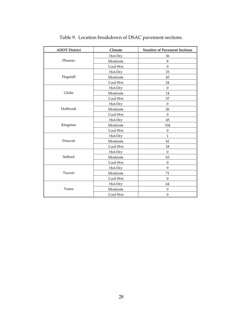
28
Table 9. Location breakdown of DSAC pavement sections.
ADOT District Climate Number of Pavement Sections
Hot-Dry 36 Moderate 8 Phoenix
Cool-Wet 0 Hot-Dry 33
Moderate 43 Flagstaff Cool-Wet 24 Hot-Dry 0
Moderate 14 Globe Cool-Wet 37 Hot-Dry 0
Moderate 26 Holbrook Cool-Wet 0 Hot-Dry 45
Moderate 104 Kingman Cool-Wet 0 Hot-Dry 1
Moderate 41 Prescott Cool-Wet 18 Hot-Dry 0
Moderate 63 Safford Cool-Wet 0 Hot-Dry 9
Moderate 71 Tucson Cool-Wet 0 Hot-Dry 64
Moderate 0 Yuma Cool-Wet 0

29
Figure 6. Construction date histogram for DSAC pavement sections.
Figure 7. Age histogram for DSAC pavement sections.
96
260
47 45
145
23 21
0
50
100
150
200
250
300
1973
to 1
975
1975
to 1
980
1980
to 1
985
1985
to 1
990
1990
to 1
995
1995
to 2
000
2000
to 2
003
Construction date
Freq
uenc
y
4233
203
155137
67
0
50
100
150
200
250
< 5
5 to
10
10 to
15
15 to
20
20 to
25
25 to
30
Age, years
Freq
uenc
y
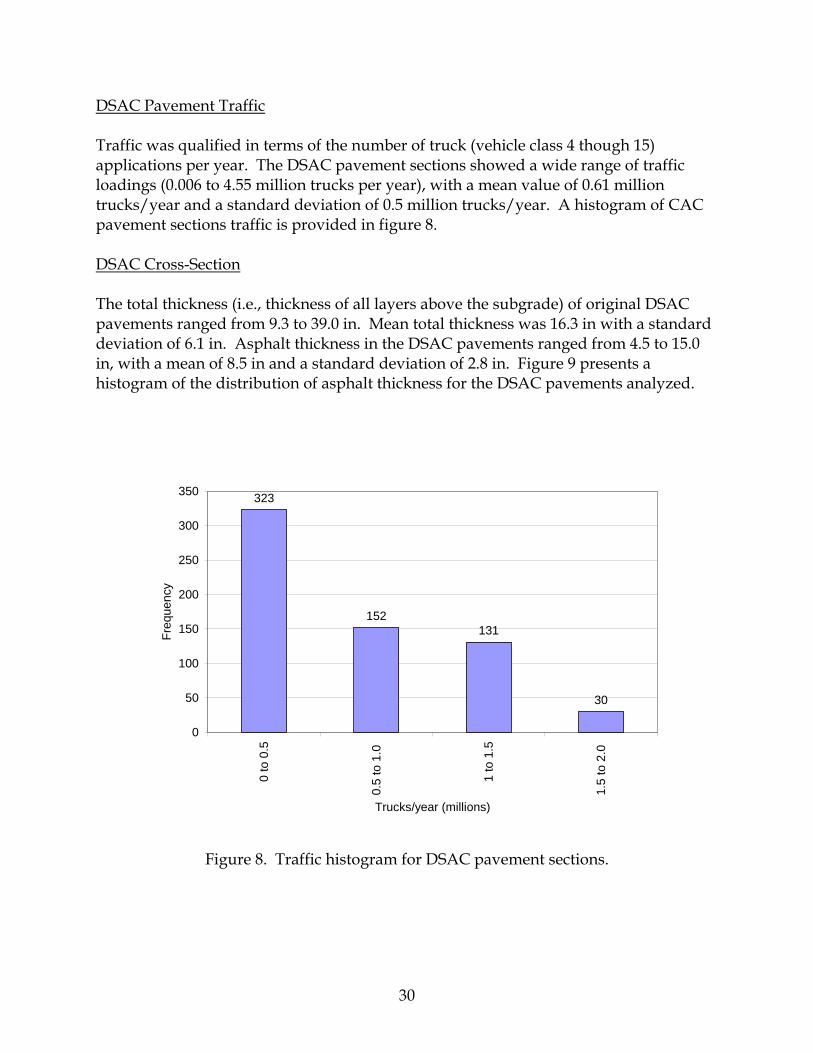
30
DSAC Pavement Traffic Traffic was qualified in terms of the number of truck (vehicle class 4 though 15) applications per year. The DSAC pavement sections showed a wide range of traffic loadings (0.006 to 4.55 million trucks per year), with a mean value of 0.61 million trucks/year and a standard deviation of 0.5 million trucks/year. A histogram of CAC pavement sections traffic is provided in figure 8. DSAC Cross-Section The total thickness (i.e., thickness of all layers above the subgrade) of original DSAC pavements ranged from 9.3 to 39.0 in. Mean total thickness was 16.3 in with a standard deviation of 6.1 in. Asphalt thickness in the DSAC pavements ranged from 4.5 to 15.0 in, with a mean of 8.5 in and a standard deviation of 2.8 in. Figure 9 presents a histogram of the distribution of asphalt thickness for the DSAC pavements analyzed.
Figure 8. Traffic histogram for DSAC pavement sections.
323
152131
30
0
50
100
150
200
250
300
350
0 to
0.5
0.5
to 1
.0
1 to
1.5
1.5
to 2
.0
Trucks/year (millions)
Freq
uenc
y

31
Figure 9. Asphalt thickness histogram for DSAC pavement sections. Descriptive Statistics for FDAC Pavements The project database contains a variety of data elements for 66 FDAC pavement sections constructed or reconstructed after 1973. Table 10 shows the breakdown of FDAC sections among the nine ADOT Districts and three climatic regions. As can be seen, four Districts and all three climates were represented, though most sections fell within the hot-dry and moderate climates. FDAC Construction Year and Age The construction date histogram in figure 10 shows that most of the FDAC sections analyzed (53 out of 66) were constructed between 1975 and 1980. Only four were built after 1985 and none were built after 1989. The resulting ages of FDAC pavement sections ranged from 1 to 23 years, with a mean of 16.7 years and a standard deviation of 5.8 years. As seen in the age histogram in figure 11 the vast majority of sections were between 15 and 25 years old.
89 88
55
87
99
33
70
38
52
0
26
0
20
40
60
80
100
120
4.5
to 5
.5
5.5
to 6
.5
6.5
to 7
.5
7.5
to 8
.5
8.5
to 9
.5
9.5
to 1
0.5
10.5
to 1
1.5
11.5
to 1
2.5
12.5
to 1
3.5
13.5
to 1
4.5
14.5
to 1
5.5
Surface Thickness, in
Freq
uenc
y

32
Table 10. Location breakdown of FDAC pavement sections.
ADOT District Climate Number of Pavement Sections
Hot-Dry 21 Moderate 0 Phoenix
Cool-Wet 0 Hot-Dry 0
Moderate 5 Holbrook Cool-Wet 0 Hot-Dry 0
Moderate 25 Kingman Cool-Wet 0 Hot-Dry 0
Moderate 14 Prescott Cool-Wet 1
Figure 10. Construction date histogram for FDAC pavement sections.
0
53
94
0 0 00
10
20
30
40
50
60
1973
to 1
975
1975
to 1
980
1980
to 1
985
1985
to 1
990
1990
to 1
995
1995
to 2
000
2000
to 2
003
Construction date
Freq
uenc
y

33
Figure 11. Age histogram for FDAC pavement sections. FDAC Pavement Traffic Traffic was qualified in terms of the number of truck (vehicle class 4 though 15) applications per year. The FDAC pavement sections showed a wide range of traffic loading (0.05 to 1.6 million trucks/year), with a mean value of 0.8 million trucks/year and a standard deviation of 0.4 million trucks/year. A histogram of truck traffic for FDAC pavements is provided in figure 12. FDAC Cross-Section The total thickness (i.e., thickness of all layers above the subgrade) of original FDAC pavements ranged from 8.5 to 24.5 in. Mean total thickness was 15.6 in, with a standard deviation of 5.9 in. The asphalt thickness of FDAC pavements ranged from 3.0 to 12.5 in, with a mean of 7.7 in and a standard deviation of 2.9 in. The histogram in figure 13 shows that most of the FDAC pavements had an asphalt thickness between 4.5 and 11.0 in.
5
1
7
21
32
00
5
10
15
20
25
30
35
< 5
5 to
10
10 to
15
15 to
20
20 to
25
25 to
30
Age, years
Freq
uenc
y

34
Figure 12. Traffic histogram for FDAC pavement sections.
Figure 13. Asphalt thickness histogram for FDAC pavement sections.
14
35
15
2
0
5
10
15
20
25
30
35
40
0 to
0.5
0.5
to 1
.0
1 to
1.5
1.5
to 2
.0
Trucks/year (millions)
Freq
uenc
y
4 4
10 11
3 2 24
26
0
5
10
15
20
25
30
2.5
to 3
.5
3.5
to 4
.5
4.5
to 5
.5
5.5
to 6
.5
6.5
to 7
.5
7.5
to 8
.5
8.5
to 9
.5
9.5
to 1
0.5
10.5
to 1
1.5
Surface Thickness, in
Freq
uenc
y

35
Descriptive Statistics for JPC Pavements The project database contains a variety of data elements for 145 JPC pavement sections constructed or reconstructed after 1973. As seen in table 11, the JPC pavement sections analyzed were located in four of the nine ADOT Districts and in the hot-dry and cool-wet climatic regions. JPC Pavement Age The histogram in figure 14 shows the distribution of construction dates for JPC pavements. Most of the sections in the 1973 to 1979 category were built in the Flagstaff District, whereas most of those built between 1995 and 2003 were located in the Phoenix District. The resulting ages of JPC pavement sections ranged from 1 to 28 years, with a mean of 11.4 years and a standard deviation of 7.3 years. The histogram in figure 15 shows more than half of the JPC sections used in analysis were less than 15 years old. JPC Pavement Traffic Traffic was qualified in terms of the number of truck (vehicle class 4 though 15) applications per year. The JPC pavement sections showed a wide range of traffic loading (0.05 to 2.6 million trucks/year), with a mean value of 0.87 million trucks/year and a standard deviation of 0.54 million trucks/year. A histogram showing the annual truck traffic for JPC pavements is provided in figure 16. PCC Slab Thickness The total pavement thickness (i.e., thickness of all layers above the subgrade) of original JPC pavement sections ranged from 10.0 to 20.0 in. Mean total thickness was 16.2 in, with a standard deviation of 2.3 in. PCC surface thickness for the JPC pavements ranged from 8.0 to 16.0 in, with a mean of 11.2 in and a standard deviation of 2.15 in. The histogram in figure 17 shows that most of the JPC pavements analyzed had slab thicknesses between 7.5 and 13.5 in.
Table 11. Location breakdown of JPC pavement sections. ADOT District Climate Number of Pavement Sections
Hot-Dry 117 Moderate 0 Phoenix
Cool-Wet 0 Hot-Dry 0
Moderate 0 Flagstaff Cool-Wet 27 Hot-Dry 1
Moderate 0 Tucson Cool-Wet 0

36
Figure 14. Construction date histogram for JPC pavements.
Figure 15. Age histogram for JPC pavement sections.
14
21
810
39
2825
0
5
10
15
20
25
30
35
40
45
1973
to 1
975
1975
to 1
980
1980
to 1
985
1985
to 1
990
1990
to 1
995
1995
to 2
000
2000
to 2
003
Construction date
Freq
uenc
y
41
12
42
23 24
3
0
5
10
15
20
25
30
35
40
45
< 5
5 to
10
10 to
15
15 to
20
20 to
25
25 to
30
Age, years
Freq
uenc
y

37
Figure 16. Traffic histogram for JPC pavement sections.
Figure 17. Slab thickness histogram for JPC pavement sections.
39
63
22
13
62
0
10
20
30
40
50
60
70
0 to
0.5
0.5
to 1
.0
1 to
1.5
1.5
to 2
.0
2 to
2.5
2.5
to 3
.0
Trucks/year (millions)
Freq
uenc
y
1 0
25
17
2
23
29
38
24 4
0
5
10
15
20
25
30
35
40
5.5
to 6
.5
6.5
to 7
.5
7.5
to 8
.5
8.5
to 9
.5
9.5
to 1
0.5
10.5
to 1
1.5
11.5
to 1
2.5
12.5
to 1
3.5
13.5
to 1
4.5
14.5
to 1
5.5
15.5
to 1
6.0
Surface PCC Thickness, in
Freq
uenc
y

38
Descriptive Statistics for JPCD Pavements The project database contains a variety of data elements for 58 JPCD pavement sections constructed or reconstructed after 1973. As table 12 shows, the JPCD pavement sections analyzed were located in the Phoenix and Tucson Districts and in the hot-dry and moderate climates. JPCD Construction Year and Age The histogram in figure 18 shows the distribution of construction dates for JPCD pavements. It can be seen in this figure that all of the sections analyzed were built after 1980. The resulting ages of JPCD pavement sections ranged from 2 to 19 years, with a mean of 12.9 years and a standard deviation of 5.5 years. The age histogram in figure 19 shows that most JPCD pavement sections were less than 20 years old. JPCD Pavement Traffic Traffic was qualified in terms of the number of truck (vehicle class 4 though 15) applications per year. The JPCD pavement sections showed a very wide range of traffic loadings (0.9 to 6.7 million trucks/year), with a mean value of 3.8 million trucks/year and a standard deviation of 1.7 million trucks/year. A traffic histogram of JPCD pavement sections is provided in figure 20. PCC Slab Thickness The total thickness (i.e., thickness of all layers above the subgrade) of original JPCD pavement sections ranged from 15.0 to 29.0 in. Mean total thickness was 16.5 in, with a standard deviation of 3.5 in. PCC surface thickness ranged from 10.0 to 15.0 in, with a mean of 11.3 in and a standard deviation of 1.71 in. The histogram in figure 21 shows the distribution of PCC thickness for the JPCD pavements analyzed.
Table 12. Location breakdown of JPCD pavement sections.
ADOT District Climate Number of Pavement Sections
Hot-Dry 54 Moderate 0 Phoenix
Cool-Wet 0 Hot-Dry 0
Moderate 4 Tucson Cool-Wet 0
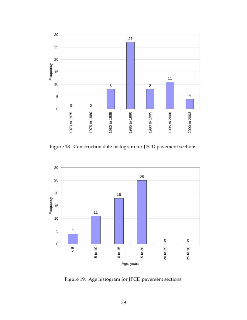
39
Figure 18. Construction date histogram for JPCD pavement sections.
Figure 19. Age histogram for JPCD pavement sections.
0 0
8
27
8
11
4
0
5
10
15
20
25
30
1973
to 1
975
1975
to 1
980
1980
to 1
985
1985
to 1
990
1990
to 1
995
1995
to 2
000
2000
to 2
003
Freq
uenc
y
4
11
18
25
0 00
5
10
15
20
25
30
< 5
5 to
10
10 to
15
15 to
20
20 to
25
25 to
30
Age, years
Freq
uenc
y

40
Figure 20. Traffic histogram for JPCD pavement sections.
Figure 21. Slab thickness histogram for JPCD pavement sections.
43 3
56
2
8
2
6
910
0
2
4
6
8
10
12
0.5
to 1
.0
1 to
1.5
1.5
to 2
.0
2 to
2.5
2.5
to 3
.0
3 to
3.5
3.5
to 4
.0
4 to
4.5
4.5
to 5
.0
5 to
5.5
5.5
to 6
.0
Trucks/year (millions)
Freq
uenc
y
35
0
4
11
4 4
0
5
10
15
20
25
30
35
40
9.5
to 1
0.5
10.5
to 1
1.5
11.5
to 1
2.5
12.5
to 1
3.5
13.5
to 1
4.5
14.5
to 1
5.5
Surface PCC Thickness, in
Freq
uenc
y
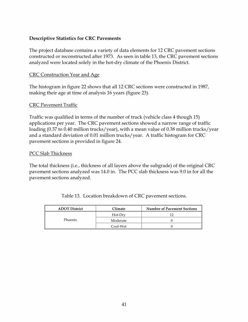
41
Descriptive Statistics for CRC Pavements The project database contains a variety of data elements for 12 CRC pavement sections constructed or reconstructed after 1973. As seen in table 13, the CRC pavement sections analyzed were located solely in the hot-dry climate of the Phoenix District. CRC Construction Year and Age The histogram in figure 22 shows that all 12 CRC sections were constructed in 1987, making their age at time of analysis 16 years (figure 23). CRC Pavement Traffic Traffic was qualified in terms of the number of truck (vehicle class 4 though 15) applications per year. The CRC pavement sections showed a narrow range of traffic loading (0.37 to 0.40 million trucks/year), with a mean value of 0.38 million trucks/year and a standard deviation of 0.01 million trucks/year. A traffic histogram for CRC pavement sections is provided in figure 24. PCC Slab Thickness The total thickness (i.e., thickness of all layers above the subgrade) of the original CRC pavement sections analyzed was 14.0 in. The PCC slab thickness was 9.0 in for all the pavement sections analyzed.
Table 13. Location breakdown of CRC pavement sections.
ADOT District Climate Number of Pavement Sections Hot-Dry 12
Moderate 0 Phoenix
Cool-Wet 0
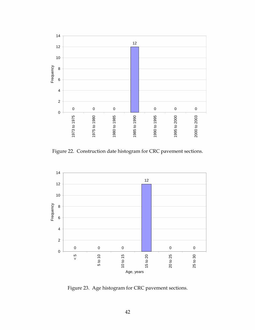
42
Figure 22. Construction date histogram for CRC pavement sections.
Figure 23. Age histogram for CRC pavement sections.
0 0 0
12
0 0 00
2
4
6
8
10
12
14
1973
to 1
975
1975
to 1
980
1980
to 1
985
1985
to 1
990
1990
to 1
995
1995
to 2
000
2000
to 2
003
Freq
uenc
y
0 0 0
12
0 00
2
4
6
8
10
12
14
< 5
5 to
10
10 to
15
15 to
20
20 to
25
25 to
30
Age, years
Freq
uenc
y
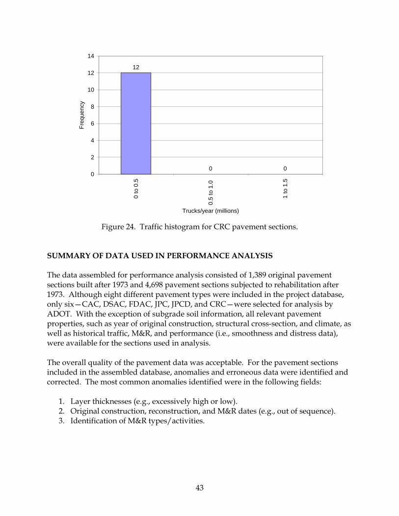
43
Figure 24. Traffic histogram for CRC pavement sections. SUMMARY OF DATA USED IN PERFORMANCE ANALYSIS The data assembled for performance analysis consisted of 1,389 original pavement sections built after 1973 and 4,698 pavement sections subjected to rehabilitation after 1973. Although eight different pavement types were included in the project database, only six—CAC, DSAC, FDAC, JPC, JPCD, and CRC—were selected for analysis by ADOT. With the exception of subgrade soil information, all relevant pavement properties, such as year of original construction, structural cross-section, and climate, as well as historical traffic, M&R, and performance (i.e., smoothness and distress data), were available for the sections used in analysis. The overall quality of the pavement data was acceptable. For the pavement sections included in the assembled database, anomalies and erroneous data were identified and corrected. The most common anomalies identified were in the following fields:
1. Layer thicknesses (e.g., excessively high or low). 2. Original construction, reconstruction, and M&R dates (e.g., out of sequence). 3. Identification of M&R types/activities.
12
0 00
2
4
6
8
10
12
14
0 to
0.5
0.5
to 1
.0
1 to
1.5
Trucks/year (millions)
Freq
uenc
y

44
These anomalies were rectified by:
• Reviewing the ADOT database for additional information (construction history, M&R, and so on.
• Reviewing similar information available for adjacent pavement sections. • Conducting interviews with or sending feedback information to relevant ADOT
personnel. Where the correct information could be found, the anomalous data were corrected or replaced. Otherwise, the section was removed from the database and not used in the analysis. Data points deemed to be outliers or erroneous were also removed from the database. Over 7,200 pavement sections were available in the ADOT PMS database. Approximately 20 percent (1,389 of 7,200) were included in the analysis of new/reconstructed pavements, while approximately 65 percent (4,698 of 7,200) were included in the analysis of pavement rehabilitation. The pavement sections included adequately represented the data available in the ADOT database and the population of pavements available in Arizona. Pavement sections not included in the samples for analysis did not have all the required data available. Table 14 presents a summary of the pavement section included in the databases for analysis. As can be seen, there was generally sufficient data available for analysis and decision-making for CAC, DSAC, and FDAC pavements. However, the data available for PCC pavements (JPC, JPCD, and CRC) was somewhat limited. There was no data available for the rehabilitation of JPCD and CRC, thereby limiting the ability to reasonably estimate the performance of rehabilitation treatments on these pavement types.
Table 14. Summary of pavement sections included in databases for analysis.
Total Number of Sections Pavement Type New and Reconstructed Rehabilitation
CAC 471 4,145 DSAC and FDAC 703 377 JPC 145 176 JPCD 58 0 CRC 12 0
Summary Descriptive Statistics for Asphalt-Surfaced Pavements A summary of the descriptive statistics for asphalt-surfaced pavements used in the analysis of initial pavement life is provided in figures 25 through 27. These figures show a good representation of current asphalt pavement design practices and the expected traffic loadings for each asphalt pavement type.
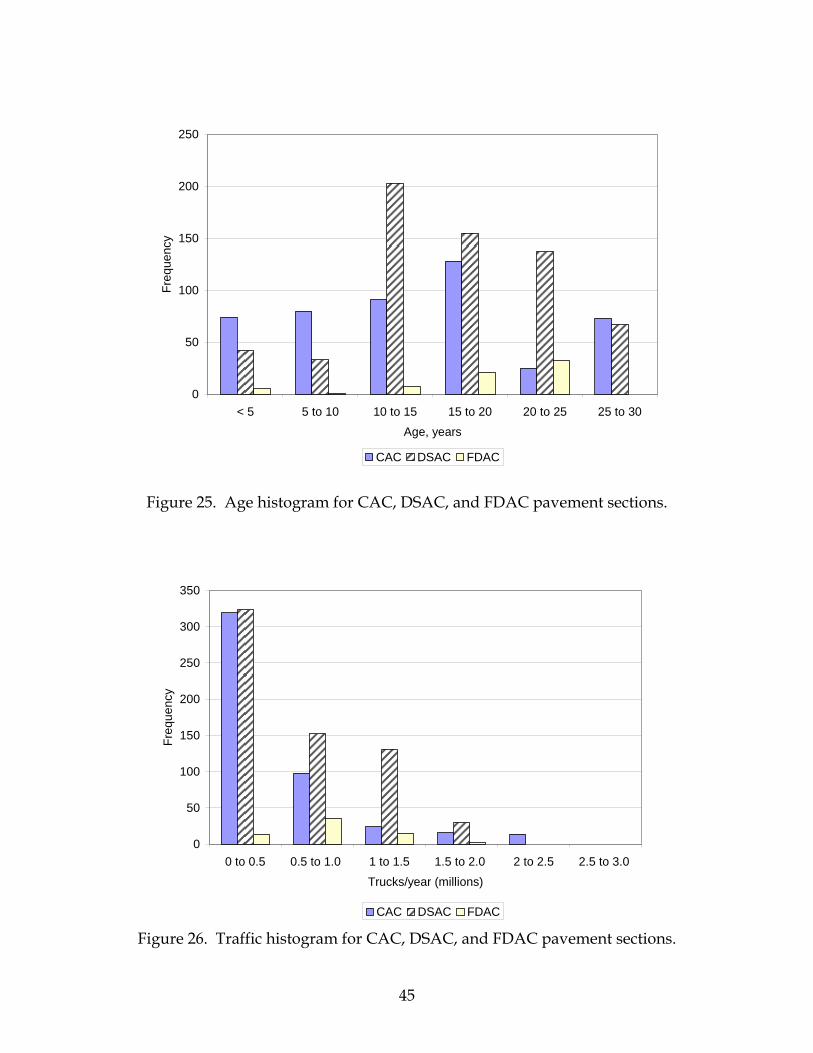
45
Figure 25. Age histogram for CAC, DSAC, and FDAC pavement sections.
Figure 26. Traffic histogram for CAC, DSAC, and FDAC pavement sections.
0
50
100
150
200
250
< 5 5 to 10 10 to 15 15 to 20 20 to 25 25 to 30Age, years
Freq
uenc
y
CAC DSAC FDAC
0
50
100
150
200
250
300
350
0 to 0.5 0.5 to 1.0 1 to 1.5 1.5 to 2.0 2 to 2.5 2.5 to 3.0 Trucks/year (millions)
Freq
uenc
y
CAC DSAC FDAC

46
Figure 27. Asphalt thickness histogram for CAC, DSAC, and FDAC pavement sections. Summary Descriptive Statistics for PCC-Surfaced Pavements A summary of the descriptive statistics for PCC-surfaced pavements used in the analysis of initial pavement life is provided in figures 28 through 30. These figures show a good representation of current concrete pavement design practices and the expected traffic loadings for each type of PCC pavement.
0
20
40
60
80
100
120
140
2.5to3.5
3.5to4.5
4.5to5.5
5.5to6.5
6.5to7.5
7.5to8.5
8.5to
9.5
9.5to
10.5
10.5to
11.5
11.5to
12.5
12.5to
13.5
13.5to
14.5
14.5to
15.5
15.5to
16.0
Surface Thickness, in
Freq
uenc
y
CAC DSAC FDAC
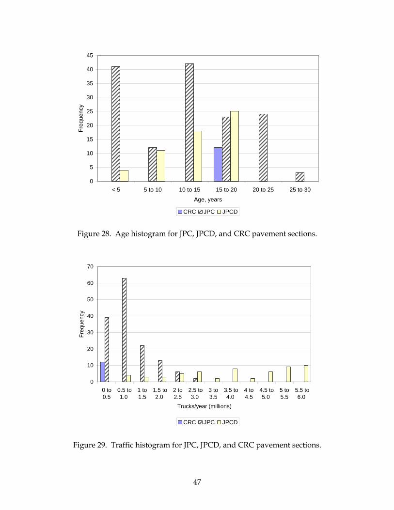
47
Figure 28. Age histogram for JPC, JPCD, and CRC pavement sections.
Figure 29. Traffic histogram for JPC, JPCD, and CRC pavement sections.
0
5
10
15
20
25
30
35
40
45
< 5 5 to 10 10 to 15 15 to 20 20 to 25 25 to 30
Age, years
Freq
uenc
y
CRC JPC JPCD
0
10
20
30
40
50
60
70
0 to0.5
0.5 to1.0
1 to1.5
1.5 to2.0
2 to2.5
2.5 to3.0
3 to3.5
3.5 to4.0
4 to4.5
4.5 to5.0
5 to5.5
5.5 to6.0
Trucks/year (millions)
Freq
uenc
y
CRC JPC JPCD

48
Figure 30. Slab thickness histogram for JPC, JPCD, and CRC pavement sections.
0
5
10
15
20
25
30
35
40
7.5
to 8
.5
8.5
to 9
.5
9.5
to 1
0.5
10.5
to 1
1.5
11.5
to 1
2.5
12.5
to 1
3.5
13.5
to 1
4.5
14.5
to 1
5.5
15.5
to 1
6.0
Surface Thickness, in
Freq
uenc
y
CRC JPC JPCD

49
CHAPTER 3. PAVEMENT PERFORMANCE ANALYSIS INTRODUCTION Survival analysis and mechanistic-based performance evaluation methods were used to analyze and develop estimates of (a) the service lives of newly constructed or reconstructed flexible and rigid pavements, and (b) the performance of rehabilitation treatments, as delineated by the categories listed in tables 2 and 3 in chapter 2. The pavement performance analysis consisted of the following steps:
1. Using the databases assembled as part of this study and described previously in chapter 2, establish analysis cells based on factors known to affect pavement life (these factors were determined based on engineering judgment).
2. Develop survival functions and determine estimated service lives for newly constructed or reconstructed flexible and rigid pavements for each of the analysis cells established.
3. Revise the analysis cells to reflect (a) data availability and (b) similarity in service life estimates.
4. Develop survival functions and determine service lives for rehabilitation treatments placed on original flexible and rigid pavements, in accordance with the revised analysis cells.
5. Conduct additional performance analyses using mechanistic–empirical (M–E) models developed as part of NCHRP Project 1-37A; the objective being to confirm original service life estimates from the survival analysis (for analysis cells with adequate or inadequate levels of data available) and/or to estimate initial life for analysis cells with no or very limited data.
PAVEMENT SURVIVAL ANALYSIS The statistical tool used for determining the expected service life of pavements and the performance of rehabilitation treatments was survival analysis. Survival analysis techniques have been widely and successfully applied in social sciences, economics, and engineering (reliability and failure time analysis). Specifically, for pavement engineering, survival analysis has been used for studying the effect of factors such as site conditions, design features, construction techniques, maintenance treatments, and rehabilitation activities on pavement service life. Pavement service life is the period of time over which no major cost events (i.e., rehabilitation, reconstruction) are required in providing a reasonable level of service to users. It must be noted that level of service is not a technical term and depends on the users and/or owners expectations of performance and service. Thus, it may differ from the pavement’s economic life, physical life, or design life.
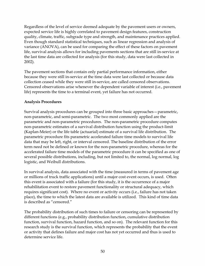
50
Regardless of the level of service deemed adequate by the pavement users or owners, expected service life is highly correlated to pavement design features, construction quality, climate, traffic, subgrade type and strength, and maintenance practices applied. Even though standard statistical techniques, such as linear regression and analysis of variance (ANOVA), can be used for comparing the effect of these factors on pavement life, survival analysis allows for including pavements sections that are still in-service at the last time data are collected for analysis (for this study, data were last collected in 2002). The pavement sections that contain only partial performance information, either because they were still in-service at the time data were last collected or because data collection ceased while they were still in-service, are called censored observations. Censored observations arise whenever the dependent variable of interest (i.e., pavement life) represents the time to a terminal event, yet failure has not occurred. Analysis Procedures Survival analysis procedures can be grouped into three basic approaches—parametric, non-parametric, and semi-parametric. The two most commonly applied are the parametric and non-parametric procedures. The non-parametric procedure computes non-parametric estimates of a survival distribution function using the product-limit (Kaplan-Meier) or the life table (actuarial) estimate of a survival life distribution. The parametric procedure fits parametric accelerated failure time models to survival life data that may be left, right, or interval censored. The baseline distribution of the error term need not be defined or known for the non-parametric procedure, whereas for the accelerated failure time models of the parametric procedure it can be specified as one of several possible distributions, including, but not limited to, the normal, log normal, log logistic, and Weibull distributions. In survival analysis, data associated with the time (measured in terms of pavement age or millions of truck traffic applications) until a major cost event occurs, is used. Often this event is associated with a failure (for this study, it is the occurrence of a major rehabilitation event to restore pavement functionality or structural adequacy, which requires significant cost). Where no event or activity occurs (i.e., failure has not taken place), the time to which the latest data are available is utilized. This kind of time data is described as “censored.” The probability distribution of such times to failure or censoring can be represented by different functions (e.g., probability distribution function, cumulative distribution function, survival function, hazard function, and so on). The relevant function for this research study is the survival function, which represents the probability that the event or activity that defines failure and major cost has not yet occurred and thus is used to determine service life.

51
Therefore, for both the non-parametric and parametric procedures, the first step in determining expected pavement service life is defining the survival function. The survival function, conventionally denoted by S, is defined as follows: S(t) = Pr(T>t) Eq. 1 where: t = Time or age of pavement (or cumulative number of truck loadings). T = Time or age of pavement at failure (or cumulative number of truck
loadings at failure. Pr = Probability. Hence, the survival function is the probability that pavement time to failure (measured in terms of age [years] or cumulative traffic [number of truck applications]) is greater than some specified age or truck application level. For continuous probability distribution functions, equation 1 is modified and the survival function is defined as follows: Eq. 2 where: f(t) = Probability distribution function (pdf). F(t) = Cumulative density function (cdf) of the given distribution (e.g.,
normal, log logistic, Wiebull). The survival function has the following characteristics:
1. It assumes that S(0) = 1 (although it could be less than 1 if there is the possibility of immediate pavement failure due to construction error).
2. Survival probability decreases with increasing life (i.e., S(u) < S(t) if u > t). This expresses the notion that survival is only less probable as the pavement ages or as more trucks are applied to the pavement.
3. Survival probability is usually assumed to approach zero as pavement age or traffic applications increases without bound (i.e., S(t) → 0 as t [measured as pavement age of the number of truck applications] → ∞).
Both the parametric and non-parametric procedures were applied in this study for estimating pavement service life. Brief descriptions of the two procedures are presented in the sections below. Non-Parametric Procedure (LIFETEST) The most straightforward survival analysis procedure is the non-parametric procedure. In this procedure, life tables are used to calculate various types of time-to-failure distributions, such as the survival function, hazard functions, and so on. These life
∫∞
−==t
tFdTTfts )(1)()(
52
tables can be thought of as an "enhanced" frequency distribution table. The distribution of survival times is divided into a given number of intervals. For each interval the following items are computed:
1. The number and proportion of pavements that entered the respective interval in “good condition."
2. The number and proportion of pavements that failed in the respective interval (i.e., number of terminal events, or number of pavements that were “subjected to major rehabilitation or reconstruction").
3. The number of pavements with no data (unfailed) available (i.e., censored in the respective interval).
Using the computations listed above, a life table can be populated. Examples of information contained in a life table are as follows:
• Number of pavements at risk (pavements yet to fail). • Proportion of pavements that have failed. • Proportion of pavements that have survived. • Cumulative proportion surviving or failing (survival function). • Median survival time and/or traffic.
These statistics form the basis for determining the service life at which the cumulative survival function is equal to a given percentile (e.g., 25th, 50th, and 75th percentile). (It should be noted that the 50th percentile, or median, for the cumulative survival function is usually not the same as the point in time up to which 50 percent of the sample survived. This would only be the case if there were no censored observations prior to this time). Life tables are developed based on the following assumptions:
• For a given population of pavements, the exact service life of each pavement is independent and identically distributed. (Note that since the life table procedure is a non-parametric procedure, knowledge of the specific failure time distribution [e.g., normal, Weibull, and so on] is not required. However, it is essential that all the survival functions follow the same distribution).
• The pavement sections are a random sample from the population of interest and thus they are independent of each other and unbiased.
• If any pavement sections are censored, they must be randomly censored, and the distribution of censoring times is independent of the exact survival times. Also, the service lives of pavement sections that happen to be censored must come from the same time-to-failure distribution as those that are not censored.
• The time during which the pavement sections are observed is partitioned into intervals (usually equal intervals, such as years). The probability of survival remains constant throughout a given interval.
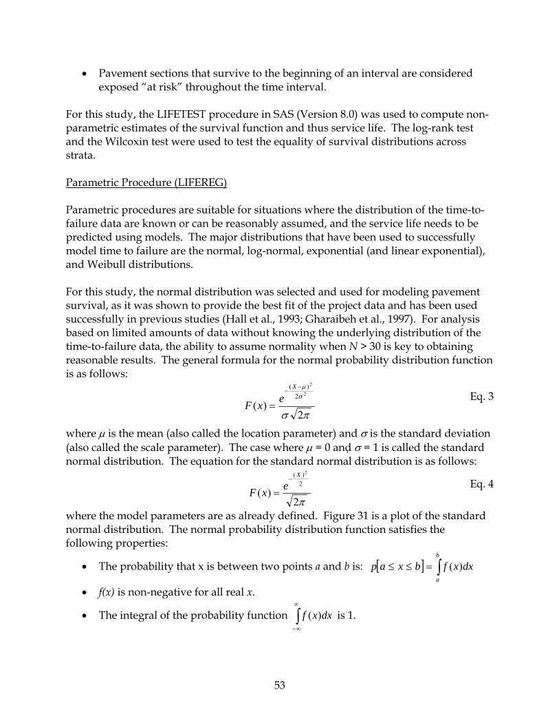
53
• Pavement sections that survive to the beginning of an interval are considered exposed “at risk” throughout the time interval.
For this study, the LIFETEST procedure in SAS (Version 8.0) was used to compute non-parametric estimates of the survival function and thus service life. The log-rank test and the Wilcoxin test were used to test the equality of survival distributions across strata. Parametric Procedure (LIFEREG) Parametric procedures are suitable for situations where the distribution of the time-to-failure data are known or can be reasonably assumed, and the service life needs to be predicted using models. The major distributions that have been used to successfully model time to failure are the normal, log-normal, exponential (and linear exponential), and Weibull distributions. For this study, the normal distribution was selected and used for modeling pavement survival, as it was shown to provide the best fit of the project data and has been used successfully in previous studies (Hall et al., 1993; Gharaibeh et al., 1997). For analysis based on limited amounts of data without knowing the underlying distribution of the time-to-failure data, the ability to assume normality when N > 30 is key to obtaining reasonable results. The general formula for the normal probability distribution function is as follows:
Eq. 3
where µ is the mean (also called the location parameter) and σ is the standard deviation (also called the scale parameter). The case where µ = 0 and σ = 1 is called the standard normal distribution. The equation for the standard normal distribution is as follows:
Eq. 4
where the model parameters are as already defined. Figure 31 is a plot of the standard normal distribution. The normal probability distribution function satisfies the following properties:
• The probability that x is between two points a and b is: [ ] ∫=≤≤b
a
dxxfbxap )(
• f(x) is non-negative for all real x.
• The integral of the probability function ∫∞
∞−
dxxf )( is 1.
πσ
σµ
2)(
2
2
2)( −
−
=
X
exF
π2)(
2)( 2X
exF−
=
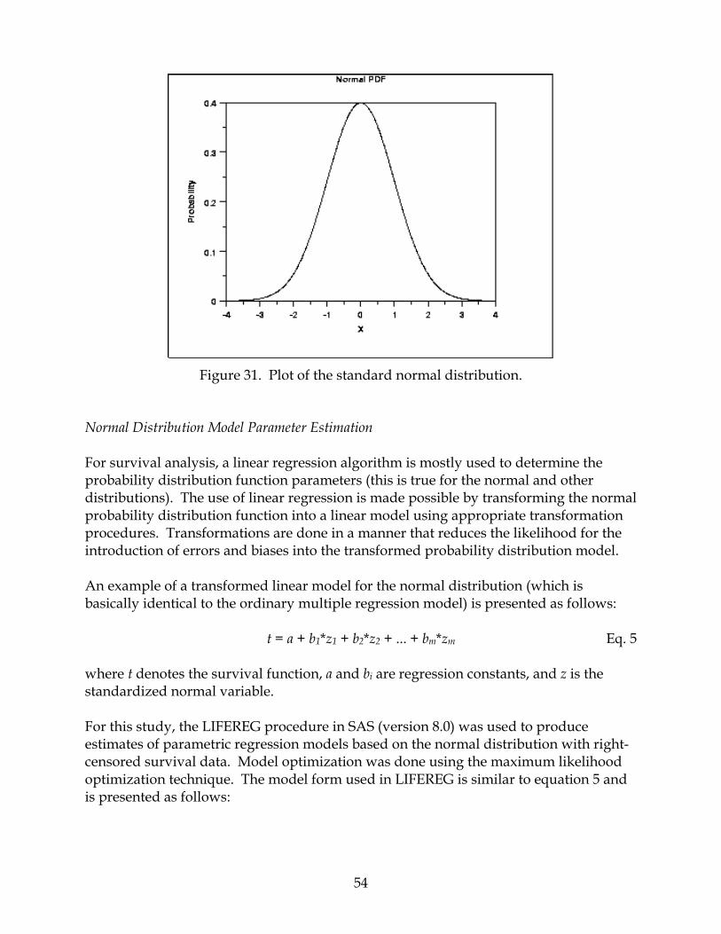
54
Figure 31. Plot of the standard normal distribution. Normal Distribution Model Parameter Estimation For survival analysis, a linear regression algorithm is mostly used to determine the probability distribution function parameters (this is true for the normal and other distributions). The use of linear regression is made possible by transforming the normal probability distribution function into a linear model using appropriate transformation procedures. Transformations are done in a manner that reduces the likelihood for the introduction of errors and biases into the transformed probability distribution model. An example of a transformed linear model for the normal distribution (which is basically identical to the ordinary multiple regression model) is presented as follows: t = a + b1*z1 + b2*z2 + ... + bm*zm Eq. 5 where t denotes the survival function, a and bi are regression constants, and z is the standardized normal variable. For this study, the LIFEREG procedure in SAS (version 8.0) was used to produce estimates of parametric regression models based on the normal distribution with right-censored survival data. Model optimization was done using the maximum likelihood optimization technique. The model form used in LIFEREG is similar to equation 5 and is presented as follows:
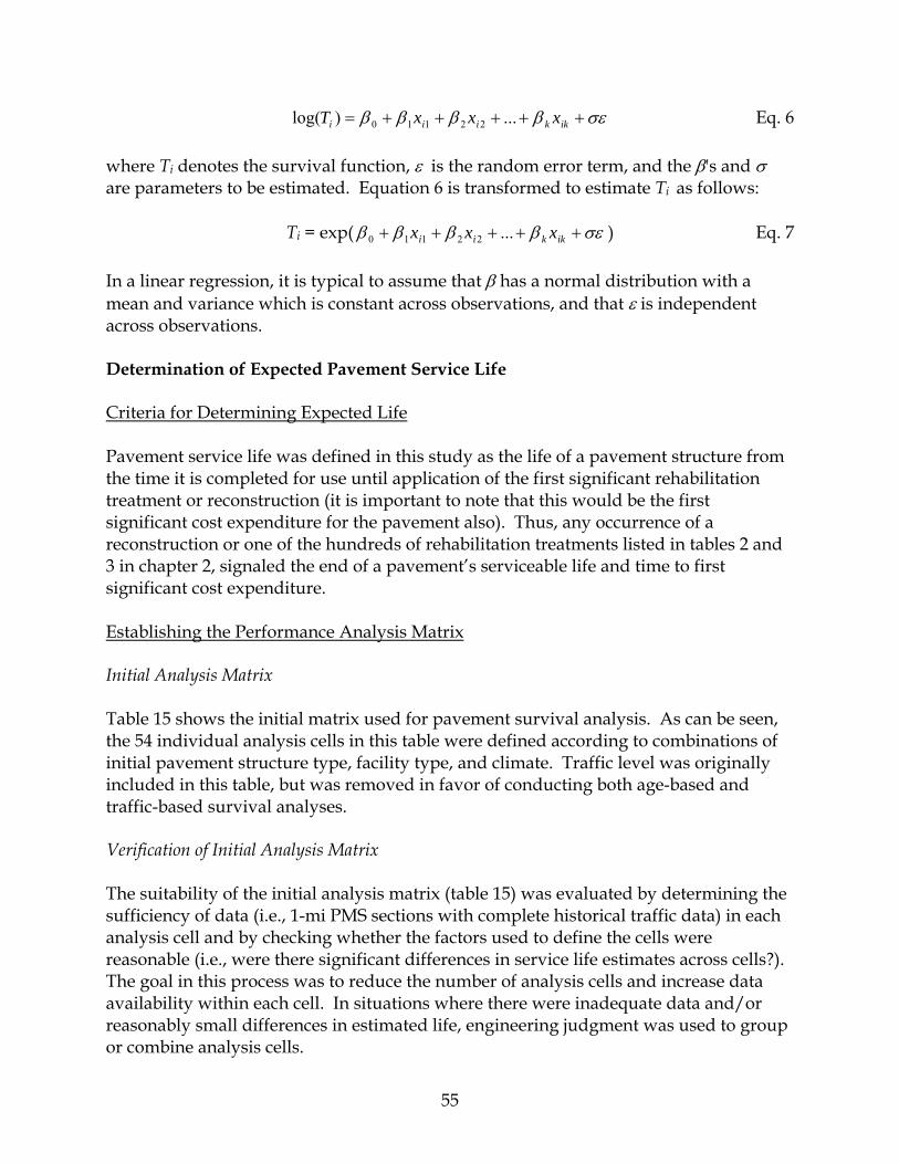
55
σεββββ +++++= ikkiii xxxT ...)log( 22110 Eq. 6 where Ti denotes the survival function, ε is the random error term, and the β's and σ are parameters to be estimated. Equation 6 is transformed to estimate Ti as follows: Ti = exp( σεββββ +++++ ikkii xxx ...22110 ) Eq. 7 In a linear regression, it is typical to assume that β has a normal distribution with a mean and variance which is constant across observations, and that ε is independent across observations. Determination of Expected Pavement Service Life Criteria for Determining Expected Life Pavement service life was defined in this study as the life of a pavement structure from the time it is completed for use until application of the first significant rehabilitation treatment or reconstruction (it is important to note that this would be the first significant cost expenditure for the pavement also). Thus, any occurrence of a reconstruction or one of the hundreds of rehabilitation treatments listed in tables 2 and 3 in chapter 2, signaled the end of a pavement’s serviceable life and time to first significant cost expenditure. Establishing the Performance Analysis Matrix Initial Analysis Matrix Table 15 shows the initial matrix used for pavement survival analysis. As can be seen, the 54 individual analysis cells in this table were defined according to combinations of initial pavement structure type, facility type, and climate. Traffic level was originally included in this table, but was removed in favor of conducting both age-based and traffic-based survival analyses. Verification of Initial Analysis Matrix The suitability of the initial analysis matrix (table 15) was evaluated by determining the sufficiency of data (i.e., 1-mi PMS sections with complete historical traffic data) in each analysis cell and by checking whether the factors used to define the cells were reasonable (i.e., were there significant differences in service life estimates across cells?). The goal in this process was to reduce the number of analysis cells and increase data availability within each cell. In situations where there were inadequate data and/or reasonably small differences in estimated life, engineering judgment was used to group or combine analysis cells.

56
Table 15. Initial pavement survival analysis matrix.
Climate Pavement
Type Facility Type Hot-Dry (RF < 1.5)
Moderate (1.5 < RF < 3.0)
Cool-Wet (RF > 3.0)
Interstates 1 2 3 U.S. Highways 4 5 6 CAC
State Routes 7 8 9 Interstates 10 11 12
U.S. Highways 13 14 15 DSAC State Routes 16 17 18 Interstates 19 20 21
U.S. Highways 22 23 24 FDAC State Routes 25 26 27 Interstates 28 29 30
U.S. Highways 31 32 33 JPC State Routes 34 35 36 Interstates 37 38 39
U.S. Highways 40 41 42 JPCD State Routes 43 44 45 Interstates 46 47 48
U.S. Highways 49 50 51 CRC State Routes 52 53 54
Table 16 summarizes the estimated service life results (in terms of age) of the survival analyses performed for each analysis cell shown in table 15. The results are given in terms of the lives associated with 75%, 50%, and 25% survival probability. Both non-parametric (LIFETEST) and parametric (LIFEREG) results are provided, along with the number of 1-mi sections that comprised each analysis cell. As seen in table 16, 24 of the initial 54 analysis cells had no data (N=0) available for analysis. Furthermore, 16 of the remaining 30 cells had results based on less than 30 data points (N<30), which is the minimum number recommended for analysis. It should also be noted that for some analysis cells, the service lives associated with 75%, 50%, and/or 25% survival probability could not be estimated because the survival rates remained too high for reasonable projection. In these instances, the term “NA” was given to indicate that an estimate was not available. Revised Analysis Matrix Based on the results of the initial survival analysis, the analysis matrix was carefully revised to the one given in table 17. The initial 54 analysis cells were reduced to 15 cells by eliminating cells with no data and combining others with limited data as follows:
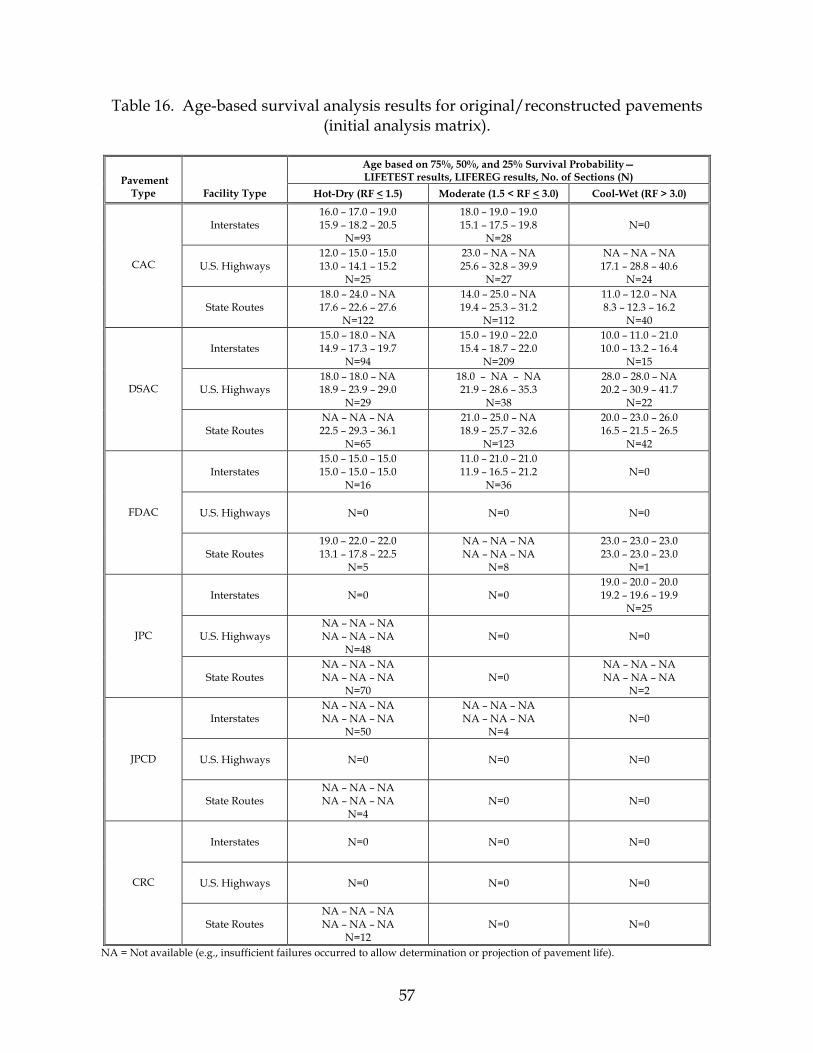
57
Table 16. Age-based survival analysis results for original/reconstructed pavements (initial analysis matrix).
Age based on 75%, 50%, and 25% Survival Probability— LIFETEST results, LIFEREG results, No. of Sections (N) Pavement
Type Facility Type Hot-Dry (RF < 1.5) Moderate (1.5 < RF < 3.0) Cool-Wet (RF > 3.0)
Interstates 16.0 – 17.0 – 19.0 15.9 – 18.2 – 20.5
N=93
18.0 – 19.0 – 19.0 15.1 – 17.5 – 19.8
N=28 N=0
U.S. Highways 12.0 – 15.0 – 15.0 13.0 – 14.1 – 15.2
N=25
23.0 – NA – NA 25.6 – 32.8 – 39.9
N=27
NA – NA – NA 17.1 – 28.8 – 40.6
N=24 CAC
State Routes 18.0 – 24.0 – NA 17.6 – 22.6 – 27.6
N=122
14.0 – 25.0 – NA 19.4 – 25.3 – 31.2
N=112
11.0 – 12.0 – NA 8.3 – 12.3 – 16.2
N=40
Interstates 15.0 – 18.0 – NA 14.9 – 17.3 – 19.7
N=94
15.0 – 19.0 – 22.0 15.4 – 18.7 – 22.0
N=209
10.0 – 11.0 – 21.0 10.0 – 13.2 – 16.4
N=15
U.S. Highways 18.0 – 18.0 – NA 18.9 – 23.9 – 29.0
N=29
18.0 – NA – NA 21.9 – 28.6 – 35.3
N=38
28.0 – 28.0 – NA 20.2 – 30.9 – 41.7
N=22 DSAC
State Routes NA – NA – NA 22.5 – 29.3 – 36.1
N=65
21.0 – 25.0 – NA 18.9 – 25.7 – 32.6
N=123
20.0 – 23.0 – 26.0 16.5 – 21.5 – 26.5
N=42
Interstates 15.0 – 15.0 – 15.0 15.0 – 15.0 – 15.0
N=16
11.0 – 21.0 – 21.0 11.9 – 16.5 – 21.2
N=36
N=0
U.S. Highways
N=0
N=0
N=0
FDAC
State Routes 19.0 – 22.0 – 22.0 13.1 – 17.8 – 22.5
N=5
NA – NA – NA NA – NA – NA
N=8
23.0 – 23.0 – 23.0 23.0 – 23.0 – 23.0
N=1
Interstates
N=0
N=0 19.0 – 20.0 – 20.0 19.2 – 19.6 – 19.9
N=25
U.S. Highways NA – NA – NA NA – NA – NA
N=48
N=0
N=0 JPC
State Routes NA – NA – NA NA – NA – NA
N=70
N=0
NA – NA – NA NA – NA – NA
N=2
Interstates NA – NA – NA NA – NA – NA
N=50
NA – NA – NA NA – NA – NA
N=4
N=0
U.S. Highways
N=0
N=0
N=0 JPCD
State Routes NA – NA – NA NA – NA – NA
N=4
N=0
N=0
Interstates
N=0
N=0
N=0
U.S. Highways
N=0
N=0
N=0 CRC
State Routes NA – NA – NA NA – NA – NA
N=12
N=0
N=0
NA = Not available (e.g., insufficient failures occurred to allow determination or projection of pavement life).

58
Table 17. Revised pavement survival analysis matrix.
Climate Pavement
Type Facility Type Hot-Dry (RF < 1.5)
Moderate (1.5 < RF < 3.0)
Cool-Wet (RF > 3.0)
Interstates 1 2 CAC Non-Interstates
(U.S. Highways & State Routes) 3 4 5
Interstates 6 7 8 DSAC
& FDAC Non-Interstates (U.S. Highways & State Routes) 9 10 11
Interstates JPC Non-Interstates
(U.S. Highways & State Routes) 12 13
Interstates JPCD Non-Interstates
(U.S. Highways & State Routes) 14
Interstates CRC Non-Interstates
(U.S. Highways & State Routes) 15
• For all pavement types, U.S. Highways and State Routes were grouped together under the “Non-Interstates” label.
• For PCC pavements, Interstates and Non-Interstates were grouped together. • FDAC pavements were grouped by climate with DSAC pavements. These two
pavement types have similar structures and surface types, and their survival characteristics are similar.
• The four JPCD pavements in the moderate climate were grouped with JPCD pavements in the hot-dry climate. The regional factor (RF) of 1.7 for these four pavements barely fell outside the 1.5 limit for the hot-dry climate.
Service Life Estimates for Newly Constructed and Reconstructed Pavements Using both non-parametric (LIFETEST) and parametric (LIFEREG) survival analysis procedures, service life estimates were developed for original pavements comprising the 15 revised analysis cells given in table 17. Figures A-1 through A-15 in appendix A show the non-parametric survival curves developed for each analysis cell. These curves show the percentages of section survival as a function of (a) age and (b) cumulative truck traffic. Some of the plots include censored data points, which as indicated previously represent the ages (or cumulative truck applications) of pavement sections that at the time of analysis (2003) had not failed.

59
Tables 18 and 19 summarize the age-based and truck traffic-based initial pavement service lives associated with 75%, 50%, and 25% survival probability. Both LIFETEST and LIFEREG results are listed, along with the number of sections that were included in the analysis. As seen in these tables, limited data (less than 30 sections) existed for the following analysis cells:
• CAC Interstate pavements in moderate climate. • DSAC/FDAC Interstate pavements in cool-wet climate. • JPC pavements in cool-wet climate. • CRC pavements in hot-dry climate.
Once again, for cells where reasonable service life projections could not be made due to high survival rates, an “NA” designation was given. With a couple possible exceptions, the survival analysis results given in tables 18 and 19 appear to be reasonable. The item that needs to be kept in mind is that pavements located on Interstates carry far more truck traffic on average than those off Interstate. Of course, these pavements are designed to carry heavier truck traffic and thus have more substantial structural designs. The median (50% survival probability) ages for the Interstate asphalt pavements are fairly typical for pavements located in the southwestern U.S. Moreover, given the much lower traffic levels of the Non-Interstate routes, the longer median ages for the asphalt pavements was largely expected. With regard to the concrete designs, the 20-year median life for JPC (non-doweled) in the cool-wet climate was derived using sections mostly located on I-17. These sections were built in the mid 1970s and were diamond ground and overlaid (1-in asphalt rubber friction course [FR]) in 1994. Although similar JPC sections on I-40 built in the late 1960s were not included in the analysis because of incomplete traffic data, a review of the database indicated that many of those sections typically survived between 18 and 22 years. Figures 32 and 33 are histograms showing side-by-side comparisons of the median service lives of asphalt and concrete pavements, measured in terms of pavement age and cumulative truck applications. These figures show the significance of design/traffic on the age of a pavement at time of first rehabilitation. For instance, while CAC Non-Interstate pavements lasted longer in terms of time than their Interstate counterparts, they also experienced substantially less truck traffic.
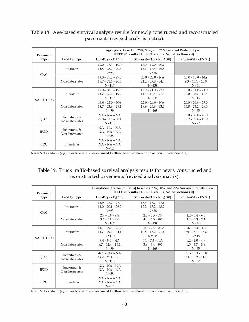
60
Table 18. Age-based survival analysis results for newly constructed and reconstructed pavements (revised analysis matrix).
Age (years) based on 75%, 50%, and 25% Survival Probability—
LIFETEST results, LIFEREG results, No. of Sections (N) Pavement Type Facility Type Hot-Dry (RF < 1.5) Moderate (1.5 < RF < 3.0) Cool-Wet (RF > 3.0)
Interstates 16.0 – 17.0 – 19.0 15.8 – 18.2 – 20.5
N=93
18.0 – 19.0 – 19.0 15.1 – 17.5 – 19.8
N=28
CAC
Non-Interstates 18.0 – 25.0 – 27.0 16.7 – 21.6 – 26.5
N=147
20.0 – 25.0 – NA 21.2 – 27.8 – 34.4
N=139
11.0 – 13.0 – NA 9.3 – 15.1 – 20.8
N=64
Interstates 15.0 – 18.0 – 19.0 14.7 – 16.9 – 19.2
N=110
15.0 – 21.0 – 22.0 14.8 – 18.4 – 21.9
N=245
10.0 – 11.0 – 21.0 10.0 – 13.2 – 16.4
N=15 DSAC & FDAC
Non-Interstates 18.0 – 22.0 – NA 18.7 – 23.9 – 29.1
N=99
22.0 – 26.0 – NA 19.9 – 26.8 – 33.7
N=169
20.0 – 26.0 – 27.0 16.8 – 23.2 – 29.5
N=65
JPC Interstates & Non-Interstates
NA – NA – NA 25.0 – 31.6 – 38.1
N=118
19.0 – 20.0 – 20.0 19.2 – 19.6 – 19.9
N=27
JPCD Interstates & Non-Interstates
NA – NA – NA NA – NA – NA
N=58
CRC Interstates NA – NA – NA NA – NA – NA
N=12
NA = Not available (e.g., insufficient failures occurred to allow determination or projection of pavement life).
Table 19. Truck traffic-based survival analysis results for newly constructed and reconstructed pavements (revised analysis matrix).
Cumulative Trucks (millions) based on 75%, 50%, and 25% Survival Probability—
LIFETEST results, LIFEREG results, No. of Sections (N) Pavement Type Facility Type Hot-Dry (RF < 1.5) Moderate (1.5 < RF < 3.0) Cool-Wet (RF > 3.0)
Interstates 13.9 – 17.2 – 27.4 14.0 – 20.1 – 26.2
N=93
16.6 – 16.7 – 17.6 12.2 – 15.2 – 18.2
N=28
CAC
Non-Interstates 2.7 – 6.0 – 9.8 3.6 – 5.8 – 8.0
N=147
2.8 – 5.3 – 7.5 4.0 – 6.5 – 9.0
N=139
4.2 – 5.4 – 6.5 3.2 – 5.3 – 7.4
N=64
Interstates 14.1 – 19.5 – 26.9 14.7 – 19.4 – 24.1
N=110
8.2 – 17.5 – 20.7 10.8 – 16.2 – 21.6
N=245
10.6 – 17.0 – 18.3 9.5 – 13.1 – 16.8
N=15 DSAC & FDAC
Non-Interstates 7.4 – 9.5 – NA
8.7 – 12.4 – 16.1 N=99
4.1 – 7.3 – NA 3.9 – 6.4 – 9.0
N=169
1.2 – 2.0 – 4.9 1.5 – 3.7 – 5.9
N=65
JPC Interstates & Non-Interstates
47.9 – NA – NA 49.2 – 67.1 – 85.0
N=118
9.1 – 10.3 – 10.8 9.3 – 10.2 – 11.1
N=27
JPCD Interstates & Non-Interstates
NA – NA – NA NA – NA – NA
N=58
CRC Interstates NA – NA – NA NA – NA – NA
N=12
NA = Not available (e.g., insufficient failures occurred to allow determination or projection of pavement life).

61
Figure 32. Comparison of median service life estimates (LIFEREG) for original asphalt
pavements, based on age and cumulative truck applications. Figure 33. Comparison of median service life estimates (LIFEREG) for original concrete
pavements, based on age and cumulative truck applications.
18.2 17.5
21.6
27.8
15.016.9
18.4
13.2
23.9
26.8
23.2
20.1
15.2
5.8 6.55.3
19.4
16.2
13.1 12.4
6.4
3.7
0.0
5.0
10.0
15.0
20.0
25.0
30.0
35.0
CAC,
Int.,
hot
-dry
CAC,
Int.,
mod
erat
eCA
C, N
on-In
t., h
ot-d
ryCA
C, N
on-In
t., m
oder
ate
CAC,
Non
-Int.,
coo
l-wet
DSAC
/FDA
C, In
t., h
ot-d
ryDS
AC/F
DAC,
Int.,
mod
erat
eDS
AC/F
DAC,
Int.,
coo
l-wet
DSAC
/FDA
C, N
on-In
t., h
ot-d
ry
DSAC
/FDA
C, N
on-In
t., m
oder
ate
DSAC
/FDA
C, N
on-In
t., c
ool-w
et
Age
(yrs
), N
o. o
f Tru
cks
(mill
ions
)Time to failure (age in years) Time to failure (no. of trucks applied, millions)
31.6
19.6
67.1
10.2
0.0
10.0
20.0
30.0
40.0
50.0
60.0
70.0
80.0
JPC,
Int.
& No
n-In
t., h
ot-d
ry
JPC,
Int.
& No
n-In
t., c
ool-w
et
JPCD
, Int
. & N
on-In
t., h
ot-d
ry
CRC,
Int.
& No
n-In
t., h
ot-d
ry
Age
(yrs
), N
o. o
f Tru
cks
(mill
ions
)
Time to failure (age in years) Time to failure (no. of trucks applied, millions)
NA NA

62
The same was true for DSAC/FDAC pavements. Also, it can be seen that, while CAC and DSAC/FDAC pavements had fairly similar median ages for a given facility type, the truck levels were typically higher for the DSAC/FDAC pavements. These data tend to show that even though higher type pavements are designed for heavier truck traffic over the same design period, they still do not show the same life until rehabilitation. One possible reason is that the AASHTO structural design may not be considering all aspects of materials, and thus while a pavement may be thicker, the materials properties may not be sufficient to carry the heavier truck traffic. Much more study is needed to clarify the reasons for this finding in survival ages between Interstates and Non-Interstates for asphalt pavements. Figure 33 shows that JPC has survived much longer in hot-dry climate than in a cool-wet climate (32 versus 20 years), even when subjected to far heavier truck traffic in the hot-dry climate (67 versus 10 million trucks). This difference may be explained through the common occurrence of joint faulting in non-doweled JPC, which throughout the U.S. is much greater in cold and wet climates (due to greater joint opening and loss of load transfer efficiency). The survival of JPCD and CRC pavements could not be calculated due to fact that all of the sections are still in service. The ranges in age and cumulative truck traffic for JPCD pavements are 2 to 19 years and 4 to 71 million trucks, whereas the ranges for CRC pavements are 16 years and 6 to 6.5 million trucks. Actual median lives, in terms of age and cumulative truck applications, will be well in excess of these values, since all of the sections are still in service. Figures 34 and 35 provide comparisons of the median initial pavement service life estimates obtained using non-parametric (LIFETEST) and parametric (LIFEREG) procedures. The comparisons show a good correlation between the two sets of estimates (R2 equal to 83 percent in both cases). As such, the predicted lives from parametric procedures (based on the normal distribution) for this data set seems reasonable. Performance Estimates for Rehabilitation Treatments Because of the vast numbers of specific rehabilitation treatments applied over the years to Arizona highways, the analysis of rehabilitation treatment performance life was focused solely on the structure-defined rehabilitation categories (R1 through R13) and structure/mixture-defined categories (i.e., R1A through R13B) presented in tables 2 and 3 in chapter 2. Approximately 3,500 pavement sections, featuring some 4,570 specific treatments, were utilized in the analysis. As with the evaluation of initial pavement service life, only those pavement sections with rehabilitation activities that occurred after 1973 were used, because of the availability of traffic data back to that time.

63
Figure 34. Comparison of median age-based initial service life estimates obtained using
non-parametric (LIFETEST) and parametric (LIFEREG) procedures.
Figure 35. Comparison of median truck-based initial service life estimates obtained using non-parametric (LIFETEST) and parametric (LIFEREG) procedures.
y = 1.1178x - 1.9497R2 = 0.8321
N=12
0
5
10
15
20
25
30
35
0.0 5.0 10.0 15.0 20.0 25.0 30.0 35.0
LIFEREG median service life estimate, years
LIFE
TES
T m
edia
n se
rvic
e lif
e es
timat
e, y
ears
y = 1.1178x - 1.9497R2 = 0.8321
N=12
0
5
10
15
20
25
30
0.0 5.0 10.0 15.0 20.0 25.0 30.0
LIFEREG median service life estimate, cumulative trucks (million)
LIFE
TES
T m
edia
n se
rvic
e lif
e es
timat
e, c
umul
ativ
e tr
ucks
(mill
ion)

64
Results of the survival analyses of structure-defined rehabilitation treatments are presented in tables 20 and 21. These tables list the age-based and truck traffic-based performance lives, corresponding to 75%, 50%, and 25% survival probabilities. Both non-parametric (LIFETEST) and parametric (LIFEREG) results are shown, along with the number of sections that were included in each analysis. As can be seen, there were a substantial number of rehabilitation treatments of asphalt pavements available for analysis and few treatments of concrete pavement available. The predominant treatments for asphalt pavement were thin conventional overlays (R1), shallow removal and thin overlays (R3), and shallow removal and thick overlays (R4). On Interstate pavements, many deep removal and thick overlay treatments (R6) were applied. The predominant treatments for concrete pavement were thin conventional overlays (R1) and diamond grinding (R7). As with the service lives of original asphalt pavements, the lives of rehabilitation treatments applied to asphalt pavements were generally longer for Non-Interstate highways than for Interstate highways. The median age for treatments on U.S. and State routes ranged from 14 to 26 years, compared to a range of 13 to 16 years for treatments on Interstate routes. Tables 20 and 21 also show that the variation in lives (i.e., difference in lives associated with 75% and 25% survival probability) within cells often exceeded the variations observed for original structures. It is believed that the higher variations are partly the result of not separating out (a) the pavement type (e.g., CAC, DSAC, FDAC) on which the rehabilitation was done and (b) the mixture type. Figures A-16 through A-98 in appendix A show the non-parametric survival curves developed for each structure/mixture-defined rehabilitation category for various combinations of facility type and climate. These curves show the percentages of rehabilitated section survival as a function of (a) age and (b) cumulative truck traffic. The rehabilitation categories include the following asphalt mixture types:
• Category A—Conventional asphalt mixes. • Category B—Asphalt rubber mixes. • Category C—SuperPave asphalt mixes. • Category D—Recycled asphalt mixes.
Tables 22 and 23 summarize the performance lives of the structure/mixture-defined rehabilitation categories, derived using both non-parametric (LIFETEST) and parametric (LIFEREG) survival procedures. These tables show that there were a substantial number of rehabilitation treatments utilizing conventional asphalt, asphalt rubber, and recycled asphalt mixes, but much fewer using SuperPave mixes. This was expected since only about 30 SuperPave projects covering the years 1997 through 2001 were included in the database.

65
Table 20. Age-based survival results for structure-defined rehabilitation categories. Age (years) based on 75%, 50%, and 25% Survival Probability—
LIFETEST results, LIFEREG results, No. of Sections (N) Pavement Type
Facility Type Rehab
Category Hot-Dry (RF < 1.5) Moderate (1.5 < RF < 3.0) Cool-Wet (RF > 3.0)
R1 9.0 – 11.0 – 17.0 9.2 – 13.1 – 17.0
N=150
11.0 – 15.0 – 17.0 10.9 – 14.3 – 17.7
N=187
11.0 – NA – NA 14.0 – 20.7 – 27.3
N=22
R2 11.0 – 16.0 – 20.0 10.9 – 14.6 – 18.3
N=11
10.0 – 12.0 – 18.0 11.1 – 15.1 – 19.2
N=78
1.0 – 3.0 – NA 4.6 – 16.1 – 27.7
N=50
R3 10.0 – 13.0 – NA 10.7 – 14.0 – 17.3
N=293
10.0 – 13.0 – NA 10.2 – 13.4 – 16.6
N=261
11.0 – 11.0 – 11.0 10.5 – 12.3 – 14.1
N=13
R4 14.0 – 17.0 – 17.0 11.7 – 15.4 – 19.1
N=430
11.0 – 15.0 – 18.0 11.6 – 14.9 – 18.1
N=470 N=0
R5 N=0 NA – NA – NA NA – NA – NA
N=8 N=0
Interstates
R6 14.0 – 14.0 – 21.0 12.5 – 15.4 – 18.3
N=189
10.0 – 17.0 – 17.0 11.4 – 14.2 – 16.9
N=173
NA – NA – NA NA – NA – NA
N=6
R1 16.0 – NA – NA 17.7 – 24.3 – 30.9
N=280
17.0 – 23.0 – NA 16.0 – 23.6 – 31.2
N=1,030
13.0 – 23.0 – NA 11.9 – 19.9 – 28.0
N=328
R2 17.0 – NA – NA 17.9 – 26.4 – 34.9
N=20
15.0 – 23.0 – NA 18.8 – 24.9 – 33.0
N=63
NA – NA – NA NA – NA – NA
N=7
R3 10.0 – NA – NA 11.7 – 17.2 – 22.8
N=121
15.0 – 17.0 – 19.0 13.6 – 17.6 – 21.5
N=125
NA – NA – NA 14.1 – 18.5 – 22.9
N=29
R4 14.0 – 15.0 – 16.0 13.9 – 16.2 – 18.5
N=54
NA – NA – NA 13.0 – 14.0 – 15.1
N=84
NA – NA – NA NA – NA – NA
N=21
CAC, DSAC, & FDAC
Non-Interstates
R6 18.0 – NA – NA 19.0 – 21.3 – 23.7
N=4
3.0 – 19.0 – NA 9.1 – 16.7 – 24.3
N=12
9.0 – 9.0 – NA 9.0 – 9.9 – 10.8
N=3
R1 N=0 2.0 – 10.0 – NA 5.4 – 13.5 – 21.7
N=8
10.0 – 10.0 – 14.0 9.7 – 11.4 – 13.1
N=32
R2 N=0 NA – NA – NA NA – NA– NA
N=6
NA – NA – NA NA – NA – NA
N=9
R3 N=0 NA – NA – NA NA – NA – NA
N=1
NA – NA – NA NA – NA – NA
N=22
R5 N=0 11.0 – 11.0 – 11.0 11.0 – 11.0 – 11.0
N=1
11.0 – 11.0 – 11.0 11.0 – 11.0 – 11.0
N=6
R7 14.0 – 15.0 – 16.0 13.3 – 15.4 – 17.5
N=22
10.0 – 12.0 – 12.0 10.6 – 11.4 – 12.3
N=29 N=0
R10 N=0 N=0 NA – NA – NA NA – NA – NA
N=25
R12 N=0 N=0 9.0 – NA – NA
10.8 – 15.7 – 20.6 N=14
JPC Interstates & Non-Interstates
R13 N=0 N=0 NA – NA – NA NA – NA – NA
N=9
JPCD & CRC Interstates & Non-Interstates R7
NA – NA – NA NA – NA – NA
N=4 N=0 N=0
NA = Not available (e.g., insufficient failures occurred to allow determination or projection of treatment life).

66
Table 21. Truck traffic-based survival results for structure-defined rehabilitation categories.
Cumulative Trucks (millions) based on 75%, 50%, and 25% Survival Probability—LIFETEST results, LIFEREG results, No. of Sections (N) Pavement
Type
Facility Type Rehab
Category Hot-Dry (RF < 1.5) Moderate (1.5 < RF < 3.0) Cool-Wet (RF > 3.0)
R1 5.0 – 6.0 – 13.6 3.9 – 11.0 – 18.0
N=150
14.0 – 19.5 – 22.2 12.9 – 18.7 – 24.4
N=187
4.7 – NA – NA 13.5 – 32.6 – 51.8
N=22
R2 7.9 – 16.1 – 16.1 7.7 – 15.7 – 23.7
N=11
13.8 – 17.4 – 30.9 13.7 – 20.7 – 27.7
N=78
0.9 – 2.6 – NA 5.5 – 24.6 – 43.7
N=50
R3 16.1 – 20.1 – 37.7 15.6 – 23.2 – 30.7
N=293
11.3 – NA – NA 18.0 – 28.5 – 38.9
N=261
6.8 – 6.8 – 7.2 7.0 – 8.5 – 10.0
N=13
R4 11.7 – 25.9 – NA 16.9 – 27.9 – 38.8
N=430
15.9 – 26.6 – NA 17.6 – 26.0 – 34.4
N=470 N=0
R5 N=0 NA – NA – NA NA – NA – NA
N=8 N=0
Interstates
R6 32.5 – 39.9 – 39.9 25.3 – 36.3 – 47.2
N=189
30.9 – 30.9 – 30.9 22.4 – 29.1 – 35.8
N=173
NA – NA – NA 9.0 – 15.7 – 22.4
N=6
R1 3.0 – 6.3 – 18.5 4.5 – 6.8 – 9.1
N=280
1.5 – 3.5 – 7.4 2.0 – 3.5 – 5.1
N=1,030
0.7 – 2.4 – 6.8 1.4 – 3.0 – 4.5
N=328
R2 5.4 – NA – NA 8.4 – 17.1 – 25.9
N=20
2.1 – 5.4 – NA 2.7 – 4.9 – 7.2
N=63
3.4 – NA – NA 8.8 – 13.9 – 19.0
N=7
R3 3.7 – NA – NA 6.8 – 13.4 – 20.0
N=121
1.8 – 7.3 – 8.1 2.9 – 4.7 – 6.6
N=125
NA – NA – NA 7.9 – 13.1 – 18.4
N=29
R4 2.0 – 3.6 – 11.1 3.5 – 5.6 – 7.6
N=54
NA – NA – NA 10.3 – 13.8 – 17.3
N=84
NA – NA – NA NA – NA – NA
N=21
CAC, DSAC, & FDAC
Non-Interstates
R6 11.2 – 11.2 – 11.2 NA – NA – NA
N=4
0.3 – 0.8 – 2.4 0.6 – 1.2 – 1.9
N=12
1.2 – 1.2 – NA 1.2 – 1.3 – 1.5
N=3
R1 N=0
0.2 – 11.6 – 13.8 3.2 – 8.0 – 12.7
N=8
10.0 – 13.8 – 20.5 11.3 – 14.7 – 18.0
N=32
R2 N=0 NA – NA – NA NA – NA– NA
N=6
NA – NA – NA NA – NA – NA
N=9
R3 N=0 NA – NA – NA NA – NA – NA
N=1
NA – NA – NA NA – NA – NA
N=22
R5 N=0 18.3 – 18.3 – 18.3 18.3 – 18.3 – 18.3
N=1
16.8 – 17.6 – 18.3 17.0 – 17.5 – 18.1
N=6
R7 47.7 – 56.0 – 64.8 48.0 – 54.6 – 61.2
N=22
15.12 – 45.1 – 50.8 26.2 – 37.1 – 47.9
N=29 N=0
R10 N=0 N=0 NA – NA – NA NA – NA – NA
N=25
R12 N=0 N=0 14.1 – NA – NA 17.1 – 26.1 – 35.0
N=14
JPC Interstates & Non-Interstates
R13 N=0 N=0 NA – NA – NA NA – NA – NA
N=9
JPCD & CRC Interstates & Non-Interstates R7
NA – NA – NA NA – NA – NA
N=4 N=0 N=0
NA = Not available (e.g., insufficient failures occurred to allow determination or projection of treatment life).

67
Table 22. Age-based survival results for structure/mixture-defined rehabilitation categories. Age (years) based on 75%, 50%, and 25% Survival Probability—
LIFETEST results, LIFEREG results, No. of Sections (N) Pavement Type
Facility Type Rehab
Category Hot-Dry (RF < 1.5) Moderate (1.5 < RF < 3.0) Cool-Wet (RF > 3.0)
R1A 9.0 – 11.0 – 17.0 9.2 – 13.1 – 17.0
N=150
10.0 – 15.0 – 17.0 10.9 – 14.3 – 17.8
N=180
NA – NA – NA NA – NA – NA
N=12
R1B N=0 14.0 – 14.0 – 14.0 14.0 – 14.0 – 14.0
N=7
11.0 – 11.0 – 11.0 11.0 – 11.0 – 11.0
N=10
R2A 11.0 – 16.0 – 20.0 10.9 – 14.6 – 18.3
N=11
10.0 – 12.0 – 18.0 11.1 – 15.1 – 19.2
N=78
1.0 – 3.0 – NA 4.6 – 16.1 – 27.7
N=50
R3A 9.0 – 11.0 – 13.0 9.2 – 10.9 – 12.6
N=77
8.0 – 11.0 – NA 9.0 – 12.6 – 16.3
N=112 N=0
R3B NA – NA – NA 12.4 – NA – NA
N=183
11.0 – NA – NA 10.6 – NA – NA
N=122
NA – NA – NA NA – NA – NA
N=6
R3C N=0 NA – NA – NA NA – NA – NA
N=6 N=0
R3D 13.0 – NA – NA 14.9 – 21.9 – NA
N=33
11.0 – 13.0 – NA 11.8 – 14.3 – 16.7
N=21
11.0 – 11.0 – 11.0 10.2 – 12.1 – 14.1
N=7
R4A NA – NA – NA NA – NA – NA
N=56
NA – NA – NA 16.6 – NA – NA
N=148 N=0
R4B NA – NA – NA 12.4 – NA – NA
N=146
NA – NA – NA 11.0 – NA – NA
N=94 N=0
R4C N=0 NA – NA – NA NA – NA – NA
N=32 N=0
R4D 14.0 – 16.0 – 17.0 11.7 – 15.1 – 18.5
N=228
10.0 – 14.0 – 18.0 11.5 – 13.9 – 16.4
N=196 N=0
R5A N=0 NA – NA – NA NA – NA – NA
N=1 N=0
R6A NA – NA – NA NA – NA – NA
N=21
10.0 – 10.0 – 17.0 9.9 – 11.4 – 12.8
N=14 N=0
R6B NA – NA – NA NA – NA – NA
N=79
NA – NA – NA NA – NA – NA
N=97
NA – NA – NA 9.8 – NA– NA
N=6
R6C NA – NA – NA NA – NA – NA
N=41
NA – NA – NA NA – NA – NA
N=38 N=0
CAC, DSAC, & FDAC Interstates
R6D 8.0 – 14.0 – 14.0 10.4 – 13.5 – 16.7
N=48
NA – NA – NA NA – NA – NA
N=24 N=0
NA = Not available (e.g., insufficient failures occurred to allow determination or projection of treatment life).
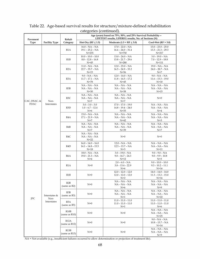
68
Table 22. Age-based survival results for structure/mixture-defined rehabilitation categories (continued).
Age (years) based on 75%, 50%, and 25% Survival Probability— LIFETEST results, LIFEREG results, No. of Sections (N) Pavement
Type
Facility Type Rehab
Category Hot-Dry (RF < 1.5) Moderate (1.5 < RF < 3.0) Cool-Wet (RF > 3.0)
R1A 16.0 – NA – NA 19.1 – 25.2 – NA
N=235
17.0 – 22.0 – NA 16.6 – 24.0 – 31.4
N=750
13.0 – 23.0 – 25.0 13.3 – 21.3 – 29.3
N=217
R1B 10.0 – 10.0 – 10.0 8.8 – 12.8 – 16.8
N=45
13.0 – 24.0 – NA 13.8 – 21.7 – 29.6
N=280
3.0 – 19.0 – NA 7.0 – 12.9 – 18.8
N=111
R2A 11.0 – NA – NA 22.7 – 35.7 – NA
N=15
12.0 – 23.0 – NA 16.5 – 24.9 – 33.2
N=56
19.0 – NA – NA 24.0 – 28.7 – NA
N=7
R3A 9.0 – NA – NA
11.7 – 17.1 – NA N=78
12.0 – 14.0 – NA 11.8 – 14.5 – 17.2
N=45
9.0 – NA – NA 11.6 – 15.3 – 19.0
N=10
R3B NA – NA – NA NA – NA – NA
N=30
NA – NA – NA NA – NA – NA
N=38
NA – NA – NA NA – NA – NA
N=15
R3C NA – NA – NA NA – NA – NA
N=7
NA – NA – NA NA – NA – NA
N=7 N=0
R3D 3.0 – 3.0 – 3.0
1.0 – 6.7 – 12.4 N=6
17.0 – 17.0 – 19.0 14.8 – 19.4 – 24.0
N=35
NA – NA – NA NA – NA – NA
N=4
R4A 15.0 – NA – NA 17.1 – 21.9 – NA
N=7
NA – NA – NA NA – NA – NA
N=42
NA – NA – NA NA – NA – NA
N=3
R4B NA – NA – NA NA – NA – NA
N=7
NA – NA – NA NA – NA – NA
N=39
NA – NA – NA NA – NA – NA
N=7
R4C NA – NA – NA NA – NA – NA
N=22 N=0 N=0
R4D 14.0 – 14.0 – 16.0 14.1 – 14.8 – 15.5
N=18
12.0 – NA – NA 12.5 – 13.7 – NA
N=3
NA – NA – NA NA – NA – NA
N=11
CAC, DSAC, & FDAC
Non-Interstates
R6A 18.0 – NA – NA 19.0 – 21.3 – NA
N=4
3.0 – 19.0 – NA 9.0 – 16.7 – 24.3
N=12
9.0 – 9.0 – NA 9.0 – 9.9 – 10.8
N=3
R1A N=0 2.0 – 6.0 – NA
3.8 – 13.4 – 22.9 N=6
9.0 – 10.0 – 10.0 9.3 – 10.2 – 11.1
N=16
R1B N=0 12.0 – 12.0 – 12.0 12.0 – 12.0 – 12.0
N=2
14.0 – 14.0 – 14.0 11.3 – 13.2 – 15.0
N=16
R2B (same as R2) N=0
NA – NA – NA NA – NA – NA
N=6
NA – NA – NA NA – NA – NA
N=9
R3B (same as R3) N=0
NA – NA – NA NA – NA – NA
N=1
NA – NA – NA NA – NA – NA
N=22
R5A (same as R5) N=0
11.0 – 11.0 – 11.0 11.0 – 11.0 – 11.0
N=1
11.0 – 11.0 – 11.0 11.0 – 11.0 – 11.0
N=6
R10B (same as R10) N=0 N=0
NA – NA – NA NA – NA – NA
N=25
R12A (same as R12) N=0 N=0
9.0 – NA – NA 10.8 – 15.7 – NA
N=14
JPC Interstates &
Non-Interstates
R13B (same as R13) N=0 N=0
NA – NA – NA NA – NA – NA
N=9 NA = Not available (e.g., insufficient failures occurred to allow determination or projection of treatment life).
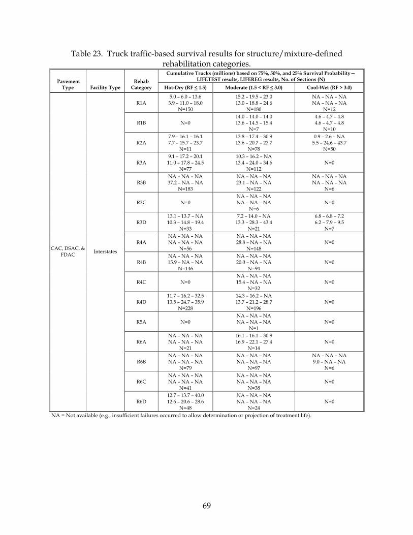
69
Table 23. Truck traffic-based survival results for structure/mixture-defined rehabilitation categories.
Cumulative Trucks (millions) based on 75%, 50%, and 25% Survival Probability— LIFETEST results, LIFEREG results, No. of Sections (N) Pavement
Type
Facility Type Rehab
Category Hot-Dry (RF < 1.5) Moderate (1.5 < RF < 3.0) Cool-Wet (RF > 3.0)
R1A 5.0 – 6.0 – 13.6 3.9 – 11.0 – 18.0
N=150
15.2 – 19.5 – 23.0 13.0 – 18.8 – 24.6
N=180
NA – NA – NA NA – NA – NA
N=12
R1B N=0 14.0 – 14.0 – 14.0 13.6 – 14.5 – 15.4
N=7
4.6 – 4.7 – 4.8 4.6 – 4.7 – 4.8
N=10
R2A 7.9 – 16.1 – 16.1 7.7 – 15.7 – 23.7
N=11
13.8 – 17.4 – 30.9 13.6 – 20.7 – 27.7
N=78
0.9 – 2.6 – NA 5.5 – 24.6 – 43.7
N=50
R3A 9.1 – 17.2 – 20.1 11.0 – 17.8 – 24.5
N=77
10.3 – 16.2 – NA 13.4 – 24.0 – 34.6
N=112 N=0
R3B NA – NA – NA 37.2 – NA – NA
N=183
NA – NA – NA 23.1 – NA – NA
N=122
NA – NA – NA NA – NA – NA
N=6
R3C N=0 NA – NA – NA NA – NA – NA
N=6 N=0
R3D 13.1 – 13.7 – NA 10.3 – 14.8 – 19.4
N=33
7.2 – 14.0 – NA 13.3 – 28.3 – 43.4
N=21
6.8 – 6.8 – 7.2 6.2 – 7.9 – 9.5
N=7
R4A NA – NA – NA NA – NA – NA
N=56
NA – NA – NA 28.8 – NA – NA
N=148 N=0
R4B NA – NA – NA 15.9 – NA – NA
N=146
NA – NA – NA 20.0 – NA – NA
N=94 N=0
R4C N=0 NA – NA – NA 15.4 – NA – NA
N=32 N=0
R4D 11.7 – 16.2 – 32.5 13.5 – 24.7 – 35.9
N=228
14.3 – 16.2 – NA 13.7 – 21.2 – 28.7
N=196 N=0
R5A N=0 NA – NA – NA NA – NA – NA
N=1 N=0
R6A NA – NA – NA NA – NA – NA
N=21
16.1 – 16.1 – 30.9 16.9 – 22.1 – 27.4
N=14 N=0
R6B NA – NA – NA NA – NA – NA
N=79
NA – NA – NA NA – NA – NA
N=97
NA – NA – NA 9.0 – NA – NA
N=6
R6C NA – NA – NA NA – NA – NA
N=41
NA – NA – NA NA – NA – NA
N=38 N=0
CAC, DSAC, & FDAC Interstates
R6D 12.7 – 13.7 – 40.0 12.6 – 20.6 – 28.6
N=48
NA – NA – NA NA – NA – NA
N=24 N=0
NA = Not available (e.g., insufficient failures occurred to allow determination or projection of treatment life).
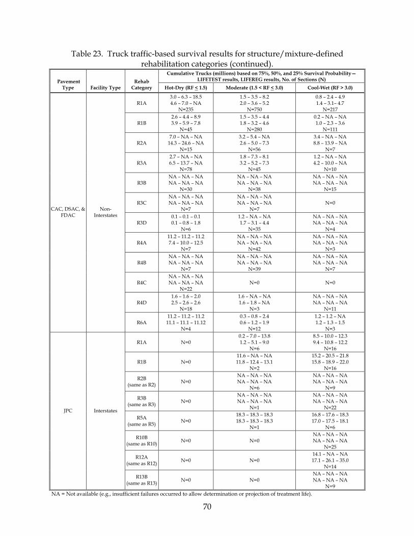
70
Table 23. Truck traffic-based survival results for structure/mixture-defined rehabilitation categories (continued).
Cumulative Trucks (millions) based on 75%, 50%, and 25% Survival Probability— LIFETEST results, LIFEREG results, No. of Sections (N) Pavement
Type
Facility Type Rehab
Category Hot-Dry (RF < 1.5) Moderate (1.5 < RF < 3.0) Cool-Wet (RF > 3.0)
R1A 3.0 – 6.3 – 18.5 4.6 – 7.0 – NA
N=235
1.5 – 3.5 – 8.2 2.0 – 3.6 – 5.2
N=750
0.8 – 2.4 – 4.9 1.4 – 3.1– 4.7
N=217
R1B 2.6 – 4.4 – 8.9 3.9 – 5.9 – 7.8
N=45
1.5 – 3.5 – 4.4 1.8 – 3.2 – 4.6
N=280
0.2 – NA – NA 1.0 – 2.3 – 3.6
N=111
R2A 7.0 – NA – NA
14.3 – 24.6 – NA N=15
3.2 – 5.4 – NA 2.6 – 5.0 – 7.3
N=56
3.4 – NA – NA 8.8 – 13.9 – NA
N=7
R3A 2.7 – NA – NA 6.5 – 13.7 – NA
N=78
1.8 – 7.3 – 8.1 3.2 – 5.2 – 7.3
N=45
1.2 – NA – NA 4.2 – 10.0 – NA
N=10
R3B NA – NA – NA NA – NA – NA
N=30
NA – NA – NA NA – NA – NA
N=38
NA – NA – NA NA – NA – NA
N=15
R3C NA – NA – NA NA – NA – NA
N=7
NA – NA – NA NA – NA – NA
N=7 N=0
R3D 0.1 – 0.1 – 0.1 0.1 – 0.8 – 1.8
N=6
1.2 – NA – NA 1.7 – 3.1 – 4.4
N=35
NA – NA – NA NA – NA – NA
N=4
R4A 11.2 – 11.2 – 11.2 7.4 – 10.0 – 12.5
N=7
NA – NA – NA NA – NA – NA
N=42
NA – NA – NA NA – NA – NA
N=3
R4B NA – NA – NA NA – NA – NA
N=7
NA – NA – NA NA – NA – NA
N=39
NA – NA – NA NA – NA – NA
N=7
R4C NA – NA – NA NA – NA – NA
N=22 N=0 N=0
R4D 1.6 – 1.6 – 2.0 2.5 – 2.6 – 2.6
N=18
1.6 – NA – NA 1.6 – 1.8 – NA
N=3
NA – NA – NA NA – NA – NA
N=11
CAC, DSAC, & FDAC
Non-Interstates
R6A 11.2 – 11.2 – 11.2
11.1 – 11.1 – 11.12 N=4
0.3 – 0.8 – 2.4 0.6 – 1.2 – 1.9
N=12
1.2 – 1.2 – NA 1.2 – 1.3 – 1.5
N=3
R1A N=0 0.2 – 7.0 – 13.8 1.2 – 5.1 – 9.0
N=6
8.5 – 10.0 – 12.3 9.4 – 10.8 – 12.2
N=16
R1B N=0 11.6 – NA – NA 11.8 – 12.4 – 13.1
N=2
15.2 – 20.5 – 21.8 15.8 – 18.9 – 22.0
N=16
R2B (same as R2) N=0
NA – NA – NA NA – NA – NA
N=6
NA – NA – NA NA – NA – NA
N=9
R3B (same as R3) N=0
NA – NA – NA NA – NA – NA
N=1
NA – NA – NA NA – NA – NA
N=22
R5A (same as R5) N=0
18.3 – 18.3 – 18.3 18.3 – 18.3 – 18.3
N=1
16.8 – 17.6 – 18.3 17.0 – 17.5 – 18.1
N=6
R10B (same as R10) N=0 N=0
NA – NA – NA NA – NA – NA
N=25
R12A (same as R12) N=0 N=0
14.1 – NA – NA 17.1 – 26.1 – 35.0
N=14
JPC Interstates
R13B (same as R13) N=0 N=0
NA – NA – NA NA – NA – NA
N=9 NA = Not available (e.g., insufficient failures occurred to allow determination or projection of treatment life).

71
Figures 36 and 37 show the median performance lives (parametric LIFEREG) of conventional asphalt mixes when used with different structure-defined rehabilitation categories (R1 through R6). It can generally be seen that, although the median ages remain similar across the categories—11 to 16 years on Interstates, 15 to 25 years on Non-Interstates—the median truck traffic increases corresponding to thicker rehabilitation treatments. Moreover, although the effect of climate on conventional asphalt mix performance was not as profound as expected, there did seem to be some impact on Non-Interstate routes, with performance being generally better in the hot-dry regions and worse in the cool-wet. Figures 38 through 41 present side-by-side comparisons of the median performance lives (parametric LIFEREG) of asphalt pavement rehabilitation treatments, measured in terms of pavement age and cumulative truck applications. Each figure represents an individual structure category (e.g., R1=thin conventional overlay), and the performance of the four different asphalt mixtures for that category are displayed (where available), corresponding to facility type and climate. A comparison of conventional asphalt mixes with asphalt rubber mixes yielded conflicting performance results. For thin conventional overlays (R1) placed on Non-Interstate asphalt pavements, better performance was experienced with conventional asphalt mix than with asphalt rubber (23 to 25 years versus 13 to 22 years) for fairly similar truck traffic levels. On the other hand, for shallow removal and thin overlays
Figure 36. Performance life of conventional asphalt mix when used in different structure-defined rehabilitations applied to Interstate asphalt pavements.
0
5
10
15
20
25
30
35
40
R1A R2A R3A R4A R5A R6A R1A R2A R3A R4A R5A R6A R1A R2A R3A R4A R5A R6A
Hot-Dry Moderate Cool-Wet
Age
(yea
rs),
No.
of T
ruck
s (m
illio
ns)
Age Cumulative Trucks
1=ACOL (1.5"<thick<4") 2=ACOL (thick>4")3=Mill (depth<4") & ACOL (1.5"<thick<4") 4=Mill (depth<4") & ACOL (thick>4")5=Mill (depth>4") & ACOL (1.5"<thick<4") 6=Mill (depth>4") & ACOL (thick>4")

72
Figure 37. Performance life of conventional asphalt mix when used in different structure-defined rehabilitations applied to Non-Interstate asphalt pavements.
Figure 38. Performance life of thin conventional overlays (R1) on asphalt pavement using different asphalt mixture types.
0
5
10
15
20
25
30
I NI I NI I NI I NI I NI I NI I NI I NI I NI I NI I NI I NI
R1A R1B R1C R1D R1A R1B R1C R1D R1A R1B R1C R1D
Hot-Dry Moderate Cool-Wet
Age
(yea
rs),
No.
of t
ruck
s (m
illio
ns)
Age Cumulative Trucks
A=Conv. asphaltB=Asphalt rubberC=SuperPaveD=Recycled asphalt
0
5
10
15
20
25
30
35
40
R1A R2A R3A R4A R5A R6A R1A R2A R3A R4A R5A R6A R1A R2A R3A R4A R5A R6A
Hot-Dry Moderate Cool-Wet
Age
(yea
rs),
No.
of T
ruck
s (m
illio
ns)
Age Cumulative Trucks
1=ACOL (1.5"<thick<4") 2=ACOL (thick>4")3=Mill (depth<4") & ACOL (1.5"<thick<4") 4=Mill (depth<4") & ACOL (thick>4")5=Mill (depth>4") & ACOL (1.5"<thick<4") 6=Mill (depth>4") & ACOL (thick>4")

73
Figure 39. Performance life of shallow removal and thin overlays (R3) on asphalt pavement using different asphalt mixture types.
Figure 40. Performance life of shallow removal and thick overlays (R4) on asphalt pavement using different asphalt mixture types.
0
5
10
15
20
25
30
35
40
I NI I NI I NI I NI I NI I NI I NI I NI I NI I NI I NI I NI
R3A R3B R3C R3D R3A R3B R3C R3D R3A R3B R3C R3D
Hot-Dry Moderate Cool-Wet
Age
(yea
rs),
No.
of T
ruck
s (m
illio
ns)
Age Cumulative Trucks
Life based on 75% survival probability
A=Conv. asphaltB=Asphalt rubberC=SuperPaveD=Recycled asphalt
0
5
10
15
20
25
30
35
I NI I NI I NI I NI I NI I NI I NI I NI I NI I NI I NI I NI
R4A R4B R4C R4D R4A R4B R4C R4D R4A R4B R4C R4D
Hot-Dry Moderate Cool-Wet
Age
(yea
rs),
No.
of T
ruck
s (m
illio
ns)
Age Cumulative Trucks
Life based on 75% survival probability
A=Conv. asphaltB=Asphalt rubberC=SuperPaveD=Recycled asphalt

74
Figure 41. Performance life of deep removal and thick overlays (R6) on asphalt pavement using different asphalt mixture types.
(R3) placed on Interstate pavements, the asphalt rubber mix yielded better performance than the conventional mix (similar or longer lives for significantly higher levels of truck traffic). With regard to other mix types, similar or better performance was experienced by some treatments (R3 on Interstate and Non-Interstate pavements) using recycled asphalt mixes, as compared to conventional asphalt mixes. A comparison of SuperPave mix performance could not be made, as all sections containing this mix type were relatively young (<6 years) and still in service. Figure 42 shows the median lives of conventional asphalt and asphalt rubber mixes, when applied as part of a thin overlay on JPC pavements. Although based on a limited number of sections, it can be seen that the age survival of the two mixes are similar (10 to 13 years), but that the asphalt rubber treatments received significantly more truck traffic (about 7 million more trucks in each case). Figures 43 and 44 provide comparisons of the median structure/mixture-defined rehabilitation life estimates obtained using non-parametric (LIFETEST) and parametric (LIFEREG) procedures. The comparisons show a fairly good correlation between the two sets of estimates (R2 equal to about 0.63 in both cases). As such, the predicted lives from parametric procedures (based on the normal distribution) for this data set seem reasonable.
0
5
10
15
20
25
I NI I NI I NI I NI I NI I NI I NI I NI I NI I NI I NI I NI
R6A R6B R6C R6D R6A R6B R6C R6D R6A R6B R6C R6D
Hot-Dry Moderate Cool-Wet
Age
(yea
rs),
No.
of T
ruck
s (m
illio
ns)
Age Cumulative Trucks
Life based on 75% survival probability
A=Conv. asphaltB=Asphalt rubberC=SuperPaveD=Recycled asphalt
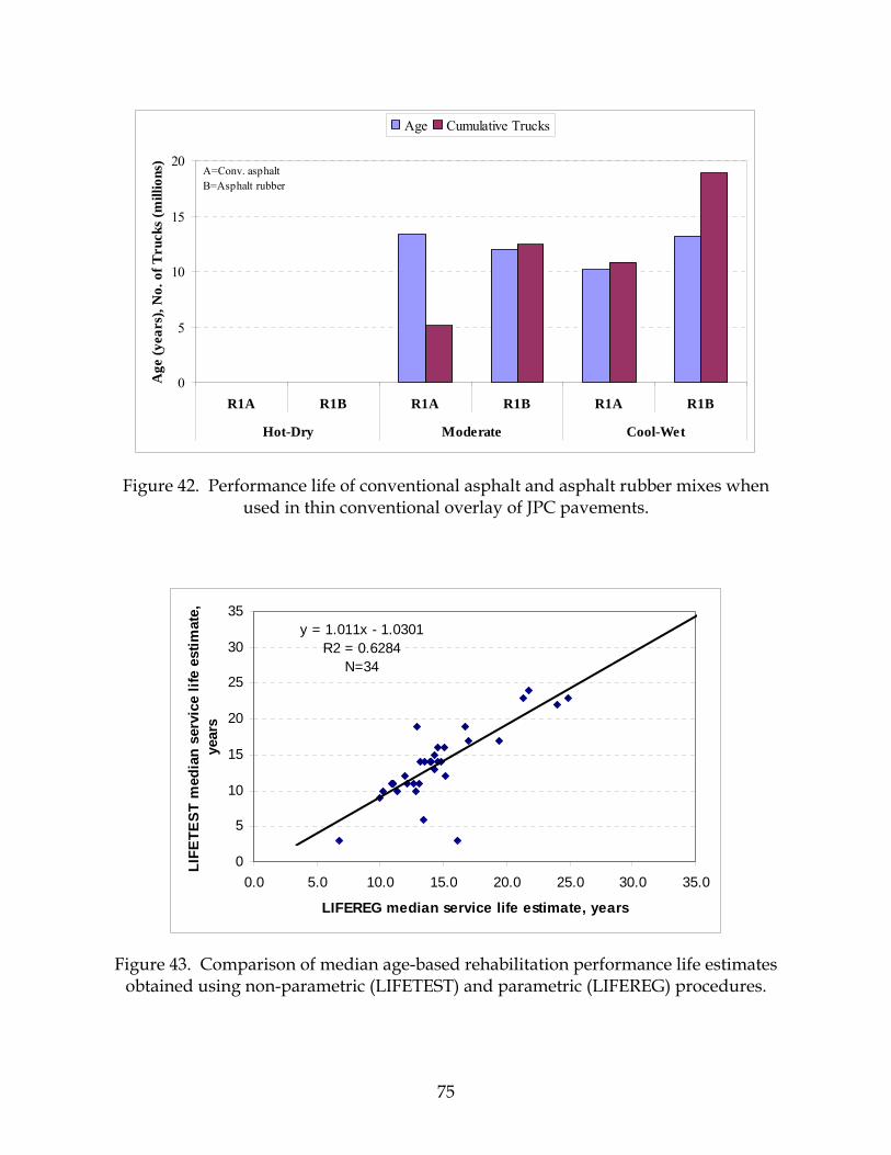
75
Figure 42. Performance life of conventional asphalt and asphalt rubber mixes when used in thin conventional overlay of JPC pavements.
Figure 43. Comparison of median age-based rehabilitation performance life estimates obtained using non-parametric (LIFETEST) and parametric (LIFEREG) procedures.
y = 1.011x - 1.0301R2 = 0.6284
N=34
0
5
10
15
20
25
30
35
0.0 5.0 10.0 15.0 20.0 25.0 30.0 35.0
LIFEREG median service life estimate, years
LIFE
TEST
med
ian
serv
ice
life
estim
ate,
ye
ars
0
5
10
15
20
R1A R1B R1A R1B R1A R1B
Hot-Dry Moderate Cool-Wet
Age
(yea
rs),
No.
of T
ruck
s (m
illio
ns)
Age Cumulative Trucks
A=Conv. asphaltB=Asphalt rubber

76
Figure 44. Comparison of median truck-based rehabilitation performance life estimates
obtained using non-parametric (LIFETEST) and parametric (LIFEREG) procedures. MECHANISTIC-BASED PERFORMANCE ANALYSIS Mechanistic-based analysis was conducted to determine if the estimates of service life were comparable to the results from survival analyses in Arizona over a broad range of pavement types and climates. The pavement types considered were CAC, DSAC/FDAC, JPC, JPCD, and CRC. The mechanistic analysis consisted of the following steps:
1. Determine representative locations for the three climate zones in Arizona—hot-dry, moderate, and cool-wet.
2. Establish typical ADOT designs for the five pavement types to be analyzed—CAC, DSAC/FDAC, JPC, JPCD, and CRC.
3. Verify the NCHRP 1-37A mechanistic-empirical (M-E) distress models using data from LTPP pavement sections located in Arizona.
4. Determine appropriate values of pavement characteristics and develop “virtual” pavements for analysis.
5. Perform M-E evaluation of typical pavements and determine pavement service life based on terminal values of key distress and smoothness.
6. Analyze the results obtained from the M-E analysis using survival analysis. The steps listed along with the analysis performed are described in the following sections.
y = 0.6212x + 2.3784R2 = 0.6443
N=34
0
5
10
15
20
25
30
0.0 5.0 10.0 15.0 20.0 25.0 30.0
LIFEREG median service life estimate, cumulative trucks (million)
LIFE
TEST
med
ian
serv
ice
life
estim
ate,
cum
ulat
ive
truc
ks (m
illio
n)

77
Determination of Representative Locations for Hot-Dry, Moderate, and Cool-Wet Climates in Arizona Three locations representing the three climate zones in Arizona were identified for use in the mechanistic-based analysis. They were as follows:
• Hot-dry climate—Represented by the City of Phoenix. longitude=112.017°; latitude=33.43°; elevation=1,117 ft
• Moderate climate—Represented by the Cities of Kingman and Seligman. longitude=114.017° and 112.86°, respectively; latitude=35.2° and 35.32°,
respectively; elevation=3,341 ft and 5,242 ft, respectively. • Cool-wet climate—Represented by the City of Flagstaff.
longitude=111.667°; latitude=35.133°; elevation=6,899 ft Establish Typical ADOT Designs for Pavement Types to be Analyzed The design and site conditions of five LTPP pavement sections located in Arizona and representing each of the pavement types to be analyzed were used as the basis for developing virtual pavements for analysis. Additional information on pavement design properties was obtained from several other LTPP pavement sections located in Arizona. The list of pavements used to establish typical designs are presented in table 24 along with other LTPP pavement sections from which the additional information on pavement design features and material properties were obtained. Key pavement properties (of the five selected pavements) needed for mechanistic-based evaluations are presented in tables 25 through 28. Verify NCHRP 1-37A Mechanistic-Empirical Models The five LTPP sections representing the five pavement types listed in table 24 were evaluated using the NCHRP 1-37A M-E performance prediction models. Predicted distresses were compared to measured distresses obtained from both the LTPP database and ADOT PMS database. The comparisons of measured and predicted distress showed that the M-E models predicted distress with reasonable accuracy and thus are suitable for use in pavement evaluation in Arizona. Figures 45 and 46 present examples of predicted versus measured distress for CAC cracking and JPC faulting, respectively. Both plots show reasonable predictions of distress. Determine Appropriate Values of Pavement Characteristics and Develop “Typical” Pavements for Analysis. Using data from the ADOT PMS database and LTPP, typical pavement structures along with expected site conditions (i.e., traffic and climatic conditions) were developed that reflect the types of pavements that are constructed in Arizona for analysis.

Table 24. Description of the LTPP pavement sections used in developing the virtual pavements for analysis.
Pavement Type a SHRP ID Section
Length, ft County Functional Class b Facility c Route
No. Direction of Travel
Mile Point
Elevation, ft Latitude, ° Longitude, °
Subgrade (ASSHTO Soil Class)
CAC 041006 500 Maricopa RPA I 10 West 110.65 1,050 33.44 112.66 A-2-4 DSAC/ FDAC 041001 500 Maricopa RPA I 10 West 123.34 1,046 33.47 112.45 A-1-b/
A-2-6
JPC 047613 500 Maricopa UPA SR 360 West 7.42 1,190 33.42 111.81 A-7-6/ A-2-7
JPCD 047614 500 Maricopa RPA I 10 West 130.5 990 33.46 112.81 A-2-4 CRC 047079 500 Maricopa UPA SR 101 North 11.9 1,151 33.60 112.25 A-6
040600 500 Coconino RPA I 40 East 202.16 6,900 35.22 111.56 A-3 041003 500 Maricopa RPA I 10 West 98.53 1,104 33.48 112.86 A-2-6
041007 500 Maricopa RPA I 10 West 115.43 1,044 33.44 112.58 A-2-6 A-1-b
041021 500 Mohave RPA I 40 West 72.87 3,574 35.16 113.68 A-2-4 041024 500 Yavapai RPA I 40 East 106.95 5,456 35.28 113.13 A-2-6
Other LTPP
Pavement Sections
041025 500 Yavapai RPA I 40 West 113.03 5,460 35.30 113.03 A-1-a A-1-b
a Used as the basis for creating “virtual” pavements. b RPA = Rural principal arterial, UPA = Urban principal arterial. c I = Interstate, SR = State route.
78
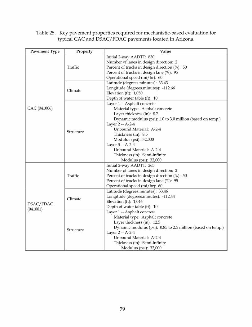
79
Table 25. Key pavement properties required for mechanistic-based evaluation for typical CAC and DSAC/FDAC pavements located in Arizona.
Pavement Type Property Value
Traffic
Initial 2-way AADTT: 830 Number of lanes in design direction: 2 Percent of trucks in design direction (%): 50 Percent of trucks in design lane (%): 95 Operational speed (mi/hr): 60
Climate
Latitude (degrees.minutes): 33.43 Longitude (degrees.minutes): -112.66 Elevation (ft): 1,050 Depth of water table (ft): 10
CAC (041006)
Structure
Layer 1 -- Asphalt concrete Material type: Asphalt concrete Layer thickness (in): 8.7 Dynamic modulus (psi): 1.0 to 3.0 million (based on temp.) Layer 2 -- A-2-4 Unbound Material: A-2-4 Thickness (in): 8.5 Modulus (psi): 32,000 Layer 3 -- A-2-4 Unbound Material: A-2-4 Thickness (in): Semi-infinite Modulus (psi): 32,000
Traffic
Initial 2-way AADTT: 265 Number of lanes in design direction: 2 Percent of trucks in design direction (%): 50 Percent of trucks in design lane (%): 95 Operational speed (mi/hr): 60
Climate
Latitude (degrees.minutes): 33.46 Longitude (degrees.minutes): -112.44 Elevation (ft): 1,046 Depth of water table (ft): 10 DSAC/FDAC
(041001)
Structure
Layer 1 -- Asphalt concrete Material type: Asphalt concrete Layer thickness (in): 12.5 Dynamic modulus (psi): 0.85 to 2.5 million (based on temp.) Layer 2 -- A-2-4 Unbound Material: A-2-4 Thickness (in): Semi-infinite Modulus (psi): 32,000

80
Table 26. Key pavement properties required for mechanistic-based evaluation for typical JPC pavements located in Arizona.
Pavement Type Property Value
Traffic
Initial 2-way AADTT: 1,895 Number of lanes in design direction: 2 Percent of trucks in design direction (%): 50 Percent of trucks in design lane (%): 95 Operational speed (mi/hr): 60
Climate
Latitude (degrees.minutes): 33.38 Longitude (degrees.minutes): -111.83 Elevation (ft): 1,190 Depth of water table (ft): 10
Structure
Layer 1 -- JPCP Material type: PCC Layer thickness (in): 13.0 28-day modulus of rupture (psi): 575 Layer 2 -- A-2-7 Unbound Material: A-2-7 Thickness (in): 6 Modulus (psi): 42,000 Layer 3 -- A-2-4 Unbound Material: A-7-6 Thickness (in): Semi-infinite Modulus (psi): 35,000
JPC (047613)
Design
Joint Design Joint spacing (ft): 13, 17 (mean = 15) Sealant type: Liquid Dowel diameter (in): None Edge Support Tied PCC shoulder Long-term LTE (%): 40 Widened Slab (ft): None Base Properties Base type: Granular Erodibility index: Erosion Resistant (3) Base/slab friction coefficient: 0.85 PCC-Base Interface: Unbonded
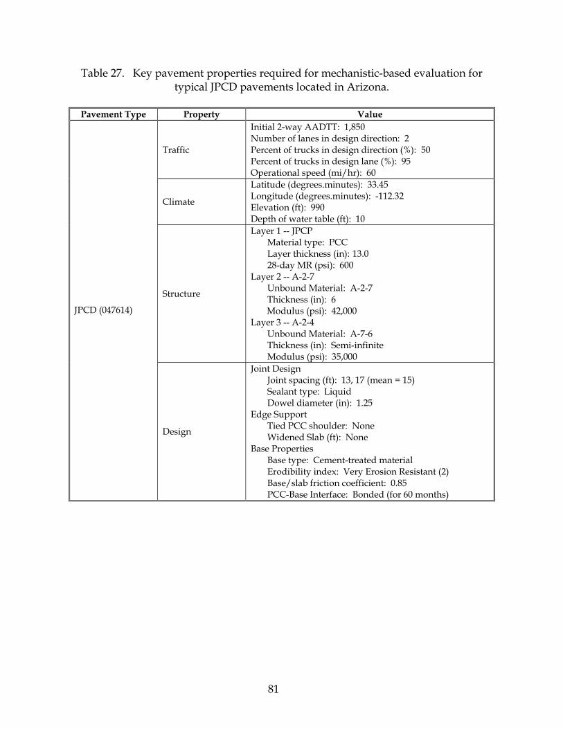
81
Table 27. Key pavement properties required for mechanistic-based evaluation for typical JPCD pavements located in Arizona.
Pavement Type Property Value
Traffic
Initial 2-way AADTT: 1,850 Number of lanes in design direction: 2 Percent of trucks in design direction (%): 50 Percent of trucks in design lane (%): 95 Operational speed (mi/hr): 60
Climate
Latitude (degrees.minutes): 33.45 Longitude (degrees.minutes): -112.32 Elevation (ft): 990 Depth of water table (ft): 10
Structure
Layer 1 -- JPCP Material type: PCC Layer thickness (in): 13.0 28-day MR (psi): 600 Layer 2 -- A-2-7 Unbound Material: A-2-7 Thickness (in): 6 Modulus (psi): 42,000 Layer 3 -- A-2-4 Unbound Material: A-7-6 Thickness (in): Semi-infinite Modulus (psi): 35,000
JPCD (047614)
Design
Joint Design Joint spacing (ft): 13, 17 (mean = 15) Sealant type: Liquid Dowel diameter (in): 1.25 Edge Support Tied PCC shoulder: None Widened Slab (ft): None Base Properties Base type: Cement-treated material Erodibility index: Very Erosion Resistant (2) Base/slab friction coefficient: 0.85 PCC-Base Interface: Bonded (for 60 months)

82
Table 28. Key pavement properties required for mechanistic-based evaluation for typical CRC pavements located in Arizona.
Pavement Type Property Value
Traffic
Initial 2-way AADTT: 1,770 Number of lanes in design direction: 2 Percent of trucks in design direction (%): 50 Percent of trucks in design lane (%): 77 Operational speed (mi/hr): 60
Climate
Latitude (degrees.minutes): 33.6 Longitude (degrees.minutes): -112.25 Elevation (ft): 1,151 Depth of water table (ft): 10
Structure
Layer 1 -- CRCP Material type: PCC Layer thickness (in): 9.0 28-day compressive strength (psi): 5,654 Layer 2 -- Asphalt Material: Asphalt Thickness (in): 4 Modulus (psi): 0.5 to 1.2 million (based on temp.) Layer 3 -- A-2-4 Unbound Material: A-6 Thickness (in): Semi-infinite Modulus (psi): 17,000
CRC (047079)
Design
Steel Reinforcement Percent steel (%): 0.57 Bar diameter (in): 0.63 Steel depth (in): 4.5 Edge Support AC shoulder Base Properties Base type: Granular Erodibility index: Erosion Resistant (3) Base/slab friction coefficient: 7.6

83
Figure 45. Predicted versus measured cracking (longitudinal and fatigue) for CAC at SHRP site 041006 (I-10, Maricopa County, MP 110.65).
0
0.01
0.02
0.03
0.04
0.05
0.06
0.07
0.08
0 0.01 0.02 0.03 0.04 0.05 0.06 0.07 0.08
Measured transverse joint faulting, in
Pre
dict
ed tr
ansv
erse
join
t fau
lting
, in
Figure 46. Predicted versus measured transverse joint faulting for JPC at SHRP site
047613 (SR 360, Maricopa County, MP 7.42).
0
1
2
3
4
5
6
0 1 2 3 4 5 6Measured cracking, percent
Pre
dict
ed c
rack
ing,
per
cent
R2 = 0.70N = 10

84
The ranges of key pavement parameters (i.e., surface layer thickness, traffic, and subgrade properties) used in developing the “typical” pavements are presented in table 29. The information in this table was used to develop a typical sample of pavements that cover the range of traffic application, the range of pavement surface layer thickness, three climate zones, and a single subgrade type. The CAC and DSAC/FDAC pavements were evaluated over a 25-year period while JPC, JPCD, and CRC pavements were evaluated over a 35-year period. Performance indicators along with terminal values based on facility type (i.e., Interstate and Non-Interstates) used in analysis to determine service life are summarized in table 30. Pavements that did not experience terminal levels of distress or smoothness at the end of the evaluation period were censored as done typically in survival analyses. Perform M-E Evaluation of “Typical” Pavements and Determine Pavement Service Life Results of the mechanistic-based evaluations of the “typical” pavements are presented in tables 31 through 35. M-E Performance Analysis Results Survival analysis was performed using data obtained from the M-E evaluation of “typical” pavements. The survival analysis assumed that the sample of data (as provided in these tables) was generally typical of a subset of Arizona pavements in terms of design, climate, traffic, soils, and materials. The overall results of the M-E analysis are presented in table 36 and a comparison of survival life estimated in terms of pavement age in years are plotted in figures 47 and 48. With the exception of the JPCD and CRC life estimates, these figures show a reasonable comparison between actual and simulated estimates of survival life for both flexible and rigid pavements. The survival estimates shown in figure 48 for JPCD and CRC are minimum values; median life estimates were not available due to no failures with these pavements.

85
Table 29. Typical range of surface layer thickness, traffic, and subgrade properties used in developing “typical” pavements.
Pavement Type Pavement Characteristic Variable Range
Thickness, in 4 to 8 Traffic, trucks applied per year, millions 0.25 to 1.0 CAC Subgrade, AASHTO soil class A-2-4 Thickness, in 9 to 13 Traffic, trucks applied per year, millions 0.25 to 1.05 DSAC/FDAC Subgrade, AASHTO soil class A-2-4 Thickness, in 8 to 13 Traffic, trucks applied per year, millions 0.5 to 1.5 JPC Subgrade, AASHTO soil class A-7-6 Thickness, in 10 to 13 Traffic, trucks applied per year, millions 3.2 to 5.5 JPCD Subgrade, AASHTO soil class A-7-6 Thickness, in 8 to 13 Traffic, trucks applied per year, millions 0.5 to 2.5 CRC Subgrade, AASHTO soil class A-6
Table 30. Performance indicators along with terminal values based on facility type used in analysis.
Facility Type Pavement Type Performance Indicator
Interstate Non-Interstate Cracking (fatigue [alligator] and longitudinal cracking (percent area, all severities)
20 30
Rutting, in 0.625 0.90
CAC, DSAC/FDAC
Smoothness (IRI, in/mi) 150 200 Mean transverse joint faulting, in 0.13 0.20
Slab transverse cracking (percent slabs cracked, all severities)
15 25 JPC/JPCD
Smoothness (IRI, in/mi) 150 200 Punchouts, (no. per mile, all severities) 10 — CRC Smoothness (IRI, in/mi) 150 200
.
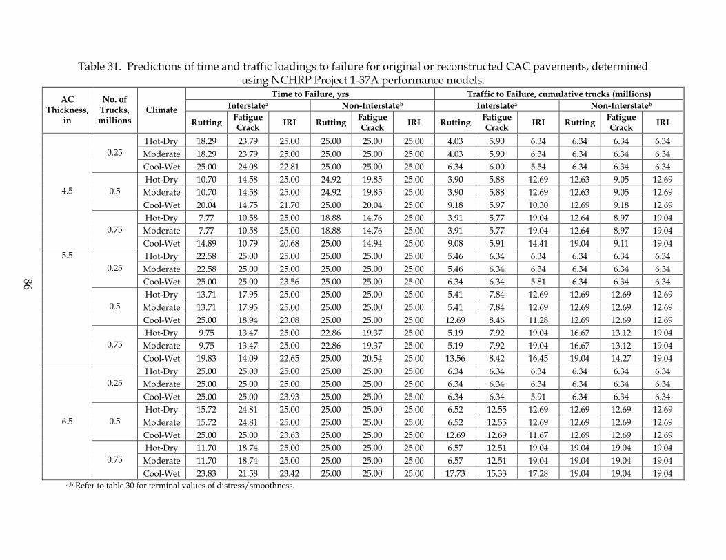
Table 31. Predictions of time and traffic loadings to failure for original or reconstructed CAC pavements, determined using NCHRP Project 1-37A performance models.
Time to Failure, yrs Traffic to Failure, cumulative trucks (millions) Interstatea Non-Interstateb Interstatea Non-Interstateb
AC Thickness,
in
No. of Trucks, millions
Climate Rutting Fatigue
Crack IRI Rutting Fatigue Crack IRI Rutting Fatigue
Crack IRI Rutting Fatigue Crack IRI
Hot-Dry 18.29 23.79 25.00 25.00 25.00 25.00 4.03 5.90 6.34 6.34 6.34 6.34 Moderate 18.29 23.79 25.00 25.00 25.00 25.00 4.03 5.90 6.34 6.34 6.34 6.34 0.25 Cool-Wet 25.00 24.08 22.81 25.00 25.00 25.00 6.34 6.00 5.54 6.34 6.34 6.34 Hot-Dry 10.70 14.58 25.00 24.92 19.85 25.00 3.90 5.88 12.69 12.63 9.05 12.69
Moderate 10.70 14.58 25.00 24.92 19.85 25.00 3.90 5.88 12.69 12.63 9.05 12.69 0.5 Cool-Wet 20.04 14.75 21.70 25.00 20.04 25.00 9.18 5.97 10.30 12.69 9.18 12.69 Hot-Dry 7.77 10.58 25.00 18.88 14.76 25.00 3.91 5.77 19.04 12.64 8.97 19.04
Moderate 7.77 10.58 25.00 18.88 14.76 25.00 3.91 5.77 19.04 12.64 8.97 19.04
4.5
0.75 Cool-Wet 14.89 10.79 20.68 25.00 14.94 25.00 9.08 5.91 14.41 19.04 9.11 19.04 Hot-Dry 22.58 25.00 25.00 25.00 25.00 25.00 5.46 6.34 6.34 6.34 6.34 6.34
Moderate 22.58 25.00 25.00 25.00 25.00 25.00 5.46 6.34 6.34 6.34 6.34 6.34 0.25 Cool-Wet 25.00 25.00 23.56 25.00 25.00 25.00 6.34 6.34 5.81 6.34 6.34 6.34 Hot-Dry 13.71 17.95 25.00 25.00 25.00 25.00 5.41 7.84 12.69 12.69 12.69 12.69
Moderate 13.71 17.95 25.00 25.00 25.00 25.00 5.41 7.84 12.69 12.69 12.69 12.69 0.5 Cool-Wet 25.00 18.94 23.08 25.00 25.00 25.00 12.69 8.46 11.28 12.69 12.69 12.69 Hot-Dry 9.75 13.47 25.00 22.86 19.37 25.00 5.19 7.92 19.04 16.67 13.12 19.04
Moderate 9.75 13.47 25.00 22.86 19.37 25.00 5.19 7.92 19.04 16.67 13.12 19.04
5.5
0.75 Cool-Wet 19.83 14.09 22.65 25.00 20.54 25.00 13.56 8.42 16.45 19.04 14.27 19.04 Hot-Dry 25.00 25.00 25.00 25.00 25.00 25.00 6.34 6.34 6.34 6.34 6.34 6.34
Moderate 25.00 25.00 25.00 25.00 25.00 25.00 6.34 6.34 6.34 6.34 6.34 6.34 0.25 Cool-Wet 25.00 25.00 23.93 25.00 25.00 25.00 6.34 6.34 5.91 6.34 6.34 6.34 Hot-Dry 15.72 24.81 25.00 25.00 25.00 25.00 6.52 12.55 12.69 12.69 12.69 12.69
Moderate 15.72 24.81 25.00 25.00 25.00 25.00 6.52 12.55 12.69 12.69 12.69 12.69 0.5 Cool-Wet 25.00 25.00 23.63 25.00 25.00 25.00 12.69 12.69 11.67 12.69 12.69 12.69 Hot-Dry 11.70 18.74 25.00 25.00 25.00 25.00 6.57 12.51 19.04 19.04 19.04 19.04
Moderate 11.70 18.74 25.00 25.00 25.00 25.00 6.57 12.51 19.04 19.04 19.04 19.04
6.5
0.75 Cool-Wet 23.83 21.58 23.42 25.00 25.00 25.00 17.73 15.33 17.28 19.04 19.04 19.04
a,b Refer to table 30 for terminal values of distress/smoothness.
86
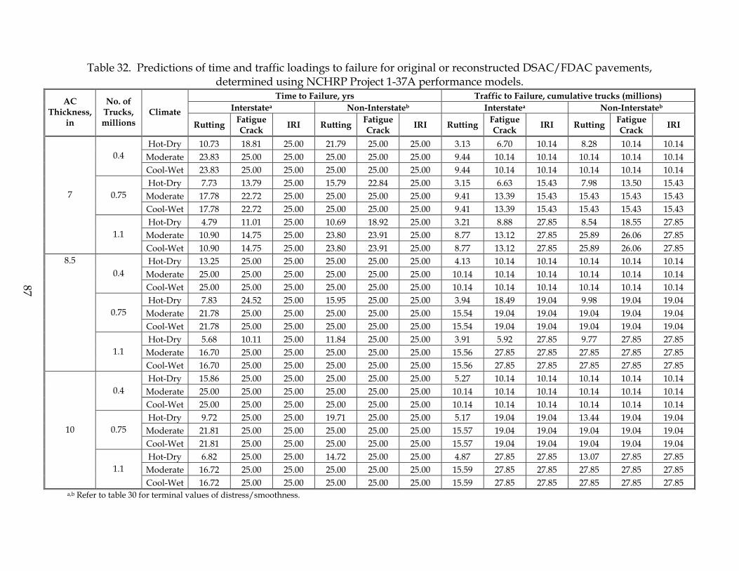
Table 32. Predictions of time and traffic loadings to failure for original or reconstructed DSAC/FDAC pavements, determined using NCHRP Project 1-37A performance models.
Time to Failure, yrs Traffic to Failure, cumulative trucks (millions) Interstatea Non-Interstateb Interstatea Non-Interstateb
AC Thickness,
in
No. of Trucks, millions
Climate Rutting Fatigue
Crack IRI Rutting Fatigue Crack IRI Rutting Fatigue
Crack IRI Rutting Fatigue Crack IRI
Hot-Dry 10.73 18.81 25.00 21.79 25.00 25.00 3.13 6.70 10.14 8.28 10.14 10.14 Moderate 23.83 25.00 25.00 25.00 25.00 25.00 9.44 10.14 10.14 10.14 10.14 10.14 0.4 Cool-Wet 23.83 25.00 25.00 25.00 25.00 25.00 9.44 10.14 10.14 10.14 10.14 10.14 Hot-Dry 7.73 13.79 25.00 15.79 22.84 25.00 3.15 6.63 15.43 7.98 13.50 15.43
Moderate 17.78 22.72 25.00 25.00 25.00 25.00 9.41 13.39 15.43 15.43 15.43 15.43 0.75 Cool-Wet 17.78 22.72 25.00 25.00 25.00 25.00 9.41 13.39 15.43 15.43 15.43 15.43 Hot-Dry 4.79 11.01 25.00 10.69 18.92 25.00 3.21 8.88 27.85 8.54 18.55 27.85
Moderate 10.90 14.75 25.00 23.80 23.91 25.00 8.77 13.12 27.85 25.89 26.06 27.85
7
1.1 Cool-Wet 10.90 14.75 25.00 23.80 23.91 25.00 8.77 13.12 27.85 25.89 26.06 27.85 Hot-Dry 13.25 25.00 25.00 25.00 25.00 25.00 4.13 10.14 10.14 10.14 10.14 10.14
Moderate 25.00 25.00 25.00 25.00 25.00 25.00 10.14 10.14 10.14 10.14 10.14 10.14 0.4 Cool-Wet 25.00 25.00 25.00 25.00 25.00 25.00 10.14 10.14 10.14 10.14 10.14 10.14 Hot-Dry 7.83 24.52 25.00 15.95 25.00 25.00 3.94 18.49 19.04 9.98 19.04 19.04
Moderate 21.78 25.00 25.00 25.00 25.00 25.00 15.54 19.04 19.04 19.04 19.04 19.04 0.75 Cool-Wet 21.78 25.00 25.00 25.00 25.00 25.00 15.54 19.04 19.04 19.04 19.04 19.04 Hot-Dry 5.68 10.11 25.00 11.84 25.00 25.00 3.91 5.92 27.85 9.77 27.85 27.85
Moderate 16.70 25.00 25.00 25.00 25.00 25.00 15.56 27.85 27.85 27.85 27.85 27.85
8.5
1.1 Cool-Wet 16.70 25.00 25.00 25.00 25.00 25.00 15.56 27.85 27.85 27.85 27.85 27.85 Hot-Dry 15.86 25.00 25.00 25.00 25.00 25.00 5.27 10.14 10.14 10.14 10.14 10.14
Moderate 25.00 25.00 25.00 25.00 25.00 25.00 10.14 10.14 10.14 10.14 10.14 10.14 0.4 Cool-Wet 25.00 25.00 25.00 25.00 25.00 25.00 10.14 10.14 10.14 10.14 10.14 10.14 Hot-Dry 9.72 25.00 25.00 19.71 25.00 25.00 5.17 19.04 19.04 13.44 19.04 19.04
Moderate 21.81 25.00 25.00 25.00 25.00 25.00 15.57 19.04 19.04 19.04 19.04 19.04 0.75 Cool-Wet 21.81 25.00 25.00 25.00 25.00 25.00 15.57 19.04 19.04 19.04 19.04 19.04 Hot-Dry 6.82 25.00 25.00 14.72 25.00 25.00 4.87 27.85 27.85 13.07 27.85 27.85
Moderate 16.72 25.00 25.00 25.00 25.00 25.00 15.59 27.85 27.85 27.85 27.85 27.85
10
1.1 Cool-Wet 16.72 25.00 25.00 25.00 25.00 25.00 15.59 27.85 27.85 27.85 27.85 27.85
a,b Refer to table 30 for terminal values of distress/smoothness.
87

Table 33. Predictions of time and traffic loadings to failure for original or reconstructed JPC pavements, determined using NCHRP Project 1-37A performance models.
Time to Failure, yrs Traffic to Failure, cumulative trucks (millions) Interstatea Non-Interstateb Interstatea Non-Interstateb
PCC Thickness,
in
No. of Trucks, millions
Climate Crack Fault IRI Crack Fault IRI Crack Fault IRI Crack Fault IRI
Hot-Dry 18.25 25.79 24.17 14.25 35.00 35.00 6.78 11.22 10.19 10.24 17.96 17.96 Moderate 18.55 18.42 19.67 24.63 35.00 33.05 6.94 10.48 7.54 10.48 17.96 16.42 0.5 Cool-Wet 16.08 34.46 19.54 21.58 35.00 29.14 5.68 17.52 7.47 8.63 17.96 13.51 Hot-Dry 10.42 16.17 14.73 14.21 28.87 24.75 6.24 11.22 9.88 9.40 26.12 20.70
Moderate 10.52 11.21 12.11 14.53 25.54 22.25 6.32 6.85 7.59 9.69 21.70 17.69 1.0 Cool-Wet 8.86 22.21 14.26 12.51 35.00 21.46 5.08 17.64 9.45 7.93 35.23 16.79 Hot-Dry 6.83 11.96 10.59 9.75 21.96 18.50 5.57 11.27 9.63 8.65 26.19 20.47
Moderate 7.08 8.12 8.58 10.03 19.29 16.56 5.81 6.88 7.37 8.97 21.72 17.53
9
1.5 Cool-Wet 5.95 16.54 10.88 8.56 35.00 17.95 4.71 17.49 9.96 7.35 53.18 19.61 Hot-Dry 35.00 35.00 35.00 35.00 35.00 35.00 17.96 17.96 17.96 17.96 17.96 17.96
Moderate 35.00 35.00 35.00 35.00 35.00 35.00 17.96 17.96 17.96 17.96 17.96 17.96 0.5 Cool-Wet 35.00 35.00 35.00 35.00 35.00 35.00 17.96 17.96 17.96 17.96 17.96 17.96 Hot-Dry 35.00 29.71 35.00 35.00 35.00 35.00 35.23 27.29 35.23 35.23 35.23 35.23
Moderate 35.00 24.50 31.08 35.00 35.00 35.00 35.23 20.40 29.27 35.23 35.23 35.23 1.0 Cool-Wet 35.00 35.00 30.25 35.00 35.00 35.00 35.23 35.23 28.06 35.23 35.23 35.23 Hot-Dry 35.00 22.58 28.55 35.00 35.00 35.00 53.18 27.30 38.79 53.18 53.18 53.18
Moderate 35.00 35.00 35.00 35.00 35.00 35.00 53.18 53.18 53.18 53.18 53.18 53.18
11
1.5 Cool-Wet Hot-Dry 35.00 35.00 35.00 35.00 35.00 35.00 17.96 17.96 17.96 17.96 17.96 17.96
Moderate 35.00 35.00 35.00 35.00 35.00 35.00 17.96 17.96 17.96 17.96 17.96 17.96 0.5 Cool-Wet 35.00 35.00 35.00 35.00 35.00 35.00 17.96 17.96 17.96 17.96 17.96 17.96 Hot-Dry 35.00 35.00 35.00 35.00 35.00 35.00 35.23 35.23 35.23 35.23 35.23 35.23
Moderate 35.00 35.00 35.00 35.00 35.00 35.00 35.23 35.23 35.23 35.23 35.23 35.23 1.0 Cool-Wet 35.00 35.00 35.00 35.00 35.00 35.00 35.23 35.23 35.23 35.23 35.23 35.23 Hot-Dry 35.00 35.00 35.00 35.00 35.00 35.00 53.18 53.18 53.18 53.18 53.18 53.18
Moderate 35.00 35.00 35.00 35.00 35.00 35.00 53.18 53.18 53.18 53.18 53.18 53.18
13
1.5 Cool-Wet 35.00 35.00 35.00 35.00 35.00 35.00 53.18 53.18 53.18 53.18 53.18 53.18
a,b Refer to table 30 for terminal values of distress/smoothness.
88
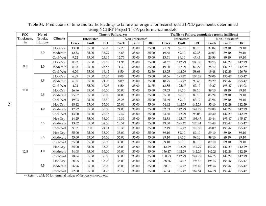
Table 34. Predictions of time and traffic loadings to failure for original or reconstructed JPCD pavements, determined using NCHRP Project 1-37A performance models.
Time to Failure, yrs Traffic to Failure, cumulative trucks (millions) Interstatea Non-Interstateb Interstatea Non-Interstateb
PCC Thickness,
in
No. of Trucks, millions
Climate Crack Fault IRI Crack Fault IRI Crack Fault IRI Crack Fault IRI
Hot-Dry 13.00 35.00 35.00 17.25 35.00 35.00 21.09 89.10 89.10 31.07 89.10 89.10 Moderate 12.33 35.00 33.29 16.83 35.00 35.00 19.68 89.10 82.38 30.03 89.10 89.10 2.5 Cool-Wet 9.22 35.00 23.15 12.75 35.00 35.00 13.51 89.10 47.43 20.56 89.10 89.10 Hot-Dry 8.92 35.00 29.05 11.96 35.00 35.00 20.67 142.29 106.55 30.15 142.29 142.29
Moderate 8.33 35.00 25.85 11.33 35.00 35.00 19.00 142.29 89.27 28.12 142.29 142.29 4.0 Cool-Wet 6.20 35.00 19.42 8.50 35.00 32.50 13.25 142.29 58.68 19.48 142.29 126.70 Hot-Dry 6.89 35.00 23.33 9.08 35.00 35.00 20.66 195.47 105.28 29.06 195.47 195.47
Moderate 6.35 35.00 21.03 8.89 35.00 35.00 18.75 195.47 90.43 28.29 195.47 195.47
9.5
5.5 Cool-Wet 4.92 35.00 17.07 6.50 35.00 28.75 13.85 195.47 67.17 19.27 195.47 144.03 Hot-Dry 26.96 35.00 35.00 35.00 35.00 35.00 59.53 89.10 89.10 89.10 89.10 89.10
Moderate 25.67 35.00 35.00 34.03 35.00 35.00 55.30 89.10 89.10 85.24 89.10 89.10 2.5 Cool-Wet 19.03 35.00 33.50 25.25 35.00 35.00 35.69 89.10 83.19 53.96 89.10 89.10 Hot-Dry 18.42 35.00 35.00 25.04 35.00 35.00 54.42 142.29 142.29 85.10 142.29 142.29
Moderate 17.92 35.00 35.00 24.00 35.00 35.00 52.33 142.29 142.29 79.88 142.29 142.29 4.0 Cool-Wet 13.00 35.00 27.15 17.42 35.00 35.00 33.68 142.29 96.08 50.30 142.29 142.29 Hot-Dry 14.25 35.00 35.00 19.39 35.00 35.00 52.38 195.47 195.47 80.44 195.47 195.47
Moderate 13.62 35.00 32.06 18.54 35.00 35.00 49.30 195.47 170.44 75.48 195.47 195.47
11.0
5.5 Cool-Wet 9.92 5.00 24.11 13.38 35.00 35.00 32.49 195.47 110.50 48.09 195.47 195.47 Hot-Dry 35.00 35.00 35.00 35.00 35.00 35.00 89.10 89.10 89.10 89.10 89.10 89.10
Moderate 35.00 35.00 35.00 35.00 35.00 35.00 89.10 89.10 89.10 89.10 89.10 89.10 2.5 Cool-Wet 35.00 35.00 35.00 35.00 35.00 35.00 89.10 89.10 89.10 89.10 89.10 89.10 Hot-Dry 35.00 35.00 35.00 35.00 35.00 35.00 142.29 142.29 142.29 142.29 142.29 142.29
Moderate 34.08 35.00 35.00 35.00 35.00 35.00 136.47 142.29 142.29 142.29 142.29 142.29 4.0 Cool-Wet 28.04 35.00 35.00 35.00 35.00 35.00 100.93 142.29 142.29 142.29 142.29 142.29 Hot-Dry 28.05 35.00 35.00 35.00 35.00 35.00 138.76 195.47 195.47 195.47 195.47 195.47
Moderate 26.96 35.00 35.00 35.00 35.00 35.00 130.61 195.47 195.47 195.47 195.47 195.47
12.5
5.5
Cool-Wet 22.00 35.00 31.75 29.17 35.00 35.00 96.54 195.47 167.84 147.24 195.47 195.47 a,b Refer to table 30 for terminal values of distress/smoothness.
89

Table 35. Predictions of time and traffic loadings to failure for original or reconstructed CRC pavements, determined using NCHRP Project 1-37A performance models.
Time to Failure, yrs Traffic to Failure, cumulative trucks (million) PCC Thickness, in
No of Trucks, million Climate
Punchouts IRI Punchouts IRI Hot-Dry 35.00 35.00 17.20 17.20
Moderate 35.00 35.00 17.20 17.20 0.5 Cool-Wet 35.00 35.00 17.20 17.20 Hot-Dry 28.47 35.00 24.96 34.41
Moderate 29.06 35.00 25.76 34.41 1.0 Cool-Wet 35.00 35.00 34.41 34.41 Hot-Dry 22.69 35.00 26.62 51.61
Moderate 23.30 35.00 27.69 61.61
9
1.5 Cool-Wet 31.54 35.00 43.85 51.61 Hot-Dry 35.00 35.00 17.20 17.20
Moderate 35.00 35.00 17.20 17.20 0.5 Cool-Wet 35.00 35.00 17.20 17.20 Hot-Dry 32.68 35.00 30.90 34.41
Moderate 33.33 35.00 31.86 34.41 1.0 Cool-Wet 35.00 35.00 34.41 34.41 Hot-Dry 26.54 35.00 33.66 51.61
Moderate 26.77 35.00 34.09 51.61
9.5
1.5 Cool-Wet 35.0 35.00 51.61 51.61 Hot-Dry 35.00 35.00 17.20 17.20
Moderate 35.00 35.00 17.20 17.20 0.5 Cool-Wet 35.00 35.00 17.20 17.20 Hot-Dry 35.00 35.00 34.41 34.41
Moderate 35.00 35.00 34.41 34.41 1.0 Cool-Wet 35.00 35.00 34.41 34.41 Hot-Dry 29.70 35.00 39.95 51.61
Moderate 30.55 35.00 41.74 51.61
10
1.5 Cool-Wet 35.00 35.00 51.61 51.61
a,b Refer to table 30 for terminal values of distress/smoothness.
90

91
Table 36. Survival analysis results of service life data obtained from M-E evaluation of “typical” pavements.
Pavement
Type Facility
Type Climate No. 50% Survival
Age, yrs 50% Survival Life,
No. of trucks (millions) CAC I Cool-Wet 9 19.34 8.11 CAC I Hot-Dry 9 15.32 5.33 CAC I Moderate 9 15.32 5.33 CAC NI Cool-Wet 9 28.07 15.23 CAC NI Hot-Dry 9 28.18 15.00 CAC NI Moderate 9 28.18 15.00
DSAC/FDAC I Cool-Wet 9 20.64 21.18 DSAC/FDAC I Hot-Dry 9 9.16 6.50 DSAC/FDAC I Moderate 9 20.64 21.18 DSAC/FDAC NI Cool-Wet 9 27.53 28.61 DSAC/FDAC NI Hot-Dry 9 18.55 10.55 DSAC/FDAC NI Moderate 9 27.53 28.61
JPCD I Cool-Wet 9 16.35 104.68 JPCD I Hot-Dry 9 22.20 150.50 JPCD I Moderate 9 20.62 144.49 JPCD NI Cool-Wet 9 21.83 151.18 JPCD NI Hot-Dry 9 29.91 209.87 JPCD NI Moderate 9 27.29 238.36 JPC I Cool-Wet 9 33.21 53.28 JPC I Hot-Dry 9 30.81 56.34 JPC I Moderate 9 35.81 55.58 JPC NI Cool-Wet 9 40.52 54.39 JPC NI Hot-Dry 9 44.15 54.63 JPC NI Moderate 9 43.45 55.08 CRC I Cool-Wet 9 35.37 53.75 CRC I Hot-Dry 9 37.22 43.43 CRC I Moderate 9 37.04 42.34

92
Figure 47. Histogram showing 50 percent survival life estimated from ADOT performance data and M-E evaluation of typical ADOT flexible pavements.
Figure 48. Histogram showing 50 percent survival life estimated from ADOT performance data and M-E evaluation of typical ADOT rigid pavements.
0
5
10
15
20
25
30
CAC_I_ho
tdry
CAC_I_mod
erate
CAC_SU_c
ool
CAC_SU_h
otdry
CAC_SU_m
odera
te
DSFD_I_co
ol
DSFD_I_ho
tdry
DSFD_I_mod
erate
DSFD_SU_c
ool
DSFD_SU_h
otdry
DSFD_SU_m
odera
te
AZ PMS Data M-E Analysis
0
5
10
15
20
25
30
35
40
CRC_ISU_h
otdry
JPCD_IS
U_hotd
ry/mod
erate
JPC_IS
U_coo
lwet
JPC_IS
U_hotd
ry
AZ PMS DATA M-E Analysis

93
CHAPTER 4. ANALYSIS OF CONSTRUCTION COSTS INTRODUCTION One of the most critical aspects of LCCA is establishing the direct agency costs associated with building, maintaining, and rehabilitating the subject pavement types. Having the best unit price estimates possible for the various pay items associated with initial construction and periodic upkeep goes a long way toward ensuring a fair assessment of life cycle costs. To conduct the pavement LCCAs in this study, unit cost data from multiple sources were collected and carefully analyzed. Best estimates were then developed covering a range of initial pavement structure types (e.g., CAC, JPCD) and M&R treatments. This chapter discusses the process used to assess unit costs and presents the resulting best estimates used later in the LCCAs. DEVELOPMENT OF BEST ESTIMATES OF COSTS Sources of Data Three sources of unit cost data were tapped for the cost analysis. These sources are as follows:
• 1999 Construction Costs report prepared by the ADOT Contracts and Specifications Section.
• 2002 report “Arizona Asphalt Rubber Projects, 1988-2001” prepared by the ADOT Materials Group Pavement Design Section.
• ADOT 1999 Pavement Management Cost Estimate. Since the sources of unit cost data were available only in hard copy form, the data were manually entered into a Microsoft® Excel spreadsheet for subsequent analysis. The entered costs were then carefully checked and corrected, as necessary, to ensure the highest level of confidence in the resulting best estimates. Costs from the first source consisted of the three lowest contractor bid prices for pay items associated with projects put to bid in 1999. Data for over 100 different pavement-related pay items were extracted from this source and entered into a Microsoft® Excel spreadsheet for subsequent analysis. Table 37 provides a sample of the data collected and used in the study.

94
Table 37. Sample data obtained from Construction Costs report (ADOT, 1999).
Pay Item 2020085 Remove Bituminous Pavement (Milling, 3 in)
3 Low Bidders-Unit Price Quantity No. 1 No. 2 No. 3
Route
County
MP
Project
Project Location
5,530 $4.00 $3.00 $2.00 U 093 YV 172 H430601C NB & SB climbing lanes, MP 173-176 7,000 $2.50 $3.44 $ S 089 CN 549 H421501C Colorado River – State Line 3,627 $3.00 $3.00 $3.50 S 089A YV 353 H434201C Main Street Intersection, Cottonwood 4,890 $3.00 $2.50 $ S 080 CH 342 H4229C01 Jct. SR92 – Jct. Double Adobe Road
117,333 $0.82 $0.80 $1.25 I 015 MO 008 H4532C01 Littlefield – Virgin River 361 $1.80 $2.50 $1.00 I 040 AP 318 H4433C01 Pinta T I- McCarrell TI
1,222 $1.30 $0.75 $ I 010 PN 208 H4426C01 Picacho – Picacho Peak 181,529 $1.00 $1.00 $0.95 S 089 YV 338 H4541C01 Paulden – Hells Canyon 68,000 $0.80 $0.85 $1.10 S 066 MO 057 H4559C01 Thompson Avenue – AT Railway 17,100 $1.80 $1.80 $2.25 U 060 MA 160 H5405C01 US 60, Grand Avenue/27th Avenue
Costs from the second source consisted of first-bid mix and binder unit costs for asphalt rubber projects constructed between 1988 and 2001. The asphalt rubber projects included those that used dense-graded mixes (AR) or open-graded friction courses (FR) as part of the construction/resurfacing work. Table 38 provides a sample of the asphalt rubber cost data collected and used. Costs from the third source consisted of average in-place estimates for a variety of pavement activities, such as milling, application of a chip seal coat, and application of an asphalt rubber friction course (FR). These costs are used by ADOT pavement managers in developing preliminary cost estimates for future projects. Analysis of 1999 Construction Costs To begin this analysis, the average unit price of the three lowest contractors’ bids for each project for each pavement-related pay item were calculated. Next, the average costs were adjusted for inflation to 2003 prices using the following formula and a 2 percent inflation rate: $F = $P * (1 + i)n Eq. 8 where: $F = Current year (1999) cost adjusted for inflation, $. $P = Past year cost, $. i = Inflation rate, decimal (0.02) n = Number of years between 2003 and 1999 (4 years).

95
Table 38. Sample data obtained from Asphalt Rubber Projects report (ADOT, 2002).
TRACS
Project Name
Route
Beginning MP
End MP
Ton Mix
First-Bid Mix, $/ton
Ton Binder
First-Bid Binder,
$/ton H453201C Littlefield - Virgin River 015 7.94 13.12 26,770 $12.65 2,142 $230.50
H421201C Coconino National Forest Boundary - Buffalo Range TI 040 217.85 224.70 19,228 $26.00 1,601 $230.00
H443301C Pinta TI – McCarrel TI 040 318.80 330.60 62,698 $20.50 5,016 $210.00 H422801C Andy Devine Avenue 040B 52.75 56.40 20,025 $24.00 1,602 $290.00 H455901C Thompson Avenue – AT Railway 066 57.70 61.50 20,800 $23.00 1,665 $225.00 H453901C Mendocino Drive – Walker Road 069 286.80 292.84 34,274 $20.47 2,742 $202.28
H422201C Coyote Wash – East Boundary San Carlos 070 287.40 300.10 27,019 $18.00 2,162 $225.00
H422901C Jct. SR 92 – Jct. Double Adobe Road 080 343.59 347.40 8,530 $29.75 683 $275.00
H455501C Patagonia Lake Road – East Patagonia 082 12.30 20.60 21,470 $30.00 1,718 $270.00
H470501C Lenox Park – Deadman Flat 089 218.60 230.20 8,521 $23.00 682 $250.00 H384501C Long House Valley – Kayenta 160 372.50 389.50 38,985 $31.00 3,120 $250.00 H422601C Jct. SR 69 – Jct. I-17 169 0.00 4.65 34,860 $15.00 2,790 $200.00 H444501C Double Adobe – Elfrida 191 4.19 23.48 49,000 $18.00 3,920 $235.00 H456001C Thompson Road – Sunizona 191 27.00 38.60 21,710 $22.00 1,737 $270.00 H396001C Beaver Head Lodge – Jct. US 180 191 239.00 253.70 27,891 $29.00 2,231 $290.00
The average and standard deviation of the inflation-adjusted costs for each pay item were then calculated to give a preliminary indication of costs. These values are listed in table 39. Average and standard deviation costs were also determined based on the quantity of an item used on a project. The statistics were calculated in this manner so that it could be determined whether the cost of an item changed based on the quantity required for the project. As expected, the average inflation-adjusted unit cost of a pay item generally decreased with increasing quantity. Some example histograms that show these trends for a couple pay items are illustrated in figures 49 and 50. Also, as expected, the variability of the data decreased as the quantity of the item increased. Therefore, consideration had to be given to the size of the project when developing best estimates for the mean and standard deviation cost of individual pay items. Using selected minimum quantities for each pay item, small projects with higher-than usual costs were filtered out of analysis, allowing the average and standard deviation unit costs in table 39 to be recomputed. The resulting inflation-adjusted and quantity-filtered costs are provided in table 40.

96
Table 39. Inflation-adjusted unit costs for pay items in 1999 Construction Costs report (based on average of three lowest bid prices).
2003 Unit Cost (inflated from 1999) Material/
Activity Code Pay Item
No. Pay Item Description Unit No.
Average Std. Deviation 2020029 Removal of AC pavement yd2 38 $5.99 $4.98 2020030 Removal of AC pavement yd2 20 $2.01 $1.87 2020080 Remove bit. pvt. (milling, 0.5 in) yd2 5 $0.54 $0.16 2020081 Remove bit. pvt. (milling, 1 in) yd2 2 $0.76 $0.00 2020083 Remove bit. pvt. (milling, 2 in) yd2 12 $1.62 $1.03 2020084 Remove bit. pvt. (milling, 2.5 in) yd2 7 $2.35 $1.88 2020085 Remove bit. pvt. (milling, 3 in) yd2 10 $2.11 $1.03 2020086 Remove bit. pvt. (milling, 3.5 in) yd2 1 $1.06 — 2020087 Remove bit. pvt. (milling, 4 in) yd2 5 $2.20 $0.76
2020088 Remove bit. pvt. (milling, 4.5 to 6 in) yd2 5 $1.42 $0.32
RE
2020089 Remove bit. pvt. (milling, 6 to 8 in) yd2 2 $2.72 $1.16 3010001 Lime-treated subgrade yd2 2 $1.43 $0.33 3010011 Hydrated lime for subgrade treat. ton 1 $86.96 —
LS
3010012 Quicklime for subgrade treat. ton 1 $105.72 — 302???? Cement-treated subgrade yd2 0 — — CS 302???? Cement for subgrade treat. ton 0 — —
SM, SB 3030026 Aggregate subbase, class 6 yd3 4 $23.84 $13.70 3030022 Aggregate base, class 2 yd3 51 $35.70 $15.99 AB, OA 3030023 Aggregate base, class 3 yd3 12 $34.26 $17.05
CB 304???? Cement-treated base ton 0 — — CL 305???? Lean concrete base yd2 0 — —
4010010 PCC pavement (10 in) yd2 5 $31.70 $15.26 4010012 PCC pavement (12 in) yd2 2 $20.88 $0.06 4010013 PCC pavement (13 in) yd2 2 $51.60 $11.23 4010015 PCC pavement (15 in) yd2 2 $63.86 $2.55 4010016 PCC pavement (16 in) yd2 3 $74.74 $59.24
PC, PD
4010301 Load transfer dowels each 1 $19.12 — PR 4010039 PCC pavement (reinforced, 9 in) yd2 1 $36.08 —
4020060 Seal cracks in PCC pavement ft 2 $2.43 $0.65 4020061 Seal edge of PCC pavement ft 2 $0.95 $0.09
GR 4020048 Grind existing PCC pavement yd2 2 $37.60 $36.68 GV 4020080 Groove PCC pavement yd2 1 $2.62 — ?? 4020072 Repair PCC spalled areas ft2 3 $46.05 $49.22 ?? 4020090 PCC pavement slab repair yd2 2 $336.64 $182.16
4040125 Fog coat ton 37 $380.84 $273.23 4040126 Fog coat (ERA-25) ton 8 $333.24 $218.62
FL
4040163 Blotter material ton 53 $48.43 $85.61 4040074 Emulsified asphalt (CRS-2) ton 12 $297.34 $347.38 SC 4040162 Cover material yd3 11 $78.38 $68.94
Prime Coat 4040101 Prime coat ton 5 $293.15 $96.86 4040111 Bituminous tack coat ton 64 $172.37 $31.64 Tack Coat 4040116 Apply bituminous tack coat hour 70 $121.69 $31.28

97
Table 39. Inflation-adjusted unit costs for pay items in 1999 Construction Costs report
(based on average of three lowest bid prices) (continued).
2003 Unit Cost (inflated from 1999) Material/ Activity Code
Pay Item No.
Pay Item Description Unit No. Average Std. Deviation
4040262 Asphalt binder (PG 64-16) ton 14 $151.20 $8.95 4040264 Asphalt binder (PG 64-22) ton 10 $163.88 $12.70 4040270 Asphalt binder (PG 70-10) ton 11 $149.08 $8.43 4040272 Asphalt binder (PG 70-16) ton 4 $150.32 $7.76 4040280 Asphalt binder (PG 76-10) ton 8 $148.20 $8.03 4040282 Asphalt binder (PG 76-16) ton 4 $160.81 $31.90 4060008 AC (0.75-in mix) ton 3 $21.58 $2.53 4060015 AC (0.5-in mix) ton 2 $22.86 $1.96 4060021 AC (base mix) ton 1 $19.66 — 4060024 Mineral admixture (for 0.5-in mix) ton 2 $97.42 $0.00
4060026 Mineral admixture (for 0.75-in mix) ton 4 $97.42 $0.00
AC, LC, BB, OB
4060027 Mineral admixture ton 3 $97.42 $0.00 4070001 AC friction course (FC) mix ton 8 $34.99 $8.97 4070006 AC friction course (FC) mix ton 1 $33.19 —
FC
4070021 Mineral admixture (for FC mix) ton 7 $97.42 $0.00 RC 4080011 cold recycling (bit. surface) yd2 1 $1.32 —
4130040 Asphalt rubber AC mix (AR) ton 14 $26.33 $5.65
4130042 Asphalt rubber binder (for AR mix) ton 14 $265.98 $27.26
AR
4130044 Mineral admixture (for AR mix) ton 13 $97.42 $0.00
4140040 Asphalt rubber friction course (FR) mix ton 44 $32.71 $10.78
4140042 Asphalt rubber binder (for FR mix) ton 44 $300.85 $67.36
FR
4140044 Mineral admixture (for FR mix) ton 42 $97.42 $0.00 4160002 AC (0.75-in mix) (end product) ton 16 $27.18 $7.46 4160008 AC (base mix) (end product) ton 3 $18.59 $0.52 4160009 AC (end product) ton 4 $21.32 $5.81
AC (end product)
4160031 Mineral admixture ton 38 $97.42 $0.00

98
Figure 49. Unit cost histogram for pay item 3030022, class 2 aggregate base (AB) (based on 1999 Construction Costs report).
Figure 50. Unit cost histogram for pay item 4140040, asphalt rubber used in asphalt rubber friction course (FR) (based on data from 1999 Construction Costs report).
0.00
5.00
10.00
15.00
20.00
25.00
30.00
35.00
40.00
45.00
50.00
0 - 500 500 - 1,000 1,000 - 5,000 5,000 - 10,000 10,000 - 20,000 > 20,000
Quantity, yd3
Un
it C
ost
, $
Average Standard Deviation
0.00
10.00
20.00
30.00
40.00
50.00
60.00
70.00
0 - 500 500 - 1,000 1,000 - 5,000 5,000 - 10,000 10,000 - 20,000
Quantity, tons
Un
it C
ost
, $
Average Standard Deviation

99
Table 40. Inflation-adjusted and quantity-filtered unit costs for pay items in 1999
Construction Costs report (based on average of three lowest bid prices).
2003 Unit Cost (inflated from 1999 and filtered by quantity)
Material/ Activity Code
Pay Item No. Pay Item Description Unit Min.
Quantity No. Average Std. Deviation
2020029 Removal of AC pavement yd2 10,000 6 $1.23 $0.33 2020030 Removal of AC pavement yd2 10,000 15 $1.23 $0.66 2020080 Remove bit. pvt. (milling, 0.5 in) yd2 10,000 5 $0.54 $0.16 2020081 Remove bit. pvt. (milling, 1 in) yd2 10,000 1 $0.76 — 2020083 Remove bit. pvt. (milling, 2 in) yd2 10,000 10 $1.23 $0.36 2020084 Remove bit. pvt. (milling, 2.5 in) yd2 10,000 3 $1.25 $0.31 2020085 Remove bit. pvt. (milling, 3 in) yd2 10,000 4 $1.30 $0.54 2020086 Remove bit. pvt. (milling, 3.5 in) yd2 10,000 1 $1.06 — 2020087 Remove bit. pvt. (milling, 4 in) yd2 10,000 2 $1.50 $0.18
2020088 Remove bit. pvt. (milling, 4.5 to 6 in) yd2 10,000 5 $1.42 $0.32
RE
2020089 Remove bit. pvt. (milling, 6 to 8 in) yd2 10,000 1 $1.89 —
3010001 Lime-treated subgrade yd2 10,000 2 $1.43 $0.33
3010011 Hydrated lime for subgrade treat. ton 250 1 $86.96 —
LS
3010012 Quicklime for subgrade treat. ton 250 1 $105.72 — 302???? Cement-treated subgrade yd2 0 — — CS 302???? Cement for subgrade treat. ton 0 — —
SM, SB 3030026 Aggregate subbase, class 6 yd3 2,500 2 $17.32 $0.56 3030022 Aggregate base, class 2 yd3 2,500 16 $23.64 $5.26 AB, OA 3030023 Aggregate base, class 3 yd3 2,500 6 $23.77 $5.01
CB 304???? Cement treated base ton 0 — — CL 305???? Lean concrete base yd2 0 — —
4010010 PCC pavement (10 in) yd2 10,000 3 $20.60 $0.70 4010012 PCC pavement (12 in) yd2 10,000 2 $20.88 $0.06 4010013 PCC pavement (13 in) yd2 10,000 0 — — 4010016 PCC pavement (16 in) yd2 10,000 1 $26.12 —
PC, PD
4010301 Load transfer dowels each 5,000 0 — — PR 4010039 PCC pavement (reinforced, 9 in) yd2 10,000 0 — —
4020060 Seal cracks in PCC pavement ft 5,000 2 $2.43 $0.65 4020061 Seal edge of PCC pavement ft 10,000 2 $0.95 $0.09
GR 4020048 Grind existing PCC pavement yd2 10,000 1 $10.25 — GV 4020080 Groove PCC pavement yd2 10,000 1 $2.62 —
4020072 Repair PCC spalled areas ft2 1,000 1 $15.51 — 4020090 PCC pavement slab repair yd2 1,000 1 $207.83 —
4040125 Fog coat ton 10 23 $209.28 $32.04 4040126 Fog coat (ERA-25) ton 10 5 $239.64 $26.22
FL
4040163 Blotter material ton 50 31 $19.43 $7.77 4040074 Emulsified asphalt (CRS-2) ton 50 9 $180.37 $26.51 SC 4040162 Cover material yd3 500 6 $40.68 $7.58
Prime Coat 4040101 Prime coat ton 50 3 $222.79 $14.09 4040111 Bituminous tack coat ton 50 39 $163.44 $20.38 Tack Coat 4040116 Apply bituminous tack coat hour 50 53 $114.25 $24.50

100
Table 40. Inflation-adjusted and quantity-filtered unit costs for pay items in 1999
Construction Costs report (based on average of three lowest bid prices) (continued).
2003 Unit Cost (inflated from 1999 and filtered by quantity)
Material/ Activity Code
Pay Item No. Pay Item Description Unit Min.
Quantity No. Average Std. Deviation
4040262 Asphalt binder (PG 64-16) ton 500 7 $153.73 $9.61 4040264 Asphalt binder (PG 64-22) ton 500 9 $162.85 $13.02 4040270 Asphalt binder (PG 70-10) ton 500 10 $147.72 $7.50 4040272 Asphalt binder (PG 70-16) ton 500 4 $150.32 $7.76 4040280 Asphalt binder (PG 76-10) ton 500 7 $148.76 $8.51 4040282 Asphalt binder (PG 76-16) ton 500 2 $172.88 $47.79 4060008 AC (0.75-in mix) ton 1,000 3 $21.58 $2.53 4060015 AC (0.5-in mix) ton 1,000 2 $22.86 $1.96 4060021 AC (base mix) ton 2,500 1 $19.66 —
4060024 Mineral admixture (for 0.5-in mix) ton 25 1 $97.42 —
4060026 Mineral admixture (for 0.75-in mix) ton 25 4 $97.42 $0.00
AC, LC, BB, OB
4060027 Mineral admixture ton 100 3 $97.42 $0.00 4070001 AC friction course (FC) mix ton 2,500 3 $28.13 $3.65 FC 4070021 Mineral admixture (for FC mix) ton 25 5 $97.42 $0.00
RC 4080011 cold recycling (bit. surface) yd2 10,000 1 $1.32 — 4130040 Asphalt rubber AC mix (AR) ton 10,000 12 $25.65 $5.21
4130042 Asphalt rubber binder (for AR mix) ton 1,000 12 $260.48 $20.94
AR
4130044 Mineral admixture (for AR mix) ton 100 11 $97.42 $0.00
4140040 Asphalt rubber friction course (FR) mix ton 2,500 33 $29.44 $7.17
4140042 Asphalt rubber binder (for FR mix) ton 250 30 $274.99 $25.83
FR
4140044 Mineral admixture (for FR mix) ton 25 33 $97.42 $0.00 4160002 AC (0.75-in mix) (end product) ton 1,000 16 $27.18 $7.46 4160008 AC (base mix) (end product) ton 10,000 3 $18.59 $0.52 4160009 AC (end product) ton 10,000 4 $21.32 $5.81
AC (end product)
4160031 Mineral admixture ton 100 35 $97.42 $0.00
Analysis of Costs from Asphalt Rubber Projects Report As discussed previously, the costs associated with only four pay items were included in the Asphalt Rubber Projects report. These included the first-bid mix costs for asphalt rubber asphalt concrete (AR) and asphalt rubber asphalt concrete friction course (FR), as well as the binder costs (asphalt and asphalt rubber) for these two mixes. As with the 1999 construction costs, the costs from this source were inflated to 2003 prices using equation 8 at a 2 percent inflation rate. Similarly, the costs were subdivided by quantity to determine the effect of quantity on cost. Figures 51 through 54 are the resulting unit cost histograms for each pay item. They clearly show increased average costs and cost variations for small projects.
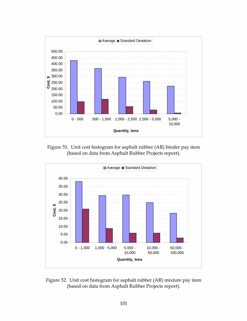
101
Figure 51. Unit cost histogram for asphalt rubber (AR) binder pay item (based on data from Asphalt Rubber Projects report).
Figure 52. Unit cost histogram for asphalt rubber (AR) mixture pay item (based on data from Asphalt Rubber Projects report).
0.00
50.00100.00
150.00200.00
250.00
300.00350.00
400.00450.00
500.00
0 - 500 500 - 1,000 1,000 - 2,500 2,500 - 5,000 5,000 -10,000
Quantity, tons
Cost
, $
Average Standard Deviation
0.00
5.00
10.00
15.00
20.00
25.00
30.00
35.00
40.00
0 - 1,000 1,000 - 5,000 5,000 -10,000
10,000 -50,000
50,000 -100,000
Quantity, tons
Cost
, $
Average Standard Deviation
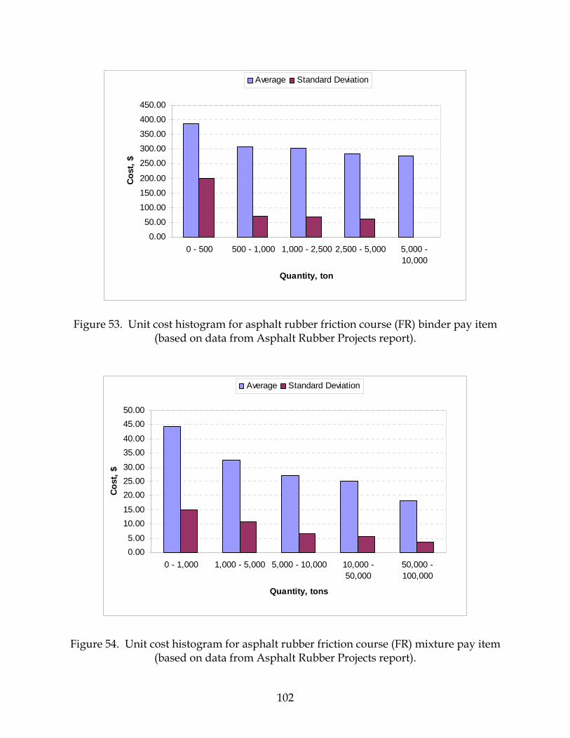
102
Figure 53. Unit cost histogram for asphalt rubber friction course (FR) binder pay item (based on data from Asphalt Rubber Projects report).
Figure 54. Unit cost histogram for asphalt rubber friction course (FR) mixture pay item
(based on data from Asphalt Rubber Projects report).
0.00
50.00
100.00
150.00
200.00
250.00
300.00
350.00
400.00
450.00
0 - 500 500 - 1,000 1,000 - 2,500 2,500 - 5,000 5,000 -10,000
Quantity, ton
Cos
t, $
Average Standard Deviation
0.005.00
10.0015.00
20.0025.0030.00
35.0040.00
45.0050.00
0 - 1,000 1,000 - 5,000 5,000 - 10,000 10,000 -50,000
50,000 -100,000
Quantity, tons
Cos
t, $
Average Standard Deviation

103
Using the same minimum quantities chosen to filter small projects in the analysis of 1999 construction costs, the average and standard deviation unit costs for AR and FR were computed. The resulting inflation-adjusted and quantity-filtered costs are provided in table 41. Analysis of Pavement Management Cost Estimates Table 42 shows the inflation-adjusted, in-place unit costs derived from the ADOT Pavement Management Cost Estimate. The costs represent base costs (i.e., engineering, traffic control, and other add-on costs not included). Summary of Unit Costs Table 43 summarizes the pay item unit costs derived from the three data sources considered in this study. As can be seen, there was generally good agreement among the three sources. For only a few pay items were there significant disparities in the mean unit costs. A major reason for the disparities was the low number of cost values (i.e., lack of projects and/or sizeable projects) available for some pay items. For the LCCAs conducted in chapter 7 of this report, pay item unit costs were assigned primarily using the inflation-adjusted and quantity-filtered costs from the 1999 Construction Costs report. If these costs were based on limited data (less than 5 data values) or were significantly different from the costs derived from the other data sources, then a best estimate was developed using the available information and engineering judgment. For pay items with no data available from any of the three sources, best estimates were developed solely using engineering judgment. A summary of the unit costs used in conducting the LCCAs is provided in chapter 7.

104
Table 41. Inflation-adjusted and quantity-filtered unit costs for pay items in Asphalt
Rubber Projects report (based on first-bid prices).
Activity Pay Item Designation
Activity Pay Item Description No. Average Standard
Deviation Asphalt rubber
(AR) mix 73 $24.61/ton $5.95/ton AR
Asphalt rubber binder (for AR) 66 $287.92/ton $62.30/ton
Asphalt rubber friction course 226 $27.78/ton $8.27/ton
FR Asphalt rubber binder (for FR) 220 $316.45/ton $74.27/ton
Table 42. Inflation-adjusted, in-place unit costs of various pay items contained in ADOT Pavement Management Cost Estimate.
2003 In-Place Unit Cost (inflated from 1999) Activity Pay Item
Designation
Activity Pay Item Description Overall Interstate Non-Interstate SC Chip seal coat 0.97/yd2 — 0.97/yd2 FC AC friction course (0.5 in) 1.52/yd2 1.19/yd2 1.19/yd2 RM Stress-absorbing membrane
interlayer (SAMI) 1.95/yd2 — —
Asphalt rubber AC 2.71/yd2 — — AR Asphalt rubber AC (2 in) 1.10/yd2 5.95/yd2 5.95/yd2
FR Asphalt rubber AC friction course (0.625 in)
2.38/yd2 1.95/yd2 1.95/yd2
Cold-recycle AC 0.87/yd2 — — RC AC-recycled 1.41/yd2 — — AC (0.75-in mix) 1.73/yd2 — — AC, BB AC (base mix) 1.41/yd2 — — Milling (0.75 in) 0.81/yd2 — — Milling (1 in) 1.08/yd2 — — Milling (2 in) 1.24/yd2 — — Milling (3 in) 1.35/yd2 — — Milling (4 in) 1.46/yd2 — —
RE
Milling (5 in) 1.57/yd2 — — GV Grooving PCC 3.25/yd2 — — GR Grinding PCC 6.49/yd2 — —

Table 43. Comparison of inflation-adjusted and quantity-filtered unit costs derived from various cost data sources.
Construction Costs Report Asphalt Rubber Report Activity Pay
Item Designation
Activity Pay Item Description No. Mean Std. Dev. Mean In-Place No. Mean Std. Dev. Mean In-Place
Pavement Management Cost
Estimates Fog Coat 28 $214.70/ton 32.84/ton FL
Blotter 31 $19.43/ton $7.77/ton $0.32/yd2
GV Grooving PCC 1 $2.62/yd2 — $2.62/yd2 $3.25/yd2 GV Grinding PCC 1 $10.25/yd2 — $10.25/yd2 $6.49/yd2
PCC crack sealing a 2 $2.43/ft $0.65/ft $2.43/ft PCC joint sealing (Long) 2 $0.95/ft $0.09/ft $0.95/ft
Emulsified asphalt (CRS-2) 9 $180.37/ton $26.51/ton SC Cover material 6 $40.68/yd3 $7.58/yd3
$0.49/yd2
$0.97/yd2
Repair PCC spalled areas 1 $15.51/ft2 — $15.51/ft2 PCC pavement slab repair 1 $207.83/yd2 — $207.83/yd2 Prime Coat 3 $222.79/ton $14.09/ton $0.09/yd2
Tack Coat 39 $163.44/ton $20.38/ton Apply Bituminous Tack Coat 53 $114.25/hr $24.50/hr
$0.10/yd2
AC friction course (0.5 in) 3 $28.13/ton $3.65/ton Asphalt binder (various grades) 39 $154.03/ton $13.93/ton
FC
Mineral admixture 5 $97.42/ton $0.00/ton 2.15/yd2
$1.52/yd2
RM Stress-absorbing membrane interlayer (SAMI) $1.95/yd2
Asphalt rubber (AR) mix 12 $25.65/ton $5.21/ton 73 $24.61/ton $5.95/ton Asphalt rubber binder (for AR) 12 $260.48/ton $20.94/ton 66 $287.92/ton $62.30/ton AR
Mineral admixture 11 $97.42/ton $0.00/ton 2.48/yd2
$2.50/yd2 $2.71/yd2
Asphalt rubber friction course (0.625 in) 33 $29.44/ton $7.17/ton 226 $27.78/ton $8.27/ton
Asphalt rubber binder (for FR) 30 $274.99/ton $25.83/ton 220 $316.45/ton $74.27/ton FR
Mineral admixture 33 $97.42/ton $0.00/ton
$2.61/yd2
$2.70/yd2 $2.38/yd2
Cold-recycle AC 1 $1.32/yd2 — $1.32/yd2 $0.87/yd2 RC AC-recycled $1.41/yd2
AC (0.5- and 0.75-in mixes) 5 $22.09/ton $2.16/ton Asphalt binder (various grades) 39 $154.03/ton $13.93/ton AC Mineral admixture (for 0.5- and
0.75-in mixes) 5 $97.42/ton $0.00/ton $1.66/yd2
$1.73/yd2
a Cost of this activity expected to be similar to cost of transverse PCC joint resealing.
105

Table 43. Comparison of inflation-adjusted and quantity-filtered unit costs derived from various cost data sources (continued).
Construction Costs Report Asphalt Rubber Report Activity Pay
Item Designation
Activity Pay Item Description No. Mean Std. Dev. Mean In-Place No. Mean Std. Dev. Mean In-Place
Pavement Management Cost
Estimates AC (base mix) 1 $19.66/ton —
Asphalt binder (various grades) 39 $154.03/ton $13.93/ton BB Mineral admixture 3 $97.42/ton $0.00/ton
$1.48/yd2
$1.41/yd2
PCC pavement (10 in) 3 $20.60//yd2 $0.70/yd2 $20.60/yd2 PCC pavement (12 in) 2 $20.88/yd2 $0.06/yd2 $20.88/yd2 PC PCC pavement (15 in) 1 $62.06/yd2 — $62.06/yd2 AC pavement removal 21 $1.23/yd2 $0.48/yd2 $1.23/yd2
Milling (0.5 in) 5 $0.54/yd2 $0.16/yd2 $0.54/yd2 Milling (0.75 in) $0.81/yd2
Milling (1 in) 1 $0.76/yd2 — $0.76/yd2 $1.08/yd2 Milling (2 in) 10 $1.23/yd2 $0.36/yd2 $1.23/yd2 $1.24/yd2
Milling (2.5 in) 3 $1.25/yd2 $0.31/yd2 $1.25/yd2 Milling (3 in) 4 $1.30/yd2 $0.54/yd2 $1.30/yd2 $1.35/yd2
Milling (3.5 in) 1 $1.06/yd2 — $1.06/yd2 Milling (4 in) 2 $1.50/yd2 $0.18/yd2 $1.50/yd2 $1.46/yd2
RE
Milling (4.5 to 6 in) 5 $1.42/yd2 $0.32/yd2 $1.42/yd2 $1.57/yd2
106
107
CHAPTER 5. USER COST BEST PRACTICES INTRODUCTION A review of current practices was made by the project team using information obtained through the Neutral Third Party (NTP) review of Ohio’s pavement type selection process and through collected literature on the topic of user costs (ERES, 2003). The review indicated that the user cost components that are predominately evaluated are the user delay costs resulting from traffic slowdowns and disruptions that occur during construction and maintenance operations. A secondary cost that is evaluated is the increased vehicle operating cost (VOC) that results from decreased smoothness. USER DELAY COSTS ASSOCIATED WITH WORK ZONES The process favored for evaluation of user delay costs is one presented by the Federal Highway Administration (FHWA) in their Interim Technical Bulletin on Life Cycle Cost Analysis in Pavement Design (Walls and Smith, 1998). This process was thoroughly evaluated in NCHRP Project 1-37A and has been adopted for use in the 2002 Pavement Design Guide. Two published reports reviewing the FHWA process were examined by the team. These reports, prepared for the Kentucky Transportation Cabinet (KTC) (Rister and Graves, 2002) and the Louisiana Department of Transportation and Development (DOTD) (Aghazadeh et al., 2003), provided favorable reviews of the FHWA procedure. The only other analysis approach that is currently being considered for use by State transportation agencies is the QuickZone User Delay Software developed by Mitretek for FHWA. QuickZone is a Microsoft® Excel spreadsheet application for estimating traffic delays that are the result of construction or maintenance operations. The QuickZone software is available from McTrans, which has reported the following capabilities of QuickZone:
• Quantifies corridor delay resulting from capacity decreases in work zones. • Identifies delay impacts of alternative construction phasing plans. • Supports trade-off analysis between construction costs and delay costs. • Considers alternate phasing schedules, such as location along mainline, time-of-
day (peak vs. off-peak), and season (summer vs. winter). • Assesses impacts of delay mitigation strategies that include alternate route signal
re-timing, traveler information (variable message signing [VMS], highway advisory radio [HAR] and pre-trip information), lane widening, ramp metering, and media campaign.
• Supports work completion incentives.

108
The University of Maryland has developed a version of QuickZone for the Maryland DOT. This version was developed to analyze both urban and rural roadways. The Kentucky Transportation Center evaluated QuickZone and arrived at the following conclusions:
“The QuickZone program ideally lends itself to urban work zone planning. It has the capability of quantifying corridor delay resulting from capacity decreases in work zones; identifying delay impacts of alternative project phasing plans; and supports tradeoff analyses between construction costs and delay costs! However, this program is more sophisticated than the other two programs that will be discussed below and will require the user to enter a great deal more of information concerning a particular project. To use the QuickZone program the user must first create a network of traffic facilities. Each network is built from a system of nodes that are linked to each other by user defined links. Nodes are the simplest element of a QuickZone network. Nodes generally represent a roadway intersection and determine the beginning and end of a road or link. Links are quoted in the QuickZone user's manual as being the heart of the network. Each link in a network is defined as either a mainline, detour, or a work zone. In addition, links include most of the attributes that are used within the QuickZone algorithm such as: number of lanes, free flow speed, capacity, jam density, length, direction, type and position. The QuickZone user's manual advises that approximately three hours may be needed to input information into the program to create a network. This does not account for the time needed to research/collect necessary traffic data. Once a network has been finalized and input into the program the next step is to run a simulation on the network to calculate backups on the mainline, alternate routes, and detours for different phases/scenarios of the construction process. This backup/queue estimating process is mathematically calculated in the program by comparing the expected travel demand against proposed capacity by facility on an hour-by-hour basis for the life of the project. Ultimately these calculated backups are used to calculate total user delay costs that in turn can be used in a life cycle cost analysis. Although the QuickZone program can be used to calculate many different attributes about work zone delays in a particular network, it should be mentioned that there may be several drawbacks to using this program to

109
determine road user costs. First, QuickZone does not calculate a reduced work zone capacity value. This is a much needed value that will be used to calculate the lengths or volumes of queued traffic. QuickZone recommends that the user refer to the 1994 Highway Capacity Manual (HCM) for defining work zone capacity reductions if the user is unaware of an appropriate value. Second, data entered to estimate user delay costs (i.e.: value of time) are based on a single vehicle per hour cost and a user defined inflation rate. QuickZone offers no distinction between user delay costs for that of passenger cars and trucks, and no directive as to defining an applicable inflation rate. Based on both the depth of traffic information that must be input to create a network, and that the user must have prior knowledge of the work zone capacity, it would appear that the QuickZone program does not adequately meet the objectives of this study. It also appears that this program may insufficiently address road user costs since the user is advised to only input a delay cost per vehicle hour and an inflation rate. In addition, the QuickZone program may not be as user friendly or as simplistic as the other two reviewed programs. However, if the overall impact of traffic delay was to be defined in an urban area, the QuickZone program is the only program reviewed in this study that addresses traffic impacts on multiple facilities to any great detail. It should also be mentioned that the QuickZone (version 0.99) reviewed in this study was a fourth generation beta testing version. A modified public version number (1.0) is to be released in early 2002.”
Recommendation for User Delay Since many of the pavements being investigated in this study are rural highways, it is believed the FHWA procedure will provide an adequate level of analysis. However, in cases where urban freeways or areas with detours or complete road closures are being evaluated, use of the QuickZone program will be considered by the project team. VEHICLE OPERATING COSTS ASSOCIATED WITH PAVEMENT SMOOTHNESS In its 1998 Technical Bulletin, the FHWA concluded that differences in vehicle operating costs are negligible for the range of smoothness generally encountered on high-volume highways in the U.S. This conclusion, based on work done in New Zealand, is generally supported by the FHWA (2002) Highway Economics Requirement System (HERS) model, which looks at the effect of road smoothness on speed, as shown in figure 55. This figure indicates that speed limit generally governs truck speed for pavements with a Present Serviceability Rating (PSR) above 2.5.
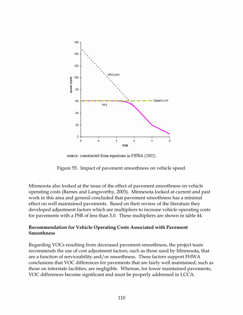
110
Figure 55. Impact of pavement smoothness on vehicle speed. Minnesota also looked at the issue of the effect of pavement smoothness on vehicle operating costs (Barnes and Langworthy, 2003). Minnesota looked at current and past work in this area and general concluded that pavement smoothness has a minimal effect on well maintained pavements. Based on their review of the literature they developed adjustment factors which are multipliers to increase vehicle operating costs for pavements with a PSR of less than 3.0. These multipliers are shown in table 44. Recommendation for Vehicle Operating Costs Associated with Pavement Smoothness Regarding VOCs resulting from decreased pavement smoothness, the project team recommends the use of cost adjustment factors, such as those used by Minnesota, that are a function of serviceability and/or smoothness. These factors support FHWA conclusions that VOC differences for pavements that are fairly well maintained, such as those on interstate facilities, are negligible. Whereas, for lower maintained pavements, VOC differences become significant and must be properly addressed in LCCA.
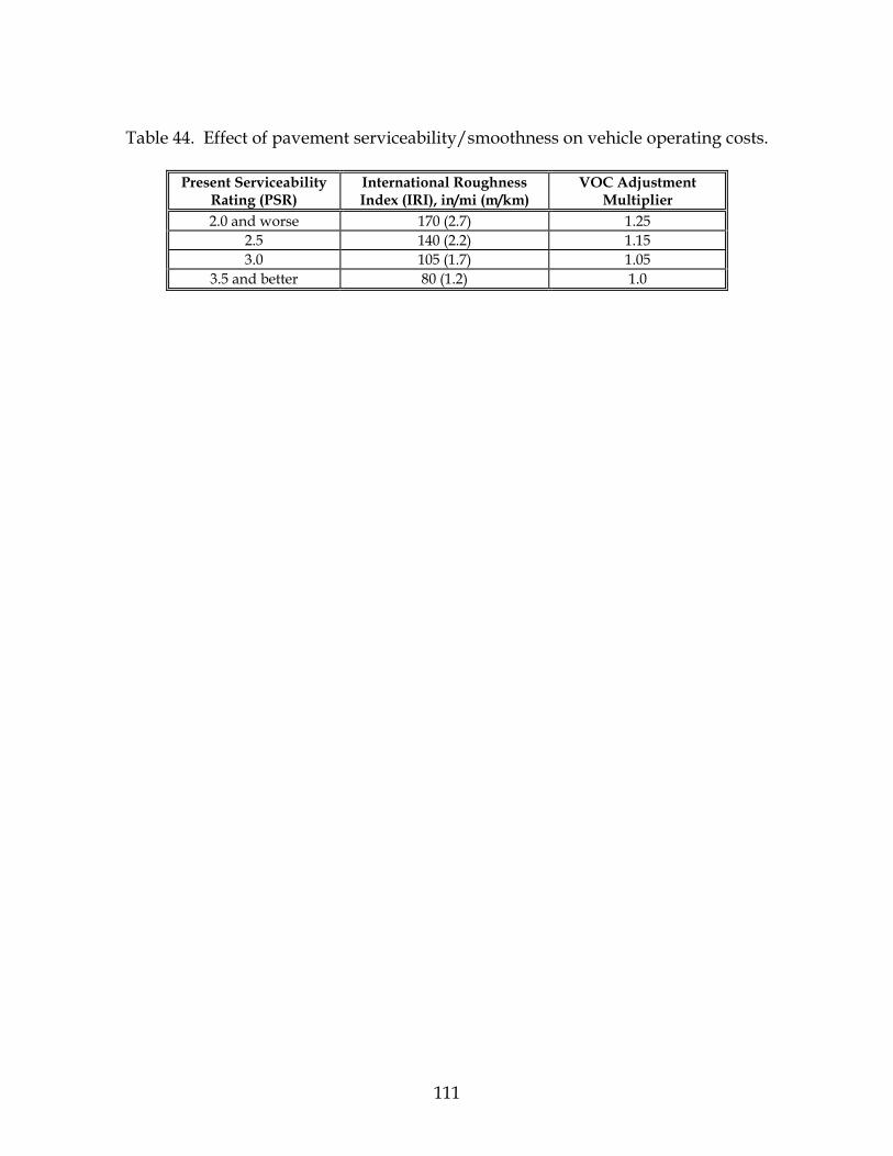
111
Table 44. Effect of pavement serviceability/smoothness on vehicle operating costs.
Present Serviceability
Rating (PSR) International Roughness Index (IRI), in/mi (m/km)
VOC Adjustment Multiplier
2.0 and worse 170 (2.7) 1.25 2.5 140 (2.2) 1.15 3.0 105 (1.7) 1.05
3.5 and better 80 (1.2) 1.0

112
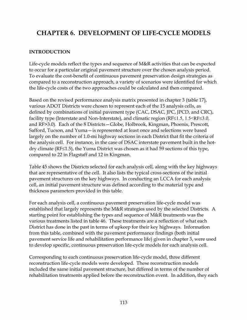
113
CHAPTER 6. DEVELOPMENT OF LIFE-CYCLE MODELS INTRODUCTION Life-cycle models reflect the types and sequence of M&R activities that can be expected to occur for a particular original pavement structure over the chosen analysis period. To evaluate the cost-benefit of continuous pavement preservation design strategies as compared to a reconstruction approach, a variety of scenarios were identified for which the life-cycle costs of the two approaches could be calculated and then compared. Based on the revised performance analysis matrix presented in chapter 3 (table 17), various ADOT Districts were chosen to represent each of the 15 analysis cells, as defined by combinations of initial pavement type (CAC, DSAC, JPC, JPCD, and CRC), facility type (Interstate and Non-Interstate), and climatic region (RF≤1.5, 1.5<RF≤3.0, and RF>3.0). Each of the 8 Districts—Globe, Holbrook, Kingman, Phoenix, Prescott, Safford, Tucson, and Yuma—is represented at least once and selections were based largely on the number of 1.0-mi highway sections in each District that fit the criteria of the analysis cell. For instance, in the case of DSAC interstate pavement built in the hot-dry climate (RF≤1.5), the Yuma District was chosen as it had 59 sections of this type, compared to 22 in Flagstaff and 12 in Kingman. Table 45 shows the Districts selected for each analysis cell, along with the key highways that are representative of the cell. It also lists the typical cross-sections of the initial pavement structures on the key highways. In conducting an LCCA for each analysis cell, an initial pavement structure was defined according to the material type and thickness parameters provided in this table. For each analysis cell, a continuous pavement preservation life-cycle model was established that largely represents the M&R strategies used by the selected Districts. A starting point for establishing the types and sequence of M&R treatments was the various treatments listed in table 46. These treatments are a reflection of what each District has done in the past in terms of upkeep for their key highways. Information from this table, combined with the pavement performance findings (both initial pavement service life and rehabilitation performance life) given in chapter 3, were used to develop specific, continuous preservation life-cycle models for each analysis cell. Corresponding to each continuous preservation life-cycle model, three different reconstruction life-cycle models were developed. These reconstruction models included the same initial pavement structure, but differed in terms of the number of rehabilitation treatments applied before the reconstruction event. In addition, they each

Table 45. Typical initial pavement structures corresponding to 15 revised analysis cells.
Climatic Zone Pavement Type Facility Type Hot-Dry (RF ≤ 1.5) Moderate (1.5 < RF ≤ 3.0) Cool-Wet (RF > 3.0)
Interstate
Yuma District (I-8, I-10) • 4.8” to 6.5” AC+FC • 4” AB • 5” to 20” SM (9” to 12” most typical)
Safford District (I-10) • 4” to 8.8” AC+FC (4” to 4.5” common for
‘60s design, 8.8” used on a few ‘70s sections)
• 6” AB or 4” BB (6” AB most common) • 12” to 21” SM (14” to 15” most typical)
CAC
Non-Interstate
Tucson District (SR 287, SR 347) • 4.5” AC+FC (SR 347) or 4.3” AC+SC (SR
287) • 8” to 10” AB
Holbrook District (US 180, SR 87, SR 264) • 3.3” to 4.3” AC+SC • 3” to 6” AB • 6” to 12” SM
Prescott District (SR 69 SR 260) • 4” to 8.3” AC or AC+FC • 6” to 18” AB (12” to 16” most common)
Interstate
Yuma District (I-10) • 9” to 13” AC+FC • 5” to 9” SM or 4” to 7” AB
or • 4.5” AC+FC • 2.5” to 5” BB • 3” to 5.5” AB
Kingman District (I-40) • 6” to 15” AC+FC (11.5” to 15” common
‘70s design, 9” to 11” common ‘80s/‘90s design)
• 6” to 28” AB (6” AB used in ‘70s/’80s, 24” to 28” used in ‘90s)
• 0” to 8” SM (5” to 8” used in ‘70s, 0” used in ‘90s)
Flagstaff District (I-17, I-40) • 8” to 11.5” AC or AC+FC (10” to 11.5”
used in ‘70s, 8” to 11” used in ‘80s) • 4” to 5” BB (‘80s designs only) • 6” to 8” AB (‘80s designs only) • 6” to 12” SM (‘70s designs only)
DSAC
Non-Interstate Kingman District (US 93, SR 68, SR 95) • 7” to 7.5” AC+FC • 4” to 6” AB
Safford District (US 19, SR 90, SR 92) • 4.3” to 9” AC or AC+SC • 6” to 14” AB
Globe District (US 180, SR 260) • 7.3” to 10.3” AC or AC+SC • 6” to 8” AB
JPC Interstate & Non-Interstate
Phoenix District (I-10, I-17, US 60, SR 101) • 9” to 16” PCC (9” common ‘60’s design
[I-10 and I-17], 11” to 13” common ‘90s/’00s design [US 60, SR 101])
• 4” AB or CB • 5” to 6” SM (SM used only in ‘60s)
Flagstaff District (I-17, I-40) • 8” to 10” PCC (8” common ‘70s design,
10” used a couple times in early ‘90s) • 4” to 6” CB • 4” to 6” SS or SM
JPCD Interstate & Non-Interstate
Phoenix Dist (I-10) • 10” to 13.5” PCC (9” to 10” common ‘80s
design, 12” to 13.5” common ’90s design) • 5” CL or 3” to 4” AC (LCB used in ‘80s,
AC used in ‘90s)
CRC Interstate & Non-Interstate
Phoenix Dist (I-17, SR 101) • 9” to 15” PCC (9” common ‘80s design
[SR 101], 13” common ’90 design [I-10], 15” common ’00s design [SR 101])
• 5” OA or 6” AB (OA used in ‘80s and ’90, AB used in ‘00s)
114

Table 46. Typical M&R treatments corresponding to 15 revised analysis cells.
Climatic Zone Pavement Type
Facility Type Hot-Dry (RF ≤ 1.5) Moderate (1.5 < RF ≤ 3.0) Cool-Wet (RF > 3.0)
Interstate
Yuma District (I-8, I-10) • 0 to 2 applications of FL or SR every 3 to 5
yrs (on initial structure) • RC+FC (2.5/3.0 to 5.0/5.5) • RC+FC (4.5/5.0) ⇒ RE+AC+FF (4.5/7.0) • RC+AC+FC (3.5/5.5 to 4.0/8.5) • RE+AC+FC (2.0/2.0) ⇒ RE+AR+FF
(2.0/2.5 to 2.0/4.5) • RE+AC+FF (3.0/5.5 to 4.5/6.5) • RC+RO+FC (4.0/6.0) • RC+RO+FC (4.0/5.0) ⇒ RC+AC+FF
(4.5/7.0)
Safford District (I-10) • 0 to 1 applications of FL every 8 yrs or 0 to
1 applications of SC or FC (0.5) every 5 to 14 yrs (on initial structure)
• LC+AC+FC (2.5) • LC+AC+FC (2.8 to 3.8) ⇒ RE+AC+FC
(3.0/3.0 to 4.0/8.0) • LC+AC+FC (2.8) ⇒ RC+AC+FC (3.0/5.5) ⇒ RE+AR+FR (2.5/2.5)
• LC+AC+FC (4.8) ⇒ FL ⇒ RE+AC+FC (2.8/2.5) ⇒ RE+AC+FC (4.0/6.5)
• LC+AS+FC (2.8) ⇒ FL ⇒ RC+AC+FC (4.5/6.5 to 6.0/9.5)
• RC+AC+FC (2.5/5.5) • RC+AC+FC (2.0/4.5 to 4.0/7.5) ⇒
RE+AC+FR (4.0/4.5 to 6.5/6.5) • RC+LC+AS+FC (4.0/6.7) ⇒ RE+AC+FC
(3.0/3.5)
CAC
Non-Interstate
Tucson District (SR 287, SR 347) • 0 to 1 applications of FC every 10 yrs (on
initial structure) • RE+AC (2.5/2.5) • RE+RO+AC+SC (2.0/3.8) • HS+FC (0.0/0.5) ⇒ RE+AC (2.5/2.5) ⇒
AC+FR (4.6)
Holbrook District (US 180, SR 87, SR 264) • 0 to 1 applications of FL every 4 yrs or 0 to
2 applications of SC every 3 to 5 yrs (on initial structure)
• AC+SC (2.3) • AC+SC (2.3) ⇒ SC ⇒ FR (0.8) • AC+SC (2.3) ⇒ FL+SC (0.3) ⇒ SC ⇒
AC+SC (1.8) • AC+SC+SC (3.0) ⇒ AC+SC+SC (3.0) • AC+SR (3.0)
Prescott District (SR 69 SR 260) • 0 to 1 applications of FL every 5 to 6 yrs
followed by 0 to 2 applications of SC every 5 to 15 yrs (on initial structure)
• AC+FC (2.0) ⇒ AC+FR (3.5) • AC+SC (1.8) ⇒ FR (0.5) • AC+SC (1.8) ⇒ SC+SC ⇒ FR (0.5) • RE+AR+FR (2.5/3.0)
115

Table 46. Typical M&R treatments corresponding to 15 revised analysis cells (continued).
Climatic Zone
Pavement Type
Facility Type Hot-Dry
(RF ≤ 1.5) Moderate
(1.5 < RF ≤ 3.0) Cool-Wet (RF > 3.0)
Interstate
Yuma District (I-10) • 0 to 2 applications of FL or SR every 3 to
5 years (initial structure) • RC+AC+FR (6.0/9.0) • RC+RO+FC (4.0/6.0) • RC+RO+FC (3.0/5.0) ⇒ RE+AC+FR
(4.5/7.0 to 9.5/12.0) • RE+AC+FR (6.0/6.5) • RE+AC+FC (2.5/2.5) ⇒ RE+AR+FR
(2.0/2.5)
Kingman District (I-40) • RE+FC (0.8/0.8) • RE+AC+FC (3.0/5.5 to 4.0/7.5) • RE+SuperPave+FR (5.5/5.5)
Flagstaff District (I-17, I-40) • RC+FC (2.0/2.5) ⇒ RE+AC+FR (5.0/5.5) • RE+FC (0.5) ⇒ RE+AC+FR (3.0/3.5) • RE+AR+FR (2.0/2.5)
DSAC
Non-Interstate
Kingman District (US 93, SR 68, SR 95) • None (no sections treated to date)
Safford District (US 19, SR 90, SR 92) • 0 to 1 applications of FL every 3 yrs or 0 to
1 applications of SC every 4 to 18 yrs (on initial structure)
• AC+SC (2.3) • AR+FR (2.2 to 2.5) • FR (0.5) • RE+AC+FL (1.0/2.0) ⇒ RE+AC+SC
(3.0/3.3) • SC+SC (0.5)
Globe District (US 180, SR 260) • 0 to 1 applications of SC every 5 to 6 yrs • AR (1.5)
JPC Interstate & Non-Interstate
Phoenix District (I-10, I-17, US 60, SR 101) • GR ⇒ FR (1.0) • FC+RM+FC (1.3) ⇒ RE+FR (1.0/1.0) • RE+FR (1.0)
* Based on I-10 & I-17 sections built in ‘60s
Flagstaff District (I-17, I-40) • AR (1.5) • AR+FR (2.5) ⇒ RE+AR+FR (2.0/2.5) • FR (1.0) ⇒ FR (0.5) • GR+FR (1.0) • KS+AC (4.0) ⇒ FR (1.0) • KS+AC (4.0) ⇒ RE+AC+FR (2.0/3.0) • KS+AC+AR+FR (5.5) • RM+AC+FC (2.8) ⇒ AC+AR+FR (5.5) • FL+LC+RM+FC+FL (1.8) ⇒ FR (1.0)
JPCD Interstate & Non-Interstate
Phoenix Dist (I-10) • None (no sections treated to date)
CRC Interstate & Non-Interstate
Phoenix Dist (I-17, SR 101) • None (no sections treated to date)
116
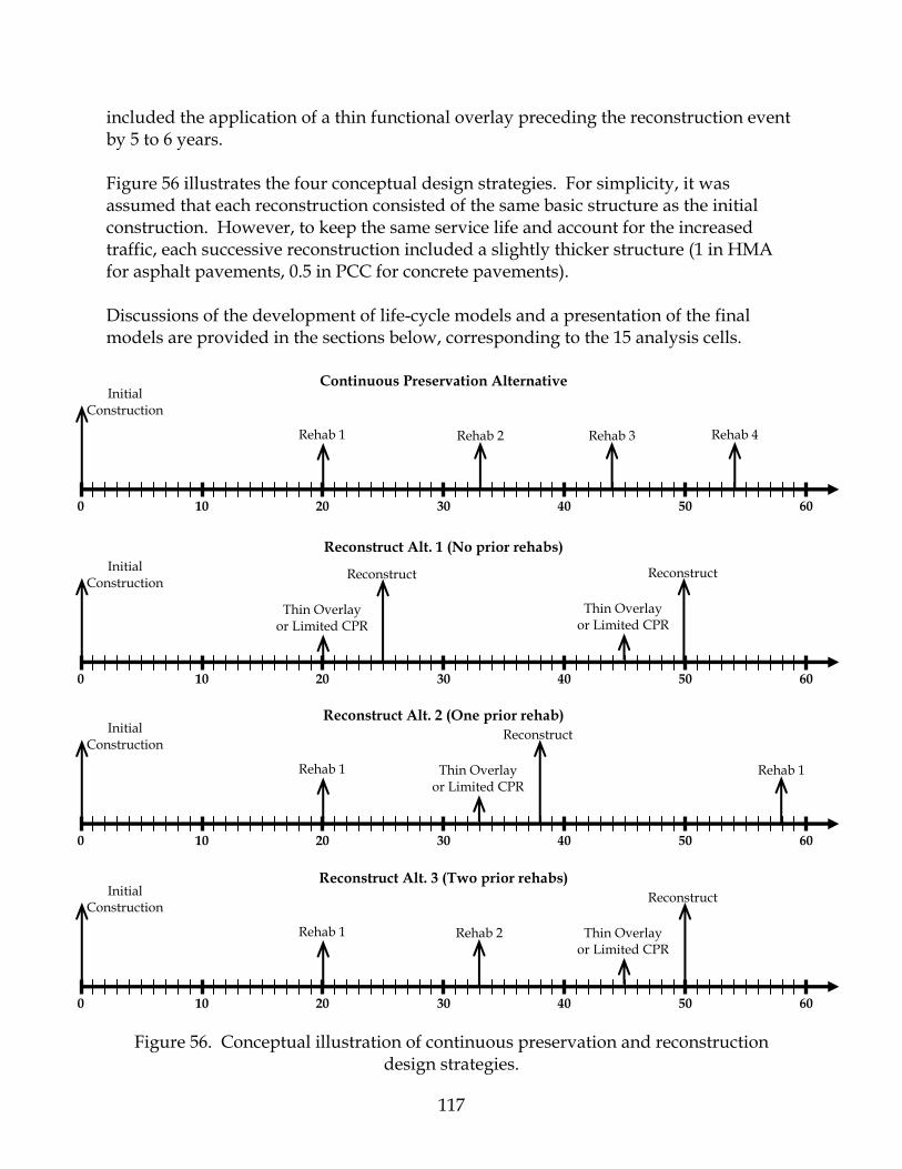
117
included the application of a thin functional overlay preceding the reconstruction event by 5 to 6 years. Figure 56 illustrates the four conceptual design strategies. For simplicity, it was assumed that each reconstruction consisted of the same basic structure as the initial construction. However, to keep the same service life and account for the increased traffic, each successive reconstruction included a slightly thicker structure (1 in HMA for asphalt pavements, 0.5 in PCC for concrete pavements). Discussions of the development of life-cycle models and a presentation of the final models are provided in the sections below, corresponding to the 15 analysis cells.
Figure 56. Conceptual illustration of continuous preservation and reconstruction design strategies.
0 10 20 30 40 50 60
Continuous Preservation Alternative Initial
Construction
Rehab 1 Rehab 2 Rehab 3 Rehab 4
0 10 20 30 40 50 60
Reconstruct Alt. 1 (No prior rehabs) Initial
Construction Reconstruct
Thin Overlay or Limited CPR
Reconstruct
Thin Overlay or Limited CPR
0 10 20 30 40 50 60
Reconstruct Alt. 2 (One prior rehab) Initial
Construction
Rehab 1 Rehab 1
Reconstruct
Thin Overlay or Limited CPR
0 10 20 30 40 50 60
Reconstruct Alt. 3 (Two prior rehabs) Initial
Construction
Rehab 1 Rehab 2
Reconstruct
Thin Overlay or Limited CPR
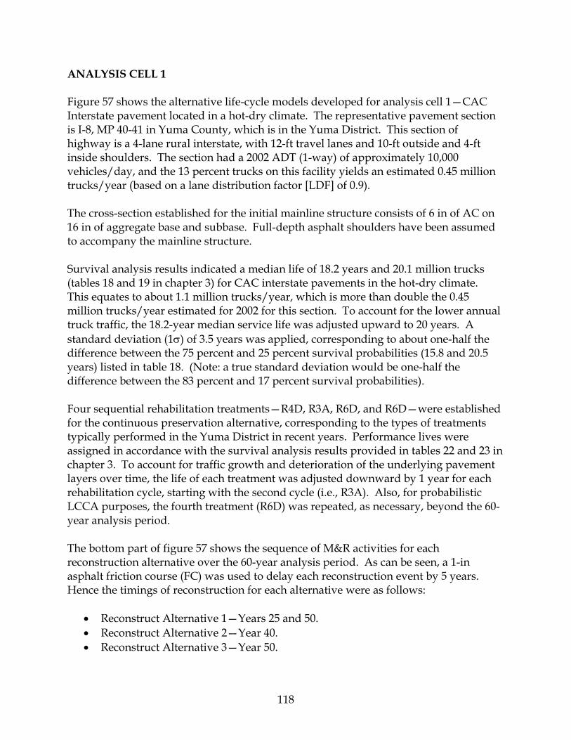
118
ANALYSIS CELL 1 Figure 57 shows the alternative life-cycle models developed for analysis cell 1—CAC Interstate pavement located in a hot-dry climate. The representative pavement section is I-8, MP 40-41 in Yuma County, which is in the Yuma District. This section of highway is a 4-lane rural interstate, with 12-ft travel lanes and 10-ft outside and 4-ft inside shoulders. The section had a 2002 ADT (1-way) of approximately 10,000 vehicles/day, and the 13 percent trucks on this facility yields an estimated 0.45 million trucks/year (based on a lane distribution factor [LDF] of 0.9). The cross-section established for the initial mainline structure consists of 6 in of AC on 16 in of aggregate base and subbase. Full-depth asphalt shoulders have been assumed to accompany the mainline structure. Survival analysis results indicated a median life of 18.2 years and 20.1 million trucks (tables 18 and 19 in chapter 3) for CAC interstate pavements in the hot-dry climate. This equates to about 1.1 million trucks/year, which is more than double the 0.45 million trucks/year estimated for 2002 for this section. To account for the lower annual truck traffic, the 18.2-year median service life was adjusted upward to 20 years. A standard deviation (1σ) of 3.5 years was applied, corresponding to about one-half the difference between the 75 percent and 25 percent survival probabilities (15.8 and 20.5 years) listed in table 18. (Note: a true standard deviation would be one-half the difference between the 83 percent and 17 percent survival probabilities). Four sequential rehabilitation treatments—R4D, R3A, R6D, and R6D—were established for the continuous preservation alternative, corresponding to the types of treatments typically performed in the Yuma District in recent years. Performance lives were assigned in accordance with the survival analysis results provided in tables 22 and 23 in chapter 3. To account for traffic growth and deterioration of the underlying pavement layers over time, the life of each treatment was adjusted downward by 1 year for each rehabilitation cycle, starting with the second cycle (i.e., R3A). Also, for probabilistic LCCA purposes, the fourth treatment (R6D) was repeated, as necessary, beyond the 60-year analysis period. The bottom part of figure 57 shows the sequence of M&R activities for each reconstruction alternative over the 60-year analysis period. As can be seen, a 1-in asphalt friction course (FC) was used to delay each reconstruction event by 5 years. Hence the timings of reconstruction for each alternative were as follows:
• Reconstruct Alternative 1—Years 25 and 50. • Reconstruct Alternative 2—Year 40. • Reconstruct Alternative 3—Year 50.

119
Activity Sequence for Reconstruction Alternatives Year Reconstruct Alt. #1 Reconstruct Alt. #2 Reconstruct Alt. #3
20 M2A (FC) (5.0 ± 0.0 yrs) 1” FC (1” AC)
R4D (RC+RO+FC) (15.0 ± 3.5 yrs) 0.5” FC (2” RO) 1.5” RO 3” RC Maint: FL every 5 yrs
R4D (RC+RO+FC) (15.0 ± 3.5 yrs) 0.5” FC (2” RO) 1.5” RO 3” RC Maint: FL every 5 yrs
25 CAC (Reconstruct) (20.0 ± 3.5 yrs) 0.5” FC (7” AC) 6.5” AC 4” AB (4” AB) 12” SM (12” SM) 23” RE (23” RE) Maint: FL every 5 yrs
35 M2A (FC) (5.0 ± 0.0 yrs) 1” FC (1” AC)
R3A (RE+AC+FC) (10.0 ± 2.0 yrs) 0.75” FC (0.25” SC) 1.5” AC 2.0” RE Maint: FL every 5 yrs
40 CAC (Reconstruct) (20.0 ± 3.5 yrs) 0.5” FC (8” AC) 7.5” AC 4” AB (4” AB) 12” SM (12” SM) 25” RE (25” RE) Maint: FL every 5 yrs
45 M2A (FC) (5.0 ± 0.0 yrs) 1” FC (1” AC)
M2A (FC) (5.0 ± 0.0 yrs) 1” FC (1” AC)
50 CAC (Reconstruct) (20.0 ± 3.5 yrs) 0.5” FC (8” AC) 7.5” AC 4” AB (4” AB) 12” SM (12” SM) 24” RE (24” RE) Maint: FL every 5 yrs
CAC (Reconstruct) (20.0 ± 3.5 yrs) 0.5” FC (8” AC) 7.5” AC 4” AB (4” AB) 12” SM (12” SM) 25.5” RE (25.5” RE) Maint: FL every 5 yrs
60 R4D (RC+RO+FC) (12.0 ± 2.5 yrs) 0.5” FC (2” RO) 1.5” RO 3” RC
Figure 57. Life-cycle models for analysis cell 1—CAC interstate pavement, hot-dry climate.
CAC (new) 0.5” FC (6” AC) 5.5” AC 4” AB (4” AB) 12” SM (12” SM)
Maint 0” FL
R4D (RC+RO+FC) 0.5” FC (2” RO) 1.5” RO 3” RC
Maint 0” FL
R3A (RE+AC+FC) 0.75” FC (0.25” SC) 1.5” AC 2.0” RE
Maint 0” FL
R6D (RC+AC+FC) 0.5” FC (2.5” AC) 6.5” AC 4.5” RC
20.0 + 3.5 yrs 15.0 + 3.5 yrs 10.0 + 2.0 yrs 12.0 + 3.0 yrs
Every 5 yrs Every 5 yrs Every 5 yrs Every 5 yrs
Maint 0” FL
0 10 20 30 40 50 60
Continuous Preservation Alternative
R6D (RC+AC+FC) 0.5” FC (2.5” AC) 6.5” AC 4.5” RC
12.0 + 2.75 yrs
Every 5 yrs
Maint 0” FL

120
ANALYSIS CELL 2 Figure 58 shows the alternative life-cycle models developed for analysis cell 2—CAC Interstate pavement located in a moderate climate. The representative pavement section is I-10, MP 385-386 in Cochise County, which is in the Safford District. This section of highway is a 4-lane rural interstate, with 12-ft travel lanes and 10-ft outside and 4-ft inside shoulders. The section had a 2002 ADT (1-way) of approximately 19,500 vehicles/day, and the 18 percent trucks on this facility yields an estimated 1.2 million trucks/year (LDF=0.9). The cross-section established for the initial mainline structure consists of 7 in of AC on 21 in of aggregate base and subbase. Full-depth asphalt shoulders have been assumed to accompany the mainline structure. Survival analysis results indicated a median life of 17.5 years and 15.2 million trucks (tables 18 and 19 in chapter 3) for CAC interstate pavements in the moderate climate. This equates to about 0.9 million trucks/year, which is somewhat less than the 1.2 million trucks/year estimated for 2002 for this section. To account for the higher annual truck traffic, the 17.5-year median service life was adjusted downward to 17 years. A standard deviation (1σ) of 3.0 years was applied, corresponding to about one-half the difference between the 75 percent and 25 percent survival probabilities (15.1 and 19.8 years) listed in table 18. Four sequential rehabilitation treatments—R3B, R4D, R3B, and R3B—were established for the continuous preservation alternative, corresponding to the types of treatments typically performed in the Safford District in recent years. Performance lives were assigned in accordance with the survival analysis results provided in tables 22 and 23 in chapter 3. To account for traffic growth and deterioration of the pavement layers over time, the life of each treatment was adjusted downward by 1 year for each rehabilitation cycle, starting with the second cycle (i.e., R4D). Also, for probabilistic LCCA purposes, the fourth treatment (R3B) was repeated, as necessary, beyond the 60-year analysis period. The bottom part of figure 58 shows the sequence of M&R activities for each reconstruction alternative over the 60-year analysis period. As can be seen, a 1-in asphalt rubber friction course (FR) was used to delay each reconstruction event by 5 years. Hence the timings of reconstruction for each alternative were as follows:
• Reconstruct Alternative 1—Years 22 and 44. • Reconstruct Alternative 2—Year 34. • Reconstruct Alternative 3—Year 47.
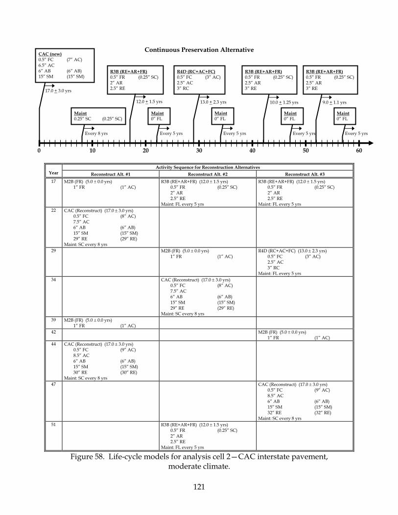
121
Activity Sequence for Reconstruction Alternatives Year Reconstruct Alt. #1 Reconstruct Alt. #2 Reconstruct Alt. #3
17 M2B (FR) (5.0 ± 0.0 yrs) 1” FR (1” AC)
R3B (RE+AR+FR) (12.0 ± 1.5 yrs) 0.5” FR (0.25” SC) 2” AR 2.5” RE Maint: FL every 5 yrs
R3B (RE+AR+FR) (12.0 ± 1.5 yrs) 0.5” FR (0.25” SC) 2” AR 2.5” RE Maint: FL every 5 yrs
22 CAC (Reconstruct) (17.0 ± 3.0 yrs) 0.5” FC (8” AC) 7.5” AC 6” AB (6” AB) 15” SM (15” SM) 29” RE (29” RE) Maint: SC every 8 yrs
29 M2B (FR) (5.0 ± 0.0 yrs) 1” FR (1” AC)
R4D (RC+AC+FC) (13.0 ± 2.3 yrs) 0.5” FC (3” AC) 2.5” AC 3” RC Maint: FL every 5 yrs
34 CAC (Reconstruct) (17.0 ± 3.0 yrs) 0.5” FC (8” AC) 7.5” AC 6” AB (6” AB) 15” SM (15” SM) 29” RE (29” RE) Maint: SC every 8 yrs
39 M2B (FR) (5.0 ± 0.0 yrs) 1” FR (1” AC)
42 M2B (FR) (5.0 ± 0.0 yrs) 1” FR (1” AC)
44 CAC (Reconstruct) (17.0 ± 3.0 yrs) 0.5” FC (9” AC) 8.5” AC 6” AB (6” AB) 15” SM (15” SM) 30” RE (30” RE) Maint: SC every 8 yrs
47 CAC (Reconstruct) (17.0 ± 3.0 yrs) 0.5” FC (9” AC) 8.5” AC 6” AB (6” AB) 15” SM (15” SM) 32” RE (32” RE) Maint: SC every 8 yrs
51 R3B (RE+AR+FR) (12.0 ± 1.5 yrs) 0.5” FR (0.25” SC) 2” AR 2.5” RE Maint: FL every 5 yrs
Figure 58. Life-cycle models for analysis cell 2—CAC interstate pavement, moderate climate.
CAC (new) 0.5” FC (7” AC) 6.5” AC 6” AB (6” AB) 15” SM (15” SM)
Maint 0.25” SC (0.25” SC)
R3B (RE+AR+FR) 0.5” FR (0.25” SC) 2” AR 2.5” RE
Maint 0” FL
R4D (RC+AC+FC) 0.5” FC (3” AC) 2.5” AC 3” RC
Maint 0” FL
R3B (RE+AR+FR) 0.5” FR (0.25” SC) 2.5” AR 3” RE 17.0 + 3.0 yrs
12.0 + 1.5 yrs 13.0 + 2.3 yrs 10.0 + 1.25 yrs
Every 8 yrs Every 5 yrs Every 5 yrs Every 5 yrs
Maint 0” FL
0 10 20 30 40 50 60
Continuous Preservation Alternative
R3B (RE+AR+FR) 0.5” FR (0.25” SC) 2.5” AR 3” RE
9.0 + 1.1 yrs
Every 5 yrs
Maint 0” FL
122
ANALYSIS CELL 3 Figure 59 shows the alternative life-cycle models developed for analysis cell 3—CAC Non-Interstate pavement located in a hot-dry climate. The representative pavement section is SR 287, MP 115-116 in Pinal County, which is in the Tucson District. This section of highway is a 2-lane rural highway, with 12-ft travel lanes and 5-ft shoulders. The section had a 2002 ADT (1-way) of approximately 13,000 vehicles/day, and the 5 percent trucks on this facility yields an estimated 0.25 million trucks/year (LDF=1). The cross-section established for the initial mainline structure consists of 5.25 in of AC on 10 in of aggregate base. Full-depth asphalt shoulders have been assumed to accompany the mainline structure. Survival analysis results indicated a median life of 21.6 years and 5.8 million trucks (tables 18 and 19 in chapter 3) for CAC Non-Interstate pavements in the hot-dry climate. This equates to about 0.27 million trucks/year, which is slightly higher than the 0.25 million trucks/year estimated for 2002 for this section. For purposes of LCCA, the 21.6-year median service life was rounded upward to 22 years. A standard deviation (1σ) of 5.0 years was applied, corresponding to about one-half the difference between the 75 percent and 25 percent survival probabilities (16.7 and 26.5 years) listed in table 18. Three sequential rehabilitation treatments—all R3A—were established for the continuous preservation alternative, corresponding to the types of treatments typically performed in the Tucson District in recent years. Performance lives were assigned in accordance with the survival analysis results provided in tables 22 and 23 in chapter 3. To account for traffic growth and deterioration of the pavement layers over time, the life of each treatment was adjusted downward by 1 year for each rehabilitation cycle, starting with the second cycle. Also, for probabilistic LCCA purposes, the R3A treatment was repeated, as necessary, beyond the 60-year analysis period. The bottom part of figure 59 shows the sequence of M&R activities for each reconstruction alternative over the 60-year analysis period. As can be seen, a 1-in asphalt friction course (FC) was used to delay each reconstruction event by 6 years. Hence the timings of reconstruction for each alternative were as follows:
• Reconstruct Alternative 1—Years 28 and 57. • Reconstruct Alternative 2—Year 45. • Reconstruct Alternative 3—Year 60.

123
Activity Sequence for Reconstruction Alternatives Year Reconstruct Alt. #1 Reconstruct Alt. #2 Reconstruct Alt. #3
22 M2A (FC) (6.0 ± 0.0 yrs) 1” FC (1” AC)
R3A (RE+AC+SC) (17.0 ± 5.0 yrs) 0.25” SC (0.25” SC) 3” AC (1” AC) 2” RE Maint: FL every 10 yrs
R3A (RE+AC+SC) (17.0 ± 5.0 yrs) 0.25” SC (0.25” SC) 3” AC (1” AC) 2” RE Maint: FL every 10 yrs
28 CAC (Reconstruct) (22.0 ± 5.0 yrs) 0.25” SC (0.25” SC) 6” AC (6” AC) 10” AB (10” AB) 16.5” RE (16.5” RE) Maint: FL every 10 yrs
39 M2A (FC) (6.0 ± 0.0 yrs) 1” FC (1” AC)
R3A (RE+AC+SC) (16.0 ± 4.5 yrs) 0.25” SC (0.25” SC) 3” AC (1” AC) 2” RE Maint: FL every 10 yrs
45 CAC (Reconstruct) (22.0 ± 5.0 yrs) 0.25” SC (0.25” SC) 7” AC (7” AC) 10” AB (10” AB) 17.5” RE (17.5” RE) Maint: FL every 10 yrs
50 M2A (FC) (6.0 ± 0.0 yrs) 1” FC (1” AC)
54 M2A (FC) (6.0 ± 0.0 yrs) 1” FC (1” AC)
57 CAC (Reconstruct) (22.0 ± 5.0 yrs) 0.25” SC (0.25” SC) 7” AC (7” AC) 10” AB (10” AB) 17.5” RE (17.5” RE) Maint: FL every 10 yrs
60 CAC (Reconstruct) (22.0 ± 5.0 yrs) 0.25” SC (0.25” SC) 7” AC (7” AC) 10” AB (10” AB) 19” RE (19” RE) Maint: FL every 10 yrs
Figure 59. Life-cycle models for analysis cell 3—CAC non-interstate pavement, hot-dry climate.
CAC (new) 0.25” SC (0.25” SC) 5” AC (5” AC) 10” AB (10” AB)
Maint 0” FL
R3A (RE+AC+SC) 0.25” SC (0.25” SC) 3” AC (1” AC) 2” RE
Maint 0” FL
R3A (RE+AC+SC) 0.25” SC (0.25” SC) 3” AC (1” AC) 2” RE
Maint 0” FL
22.0 + 5.0 yrs
17.0 + 5.0 yrs 16.0 + 4.5 yrs
Every 10 yrs Every 10 yrs Every 10 yrs
0 10 20 30 40 50 60
Continuous Preservation Alternative
Maint 0” FL
R3A (RE+AC+SC) 0.25” SC (0.25” SC) 3” AC (1” AC) 2” RE
15.0 + 4.0 yrs
Every 10 yrs
124
ANALYSIS CELL 4 Figure 60 shows the alternative life-cycle models developed for analysis cell 4—CAC Non-Interstate pavement located in a moderate climate. The representative pavement section is SR 264, MP 475-476 in Apache County, which is in the Holbrook District. This section of highway is a 4-lane rural highway, with 12-ft travel lanes and 4-ft shoulders. The section had a 2002 ADT (1-way) of approximately 5,500 vehicles/day, and the 6 percent trucks on this facility yields an estimated 0.11 million trucks/year (LDF=0.9). The cross-section established for the initial mainline structure consists of 4.25 in of AC on 14 in of aggregate base and subbase. Full-depth asphalt shoulders have been assumed to accompany the mainline structure. Survival analysis results indicated a median life of 27.8 years and 6.5 million trucks (tables 18 and 19 in chapter 3) for CAC Non-Interstate pavements in the moderate climate. This equates to about 0.23 million trucks/year, which is higher than the 0.11 million trucks/year estimated for 2002 for this section. For purposes of LCCA, the 27.8-year median service life was rounded upward to 28 years. A standard deviation (1σ) of 6.75 years was applied, corresponding to about one-half the difference between the 75 percent and 25 percent survival probabilities (21.2 and 34.4 years) listed in table 18. Two sequential rehabilitation treatments—both R1A—were established for the continuous preservation alternative, corresponding to the types of treatments typically performed in the Holbrook District in recent years. Performance lives were assigned in accordance with the survival analysis results provided in tables 22 and 23 in chapter 3. To account for traffic growth and deterioration of the pavement layers over time, the life of each treatment was adjusted downward by 2 years for each rehabilitation cycle, starting with the second cycle. Also, for probabilistic LCCA purposes, the R1A treatment was repeated, as necessary, beyond the 60-year analysis period. The bottom part of figure 60 shows the sequence of M&R activities for each reconstruction alternative over the 60-year analysis period. As can be seen, a 1-in asphalt friction course (FC) was used to delay each reconstruction event by 6 years. Hence, the timings of reconstruction for each alternative were as follows:
• Reconstruct Alternative 1—Year 33. • Reconstruct Alternative 2—Year 57. • Reconstruct Alternative 3—None. For the 60-year analysis period, the activity
sequence for this alternative is the same as that for continuous preservation. However, the first event after the 60-year analysis period is different for the two alternatives. For the continuous preservation alternative, the next event is the R1A rehabilitation treatment, whereas for Alternative 3, the next event is M2A.

125
Activity Sequence for Reconstruction Alternatives Year Reconstruct Alt. #1 Reconstruct Alt. #2 Reconstruct Alt. #3
27 M2A (FC) (6.0 ± 0.0 yrs) 1” FC (1” AC)
R1A (AC+DC) (24.0 ± 7.0 yrs) 0.5” DC (0.5” DC) 2.5” AC (2.5” AC) Maint: FL every 5 yrs
R1A (AC+DC) (24.0 ± 7.0 yrs) 0.5” DC (0.5” DC) 2.5” AC (2.5” AC) Maint: FL every 5 yrs
33 CAC (Reconstruct) (27.0 ± 6.5 yrs) 0.25” SC (0.25” SC) 5” AC (5” AC) 4” AB (4” AB) 10” SM (10” SM) 16.5” RE (16.5” RE) Maint: SC every 5 yrs
51 M2A (FC) (6.0 ± 0.0 yrs) 1” FC (1” AC)
R1A (AC+DC) (22.0 ± 6.0 yrs) 0.5” DC (0.5” DC) 2.5” AC (2.5” AC) Maint: FL every 5 yrs
57 CAC (Reconstruct) (27.0 ± 6.5 yrs) 0.25” SC (0.25” SC) 6” AC (6” AC) 4” AB (4” AB) 10” SM (10” SM) 21.5” RE (21.5” RE) Maint: SC every 5 yrs
60 M2A (FC) (6.0 ± 0.0 yrs) 1” FC (1” AC)
Figure 60. Life-cycle models for analysis cell 4—CAC non-interstate pavement, moderate climate.
CAC (new) 0.25” SC (0.25” SC) 4” AC (4” AC) 4” AB (4” AB) 10” SM (10” SM)
Maint 0.25” SC (0.25” SC)
R1A (AC+DC) 0.5” DC (0.5” DC) 2.5” AC (2.5” AC)
R1A (AC+DC) 0.5” DC (0.5” DC) 2.5” AC (2.5” AC)
Maint 0” FL
27.0 + 6.5 yrs
24.0 + 7.0 yrs 22.0 + 6.0 yrs
Every 5 yrs Every 5 yrs
0 10 20 30 40 50 60
Continuous Preservation Alternative
Maint 0” FL
Every 5 yrs

126
ANALYSIS CELL 5 Figure 61 shows the alternative life-cycle models developed for analysis cell 5—CAC Non-Interstate pavement located in a cool-wet climate. The representative pavement section is SR 260, MP 290-291 in Gila County, which is in the Prescott District. This section of highway is a 4-lane rural highway, with 12-ft travel lanes and 4-ft inside and 10-ft outside shoulders. The section had a 2002 ADT (1-way) of approximately 5,000 vehicles/day, and the 10 percent trucks on this facility yields an estimated 0.17 million trucks/year (LDF=0.9). The cross-section established for the initial mainline structure consists of 4.5 in of AC on 16 in of aggregate base. Full-depth asphalt shoulders have been assumed to accompany the mainline structure. Survival analysis results indicated a median life of 15.1 years and 5.3 million trucks (tables 18 and 19 in chapter 3) for CAC Non-Interstate pavements in the cool-wet climate. This equates to about 0.35 million trucks/year, which is higher than the 0.17 million trucks/year estimated for 2002 for this section. For purposes of LCCA, the 15.1-year median service life was rounded upward to 18 years. A standard deviation (1σ) of 5.5 years was applied, corresponding to about one-half the difference between the 75 percent and 25 percent survival probabilities (9.8 and 20.8 years) listed in table 18. Three sequential rehabilitation treatments—all R1A—were established for the continuous preservation alternative, corresponding to the types of treatments typically performed in the Prescott District in recent years. Performance lives were assigned in accordance with the survival analysis results provided in tables 22 and 23 in chapter 3. To account for traffic growth and deterioration of the pavement layers over time, the life of each treatment was adjusted downward by 2 years for each rehabilitation cycle, starting with the second cycle. Also, for probabilistic LCCA purposes, the R1A treatment was repeated, as necessary, beyond the 60-year analysis period. The bottom part of figure 61 shows the sequence of M&R activities for each reconstruction alternative over the 60-year analysis period. As can be seen, a 1-in asphalt friction course (FC) was used to delay each reconstruction event by 6 years. Hence, the timings of reconstruction for each alternative were as follows:
• Reconstruct Alternative 1—Years 24 and 48. • Reconstruct Alternative 2—Year 45. • Reconstruct Alternative 3—None.

127
Activity Sequence for Reconstruction Alternatives Year Reconstruct Alt. #1 Reconstruct Alt. #2 Reconstruct Alt. #3
18 M2A (FC) (6.0 ± 0.0 yrs) 1” FC (1” AC)
R1A (AC+FC) (21.0 ± 6.0 yrs) 0.5” FC (3” AC) 2.5” AC Maint: FL every 7 yrs
R1A (AC+FC) (21.0 ± 6.0 yrs) 0.5” FC (3” AC) 2.5” AC Maint: FL every 7 yrs
24 CAC (Reconstruct) (18.0 ± 5.0 yrs) 5.5” AC (5.5” AC) 16” AB (16” AB) 22” RE (22” RE) Maint: SC every 7 yrs
39 M2A (FC) (6.0 ± 0.0 yrs) 1” FC (1” AC)
R1A (AC+FC) (19.0 ± 5.0 yrs) 0.5” FC (3” AC) 2.5” AC Maint: FL every 7 yrs
42 M2A (FC) (6.0 ± 0.0 yrs) 1” FC (1” AC)
45 CAC (Reconstruct) (18.0 ± 5.0 yrs) 6.5” AC (6.5” AC) 16” AB (16” AB) 25” RE (25” RE) Maint: SC every 7 yrs
48 CAC (Reconstruct) (18.0 ± 5.0 yrs) 6.5” AC (6.5” AC) 16” AB (16” AB) 23” RE (23” RE) Maint: SC every 7 yrs
58 M2A (FC) (6.0 ± 0.0 yrs) 1” FC (1” AC)
Figure 61. Life-cycle models for analysis cell 5—CAC non-interstate pavement, cool-wet climate.
CAC (new) 4.5” AC (4.5” AC) 16” AB (16” AB)
Maint 0.25” SC (0.25” SC)
R1A (AC+FC) 0.5” FC (3” AC) 2.5” AC
Maint 0” FL
R1A (AC+FC) 0.5” FC (3” AC) 2.5” AC
Maint 0” FL
R1A (AC+FC) 0.5” FC (3” AC) 2.5” AC 18.0 + 5.0 yrs
21.0 + 6.0 yrs 19.0 + 5.0 yrs 17.0 + 4.0 yrs
Every 7 yrs Every 7 yrs Every 7 yrs
0 10 20 30 40 50 60
Continuous Preservation Alternative

128
ANALYSIS CELL 6 Figure 62 shows the alternative life-cycle models developed for analysis cell 6—DSAC Interstate pavement located in a hot-dry climate. The representative pavement section is I-10, MP 100-101 in Maricopa County, which is in the Yuma District. This section of highway is a 4-lane rural interstate, with 12-ft travel lanes and 4-ft inside and 10-ft outside shoulders. The section had a 2002 ADT (1-way) of approximately 22,000 vehicles/day, and the 18 percent trucks on this facility yields an estimated 1.3 million trucks/year (LDF=0.9). The cross-section established for the initial mainline structure consists of 10.5 in of asphalt (5.5 in AC, 5 in BB) on 6 in of aggregate base. Full-depth asphalt shoulders have been assumed to accompany the mainline structure. Survival analysis results indicated a median life of 16.9 years and 19.4 million trucks (tables 18 and 19 in chapter 3) for DSAC Interstate pavements in the hot-dry climate. This equates to about 1.15 million trucks/year, which is a little less than the 1.3 million trucks/year estimated for 2002 for this section. For purposes of LCCA, the 16.9-year median service life was rounded downward to 17 years. A standard deviation (1σ) of 2.5 years was applied, corresponding to about one-half the difference between the 75 percent and 25 percent survival probabilities (14.7 and 19.2 years) listed in table 18. Four sequential rehabilitation treatments—R3B, R3B, R6D, and R6B—were established for the continuous preservation alternative, corresponding to the types of treatments typically performed in the Yuma District in recent years. Performance lives were assigned in accordance with the survival analysis results provided in tables 22 and 23 in chapter 3. To account for traffic growth and deterioration of the pavement layers over time, the life of each treatment was adjusted downward by 1 year for each rehabilitation cycle, starting with the second cycle. Also, for probabilistic LCCA purposes, the fourth treatment (R6B) was repeated, as necessary, beyond the 60-year analysis period. The bottom part of figure 62 shows the sequence of M&R activities for each reconstruction alternative over the 60-year analysis period. As can be seen, a 1-in asphalt friction course (FC) was used to delay each reconstruction event by 5 years. Hence, the timings of reconstruction for each alternative were as follows:
• Reconstruct Alternative 1—Years 22 and 39. • Reconstruct Alternative 2—Years 36 and 58. • Reconstruct Alternative 3—Year 49.
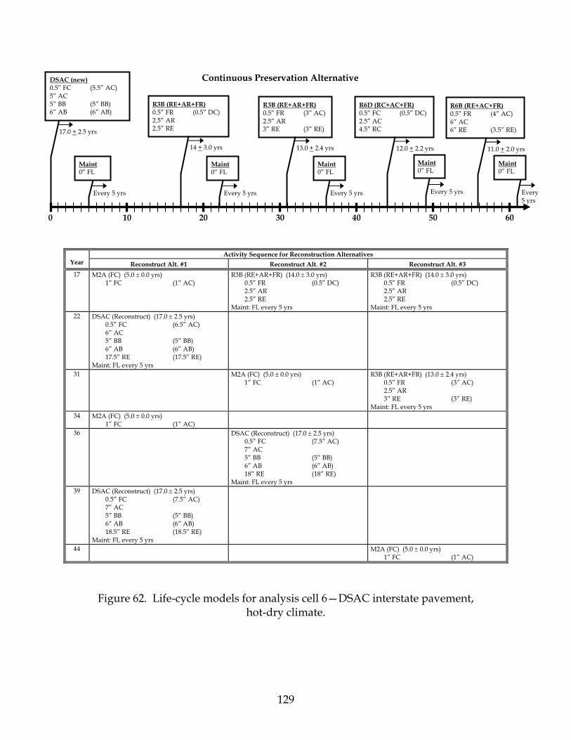
129
Activity Sequence for Reconstruction Alternatives Year Reconstruct Alt. #1 Reconstruct Alt. #2 Reconstruct Alt. #3
17 M2A (FC) (5.0 ± 0.0 yrs) 1” FC (1” AC)
R3B (RE+AR+FR) (14.0 ± 3.0 yrs) 0.5” FR (0.5” DC) 2.5” AR 2.5” RE Maint: FL every 5 yrs
R3B (RE+AR+FR) (14.0 ± 3.0 yrs) 0.5” FR (0.5” DC) 2.5” AR 2.5” RE Maint: FL every 5 yrs
22 DSAC (Reconstruct) (17.0 ± 2.5 yrs) 0.5” FC (6.5” AC) 6” AC 5” BB (5” BB) 6” AB (6” AB) 17.5” RE (17.5” RE) Maint: FL every 5 yrs
31 M2A (FC) (5.0 ± 0.0 yrs) 1” FC (1” AC)
R3B (RE+AR+FR) (13.0 ± 2.4 yrs) 0.5” FR (3” AC) 2.5” AR 3” RE (3” RE) Maint: FL every 5 yrs
34 M2A (FC) (5.0 ± 0.0 yrs) 1” FC (1” AC)
36 DSAC (Reconstruct) (17.0 ± 2.5 yrs) 0.5” FC (7.5” AC) 7” AC 5” BB (5” BB) 6” AB (6” AB) 18” RE (18” RE) Maint: FL every 5 yrs
39 DSAC (Reconstruct) (17.0 ± 2.5 yrs) 0.5” FC (7.5” AC) 7” AC 5” BB (5” BB) 6” AB (6” AB) 18.5” RE (18.5” RE) Maint: FL every 5 yrs
44 M2A (FC) (5.0 ± 0.0 yrs) 1” FC (1” AC)
Figure 62. Life-cycle models for analysis cell 6—DSAC interstate pavement, hot-dry climate.
DSAC (new) 0.5” FC (5.5” AC) 5” AC 5” BB (5” BB) 6” AB (6” AB)
Maint 0” FL
R3B (RE+AR+FR) 0.5” FR (0.5” DC) 2.5” AR 2.5” RE
Maint 0” FL
R3B (RE+AR+FR) 0.5” FR (3” AC) 2.5” AR 3” RE (3” RE)
Maint 0” FL
R6D (RC+AC+FR) 0.5” FC (0.5” DC) 2.5” AC 4.5” RC 17.0 + 2.5 yrs
14 + 3.0 yrs 13.0 + 2.4 yrs 12.0 + 2.2 yrs
Every 5 yrs Every 5 yrs Every 5 yrs
0 10 20 30 40 50 60
Continuous Preservation Alternative
Maint 0” FL
Every 5 yrs
R6B (RE+AC+FR) 0.5” FR (4” AC) 6” AC 6” RE (3.5” RE)
11.0 + 2.0 yrs
Maint 0” FL
Every 5 yrs

130
Activity Sequence for Reconstruction Alternatives
Year Reconstruct Alt. #1 Reconstruct Alt. #2 Reconstruct Alt. #3 49 DSAC (Reconstruct) (17.0 ± 2.5 yrs)
0.5” FC (7.5” AC) 8” AC 5” BB (5” BB) 6” AB (6” AB) 18” RE (18” RE) Maint: FL every 5 yrs
53 M2A (FC) (5.0 ± 0.0 yrs) 1” FC (1” AC)
56 M2A (FC) (5.0 ± 0.0 yrs) 1” FC (1” AC)
58 DSAC (Reconstruct) (17.0 ± 2.5 yrs) 0.5” FC (7.5” AC) 8” AC 5” BB (5” BB) 6” AB (6” AB) 18.5” RE (18.5” RE) Maint: FL every 5 yrs
Figure 62. Life-cycle models for analysis cell 6—DSAC interstate pavement, hot-dry climate (continued).

131
ANALYSIS CELL 7 Figure 63 shows the alternative life-cycle models developed for analysis cell 7—DSAC Interstate pavement located in a moderate climate. The representative pavement section is I-40, MP 120-121 in Yapapai County, which is in the Kingman District. This section of highway is a 4-lane rural interstate, with 12-ft travel lanes and 4-ft inside and 10-ft outside shoulders. The section had a 2002 ADT (1-way) of approximately 17,000 vehicles/day, and the 24 percent trucks on this facility yields an estimated 1.3 million trucks/year (LDF=0.9). The cross-section established for the initial mainline structure consists of 10 in of AC on 12 in of aggregate base. Full-depth asphalt shoulders have been assumed to accompany the mainline structure. Survival analysis results indicated a median life of 18.4 years and 16.2 million trucks (tables 18 and 19 in chapter 3) for DSAC Interstate pavements in the hot-dry climate. This equates to about 0.88 million trucks/year, which is less than the 1.3 million trucks/year estimated for 2002 for this section. For purposes of LCCA, the 18.4-year median service life was adjusted downward to 17 years. A standard deviation (1σ) of 3.75 years was applied, corresponding to about one-half the difference between the 75 percent and 25 percent survival probabilities (14.8 and 21.9 years) listed in table 18. Three sequential rehabilitation treatments—all R4A—were established for the continuous preservation alternative, corresponding to the types of treatments typically performed in the Kingman District in recent years. Performance lives were assigned in accordance with the survival analysis results provided in tables 22 and 23 in chapter 3. To account for traffic growth and deterioration of the pavement layers over time, the life of each treatment was adjusted downward by 2 years for each rehabilitation cycle, starting with the second cycle. Also, for probabilistic LCCA purposes, the R4A treatment was repeated, as necessary, beyond the 60-year analysis period. The bottom part of figure 63 shows the sequence of M&R activities for each reconstruction alternative over the 60-year analysis period. As can be seen, a 0.75-in mill-and-replacement with asphalt friction course (FC) was used to delay each reconstruction event by 5 years. Hence, the timings of reconstruction for each alternative were as follows:
• Reconstruct Alternative 1—Years 22 and 44. • Reconstruct Alternative 2—Year 40. • Reconstruct Alternative 3—Year 56.
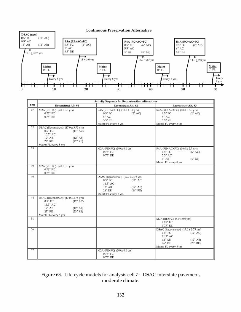
132
Activity Sequence for Reconstruction Alternatives Year Reconstruct Alt. #1 Reconstruct Alt. #2 Reconstruct Alt. #3
17 M2A (RE+FC) (5.0 ± 0.0 yrs) 0.75” FC 0.75” RE
R4A (RE+AC+FC) (18.0 ± 3.0 yrs) 0.5” FC (2” AC) 5” AC 3.5” RE Maint: FL every 8 yrs
R4A (RE+AC+FC) (18.0 ± 3.0 yrs) 0.5” FC (2” AC) 5” AC 3.5” RE Maint: FL every 8 yrs
22 DSAC (Reconstruct) (17.0 ± 3.75 yrs) 0.5” FC (11” AC) 10.5” AC 12” AB (12” AB) 22” RE (22” RE) Maint: FL every 8 yrs
35 M2A (RE+FC) (5.0 ± 0.0 yrs) 0.75” FC 0.75” RE
R4A (RE+AC+FC) (16.0 ± 2.7 yrs) 0.5” FC (6” AC) 5.5” AC 4” RE (4” RE) Maint: FL every 8 yrs
39 M2A (RE+FC) (5.0 ± 0.0 yrs) 0.75” FC 0.75” RE
40 DSAC (Reconstruct) (17.0 ± 3.75 yrs) 0.5” FC (12” AC) 11.5” AC 12” AB (12” AB) 24” RE (24” RE) Maint: FL every 8 yrs
44 DSAC (Reconstruct) (17.0 ± 3.75 yrs) 0.5” FC (12” AC) 11.5” AC 12” AB (12” AB) 23” RE (23” RE) Maint: FL every 8 yrs
51 M2A (RE+FC) (5.0 ± 0.0 yrs) 0.75” FC 0.75” RE
56 DSAC (Reconstruct) (17.0 ± 3.75 yrs) 0.5” FC (12” AC) 11.5” AC 12” AB (12” AB) 26” RE (26” RE) Maint: FL every 8 yrs
57 M2A (RE+FC) (5.0 ± 0.0 yrs) 0.75” FC 0.75” RE
Figure 63. Life-cycle models for analysis cell 7—DSAC interstate pavement, moderate climate.
DSAC (new) 0.5” FC (10” AC) 9.5” AC 12” AB (12” AB)
Maint 0” FL
R4A (RE+AC+FC) 0.5” FC (2” AC) 5” AC 3.5” RE
Maint 0” FL
R4A (RC+AC+FC) 0.5” FC (6” AC) 5.5” AC 4” RE (4” RE)
Maint 0” FL
17.0 + 3.75 yrs
18 + 3.0 yrs 16.0 + 2.7 yrs 14.0 + 2.3 yrs
Every 8 yrs Every 8 yrs Every 8 yrs
0 10 20 30 40 50 60
Continuous Preservation Alternative
Maint 0” FL
Every 8 yrs
R4A (RC+AC+FC) 0.5” FC (2” AC) 6” AC 4.5” RE
133
ANALYSIS CELL 8 Figure 64 shows the alternative life-cycle models developed for analysis cell 8—DSAC Interstate pavement located in a cool-wet climate. The representative pavement section is I-17, MP 311-312 in Coconino County, which is in the Flagstaff District. This section of highway is a 4-lane rural interstate, with 12-ft travel lanes and 4-ft inside and 8-ft outside shoulders. The section had a 2002 ADT (1-way) of approximately 23,000 vehicles/day, and the 15 percent trucks on this facility yields an estimated 1.1 million trucks/year (LDF=0.9). The cross-section established for the initial mainline structure consists of 10.5 in of AC on 8 in of aggregate base. Full-depth asphalt shoulders have been assumed to accompany the mainline structure. Survival analysis results indicated a median life of 13.2 years and 13.1 million trucks (tables 18 and 19 in chapter 3) for DSAC Interstate pavements in the cool-wet climate. This equates to about 1 million trucks/year, slightly lower than the 1.1 million trucks/year estimated for 2002 for this section. Because the 13.2-year median service life was derived from a limited number of observations (15 total pavement sections) and because mechanistic analysis indicated a service life greater than 20 years for this design, the service life was adjusted upward to 15 years. A standard deviation (1σ) of 3.5 years was applied, corresponding to about one-half the difference between the 75 percent and 25 percent survival probabilities (10.0 and 16.4 years) listed in table 18. Four sequential rehabilitation treatments—R3D, R3B, R6B, and R6B—were established for the continuous preservation alternative, corresponding to the types of treatments typically performed in the Flagstaff District in recent years. Performance lives were assigned in accordance with the survival analysis results provided in tables 22 and 23 in chapter 3. To account for traffic growth and deterioration of the pavement layers over time, the life of each treatment was adjusted downward by 1 year for each rehabilitation cycle, starting with the second cycle. Also, for probabilistic LCCA purposes, the fourth treatment (R6B) was repeated, as necessary, beyond the 60-year analysis period. The bottom part of figure 64 shows the sequence of M&R activities for each reconstruction alternative over the 60-year analysis period. As can be seen, a 0.75-in mill-and-replacement with asphalt friction course (FC) was used to delay each reconstruction event by 5 years. Hence, the timings of reconstruction for each alternative were as follows:
• Reconstruct Alternative 1—Years 20, 40, and 60. • Reconstruct Alternative 2—Year 32. • Reconstruct Alternative 3—Year 44.

134
Activity Sequence for Reconstruction Alternatives Year Reconstruct Alt. #1 Reconstruct Alt. #2 Reconstruct Alt. #3
15 M2A (RE+FC) (5.0 ± 0.0 yrs) 0.75” FC 0.75” RE
R3D (RC+FC) (12.0 ± 2.5 yrs) 0.5” FC (0.5” DC) 2.5” RC Maint: FL every 5 yrs
R3D (RC+FC) (12.0 ± 2.5 yrs) 0.5” FC (0.5” DC) 2.5” RC Maint: FL every 5 yrs
20 DSAC (Reconstruct) (15.0 ± 3.5 yrs) 0.5” FC (11.5” AC) 11” AC 8” AB (8” AB) 18.5” RE (18.5” RE) Maint: FL every 5 yrs
27 M2A (RE+FC) (5.0 ± 0.0 yrs) 0.75” FC 0.75” RE
R3B (RE+AC+FR) (12.0 ± 2.5 yrs) 0.5” FR (3.5” AC) 3” AC 3” RE (3” RE) Maint: FL every 5 yrs
32 DSAC (Reconstruct) (15.0 ± 3.5 yrs) 0.5” FC (11.5” AC) 11” AC 8” AB (8” AB) 19” RE (19” RE) Maint: FL every 5 yrs
35 M2A (RE+FC) (5.0 ± 0.0 yrs) 0.75” FC 0.75” RE
39 M2A (RE+FC) (5.0 ± 0.0 yrs) 0.75” FC 0.75” RE
40 DSAC (Reconstruct) (15.0 ± 3.5 yrs) 0.5” FC (12.5” AC) 12” AC 8” AB (8” AB) 19.5” RE (19.5” RE) Maint: FL every 5 yrs
44 DSAC (Reconstruct) (15.0 ± 3.5 yrs) 0.5” FC (12.5” AC) 12” AC 8” AB (8” AB) 19.5” RE (19.5” RE) Maint: FL every 5 yrs
47 R3D (RC+FC) (11.0 ± 2.25 yrs) 0.5” FC (0.5” DC) 2.5” RC Maint: FL every 5 yrs
Figure 64. Life-cycle models for analysis cell 8—DSAC interstate pavement, cool-wet climate.
DSAC (new) 0.5” FC (10.5” AC) 10” AC 8” AB (8” AB)
Maint 0” FL
R3D (RC+FC) 0.5” FC (0.5” DC) 2.5” RC
Maint 0” FL
R3B (RE+AC+FR) 0.5” FR (3.5” AC) 3” AC 3” RE (3” RE)
Maint 0” FL
15.0 + 3.5 yrs
12.0 + 2.5 yrs 12.0 + 2.5 yrs 13.0 + 3.0 yrs
Every 5 yrs Every 5 yrs Every 5 yrs
0 10 20 30 40 50 60
Continuous Preservation Alternative
Maint 0” FL
Every 5 yrs
R6B (RE+AC+FR) 0.5” FR (0.5” DC) 5” AC 5” RE
12.0 + 2.8 yrs
Maint 0” FL
Every 5 yrs
R6B (RE+AC+FR) 0.5” FR (0.5” DC) 5” AC 5” RE

135
Activity Sequence for Reconstruction Alternatives Year Reconstruct Alt. #1 Reconstruct Alt. #2 Reconstruct Alt. #3
55 M2A (RE+FC) (5.0 ± 0.0 yrs) 0.75” FC 0.75” RE
58 M2A (RE+FC) (5.0 ± 0.0 yrs) 0.75” FC 0.75” RE
59 R3D (RC+FC) (10.0 ± 2.0 yrs) 0.5” FC (0.5” DC) 2.5” RC Maint: FL every 5 yrs
60 DSAC (Reconstruct) (15.0 ± 3.5 yrs) 0.5” FC (13.5” AC) 13” AC 8” AB (8” AB) 19.5” RE (19.5” RE) Maint: FL every 5 yrs
Figure 64. Life-cycle models for analysis cell 8—DSAC interstate pavement, cool-wet climate (continued).
136
ANALYSIS CELL 9 Figure 65 shows the alternative life-cycle models developed for analysis cell 9—DSAC Non-Interstate pavement located in a hot-dry climate. The representative pavement section is US 93, MP 40-41 in Mohave County, which is in the Kingman District. This section of highway is a 4-lane rural interstate, with 12-ft travel lanes and 4-ft inside and 10-ft outside shoulders. The section had a 2002 ADT (1-way) of approximately 9,000 vehicles/day, and the 11 percent trucks on this facility yields an estimated 0.35 million trucks/year (LDF=0.9). The cross-section established for the initial mainline structure consists of 7.5 in of AC on 4 in of aggregate base. Partial-depth asphalt shoulders have been assumed to accompany the mainline structure. Survival analysis results indicated a median life of 23.9 years and 12.4 million trucks (tables 18 and 19 in chapter 3) for DSAC Non-Interstate pavements in the hot-dry climate. This equates to about 0.5 million trucks/year, a little higher than the 0.35 million trucks/year estimated for 2002 for this section. For purposes of LCCA, the 23.9-year median service life was adjusted upward to 25 years. A standard deviation (1σ) of 5.5 years was applied, corresponding to about one-half the difference between the 75 percent and 25 percent survival probabilities (18.7 and 29.1 years) listed in table 18. Two sequential rehabilitation treatments—R1A and R4A—were established for the continuous preservation alternative, corresponding to the types of treatments typically performed in the Kingman District in recent years. Performance lives were assigned in accordance with the survival analysis results provided in tables 22 and 23 in chapter 3. To account for traffic growth and deterioration of the pavement layers over time, the life of each treatment was adjusted downward by 2 years for each rehabilitation cycle, starting with the second cycle. Also, for probabilistic LCCA purposes, the second treatment (R4A) was repeated, as necessary, beyond the 60-year analysis period. The bottom part of figure 65 shows the sequence of M&R activities for each reconstruction alternative over the 60-year analysis period. As can be seen, a 1-in asphalt friction course (FC) was used to delay each reconstruction event by 6 years. Hence, the timings of reconstruction for each alternative were as follows:
• Reconstruct Alternative 1—Year 31. • Reconstruct Alternative 2—Year 56. • Reconstruct Alternative 3—None. For the 60-year analysis period, the activity
sequence for this alternative is the same as for continuous preservation. However, the first event after the 60-year analysis period is different for the two alternatives. For the continuous preservation alternative, the next event is the R4A rehabilitation treatment, whereas for Alternative 3, the next event is M2A

137
Activity Sequence for Reconstruction Alternatives Year Reconstruct Alt. #1 Reconstruct Alt. #2 Reconstruct Alt. #3
25 M2A (FC) (6.0 ± 0.0 yrs) 1” FC (1” AC)
R1A (AC+FC) (25.0 ± 6.0 yrs) 0.5” FC (3” AC) 2.5” AC Maint: SC every 7 yrs
R1A (AC+FC) (25.0 ± 6.0 yrs) 0.5” FC (3” AC) 2.5” AC Maint: SC every 7 yrs
31 DSAC (Reconstruct) (25.0 ± 5.5 yrs) 0.5” FC (4.5” AC) 8” AC (8” AB) 4” AB 13.5” RE (13.5” RE) Maint: SC every 7 yrs
50 M2A (FC) (6.0 ± 0.0 yrs) 1” FC (1” AC)
R4A (RE+AC+FC) (19.0 ± 4.1 yrs) 0.5” FC (5.5” AC) 5” AC 4” RE (4” RE)
56 M2A (FC) (6.0 ± 0.0 yrs) 1” FC (1” AC)
DSAC (Reconstruct) (25.0 ± 5.5 yrs) 0.5” FC (5.5” AC) 9” AC (8” AB) 4” AB 16.5” RE (16.5” RE) Maint: SC every 7 yrs
Figure 65. Life-cycle models for analysis cell 9—DSAC non-interstate pavement, hot-dry climate.
DSAC (new) 0.5” FC (3.5” AC) 7” AC (8” AB) 4” AB
Maint 0.25” SC (0.25” SC)
R1A (AC+FC) 0.5” FC (3” AC) 2.5” AC
R4A (RE+AC+FC) 0.5” FC (5.5” AC) 5” AC 4” RE (4” RE) 25.0 + 5.5 yrs
25.0 + 6.0 yrs 19.0 + 4.1 yrs
Every 7 yrs Every 7 yrs
0 10 20 30 40 50 60
Continuous Preservation Alternative
Every 7 yrs
Maint 0.25” SC (0.25” SC)
Maint 0.25” SC (0.25” SC)

138
ANALYSIS CELL 10 Figure 66 shows the alternative life-cycle models developed for analysis cell 10—DSAC Non-Interstate pavement located in a moderate climate. The representative pavement section is SR 90, MP 320-321 in Cochise County, which is in the Safford District. This section of highway is a 2-lane rural highway, with 12-ft travel lanes and 4-ft shoulders. The section had a 2002 ADT (1-way) of approximately 14,000 vehicles/day, and the 10 percent trucks on this facility yields an estimated 0.5 million trucks/year (LDF=1.0). The cross-section established for the initial mainline structure consists of 8.5 in of AC on 6 in of aggregate base. Partial-depth asphalt shoulders have been assumed to accompany the mainline structure. Survival analysis results indicated a median life of 26.8 years and 6.4 million trucks (tables 18 and 19 in chapter 3) for DSAC Non-Interstate pavements in the moderate climate. This equates to about 0.25 million trucks/year, which is one-half the 0.5 million trucks/year estimated for 2002 for this section. For purposes of LCCA, the 26.8-year median service life was adjusted downward to 23 years. A standard deviation (1σ) of 6.5 years was applied, corresponding to about one-half the difference between the 75 percent and 25 percent survival probabilities (19.9 and 33.7 years) listed in table 18. Two sequential rehabilitation treatments—R1A and R3A—were established for the continuous preservation alternative, corresponding to the types of treatments typically performed in the Safford District in recent years. Performance lives were assigned in accordance with the survival analysis results provided in tables 22 and 23 in chapter 3. To account for traffic growth and deterioration of the pavement layers over time, the life of each treatment was adjusted downward by 2 years for each rehabilitation cycle, starting with the second cycle. Also, for probabilistic LCCA purposes, the second treatment (R3A) was repeated, as necessary, beyond the 60-year analysis period. The bottom part of figure 66 shows the sequence of M&R activities for each reconstruction alternative over the 60-year analysis period. As can be seen, a 1-in asphalt friction course (FC) was used to delay each reconstruction event by 6 years. Hence, the timings of reconstruction for each alternative were as follows:
• Reconstruct Alternative 1—Years 29 and 58. • Reconstruct Alternative 2—Year 53. • Reconstruct Alternative 3—None. For the 60-year analysis period, the activity
sequence for this alternative is the same as for continuous preservation. However, the first event after the 60-year analysis period is different for the two alternatives. For the continuous preservation alternative, the next event is the R3A rehabilitation treatment, whereas for Alternative 3, the next event is M2A.

139
Activity Sequence for Reconstruction Alternatives Year Reconstruct Alt. #1 Reconstruct Alt. #2 Reconstruct Alt. #3
23 M2A (FC) (6.0 ± 0.0 yrs) 1” FC (1” AC)
R1A (AC+SC) (24.0 ± 6.5 yrs) 0.25” SC (0.25” SC) 3” AC (3” AC) Maint: SC every 5 yrs
R1A (AC+SC) (24.0 ± 6.5 yrs) 0.25” SC (0.25” SC) 3” AC (3” AC) Maint: SC every 5 yrs
29 DSAC (Reconstruct) (23.0 ± 6.5 yrs) 9.5” AC (4.5” AC) 6.5” AB (11.5” AB) 17” RE (17” RE) Maint: SC every 5 yrs
47 M2A (FC) (6.0 ± 0.0 yrs) 1” FC (1” AC)
R3A (RE+AC+SC) (14.0 ± 2.5 yrs) 0.25” SC (0.25” SC) 3” AC (3” AC) 3” RE (3” RE)
52 M2A (FC) (6.0 ± 0.0 yrs) 1” FC (1” AC)
53 DSAC (Reconstruct) (23.0 ± 6.5 yrs) 10.5” AC (5.5” AC) 6.5” AB (11.5” AB) 20.5” RE (20.5” RE) Maint: SC every 5 yrs
58 DSAC (Reconstruct) (23.0 ± 6.5 yrs) 10.5” AC (5.5” AC) 6.5” AB (11.5” AB) 18” RE (18” RE) Maint: SC every 5 yrs
Figure 66. Life-cycle models for analysis cell 10—DSAC non-interstate pavement, moderate climate.
DSAC (new) 8.5” AC (3.5” AC) 6.5” AB (11.5” AB)
Maint 0.25” SC (0.25” SC)
R1A (AC+SC) 0.25” SC (0.25” SC) 3” AC (3” AC)
R3A (RE+AC+SC) 0.25” SC (0.25” SC) 3” AC (3” AC) 3” RE (3” RE) 23.0 + 6.5 yrs
24.0 + 6.5 yrs 14.0 + 2.5 yrs
Every 5 yrs Every 5 yrs
0 10 20 30 40 50 60
Continuous Preservation Alternative
Every 5 yrs
Maint 0.25” SC (0.25” SC)
Maint 0.25” SC (0.25” SC)

140
ANALYSIS CELL 11 Figure 67 shows the alternative life-cycle models developed for analysis cell 11—DSAC Non-Interstate pavement located in a cool-wet climate. The representative pavement section is US 180, MP 405-406 in Apache County, which is in the Globe District. This section of highway is a 2-lane rural highway, with 12-ft travel lanes and 5-ft shoulders. The section had a 2002 ADT (1-way) of approximately 1,400 vehicles/day, and the 7 percent trucks on this facility yields an estimated 0.04 million trucks/year (LDF=1.0). The cross-section established for the initial mainline structure consists of 9.25 in of AC on 6 in of aggregate base. Partial-depth asphalt shoulders have been assumed to accompany the mainline structure. Survival analysis results indicated a median life of 23.2 years and 3.7 million trucks (tables 18 and 19 in chapter 3) for DSAC Non-Interstate pavements in the cool-wet climate. This equates to about 0.16 million trucks/year, which is triple the 0.04 million trucks/year estimated for 2002 for this section. For purposes of LCCA, the 23.2-year median service life was adjusted upward to 26 years. A standard deviation (1σ) of 6.5 years was applied, corresponding to about one-half the difference between the 75 percent and 25 percent survival probabilities (16.8 and 29.5 years) listed in table 18. Three sequential rehabilitation treatments—R1B, R3B, and R1B—were established for the continuous preservation alternative, corresponding to the types of treatments typically performed in the Globe District in recent years. Performance lives were assigned in accordance with the survival analysis results provided in tables 22 and 23 in chapter 3. To account for traffic growth and deterioration of the pavement layers over time, the life of each treatment was adjusted downward by 1 year for each rehabilitation cycle, starting with the second cycle. Also, for probabilistic LCCA purposes, the third treatment (R1B) was repeated, as necessary, beyond the 60-year analysis period. The bottom part of figure 67 shows the sequence of M&R activities for each reconstruction alternative over the 60-year analysis period. As can be seen, a 1-in asphalt rubber (AR) overlay was used to delay each reconstruction event by 6 years. Hence, the timings of reconstruction for each alternative were as follows:
• Reconstruct Alternative 1—Year 32. • Reconstruct Alternative 2—Year 45. • Reconstruct Alternative 3—Year 58.

141
Activity Sequence for Reconstruction Alternatives Year Reconstruct Alt. #1 Reconstruct Alt. #2 Reconstruct Alt. #3
26 M2B (AR) (6.0 ± 0.0 yrs) 1” AR (1” AR)
R1B (AR) (13.0 ± 3.5 yrs) 3” AR (3” AR) Maint: SC every 7 yrs
R1B (AR) (13.0 ± 3.5 yrs) 3” AR (3” AR) Maint: SC every 7 yrs
32 DSAC (Reconstruct) (26.0 ± 6.5 yrs) 0.25” SC (0.25” SC) 11” AC (4.5” AC) 6” AB (12.5” AB) 18” RE (18” RE) Maint: SC every 7 yrs
39 M2B (AR) (6.0 ± 0.0 yrs) 1” AR (1” AR)
R3B (RE+AR) (13.0 ± 3.0 yrs) 3.5” AR (3.5” AR) 3.5” RE (3.5” RE) Maint: SC every 7 yrs
45 DSAC (Reconstruct) (26.0 ± 6.5 yrs) 0.25” SC (0.25” SC) 11” AC (4.5” AC) 6” AB (12.5” AB) 21” RE (21” RE) Maint: SC every 7 yrs
52 M2B (AR) (6.0 ± 0.0 yrs) 1” AR (1” AR)
58 M2B (AR) (6.0 ± 0.0 yrs) 1” AR (1” AR)
DSAC (Reconstruct) (26.0 ± 6.5 yrs) 0.25” SC (0.25” SC) 11” AC (4.5” AC) 6” AB (12.5” AB) 22” RE (22” RE) Maint: SC every 7 yrs
Figure 67. Life-cycle models for analysis cell 11—DSAC non-interstate pavement, cool-wet climate.
DSAC (new) 0.25” SC (0.25” SC) 10” AC (3.5’ AC) 6” AB (12.5” AB)
Maint 0.25” SC (0.25” SC)
R1B (AR) 3” AR (3” AR)
R3B (RE+AR) 3.5” AR (3.5” AR) 3.5” RE (3.5” RE) 26.0 + 6.5 yrs
13.0 + 3.5 yrs 13.0 + 3.0 yrs
Every 7 yrs Every 7 yrs
0 10 20 30 40 50 60
Continuous Preservation Alternative
Every 7 yrs
Maint 0.25” SC (0.25” SC)
Maint 0.25” SC (0.25” SC)
R1B (AR) 3” AR (3” AR)
11.0 + 3.0 yrs
Every 7 yrs
Maint 0.25” SC (0.25” SC)
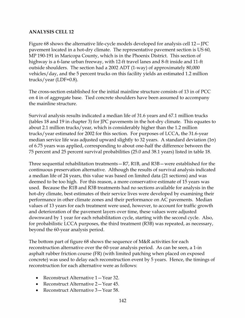
142
ANALYSIS CELL 12 Figure 68 shows the alternative life-cycle models developed for analysis cell 12—JPC pavement located in a hot-dry climate. The representative pavement section is US 60, MP 190-191 in Maricopa County, which is in the Phoenix District. This section of highway is a 6-lane urban freeway, with 12-ft travel lanes and 8-ft inside and 11-ft outside shoulders. The section had a 2002 ADT (1-way) of approximately 80,000 vehicles/day, and the 5 percent trucks on this facility yields an estimated 1.2 million trucks/year (LDF=0.8). The cross-section established for the initial mainline structure consists of 13 in of PCC on 4 in of aggregate base. Tied concrete shoulders have been assumed to accompany the mainline structure. Survival analysis results indicated a median life of 31.6 years and 67.1 million trucks (tables 18 and 19 in chapter 3) for JPC pavements in the hot-dry climate. This equates to about 2.1 million trucks/year, which is considerably higher than the 1.2 million trucks/year estimated for 2002 for this section. For purposes of LCCA, the 31.6-year median service life was adjusted upward slightly to 32 years. A standard deviation (1σ) of 6.75 years was applied, corresponding to about one-half the difference between the 75 percent and 25 percent survival probabilities (25.0 and 38.1 years) listed in table 18. Three sequential rehabilitation treatments—R7, R1B, and R3B—were established for the continuous preservation alternative. Although the results of survival analysis indicated a median life of 24 years, this value was based on limited data (21 sections) and was deemed to be too high. For this reason, a more conservative estimate of 15 years was used. Because the R1B and R3B treatments had no sections available for analysis in the hot-dry climate, best estimates of their service lives were developed by examining their performance in other climate zones and their performance on AC pavements. Median values of 13 years for each treatment were used, however, to account for traffic growth and deterioration of the pavement layers over time, these values were adjusted downward by 1 year for each rehabilitation cycle, starting with the second cycle. Also, for probabilistic LCCA purposes, the third treatment (R3B) was repeated, as necessary, beyond the 60-year analysis period. The bottom part of figure 68 shows the sequence of M&R activities for each reconstruction alternative over the 60-year analysis period. As can be seen, a 1-in asphalt rubber friction course (FR) (with limited patching when placed on exposed concrete) was used to delay each reconstruction event by 5 years. Hence, the timings of reconstruction for each alternative were as follows:
• Reconstruct Alternative 1—Year 32. • Reconstruct Alternative 2—Year 45. • Reconstruct Alternative 3—Year 58.

143
Activity Sequence for Reconstruction Alternatives Year Reconstruct Alt. #1 Reconstruct Alt. #2 Reconstruct Alt. #3
32 M2B (FR) (5.0 ± 0.0 yrs) 1” FR (1” AC) 1% PDR (AC) (0.2% PDR (AC)) 1% FDR (0.2% FDR)
R7 (GR) (15.0 ± 3.5 yrs) 0.5% PDR (0.1% PDR) 5% FDR (1% FDR) 100% GR T/L Jt Seal (T/L Jt Seal)
R7 (GR) (16.0 ± 3.5 yrs) 0.5% PDR (0.1% PDR) 5% FDR (1% FDR) 100% GR T/L Jt Seal (T/L Jt Seal)
37 JPC (Reconstruct) (32.0 ± 6.75 yrs) 13.5” PC (13.5” PC) 4” AB (4” AB) 18” RE (18” RE)
47 M2B (FR) (5.0 ± 0.0 yrs) 1” FR (1” AC)
R1B (AR+FR) (12.0 ± 2.75 yrs) 0.5” FR (2.5” AC) 2” AR 0.5% PDR (0.1% PDR) 5% FDR (2% FDR)
52 JPC (Reconstruct) (32.0 ± 6.75 yrs) 14” PC (14” PC) 4” AB (4” AB) 18” RE (18” RE)
59 M2B (FR) (5.0 ± 0.0 yrs) 1” FR (1” AC)
Figure 68. Life-cycle models for analysis cell 12—JPC pavement, hot-dry climate.
JPC (new) 13” PC (13” PC) 4” AB (4” AB)
Maint 0.5% FDR T/L Jt Seal (T/L Jt Seal)
R7 (GR) 0.5% PDR (0.1% PDR) 5% FDR (1% FDR) 100% GR T/L Jt Seal (T/L Jt Seal)
R1B (AR+FR) 0.5” FR (2.5” AC) 2” AR 0.5% PDR (0.1% PDR) 5% FDR (2% FDR) 32.0 + 6.75 yrs
15.0 + 3.5 yrs 12.0 + 2.75 yrs
Every 15 yrs
0 10 20 30 40 50 60
Continuous Preservation Alternative
Every 7 yrs
Maint 0” FL
R3B (RE+AR+FR) 0.5” FR 2” AR 2.5” RE
11.0 + 2.5 yrs
Every 7 yrs
Maint 0” FL
Maint 0.5% FDR
Every 10 yrs

144
ANALYSIS CELL 13 Figure 69 shows the alternative life-cycle models developed for analysis cell 13—JPC pavement located in a cool-wet climate. The representative pavement section is I-17, MP 330-331 in Coconino County, which is in the Flagstaff District. This section of highway is a 4-lane rural interstate, with 12-ft travel lanes and 4-ft inside and 10-ft outside shoulders. The section had a 2002 ADT (1-way) of approximately 25,000 vehicles/day, and the 15 percent trucks on this facility yields an estimated 1.2 million trucks/year (LDF=0.9). The cross-section established for the initial mainline structure consists of 11 in of PCC on 6 in of aggregate base. Tied concrete shoulders have been assumed to accompany the mainline structure. Survival analysis results indicated a median life of 19.6 years and 10.2 million trucks (tables 18 and 19 in chapter 3) for mostly 8-in JPC pavements in the cool-wet climate. Although based on a limited number of pavement sections (27), this equates to about 0.6 million trucks/year, which is about one-half the 1.2 million trucks/year estimated for 2002 for this section. Because this heavier truck traffic would be more than offset by the thicker slab (11 in instead of 8 in), the 19.6-year median service life was adjusted upward to 25 years. A standard deviation (1σ) of 5.5 years was applied as a more reasonable estimate than what would be given by the difference in the 75 percent and 25 percent survival probabilities (19.2 and 19.9 years) listed in table 18. Three sequential rehabilitation treatments—R7, R10B, and R3B—were established for the continuous preservation alternative. Because no performance estimates for these treatments were available from the survival analysis, best estimates were developed by examining the raw performance data and the performance estimates of similar applications. To account for traffic growth and deterioration of the pavement layers over time, the best estimate values were adjusted downward by 1 year for each rehabilitation cycle, starting with the second cycle. Also, for probabilistic LCCA purposes, the third treatment (R3B) was repeated, as necessary, beyond the 60-year analysis period. The bottom part of figure 69 shows the sequence of M&R activities for each reconstruction alternative over the 60-year analysis period. As can be seen, a 1-in asphalt rubber friction course (FR) (with limited patching when placed on exposed concrete) was used to delay each reconstruction event by 5 years. Hence, the timings of reconstruction for each alternative were as follows:
• Reconstruct Alternative 1—Year 32. • Reconstruct Alternative 2—Year 45. • Reconstruct Alternative 3—Year 58.

145
Activity Sequence for Reconstruction Alternatives Year Reconstruct Alt. #1 Reconstruct Alt. #2 Reconstruct Alt. #3
25 M2B (FR) (5.0 ± 0.0 yrs) 1” FR (1” AC) 1% PDR (AC) (0.2% PDR (AC)) 1% FDR (0.2% FDR)
R7 (GR) (13.0 ± 3.0 yrs) 0.5% PDR (0.1% PDR) 5% FDR (1% FDR) 100% GR T/L Jt Seal (T/L Jt Seal)
R7 (GR) (13.0 ± 3.0 yrs) 0.5% PDR (0.1% PDR) 5% FDR (1% FDR) 100% GR T/L Jt Seal (T/L Jt Seal)
30 JPC (Reconstruct) (25.0 ± 5.5 yrs) 11.5” PC (11.5” PC) 6” AB (6” AB) 18” RE (18” RE)
38 M2B (FR) (5.0 ± 0.0 yrs) 1” FR (1” AC) 1% PDR (AC) (0.2% PDR (AC)) 1% FDR (0.2% FDR)
R10B (GR+FR) (13.0 ± 2.75 yrs) 1” FR (1” AC) 2.5% PDR (AC) (1% PDR (AC)) 5% FDR (1% FDR) 100% GR
43 JPC (Reconstruct) (25.0 ± 5.5 yrs) 11.5” PC (11.5” PC) 6” AB (6” AB) 18” RE (18” RE)
51 M2B (RE+FR) (5.0 ± 0.0 yrs) 1” FR 1” RE
55 M2B (FR) (5.0 ± 0.0 yrs) 1” FR (1” AC) 1% PDR (AC) (0.2% PDR (AC)) 1% FDR (0.2% FDR)
56 JPC (Reconstruct) (25.0 ± 5.5 yrs) 12” PC (12” PC) 6” AB (6” AB) 18” RE (18” RE)
60 JPC (Reconstruct) (25.0 ± 5.5 yrs) 12” PC (12” PC) 6” AB (6” AB) 18.5” RE (18.5” RE)
Figure 69. Life-cycle models for analysis cell 13—JPC pavement, cool-wet climate.
JPC (new) 11” PC (11” PC) 6” AB (6” AB)
Maint 0.5% FDR T/L Jt Seal (T/L Jt Seal)
R7 (GR) 0.5% PDR (0.1% PDR) 5% FDR (1% FDR) 100% GR T/L Jt Seal (T/L Jt Seal)
R10B (GR+FR) 1” FR (1” AC) 2.5% PDR (AC) (1% PDR (AC)) 5% FDR (1% FDR) 100% GR 25.0 + 5.5 yrs
13.0 + 3.0 yrs 13.0 + 2.75 yrs
Every 15 yrs
0 10 20 30 40 50 60
Continuous Preservation Alternative
Every 7 yrs
Maint 0” FL
R3B (RE+AC+FR) 0.5” FR (2.5” AC) 3” AC 1” RE
11.0 + 2.5 yrs
Every 7 yrs
Maint 0” FL
Maint 0.5% FDR
Every 10 yrs
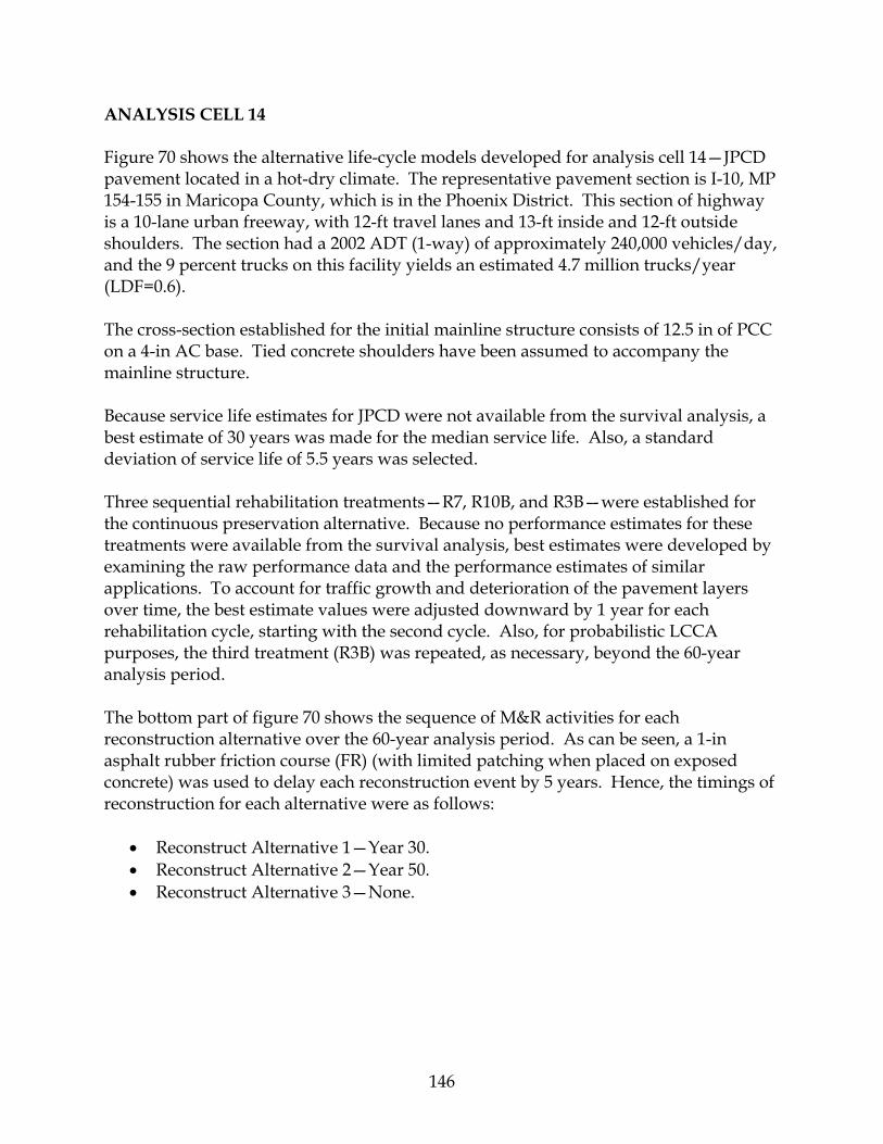
146
ANALYSIS CELL 14 Figure 70 shows the alternative life-cycle models developed for analysis cell 14—JPCD pavement located in a hot-dry climate. The representative pavement section is I-10, MP 154-155 in Maricopa County, which is in the Phoenix District. This section of highway is a 10-lane urban freeway, with 12-ft travel lanes and 13-ft inside and 12-ft outside shoulders. The section had a 2002 ADT (1-way) of approximately 240,000 vehicles/day, and the 9 percent trucks on this facility yields an estimated 4.7 million trucks/year (LDF=0.6). The cross-section established for the initial mainline structure consists of 12.5 in of PCC on a 4-in AC base. Tied concrete shoulders have been assumed to accompany the mainline structure. Because service life estimates for JPCD were not available from the survival analysis, a best estimate of 30 years was made for the median service life. Also, a standard deviation of service life of 5.5 years was selected. Three sequential rehabilitation treatments—R7, R10B, and R3B—were established for the continuous preservation alternative. Because no performance estimates for these treatments were available from the survival analysis, best estimates were developed by examining the raw performance data and the performance estimates of similar applications. To account for traffic growth and deterioration of the pavement layers over time, the best estimate values were adjusted downward by 1 year for each rehabilitation cycle, starting with the second cycle. Also, for probabilistic LCCA purposes, the third treatment (R3B) was repeated, as necessary, beyond the 60-year analysis period. The bottom part of figure 70 shows the sequence of M&R activities for each reconstruction alternative over the 60-year analysis period. As can be seen, a 1-in asphalt rubber friction course (FR) (with limited patching when placed on exposed concrete) was used to delay each reconstruction event by 5 years. Hence, the timings of reconstruction for each alternative were as follows:
• Reconstruct Alternative 1—Year 30. • Reconstruct Alternative 2—Year 50. • Reconstruct Alternative 3—None.

147
Activity Sequence for Reconstruction Alternatives Year Reconstruct Alt. #1 Reconstruct Alt. #2 Reconstruct Alt. #3
30 M2B (FR) (5.0 ± 0.0 yrs) 1” FR (1” AC) 1% PDR (AC) (0.2% PDR (AC)) 1% FDR (0.2% FDR)
R7 (GR) (15.0 ± 3.5 yrs) 0.5% PDR (0.1% PDR) 5% FDR (1% FDR) 100% GR T/L Jt Seal (T/L Jt Seal)
R7 (GR) (15.0 ± 3.5 yrs) 0.5% PDR (0.1% PDR) 5% FDR (1% FDR) 100% GR T/L Jt Seal (T/L Jt Seal)
30 JPCD (Reconstruct) (30.0 ± 5.5 yrs) 13” PC (13” PC) 4” AC (4” AC) 17.5” RE (17.5” RE)
45 M2B (FR) (5.0 ± 0.0 yrs) 1” FR (1” AC) 1% PDR (AC) (0.2% PDR (AC)) 1% FDR (0.2% FDR)
R1B (AR+FR) (13.0 ± 2.75 yrs) 1” FR (3” AC) 2” AR 2% PDR (AC) (1% PDR (AC)) 5% FDR (1% FDR)
50 JPCD (Reconstruct) (30.0 ± 5.5 yrs) 13.5” PC (13.5” PC) 4” AC (4” AC) 17.5” RE (17.5” RE)
58 M2B (RE+FR) (5.0 ± 0.0 yrs) 1” FR 1” RE
60 M2B (FR) (5.0 ± 0.0 yrs) 1” FR (1” AC) 1% PDR (AC) (0.2% PDR (AC)) 1% FDR (0.2% FDR)
Figure 70. Life-cycle models for analysis cell 14—JPCD pavement, hot-dry climate.
JPCD (new) 12.5” PC (12.5” PC) 4” AC (4” AC)
Maint 0.5% FDR T/L Jt Seal (T/L Jt Seal)
R7 (GR) 0.5% PDR (0.1% PDR) 5% FDR (1% FDR) 100% GR T/L Jt Seal (T/L Jt Seal)
R1B (AR+FR) 1” FR (3” AC) 2” AR 2% PDR (AC) (1% PDR (AC)) 5% FDR (1% FDR) 30.0 + 5.5 yrs
15.0 + 3.5 yrs 13.0 + 2.75 yrs
Every 15 yrs
0 10 20 30 40 50 60
Continuous Preservation Alternative
Every 7 yrs
Maint 0” FL
R3B (RE+AC+FR) 0.5” FR (1.5” AC) 2” AC 1” RE
10.0 + 2.5 yrs
Maint 0” FL
Every 7 yrs
Maint 0.5% FDR
Every 10 yrs

148
ANALYSIS CELL 15 Figure 71 shows the alternative life-cycle models developed for analysis cell 15—CRC pavement located in a hot-dry climate. The representative pavement section is SR 101L, MP 11-12 in Maricopa County, which is in the Phoenix District. This section of highway is a 6-lane urban freeway, with 12-ft travel lanes and 8-ft inside and 10-ft outside shoulders. The section had a 2002 ADT (1-way) of approximately 75,000 vehicles/day, and the 4 percent trucks on this facility yields an estimated 0.9 million trucks/year (LDF=0.8). The cross-section established for the initial mainline structure consists of 10 in of PCC on a 6-in aggregate base. Tied concrete shoulders have been assumed to accompany the mainline structure. Because service life estimates for CRC were not available from the survival analysis, a best estimate of 34 years was made for the median service life. Also, a standard deviation of service life of 6.5 years was selected. Two sequential rehabilitation treatments—R1B and R3B—were established for the continuous preservation alternative. Because no performance estimates for these treatments were available from the survival analysis, best estimates were developed by examining the raw performance data and the performance estimates of similar applications. To account for traffic growth and deterioration of the pavement layers over time, the best estimate values were adjusted downward by 1 year for each rehabilitation cycle, starting with the second cycle. Also, for probabilistic LCCA purposes, the third treatment (R3B) was repeated, as necessary, beyond the 60-year analysis period. The bottom part of figure 71 shows the sequence of M&R activities for each reconstruction alternative over the 60-year analysis period. As can be seen, a 1-in asphalt rubber friction course (FR) (with limited patching when placed on exposed concrete) was used to delay each reconstruction event by 5 years. Hence, the timings of reconstruction for each alternative were as follows:
• Reconstruct Alternative 1—Year 39. • Reconstruct Alternative 2—Year 54. • Reconstruct Alternative 3—None.

149
Activity Sequence for Reconstruction Alternatives Year Reconstruct Alt. #1 Reconstruct Alt. #2 Reconstruct Alt. #3
34 M2B (FR) (5.0 ± 0.0 yrs) 1” FR (1” AC) 1% PDR (AC) (0.2% PDR (AC)) 1% FDR (0.2% FDR)
R1B (AR+FR) (15.0 ± 3.0 yrs) 0.5% FR (2” AC) 1.5” AR 0.5% PDR (AC) (0.1% PDR (AC)) 5% FDR (1% FDR)
R1B (AR+FR) (15.0 ± 3.0 yrs) 0.5% FR (2” AC) 1.5” AR 0.5% PDR (AC) (0.1% PDR (AC)) 5% FDR (1% FDR)
39 CRC (Reconstruct) (34.0 ± 5.5 yrs) 10.5” PC (10.5” PC) 6” AB (6” AB) 17” RE (17” RE)
49 M2B (FR) (5.0 ± 0.0 yrs) 1” FR (1” AC) 1% PDR (AC) (0.2% PDR (AC)) 1% FDR (0.2% FDR)
R3B (RE+AR=FR) (13.0 ± 2.5 yrs) 0.75” FR (0.25” SC) 2” AR 2” RE 1% PDR (AC) 5% FDR
54 CRC (Reconstruct) (34.0 ± 6.5 yrs) 11” PC (11” PC) 6” AB (6” AB) 19” RE (19” RE)
Figure 71. Life-cycle models for analysis cell 15—CRC pavement, hot-dry climate.
CRC (new) 10” PC (10” PC) 6” AB (6” AB)
Maint 0.5% FDR L Jt Seal (L Jt Seal)
R1B (AR+FR) 0.5” FR (2” AC) 1.5” AR 0.5% PDR (AC) (0.1% PDR (AC)) 5% FDR (1% FDR)
R3B (RE+AR+FR) 0.75” FR (0.25” SC) 2” AR 2” RE 1% PDR (AC) 5% FDR 34.0 + 6.5 yrs
15.0 + 3.0 yrs 13.0 + 2.5 yrs
Every 15 yrs
0 10 20 30 40 50 60
Continuous Preservation Alternative
Every 7 yrs
Maint 0” FL
Every 7 yrs
Maint 0” FL

150

151
CHAPTER 7. LIFE-CYCLE COST ANALYSIS INTRODUCTION This chapter provides a discussion of the life-cycle cost analyses (LCCAs) performed to determine the cost-effectiveness of continuous pavement preservation and the break-even point between the continuous preservation and reconstruction strategies. The discussion covers the LCCA approach and software used to compute life-cycle costs for the alternative strategies, the various LCCA inputs (e.g., project details, analysis options, traffic data, value of user time) utilized in the analyses, and the subsequent results. LCCA APPROACH AND SOFTWARE For the economic analyses required by this study, a probabilistic approach was taken using the FHWA’s LCCA spreadsheet program, RealCost Version 2.1 (FHWA, 2004). Probabilistic LCCA is a simulation technique that accounts for the real-world variability and/or uncertainty associated with the various input parameters (e.g., costs, performance) that are used to compute life-cycle costs. The process entails defining individual input parameters by a frequency (or probability) distribution (rather than by discrete values, as is done in deterministic LCCA) and computing an array of life-cycle costs through iterative sampling of the pre-defined frequency distributions of each input variable. The resulting array of life-cycle costs form a unique probability distribution, which can then be examined and compared with the cost distribution of a competing design alternative. RealCost was developed by the FHWA in 2002/2003 to support the application of LCCA in the pavement project-level decision-making process. This Microsoft® Excel-based program is built on the principles and best practices outlined in the FHWA’s Interim Technical Bulletin on LCCA (Walls and Smith, 1998) and it utilizes the Visual Basic programming functions available within Excel. The program can perform both deterministic and probabilistic modeling and can compute both agency and user (work zone-related) life-cycle costs. The life-cycle costs are in the form of net present value (NPV), which is computed as follows: Eq. 9 where: NPV = Net present value, $. i = Discount rate, percent. n = Time of future cost, years.
( )∑ ⎥⎦
⎤⎢⎣
⎡
++= ni
CostFutureCostInitialNPV1
1*

152
The simulation technique utilized by RealCost for probability simulation is the Monte Carlo simulation. As illustrated in figure 72, the Monte Carlo simulation draws values from the probability distributions for each uncertain input variable, and uses these values to compute a single NPV output value. Note that a single iteration of the simulation process represents one possible scenario or outcome. The process of sampling from a probability distribution is repeated until the specified number of iterations is completed or until the simulation process converges. The simulation converges at the point where additional iterations do not significantly change the output distribution (Walls and Smith, 1998).
Figure 72. NPV distribution generation (Walls and Smith, 1998). LCCA INPUTS Well-developed inputs for the RealCost LCCA spreadsheet program are necessary to predict accurate life-cycle costs for pavement alternatives (pavement preservation design or reconstruction approach strategies as discussed in chapter 6) using a probabilistic-based analysis. Provided in the sections below are presentations of the input values used in performing the LCCAs and discussions of how they were derived. For this study, a normal probability distribution was used for all probabilistic inputs. Moreover, a total of 1,000 simulations were performed for each LCCA. Only two alternatives per LCCA could be considered due to the makeup and structure of the RealCost program. For each LCCA, the resulting life-cycle cost distributions for each alternative were compared to determine the more economical alternative.
153
Project Details The following inputs were entered into the Project Detail module of RealCost to accurately define the projects and design alternatives presented in chapter 6:
• State Route. • Project Name. • Region (ADOT District). • County. • Analyzed By. • Begin Milepost. • End Milepost. • Lane Width. • Shoulder Width.
Analysis Options The following inputs and selections were made as part of the Analysis Options module of RealCost:
• Analysis Period—The analysis period is defined as the time period over which the initial and future costs are evaluated for different design alternatives. For the primary assessment of life-cycle costs, a uniform analysis period of 60 years was used, since examinations of up to three reconstruction events were considered. Shorter analysis periods of 40 and 50 years were used for a couple scenarios to examine the impact of analysis period on the life-cycle costs of continuous preservation and reconstruction.
• Discount Rate—The discount rate is very important because it can significantly influence the results of the analysis. The discount rate is a function of both the interest rate and inflation rate. For the primary assessment of life-cycle costs, a discount rate of 4 percent with a standard deviation of 0.4 percent was used to best represent the time value of money. For sensitivity analysis purposes, discount rates of 0, 4, and 8 were used in a couple scenarios.
• Beginning of Analysis Period—The current year (2004) was defined as the beginning of the analysis period.
• Include Agency Cost Residual Value—This option was selected to include salvage value representing the remaining serviceable life of an alternative at the end of the analysis period. The salvage value is calculated as the percentage of the design life remaining at the end of the analysis period multiplied by the cost of the last rehabilitation of the alternative.
• Include User Costs in Analysis—This option was selected to include work zone-related user costs in the analysis.

154
• User Cost Computation Method—“Calculated” was selected to allow the work zone related user cost to be computed by the LCCA2002 program. “Specified” can be selected so that manually computed user costs can be entered in Alternative 1 and/or Alternative 2 modules.
• Traffic Direction—“Both” was selected to include analysis of rehabilitation of both directions of the project section. “Inbound” can be selected to analyze the inbound direction or “Outbound” can be selected to analyze the outbound direction of the project section.
• Include User Costs Residual Value—This option, which is a new concept, allows the user to indicate whether the residual value of the user cost associated with the last rehabilitation of an alternative should be accounted for when the last rehabilitation is expected to last beyond the analysis period. User cost residual value is calculated as the total user cost during the last rehabilitation multiplied by the percentage of the remaining life of the last rehabilitation. This option was not selected due to unfamiliarity with its consequences on life-cycle costs.
Table 47 summarizes the selections made in the Analysis Options module.
Table 47. Summary of the selections made for the Analysis Options module.
Input Variable Value
Analysis period, yrs 60 (40 and 50 also examined)
Include User Costs in Analysis Yes Include User Cost Remaining Service Life Value No Use Differential User Costs Yes User Cost Computation Method Calculated Include Agency Cost Remaining Service Life Value Yes Traffic Direction Both Beginning of Analysis Period 2004
Discount Rate, percent 4 (0 and 8 also examined)
Traffic Data The following inputs define the traffic data for both the continuous preservation and reconstruction pavement strategies.
• AADT (Both Directions) Construction Year—Annual average daily traffic for both directions of roadway corresponding to the initial construction year. Each AADT value entered was for the specific roadway section selected for the analysis cell.
155
• Single Trucks as Percentage of AADT Year—Number of single-unit trucks as a percentage of AADT for both directions of the roadway. Each percentage of single trucks entered was for the specific roadway section selected for the analysis cell.
• Combo Unit Trucks as Percentage of AADT Year—Number of combination-unit trucks as a percentage of AADT for both directions of the roadway. Each percentage of combination unit trucks entered was for the specific roadway section selected for the analysis cell.
• Annual Growth of Traffic—Annual growth rate of traffic in percent. A 2.5 percent average growth rate with a standard deviation 0.4 percent was entered for each analysis cell.
• Speed Limit Under Normal Conditions—Speed limit (in miles per hour [mi/hr]) under normal conditions or when a work zone is not in place. The current Arizona State maximum speed limit of 75 mi/hr for rural freeways and 55 mi/hr for divided highway, undivided highway, and urban freeway was entered for the normal condition speed limit.
• Lanes Open in Each Direction Under Normal Operation Year—Number of lanes open during normal operations. The maximum number of lanes was entered for the specific roadway section selected for the analysis cell.
• Free Flow Capacity—Free flow capacity is the maximum capacity, in vehicles per hour per lane (vphpl) a facility can handle under free flow conditions. Free flow capacity was used in calculating user costs when there was no work zone in place or queue. Free flow capacity is a function of number of factors, including number and width of lanes, shoulder widths, terrain of the roadway and traffic composition.
• Queue Dissipation Capacity—Queue dissipation capacity is the capacity of the roadway, in vehicles per hour per lane (vphpl), when a queue has been formed and is dissipating. Queue dissipation capacity was less than the free flow capacity, even though all lanes were available for traffic. Queue dissipation capacity is used in calculating user costs whenever a queue has been formed and is dissipating.
• Maximum AADT (Both Directions)—When existing traffic and expected growth rate are high, calculated future traffic that is determined from existing AADT compounded by AADT growth rate, could exceed the capacity of the roadway over a 24-hour period. This is not practically possible and is a limitation of the assumptions made regarding the growth rate, future traffic behavior or capacity improvements. The maximum AADT can be used to cap the future AADT at some reasonable levels. It should be less than the 24-hour capacity of the roadway. If this is higher than the 24-hour capacity, future AADT will be capped using an estimated 24-hour capacity in the analysis.
• Maximum Queue Length—Practical maximum length of queue in miles (mi). User costs are calculated on an hourly basis and when the demand (traffic volume) exceeds capacity, queue begins to form. As long as this condition prevails, the queue will continue to grow and may results in calculated or

156
theoretical queue lengths that are quite large and not practical. When queue length becomes significantly long, what is a long queue varies based on network level traffic condition and other factors, some redistribution of traffic will occur. In these cases, the maximum queue length is intended to account for this in an approximate manner. The maximum queue length could be one or two exits prior to the work zone or an exit that leads to a reasonable alternate route. Calculated queue length is capped at the maximum queue length.
• Rural/Urban Year—Specifies whether the project section is located in a rural or urban area. The entry for this field was specific to the roadway section selected for the analysis cell.
The traffic information used in the analyses was specific to the project being evaluated. A summary of the selected inputs is presented in table 48. Value of User Time The following inputs define the value of user time for both the continuous preservation and reconstruction pavement strategies:
• Value of Time for Passenger Cars—Economic value of time for passenger cars, expressed in $/hour, reflects the added cost to passenger cars due to time lost in traveling through work zone. Recommended range for value of time for passenger cars is $10 to $13/hour (Walls and Smith, 1998).
• Value of Time for Single-Unit Trucks—Economic value of time for single-unit trucks, expressed in $/hour, reflects the added cost to single unit trucks due to time lost in traveling through work zone. Recommended range for value of time for single unit trucks is $17 to $20/hour (Walls and Smith, 1998).
• Value of Time for Combination Unit Trucks—Economic value of time for combination trucks, expressed in $/hour, reflects the added cost to combination trucks due to time lost in traveling through work zone. Recommended range for value of time for combination trucks is $21 to $24/hour (Walls and Smith, 1998).
Traffic Hourly Distribution Since directional hourly traffic distribution data were not available for each of the projects analyzed, the default hourly distributions for various roadway types in urban and rural settings from MicroBenCost was used in this module (NCHRP 1995). The default hourly distribution used is shown in figure 73 for rural and urban project site locations.
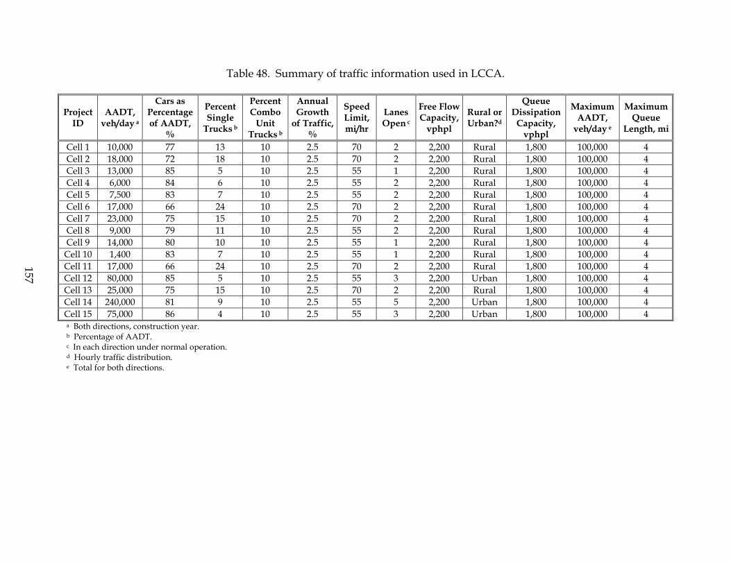
Table 48. Summary of traffic information used in LCCA.
Project ID
AADT, veh/day a
Cars as Percentage of AADT,
%
Percent Single
Trucks b
Percent Combo
Unit Trucks b
Annual Growth
of Traffic, %
Speed Limit, mi/hr
Lanes Open c
Free Flow Capacity,
vphpl
Rural or Urban?d
Queue Dissipation
Capacity, vphpl
Maximum AADT,
veh/day e
Maximum Queue
Length, mi
Cell 1 10,000 77 13 10 2.5 70 2 2,200 Rural 1,800 100,000 4 Cell 2 18,000 72 18 10 2.5 70 2 2,200 Rural 1,800 100,000 4 Cell 3 13,000 85 5 10 2.5 55 1 2,200 Rural 1,800 100,000 4 Cell 4 6,000 84 6 10 2.5 55 2 2,200 Rural 1,800 100,000 4 Cell 5 7,500 83 7 10 2.5 55 2 2,200 Rural 1,800 100,000 4 Cell 6 17,000 66 24 10 2.5 70 2 2,200 Rural 1,800 100,000 4 Cell 7 23,000 75 15 10 2.5 70 2 2,200 Rural 1,800 100,000 4 Cell 8 9,000 79 11 10 2.5 55 2 2,200 Rural 1,800 100,000 4 Cell 9 14,000 80 10 10 2.5 55 1 2,200 Rural 1,800 100,000 4
Cell 10 1,400 83 7 10 2.5 55 1 2,200 Rural 1,800 100,000 4 Cell 11 17,000 66 24 10 2.5 70 2 2,200 Rural 1,800 100,000 4 Cell 12 80,000 85 5 10 2.5 55 3 2,200 Urban 1,800 100,000 4 Cell 13 25,000 75 15 10 2.5 70 2 2,200 Rural 1,800 100,000 4 Cell 14 240,000 81 9 10 2.5 55 5 2,200 Urban 1,800 100,000 4 Cell 15 75,000 86 4 10 2.5 55 3 2,200 Urban 1,800 100,000 4 a Both directions, construction year. b Percentage of AADT. c In each direction under normal operation. d Hourly traffic distribution. e Total for both directions.
157

158
Figure 73. Default hourly distribution used in analysis (for rural and urban project site locations).
Added Vehicle Time and Cost The default added time and vehicle running cost per 1000 stops and idling costs were used for this module. The costs were escalated to the year 2003 using the built-in function. Alternative-Level Inputs The following inputs describe each of the pavement alternatives compared in the LCCAs. Each alternative included an initial construction and six rehabilitation/ reconstruction events/activities. Alternative Description The alternative description identifies the pavement alternative (continuous preservation, reconstruction with no prior rehabilitations, reconstruction with 1 prior rehabilitation, reconstruction with 2 prior rehabilitations), pavement type (CAC, DSAC/FDAC, JPC, JPCD, and CRC), county in which the project is located, route name, begin and end milepost, and climate type (hot-dry, moderate, and cool-wet).
0
1
2
3
4
5
6
7
8
9
10
12:3
0:00
AM
2:30
:00
AM
4:30
:00
AM
6:30
:00
AM
8:30
:00
AM
10:3
0:00
AM
12:3
0:00
PM
2:30
:00
PM
4:30
:00
PM
6:30
:00
PM
8:30
:00
PM
10:3
0:00
PM
Hou
rly tr
affic
dis
tribu
tion,
per
cent
AA
DT Rural
Urban
159
Activity Description
The activity description identifies the construction or rehabilitation activity. The activity description defines whether the activity is new construction or a preservation activity. The activity description also includes the cross-section of the pavement. Agency Construction Costs The agency construction costs are the individual costs (in $1,000) of the initial pavement structure and each of the subsequent rehabilitation/reconstruction events/activities. These costs were computed using the estimated pay item unit costs listed in table 49 (derived from the analyses of unit costs discussed in chapter 4) and the pay item quantities projected for each event/activity. For the probabilistic LCCA, a standard deviation of 12 percent was applied to each event/activity cost. Additional cost items used in the LCCAs were as follows:
• Traffic control costs—Average daily cost of traffic control, including Traffic Control Labor (4 people, 10 hr days), Sequential Arrow Sign, and Traffic Control Supervisor. A daily cost of $1,080 was used.
• Mobilization—An average mobilization cost of 5 percent of the project total cost was used.
• Sales Tax—An average sales tax of 7.6 percent of the project total cost was used. • Engineering and Contingencies—An average engineering and contingency cost
of 15 percent of the project total cost was used. • Preliminary engineering costs—An average preliminary engineering cost of 10
percent of the total construction cost was used. Activity Service Life The activity service life represents the expected life of the initial pavement structure or the rehabilitated/reconstructed pavement. For this investigation, the service life values used were those defined in the life-cycle models developed and presented in chapter 6. The values were derived from the results of the comprehensive pavement performance analyses described in chapter 3. User Work Zone Costs The user work zone costs is the total user cost (in $1,000) of the initial or rehabilitation activities, when "Specified" option is selected for User Cost Computation in the Analysis Options module. This input is disabled when "Calculated" option is selected for User Cost Computation. The User Cost Computation was specified as “Calculated” for all analysis in this study. Table 50 presents a summary of the user work zone unit costs used in the LCCAs.

160
Table 49. Summary of pay item unit costs used to estimate event/activity costs.
Bid Item Unit Description Bid Item Components Unit Price Quantity Per Day
ton Asphalt Concrete Friction Course $28.13
ton Asphalt Cement for ACFC $154.03 Asphalt Concrete Friction Course (FC)
ton Mineral Admixture for ACFC $97.42
2,000
ton Asphalt Rubber AC Friction Course $29.44
ton Asphalt Cement for AR-ACFC $274.99 Asphalt Rubber AC Friction Course (FR)
ton Mineral Admixture for AR-ACFC $97.42
2,000
ton Asphalt Concrete (3/4" Mix) $22.09
ton Asphalt Cement for AC (3/4" Mix) $154.03 Asphalt Concrete (AC)
ton Mineral Admixture for AC (3/4" Mix) $97.42
2,000
ton Asphalt Rubber AC $25.65
ton Asphalt Cement for AR-AC $260.48 Asphalt Rubber AC (AR)
ton Mineral Admixture for AR-AC $97.42
2,000
ton Asphalt Concrete (Base Mix) $19.66
ton Asphalt Cement for AC (Base Mix) $154.03 Asphalt Concrete (Base Mix)
ton Mineral Admixture for AC (Base Mix) $97.42
2,000
ton Recycled AC $18.00
ton Asphalt Cement for Recycled AC $158.17 Recycled AC (RO)
ton Mineral Admixture for Recycled AC $97.42
2,000
ton Emulsified Asphalt (CRS-2) $180.37 40 Seal Coat (SC)
yd3 Cover Material $40.68 800
ton Asphalt for Tack Coat $163.44 Tack Coat
hr Apply Tack Coat $114.25 —
Prime Coat ton Asphalt for Prime Coat $222.79 —
ft2 Partially Depth Repairs $15.51 —
yd2 Full Depth Repairs $207.83 —
yd2 Grind Existing PCC Pavement $10.25 —
ft Longitudinal Joint Seal $0.95 —
Concrete pavement repair (CPR)
ft Transverse Joint Seal $2.43 — Aggregate Base (AB), Class 2 yd3 Aggregate Base, Class 2 $23.70 2,500
Aggregate Subbase (SM, SB), Class 6 yd3 Aggregate Subbase, Class 6 $17.32 2,500
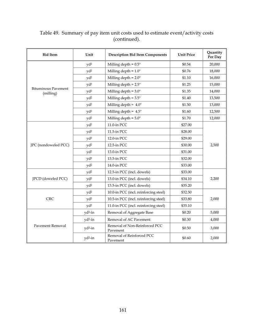
161
Table 49. Summary of pay item unit costs used to estimate event/activity costs (continued).
Bid Item Unit Description Bid Item Components Unit Price Quantity Per Day
yd2 Milling depth = 0.5" $0.54 20,000
yd2 Milling depth = 1.0" $0.76 18,000
yd2 Milling depth = 2.0" $1.10 16,000
yd2 Milling depth = 2.5" $1.25 15,000
yd2 Milling depth = 3.0" $1.35 14,000
yd2 Milling depth = 3.5" $1.40 13,500
yd2 Milling depth = 4.0" $1.50 13,000
yd2 Milling depth = 4.5" $1.60 12,500
Bituminous Pavement (milling)
yd2 Milling depth = 5.0" $1.70 12,000
yd2 11.0-in PCC $27.00
yd2 11.5-in PCC $28.00
yd2 12.0-in PCC $29.00
yd2 12.5-in PCC $30.00
yd2 13.0-in PCC $31.00
yd2 13.5-in PCC $32.00
JPC (nondoweled PCC)
yd2 14.0-in PCC $33.00
2,500
yd2 12.5-in PCC (incl. dowels) $33.00
yd2 13.0-in PCC (incl. dowels) $34.10 JPCD (doweled PCC)
yd2 13.5-in PCC (incl. dowels) $35.20
2,200
yd2 10.0-in PCC (incl. reinforcing steel) $32.50
yd2 10.5-in PCC (incl. reinforcing steel) $33.80 CRC
yd2 11.0-in PCC (incl. reinforcing steel) $35.10
2,000
yd2-in Removal of Aggregate Base $0.20 5,000
yd2-in Removal of AC Pavement $0.30 4,000
yd2-in Removal of Non-Reinforced PCC Pavement $0.50 3,000 Pavement Removal
yd2-in Removal of Reinforced PCC Pavement $0.60 2,000

162
Table 50. Summary of user work zone unit costs.
Parameter Cost Value of Time for Passenger Cars ($/hour) $3.08 Value of Time for Single Unit Trucks ($/hour) $20.95 Value of Time for Combination Trucks ($/hour) $25.21
Maintenance Frequency The maintenance frequency is the interval (in years) between routine maintenance activities. A zero is entered when no routine maintenance is included with an initial construction or rehabilitation. The maintenance frequency entered for all analysis cells’ alternatives was specific for each initial construction or rehabilitation. Agency Maintenance Costs Agency maintenance costs are the routine maintenance costs (in $1,000) for the initial or rehabilitation activities. The agency maintenance costs are applied at the interval specified in the maintenance frequency for the duration of particular activity's life. The agency maintenance costs were calculated in Microsoft® Excel spreadsheets outside of the RealCost program using bid items, unit costs, and mainline and shoulder widths for the specific design section selected for each analysis cell. An example maintenance calculation for a JPCD design section with 1% full-depth repairs (FDR), 100% diamond grinding (GR), and longitudinal joint sealing is shown table 51.
Table 51. Example calculation of agency maintenance costs.
Length (ft) Width (ft) Area (yd2) Percent Unit Cost ($/yd2) Average Cost ($) Std. Dev. Cost ($)5,280 72 42,240 1 207.83 $87,7875,280 72 42,240 1 --- ---
Length (ft) Width (ft) Area (yd2) Percent Unit Cost ($/yd2) Average Cost ($) Std. Dev. Cost ($)5,280 72 42,240 100 2.62 $110,6695,280 72 42,240 100 --- ---
Length (ft) Width (ft) Length (LF) Percent Unit Cost ($/ft) Average Cost ($) Std. Dev. Cost ($)5,280 72 42,240 100 0.95 $40,1285,280 72 42,240 100 0.09 $3,802
$238,584Total Maintenance Cost
Mainline Maintenance Activity - 1% Full Depth Repair
Mainline Maintenance Activity - 100% Groove Existing JPCD Pavement
Mainline Maintenance Activity - Longitudinal Joint Seal

163
Work Zone Length The work zone is the length of section (in miles [mi]) where the work zone is in place. When large sections of roadway are rehabilitated, construction proceeds in sequence and the work zone is in place only for only a portion of the project. For all analyses, a work zone length of 1 mi was used. Work Zone Duration The work zone duration is the total number of days the work zone will be in place to complete the initial or rehabilitation activity for the entire project length. The work zone duration includes all days that the work zone will be in place (restricted travel conditions) and is not limited to the days of construction activity. The work zone duration is the summation of the estimated individual duration of each pay item for the project. The work zone duration was calculated for both alternatives for each analysis cell in an Alternative Agency Cost worksheet. Work Zone Speed Limit The work zone speed limit is the speed limit (in miles per hour [mi/hr]) during work zone. The work zone speed limit must be less than the speed limit under normal operating conditions. A work zone speed limit of 45 mi/hr was used for all analysis cells. Number of Lanes Open in Each Direction During Work Zone The number of lanes open in each direction during work zone is used to calculate the capacity of the roadway when a work zone is in place and cannot be higher than the number of lanes in each direction of the roadway. The number of lanes open in each direction is 1 less than the total number of lanes in each direction for all analysis cells. Period of Lane Closure Three different periods of work zone hours can be specified for each inbound and outbound direction of the roadway. If only one direction of the roadway is being analyzed, then only the number of hours related to that direction needs to be provided. The number of hours needs to be entered using a 24-hour clock. For example, if a work zone is put in place from 10 PM to 5 AM the next day, then this should be entered using two periods as follow: Period 1: 0 hours to 5 hours and Period 2: 22 hours to 24 hours. For all the cells analyzed, the period of lane closure was 9 AM to 5 PM.

164
SUMMARY OF LCCA RESULTS A detailed summary of the results of the LCCA is presented for all 15 cells in table 52. This table shows the NPV for each alternative (see chapter 6) at both the mean (50 percent) and 90 percent probability. Figures 74 through 88 provide plots of agency and user costs for each iteration within a given analysis cell. Sensitivity Analysis A sensitivity analysis was done by varying the value of critical parameters to determine their impact on cost. This was done at two levels: (1) the impact of critical parameters on estimated cost (NPV) and (2) the impact of critical parameters on optimal timing of reconstruction. At the first level, the critical parameters evaluated included:
• Initial construction cost. • Initial construction life. • Initial construction work zone duration. • Queue dissipation capacity. • Rehabilitation construction cost. • Rehabilitation construction life. • Rehabilitation construction work zone duration.
A summary of the four most significant parameters for analysis cell 3 (2-lane, CAC) and analysis cell 12 (6-lane, JPC) were (1) initial construction cost, (2) initial construction life, (3) discount rate, and (4) value of time for passenger cars. For the second level of sensitivity analysis the effect of two critical parameters, namely discount rate and analysis period, on costs and, hence the optimal timing of reconstruction, was evaluated. The ranges of the critical parameters evaluated are as follows:
• Discount rate—0, 4, and 8 percent. • Analysis period—40-, 50-, and 60-years.
The results of the evaluation are presented in figures 89 and 90.

Table 52. Summary of NPV at mean (50 percent) and 90 percent probability.
Estimated Cost @ 50 percent Probability, $1,000 Std. Dev., $1,000 Estimated Cost @ 90 percent
Probability, $1,000 Project ID
Analysis Type Alt.
Total Agency User Agency User Total Agency User
Mean Cost, $1,000
Difference in Cont. Pres. and Reconst.
Alt. Cost, %1 1 1,815.87 1,768.56 47.31 216.59 18.44 2,203.67 2,125.93 77.74 2 1,833.14 1,783.21 49.93 215.29 19.39 2,220.36 2,138.44 81.92
Cont. Pres.
3 1,769.01 1,720.69 48.32 219.4 18.5 2,161.55 2,082.70 78.85 2,195.19 —
1 2,294.65 2,231.20 63.45 284.59 29.33 2,812.62 2,700.77 111.84 2,812.62 +28.13 2 1,970.10 1,925.41 44.69 234.54 10.62 2,374.61 2,312.40 62.21 2,374.61 +8.17
Cell 1 (CAC)
Reconst. 3 1,815.01 1,762.14 52.87 220.95 24.43 2,219.89 2,126.71 93.18 2,219.89 +1.13 1 2,332.58 2,068.78 263.80 217.96 85.18 2,832.76 2,428.41 404.35 2 2,336.04 2,079.38 256.66 205.81 82.29 2,811.41 2,418.97 392.44 Cont.
Pres. 3 2,344.62 2,078.63 265.99 215.35 79.68 2,831.42 2,433.96 397.46
2,825.20 —
1 3,563.12 3,016.95 546.17 359.74 223.68 4,525.76 3,610.52 915.24 4,525.76 +60.19 2 2,721.32 2,422.70 298.62 257.22 143.24 3,382.08 2,847.11 534.97 3,382.08 +19.71
Cell 2 (CAC)
Reconst. 3 2,847.53 2,295.65 551.88 261.04 184.04 3,581.91 2,726.37 855.55 3,581.91 +26.78 1 1,457.49 1,188.50 268.99 139.81 60.08 1,787.31 1,419.19 368.12 2 1,469.81 1,197.35 272.46 136.03 63.70 1,799.36 1,421.80 377.57 Cont.
Pres. 3 1,465.77 1,195.18 270.59 140.49 60.41 1,797.26 1,426.99 370.27
1,794.64 —
1 2,027.30 1,527.84 499.46 221.81 136.86 2,619.11 1,893.83 725.28 2,619.11 +45.94 2 1,728.11 1,331.65 396.46 192.44 90.95 2,195.70 1,649.18 546.53 2,195.70 +22.34
Cell 3 (CAC)
Reconst. 3 1,508.28 1,204.61 303.67 156.53 115.41 1,956.98 1,462.88 494.10 1,956.98 +9.05 1 1,021.50 1,017.44 4.06 115.60 0.42 1,212.93 1,208.18 4.75 2 1,024.53 1,020.46 4.07 107.64 0.44 1,202.86 1,198.07 4.80 Cont.
Pres. 3 1,028.70 1,024.62 4.08 116.28 0.43 1,221.27 1,216.48 4.79
1,212.36 —
1 1,281.70 1,275.72 5.98 182.88 1.19 1,585.42 1,577.47 7.94 1,585.42 +30.77 2 1,073.38 1,068.45 4.93 151.81 1.22 1,325.88 1,318.94 6.94 1,325.88 +9.36
Cell 4 (CAC)
Reconst. 3 1,019.72 1,015.65 4.07 115.18 0.51 1,210.61 1,205.70 4.91 1,210.61 -0.14
1 Positive value means continuous preservation is less expensive alternative. Negative value means reconstruction is less expensive alternative.
165

Table 52. Summary of NPV at mean (50 percent) and 90 percent probability (continued).
Estimated Cost @ 50 percent Probability, $1,000 Std. Dev., $1,000 Estimated Cost @ 90 percent
Probability, $1,000 Project ID
Analysis Type Alt.
Total Agency User Agency User Total Agency User
Mean Cost, $1,000
Difference in Cont. Pres. and Reconst.
Alt. Cost, %1 1 1,551.11 1,544.46 6.65 172.97 0.96 1,838.09 1,829.86 8.23 2 1,553.48 1,546.89 6.59 159.69 0.83 1,818.34 1,810.38 7.96
Cont. Pres.
3 1,559.91 1,553.28 6.63 172.02 0.82 1,845.10 1,837.11 7.98 1,833.84
—
1 2,274.14 2,260.99 13.15 329.44 3.55 2,823.57 2,804.57 19.01 2,823.57 +53.97 2 1,794.58 1,785.12 9.46 253.37 2.02 2,215.97 2,203.18 12.79 2,215.97 +20.84
Cell 5 (CAC)
Reconst.
3 1,569.90 1,562.57 7.33 189.25 2.72 1,886.65 1,874.83 11.82 1,886.65 +2.88 1 3,001.77 2,409.70 592.07 266.00 176.65 3,732.14 2,848.60 883.54 2 3,001.77 2,409.70 592.07 266.00 176.65 3,732.14 2,848.60 883.54
Cont. Pres.
3 3,024.55 2,423.54 601.01 262.55 179.35 3,753.69 2,856.75 896.94 3,739.32
—
1 4,003.26 3,172.20 831.06 340.19 220.44 4,928.30 3,733.51 1,194.79 4,928.30 +31.79 2 3,651.11 2,734.17 916.94 313.35 323.78 4,702.37 3,251.20 1,451.18 4,702.37 +25.75
Cell 6 (DSAC)
Reconst.
3 3,341.92 2,514.24 827.68 286.92 201.55 4,147.90 2,987.66 1,160.24 4,147.90 +10.92 1 2,592.61 2,318.62 273.99 257.13 105.07 3,190.24 2,742.88 447.36 2 2,613.58 2,334.88 278.70 250.09 102.79 3,195.83 2,747.53 448.30
Cont. Pres.
3 2,612.37 2,332.00 280.37 257.49 99.97 3,202.18 2,756.86 445.32 3,196.08
—
1 3,699.72 3,155.28 544.44 413.44 249.74 4,793.97 3,837.46 956.51 4,793.97 +49.99 2 2,974.58 2,568.03 406.55 304.08 180.08 3,773.44 3,069.76 703.68 3,773.44 +18.06
Cell 7 (DSAC)
Reconst.
3 2,924.18 2,371.08 553.10 293.38 272.71 3,858.23 2,855.16 1,003.07 3,858.23 +20.71 1 2,615.76 2,086.16 529.60 231.85 116.80 3,191.03 2,468.71 722.32 2 2,619.30 2,091.21 528.09 229.03 115.70 3,188.10 2,469.11 719.00
Cont. Pres.
3 2,633.43 2,101.87 531.56 229.81 123.51 3,216.41 2,481.06 735.35 3,198.52
—
1 1,551.11 1,544.46 6.65 172.97 0.96 1,838.09 1,829.86 8.23 1,829.86 -42.79 2 1,553.48 1,546.89 6.59 159.69 0.83 1,818.34 1,810.38 7.96 1,810.38 -43.40
Cell 8 (DSAC)
Reconst.
3 1,559.91 1,553.28 6.63 172.02 0.82 1,845.10 1,837.11 7.98 1,837.11 -42.56 1 Positive value means continuous preservation is less expensive alternative. Negative value means reconstruction is less expensive alternative.
166

Table 52. Summary of NPV at mean (50 percent) and 90 percent probability (continued).
Estimated Cost @ 50 percent Probability, $1,000 Std. Dev., $1,000 Estimated Cost @ 90 percent
Probability, $1,000 Project ID
Analysis Type Alt.
Total Agency User Agency User Total Agency User
Mean Cost, $1,000
Difference in Cont. Pres. and Reconst.
Alt. Cost, %1 1 1,252.82 1,242.46 10.36 156.02 7.07 1,521.92 1,499.89 22.03 2 1,255.40 1,245.45 9.95 148.67 5.40 1,509.62 1,490.76 18.86
Cont. Pres.
3 1,264.32 1,253.83 10.49 154.19 6.99 1,530.27 1,508.24 22.02 1,520.60 —
1 1,505.14 1,492.40 12.74 202.47 10.05 1,855.80 1,826.48 29.32 1,855.80 +22.04 2 1,256.53 1,245.25 11.28 170.21 8.35 1,551.15 1,526.10 25.06 1,551.15 +2.01
Cell 9 (DSAC)
Reconst.
3 1,243.12 1,233.34 9.78 155.69 6.79 1,511.21 1,490.23 20.98 1,511.21 -0.62 1 1,549.74 1,260.26 289.48 152.37 85.42 1,942.09 1,511.67 430.42 2 1,549.74 1,260.26 289.48 152.37 85.42 1,942.09 1,511.67 430.42
Cont. Pres.
3 1,565.18 1,269.14 296.04 154.72 86.75 1,963.61 1,524.43 439.18 1,949.26 —
1 2,174.70 1,614.18 560.52 247.07 165.52 2,855.47 2,021.85 833.63 2,855.47 +46.49 2 1,675.63 1,322.47 353.16 193.93 130.18 2,210.41 1,642.45 567.96 2,210.41 +13.40
Cell 10 (DSAC)
Reconst.
3 1,554.68 1,261.33 293.35 158.38 117.53 2,009.93 1,522.66 487.27 2,009.93 +3.11 1 1,586.12 1,578.52 7.60 202.14 0.93 1,921.19 1,912.05 9.13 2 1,592.04 1,584.43 7.61 195.26 0.96 1,915.80 1,906.61 9.19
Cont. Pres.
3 1,597.01 1,589.36 7.65 208.11 0.97 1,941.99 1,932.74 9.25 1,926.33 —
1 1,774.13 1,763.97 10.16 259.09 2.15 2,205.18 2,191.47 13.71 2,205.18 +14.48 2 1,659.92 1,650.75 9.17 240.90 1.31 2,059.57 2,048.24 11.33 2,059.57 +6.92
Cell 11 (DSAC)
Reconst.
3 1,599.73 1,590.82 8.91 220.85 2.12 1,967.63 1,955.22 12.41 1,967.63 +2.14 1 4,428.11 4,058.91 369.20 463.21 49.44 5,273.98 4,823.21 450.78 2 4,460.92 4,086.95 373.97 449.80 55.55 5,294.75 4,829.12 465.63
Cont. Pres.
3 4,455.12 4,082.88 372.24 465.73 53.13 5,311.24 4,851.33 459.90 5,293.32 —
1 5,144.27 4,413.90 730.37 576.74 171.19 6,378.35 5,365.52 1,012.83 6,378.35 +20.50 2 4,693.80 4,151.43 542.37 547.78 137.24 5,824.08 5,055.27 768.82 5,824.08 +10.03
Cell 12 (JPC)
Reconst.
3 4,300.65 3,895.98 404.67 493.15 119.48 5,311.49 4,709.68 601.81 5,311.49 +0.34 1 Positive value means continuous preservation is less expensive alternative. Negative value means reconstruction is less expensive alternative.
167
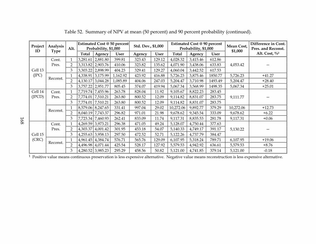
Table 52. Summary of NPV at mean (50 percent) and 90 percent probability (continued).
Estimated Cost @ 50 percent Probability, $1,000 Std. Dev., $1,000 Estimated Cost @ 90 percent
Probability, $1,000 Project ID
Analysis Type Alt.
Total Agency User Agency User Total Agency User
Mean Cost, $1,000
Difference in Cont. Pres. and Reconst.
Alt. Cost, %1 1 3,281.61 2,881.80 399.81 323.43 129.12 4,028.32 3,415.46 612.86 2 3,313.82 2,903.76 410.06 323.82 135.62 4,071.90 3,438.06 633.83
Cont. Pres.
3 3,303.22 2,898.99 404.23 329.41 129.27 4,060.04 3,442.52 617.53 4,053.42
—
1 4,338.91 3,175.99 1,162.92 423.92 416.88 5,726.23 3,875.46 1850.77 5,726.23 +41.27 2 4,130.17 3,044.28 1,085.89 404.06 247.03 5,204.47 3,710.98 1493.49 5,204.47 +28.40
Cell 13 (JPC)
Reconst.
3 3,757.22 2,951.77 805.45 374.07 419.94 5,067.34 3,568.99 1498.35 5,067.34 +25.01 1 7,719.74 7,455.96 263.78 828.04 11.92 9,105.67 8,822.23 283.45 2 7,774.01 7,510.21 263.80 800.52 12.09 9,114.82 8,831.07 283.75
Cont. Pres.
3 7,774.01 7,510.21 263.80 800.52 12.09 9,114.82 8,831.07 283.75 9,111.77
—
1 8,579.06 8,247.65 331.41 997.04 29.02 10,272.06 9,892.77 379.29 10,272.06 +12.73 2 8,040.19 7,743.37 296.82 971.01 21.98 9,678.62 9,345.54 333.09 9,678.62 +6.22
Cell 14 (JPCD)
Reconst.
3 7,723.34 7,460.93 262.41 833.09 11.74 9,117.31 8,835.53 281.78 9,117.31 +0.06 1 4,269.59 3,973.21 296.38 471.05 49.24 5,128.07 4,750.44 377.63 2 4,303.37 4,001.42 301.95 453.18 54.07 5,140.33 4,749.17 391.17
Cont. Pres.
3 4,255.63 3,958.13 297.50 472.52 52.71 5,122.26 4,737.79 384.47 5,130.22
—
1 4,961.45 4,384.74 576.71 565.76 129.09 6,107.95 5,318.24 789.71 6,107.95 +19.06 2 4,496.98 4,071.44 425.54 528.17 127.92 5,579.53 4,942.92 636.61 5,579.53 +8.76
Cell 15 (CRC)
Reconst.
3 4,280.52 3,985.23 295.29 458.56 50.82 5,121.00 4,741.85 379.14 5,121.00 -0.18 1 Positive value means continuous preservation is less expensive alternative. Negative value means reconstruction is less expensive alternative.
168

169
Figure 74. Agency and user costs (50% probability level) for each iteration for analysis cell 1.
Figure 75. Agency and user costs (50% probability level) for each iteration for analysis cell 2.
0
500
1000
1500
2000
2500
Cont.Preser.
Reconst. Cont.Preser.
Reconst. Cont.Preser.
Reconst.
Iter. 1 Iter. 2 Iter. 3
Cos
t ($)
Agency User
0
500
1000
1500
2000
2500
3000
3500
4000
Cont.Preser.
Reconst. Cont.Preser.
Reconst. Cont.Preser.
Reconst.
Iter. 1 Iter. 2 Iter. 3
Cos
t ($)
Agency User

170
Figure 76. Agency and user costs (50% probability level) for each iteration for analysis cell 3.
Figure 77. Agency and user costs (50% probability level) for each iteration for analysis cell 4.
0
500
1000
1500
2000
2500
Cont.Preser.
Reconst. Cont.Preser.
Reconst. Cont.Preser.
Reconst.
Iter. 1 Iter. 2 Iter. 3
Cos
t ($)
Agency User
0
200
400
600
800
1000
1200
1400
Cont.Preser.
Reconst. Cont.Preser.
Reconst. Cont.Preser.
Reconst.
Iter. 1 Iter. 2 Iter. 3
Cos
t ($)
Agency User

171
Figure 78. Agency and user costs (50% probability level) for each iteration for analysis cell 5.
Figure 79. Agency and user costs (50% probability level) for each iteration for analysis cell 6.
0
500
1000
1500
2000
2500
Cont.Preser.
Reconst. Cont.Preser.
Reconst. Cont.Preser.
Reconst.
Iter. 1 Iter. 2 Iter. 3
Cos
t ($)
Agency User
0
500
1000
1500
2000
2500
3000
3500
4000
4500
Cont.Preser.
Reconst. Cont.Preser.
Reconst. Cont.Preser.
Reconst.
Iter. 1 Iter. 2 Iter. 3
Cos
t ($)
Agency User

172
Figure 80. Agency and user costs (50% probability level) for each iteration for analysis cell 7.
Figure 81. Agency and user costs (50% probability level) for each iteration for analysis cell 8.
0
500
1000
1500
2000
2500
3000
3500
4000
Cont.Preser.
Reconst. Cont.Preser.
Reconst. Cont.Preser.
Reconst.
Iter. 1 Iter. 2 Iter. 3
Cos
t ($)
Agency User
0
500
1000
1500
2000
2500
3000
Cont.Preser.
Reconst. Cont.Preser.
Reconst. Cont.Preser.
Reconst.
Iter. 1 Iter. 2 Iter. 3
Cos
t ($)
Agency User

173
Figure 82. Agency and user costs (50% probability level) for each iteration for analysis cell 9.
Figure 83. Agency and user costs (50% probability level) for each iteration for analysis cell 10.
0
200
400
600
800
1000
1200
1400
1600
Cont.Preser.
Reconst. Cont.Preser.
Reconst. Cont.Preser.
Reconst.
Iter. 1 Iter. 2 Iter. 3
Cos
t ($)
Agency User
0
500
1000
1500
2000
2500
Cont.Preser.
Reconst. Cont.Preser.
Reconst. Cont.Preser.
Reconst.
Iter. 1 Iter. 2 Iter. 3
Cos
t ($)
Agency User

174
Figure 84. Agency and user costs (50% probability level) for each iteration for analysis cell 11.
Figure 85. Agency and user costs (50% probability level) for each iteration for analysis cell 12.
1450
1500
1550
1600
1650
1700
1750
1800
Cont.Preser.
Reconst. Cont.Preser.
Reconst. Cont.Preser.
Reconst.
Iter. 1 Iter. 2 Iter. 3
Cos
t ($)
Agency User
0
1000
2000
3000
4000
5000
6000
Cont.Preser.
Reconst. Cont.Preser.
Reconst. Cont.Preser.
Reconst.
Iter. 1 Iter. 2 Iter. 3
Cos
t ($)
Agency User
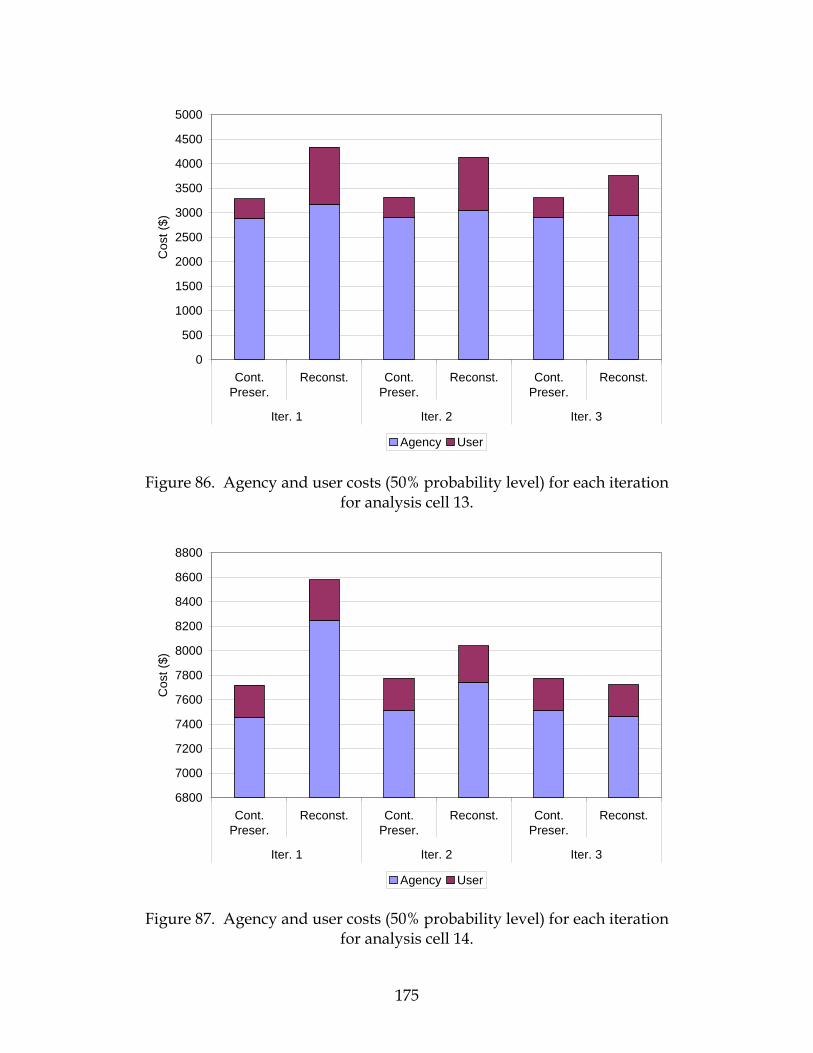
175
Figure 86. Agency and user costs (50% probability level) for each iteration for analysis cell 13.
Figure 87. Agency and user costs (50% probability level) for each iteration for analysis cell 14.
0
500
1000
1500
2000
2500
3000
3500
4000
4500
5000
Cont.Preser.
Reconst. Cont.Preser.
Reconst. Cont.Preser.
Reconst.
Iter. 1 Iter. 2 Iter. 3
Cos
t ($)
Agency User
6800
7000
7200
7400
7600
7800
8000
8200
8400
8600
8800
Cont.Preser.
Reconst. Cont.Preser.
Reconst. Cont.Preser.
Reconst.
Iter. 1 Iter. 2 Iter. 3
Cos
t ($)
Agency User

176
Figure 88. Agency and user costs (50% probability level) for each iteration for analysis cell 15.
Figure 89. Effect of discount rate on cost difference between continuous preservation and reconstruction alternatives.
0
1000
2000
3000
4000
5000
6000
Cont.Preser.
Reconst. Cont.Preser.
Reconst. Cont.Preser.
Reconst.
Iter. 1 Iter. 2 Iter. 3
Cos
t ($)
Agency User
-5
0
5
10
15
20
25
30
35
40
0 4 8 0 4 8
Cell 6 Cell 12Discount Rate, %
Perc
ent D
iffer
ence
(CP
vs R
econ
st)
Iter 1 Iter 2 Iter 3
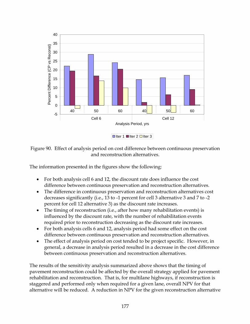
177
Figure 90. Effect of analysis period on cost difference between continuous preservation
and reconstruction alternatives. The information presented in the figures show the following:
• For both analysis cell 6 and 12, the discount rate does influence the cost difference between continuous preservation and reconstruction alternatives.
• The difference in continuous preservation and reconstruction alternatives cost decreases significantly (i.e., 13 to -1 percent for cell 3 alternative 3 and 7 to -2 percent for cell 12 alternative 3) as the discount rate increases.
• The timing of reconstruction (i.e., after how many rehabilitation events) is influenced by the discount rate, with the number of rehabilitation events required prior to reconstruction decreasing as the discount rate increases.
• For both analysis cells 6 and 12, analysis period had some effect on the cost difference between continuous preservation and reconstruction alternatives.
• The effect of analysis period on cost tended to be project specific. However, in general, a decrease in analysis period resulted in a decrease in the cost difference between continuous preservation and reconstruction alternatives.
The results of the sensitivity analysis summarized above shows that the timing of pavement reconstruction could be affected by the overall strategy applied for pavement rehabilitation and reconstruction. That is, for multilane highways, if reconstruction is staggered and performed only when required for a given lane, overall NPV for that alternative will be reduced. A reduction in NPV for the given reconstruction alternative
-5
0
5
10
15
20
25
30
35
40
40 50 60 40 50 60
Cell 6 Cell 12Analysis Period, yrs
Per
cent
Diff
eren
ce (C
P v
s R
econ
st)
Iter 1 Iter 2 Iter 3
178
would result in a forward shift in the timing of reconstruction or a reduction in the number of rehabilitation required prior to reconstruction.
Summary Transportation agencies responsible for providing and maintaining highways and other related infrastructure are always faced with budgetary constraints. Such constraints typically lead to an implementation of cost-cutting measures leading to a haphazard implementation of developmental plans not in the interest of the user public. To avoid this situation, ADOT initiated this study to evaluate in-service pavement design, performance, maintenance and rehabilitation, and cost data to determine the cost-effectiveness of commonly applied pavement maintenance, rehabilitation, and reconstruction strategies. The specific goal was to determine the optimum timing of reconstruction after initial construction (i.e., at what point after initial construction and subjecting a pavement to typical M&R strategies will reconstruction be a more cost-effective solution?). The answer to this question is very important since the trade-off between the cost of continuous preservation activities and reconstruction are important to all highway agencies. All the main elements of highway cost, namely initial capital cost, future maintenance cost, future rehabilitation cost, reconstruction cost, salvage cost at the end of the analysis period, and user cost (traffic delay cost and so on), were considered in the LCCA that was conducted in this study. Results have been presented throughout this chapter. As per the goal of this study, table 52 gives a summary of the mean cost of pursuing the continuous preservation strategy along with three alternate reconstruction strategies. The reconstruction strategies were typically a combination of minor and major rehabilitation activities at different intensities and frequency prior to reconstruction. The alternate reconstruction strategies can be summarized as follows:
• Alternative 1—Reconstruction immediately after initial construction and a minor rehabilitation activity.
• Alternative 2—Reconstruction after both a minor and major rehabilitation activity.
• Alternative 3—Reconstruction after a minor and two major rehabilitation activities.
Detailed descriptions of all the activities within these alternative strategies have been presented and described in chapter 6. To fulfill the goals of this study, a comparison of NPV of each alternative reconstruction strategy was done with the continuous preservation strategy to determine when

179
reconstruction was becomes a more cost-effective strategy in a pavement’s life. The general trend observed for all the 15 cells analyzed showed that in all cases there was a decrease in NPV as the number of rehabilitation activities prior to reconstruction increased. Specifically, the following was observed:
• Nine of the 15 cells analyzed (60 percent) reported a NPV for reconstruction (alternative 3), less than 3 percent that estimated for continuous preservation. Three of the 15 cell reported NPV for reconstruction (alternative 3), less than that estimated for continuous preservation.
• Two of the 15 cells analyzed, reported a NPV for reconstruction (alternative 3), between 3 to 10 percent of the continuous preservation NPV.
• The remaining 4 cells analyzed, reported a NPV for reconstruction (alternative 3), greater than 10 percent of the continuous preservation NPV.
Figure 91 shows the decline in NPV for as the number of rehabilitation events prior to reconstruction (alternative 1 through alternative 3) increases. The information presented in the plot also shows that mean percentage change in NPV dropped significantly from 25.63 percent for reconstruction alternative 1 to 6.9 percent for rehabilitation alternative 3. With this trend it is reasonable to conclude that reconstruction becomes a feasible cost-effective option only after a minor and 2 major rehabilitation events have been performed.

Figure 91. Percent change in NPV between continuous preservation and reconstruction for all analysis cells (alternatives 1 through 3).
-5
0
5
10
15
20
25
30
35
40
45
Cel
l 1
Cel
l 2
Cel
l 3
Cel
l 4
Cel
l 5
Cel
l 6
Cel
l 7
Cel
l 8
Cel
l 9
Cel
l 10
Cel
l 11
Cel
l 12
Cel
l 13
Cel
l 14
Cel
l 15
Per
cent
Diff
eren
ce
Difference b/n CP and Alt 1 Difference b/n CP and Alt 2 Difference b/n CP and Alt 3
180

181
CHAPTER 8. CONCLUSIONS AND RECOMMENDATIONS This study examined the performance and costs of asphalt and concrete pavements used on Arizona highways. Both the initial pavement structure type and the series of M&R treatments applied to each structure type over a long time period were evaluated in an effort to determine the cost-effectiveness of the continuous pavement preservation design strategy, as compared to reconstruction. The pavement types considered in the investigation included conventional asphalt concrete (CAC), deep-strength AC (DSAC), full-depth AC (FDAC), non-doweled jointed plain concrete (JPC), doweled JPC (JPCD), and continuously reinforced concrete (CRC) pavement. Hundreds of M&R treatment types applied to these pavement structures were also considered, but under several broad categories defined by (a) depth of removal (i.e., milling) of existing pavement, (b) treatment application thickness, and (c) type of asphalt mixture used in the treatment. Pavement life and M&R treatment performance for both asphalt and concrete pavements were evaluated using survival analysis techniques, supplemented by mechanistic–empirical (M–E) performance analysis. The evaluations covered 15 different scenarios defined by key variables of interest and the availability of historical pavement data. These 15 scenarios included the following:
• CAC Pavement Interstate highways in hot-dry and moderate climates. Non-Interstate highways in hot-dry, moderate, and cool-wet climates.
• DSAC and FDAC Pavement Interstate highways in hot-dry, moderate, and cool-wet climates. Non-Interstate highways in hot-dry, moderate, and cool-wet climates.
• JPC Pavement All highways in hot-dry and cool-wet climates.
• JPCD Pavement All highways in hot-dry climate.
• CRC Pavement All highways in hot-dry climate.
Unit costs of initial construction and M&R pay items were analyzed to develop best estimates for use in the LCCA process. Three sources of data were utilized in this analysis—the 1999 Construction Costs report, the 2002 Asphalt Rubber Projects report, and the 1999 Engineer’s Estimate.

182
Also investigated in the study were user cost practices. Both user cost components and user cost models were examined to determine the practices most suitable for use in the LCCA process. Using the results the various pavement performance analyses, pay item unit costs analyses, and user cost practices evaluation, a comprehensive set of comparative LCCAs were performed. For each of the 15 scenarios described above, a representative section of highway was chosen to serve as a design project, for which the life-cycle costs of continuous preservation and reconstruction approaches could be determined and compared. Customized life-cycle models were developed for each of the following four alternatives for each project:
• Continuous preservation (i.e., continuous stream of rehabilitation treatments). • Reconstruction with no prior rehabilitation treatments. • Reconstruction with one prior rehabilitation treatment. • Reconstruction with two prior rehabilitation treatments.
The established models, along with the best estimates of unit costs and work zone-related user cost inputs, were then entered into the FHWA probabilistic LCCA spreadsheet program, RealCost, whereupon life-cycle costs were computed using a 60-year analysis period and 4 percent discount rate. Sensitivity analysis was performed by computing life-cycle costs for a couple projects using variations of the discount rate (0, 4, and 8) and analysis period (40, 50, and 60 years). CONCLUSIONS Based on the results of the various analyses performed in this study, the following conclusions are drawn: Initial Pavement Service Life
• On average, throughout the entire State of Arizona, CAC pavements on Interstate routes in the hot-dry and moderate climates have lasted 15 to 18 years (and carried 15 to 20 million trucks) without significant rehabilitation (defined as receiving a 2-in or greater AC overlay [with or without milling]). On Non-Interstate routes, an average life of between 15 and 27 years (carrying 5 to 7 million trucks) has occurred, with the lower end being most representative of life in the cool-wet environment.
• On average, DSAC/FDAC pavements on Interstate routes have lasted 13 to 19 years (and carried 13 to 20 million trucks) without the need for significant rehabilitation. On Non-Interstate routes, an average life between 23 and 27 years (4 to 12 million trucks) was determined.
• JPC (non-doweled) pavements, mostly 11 to 13 in thick and located on freeways in the hot-dry climate can be expected to last about 31 years (and carry 67 million
183
trucks), on average, before the need for significant rehabilitation. On average, 8- to 9-in thick JPC (non-doweled) pavements located on freeways in the cool-wet climate have lasted 18 to 20 years (and carried 9 to 11 million trucks).
• Due to no failures, a formal survival analysis of JPCD pavements could not be conducted. However, based on the existing lives and traffic of JPCD pavements and a mechanistic-based performance analysis, 10- to 13-in JPCD pavements located on freeways in the hot-dry climate can be expected to last at least 20 years (and carry at least 100 million trucks) before significant rehabilitation is needed.
• Due to no failures, a formal survival analysis of CRC pavements could not be conducted. However, based on the existing lives and traffic of CRC pavements and a mechanistic-based performance analysis, 9-in CRC pavements located on freeways in the hot-dry climate can be expected to last at least 30 years (and carry at least 25 million trucks) before significant rehabilitation is needed.
M&R Treatment Performance
• The predominant rehabilitation treatments for asphalt pavements in Arizona have been thin conventional overlays (R1), shallow removal and thin overlays (R3), and shallow removal and thick overlays (R4). On Interstate pavements, many deep removal and thick overlay treatments (R6) have also been applied. Although the average lives of these treatments on Interstate routes have been fairly similar (12 to 16 years), the levels of truck traffic have generally corresponded to the scope/size (mill depth and overlay thickness) of the treatment (e.g., 11 to 18 million trucks for R1 treatment, 29 to 36 million trucks for R6 treatment). On Non-Interstate pavements, much longer average service lives have been provided by the R1 treatments as compared to the R3 and R4 treatments (20 to 24 years versus 14 to 18 years); however, lower truck traffic levels have been experienced (3 to 6 million trucks versus 5 to 14 million trucks).
• The predominant treatments for concrete pavements in Arizona have been thin conventional overlays (R1) and diamond grinding (R7). Based on limited data, the average lives and truck traffic for these treatments have been 11 to 14 years and 8 to 15 million cumulative trucks for R1 and 11 to 15 years and 37 to 55 million cumulative trucks for R7.
• The effect of asphalt mixture on rehabilitation treatment life is only partly discernable due to insufficient performance data to date. Current results indicate better performance by asphalt rubber mixes compared to conventional asphalt mixes when used with some treatments (thin conventional overlays [R1] on Non-interstate pavements) and worse performance when used with others (shallow removal and thin overlays [R3] placed on Interstate pavements). Moreover, similar or better performance has been experienced by some treatments (R3 on Interstate and Non-Interstate pavements) using recycled asphalt mixes, as compared to conventional asphalt mixes. The performance of treatments using SuperPave asphalt mixes was not evaluated due to the lack of performance data.

184
Climatic Effects • The effect of climate on initial pavement life and rehabilitation treatment
performance was most significant for the cool-wet climatic zone. Although some differences in asphalt pavement performance existed between the hot-dry and moderate climates, substantial reductions in life were consistently observed for pavements in the cool-wet climate. The effect of climate on rigid pavements was not evaluated due to insufficient data.
Construction and M&R Pay Item Unit Costs
• With the exception of various concrete pavement-related pay items, sufficient data were available to develop best estimates of unit costs for use in the LCCAs conducted in this study. All original cost data were inflated to 2003 values and, where appropriate, were reprocessed to filter out the effects of projects having small quantities.
• Generally good agreement was found between the unit cost estimates derived from the three data sources used—the 1999 Construction Costs report, the 2002 Asphalt Rubber Projects report, and the 1999 Pavement Management Cost Estimate.
• For pay items with limited or no cost data, best estimates were developed using all available cost information and engineering judgment.
User Cost Practices
• User cost components that are predominately evaluated by highway agencies are the user delay costs resulting from traffic slowdowns and disruption that occur during construction and M&R operations. A secondary cost that is evaluated is the increased vehicle operating cost (VOC) that results from decreased pavement smoothness.
• The process favored for evaluation of user delay costs is the procedure outlined in the FHWA Interim Technical Bulletin on Life Cycle Cost Analysis in Pavement Design (Walls and Smith, 1998).
Life-Cycle Costs
• For all 15 projects investigated using a 4 percent discount rate and 60-year analysis period, a consistent reduction in total life-cycle costs was observed corresponding to an increase (from 0 to 2) in the number of rehabilitations between initial construction and the first reconstruction. Thus, there is economic value in performing at least one or two sequential rehabilitation treatments prior to reconstruction.
• For 9 of the 15 scenarios investigated, the total life-cycle costs associated with the third reconstruction alternative (two rehabilitations prior to reconstruction) were within 3 percent (sometimes higher, sometimes lower) of the total life-cycle costs of the continuous preservation strategy. Hence, based on a 4 percent discount rate and 60-year analysis period, the break-even point between the continuous preservation strategy and the reconstruction strategy typically occurs after two to

185
three cycles of rehabilitation (i.e., reconstruction preceded by two to three sequential rehabilitation treatments). The exact timing of the break-even point, in terms of years, is largely dependent upon the pavement design and the conditions in which it is used.
• An increase in the discount rate results in a corresponding decrease in the life-cycle cost differences between the continuous preservation and reconstruction alternatives. Thus, use of a higher discount rate favors a reduction in the number of rehabilitation events prior to reconstruction. Conversely, a lower discount rate favors a continuous preservation strategy.
• A decrease in analysis period from 60 to 40 years results in a decrease in the life-cycle cost differences between continuous preservation and reconstruction. The rate of decrease is case specific.
RECOMMENDATIONS The following recommendations are offered as related to the pavement strategies currently used by ADOT:
• Pavement survival analyses should be routinely (perhaps biennially) performed to develop more complete and accurate estimates of initial pavement life and rehabilitation performance. Specifically, an improved database with few errors is greatly needed for all pavements of interest and better forecasting is needed for a variety of designs/materials: SuperPave mixes, JPCD pavements (the current Arizona design), concrete pavement rehabilitation treatments, and asphalt pavement rehabilitation treatments utilizing different asphalt mixtures.
• A comprehensive economic analysis, using reasonably accurate estimates of pavement life and traffic loadings, should be performed for all major pavement projects to determine not only the type of pavement to use, but the optimal timing of reconstruction. For most of the conditions prevailing in Arizona, a reasonable estimate of the optimal timing for reconstruction is after the sequential application of two to three rehabilitation activities.
• The practice of programming pavements for improvement and performing detailed evaluations and testing to determine the best improvement strategy should continue, but the history of the pavement should be reviewed to determine if reconstruction should be considered as an option. If records show that the existing pavement has been rehabilitated at least twice since original construction, then an economic analysis should be performed to determine whether the pavement should undergo another rehabilitation or be reconstructed.
• User costs stemming from the time delay associated with work zones should be evaluated as part of the pavement LCCA. The FHWA process (RealCost) is the preferred method for determining these costs; however, use of the QuickZone

186
user cost program should be considered in cases where urban freeways or areas with detours or complete road closures are being evaluated.
• The evaluation of VOCs resulting from decreased pavement smoothness should be considered in pavement LCCA. Moreover, the use of cost adjustment factors, such as those used by the Minnesota DOT, should be considered, particularly for pavements maintained at a lower serviceability level.
187
REFERENCES Aghazadeh, F., G. Knapp, and T. Ray. 2003. Analysis of User Waiting Costs for Construction Projects on Louisiana’s Interstate Highway System, Report No. FHWA/LA.03/372, Louisiana Transportation Research Center (LTRC), Baton Rouge, Louisiana. Arizona Department of Transportation (ADOT). 1999. “1999 Construction Costs,” Report prepared by ADOT Contracts and Specifications Section, Phoenix, Arizona. ADOT. 2002. “Arizona Asphalt Rubber Projects, 1988-2001,” prepared by ADOT Materials Group Pavement Design Section, Phoenix, Arizona. ADOT. 1999. “Pavement Management Cost Estimate,” Document obtained from ADOT website www.dot.state.az.us. Barnes, G. and P. Langworthy. 2003. “The Per-Mile Costs Of Operating Automobiles And Trucks,” Report MN/RC 2003-19, Minnesota Department of Transportation, Office of Research Services, St. Paul, Minnesota. ERES Consultants Division of Applied Research Associates, Inc. 2003. “Ohio Pavement Selection Process Analysis,” Neutral Third Party Final Report prepared for Ohio Department of Transportation, Columbus, Ohio. Federal Highway Administration (FHWA). 1999. Pavement Preservation: A Road Map for the Future, FHWA-SA-99-015, Forum held October 26-28, 1998 in Kansas City, Kansas. FHWA. 2000. Insights into Pavement Preservation: A Compendium, U.S. Department of Transportation, FHWA, Washington, D.C. FHWA. 2002. Highway Economics Requirement System, State Version Overview, FHWA, Washington, D.C. FHWA. 2004. “RealCost (Version 2.1) Pavement Life-Cycle Cost Analysis,” Office of Asset Management, FHWA, Washington, D.C. Gharaibeh, N.G., M.I. Darter, F. LaTorre, J.W. Vespa, and D.L. Lippert. 1997. “Performance of Original and Resurfaced Pavements on the Illinois Freeway System,” Illinois Cooperative Highway Research Program (ICHRP) Research Report No. 540-1, Illinois Department of Transportation, Springfield, Illinois.
188
Hall, K.T., M.I. Darter, and W.M. Rexroad. 1993. “Performance of Bare and Resurfaced JRCP and CRCP on the Illinois Interstate Highway System: 1991 Update,” Illinois Cooperative Highway Research Program (ICHRP) Research Report No. 532-1, Illinois Department of Transportation, Springfield, Illinois. National Cooperative Highway Research Program (NCHRP). 1995. “Metrication and Enhancement of MicroBENCOST Software Package,” NCHRP Project 7-12(2), NCHRP, Washington, D.C. Rister, B.W. and C. Graves. 2002. “Cost of Construction Delays and Traffic Control for Life-Cycle Cost Analysis of Pavements,” Report KTC-02-07/SPR 197-99 & SPR 218-00-1F, Kentucky Transportation Center, Lexington, Kentucky. Walls III, J. and M.R. Smith. 1998. Life-Cycle Cost Analysis in Pavement Design—Interim Technical Bulletin, Report No. FHWA-SA-98-079, FHWA, Washington, D.C. Way, G. 1983. “Research Pays Off: Arizona DOT Adopts PMS and $ave$ a Bundle,” TRN 107, Arizona DOT, Phoenix, Arizona.

APPENDIX A. PAVEMENT SURVIVAL CURVES


A-1
Figure A-1. Age- and truck traffic-based survival plots for CAC Interstate pavements located in hot-dry climate (analysis cell 1).

A-2
Figure A-2. Age- and truck traffic-based survival plots for CAC Interstate pavements located in moderate climate (analysis cell 2).

A-3
Figure A-3. Age- and truck traffic-based survival plots for CAC Non-Interstate pavements located in hot-dry climate (analysis cell 3).
O Censored data point
O Censored data point
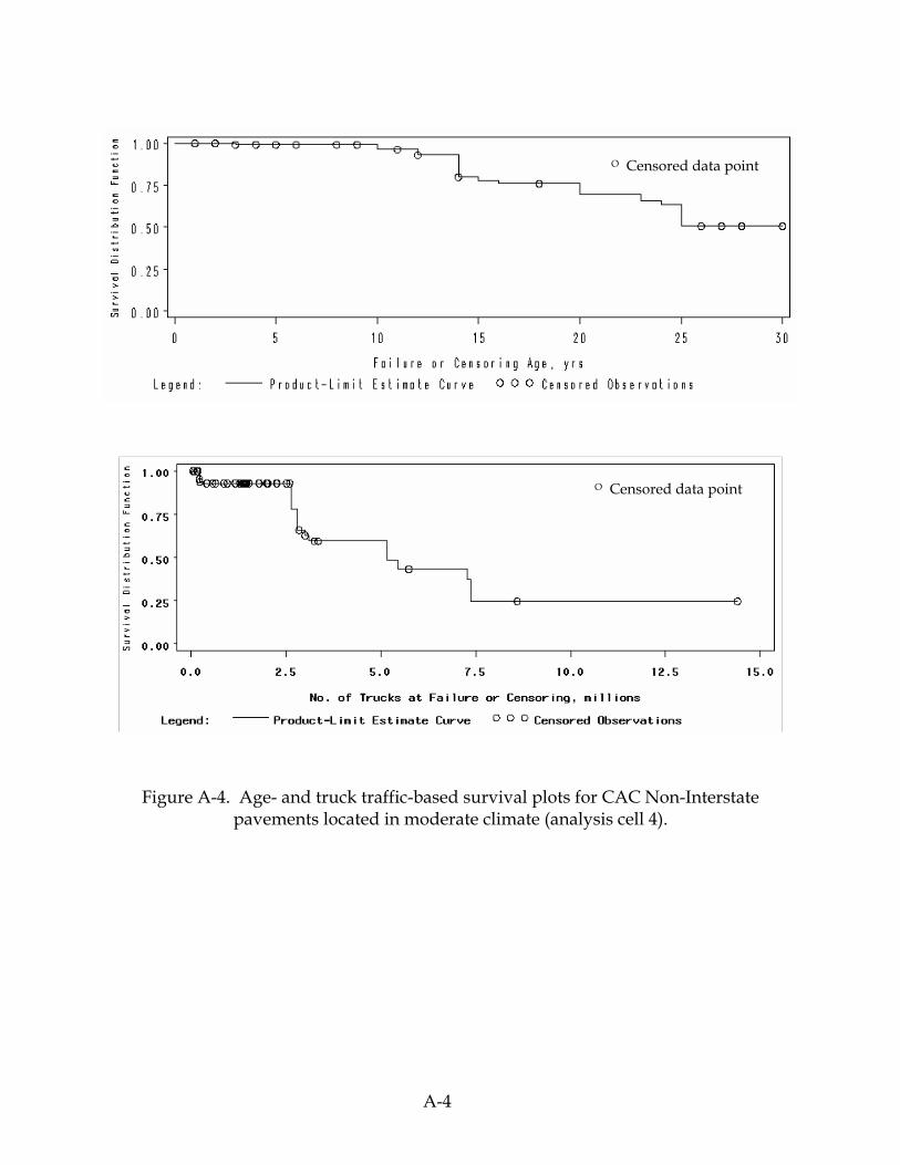
A-4
Figure A-4. Age- and truck traffic-based survival plots for CAC Non-Interstate pavements located in moderate climate (analysis cell 4).
O Censored data point
O Censored data point

A-5
Figure A-5. Age- and truck traffic-based survival plots for CAC Non-Interstate pavements located in cool-wet climate (analysis cell 5).
O Censored data point
O Censored data point

A-6
Figure A-6. Age- and truck traffic-based survival plots for DSAC/FDAC Interstate pavements located in hot-dry climate (analysis cell 6).
O Censored data point
O Censored data point

A-7
Figure A-7. Age- and truck traffic-based survival plots for DSAC/FDAC Interstate pavements located in moderate climate (analysis cell 7).
O Censored data point
O Censored data point

A-8
Figure A-8. Age- and truck traffic-based survival plots for DSAC/FDAC Interstate pavements located in cool-wet climate (analysis cell 8).

A-9
Figure A-9. Age- and truck traffic-based survival plots for DSAC/FDAC Non-Interstate
pavements located in hot-dry climate (analysis cell 9).
O Censored data point
O Censored data point

A-10
Figure A-10. Age- and truck traffic-based survival plots for DSAC/FDAC Non-Interstate pavements located in moderate climate (analysis cell 10).
O Censored data point
O Censored data point
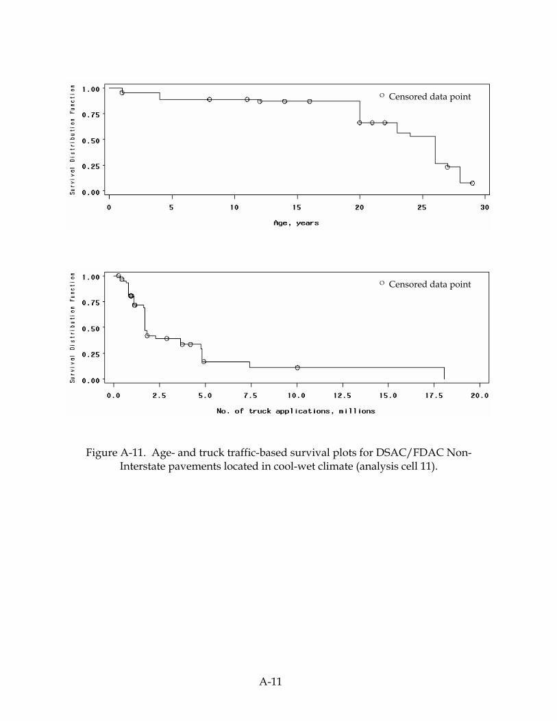
A-11
Figure A-11. Age- and truck traffic-based survival plots for DSAC/FDAC Non-Interstate pavements located in cool-wet climate (analysis cell 11).
O Censored data point
O Censored data point

A-12
Figure A-12. Age- and truck traffic-based survival plots for JPC pavements located in hot-dry climate (analysis cell 12).
O Censored data point
O Censored data point
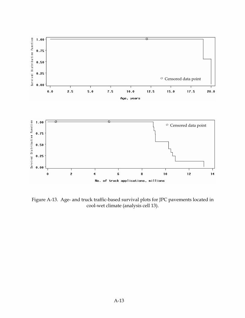
A-13
Figure A-13. Age- and truck traffic-based survival plots for JPC pavements located in cool-wet climate (analysis cell 13).
O Censored data point
O Censored data point

A-14
Figure A-14. Age- and truck traffic-based survival plots for JPCD pavements located in
hot-dry climate (analysis cell 14).
O Censored data point
O Censored data point

A-15
Figure A-15. Age- and truck traffic-based survival plots for CRC pavements located in
hot-dry climate (analysis cell 15).
O Censored data point
O Censored data point

A-16
Figure A-16. Age- and truck traffic-based survival plots for R1A rehabilitation treatments applied to asphalt Interstate pavements located in hot-dry climate.

A-17
Figure A-17. Age- and truck traffic-based survival plots for R1A rehabilitation treatments applied to asphalt Interstate pavements located in moderate climate.

A-18
Figure A-18. Age- and truck traffic-based survival plots for R1A rehabilitation treatments applied to asphalt Interstate pavements located in cool-wet climate.
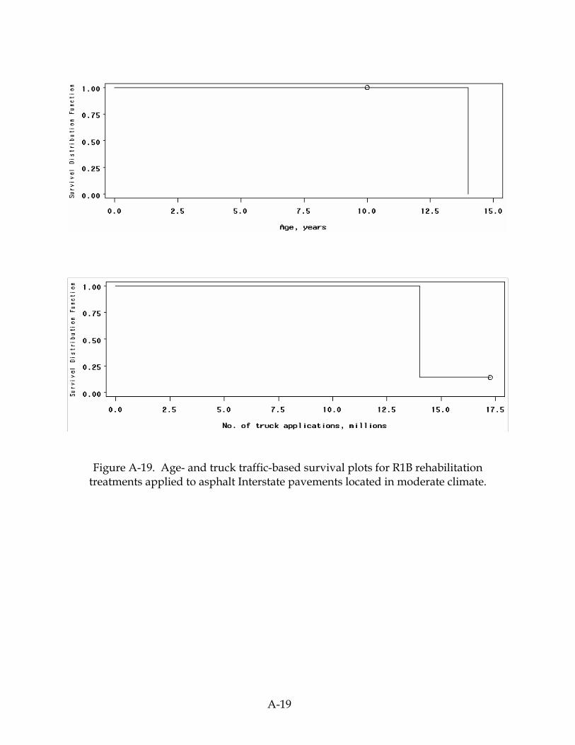
A-19
Figure A-19. Age- and truck traffic-based survival plots for R1B rehabilitation treatments applied to asphalt Interstate pavements located in moderate climate.
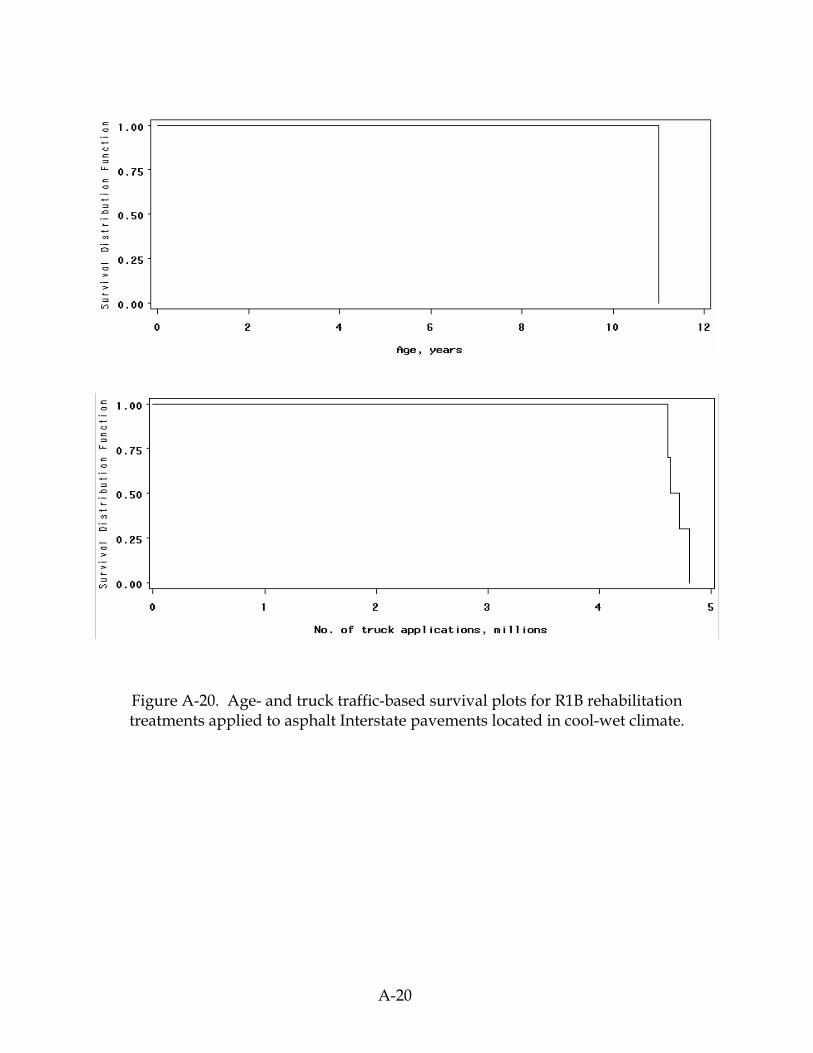
A-20
Figure A-20. Age- and truck traffic-based survival plots for R1B rehabilitation treatments applied to asphalt Interstate pavements located in cool-wet climate.

A-21
Figure A-21. Age- and truck traffic-based survival plots for R2A rehabilitation treatments applied to asphalt Interstate pavements located in hot-dry climate.

A-22
Figure A-22. Age- and truck traffic-based survival plots for R2A rehabilitation treatments applied to asphalt Interstate pavements located in moderate climate.
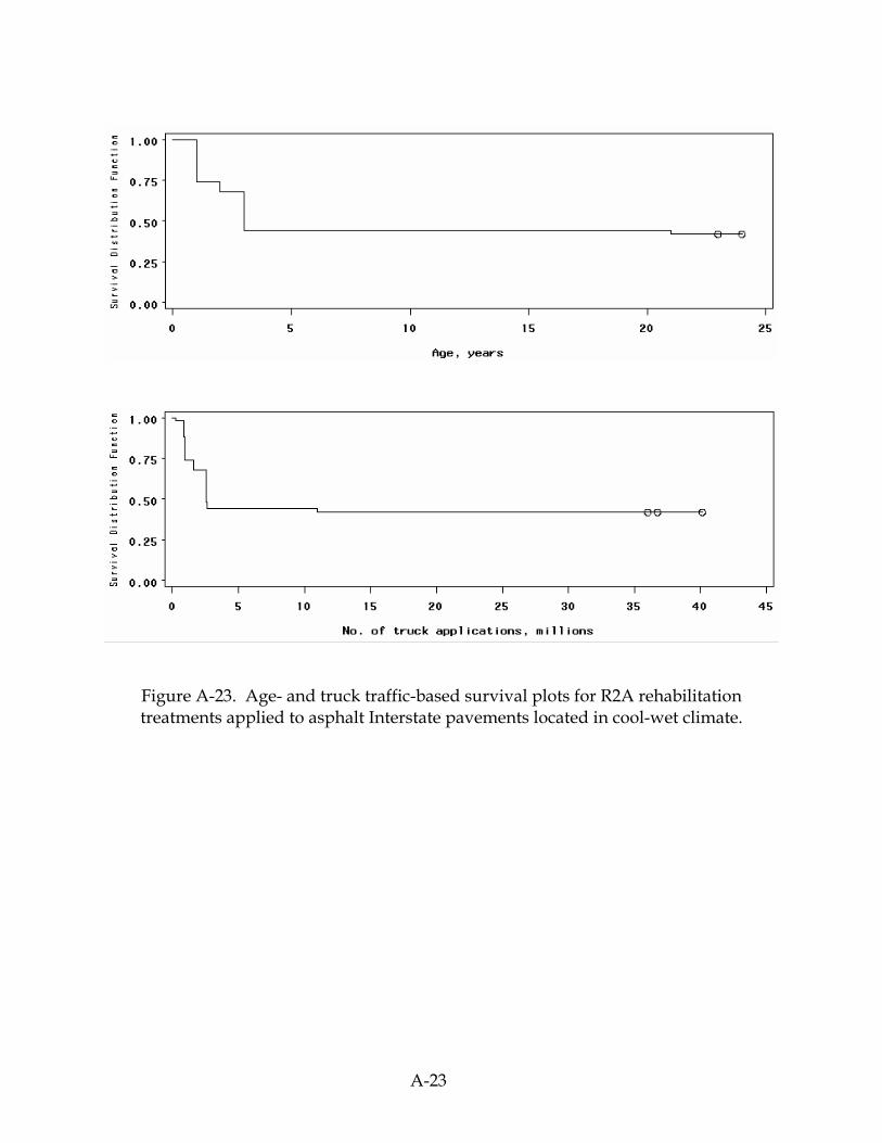
A-23
Figure A-23. Age- and truck traffic-based survival plots for R2A rehabilitation treatments applied to asphalt Interstate pavements located in cool-wet climate.

A-24
Figure A-24. Age- and truck traffic-based survival plots for R3A rehabilitation treatments applied to asphalt Interstate pavements located in hot-dry climate.

A-25
Figure A-25. Age- and truck traffic-based survival plots for R3A rehabilitation treatments applied to asphalt Interstate pavements located in moderate climate.
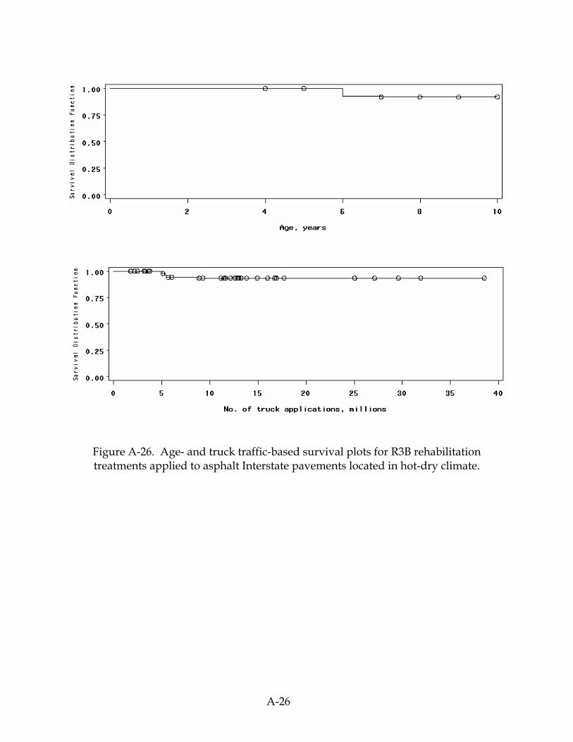
A-26
Figure A-26. Age- and truck traffic-based survival plots for R3B rehabilitation treatments applied to asphalt Interstate pavements located in hot-dry climate.
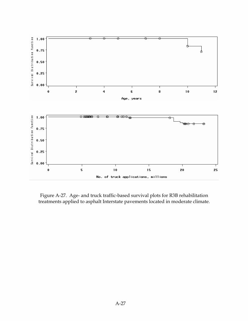
A-27
Figure A-27. Age- and truck traffic-based survival plots for R3B rehabilitation treatments applied to asphalt Interstate pavements located in moderate climate.

A-28
Figure A-28. Age- and truck traffic-based survival plots for R3B rehabilitation treatments applied to asphalt Interstate pavements located in cool-wet climate.

A-29
Figure A-29. Age- and truck traffic-based survival plots for R3C rehabilitation treatments applied to asphalt Interstate pavements located in moderate climate.

A-30
Figure A-30. Age- and truck traffic-based survival plots for R3D rehabilitation treatments applied to asphalt Interstate pavements located in hot-dry climate.
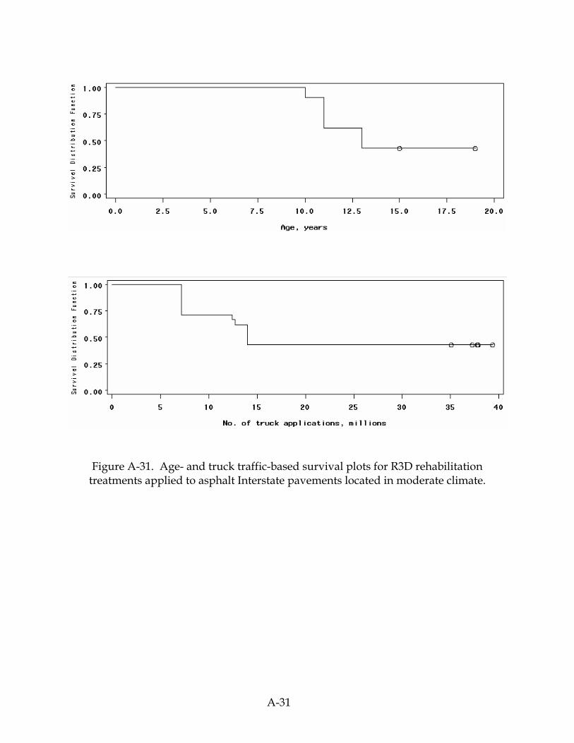
A-31
Figure A-31. Age- and truck traffic-based survival plots for R3D rehabilitation treatments applied to asphalt Interstate pavements located in moderate climate.
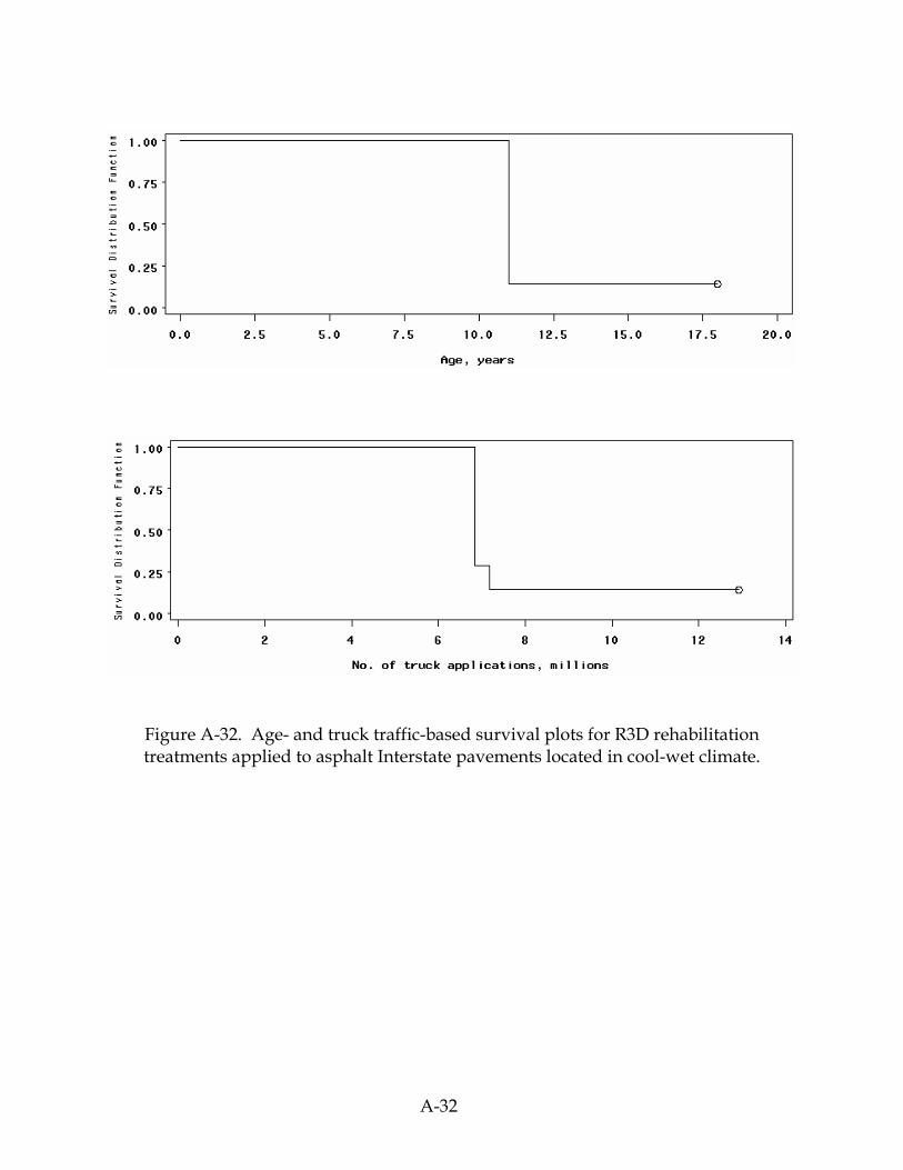
A-32
Figure A-32. Age- and truck traffic-based survival plots for R3D rehabilitation treatments applied to asphalt Interstate pavements located in cool-wet climate.

A-33
Figure A-33. Age- and truck traffic-based survival plots for R4A rehabilitation treatments applied to asphalt Interstate pavements located in hot-dry climate.

A-34
Figure A-34. Age- and truck traffic-based survival plots for R4A rehabilitation treatments applied to asphalt Interstate pavements located in moderate climate.

A-35
Figure A-35. Age- and truck traffic-based survival plots for R4B rehabilitation treatments applied to asphalt Interstate pavements located in hot-dry climate.

A-36
Figure A-36. Age- and truck traffic-based survival plots for R4B rehabilitation treatments applied to asphalt Interstate pavements located in moderate climate.
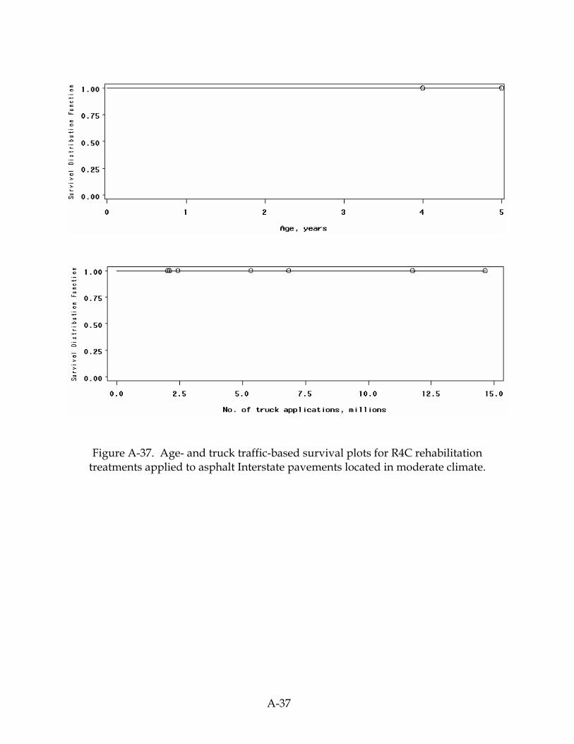
A-37
Figure A-37. Age- and truck traffic-based survival plots for R4C rehabilitation treatments applied to asphalt Interstate pavements located in moderate climate.

A-38
Figure A-38. Age- and truck traffic-based survival plots for R4D rehabilitation treatments applied to asphalt Interstate pavements located in hot-dry climate.

A-39
Figure A-39. Age- and truck traffic-based survival plots for R4D rehabilitation treatments applied to asphalt Interstate pavements located in moderate climate.
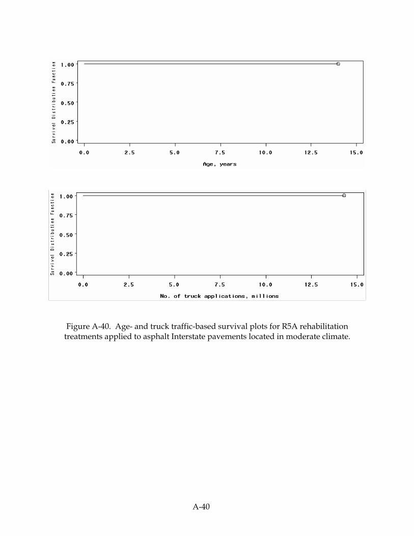
A-40
Figure A-40. Age- and truck traffic-based survival plots for R5A rehabilitation treatments applied to asphalt Interstate pavements located in moderate climate.

A-41
Figure A-41. Age- and truck traffic-based survival plots for R6A rehabilitation treatments applied to asphalt Interstate pavements located in hot-dry climate.
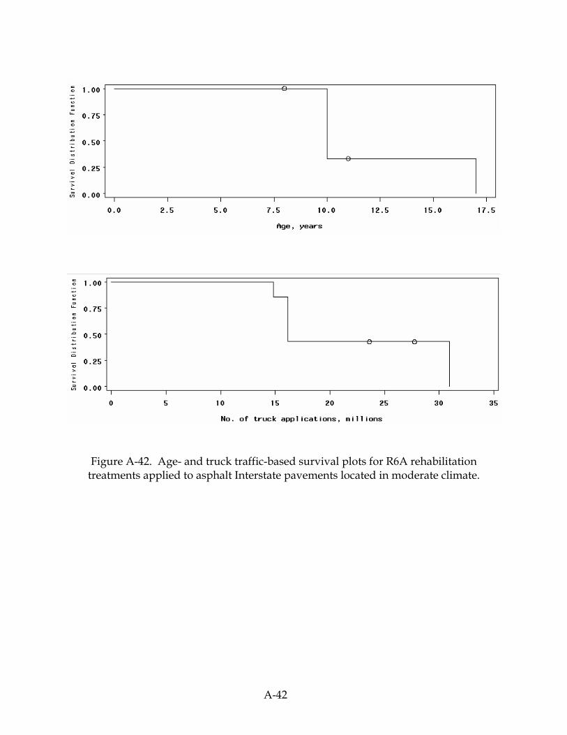
A-42
Figure A-42. Age- and truck traffic-based survival plots for R6A rehabilitation treatments applied to asphalt Interstate pavements located in moderate climate.

A-43
Figure A-43. Age- and truck traffic-based survival plots for R6B rehabilitation treatments applied to asphalt Interstate pavements located in hot-dry climate.

A-44
Figure A-44. Age- and truck traffic-based survival plots for R6B rehabilitation treatments applied to asphalt Interstate pavements located in moderate climate.
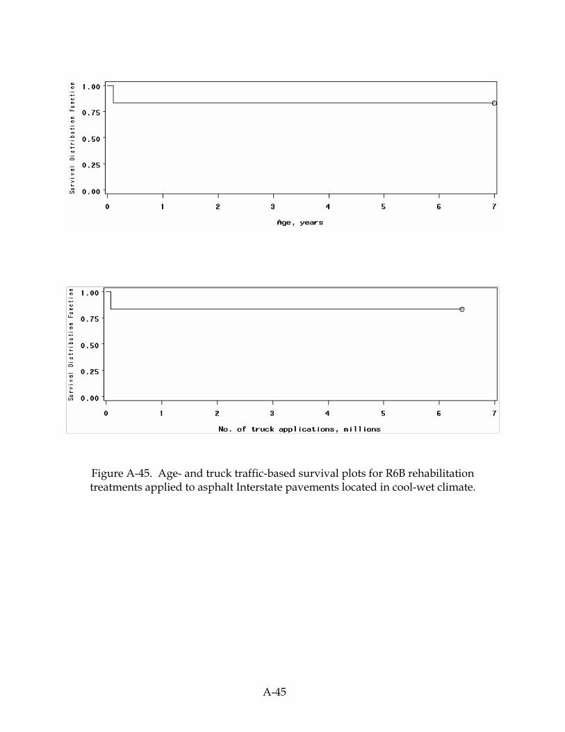
A-45
Figure A-45. Age- and truck traffic-based survival plots for R6B rehabilitation treatments applied to asphalt Interstate pavements located in cool-wet climate.

A-46
Figure A-46. Age- and truck traffic-based survival plots for R6C rehabilitation treatments applied to asphalt Interstate pavements located in hot-dry climate.

A-47
Figure A-47. Age- and truck traffic-based survival plots for R6C rehabilitation treatments applied to asphalt Interstate pavements located in moderate climate.

A-48
Figure A-48. Age- and truck traffic-based survival plots for R6D rehabilitation treatments applied to asphalt Interstate pavements located in hot-dry climate.

A-49
Figure A-49. Age- and truck traffic-based survival plots for R6D rehabilitation treatments applied to asphalt Interstate pavements located in moderate climate.
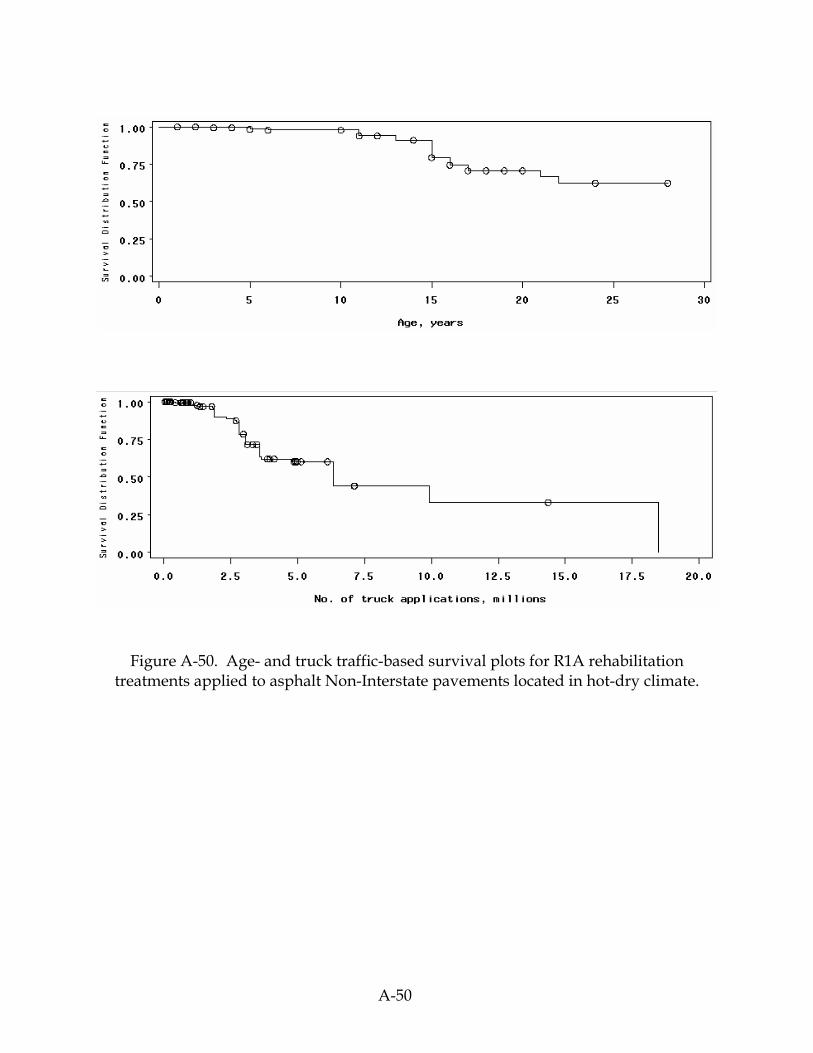
A-50
Figure A-50. Age- and truck traffic-based survival plots for R1A rehabilitation treatments applied to asphalt Non-Interstate pavements located in hot-dry climate.

A-51
Figure A-51. Age- and truck traffic-based survival plots for R1A rehabilitation treatments applied to asphalt Non-Interstate pavements located in moderate climate.

A-52
Figure A-52. Age- and truck traffic-based survival plots for R1A rehabilitation treatments applied to asphalt Non-Interstate pavements located in cool-wet climate.

A-53
Figure A-53. Age- and truck traffic-based survival plots for R1B rehabilitation treatments applied to asphalt Non-Interstate pavements located in hot-dry climate.

A-54
Figure A-54. Age- and truck traffic-based survival plots for R1B rehabilitation treatments applied to asphalt Non-Interstate pavements located in moderate climate.

A-55
Figure A-55. Age- and truck traffic-based survival plots for R1B rehabilitation treatments applied to asphalt Non-Interstate pavements located in cool-wet climate.

A-56
Figure A-56. Age- and truck traffic-based survival plots for R2A rehabilitation treatments applied to asphalt Non-Interstate pavements located in hot-dry climate.

A-57
Figure A-57. Age- and truck traffic-based survival plots for R2A rehabilitation treatments applied to asphalt Non-Interstate pavements located in moderate climate.

A-58
Figure A-58. Age- and truck traffic-based survival plots for R2A rehabilitation treatments applied to asphalt Non-Interstate pavements located in cool-wet climate.

A-59
Figure A-59. Age- and truck traffic-based survival plots for R3A rehabilitation treatments applied to asphalt Non-Interstate pavements located in hot-dry climate.
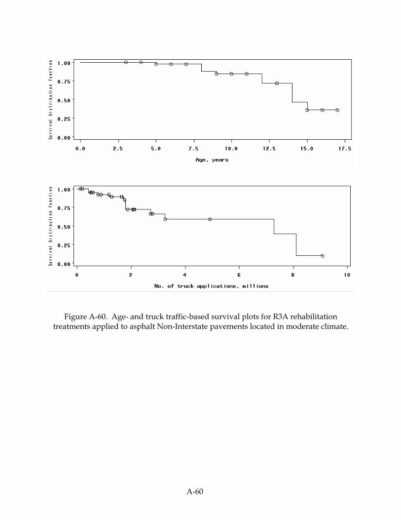
A-60
Figure A-60. Age- and truck traffic-based survival plots for R3A rehabilitation treatments applied to asphalt Non-Interstate pavements located in moderate climate.
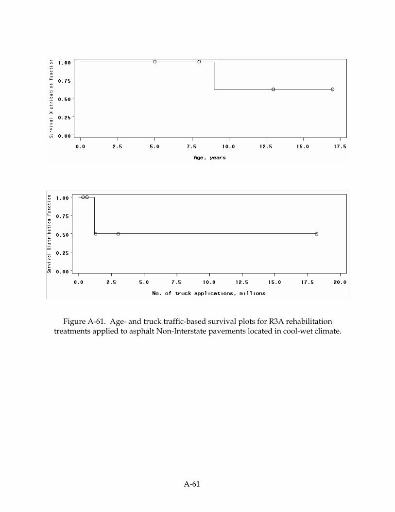
A-61
Figure A-61. Age- and truck traffic-based survival plots for R3A rehabilitation treatments applied to asphalt Non-Interstate pavements located in cool-wet climate.

A-62
Figure A-62. Age- and truck traffic-based survival plots for R3B rehabilitation treatments applied to asphalt Non-Interstate pavements located in hot-dry climate.

A-63
Figure A-63. Age- and truck traffic-based survival plots for R3B rehabilitation treatments applied to asphalt Non-Interstate pavements located in moderate climate.

A-64
Figure A-64. Age- and truck traffic-based survival plots for R3B rehabilitation treatments applied to asphalt Non-Interstate pavements located in cool-wet climate.

A-65
Figure A-65. Age- and truck traffic-based survival plots for R3C rehabilitation treatments applied to asphalt Non-Interstate pavements located in hot-dry climate.

A-66
Figure A-66. Age- and truck traffic-based survival plots for R3C rehabilitation treatments applied to asphalt Non-Interstate pavements located in moderate climate.
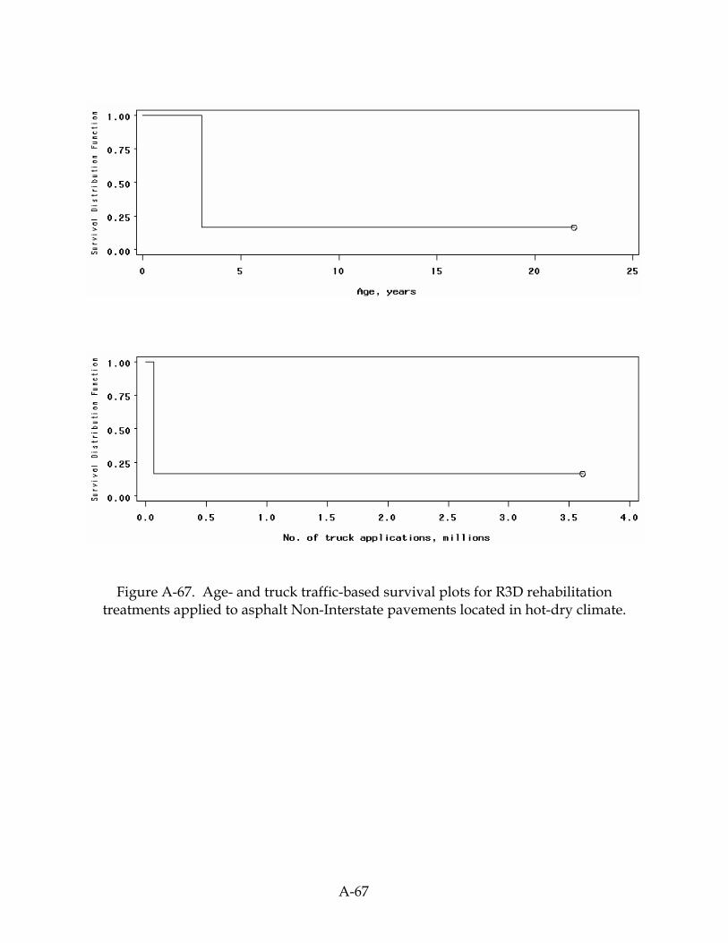
A-67
Figure A-67. Age- and truck traffic-based survival plots for R3D rehabilitation treatments applied to asphalt Non-Interstate pavements located in hot-dry climate.

A-68
Figure A-68. Age- and truck traffic-based survival plots for R3D rehabilitation treatments applied to asphalt Non-Interstate pavements located in moderate climate.

A-69
Figure A-69. Age- and truck traffic-based survival plots for R3D rehabilitation treatments applied to asphalt Non-Interstate pavements located in cool-wet climate.
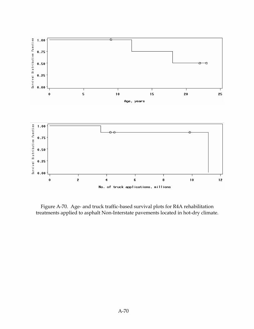
A-70
Figure A-70. Age- and truck traffic-based survival plots for R4A rehabilitation treatments applied to asphalt Non-Interstate pavements located in hot-dry climate.

A-71
Figure A-71. Age- and truck traffic-based survival plots for R4A rehabilitation treatments applied to asphalt Non-Interstate pavements located in moderate climate.

A-72
Figure A-72. Age- and truck traffic-based survival plots for R4A rehabilitation treatments applied to asphalt Non-Interstate pavements located in cool-wet climate.

A-73
Figure A-73. Age- and truck traffic-based survival plots for R4B rehabilitation treatments applied to asphalt Non-Interstate pavements located in hot-dry climate.
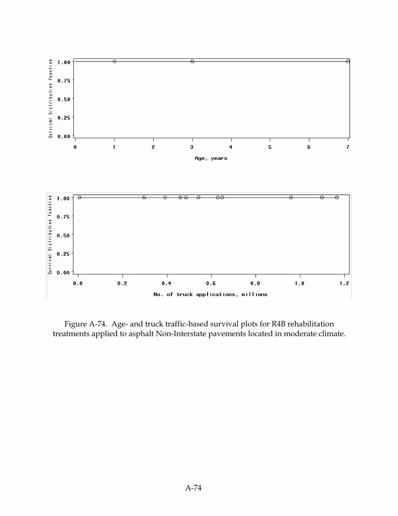
A-74
Figure A-74. Age- and truck traffic-based survival plots for R4B rehabilitation treatments applied to asphalt Non-Interstate pavements located in moderate climate.

A-75
Figure A-75. Age- and truck traffic-based survival plots for R4B rehabilitation treatments applied to asphalt Non-Interstate pavements located in cool-wet climate.
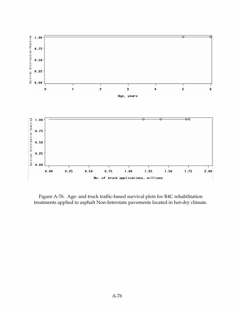
A-76
Figure A-76. Age- and truck traffic-based survival plots for R4C rehabilitation treatments applied to asphalt Non-Interstate pavements located in hot-dry climate.
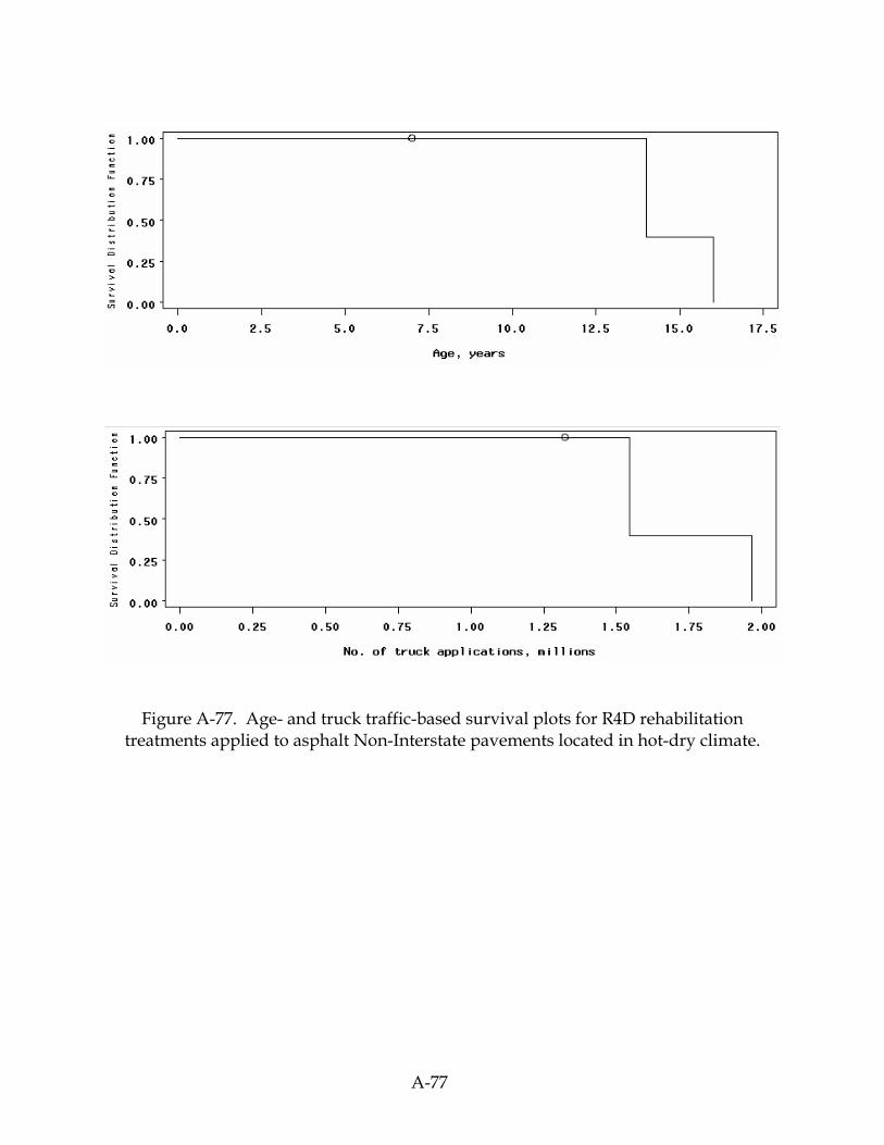
A-77
Figure A-77. Age- and truck traffic-based survival plots for R4D rehabilitation treatments applied to asphalt Non-Interstate pavements located in hot-dry climate.

A-78
Figure A-78. Age- and truck traffic-based survival plots for R4D rehabilitation treatments applied to asphalt Non-Interstate pavements located in moderate climate.

A-79
Figure A-79. Age- and truck traffic-based survival plots for R4D rehabilitation treatments applied to asphalt Non-Interstate pavements located in cool-wet climate.

A-80
Figure A-80. Age- and truck traffic-based survival plots for R6A rehabilitation treatments applied to asphalt Non-Interstate pavements located in hot-dry climate.

A-81
Figure A-81. Age- and truck traffic-based survival plots for R6A rehabilitation treatments applied to asphalt Non-Interstate pavements located in moderate climate.
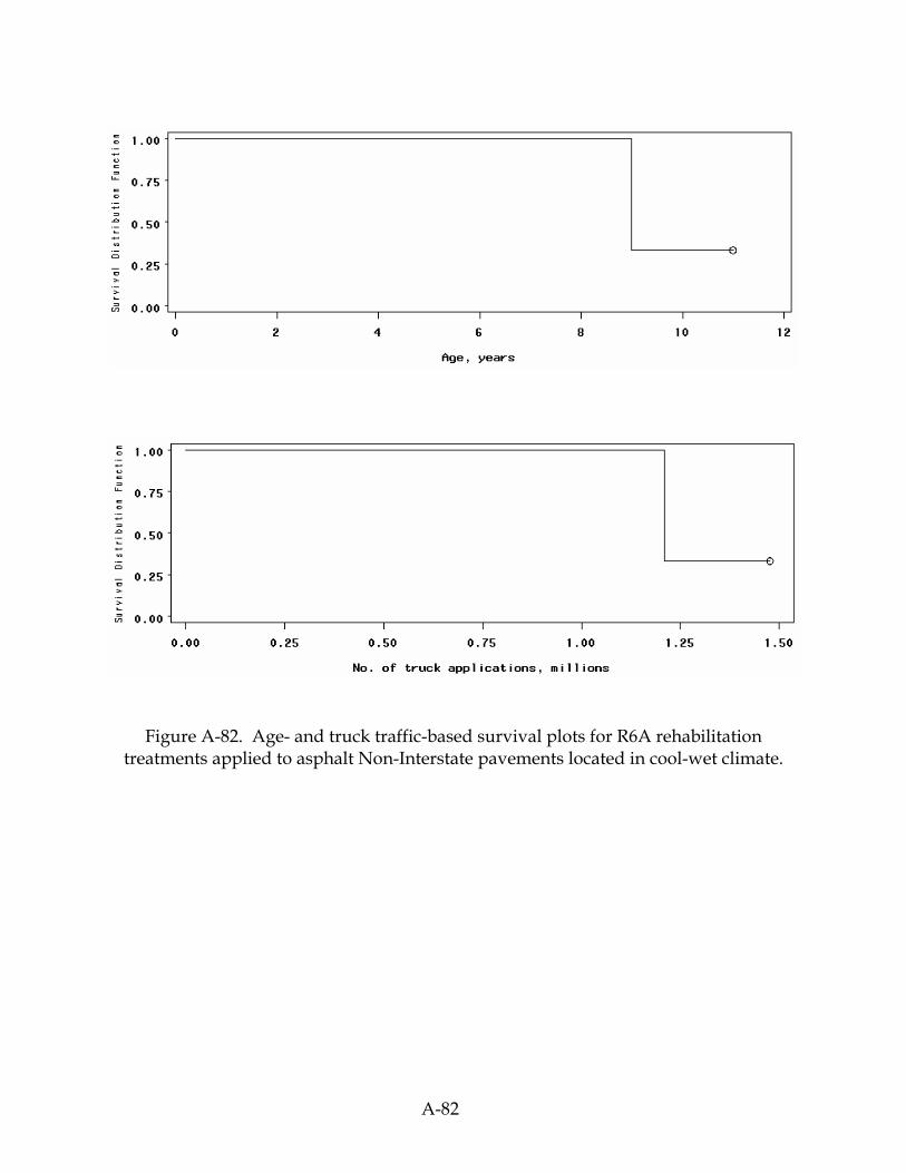
A-82
Figure A-82. Age- and truck traffic-based survival plots for R6A rehabilitation treatments applied to asphalt Non-Interstate pavements located in cool-wet climate.

A-83
Figure A-83. Age- and truck traffic-based survival plots for R1A rehabilitation treatments applied to JPC pavements located in moderate climate.
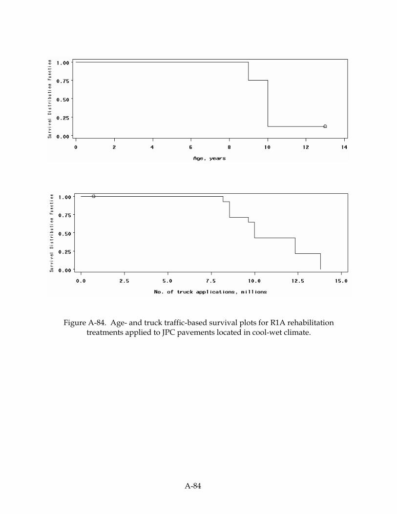
A-84
Figure A-84. Age- and truck traffic-based survival plots for R1A rehabilitation treatments applied to JPC pavements located in cool-wet climate.
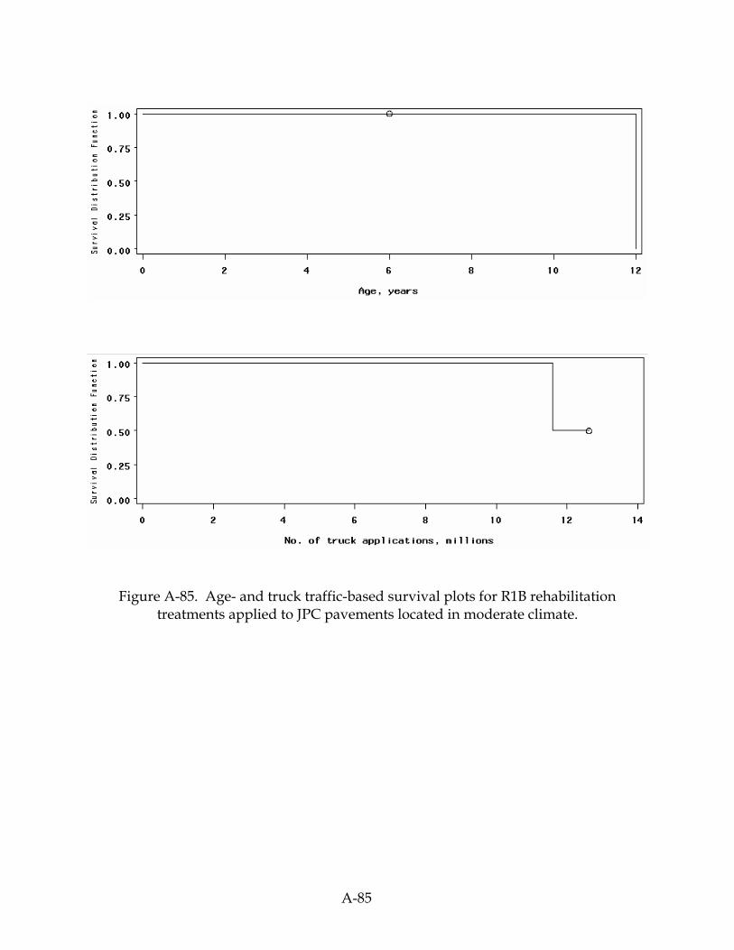
A-85
Figure A-85. Age- and truck traffic-based survival plots for R1B rehabilitation treatments applied to JPC pavements located in moderate climate.
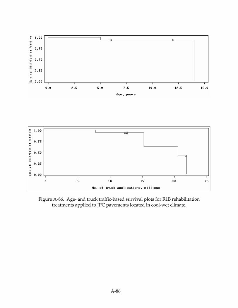
A-86
Figure A-86. Age- and truck traffic-based survival plots for R1B rehabilitation treatments applied to JPC pavements located in cool-wet climate.

A-87
Figure A-87. Age- and truck traffic-based survival plots for R2B rehabilitation treatments applied to JPC pavements located in moderate climate.

A-88
Figure A-88. Age- and truck traffic-based survival plots for R2B rehabilitation treatments applied to JPC pavements located in cool-wet climate.

A-89
Figure A-89. Age- and truck traffic-based survival plots for R3B rehabilitation treatments applied to JPC pavements located in moderate climate.

A-90
Figure A-90. Age- and truck traffic-based survival plots for R3B rehabilitation treatments applied to JPC pavements located in cool-wet climate.
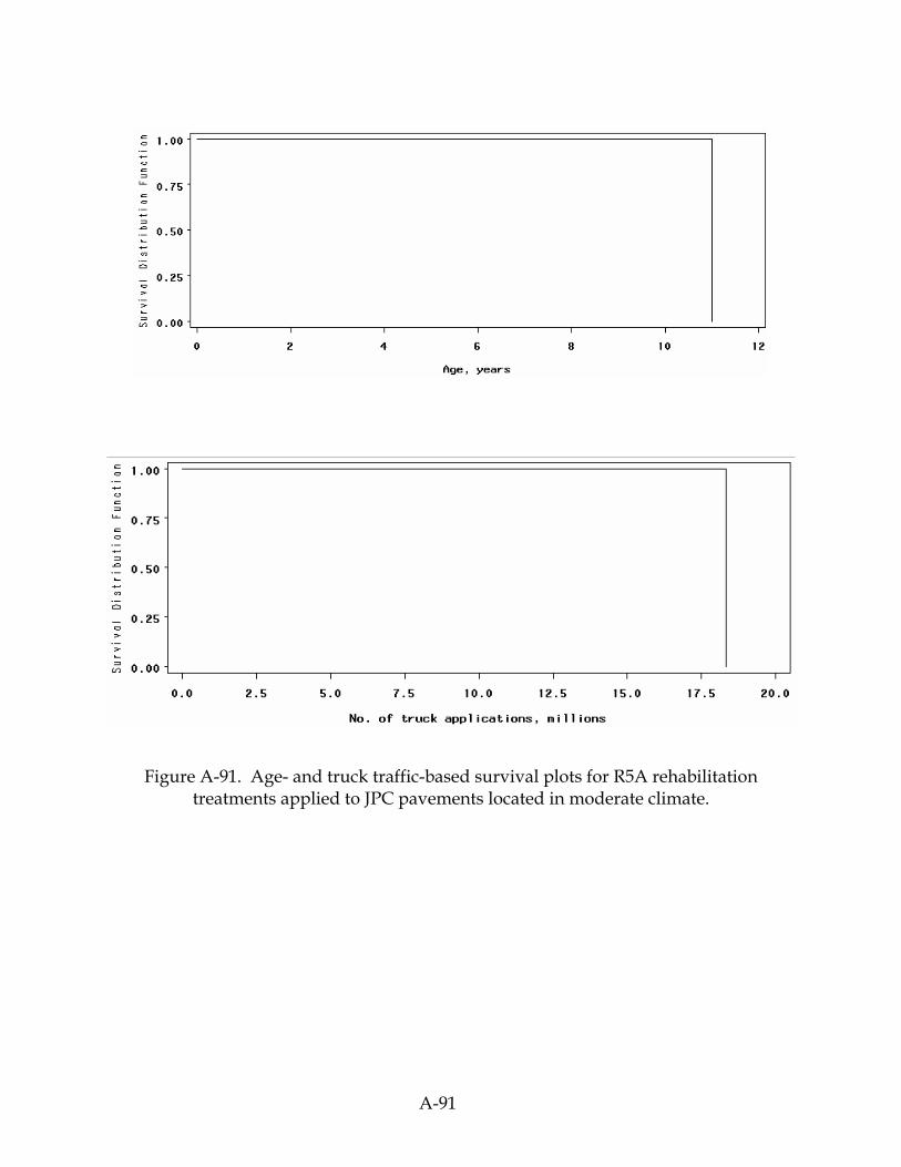
A-91
Figure A-91. Age- and truck traffic-based survival plots for R5A rehabilitation treatments applied to JPC pavements located in moderate climate.

A-92
Figure A-92. Age- and truck traffic-based survival plots for R5A rehabilitation treatments applied to JPC pavements located in cool-wet climate.

A-93
Figure A-93. Age- and truck traffic-based survival plots for R7 rehabilitation treatments
applied to JPC pavements located in hot-dry climate.

A-94
Figure A-94. Age- and truck traffic-based survival plots for R7 rehabilitation treatments
applied to JPC pavements located in moderate climate.

A-95
Figure A-95. Age- and truck traffic-based survival plots for R10B rehabilitation treatments applied to JPC pavements located in cool-wet climate.

A-96
Figure A-96. Age- and truck traffic-based survival plots for R12A rehabilitation treatments applied to JPC pavements located in cool-wet climate.

A-97
Figure A-97. Age- and truck traffic-based survival plots for R13B rehabilitation treatments applied to JPC pavements located in cool-wet climate.

A-98
Figure A-98. Age- and truck traffic-based survival plots for R7 rehabilitation treatments
applied to JPCD and CRC pavements located in hot-dry climate.