SpotFi: Decimeter Level Localization Using WiFi

Manikanta Kotaru, Kiran Joshi, Dinesh Bharadia, Sachin KattiStanford UniversityStanford, CA, USA

mkotaru, krjoshi, dineshb, skatti@stanford.edu

ABSTRACTThis paper presents the design and implementation of SpotFi,an accurate indoor localization system that can be deployedon commodity WiFi infrastructure. SpotFi only uses in-formation that is already exposed by WiFi chips and doesnot require any hardware or firmware changes, yet achievesthe same accuracy as state-of-the-art localization systems.SpotFi makes two key technical contributions. First, SpotFiincorporates super-resolution algorithms that can accuratelycompute the angle of arrival (AoA) of multipath componentseven when the access point (AP) has only three antennas.Second, it incorporates novel filtering and estimation tech-niques to identify AoA of direct path between the localiza-tion target and AP by assigning values for each path depend-ing on how likely the particular path is the direct path. Ourexperiments in a multipath rich indoor environment showthat SpotFi achieves a median accuracy of 40 cm and is ro-bust to indoor hindrances such as obstacles and multipath.

CCS Concepts•Information systems→ Location based services; Sensornetworks; Global positioning systems; •Networks→ Loca-tion based services;

KeywordsIndoor localization; Wireless; WiFi; OFDM; CSI

1. INTRODUCTIONIndoor localization systems using WiFi infrastructure sho-

uld ideally satisfy the following three requirements:• Deployable: They should be easily deployable on exist-

ing commodity WiFi infrastructure without requiring anyhardware or firmware changes at the access points (APs);they should only work with information like RSSI andCSI (Channel State Information) that is already exposedby commodity, deployed APs.

Permission to make digital or hard copies of all or part of this work for personalor classroom use is granted without fee provided that copies are not made ordistributed for profit or commercial advantage and that copies bear this noticeand the full citation on the first page. Copyrights for components of this workowned by others than the author(s) must be honored. Abstracting with credit ispermitted. To copy otherwise, or republish, to post on servers or to redistribute tolists, requires prior specific permission and/or a fee. Request permissions frompermissions@acm.org.

SIGCOMM ’15, August 17 - 21, 2015, London, United Kingdomc© 2015 Copyright held by the owner/author(s). Publication rights licensed to

ACM. ISBN 978-1-4503-3542-3/15/08. . . $15.00

DOI: http://dx.doi.org/10.1145/2785956.2787487

• Universal: They should be able to localize any target de-vice that has a commodity WiFi chip and nothing else.They should not require the target to have any other hard-ware, be it sensors such as accelerometers, gyroscopes,barometers, cameras, etc., or radios such as UWB, ultra-sound, Bluetooth LE, etc.• Accurate: They should be accurate, ideally as accurate as

the best known localization systems that use wireless sig-nals (even including those that do not satisfy the abovetwo requirements). To the best of our knowledge, themost accurate such localization systems are ArrayTrack [1]and Ubicarse [2] and these systems achieve an accuracyranging from 30–50 cm in office environments. Achiev-ing such accuracy would be the target.

If the above three requirements are satisfied, we can imagineindoor localization becoming a ubiquitous service like GPSthat can be installed on already deployed WiFi infrastructureand made available to any device with a WiFi chip.

However, to the best of our knowledge, no system that sat-isfies all three requirements exists. RSSI based systems aredeployable and universal, but are not accurate; their medianaccuracy ranges from 2–4 m [3, 4, 5]. Recent techniquesthat rely on angle of arrival (AoA) estimation such as Ar-rayTrack and LTEye [6] are accurate and universal but arenot deployable as they require hardware modifications. Forexample, ArrayTrack uses six to eight antennas whereas typ-ical APs have three, and LTEye requires motorized rotatingantennas which are not found on deployed APs. Other tech-niques that combine inputs from multiple sensors such asUbicarse [2] are accurate and deployable but not universal;they require that the target device has access to other sens-ing modes such as accelerometers, gyroscopes, etc., whichwould not be found on many devices (e.g., laptops, Nestthermostats). We refer the reader to Sec. 2 for a more de-tailed survey of related work and where different systems liewith respect to the above requirements.

The main contribution of this paper is a localization sys-tem that satisfies all the three requirements above. We presentSpotFi, an indoor localization system that provides a medianaccuracy of 40 cm using standard, commodity off-the-shelfWiFi radios, which is comparable to the best performing sys-tems such as ArrayTrack [1] and Ubicarse [2]. SpotFi re-quires no hardware or baseband firmware changes/additionsat the APs, nor does it need any calibration or fingerprintingof the environment. SpotFi’s localization targets also haveminimal requirements, they only require a commodity WiFichip.

269

SpotFi incorporates three techniques that enable it to achievethis combination of accuracy and deployment simplicity:• Super-resolution AoA Estimation: The first component

of SpotFi is a super-resolution AoA estimation algorithm,i.e., it accurately resolves all the AoAs of the indoor mul-tipath in spite of using just three antennas which is stan-dard in WiFi deployments today. The number of anten-nas limits the number of multipath components that onecan resolve. As prior work has noted [1, 2, 7, 8, 9], themore antennas there are, more multipath AoAs can beresolved more accurately. Our insight is that the multi-path not only creates measurable changes in CSI acrossantennas because of AoA but also affects CSI across sub-carriers because of time of flight (ToF, time taken by thesignal to reach the AP from the localization target).Using this fact, instead of just estimating AoA, SpotFicombines CSI values across subcarriers and antennas tojointly estimate AoA and ToF of each path. In the pro-cess, SpotFi creates a virtual sensor array with numberof elements greater than the number of multipath com-ponents, thus overcoming the constraint of limited an-tennas. Our unique insight here is that these joint AoAand ToF estimation algorithms can be implemented us-ing the CSI information that is already exposed by thecommodity WiFi cards. Using the AoA and ToF parame-ters estimated from CSI, we empirically demonstrate that,in commodity WiFi deployments, although the estimatedToF values are different from the absolute ToFs, the jointestimation procedure provides AoA accuracy that is com-parable to systems that require twice as many antennas [8]or non-standard configurations such as rotating antennasused in radar [6, 2].• Robust Direct Path Identification: SpotFi aims to find

the AoA of the direct path component in the multipathsignal from the target. However among the AoA esti-mates from the previous algorithm, the one correspond-ing to the direct path may be erroneous or may not evenexist due to several practical reasons such as noisy CSI,obstructed targets, weak signal strength from the targetand so on. The second key component of SpotFi is anovel algorithm that assigns values for each path depend-ing on the likelihood that the particular path is the directpath. This metric assignment algorithm enables SpotFi toeliminate AoA estimates that are very likely to be in errorand not belonging to the direct path component, therebyavoiding making large errors in localization.• Localization: The final step is a localization algorithm

that incorporates both the direct path AoA estimate fromthe above two steps as well as RSSI information avail-able from each of the APs to calculate the location of thetarget. Our key contribution here is a framework that ap-propriately weights the information from different APs totake into account how likely it is that the AoA measure-ment reported by each AP corresponds to the actual directpath between the target and that AP. This weighting of in-formation enables SpotFi to select information from APswith higher confidence metric and improve accuracy.

We implemented SpotFi using Intel 5300 commodity WiFi

cards. We strived to evaluate it under the same environmentsas the best performing systems ArrayTrack and Ubicarse [1,2]; we describe the testbed in Sec. 4. Our experiments showthat SpotFi achieves a median localization error of 40 cm,and the 80th percentile error is 1.8 m. To put these num-bers in context, the best performing prior system achievesa median error of 40 cm using 6 antennas per AP, whereasour APs have only three. We also show that SpotFi works ro-bustly in challenging scenarios; for example, it achieves verygood accuracy even when the target has strong direct pathsto only a couple of APs. Finally, we also show that SpotFiis lightweight and requires CSI measurements for only tenpackets from the target to localize accurately.

2. RELATED WORKIndoor localization using wireless infrastructure is a well-

studied problem. There is a large body of research which,for conciseness, we classify into four types: RSSI based,fingerprinting based, antenna array based, and time basedtechniques.RSSI based approaches: This class of systems measuresthe RSSI from the target at multiple APs, combines themvia triangulation along with a propagation model to locatethe target [3, 10, 4, 5, 11, 12, 13]. These systems are easyto deploy as RSSI values are easily available in current APs.However the best known systems in this space tend to achievea median accuracy of around 2–4 m [3, 4], and the 80th

percentile error is often as high as 5 m due to insufficientmodeling of RSSI which in practice depends not only on thelocation of the target but also on the changing environment.Fingerprinting based approaches: The idea of these ap-proaches is that one would collect fingerprints such as thevector of RSSIs from a specific location to all the APs inrange, and if in the future a target were at the same location,it would exhibit the same fingerprint, enabling us to local-ize [14, 15, 16, 17, 18, 19, 20, 21, 22]. The best known suchsystems provide around 0.6 m of median accuracy [14], andtail accuracy on the order of 1.3 m. However these systemsare difficult to deploy since they require an expensive and re-curring fingerprinting operation any time there are changesin the environment (e.g., when the furniture is moved).AoA based approaches: With the proliferation of WiFi APswith multiple antennas to support MIMO communications,antenna array based techniques which use multiple antennasat the AP have gained interest recently. The basic idea ofthese systems is to calculate the AoAs of the multipath sig-nals received at each AP, find the AoA of the direct path tothe target, and then apply triangulation to localize [1, 2, 6,23, 24, 8, 25]. The best known such systems have demon-strated significant improvements in accuracy with medianaccuracy on the order of 0.4 m [1, 2]. However these systemsare relatively difficult to deploy, since they require hardwarechanges by introducing as high as 8 antennas [1, 8], or newboxes itself with rotating antennas [6], or require special APsto access IQ samples [1, 24].

There are other recently proposed systems that use sensorssuch as gyroscopes, accelerometers, etc., along with AoA

270

AP2

AP1

AP3

Path 1 AoA, ToF

AP1

Path 2 AoA, ToF

Direct path AoA, ToF

AP1

AP2

AP1

AP3

Collect CSI from each AP and send it to a central server

server

Resolve multipath Identify direct path for each AP

Combine RSSI and AoA from all APs to localize target

Reflector

Target

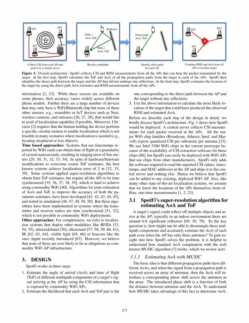
Figure 1: Overall architecture: SpotFi collects CSI and RSSI measurements from all the APs that can hear the packet transmitted by thetarget. In the first step, SpotFi calculates the ToF and AoA of all the propagation paths from the target to each of the APs. SpotFi thenidentifies the direct path between the target and the AP that did not undergo any reflections. In the final step, SpotFi estimates the location ofthe target by using the direct path AoA estimates and RSSI measurements from all the APs.

information [2, 23]. While these sensors are available onsome phones, their accuracy varies widely across differentphone models. Further there are a large number of devicesthat may only have a WiFi/Bluetooth chip but none of theseother sensors, e.g., wearables or IoT devices such as Nest,wireless cameras, and suitcases [26, 27, 28], that would liketo avail of localization capability if possible. Moreover, Ubi-carse [2] requires that the human holding the device performa specific circular motion to enable localization which is notfeasible in many scenarios where localization is needed (e.g.,locating misplaced or lost objects).Time based approaches: Systems that use timestamps re-ported by WiFi cards can obtain time of flight at a granularityof several nanoseconds, resulting in ranging error of few me-ters [29, 30, 31, 32, 33, 34]. In spite of hardware/firmwaremodifications to overcome coarse ToF estimates, the bestknown systems achieve localization error of 2 m [32, 33,30]. Some systems applied super-resolution algorithms toobtain finer ToF estimates, but require all the APs to be timesynchronized [35, 36, 37, 38, 39], which is hard to achieveusing commodity WiFi [40]. Algorithms for joint estimationof AoA and ToF, to improve the accuracy of both the pa-rameter estimates, have been developed [41, 42, 43, 44, 45],and tested in simulation [46, 47, 48, 49, 50]. But these algo-rithms have been implemented in systems where the trans-mitter and receiver radios are time synchronized [51, 52],which is not possible in commodity WiFi deployments.Other approaches: For completeness, we refer to localiza-tion systems that deploy other modalities like RFIDs [53,54, 55], ultrawideband [56], ultrasound [57, 58, 59, 60, 61],IR [62, 63, 64], visible light [65, 66] or beacons like theones Apple recently introduced [67]. However, we believethat none of these are ever likely to be as ubiquitous as com-modity WiFi AP infrastructure.

3. DESIGNSpotFi works in three steps:

1. Estimate the angle of arrival (AoA) and time of flight(ToF) of different multipath components of a target’s sig-nal arriving at the AP by using the CSI information thatis exposed by commodity WiFi APs.

2. Estimate the likelihood that each AoA and ToF pair is the

one corresponding to the direct path between the AP andthe target without any reflections.

3. Use the above information to calculate the most likely lo-cation of the target that could have produced the observedRSSI and estimated AoA.

Before we describe each step of the design in detail, webriefly discuss SpotFi’s architecture. Fig. 1 shows how SpotFiwould be deployed. A central server collects CSI measure-ments for each packet received at the APs. All the ma-jor WiFi chip families (Broadcom, Atheros, Intel, and Mar-vell) expose quantized CSI per subcarrier per antenna [23].We use Intel 5300 WiFi chips in the current prototype be-cause of the availability of CSI extraction software for thesechips [68], but SpotFi can easily be deployed with WiFi APsthat use chips from other manufacturers. SpotFi only addsthe software required to read the reported CSI values, times-tamps, and MAC addresses at the AP and ships it to the cen-tral server and nothing else. Hence we believe that SpotFican be added to any existing, deployed WiFi AP. Also, likemany other state-of-the-art localization systems, we assumethat we know the locations of the APs themselves from of-fline, one-time measurements [1, 2, 23].

3.1 SpotFi’s super-resolution algorithm forestimating AoA and ToF

A target’s signal could reflect off multiple objects and ar-rive at the AP; typically in an indoor environment there arearound 6-8 significant reflectors [69, 30, 70]. So the keyquestion is, how might one be able to disentangle these mul-tipath components and accurately estimate the AoA of eachpath even when the AP has only three antennas? To gain in-sight into how SpotFi solves the problem, it is helpful tounderstand how standard AoA computation with the wellknown MUSIC algorithm [7] works, which we review next.

3.1.1 Estimating AoA with MUSICThe basic idea is that different propagation paths have dif-

ferent AoAs, and when the signal from a propagation path isreceived across an array of antennas, then the AoA will in-troduce a corresponding phase shift across the antennas inthe array. The introduced phase shift is a function of boththe distance between antennas and the AoA. To understandhow MUSIC takes advantage of this fact to determine AoA,

271

. . .

1 2 Md

Antenna Array

Incident Signal

d.sin𝜽

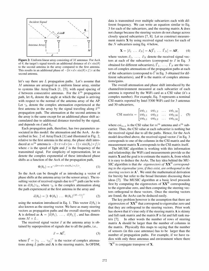
Figure 2: Uniform linear array consisting ofM antennas: For AoAof θ, the target’s signal travels an additional distance of d× sin(θ)to the second antenna in the array compared to the first antenna.This results in an additional phase of −2π×d× sin(θ)×f/c at thesecond antenna.

let’s say there are L propagation paths. Let’s assume thatM antennas are arranged in a uniform linear array, similarto systems like ArrayTrack [1, 23], with equal spacing ofd between consecutive antennas. For the kth propagationpath, let θk denote the angle at which the signal is arrivingwith respect to the normal of the antenna array of the AP.Let γk denote the complex attenuation experienced at thefirst antenna in the array by the signal traveling along kth

propagation path. The attenuation at the second antenna inthe array is the same except for an additional phase shift ac-cumulated due to additional distance traveled by the signal,and depends on d and θk.

Each propagation path, therefore, has two parameters as-sociated in this model: the attenuation and the AoA. As de-scribed in Sec. 2 of ArrayTrack [1] and illustrated in Fig. 2,relative to the first antenna in the array, the phase shift intro-duced at mth antenna is −2×π×d×(m− 1)× sin(θk)×f/cwhere c is the speed of light and f is the frequency of thetransmitted signal. For simplicity of representation, let usdenote the complex exponential of these introduced phaseshifts as a function of the AoA of the propagation path,

Φ(θk) = e−j2π×d× sin(θk)×f/c. (1)

So the AoA can be thought of as introducing a vector ofphase shifts at the antenna array (or the sensor array). The re-sulting vector of received signals due to kth path can be writ-ten as ~a(θk)γk, where γk is the complex attenuation alongthe path experienced at the first antenna in the array and

~a(θk) = [1 Φ(θk) . . . Φ(θk)(M−1)]> (2)

using the notation introduced in Eq. 1. This vector ~a(θk) isalso known as the steering vector. We have as many steeringvectors as propagation paths and the overall steering matrixA is defined as A = [~a(θ1), . . . , ~a(θL)] , and has dimen-sions M × L .

The received signal vector ~x at the antenna array is ob-tained by superposition of signals due to all the paths, i.e.,

~x = A~Γ, (3)

where ~Γ = [γ1 . . . γL]> is the vector of complex attenua-tions along L paths and A is the steering matrix. In OFDM,

data is transmitted over multiple subcarriers each with dif-ferent frequency. We can write an equation similar to Eq.3 for each of the subcarriers, and the steering matrix A doesnot change because the steering vectors do not change acrossclosely spaced subcarriers [7, 8]. Let us construct measure-ment matrix X by using received signal vectors for each ofthe N subcarriers using Eq. 4 below,

X = [~x1 . . . ~xN ] = A[~Γ1 . . . ~ΓN ] = AF, (4)

where vectors ~x1, . . . , ~xN denote the received signal vec-tors at each of the subcarriers (correspond to ~x in Eq. 3obtained for different subcarriers), ~Γ1, . . . , ~ΓN are the vec-tors of complex attenuations of the propagation paths at eachof the subcarriers (correspond to ~Γ in Eq. 3 obtained for dif-ferent subcarriers), and F is the matrix of complex attenua-tions/gains.

The overall attenuation and phase shift introduced by thechannel/environment measured at each subcarrier of eachantenna is reported by the WiFi card as a CSI value (it’s acomplex number). For example, Eq. 5 represents a nominalCSI matrix reported by Intel 5300 WiFi card for 3 antennasand 30 subcarriers,

CSI matrix =

csi1,1 csi1,2 . . . csi1,30csi2,1 csi2,2 . . . csi2,30csi3,1 csi3,2 . . . csi3,30

, (5)

where csim,n is the CSI value for mth antenna and nth sub-carrier. Thus, the CSI value at each subcarrier is nothing butthe received signal due to all the paths. Hence, for the AoAmodel described above, the received signal vector ~x in Eq. 3corresponds to one of the columns in the CSI matrix and themeasurement matrix X corresponds to the CSI matrix itself.

The MUSIC algorithm is working with this informationand relationship; the WiFi card measurements provide us thematrix X and the goal is to estimate the matrix A, from whichit is easy to deduce the AoAs. The key idea behind the MU-SIC algorithm is that the eigenvectors of XXH correspond-ing to the eigenvalue zero, if they exist, are orthogonal to thesteering vectors in A1. We omit the mathematical derivationfor brevity but refer to the broad literature discussing theseideas [7]. The MUSIC algorithm at a basic level proceedsfirst by computing the eigenvectors of XXH correspondingto the eigenvalue zero, and then computing the steering vec-tors orthogonal to these vectors. Once the steering vectorsare found, the AoAs can be deduced easily.

The key problem however is the assumption that there areeigenvectors of XXH that correspond to eigenvalue zero andthat they are orthogonal to the steering vectors. Prior workhas shown that it’s true only if the steering matrix A is skinnyand full rank matrix and the matrix F is fat and full rank ma-trix [7]. In other words the number of rows of steeringmatrix A should be larger than the number of columns inthe matrix. Physically this maps to saying that the numberof sensors (in this case antennas) has to be larger than thenumber of propagation paths. For example, if we have ra-dios with only three antennas and environment where there1XH is conjugate transpose of X.

272

are more than three significant propagation paths (which isquite likely), the above algorithm doesn’t work well. This isthe reason past works have either used more antennas (eightin ArrayTrack [1]) or used rotating antennas to simulate alarger antenna array (e.g., LTEye [6]). Also, the number ofcolumns of matrix F of complex gains should be greater thanthe number of its rows, i.e., number of measurements at thesensor array should be greater than the number of paths.

3.1.2 Super-Resolution AoA EstimationHow might one increase the resolution of AoA estima-

tion? From the above discussion it’s clear that the key factoris the number of sensors from which we can measure proper-ties of the propagation paths and the number of independentmeasurements we can obtain at the sensor array. SpotFi’sinsight is that the number of sensors is not limited by thenumber of antennas, but in fact by leveraging the fact thatWiFi has many OFDM subcarriers on each of which we geta CSI measurement, the number of sensors can be expandedto be equal to the product of the number of subcarriers andthe number of antennas. For example, for Intel 5300 WiFicards, number of sensors would be equal to 30×3 = 90 sen-sors rather than the 3 antennas with the modeling describedin Sec. 3.1.1.

However, if each sensor in this extended sensor array ismodeled to measure just AoAs of the paths, then the numberof distinct values in our parametric model of sensor mea-surements is still limited by the number of antennas. This isbecause AoA of a propagation path does not manifest itselfin any measurable way across subcarriers, i.e., AoA does notintroduce any phase shift across subcarriers of an antenna.This is easy to see given that the relative phase shift intro-duced by AoA of the kth path across two subcarriers of themth antenna is 2π(m−1)d(fi−fj) sin(θk)/c, where fi andfj denote the frequencies of the two subcarriers. So, withhalf-wavelength antenna spacing, for two subcarriers of thesecond antenna separated by 40 MHz, any AoA introducesa phase shift of at most 0.002 radians which is negligible.Hence, phase shift due to AoA is same across all the sub-carriers of an antenna since the speed of light factor in thedenominator is much larger than this small frequency differ-ence. So, although there are 90 subcarriers (from all threeantennas combined) in Intel 5300 CSI measurements, only2 distinct phase shifts are introduced due to AoA, since wecompute phase shifts relative to the first antenna and thereare three antennas.Obtaining sensor array larger than the number of paths:SpotFi’s key insight is counterintuitive. Instead of just es-timating AoA per propagation path, SpotFi proposes to alsocalculate the time of flight (ToF) for each path. By definitioneach path will likely have a different ToF too. The reason toadd ToF as a parameter for each path is that it introducesmeasurable phase shifts across subcarriers. For example thephase shift across two subcarriers even across the same an-tenna for the kth path with ToF τk is given by 2π(fi−fj)τkwhich is significant (the reason numerically is the lack of thespeed of light factor in the denominator). Here, fi and fjdenote the frequencies of the two subcarriers as before. For

example, for two subcarriers spaced apart by 40 MHz andfor ToF of 10 ns, there is significant difference of 2.5 radiansin the phase shift introduced at the two subcarriers. Specifi-cally, for equispaced OFDM subcarriers, kth path with ToFτk introduces a phase shift of−2×π×(n−1)×fδ×τk at thenth subcarrier relative to the first subcarrier of an antenna,where fδ is the frequency spacing between two consecutivesubcarriers. For simplicity of representation, let us denotethe complex exponential of the phase shift introduced be-tween two adjacent subcarriers as a function of the ToF,

Ω(τk) = e−j2×π×fδ×τk . (6)

SpotFi exploits this insight to expand the number of sensors,and specifically design a steering matrix A that is skinny andenables the resolution of all the paths.

Specifically, consider the sensor array comprising of allthe subcarriers at all the antennas. The measurement matrixX is constructed by stacking CSI from all the subcarriers atall the antennas, and hence is a single column matrix. Eachpropagation path introduces a distinct phase shift at each ofthe sensors depending both on its ToF and AoA. So, for apath with AoA θ and ToF τ , the steering vector, for the M ×N sensors (M antennas times N subcarriers), is formed byphase shifts introduced at each of the sensors due to bothAoA and ToF, and is given by:

~a(θ, τ) =[

antenna 1︷ ︸︸ ︷1, . . . ,ΩN−1

τ ,Φθ, . . . ,ΩN−1

τ Φθ︸ ︷︷ ︸antenna 2

, . . . ,

antenna M︷ ︸︸ ︷ΦM−1

θ , . . . ,ΩN−1

τ ΦM−1

θ ]>,

(7)where Ω(τ) is written as Ωτ and Φ(θ) as Φθ for brevity.

CSI at each sensor is a linear combination of the phaseshifts introduced due to all the paths weighted by their atten-uations. So, the newly constructed measurement matrix Xis nothing but a linear combination of the steering vectors inEq. 7 evaluated for all the paths. Note that phase of complexattenuation in the model described in Eq. 3 has the phaseshift due to ToF absorbed into it and is different for differentsubcarriers, whereas here the phase of attenuation just de-pends on the objects that the signal interacted with along thepath and is same for all the subcarriers of all the antennas.The steering matrix corresponding to this extended sensorarray still has number of columns equal to the number ofpaths. We have thus increased the number of sensors with-out increasing the number of paths, i.e., we have achieved askinny steering matrix A .

The other fact to note from the previous section’s descrip-tion of MUSIC is that the number of measurements at thesensor array, that can be written as linear combination of thesame steering vectors, should be greater than the number ofpaths. However, the measurement matrix obtained by stack-ing CSI from all the subcarriers at all the antennas is a singlecolumn unit rank matrix. We now describe how we obtaina measurement matrix with number of columns greater thannumber of paths.CSI smoothing: SpotFi’s mathematical trick to obtain a sen-sor array with multiple independent measurements is bestdemonstrated through an example. Let’s say there are L = 2

273

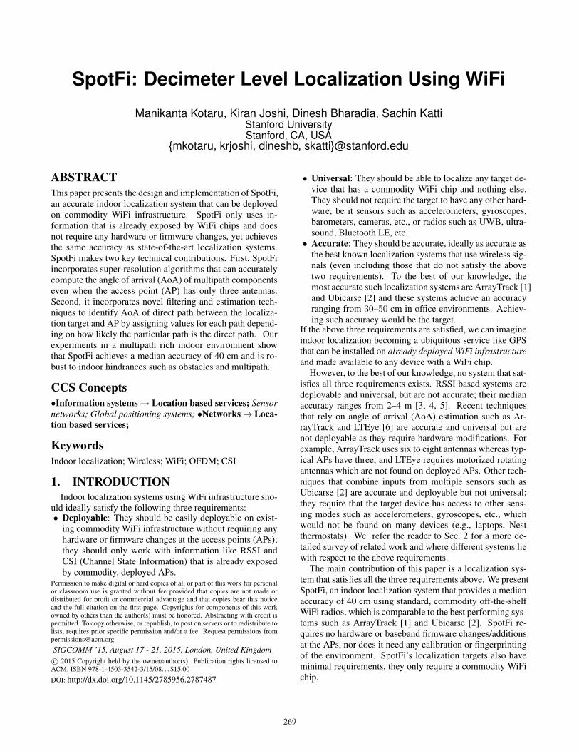
(a) Entries of the steering vector

(b) CSI values at the two sensor subarrays

5 subcarriers

CSI values at the two subarrays

Same steering matrix

Independent vectors of gains

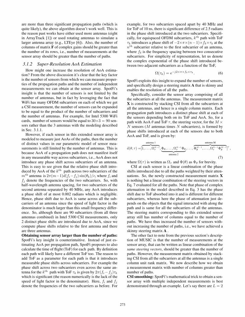
Figure 3: (a) The elements of the steering vector in Eq. 7 for twosubsets of sensors. The elements in the dashed red box (second sen-sor subarray) are obtained by scaling the corresponding elementsin solid blue box (first subarray) by Ω2(τk)Φ(θk). Ωτk representsΩ(τk) and Φθk represents Φ(θk). (b) csim,n represents the CSIobtained at nth subcarrier and mth antenna. So, the two columnson the left hand side of the equation correspond to the CSI valuesobtained at the two sensor subarrays displayed in (a). CSI mea-surements obtained for the second sensor subarray are obtained bycombining the same steering vectors as the first sensor subarraybut with different independent vector of weights. The CSI mea-surements and the vector of gains corresponding to the first sensorsubarray are colored blue and similarly the corresponding valuesfor second sensor subarray are colored red.

paths. Consider the CSI at the subcarriers corresponding totwo sensor subarrays displayed in the two columns of thematrix on the left hand side (LHS) of equation in Fig. 3(b).First sensor subarray, corresponding to the first column ofFig. 3(b), is comprised of first three subcarriers at antennas1 and 2. The second sensor subarray, corresponding to thesecond column of Fig. 3(b), is comprised of subcarriers 3 to5 at antennas 2 and 3. We will show in the following para-graphs that the measurements at these two sensor subarrayscan be written as linear combination of the same vectors, butwith different gains, as illustrated in Fig. 3(b). So, if we canidentify L such sensor subarrays whose CSI values can bewritten as linear combination of same vectors, then the MU-SIC algorithm can be applied on the measurement matrixobtained from the CSI measurements at these subarrays.

To gain intuition into why CSI at the two sensor subar-rays shown in Fig. 3(b) can be written as linear combinationof same vectors, let’s look at the entries of steering vectorin Eq. 7 evaluated for kth propagation path as illustrated inFig. 3(a). The phase shifts in the solid blue box correspondto the steering vector entries of the first sensor subarray andthe phase shifts in the dashed red box correspond to those

in the second sensor subarray. We observe that the phaseshift between the corresponding elements of the two sensorsubarrays are related through a common scaling factor. Forexample, phase shift of the top left sensor of second sen-sor subarray, i.e., subcarrier 3 at antenna 2, is obtained bymultiplying phase shift at the top left sensor of the first sen-sor subarray, i.e., subcarrier 1 at antenna 1, by Ω2(τk)Φ(θk).This scaling factor is infact the phase shift term we wouldsee for this propagation path for a shift of 2 subcarriers and1 antenna, and is expected since both the sensor subarraysare structurally same except for a shift of 2 subcarriers and1 antenna. The common scaling factor, Ω2(τk)Φ(θk), de-pends on the relative shift in antennas and subcarriers of thetwo sensor subarrays as well as the propagation path param-eters, and hence is different for different paths. How can oneexploit the above insight?

Let α1 and α2 be the complex gains along the two paths.We obtain CSI values at the sensors belonging to first sub-array by weighing the corresponding steering vector entriesfor the two paths by their complex gains α1 and α2 (see Fig.3(b)), and similarly for the second sensor subarray. How-ever, by absorbing common scaling factor Ω2(τk)Φ(θk) intothe complex gains at the second subarray, we can write theCSI values at the second sensor subarray by weighing thesteering vector entries corresponding to first subarray forthe two paths with the modified gains Ω2(τ1)Φ(θ1)α1 andΩ2(τ2)Φ(θ2)α2. The same is illustrated in Fig. 3(b). Wehave thus shown that CSI at these two sensor subarrays canbe written as linear combination of the same vectors. More-over, the vector of complex gains of the second subarray islinearly independent of the vector of the complex gains offirst subarray, because attenuations corresponding to differ-ent paths are multiplied by different factors to obtain modi-fied gains at the second subarray.

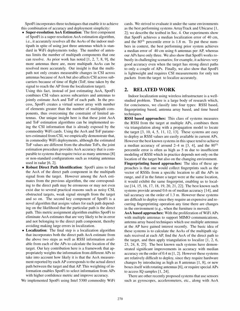
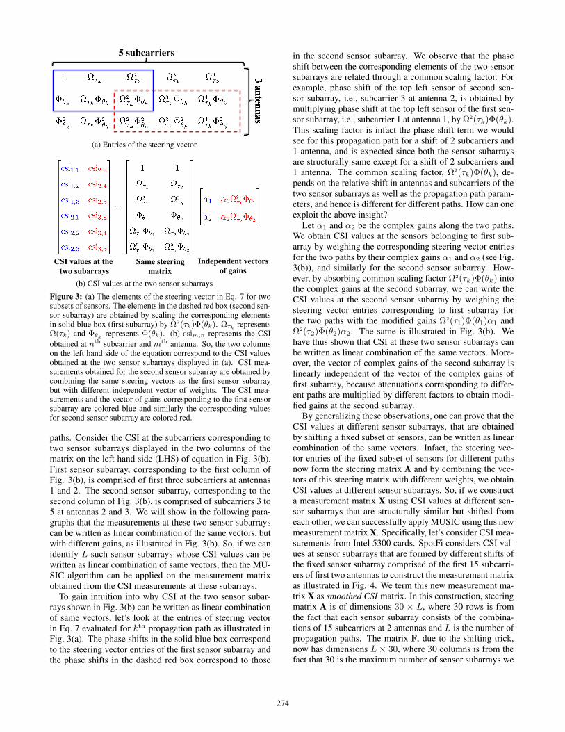
By generalizing these observations, one can prove that theCSI values at different sensor subarrays, that are obtainedby shifting a fixed subset of sensors, can be written as linearcombination of the same vectors. Infact, the steering vec-tor entries of the fixed subset of sensors for different pathsnow form the steering matrix A and by combining the vec-tors of this steering matrix with different weights, we obtainCSI values at different sensor subarrays. So, if we constructa measurement matrix X using CSI values at different sen-sor subarrays that are structurally similar but shifted fromeach other, we can successfully apply MUSIC using this newmeasurement matrix X. Specifically, let’s consider CSI mea-surements from Intel 5300 cards. SpotFi considers CSI val-ues at sensor subarrays that are formed by different shifts ofthe fixed sensor subarray comprised of the first 15 subcarri-ers of first two antennas to construct the measurement matrixas illustrated in Fig. 4. We term this new measurement ma-trix X as smoothed CSI matrix. In this construction, steeringmatrix A is of dimensions 30 × L, where 30 rows is fromthe fact that each sensor subarray consists of the combina-tions of 15 subcarriers at 2 antennas and L is the number ofpropagation paths. The matrix F, due to the shifting trick,now has dimensions L × 30, where 30 columns is from thefact that 30 is the maximum number of sensor subarrays we

274

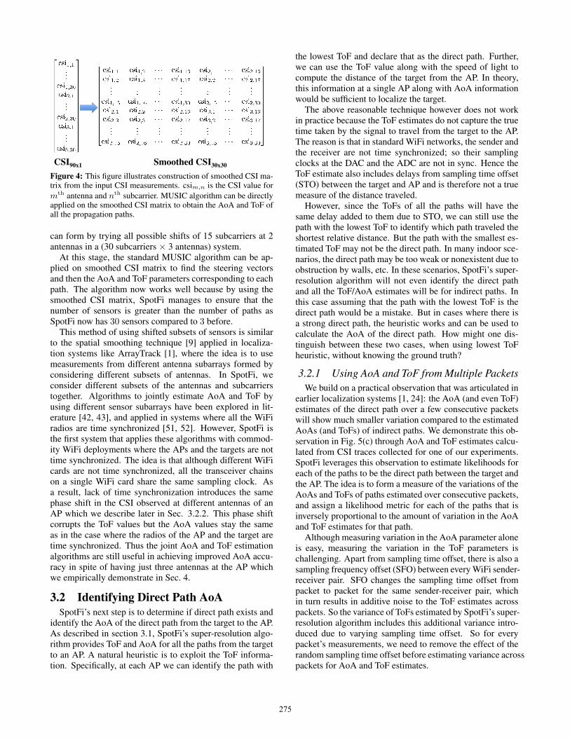
CSI90x1 Smoothed CSI30x30 Figure 4: This figure illustrates construction of smoothed CSI ma-trix from the input CSI measurements. csim,n is the CSI value formth antenna and nth subcarrier. MUSIC algorithm can be directlyapplied on the smoothed CSI matrix to obtain the AoA and ToF ofall the propagation paths.

can form by trying all possible shifts of 15 subcarriers at 2antennas in a (30 subcarriers × 3 antennas) system.

At this stage, the standard MUSIC algorithm can be ap-plied on smoothed CSI matrix to find the steering vectorsand then the AoA and ToF parameters corresponding to eachpath. The algorithm now works well because by using thesmoothed CSI matrix, SpotFi manages to ensure that thenumber of sensors is greater than the number of paths asSpotFi now has 30 sensors compared to 3 before.

This method of using shifted subsets of sensors is similarto the spatial smoothing technique [9] applied in localiza-tion systems like ArrayTrack [1], where the idea is to usemeasurements from different antenna subarrays formed byconsidering different subsets of antennas. In SpotFi, weconsider different subsets of the antennas and subcarrierstogether. Algorithms to jointly estimate AoA and ToF byusing different sensor subarrays have been explored in lit-erature [42, 43], and applied in systems where all the WiFiradios are time synchronized [51, 52]. However, SpotFi isthe first system that applies these algorithms with commod-ity WiFi deployments where the APs and the targets are nottime synchronized. The idea is that although different WiFicards are not time synchronized, all the transceiver chainson a single WiFi card share the same sampling clock. Asa result, lack of time synchronization introduces the samephase shift in the CSI observed at different antennas of anAP which we describe later in Sec. 3.2.2. This phase shiftcorrupts the ToF values but the AoA values stay the sameas in the case where the radios of the AP and the target aretime synchronized. Thus the joint AoA and ToF estimationalgorithms are still useful in achieving improved AoA accu-racy in spite of having just three antennas at the AP whichwe empirically demonstrate in Sec. 4.

3.2 Identifying Direct Path AoASpotFi’s next step is to determine if direct path exists and

identify the AoA of the direct path from the target to the AP.As described in section 3.1, SpotFi’s super-resolution algo-rithm provides ToF and AoA for all the paths from the targetto an AP. A natural heuristic is to exploit the ToF informa-tion. Specifically, at each AP we can identify the path with

the lowest ToF and declare that as the direct path. Further,we can use the ToF value along with the speed of light tocompute the distance of the target from the AP. In theory,this information at a single AP along with AoA informationwould be sufficient to localize the target.

The above reasonable technique however does not workin practice because the ToF estimates do not capture the truetime taken by the signal to travel from the target to the AP.The reason is that in standard WiFi networks, the sender andthe receiver are not time synchronized; so their samplingclocks at the DAC and the ADC are not in sync. Hence theToF estimate also includes delays from sampling time offset(STO) between the target and AP and is therefore not a truemeasure of the distance traveled.

However, since the ToFs of all the paths will have thesame delay added to them due to STO, we can still use thepath with the lowest ToF to identify which path traveled theshortest relative distance. But the path with the smallest es-timated ToF may not be the direct path. In many indoor sce-narios, the direct path may be too weak or nonexistent due toobstruction by walls, etc. In these scenarios, SpotFi’s super-resolution algorithm will not even identify the direct pathand all the ToF/AoA estimates will be for indirect paths. Inthis case assuming that the path with the lowest ToF is thedirect path would be a mistake. But in cases where there isa strong direct path, the heuristic works and can be used tocalculate the AoA of the direct path. How might one dis-tinguish between these two cases, when using lowest ToFheuristic, without knowing the ground truth?

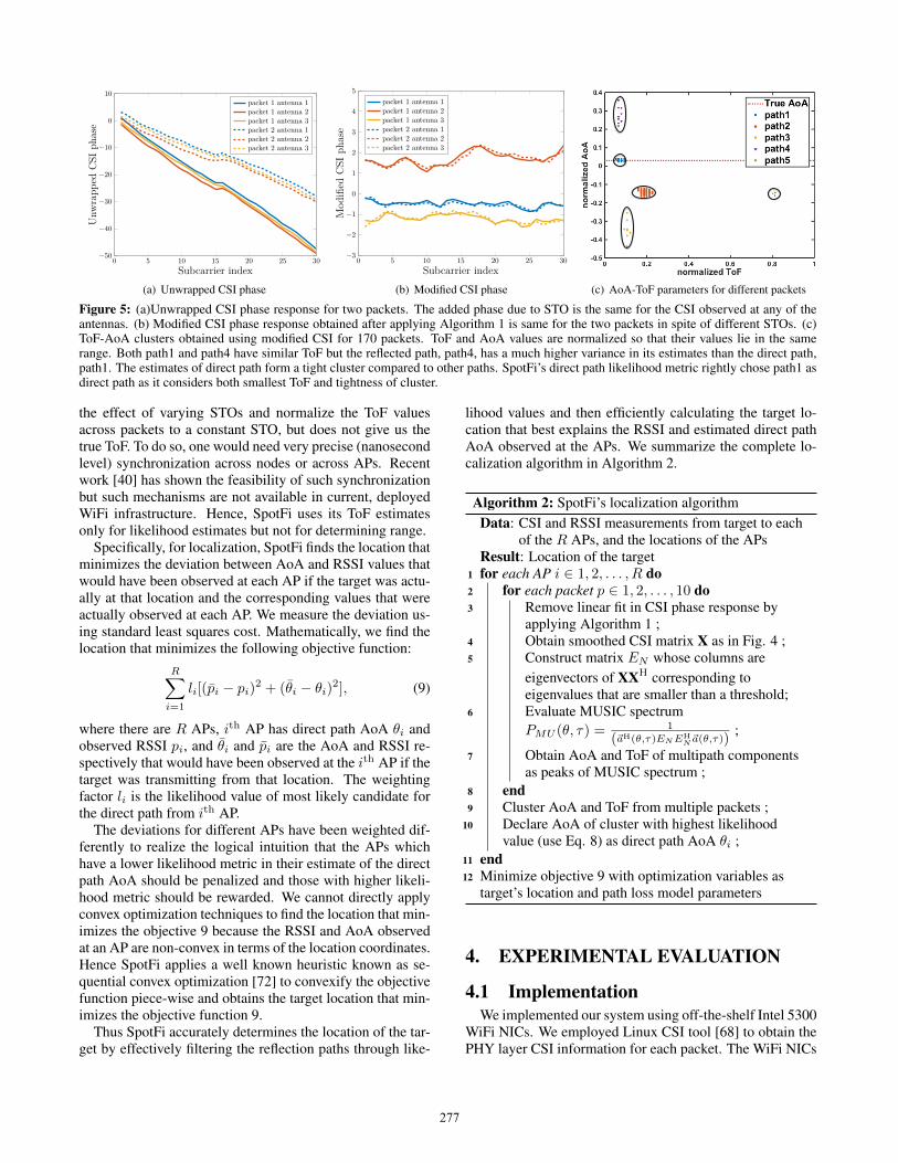
3.2.1 Using AoA and ToF from Multiple PacketsWe build on a practical observation that was articulated in

earlier localization systems [1, 24]: the AoA (and even ToF)estimates of the direct path over a few consecutive packetswill show much smaller variation compared to the estimatedAoAs (and ToFs) of indirect paths. We demonstrate this ob-servation in Fig. 5(c) through AoA and ToF estimates calcu-lated from CSI traces collected for one of our experiments.SpotFi leverages this observation to estimate likelihoods foreach of the paths to be the direct path between the target andthe AP. The idea is to form a measure of the variations of theAoAs and ToFs of paths estimated over consecutive packets,and assign a likelihood metric for each of the paths that isinversely proportional to the amount of variation in the AoAand ToF estimates for that path.

Although measuring variation in the AoA parameter aloneis easy, measuring the variation in the ToF parameters ischallenging. Apart from sampling time offset, there is also asampling frequency offset (SFO) between every WiFi sender-receiver pair. SFO changes the sampling time offset frompacket to packet for the same sender-receiver pair, whichin turn results in additive noise to the ToF estimates acrosspackets. So the variance of ToFs estimated by SpotFi’s super-resolution algorithm includes this additional variance intro-duced due to varying sampling time offset. So for everypacket’s measurements, we need to remove the effect of therandom sampling time offset before estimating variance acrosspackets for AoA and ToF estimates.

275

3.2.2 Sanitizing ToF EstimatesSTO adds a constant offset to the ToF estimates of all the

paths. This common additional delay manifests itself as alinear in frequency term in the phase response of the chan-nel. Hence, STO of τs results in adding −2πfδ(n − 1)τsto the phase of CSI value of the nth subcarrier. The addi-tional phase induced by STO is the same across antennas fora particular subcarrier, as all the receiver chains of the sameWiFi card are time synchronized. We will now show that re-moving the linear fit that is common to the unwrapped phaseresponse of all the antennas before estimating multipath pa-rameters eliminates the varaiance due to changing STO.

Let us consider two consecutive packets transmitted bythe target. Letψi(m,n) represent unwrapped phase responseof the channel for the ith packet at nth subcarrier of mth an-tenna, and τs,i is the STO for ith packet. By applying ToFsanitization algorithm described in Algorithm 1, say we re-moved the linear fit of CSI phase response for first packet toobtain modified phase response ψ1(m,n).

Algorithm 1: SpotFi’s ToF sanitization algorithm

Data: Unwrapped CSI phase ψi for ith packet1 Obtain the best linear fit of the unwrapped CSI phase as

τs,i = arg minρ

M,N∑m,n=1

(ψi(m,n) + 2πfδ(n− 1)ρ + β)2

;

2 From the unwrapped CSI phase, subtract the phase thatwould have been added due to STO τs,i to obtainmodified CSI phase ψi(m,n) asψi(m,n) = ψi(m,n) + 2πfδ(n− 1)τs,i

Phase response of second packet ψ2 can be written asψ2(m,n) = ψ1(m,n) − 2πfδ(n− 1)(τs,2 − τs,1). Usingthis relationship, one can prove that the modified CSI phaseof the second packet is given by ψ2(m,n) = ψ1(m,n) +2πfδ(n − 1)τs,1, which is same as the modified CSI phaseof first packet. The actual and modified CSI phase responsesfor two packets obtained from CSI traces collected from ourexperiments are presented in Fig. 5(a) and Fig. 5(b) re-spectively. The modified CSI phase response, obtained byapplying Algorithm 1 for each packet, does not change evenif the STO changes, and hence is free from the variations ofSTO. So, the ToF parameters estimated across packets usingmodified CSI are free from variance of changing STO. Wenote that the Algorithm 1 is similar to the data sanitizationprocess in PinLoc [15] and is an extension of the processto multiple antennas. We also note that although we havediscussed changes in ToF due to SFO alone, the variancein ToF due to random packet detection delay [40] can alsoeliminated by following Algorithm 1.

3.2.3 Estimating Direct Path LikelihoodsNow we have a collection of AoA and ToF estimates whose

variance across packets can be estimated. To assign like-lihood estimates for each of the estimated paths to be the

direct path between the target and AP, we plot AoA and ToFestimates from multiple measurements in a two- dimensional(one each for AoA and ToF) space and apply a clustering al-gorithm. The intuition is that AoA and ToF estimates fromthe same path but different packets will be clustered together,but the diameter of each cluster (i.e., the tightness of eachcluster) will be a function of the variations in AoA and ToFvalues for the corresponding path across packets.

Specifically, we use well-known Gaussian Mean cluster-ing algorithm with five clusters to identify the clusters of theestimated parameters. The number of clusters is chosen asfive because typically we see at best five significant paths inan indoor environment [1, 8, 24]. The mean of a cluster isused as an estimate for the actual ToF and AoA of the partic-ular propagation path. The variance in the ToF of a path isestimated by calculating the population variance of the ToFestimates belonging to the cluster of the particular path, andsimilarly for AoA. Then the likelihood for kth path to be thedirect path is calculated as

likelihoodk = exp(wCCk−wθσθk −wτ στk −wsτk), (8)

where likelihoodk is the likelihood that the kth path is thedirect path, Ck is the number of points in the cluster corre-sponding to that path, σθk and στk are the population vari-ances of the estimated AoA and ToF respectively for pointsbelonging to that cluster, and τk is the mean of ToF for pointsin that cluster. The weighting factorswC ,wθ,wτ , andws areconstants to account for different scales of the correspond-ing terms (for example, ToF values are on the order of ns andnumber of points in the cluster is on the order of 10).

The likelihood estimate incorporates a few other termsapart from the tightness of the cluster. First is the term corre-sponding to the number of points in the cluster. The insighthere is that if a cluster corresponds to a physical propaga-tion path, then it is likely to have more measurements thana cluster which is spurious and doesn’t correspond to an un-derlying physical path. The intuition for the term related tothe mean ToF is that the direct path will have the smallestToF, so a higher ToF term should signify a lower likelihood.

SpotFi declares the path with the highest likelihood metricas the direct path, and stores the AoA and the likelihoodvalue of the corresponding path.

3.3 Localizing the TargetNext, SpotFi attempts to localize the target by combin-

ing the direct path AoA estimates and their likelihood valuescorresponding to different APs. Further, the server also hasthe access to the RSSI measurements for the packets fromthe target to each AP that “heard" the target. The server as-sumes a standard widely used path loss model to relate RSSIto distance as described in prior work [3, 71]. The serverthen fuses all this information to localize the target.

To localize, SpotFi finds the location that best explains theAoA and RSSI measurements at different APs. We do notuse the ToF information to form distance estimates becauseit still does not capture the true ToF of the signal from the tar-get to the AP. The procedure described in Sec. 3.2.2 to scrubany distortion in the ToF estimates only helps in removing

276

0 5 10 15 20 25 30−50

−40

−30

−20

−10

0

10

Subcarrier index

Unw

rapp

edC

SIph

ase

packet 1 antenna 1packet 1 antenna 2packet 1 antenna 3packet 2 antenna 1packet 2 antenna 2packet 2 antenna 3

(a) Unwrapped CSI phase

0 5 10 15 20 25 30−3

−2

−1

0

1

2

3

4

5

Subcarrier index

Mod

ified

CSI

phase

packet 1 antenna 1packet 1 antenna 2packet 1 antenna 3packet 2 antenna 1packet 2 antenna 2packet 2 antenna 3

(b) Modified CSI phase (c) AoA-ToF parameters for different packets

Figure 5: (a)Unwrapped CSI phase response for two packets. The added phase due to STO is the same for the CSI observed at any of theantennas. (b) Modified CSI phase response obtained after applying Algorithm 1 is same for the two packets in spite of different STOs. (c)ToF-AoA clusters obtained using modified CSI for 170 packets. ToF and AoA values are normalized so that their values lie in the samerange. Both path1 and path4 have similar ToF but the reflected path, path4, has a much higher variance in its estimates than the direct path,path1. The estimates of direct path form a tight cluster compared to other paths. SpotFi’s direct path likelihood metric rightly chose path1 asdirect path as it considers both smallest ToF and tightness of cluster.

the effect of varying STOs and normalize the ToF valuesacross packets to a constant STO, but does not give us thetrue ToF. To do so, one would need very precise (nanosecondlevel) synchronization across nodes or across APs. Recentwork [40] has shown the feasibility of such synchronizationbut such mechanisms are not available in current, deployedWiFi infrastructure. Hence, SpotFi uses its ToF estimatesonly for likelihood estimates but not for determining range.

Specifically, for localization, SpotFi finds the location thatminimizes the deviation between AoA and RSSI values thatwould have been observed at each AP if the target was actu-ally at that location and the corresponding values that wereactually observed at each AP. We measure the deviation us-ing standard least squares cost. Mathematically, we find thelocation that minimizes the following objective function:

R∑i=1

li[(pi − pi)2 + (θi − θi)2], (9)

where there are R APs, ith AP has direct path AoA θi andobserved RSSI pi, and θi and pi are the AoA and RSSI re-spectively that would have been observed at the ith AP if thetarget was transmitting from that location. The weightingfactor li is the likelihood value of most likely candidate forthe direct path from ith AP.

The deviations for different APs have been weighted dif-ferently to realize the logical intuition that the APs whichhave a lower likelihood metric in their estimate of the directpath AoA should be penalized and those with higher likeli-hood metric should be rewarded. We cannot directly applyconvex optimization techniques to find the location that min-imizes the objective 9 because the RSSI and AoA observedat an AP are non-convex in terms of the location coordinates.Hence SpotFi applies a well known heuristic known as se-quential convex optimization [72] to convexify the objectivefunction piece-wise and obtains the target location that min-imizes the objective function 9.

Thus SpotFi accurately determines the location of the tar-get by effectively filtering the reflection paths through like-

lihood values and then efficiently calculating the target lo-cation that best explains the RSSI and estimated direct pathAoA observed at the APs. We summarize the complete lo-calization algorithm in Algorithm 2.

Algorithm 2: SpotFi’s localization algorithmData: CSI and RSSI measurements from target to each

of the R APs, and the locations of the APsResult: Location of the target

1 for each AP i ∈ 1, 2, . . . , R do2 for each packet p ∈ 1, 2, . . . , 10 do3 Remove linear fit in CSI phase response by

applying Algorithm 1 ;4 Obtain smoothed CSI matrix X as in Fig. 4 ;5 Construct matrix EN whose columns are

eigenvectors of XXH corresponding toeigenvalues that are smaller than a threshold;

6 Evaluate MUSIC spectrumPMU (θ, τ) = 1

(~aH(θ,τ)ENEHN~a(θ,τ))

;

7 Obtain AoA and ToF of multipath componentsas peaks of MUSIC spectrum ;

8 end9 Cluster AoA and ToF from multiple packets ;

10 Declare AoA of cluster with highest likelihoodvalue (use Eq. 8) as direct path AoA θi ;

11 end12 Minimize objective 9 with optimization variables as

target’s location and path loss model parameters

4. EXPERIMENTAL EVALUATION

4.1 ImplementationWe implemented our system using off-the-shelf Intel 5300

WiFi NICs. We employed Linux CSI tool [68] to obtain thePHY layer CSI information for each packet. The WiFi NICs

277

52 m AP Locations Target Locations

16 m

Indoor office deployment

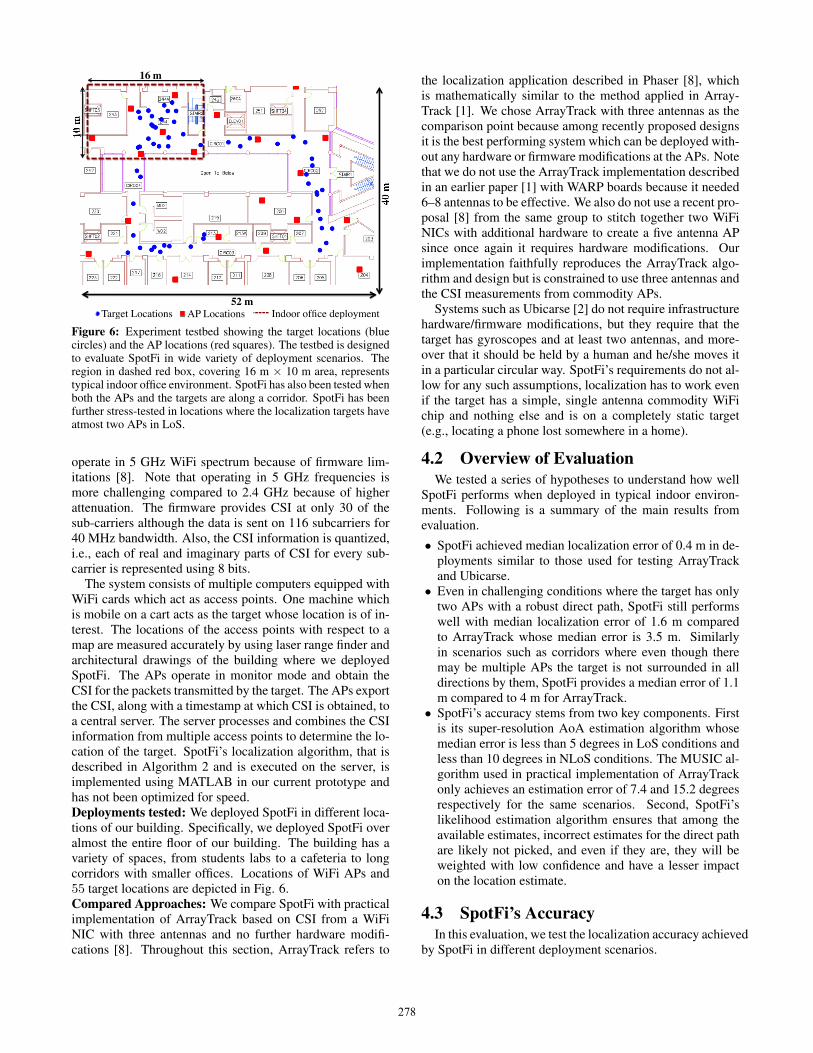
Figure 6: Experiment testbed showing the target locations (bluecircles) and the AP locations (red squares). The testbed is designedto evaluate SpotFi in wide variety of deployment scenarios. Theregion in dashed red box, covering 16 m × 10 m area, representstypical indoor office environment. SpotFi has also been tested whenboth the APs and the targets are along a corridor. SpotFi has beenfurther stress-tested in locations where the localization targets haveatmost two APs in LoS.

operate in 5 GHz WiFi spectrum because of firmware lim-itations [8]. Note that operating in 5 GHz frequencies ismore challenging compared to 2.4 GHz because of higherattenuation. The firmware provides CSI at only 30 of thesub-carriers although the data is sent on 116 subcarriers for40 MHz bandwidth. Also, the CSI information is quantized,i.e., each of real and imaginary parts of CSI for every sub-carrier is represented using 8 bits.

The system consists of multiple computers equipped withWiFi cards which act as access points. One machine whichis mobile on a cart acts as the target whose location is of in-terest. The locations of the access points with respect to amap are measured accurately by using laser range finder andarchitectural drawings of the building where we deployedSpotFi. The APs operate in monitor mode and obtain theCSI for the packets transmitted by the target. The APs exportthe CSI, along with a timestamp at which CSI is obtained, toa central server. The server processes and combines the CSIinformation from multiple access points to determine the lo-cation of the target. SpotFi’s localization algorithm, that isdescribed in Algorithm 2 and is executed on the server, isimplemented using MATLAB in our current prototype andhas not been optimized for speed.Deployments tested: We deployed SpotFi in different loca-tions of our building. Specifically, we deployed SpotFi overalmost the entire floor of our building. The building has avariety of spaces, from students labs to a cafeteria to longcorridors with smaller offices. Locations of WiFi APs and55 target locations are depicted in Fig. 6.Compared Approaches: We compare SpotFi with practicalimplementation of ArrayTrack based on CSI from a WiFiNIC with three antennas and no further hardware modifi-cations [8]. Throughout this section, ArrayTrack refers to

the localization application described in Phaser [8], whichis mathematically similar to the method applied in Array-Track [1]. We chose ArrayTrack with three antennas as thecomparison point because among recently proposed designsit is the best performing system which can be deployed with-out any hardware or firmware modifications at the APs. Notethat we do not use the ArrayTrack implementation describedin an earlier paper [1] with WARP boards because it needed6–8 antennas to be effective. We also do not use a recent pro-posal [8] from the same group to stitch together two WiFiNICs with additional hardware to create a five antenna APsince once again it requires hardware modifications. Ourimplementation faithfully reproduces the ArrayTrack algo-rithm and design but is constrained to use three antennas andthe CSI measurements from commodity APs.

Systems such as Ubicarse [2] do not require infrastructurehardware/firmware modifications, but they require that thetarget has gyroscopes and at least two antennas, and more-over that it should be held by a human and he/she moves itin a particular circular way. SpotFi’s requirements do not al-low for any such assumptions, localization has to work evenif the target has a simple, single antenna commodity WiFichip and nothing else and is on a completely static target(e.g., locating a phone lost somewhere in a home).

4.2 Overview of EvaluationWe tested a series of hypotheses to understand how well

SpotFi performs when deployed in typical indoor environ-ments. Following is a summary of the main results fromevaluation.

• SpotFi achieved median localization error of 0.4 m in de-ployments similar to those used for testing ArrayTrackand Ubicarse.• Even in challenging conditions where the target has only

two APs with a robust direct path, SpotFi still performswell with median localization error of 1.6 m comparedto ArrayTrack whose median error is 3.5 m. Similarlyin scenarios such as corridors where even though theremay be multiple APs the target is not surrounded in alldirections by them, SpotFi provides a median error of 1.1m compared to 4 m for ArrayTrack.• SpotFi’s accuracy stems from two key components. First

is its super-resolution AoA estimation algorithm whosemedian error is less than 5 degrees in LoS conditions andless than 10 degrees in NLoS conditions. The MUSIC al-gorithm used in practical implementation of ArrayTrackonly achieves an estimation error of 7.4 and 15.2 degreesrespectively for the same scenarios. Second, SpotFi’slikelihood estimation algorithm ensures that among theavailable estimates, incorrect estimates for the direct pathare likely not picked, and even if they are, they will beweighted with low confidence and have a lesser impacton the location estimate.

4.3 SpotFi’s AccuracyIn this evaluation, we test the localization accuracy achieved

by SpotFi in different deployment scenarios.

278

0.1 1 100

0.2

0.4

0.6

0.8

1

Localization Error (m)

Em

piri

calC

DF

SpotFiArrayTrack

(a) Indoor office deployment

0.1 1 100

0.2

0.4

0.6

0.8

1

Localization Error (m)

Em

piri

calC

DF

SpotFiArrayTrack

(b) High NLoS deployment

0.1 1 100

0.2

0.4

0.6

0.8

1

Localization Error (m)

Em

piri

calC

DF

SpotFiArrayTrack

(c) Corridors

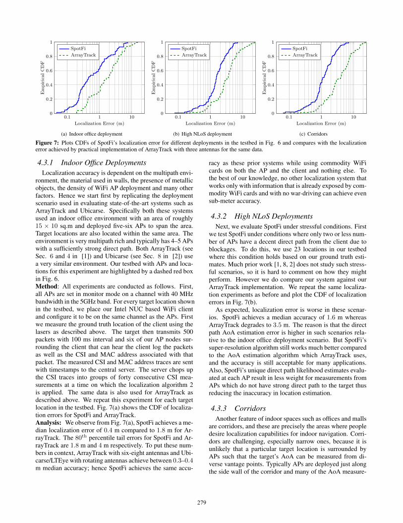
Figure 7: Plots CDFs of SpotFi’s localization error for different deployments in the testbed in Fig. 6 and compares with the localizationerror achieved by practical implementation of ArrayTrack with three antennas for the same data.

4.3.1 Indoor Office DeploymentsLocalization accuracy is dependent on the multipath envi-

ronment, the material used in walls, the presence of metallicobjects, the density of WiFi AP deployment and many otherfactors. Hence we start first by replicating the deploymentscenario used in evaluating state-of-the-art systems such asArrayTrack and Ubicarse. Specifically both these systemsused an indoor office environment with an area of roughly15 × 10 sq.m and deployed five-six APs to span the area.Target locations are also located within the same area. Theenvironment is very multipath rich and typically has 4–5 APswith a sufficiently strong direct path. Both ArrayTrack (seeSec. 6 and 4 in [1]) and Ubicarse (see Sec. 8 in [2]) usea very similar environment. Our testbed with APs and loca-tions for this experiment are highlighted by a dashed red boxin Fig. 6.Method: All experiments are conducted as follows. First,all APs are set in monitor mode on a channel with 40 MHzbandwidth in the 5GHz band. For every target location shownin the testbed, we place our Intel NUC based WiFi clientand configure it to be on the same channel as the APs. Firstwe measure the ground truth location of the client using thelasers as described above. The target then transmits 500packets with 100 ms interval and six of our AP nodes sur-rounding the client that can hear the client log the packetsas well as the CSI and MAC address associated with thatpacket. The measured CSI and MAC address traces are sentwith timestamps to the central server. The server chops upthe CSI traces into groups of forty consecutive CSI mea-surements at a time on which the localization algorithm 2is applied. The same data is also used for ArrayTrack asdescribed above. We repeat this experiment for each targetlocation in the testbed. Fig. 7(a) shows the CDF of localiza-tion errors for SpotFi and ArrayTrack.Analysis: We observe from Fig. 7(a), SpotFi achieves a me-dian localization error of 0.4 m compared to 1.8 m for Ar-rayTrack. The 80th percentile tail errors for SpotFi and Ar-rayTrack are 1.8 m and 4 m respectively. To put these num-bers in context, ArrayTrack with six-eight antennas and Ubi-carse/LTEye with rotating antennas achieve between 0.3–0.4m median accuracy; hence SpotFi achieves the same accu-

racy as these prior systems while using commodity WiFicards on both the AP and the client and nothing else. Tothe best of our knowledge, no other localization system thatworks only with information that is already exposed by com-modity WiFi cards and with no war-driving can achieve evensub-meter accuracy.

4.3.2 High NLoS DeploymentsNext, we evaluate SpotFi under stressful conditions. First

we test SpotFi under conditions where only two or less num-ber of APs have a decent direct path from the client due toblockages. To do this, we use 23 locations in our testbedwhere this condition holds based on our ground truth esti-mates. Much prior work [1, 8, 2] does not study such stress-ful scenarios, so it is hard to comment on how they mightperform. However we do compare our system against ourArrayTrack implementation. We repeat the same localiza-tion experiments as before and plot the CDF of localizationerrors in Fig. 7(b).

As expected, localization error is worse in these scenar-ios. SpotFi achieves a median accuracy of 1.6 m whereasArrayTrack degrades to 3.5 m. The reason is that the directpath AoA estimation error is higher in such scenarios rela-tive to the indoor office deployment scenario. But SpotFi’ssuper-resolution algorithm still works much better comparedto the AoA estimation algorithm which ArrayTrack uses,and the accuracy is still acceptable for many applications.Also, SpotFi’s unique direct path likelihood estimates evalu-ated at each AP result in less weight for measurements fromAPs which do not have strong direct path to the target thusreducing the inaccuracy in location estimation.

4.3.3 CorridorsAnother feature of indoor spaces such as offices and malls

are corridors, and these are precisely the areas where peopledesire localization capabilities for indoor navigation. Corri-dors are challenging, especially narrow ones, because it isunlikely that a particular target location is surrounded byAPs such that the target’s AoA can be measured from di-verse vantage points. Typically APs are deployed just alongthe side wall of the corridor and many of the AoA measure-

279

ments at each AP will be very close to each other due togeometry of the corridors. Also, even if the client has moreAPs in LoS, they are generally farther away than when com-pared to indoor office deployments. This has an importantimplication on localization accuracy since it leads to scenar-ios where many APs have inaccurate and correlated AoAmeasurements and it becomes harder for some AP to correctthe errors of other APs.

We evaluate SpotFi under such a scenario in our testbed.Specifically we look at the target locations in the two cor-ridors that we see in Fig. 6. There are 25 points overallin such locations. We repeat the localization experimentsas described above and compute the localization error forboth SpotFi and ArrayTrack. Again as seen from Fig. 7(c),the median localization error for SpotFi is around a meter,whereas ArrayTrack’s error worsens to 4 m.

Improved localization accuracy of SpotFi is due to twofactors. First, SpotFi resolves multipath more accuratelywith the same number of antennas compared to schemeswhich use only the relative phase information between theantennas. Second, SpotFi’s novel localization algorithm whichaccurately identifies the direct path between the target andthe APs among the estimated multipath components. Wenow test individually the significance of these factors next.

4.4 Deep Dive into SpotFi

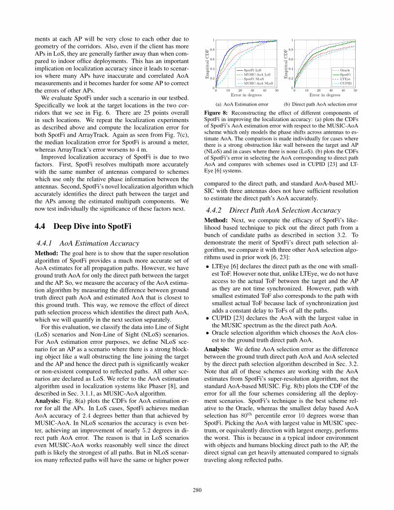
4.4.1 AoA Estimation AccuracyMethod: The goal here is to show that the super-resolutionalgorithm of SpotFi provides a much more accurate set ofAoA estimates for all propagation paths. However, we haveground truth AoA for only the direct path between the targetand the AP. So, we measure the accuracy of the AoA estima-tion algorithm by measuring the difference between groundtruth direct path AoA and estimated AoA that is closest tothis ground truth. This way, we remove the effect of directpath selection process which identifies the direct path AoA,which we will quantify in the next section separately.

For this evaluation, we classify the data into Line of Sight(LoS) scenarios and Non-Line of Sight (NLoS) scenarios.For AoA estimation error purposes, we define NLoS sce-nario for an AP as a scenario where there is a strong block-ing object like a wall obstructing the line joining the targetand the AP and hence the direct path is significantly weakeror non-existent compared to reflected paths. All other sce-narios are declared as LoS. We refer to the AoA estimationalgorithm used in localization systems like Phaser [8], anddescribed in Sec. 3.1.1, as MUSIC-AoA algorithm.Analysis: Fig. 8(a) plots the CDFs for AoA estimation er-ror for all the APs. In LoS cases, SpotFi achieves medianAoA accuracy of 2.4 degrees better than that achieved byMUSIC-AoA. In NLoS scenarios the accuracy is even bet-ter, achieving an improvement of nearly 5.2 degrees in di-rect path AoA error. The reason is that in LoS scenarioseven MUSIC-AoA works reasonably well since the directpath is likely the strongest of all paths. But in NLoS scenar-ios many reflected paths will have the same or higher power

0 10 20 30 40 500

0.2

0.4

0.6

0.8

1

Error in degrees

Empi

rical

CD

F

SpotFi LoSMUSIC-AoA LoSSpotFi NLoSMUSIC-AoA NLoS

(a) AoA Estimation error

0 10 20 30 40 500

0.2

0.4

0.6

0.8

1

Error in degrees

Empi

rical

CD

F

OracleSpotFiLTEyeCUPID

(b) Direct path AoA selection error

Figure 8: Reconstructing the effect of different components ofSpotFi in improving the localization accuracy: (a) plots the CDFsof SpotFi’s AoA estimation error with respect to the MUSIC-AoAscheme which only models the phase shifts across antennas to es-timate AoA. The comparison is made individually for cases wherethere is a strong obstruction like wall between the target and AP(NLoS) and in cases where there is none (LoS). (b) plots the CDFsof SpotFi’s error in selecting the AoA corresponding to direct pathAoA and compares with schemes used in CUPID [23] and LT-Eye [6] systems.

compared to the direct path, and standard AoA-based MU-SIC with three antennas does not have sufficient resolutionto estimate the direct path’s AoA accurately.

4.4.2 Direct Path AoA Selection AccuracyMethod: Next, we compute the efficacy of SpotFi’s like-lihood based technique to pick out the direct path from abunch of candidate paths as described in section 3.2. Todemonstrate the merit of SpotFi’s direct path selection al-gorithm, we compare it with three other AoA selection algo-rithms used in prior work [6, 23]:• LTEye [6] declares the direct path as the one with small-

est ToF. However note that, unlike LTEye, we do not haveaccess to the actual ToF between the target and the APas they are not time synchronized. However, path withsmallest estimated ToF also corresponds to the path withsmallest actual ToF because lack of synchronization justadds a constant delay to ToFs of all the paths.• CUPID [23] declares the AoA with the largest value in

the MUSIC spectrum as the the direct path AoA.• Oracle selection algorithm which chooses the AoA clos-

est to the ground truth direct path AoA.Analysis: We define AoA selection error as the differencebetween the ground truth direct path AoA and AoA selectedby the direct path selection algorithm described in Sec. 3.2.Note that all of these schemes are working with the AoAestimates from SpotFi’s super-resolution algorithm, not thestandard AoA-based MUSIC. Fig. 8(b) plots the CDF of theerror for all the four schemes considering all the deploy-ment scenarios. SpotFi’s technique is the best scheme rel-ative to the Oracle, whereas the smallest delay based AoAselection has 80th percentile error 10 degrees worse thanSpotFi. Picking the AoA with largest value in MUSIC spec-trum, or equivalently direction with largest energy, performsthe worst. This is because in a typical indoor environmentwith objects and humans blocking direct path to the AP, thedirect signal can get heavily attenuated compared to signalstraveling along reflected paths.

280

0.1 1 100

0.2

0.4

0.6

0.8

1

Localization error (m)

Empi

rical

CD

F3 APs4 APs5 APs

(a) localization error with differentAP densities

0.1 1 100

0.2

0.4

0.6

0.8

1

Localization Error (m)

Empi

rical

CD

F

6 Pkts10 Pkts40 Pkts

(b) localization error with differentnumber of packets used for

localization

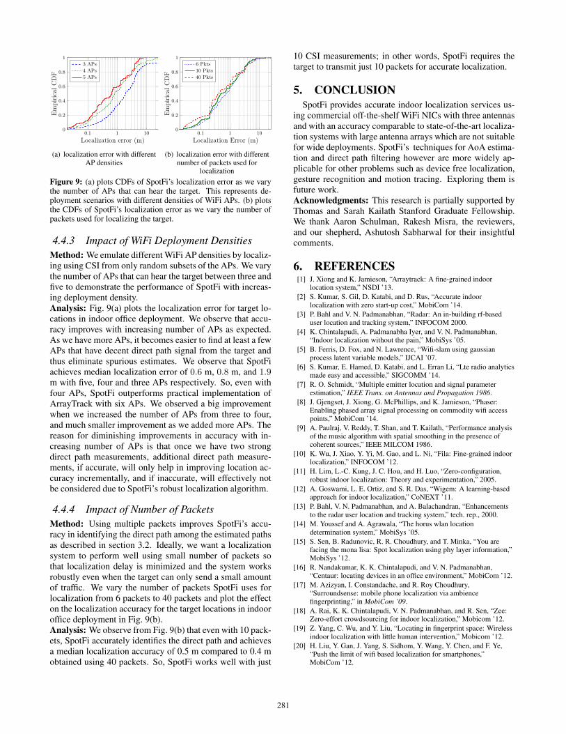
Figure 9: (a) plots CDFs of SpotFi’s localization error as we varythe number of APs that can hear the target. This represents de-ployment scenarios with different densities of WiFi APs. (b) plotsthe CDFs of SpotFi’s localization error as we vary the number ofpackets used for localizing the target.

4.4.3 Impact of WiFi Deployment DensitiesMethod: We emulate different WiFi AP densities by localiz-ing using CSI from only random subsets of the APs. We varythe number of APs that can hear the target between three andfive to demonstrate the performance of SpotFi with increas-ing deployment density.Analysis: Fig. 9(a) plots the localization error for target lo-cations in indoor office deployment. We observe that accu-racy improves with increasing number of APs as expected.As we have more APs, it becomes easier to find at least a fewAPs that have decent direct path signal from the target andthus eliminate spurious estimates. We observe that SpotFiachieves median localization error of 0.6 m, 0.8 m, and 1.9m with five, four and three APs respectively. So, even withfour APs, SpotFi outperforms practical implementation ofArrayTrack with six APs. We observed a big improvementwhen we increased the number of APs from three to four,and much smaller improvement as we added more APs. Thereason for diminishing improvements in accuracy with in-creasing number of APs is that once we have two strongdirect path measurements, additional direct path measure-ments, if accurate, will only help in improving location ac-curacy incrementally, and if inaccurate, will effectively notbe considered due to SpotFi’s robust localization algorithm.

4.4.4 Impact of Number of PacketsMethod: Using multiple packets improves SpotFi’s accu-racy in identifying the direct path among the estimated pathsas described in section 3.2. Ideally, we want a localizationsystem to perform well using small number of packets sothat localization delay is minimized and the system worksrobustly even when the target can only send a small amountof traffic. We vary the number of packets SpotFi uses forlocalization from 6 packets to 40 packets and plot the effecton the localization accuracy for the target locations in indooroffice deployment in Fig. 9(b).Analysis: We observe from Fig. 9(b) that even with 10 pack-ets, SpotFi accurately identifies the direct path and achievesa median localization accuracy of 0.5 m compared to 0.4 mobtained using 40 packets. So, SpotFi works well with just

10 CSI measurements; in other words, SpotFi requires thetarget to transmit just 10 packets for accurate localization.

5. CONCLUSIONSpotFi provides accurate indoor localization services us-

ing commercial off-the-shelf WiFi NICs with three antennasand with an accuracy comparable to state-of-the-art localiza-tion systems with large antenna arrays which are not suitablefor wide deployments. SpotFi’s techniques for AoA estima-tion and direct path filtering however are more widely ap-plicable for other problems such as device free localization,gesture recognition and motion tracing. Exploring them isfuture work.Acknowledgments: This research is partially supported byThomas and Sarah Kailath Stanford Graduate Fellowship.We thank Aaron Schulman, Rakesh Misra, the reviewers,and our shepherd, Ashutosh Sabharwal for their insightfulcomments.

6. REFERENCES[1] J. Xiong and K. Jamieson, “Arraytrack: A fine-grained indoor

location system,” NSDI ’13.[2] S. Kumar, S. Gil, D. Katabi, and D. Rus, “Accurate indoor

localization with zero start-up cost,” MobiCom ’14.[3] P. Bahl and V. N. Padmanabhan, “Radar: An in-building rf-based

user location and tracking system,” INFOCOM 2000.[4] K. Chintalapudi, A. Padmanabha Iyer, and V. N. Padmanabhan,

“Indoor localization without the pain,” MobiSys ’05.[5] B. Ferris, D. Fox, and N. Lawrence, “Wifi-slam using gaussian

process latent variable models,” IJCAI ’07.[6] S. Kumar, E. Hamed, D. Katabi, and L. Erran Li, “Lte radio analytics

made easy and accessible,” SIGCOMM ’14.[7] R. O. Schmidt, “Multiple emitter location and signal parameter

estimation,” IEEE Trans. on Antennas and Propagation 1986.[8] J. Gjengset, J. Xiong, G. McPhillips, and K. Jamieson, “Phaser:

Enabling phased array signal processing on commodity wifi accesspoints,” MobiCom ’14.

[9] A. Paulraj, V. Reddy, T. Shan, and T. Kailath, “Performance analysisof the music algorithm with spatial smoothing in the presence ofcoherent sources,” IEEE MILCOM 1986.

[10] K. Wu, J. Xiao, Y. Yi, M. Gao, and L. Ni, “Fila: Fine-grained indoorlocalization,” INFOCOM ’12.

[11] H. Lim, L.-C. Kung, J. C. Hou, and H. Luo, “Zero-configuration,robust indoor localization: Theory and experimentation,” 2005.

[12] A. Goswami, L. E. Ortiz, and S. R. Das, “Wigem: A learning-basedapproach for indoor localization,” CoNEXT ’11.

[13] P. Bahl, V. N. Padmanabhan, and A. Balachandran, “Enhancementsto the radar user location and tracking system,” tech. rep., 2000.

[14] M. Youssef and A. Agrawala, “The horus wlan locationdetermination system,” MobiSys ’05.

[15] S. Sen, B. Radunovic, R. R. Choudhury, and T. Minka, “You arefacing the mona lisa: Spot localization using phy layer information,”MobiSys ’12.

[16] R. Nandakumar, K. K. Chintalapudi, and V. N. Padmanabhan,“Centaur: locating devices in an office environment,” MobiCom ’12.

[17] M. Azizyan, I. Constandache, and R. Roy Choudhury,“Surroundsense: mobile phone localization via ambiencefingerprinting,” in MobiCom ’09.

[18] A. Rai, K. K. Chintalapudi, V. N. Padmanabhan, and R. Sen, “Zee:Zero-effort crowdsourcing for indoor localization,” Mobicom ’12.

[19] Z. Yang, C. Wu, and Y. Liu, “Locating in fingerprint space: Wirelessindoor localization with little human intervention,” Mobicom ’12.

[20] H. Liu, Y. Gan, J. Yang, S. Sidhom, Y. Wang, Y. Chen, and F. Ye,“Push the limit of wifi based localization for smartphones,”MobiCom ’12.

281

[21] H. Wang, S. Sen, A. Elgohary, M. Farid, M. Youssef, and R. R.Choudhury, “No need to war-drive: unsupervised indoorlocalization,” MobiSys ’12.

[22] M. Youssef and A. Agrawala, “Small-scale compensation for wlanlocation determination systems,” in IEEE Wireless Communicationsand Networking, 2003.

[23] S. Sen, J. Lee, K.-H. Kim, and P. Congdon, “Avoiding multipath torevive inbuilding wifi localization,” MobiSys ’13.

[24] K. Joshi, S. Hong, and S. Katti, “Pinpoint: localizing interferingradios,” NSDI ’13.

[25] D. Niculescu and B. Nath, “Vor base stations for indoor 802.11positioning,” MobiCom ’04.

[26] L. Atzori, A. Iera, and G. Morabito, “The internet of things: Asurvey,” Comput. Netw. ’10.

[27] P. Chen, P. Ahammad, C. Boyer, S. i Huang, L. Lin, E. Lobaton,M. Meingast, S. Oh, S. Wang, P. Yan, A. Y. Yang, C. Yeo, L. chungChang, J. D. Tygar, and S. S. Sastry, “Citric: A low-bandwidthwireless camera network platform,” ICDSC ’08.

[28] nest. https://nest.com/.[29] M. Youssef, A. Youssef, C. Rieger, U. Shankar, and A. Agrawala,

“Pinpoint: An asynchronous time-based location determinationsystem,” MobiCom ’06.

[30] S. A. Golden and S. S. Bateman, “Sensor measurements for wi-filocation with emphasis on time-of-arrival ranging,” IEEE Trans. onMobile Computing, 2007.

[31] A. T. Mariakakis, S. Sen, J. Lee, and K.-H. Kim, “Sail: Single accesspoint-based indoor localization,” MobiCom ’14.

[32] A. Marcaletti, M. Rea, D. Giustiniano, V. Lenders, andA. Fakhreddine, “Filtering noisy 802.11 time-of-flight rangingmeasurements,” CoNEXT ’14.

[33] M. Ciurana, F. Barcelo-Arroyo, and F. Izquierdo, “A ranging systemwith ieee 802.11 data frames,” in IEEE Radio and WirelessSymposium, 2007.

[34] S. Lanzisera, D. Zats, and K. S. Pister, “Radio frequencytime-of-flight distance measurement for low-cost wireless sensorlocalization,” IEEE Sensors Journal, 2011.

[35] J. Xiong, K. Jamieson, and K. Sundaresan, “Synchronicity: Pushingthe envelope of fine-grained localization with distributed mimo,”HotWireless ’14.

[36] F. Zhao, W. Yao, C. C. Logothetis, and Y. Song, “Super-resolutiontoa estimation in ofdm systems for indoor environments,” in IEEEInternational Conference on Networking, Sensing and Control, 2007.

[37] V. Amendolare, D. Cyganski, and R. J. Duckworth, “Transactionalarray reconciliation tomography for precision indoor location,” IEEETrans. on Aerospace and Electronic Systems, 2014.

[38] S. Venkatraman and J. Caffery, “Hybrid toa/aoa techniques formobile location in non-line-of-sight environments,” in IEEE WirelessCommunications and Networking Conference, 2004.

[39] A. Cavanaugh, M. Lowe, D. Cyganski, and R. Duckworth, “Wpiprecision personnel location system: Rapid deployment antennasystem and sensor fusion for 3d precision location,” in Institute ofNavigation-International Technical Meeting 2010.

[40] H. Rahul, H. Hassanieh, and D. Katabi, “Sourcesync: a distributedwireless architecture for exploiting sender diversity,” ACMSIGCOMM CCR ’11.

[41] M. Wax and A. Leshem, “Joint estimation of time delays anddirections of arrival of multiple reflections of a known signal,” IEEEICASSP 1996.

[42] A.-J. Van Der Veen, M. C. Vanderveen, and A. J. Paulraj, “Jointangle and delay estimation using shift-invariance properties,” IEEESignal Processing Letters 1997.

[43] M. C. Vanderveen, A.-J. Van der Veen, and A. Paulraj, “Estimationof multipath parameters in wireless communications,” IEEE Trans.on Signal Processing 1998.

[44] M. Vanderveen, B. Ng, C. Papadias, and A. Paulraj, “Joint angle anddelay estimation (jade) for signals in multipath environments,” inConference Record of the Thirtieth Asilomar Conference on Signals,Systems and Computers, 1996.

[45] Y.-Y. Wang, J.-T. Chen, and W.-H. Fang, “Tst-music for jointdoa-delay estimation,” IEEE Trans. on Signal Processing, 2001.

[46] J. Picheral and U. Spagnolini, “Shift invariance algorithms for theangle/delay estimation of multipath space-time channel,” inVehicular Technology Conference, 2001.

[47] D. Inserra and A. M. Tonello, “A frequency-domain losangle-of-arrival estimation approach in multipath channels,” IEEETrans. on Vehicular Technology, 2013.

[48] J.-T. Chen, J. Kim, and J.-W. Liang, “Multichannel mlse equalizerwith parametric fir channel identification,” IEEE Trans. on VehicularTechnology, 1999.

[49] G. G. Raleigh and T. Boros, “Joint space-time parameter estimationfor wireless communication channels,” IEEE Trans. on SignalProcessing, 1998.

[50] J. He, M. Swamy, and M. O. Ahmad, “Joint space-time parameterestimation for underwater communication channels with velocityvector sensor arrays,” IEEE Trans. on Wireless Communications, ’12.

[51] H. Yamada, M. Ohmiya, Y. Ogawa, and K. Itoh, “Superresolutiontechniques for time-domain measurements with a network analyzer,”IEEE Trans. on Antennas and Propagation, 1991.

[52] M. Ascione, A. Buonanno, M. D’Urso, L. Angrisani, and R. SchianoLo Moriello, “A new measurement method based on music algorithmfor through-the-wall detection of life signs,” IEEE Trans. onInstrumentation and Measurement, 2013.

[53] J. Wang, F. Adib, R. Knepper, D. Katabi, and D. Rus, “Rf-compass:robot object manipulation using rfids,” MobiCom ’13.

[54] J. Wang and D. Katabi, “Dude, where’s my card?: Rfid positioningthat works with multipath and non-line of sight,” in ACM SIGCOMMCCR ’13.

[55] J. Wang, D. Vasisht, and D. Katabi, “Rf-idraw: Virtual touch screenin the air using rf signals,” SIGCOMM ’14.

[56] S. Gezici, Z. Tian, G. B. Giannakis, H. Kobayashi, A. F. Molisch,H. V. Poor, and Z. Sahinoglu, “Localization via ultra-widebandradios: a look at positioning aspects for future sensor networks,”IEEE Signal Processing Magazine, 2005.

[57] A. Ward, A. Jones, and A. Hopper, “A new location technique for theactive office,” IEEE Personal Communications, 1997.

[58] R. K. Harle and A. Hopper, “Deploying and evaluating alocation-aware system,” MobiSys ’05.

[59] N. B. Priyantha, A. Chakraborty, and H. Balakrishnan, “The cricketlocation-support system,” MobiCom 2000.

[60] A. Harter, A. Hopper, P. Steggles, A. Ward, and P. Webster, “Theanatomy of a context-aware application,” Wireless Networks, 2002.

[61] A. Savvides, C.-C. Han, and M. B. Strivastava, “Dynamic fine-grained localization in ad-hoc networks of sensors,” MobiCom ’01.

[62] R. Want, A. Hopper, V. Falcao, and J. Gibbons, “The active badgelocation system,”

[63] A. Harter and A. Hopper, “A distributed location system for theactive office,” IEEE Network, 1994.

[64] E. Aitenbichler and M. Muhlhauser, “An ir local positioning systemfor smart items and devices,” in Distributed Computing SystemsWorkshops, 2003.

[65] P. Hu, L. Li, C. Peng, G. Shen, and F. Zhao, “Pharos: Enable physicalanalytics through visible light based indoor localization,” HotNets’13.

[66] Y.-S. Kuo, P. Pannuto, K.-J. Hsiao, and P. Dutta, “Luxapose: Indoorpositioning with mobile phones and visible light,” MobiCom ’14.

[67] iBeacon. https://developer.apple.com/ibeacon/.[68] D. Halperin, W. Hu, A. Sheth, and D. Wetherall, “Tool release:

Gathering 802.11n traces with channel state information,” ACMSIGCOMM CCR ’11.

[69] N. Czink, M. Herdin, H. Ozcelik, and E. Bonek, “Number ofmultipath clusters in indoor mimo propagation environments,”Electronics Letters ’04.

[70] V. Erceg, L. Schumacher, P. Kyritsi, and et al, “Tgn channel models,”Tech. Rep. IEEE P802.11, Wireless LANs, 2004.

[71] A. Goldsmith, Wireless communications. Cambridge university press,2005.

[72] S. Boyd and L. Vandenberghe, Convex Optimization. New York, NY,USA: Cambridge University Press, 2004.

282