Embed Size (px)
Citation preview
PHYSICAL REVIEW A VOLUME 33, NUMBER 6 JUNE 1986
Spontaneous symmetry breaking and neutral stability in the noncanonical Hamiltonian formalism
P. J. Morrison Institute for Fusion Studies and Department of Physics, The University of Texas at Austin, Austin, Texas 78712
S. Eliezer* Institute for Fusion Studies, The University of Texas at Austin, Austin, Texas 78712
(Received 25 November 1985)
The noncanonical Hamiltonian formalism is based upon a generalization of the Poisson bracket, a particular form of which is possessed by continuous media fields. Associated with this generalization are special constants of motion called Casimir invariants. These are constants that can be viewed as being built into the phase space, for they are invariant for all Hamiltonians. Casimir invariants are important because when added to the Hamiltonian they yield an effective Hamiltonian that produces equilibrium states upon variation. The stability of these states can be ascertained by a second variation. Goldstone's theorem, in its usual context, determines zero eigenvalues of the mass matrix for a given vacuum state, the equilibrium with minimum energy. Here, since for fluids and plasmas the vacuum state is uninteresting, we examine symmetry breaking for general equilibria. Broken symmetries imply directions of neutral stability. Two examples are presented: the nonlinear Alfven wave of plasma physics and the Korteweg-de Vries soliton.
I. INTRODUCTION
The notion of spontaneous symmetry breaking is an essential idea in relativistic field-theoretic models that describe the electromagnetic, weak, and strong interactions. I Spontaneous symmetry breaking occurs when the vacuum state of a physical system possesses less symmetry than its Lagrangian. For scalar fields Goldstone's theorem2- 4 tells us that corresponding to each broken continuous symmetry there is a massless boson. Alternatively, for nonrelativistic many-body quantum systems such as superfluids, superconductors, and ferromagnets, spontaneous symmetry breaking is related to excitation branches that do not have an energy gap. S In a classical physics sense one can interpret these phenomena as arising from a particular energy functional for which the vacuum state is not an isolated minimum but possesses directions of neutral stability. It is this general feature that we grasp here in order to investigate spontaneous symmetry breaking for fields, such as continuous-media fields in the Eulerian-variable representation that describe fluids and plasmas.
Field theories are usually described by means of the action-functional formalism or its corresponding canonical Hamiltonian description. Here we depart from this and describe spontaneous symmetry breaking in what has been called the generalized or noncanonical Hamiltonian formalism. This is the natural setting for continuousmedia fields that are written in terms of the usual physical Eulerian variables. The basic object of the noncanonical Hamiltonian formalism is the Poisson bracket, which is generalized. The emphasis is placed on the Lie algebraic properties of the bracket rather than on the usual specific canonical form. Consequently, the bracket may
33
have dependence upon the field variables, contain operators, and possess degeneracy. For continuous media there is a generic form that is earmarked by linear dependence upon the field variables in conjunction with operators that are structure operators for a Lie algebra. Whether or not the bracket is of this generic form, associated with degeneracy are special constants of motion called Casimir invariants. These are constants that can be viewed as being built into phase space, for they have vanishing Poisson bracket with all Hamiltonians. Casimir invariants play an important role in the noncanonical formalism and its application to spontaneous symmetry breaking.
The spontaneous breaking of symmetry can be observed in either the Lagrangian or the Hamiltonian pictures. In both cases the vacuum state corresponds to a minimum of the potential energy functional. For the noncanonical Hamiltonian formalism treated here, equilibria of a field theory correspond to extremals of a functional composed of the Hamiltonian plus Casimir invariants. The second variation of this functional can be used to ascertain the stability of an equilibrium. In this paper we draw a parallel between the conventional vacuum state, which is an absolute minimum of the potential energy functional although not necessarily an isolated point, and an equilibrium of a noncanonical field theory, which may be a nonisolated relative extremum. We thus observe a parallel between the conventional mass matrix and the second variation of our functional. Zero-mass particles of the former are analogous to neutral directions of the latter. Broken symmetries of our functional result in such neutral directions.
We organize this paper by first briefly reviewing the noncanonical Hamiltonian formalism, then by discussing stability, symmetry breaking, and examples, before con-
4205 © 1986 The American Physical Society
4206 P. J. MORRISON AND S. ELIEZER 33
cluding. In Sec. II finite-degree-of-freedom systems are treated. This material has a long history that includes work motivated by Lie, Dirac, and others. For greater depth we recommend Ref. 6 for a coordinate approach and Ref. 7 (and references therein) for a modern geometrical slant. A readable exposition is given in Ref. 8. In Sec. III we discuss field theories. The reader may find Refs. 9 and 10 helpful. Section IV deals with stability. Criteria for null eigenvalues and eigenvectors are obtained. In Sec. V symmetry breaking is described and generalized to include noncanonical Hamiltonian fields. Applications are discussed in Sec. VI. In particular, the nonlinear Alfven wave of plasma physics, and the Korteweg-de Vries soliton are treated. We conclude in Sec. VII.
II. NONCANONICAL HAMILTONIAN MECHANICS
The canonical method for obtaining Hamilton's equations of motion is to start by identifying the configuration space and then through physical considerations write down the Lagrangian
L(q,q)=T- V. (2.1)
Here the configuration-space coordinates are q=(ql, ... ,qN) with corresponding velocities q=(ql>'" ,qN); T and V are the usual kinetic and potential energies. Variation of the Lagrangian (2.1) yields the Euler-Lagrange equations of motion, from which Hamilton's equations are obtained by a Legendre transformation. The Hamiltonian H is given by
N
H(q,p)= l: Pkqk-L(q,q), (2.2) k=1
where the canonical momenta Pk are defined by
aL Pk=-.-, k =1, ... ,N .
aqk (2.3)
Hamilton's equations in canonical form are conveniently written as
qj = aaH =[qj,H] , 'PI
P; = - aaH =[pj,H], i = 1, ... ,N qj
where the Poisson bracket is defined by
[j,g]= f [-2L..EL_-2L..EL 1 ' k = I aqk apk apk aqk
(2.4)
(2.5)
and j and g are functions of the phase-space variables (q,p). Alternately, one can define the phase space by zj=qj for i=I, ... ,N and zj=Pi-N for i =N + I,N +2, ... ,2N. Using Zi, the Poisson bracket becomes
where
(Jji)= [ 0 -IN
(2.6)
(2.7)
is a 2NX2N matrix and IN is the NXN unit matrix. (Here and henceforth we sum repeated indices.) The quantity (Jii) is a second-order contravariant tensor that is called the cosymplectic form. It is the dual or inverse of the symplectic two-form that is sometimes taken as the starting point for defining Hamiltonian flows. Hamilton's equations in this representation are
i i=[ZI,H]=Jli aH . (2.8) azi
It is not always possible to obtain Eqs. (2.8) by the procedure described above because the Legendre transformation may not exist. When this occurs one must employ Dirac constraint theory.6.11-13 This theory leads one to Poisson brackets that are not of the standard form, the so-called Dirac brackets. Also, brackets of nonstandard form arise by the process of reductionl4•15 where the dimension of a phase space is decreased by virtue of certain symmetries in a Hamiltonian. Here we are not concerned with this passage from degenerate Lagrangians to Dirac brackets or with reduction, but rather we emphasize a generalization of the Poisson bracket that includes both.
Canonical transformations, by definition, preserve the form of the Poisson bracket, but an arbitrary coordinate transformation does not and thus in this case the form of Hamilton's equations can be obscured. However, in spite of the obscured form in the latter case, the important algebraic properties, such as bilinearity, antisymmetry, and the Jacobi identity conditions of the Poisson bracket, are maintained. This motivates the following definition of the generalized or noncanical Hamiltonian formalism: a system is Hamiltonian in this sense if one can find a Poisson bracket with the appropriate algebraic properties and a Hamiltonian which generates the time evolution of the system. The formalism can be cast in the following form:
'j J-ijaH . 1 M Z= -.,1= , ... , , azJ
(2.9)
where aii) need not have the form of Eq. (2.7). It may depend explicitly on zi, and the number of coordinates M defining the phase space need not be even. The M X M matrix a ii) defines the Poisson bracket in analogy to Eq. (2.6),
(f,g]=~Jii ago . (2.10) az' azJ
This generalized Poisson bracket allows for special constants C, called Casimir invariants, which commute with the Hamiltonian as well as with any function F of the dynamical variables Zi describing the system, i.e.,
[C,F(z)] =0 . (2.11)
A consequence of this definition of the Casimir invariants, using Eq. (2.10), is
ac: Jii a~ =0 , (2.12) az' azJ
but F is arbitrary and therefore
Jii ac, = 0 . 1 M azJ ,I = , ... , . (2.13)
33 SPONTANEOUS SYMMETRY BREAKING AND NEUTRAL ... 4207
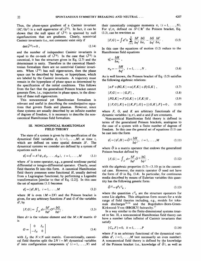
Thus, the phase-space gradient of a Casimir invariant (aC laz i ) is a null eigenvector of a Ii). In fact, it can be shown that the null space of ail) is spanned by null eigenfunctions that are gradients. Clearly, nontrivial Casimir invariants (Le., not constants) exist only if
(2.14)
and the number of independent Casimir invariants is equal to the co-rank of ali). In the case that (Jil) is canonical, it has the structure given in Eq. (2.7) and the determinant is unity. Therefore in the canonical Hamiltonian formalism there are no nontrivial Casimir invariants. When (Jii) has null eigenvectors, then the phase space can be described by leaves, or hyperplanes, which are labeled by the Casimir invariants. A trajectory must remain in the hyperplane of phase space as determined by the specification of the initial conditions. This follows from the fact that the generalized Poisson bracket cannot generate flow, i.e., trajectories in phase space, in the direction of these null eigenvectors.
This noncanonical yet Hamiltonian formalism is relevant and useful in describing the nondissipative equations that govern fluids and plasmas. However, since these systems are usually described by an infinite number of degrees of freedom, it is necessary to describe the noncanonical Hamiltonian field formalism.
III. NONCANONICAL HAMILTONIAN FIELD THEORY
The state of a system is given by the specification of the dynamical field variables 1/JI (i = 1, ... ,M) at time t, which are defined on some spatial domain ~. The dynamical systems we consider are defined by a system of equations such as
. -i . 1/J~=1/J=A'(1/JI,1/J2, ... ,1/JM)' i=I, ... ,M (3.1)
where A I is some operator, e.g., a general nonlinear partial differential or integro-differential operator. Clearly, usual field theories fit into this form. A canonical Hamiltonian field theory possesses some functional H, usually derived from a Lagrangian functional, by performing a Legendre transformation [similar to that of Eq. (2.2)]. In this case the set of equations (3.1) becomes
tfr={1/Ji,Hj, i=I, ... ,M (3.2)
where M is even (M = 2N) and the Poisson bracket is given, for any arbitrary functions F and G of the variables ~,by
{F Gj = f dT BF.Oji BG .. , !'R B1/J' B1/JJ
(3.3)
Here dT is the volume element and the MXM matrix 0 is
(3.4)
with IN the NXN unit matrix. Conventionally, canonical field theories split the 2N ( = M) dynamical variables ~ into configuration components r/ (i = 1, ... , N) and
their canonically conjugate momenta 1Tj (i = 1, ... ,N). For r/,1TI defined on ~ CR3 the Poisson bracket, Eq. (3.3), can be rewritten as
{F,Gj = f d 3x f B~ BG _ BG. BF . (3.5) 1=1 B'TJ' B1Ti B'TJ' B1Ti
In this case the equations of motion (3.2) reduce to the Hamiltonian field equations
BH 'TJI __ -r- B1T1 '
aH 1Tit=- B'TJI ' i=I, ... ,N. (3.6)
As is well known, the Poisson bracket of Eq. (3.5) satisfies the following algebraic relations:
[aF+pG,Kj =a[F,Kj +P[G,Kj , (3.7)
{F,Gj=-{G,Fj, (3.8)
{FG,Kj=F{G,Kj+{F,KjG, (3.9)
{{ F,Gj,K} + ({K,Fj,G} + {{G,Kj,F} =0, (3.10)
where F, G, and K are arbitrary functionals of the dynamic variables ('TJ, 1T), and a and P are constants.
Noncanonical Hamiltonian field theory is defined in terms of the generalized Poisson brackets, analogous to the case of a system with a finite number of degrees of freedom. In this case the general set of equations (3.1) can be cast into the form
. . -··BH 1/J~={"",HJ=O'J-., i=I, ... ,M (3.11)
B1/JJ
where (5 is a matrix operator that endows the generalized Poisson bracket defined by
{ F G I = f dT BF. i5 Ii BG , !i" B1/J' 81/J J '
(3.12)
with the algebraic properties (3.7)-(3.10) as in the canonical case. However, the matrix operator (5 need not have the form of 0 in Eq. (3.4). In particular, for continuous media described by means of Eulerian variables this quantity has the following generic form:
(3.13)
where the quantities Ciik are the structure operators for some Lie algebra. This Ubiquitous form occurs for a wide range of field theories including, e.g., models for tokamak discharges 10, 16 and the Bogoliubov-Born-GreenKirkwood-Yvon (BBGKY) heirarchyY
In a way similar to the finite-dimensional systems treated in Sec. II, a noncanonical Hamiltonian field theory can have a number (often infinite) of Casimir invariants that satisfy
{Ck,Fj =0, k =1, ... ,P (3.14)
where F is an arbitrary functional of the dynamical variables ~, i = 1, ... ,M (not necessarily an even number). A noncanonical field theory is defined by the knowledge of the Poisson bracket (i.e., knowledge of (5), as well as
4208 P. J. MORRISON AND S. ELIEZER 33
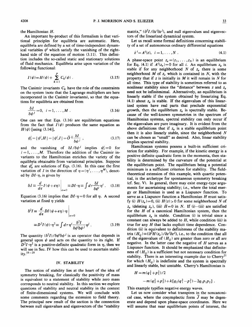
the Hamiltonian H. An important by-product of this fonnalism is that vari
tional principles for equilibria are automatic. Here, equilibria are defined by a set of time-independent dynamical variables t/Ji which satisfy the vanishing of the righthand side of the equation of motion (3.11). This definition includes the so-called static and stationary solutions of fluid mechanics. Equilibria arise upon variation of the following functional:
p
1(t/J)=H(t/J)+ :I Ck(t/J) . (3.15) k=l
The Casimir invariants Ck have the role of the constraints on the system (note that the Lagrange multipliers are here incorporated in the Casimir invariants), so that the equations for equilibria are obtained from
81. =0, i = 1, ... ,M . (3.16) 8t/Jl
One can see that Eqs. (3.16) are equilibrium equations from the fact that I (t/J) produces the same equation as H(t/J) [using (3.14)],
t/J~= I t/Ji,HJ = I t/Ji,lJ =0 ij 81. , (3.17) 8t/Jl
and the vanishing of 81 18t/Jj implies t/J~ =0 for i = 1, ... ,M. Therefore the addition of the Casimir invariants to the Hamiltonian enriches the variety of the equilibria obtainable from variational principles. Suppose that vie are solutions of Eqs. (3.16). In this case the first variation of I in the direction of 1/=(1/1, ... ,1/M), denoted by Dl'1/, is given by
d I J 81 . 81= -1(t/J+E1/) =Dl'1/= d-r-.1/'. (3.18) dE E=O 8t/J'
Equation (3.16) implies that Dl'1/=O for all 1/. variation at fixed 1/ yields
821= dd Dl(t/J+E1/)'1/1 E E=O
2 2 J . 821 . =D 1(t/J)'1/ = d-r1/'-.-.1l'. 8t/J'8t/Jl
A second
(3.19)
The quantity (821)/8t/Ji8t/Jj is an operator that depends in general upon t/J and acts on the quantity to its right. If D 21'1/2 is a positive-definite quadratic fonn in 1/, then we will see in Sec. IV how this can be used to ascertain stability.18-20
IV. STABILITY
The notion of stability lies at the heart of the idea of symmetry breaking, for classically the positivity of mass is equivalent to a statement of stability while zero mass corresponds to neutral stability. In this section we explore questions of stability and neutral stability in the context of finite-dimensional systems. We will conclude with some comments regarding the extension to field theory. The principal new result of the section is the connection between null eigenvalues and eigenvectors of the "stability
matrix," (a21Iaziazj ), and null eigenvalues and eigenvectors of the linearized dynamical system.
Let us recall some fonnal definitions concerning stability of a set of autonomous ordinary differential equations
(4.1)
A phase-space point ze=(z\t ... ,ZN) is an equilibrium for Eq. (4.1) if Ai(ze)=O for all i. An equilibrium Ze is stable if for any neighborhood N of Ze there is some neighborhood M of Ze which is contained in N, with the property that if Z is initially in M it will remain in N for all time. This type of stability is sometimes referred to as nonlinear stability since the "distance" between Z and Ze
need not be infinitesimal. Alternatively, an equilibrium is linearly stable if the system obtained by linearizing Eq. (4.1) about Ze is stable. If the eigenvalues of this linearized system have real parts that preclude exponential growth, then the equilibrium Ze is spectrally stable. Because of the well-known symmetries in the spectrum of Hamiltonian systems, spectral stability can only occur if the eigenvalues are pure imaginary. It is evident from the above definitions that if Ze is a stable equilibrium point then it is also linearly stable, since the neighborhood N can be chosen as "small" as desired. Also, linear stability implies spectral stability.
Hamiltonian systems possess a built-in sufficient criterion for stability. For example, if the kinetic energy is a positive definite quadratic fonn in the momenta, then stability is detennined by the curvature of the potential at the equilibrium point. The equilibrium being a potential minimum is a sufficient criterion for stability. The fieldtheoretical extension of this example, with quartic potential, is the archetype for spontaneous symmetry breaking (cf. Sec. V). In general, there may exist energy-type arguments for ascertaining stability; i.e., where the total energy or Hamiltonian is used as a Liapunov function. To serve as a Liapunov function a Hamiltonian H must satisfy (i) H (ze ) = 0, (ii) H (z) > 0 for some neighborhood N of Ze (deleting ze), (iii) if = 0 in N. If (i)-Wi) are satisfied for the H of a canonical Hamiltonian system, then the equilibrium Ze is stable. Condition (i) is trivial since a constant can always be added to H, while condition (iii) is true for any H that lacks explicit time dependence. Condition (ii) is equivalent to definiteness of the stability matrix (Hij)=(a2H(ze)/aziazi), i.e., to the condition that all of the eigenvalues of (Hij ) are greater than zero or all are negative. In the latter case the negative of H serves as a Liapunov function. It should be emphasized that definiteness of (Hii ) is a sufficient but not necessary condition for stability. There is an interesting example due to Cherry21 for which (Hij ) is indefinite and the system is spectrally and linearly stable, but unstable. Cherry's Hamiltonian is
H=m(qI+PI)/2
-m(q~+p~)+k[q2(qr-pr)-2qlpIP2] .
This example typifies negative energy waves. Let us now consider what transpires in the noncartoni
cal case, where the cosymplectic fonn J may be degenerate and depend upon phase-space coordinates. Here we will assume that near equilibrium points of interest, the
33 SPONTANEOUS SYMMETRY BREAKING AND NEUTRAL ... 4209
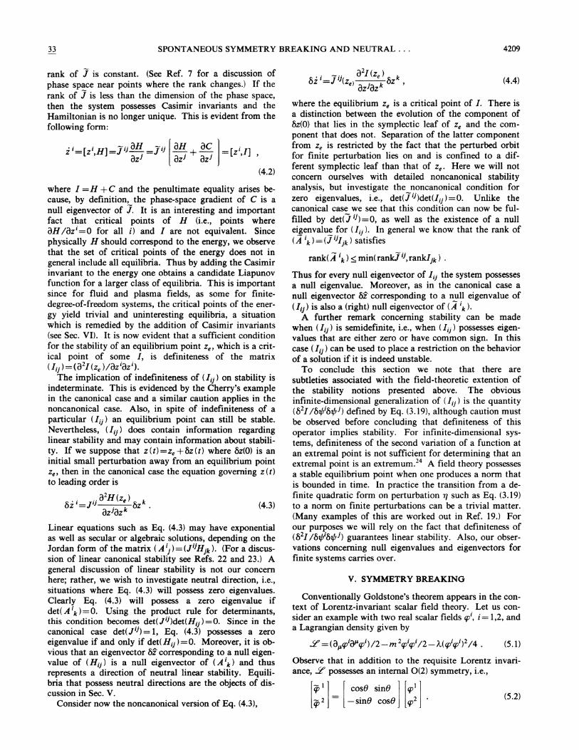
rank of J is constant. (See Ref. 7 for a discussion of phase space near points where the rank changes.) If the rank of J is less than the dimension of the phase space, then the system possesses Casimir invariants and the Hamiltonian is no longer unique. This is evident from the following form:
il=[ZiH]=Jij3~=Jij[3~+ 3C: ]=[Zi I ] , 3zJ 3zJ 3zJ "
(4.2)
where I =H +C and the penultimate equality arises because, by definition, the phase-space gradient of C is a null eigenvector of J. It is an interesting and important fact that critical points of H (i.e., points where 3H 13zi=0 for all i) and I are not equivalent. Since physically H should correspond to the energy, we observe that the set of critical points of the energy does not in general include all equilibria. Thus by adding the Casimir invariant to the energy one obtains a candidate Liapunov function for a larger class of eqUilibria. This is important since for fluid and plasma fields, as some for finitedegree-of-freedom systems, the critical points of the energy yield trivial and uninteresting equilibria, a situation which is remedied by the addition of Casimir invariants (see Sec. VI). It is now evident that a sufficient condition for the stability of an equilibrium point Ze' which is a critical point of some I, is definiteness of the matrix (lij )=W2I(ze lI3z i3z i ).
The implication of indefiniteness of (Iij ) on stability is indeterminate. This is evidenced by the Cherry's example in the canonical case and a similar caution applies in the noncanonical case. Also, in spite of indefiniteness of a particular (Iij ) an equilibrium point can still be stable. Nevertheless, (Ii}) does contain information regarding linear stability and may contain information about stability. If we suppose that z(t)=ze+&(t) where &(0) is an initial small perturbation away from an equilibrium point Ze' then in the canonical case the equation governing z (t) to leading order is
.' .. 32H(ze) k 8z '=J'J . & (4.3)
3zJ3zk
Linear equations such as Eq. (4.3) may have exponential as well as secular or algebraic solutions, depending on the Jordan form of the matrix ( A ij ) = (JilHjk ). (For a discussion of linear canonical stability see Refs. 22 and 23.) A general discussion of linear stability is not our concern here; rather, we wish to investigate neutral direction, i.e., situations where Eq. (4.3) will possess zero eigenvalues. Clearly Eq. (4.3) will possess a zero eigenvalue if det( A i k ) = O. Using the product rule for determinants, this condition becom~ det(Jij)det(Hij)=O. Since in the canonical case det(JiJ) = 1, Eq. (4.3) possesses a zero eigenvalue if and only if det( Hi}) =0. Moreover, it is obvious that an eigenvector 8Z corresponding to a null eigenvalue of (Hij ) is a null eigenvector of (A I k) and thus represents a direction of neutral linear stability. Equilibria that possess neutral directions are the objects of discussion in Sec. V.
Consider now the noncanonical version of Eq. (4.3),
. - .. 3 21 (ze ) k 8i'=J'J(ze) } k 8z ,
3z 3z (4.4)
where the equilibrium Ze is a critical point of I. There is a distinction between the evolution of the component of 8z(0) that lies in the symplectic leaf of Ze and the component that does not. Separation of the latter component from Ze is restricted by the fact that the perturbed orbit for finite perturbation lies on and is confined to a different symplectic leaf than that of Ze' Here we will not concern ourselves with detailed noncanonical stability analysis, but investigate the noncanonical condition for zero eigenvalues, i.e., det(] i})det(Iij) =0. Unlike the canonical case we see that this condition can now be fulfilled by dedi ij) = 0, as well as the existence of a null eij~valu~ .~or (lij)' In general we know that the rank of (A 'k)=(J'JIjk ) satisfies
rankcA Ik ):::;; min(ranklij,rankIjk ) •
Thus for every null eigenvector of Iij the system possesses a null eigenvalue. Moreover, as in the canonical case a null eigenvector 8Z corresponding to a null eigenvalue of ( Ii) ) is also a (right) null eigenvector of (A i k ).
A further remark concerning stability can be made when (Ii}) is semidefinite, i.e., when (Iij ) possesses eigenvalues that are either zero or have common sign. In this case (Ii}) can be used to place a restriction on the behavior of a solution if it is indeed unstable.
To conclude this section we note that there are subtleties associated with the field-theoretic extention of the stability notions presented above. The obvious infinite-~im~nsional generalization of (Ii}) is the quantity (82I18t/18t/JJ) defined by Eq. (3.19), although caution must be observed before concluding that definiteness of this operator implies stability. For infinite-dimensional systems, definiteness of the second variation of a function at an extremal point is not sufficient for determining that an extremal point is an extremum.24 A field theory possesses a stable equilibrium point when one produces a norm that is bounded in time. In practice the transition from a definite quadratic form on perturbation 11 such as Eq. (3.19) to a norm on finite perturbations can be a trivial matter. (Many examples of this are worked out in Ref. 19.) For our purposes we will rely on the fact that definiteness of (821 18~8t/Jj) guarantees linear stability. Also, our observations concerning null eigenvalues and eigenvectors for finite systems carries over.
V. SYMMETRY BREAKING
Conventionally Goldstone's theorem appears in the context of Lorentz-invariant scalar field theory. Let us consider an example with two real scalar fields qi, i= 1,2, and a Lagrangian density given by
2'=(3p.qidl'qi)/2-m 2qlqlI2-'A(qiq:l)2/4. (5.1)
Observe that in addition to the requisite Lorentz invariance, 2' possesses an internal 0(2) symmetry, i.e.,
[q, I ] = [ co~B sinB ] [epl]. q, 2 - smB cosB ep2 (5.2)
4210 P. J. MORRISON AND S. ELIEZER 33
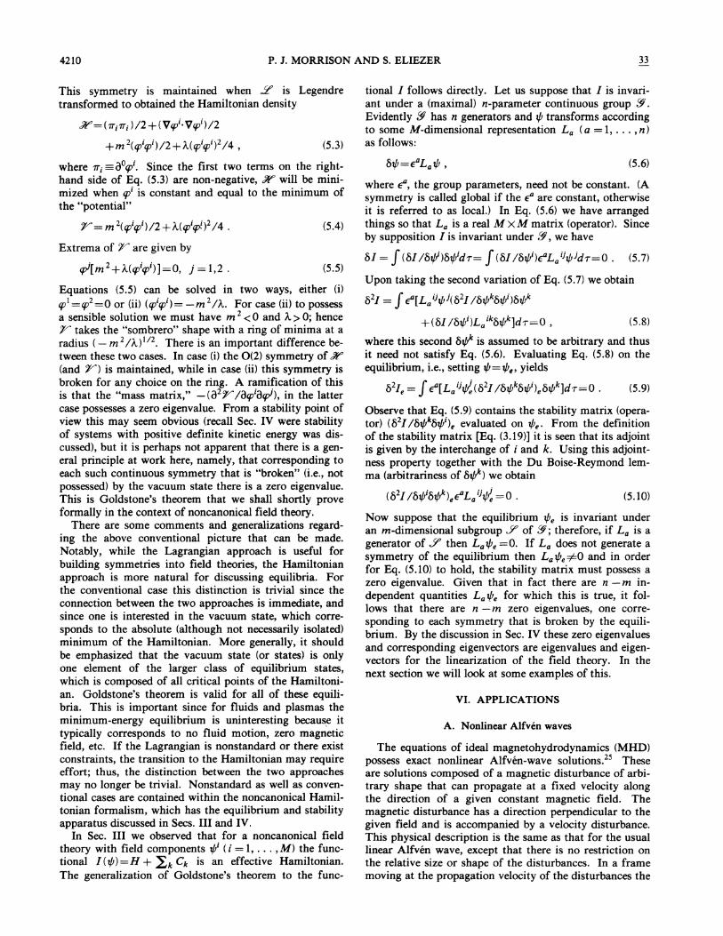
This symmetry is maintained when .!t' is Legendre transformed to obtained the Hamiltonian density
K=(1T(Trj )/2 + (Vlf.i·Vlf.i)/2
(5.3)
where 1Tj == aOq/. Since the first two terms on the righthand side of Eq. (5.3) are non-negative, K will be minimized when qJi is constant and equal to the minimum of the "potential"
r=m2(qJiqJi)/2+'A.(q/q>!)2/4.
Extrema of r are given by
q:J[m2+'A.(qJiqJi)] =0, j = 1,2.
(5.4)
(5.5)
Equations (5.5) can be solved in two ways, either (i) qJl =qJ2=0 or (ii) (qJiqJl)= _m 2 I'A.. For case (ii) to possess a sensible solution we must have m 2 < 0 and 'A. > 0; hence r takes the "sombrero" shape with a ring of minima at a radius (- m 2/'A.)1/2. There is an important difference between these two cases. In case (i) the 0(2) symmetry of K (and r) is maintained, while in case (ii) this symmetry is broken for any choice on the ring. A ramification of this is that the "mass matrix," _(a2r laqJiaq:J), in the latter case possesses a zero eigenvalue. From a stability point of view this may seem obvious (recall Sec. IV were stability of systems with positive definite kinetic energy was discussed), but it is perhaps not apparent that there is a general principle at work here, namely, that corresponding to each such continuous symmetry that is "broken" (i.e., not possessed) by the vacuum state there is a zero eigenvalue. This is Goldstone's theorem that we shall shortly prove formally in the context of noncanonical field theory.
There are some comments and generalizations regarding the above conventional picture that can be made. Notably, while the Lagrangian approach is useful for building symmetries into field theories, the Hamiltonian approach is more natural for discussing equilibria. For the conventional case this distinction is trivial since the connection between the two approaches is immediate, and since one is interested in the vacuum state, which corresponds to the absolute (although not necessarily isolated) minimum of the Hamiltonian. More generally, it should be emphasized that the vacuum state (or states) is only one element of the larger class of equilibrium states, which is composed of all critical points of the Hamiltonian. Goldstone's theorem is valid for all of these equilibria. This is important since for fluids and plasmas the minimum-energy equilibrium is uninteresting becaus~ it typically corresponds to no fluid motion, zero magnetic field, etc. If the Lagrangian is nonstandard or there exist constraints, the transition to the Hamiltonian may require effort; thus, the distinction between the two approaches may no longer be trivial. Nonstandard as well as conventional cases are contained within the noncanonical Hamiltonian formalism, which has the equilibrium and stability apparatus discussed in Secs. III and IV.
In Sec. III we observed that for a noncanonical field theory with field components t/Ji (i = I, ... ,M) the functional I(t/J)=H + ~k Ck is an effective Hamiltonian. The generalization of Goldstone's theorem to the func-
tional I follows directly. Let us suppose that I is invariant under a (maximal) n-parameter continuous group [§. Evidently [§ has n generators and t/J transforms according to some M-dimensional representation La (a = 1, ... ,n) as follows:
(5.6)
where~, the group parameters, need not be constant. (A symmetry is called global if the ~ are constant, otherwise it is referred to as local.) In Eq. (5.6) we have arranged things so that La is a real MXM matrix (operator). Since by supposition] is invariant under [§, we have
M = f (&1 If)ftJ)8t/idT= f (&1 18t/Ji)~L/jt/JjdT=0. (5.7)
Upon taking the second variation of Eq. (5.7) we obtain
82] = f ~[L/jt/Jj(821 18t/Jk8t/i)8~ (5.8)
where this second 8~ is assumed to be arbitrary and thus it need not satisfy Eq. (5.6). Evaluating Eq. (5.8) on the equilibrium, i.e., setting t/J=t/Je, yields
821e = f ~[La iitft!(82] 18~8t/i)e8t/Jk]dT=0 . (5.9)
Observe that Eq. (5.9) contains the stability matrix (operator) (821ISt/JkSt/i)e evaluated on t/Je. From the definition of the stability matrix [Eq. (3.19)] it is seen that its adjoint is given by the interchange of i and k. Using this adjointness property together with the Du Boise-Reymond lemma (arbitrariness of St/Jk) we obtain
(82I/8t/iS~)e~L/itft! =0. (5.10)
Now suppose that the equilibrium t/Je is invariant under an m-dimensional subgroup .Y of [§; therefore, if La is a generator of.Y then Lat/Je=O. If La does not generate a symmetry of the equilibrium then Lat/Je=l=O and in order for Eq. (5.10) to hold, the stability matrix must possess a zero eigenvalue. Given that in fact there are n - m independent quantities La "'e for which this is true, it follows that there are n - m zero eigenvalues, one corresponding to each symmetry that is broken by the equilibrium. By the discussion in Sec. IV these zero eigenvalues and corresponding eigenvectors are eigenvalues and eigenvectors for the linearization of the field theory. In the next section we will look at some examples of this.
VI. APPLICATIONS
A. Nonlinear AIfven waves
The equations of ideal magnetohydrodynamics (MHD) possess exact nonlinear Alfven-wave solutions.25 These are solutions composed of a magnetic disturbance of arbitrary shape that can propagate at a fixed velocity along the direction of a given constant magnetic field. The magnetic disturbance has a direction perpendicular to the given field and is accompanied by a velocity disturbance. This physical description is the same as that for the usual linear Alfveo wave, except that there is no restriction on the relative size or shape of the disturbances. In a frame moving at the propagation velocity of the disturbances the
33 SPONTANEOUS SYMMETRY BREAKING AND NEUTRAL ... 4211
nonlinear Alfven wave can be viewed as a stationary equilibrium state. We will see that this equilibrium does not possess a symmetry of its effective Hamiltonian; hence, there exists a zero eigenvalue.
For simplicity we discuss symmetry breaking by the nonlinear Alfven wave in the context of reduced magnetohydrodynamics (RMHD). This system was derived26•27
in the context of controlled fusion for modeling some dominant physics of the tokamak machine, but more generally it may be applicable whenever there is a strong magnetic field and one desires to describe perpendicular motion. Previously, the presence of the nonlinear Alfven wave in this model was discussed in Ref. 28. Here we use RMHD since it can describe the nonlinear Alfven wave with only two scalar fields, although we emphasize that the results we present hold true for the ideal MHD "parent" of the RMHD model.
The small parameter on which the RMHD reduction is based is the so-called inverse aspect ratio E=a IRa, where Ro is a characteristic length in the direction of the dominant magnetic field and a is a characteristic length of the direction perpendicular to this. For a tokmak Ro is the major radius of the torus, while a is the minor radius. The magnetic and velocity fields take the following divergenceless (to the order indicated) forms:
(6.1)
where t/I is a "stream function" for the magnetic field, which is proportional to the flux through a poloidal cut of the torus (it is also the parallel component of the vector potential), and qJ is the usual velocity stream function. Both t/I and qJ are functions z and of the plane coordinates perpendicular to 'Z. The field variables of RMHD are t/I and the scalar vorticity U =z·Vxv. Evidently, U is related to the stream function through U = VtqJ, while similarly the current in the 'Z direction (- J) is related to t/I through J = Vtt/l. The equations29 governing the RMHD fields can be compactly written in terms of normalized variables as follows:
Ut=[U,qJ]+[t/I,J)-Jz ,
t/lt = [t/I,qJ]-qJz ,
(6.2)
(6.3)
where the square bracket [, ] in polar coordinates is defined by
(6.4)
Observe that if one sets t/I=O then Eqs. (6.2) and (6.3) reduce to the well-known two-dimensional Euler equations of fluid mechanics.
Equations (6.2)-(6.4) posses a Hamiltonian description in terms of the following noncanonical Poisson bracket:30 - 34
IF,Gj = J I U[Fu,Gu ] +t/I([F""Gu ] + [G""Fu ])
(6.5)
where F u is a shorthand for the functional derivative3S
BF IBU and az means a/az. The conserved energy for this system is
H =+ J ( 1 V1qJ 12+ 1 V1t/lI2)dT. (6.6)
Using Eqs. (6.5) and (6.6), Eqs. (6.2) and (6.3) can be written in the following concise form:
t/lt=lt/I,Hj,
Ut=IU,Hj. (6.7)
The bracket of Eq. (6.5) has the following Casimir invariants:
C=J.Jt/ldT,
C=AJ t/lUdT, (6.8)
which corresJ>ond respectively to magnetic and cross helicities. Here A and A are constants.
We now can construct variational principles for equilibria, and thus investigate stability by means of the stability matrix. In fact, this calculation was previously done in Ref. 20, where it was observed for the nonlinear Alfven wave that the stability matrix did not quite provide a norm for stability. Technically the stability matrix provides a prenorm, i.e., a "norm" with degeneracy. We are now in a position to explain this degeneracy, since in general degeneracies correspond to zero eigenvalues of the stability matrix, which in turn arise from broken symmetries. The effective Hamiltonian36 for the Alfven wave is
1=+ J( IV1qJ1 2+ IV1t/lI2_2AV1qJ·V1t/l)dT. (6.9)
Variation of I yields the following eqUilibrium equations:
BIIBU=-qJ+At/I=O, (6.10)
BI IBt/I= -J +AU =0 .
These equations become effectively redundant if A= ± 1 and their solution is qJ= ±t/I, where the spatial dependence is unrestricted. Thus the shape of the magnetic disturbance is arbitrary and it is paralleled by the velocity flow corresponding to qJ. Let us consider the case where A= -1 and rewrite Eq. (6.9) as follows:
1=+ J I V1(qJ+t/I) 1 2dT . (6.11)
Evidently Eq. (6.11) is invariant under the transformation
[~]= [a ±1-d] [qJ] t/I ±1-a d t/I'
(6.12)
where a and d are arbitrary except a +d=l= 1. This group is really a single-parameter local continuous group with two Z2 subgroups. The upper sign corresponds to the subgroup connected to the identity; it has the following elements:
(6.13)
where a is arbitrary. The generator corresponding to the second (continuous) element of (6.13) is
L=[~1 ~l· (6.14)
This symmetry is broken by any choice for the Alfven
4212 P. J. MORRISON AND S. ELIEZER 33
wave equilibrium. Let us now show this directly. Suppose that .,pe is a
choice for a spatially dependent equilibrium magnetic perturbation with corresponding velocity perturbation rpe = -.,pe· The equilibrium state is then given by the following column vector:
~e=[~~el· (6.15)
The upper entry corresponds to the equilibrium-velocity stream function. According to the analysis of Sec. V, the quantity (L ij~~) should be a null eigenvector of the stability matrix. The stability matrix ([ij) in this case is given by
(6.16)
From Eq. (6.16) it is clear that JijELjk~:=O for i= 1,2. (Here we have defined the stability matrix in terms of the variable rp instead of the dynamical variable U; in particular, J \1 =f:J2J 1f:Jrp2.) It is now evident why the analysis of Ref. 20 resulted in a prenorm: the Alfven wave breaks symmetry.
B. Solitons and solitary waves
Sometimes nonlinear field theories possess soliton or, more commonly, solitary-wave solutions. These are nonlinear solutions that propagate at constant velocity (c),
with an unchanged shape that may be pulselike or steplike. In the "wave frame", which moves at velocity c, the shape corresponds to an equilibrium state. Loosely speaking, solitons are solitary waves with the further property that when two collide the original shapes and velocities are preserved after the interaction. Typically this is only approximately true for solitary waves. Solitons have all or part of the inverse-scattering machinery available for integration (see, e.g., Ref. 37). The distinction between solitons and solitary waves will not concern us here; our results are not restricted to the relatively rare case of soliton solutions. In fact our results apply for equilibria of any field theory with a conserved momentum.
Field theories that have soliton or solitary-wave solutions can be either canonical or noncanonical. For example, the rp4 Klein-Gordon equation, the sine-Gordon equation, and the cubic nonlinear SchrOedinger equation are canonical (see, e.g., Refs. 37 and 38), while the Korteweg-de Vries (KdV) equation and the regularizedlong-wave equation are naturally non~anonical (see, e.g., Refs. 37 and 39 for the former and Ref. 40 for the latter). As an example we will work out the case for a single KdV soliton. Stability for this example has previously been investigated.41 ,42
Consider the KdV equation transformed into a frame moving at a constant velocity c,
(6.17)
This equation possesses the following Poisson bracket due to Gardner:39
I co a ( F, G J = _ co (f:JF If:Ju) ax (f:JG If:Ju)dx . (6.18)
The Hamiltonian and Casimir invariant are given, respectively, by
H= I_COco (u 3/6-u;/2-cu 2/2)dx, (6.19)
C=AI_ooooudx.
For our purposes the Casimir C is not needed. The "momentum" I u 2dx has been added to the Hamiltonian in order to boost the system into the wave frame. Thus we have J =H and
(6.20)
Equilibrium requires that UJOC - cu + U 212 = 0, which has the desired solution Ue = A sech2( kx), where A = ± VUk and k 2=c/4. The specification of c at the outset determines a particular equilibrium solution. Observe that J is invariant under space translation. This is evident from Eq. (6.20) since if f:Ju =EUx , we obtain f:JJ=O upon enforcing the boundary conditions U (± 00 )=0. The choice of U = Ue for an equilibrium breaks this symmetry; thus, we expect a zero eigenvalue. Consider the second variation
f:J2J = r:co f:Ju (u -c +a2/ax2)f:J'17dx . (6.21)
The stability operator u -c +a2/ax 2 possesses the null eigenvalue when evaluated at U =Ue • The corresponding eigenfunction is given by
f:J'17=EUx =E'sech2(kx)tanh(kx) , (6.22)
as can be shown directly. Here E and E' are constants.
VII. CONCLUSIONS
In Secs. II and III we have reviewed the noncanonical Hamiltonian formalism for finite-degree-of-freedom systems and field theories, respectively. This formalism is based upon a generalization of the Poisson bracket. Unlike typical quantum fields, Poisson brackets for continuous media fields that are written in terms of Eulerian variables, have explicit linear dependence upon the field components. Additionally, because of degeneracies there are Casimir invariants. Casimir invariants are important because they enlarge the class of equilibria obtainable from variational principles. Typically for media fields, variation of the energy alone yields uninteresting equilibria, a situation that is remedied by using the Casimir constraints. The so-called "thermodynamic" variational principles of plasma physics43 are Casimir-constrained variational principles. The noncanonical formalism explains the existence of these Casimir invariants, explains the connection between the equilibrium-variational principles and the dynamics [see, e.g., Eqs. (3.17) and (4.2)], and provides a framework for finding new Casimir invariants.
Stability was treated in Sec. IV. For canonical finitedegree-of-freedom-systems the Hamiltonian can serve as a Liapunov function for determining nonlinear stability. If the Hamilton has standard kinetic energy and potential energy terms, then the sign of the curvature at the equilibrium point provides a necessary and sufficient condition
33 SPONTANEOUS SYMMETRY BREAKING AND NEUTRAL ... 4213
for nonlinear stability. If the Hamiltonian is not of this standard form then one must examine the curvature of the entire Hamiltonian. A sufficient condition for stability is definiteness of the stability matrix (Hij ). In the noncanonical case the situation is complicated. If one can find an I for which the desired equilibrium is an extremal point and for which (Iij ) is definite, then a sufficient condition for nonlinear stability is obtained. We have shown that if (Iij) is indefinite by possessing zero eigenvalues, then the zero eigenvalues and eigenvectors of (Iij ) imply neutral stability for the linearized system. The zero eigenvectors of (Iij ) are neutral directions. Neutral linear stability for infinite-dimensional systems similarly arises if (f/Ilot/it"J) has zero directions.
In Sec. V Goldstone's theorem was adapted to the noncanonical formalism. It was emphasized that the Hamiltonian formalism is the natural place to discuss symmetry breaking since the Hamiltonian or its generalization I provides a variational principle for equilibria. If an equilibrium obtained in this way has less symmetry than that of I, then for each such broken continuous symmetry there is a zero eigenvalue of (Iij)' The corresponding null eigendirection of (IiJ ) is a null eigendirection of the linear equations.
There are two features of our presentation of Goldstone's theorem in the noncanonical context that differ from the "conventional" context discussed at the beginning of Sec. V. Firstly, the conventional case makes a distinction between coordinates and momenta, the neutral direction being solely in the configurations pace. Our presentation includes this possibility, but is not restricted to it. Secondly, in the noncanonical context we have made the connection between symmetry and neutral directions of the linearized system, but in the conventional case it is apparent that the neutral direction persists nonlinearly. Neutral stability on the linear level is necessary but not sufficient for the nonlinear level.
·Permanent address: Soreq Nuclear Research Centre, 70600 Yarne, Israel.
IFor a standard review of gauge theories see E. S. Albers and B. W. Lee, Phys. Rep. 9C, 1 (1973).
2J. Goldstone, Nuovo Cimento 19, 154 (1961). 3y. Nambu and G. Jona-Lasinio, Phys. Rev. 122, 345 (1961). 4J. Goldstone, A. Salam, and S. Weinberg, Phys. Rev. 127, 965
(1962). 5See, for example, D. Forster, in Frontiers in Physics, edited by
D. Pines (Benjamin-Cummings, Reading, Mass. 1975). 6E. C. G. Sudarshan and N. Mukunda, Classical Mechanics--a
Modern Perspective, 2nd ed. (Krieger, Melbourne, 1983). 7 A. Weinstein, J. Diff. Geom. 18,523 (1983). 8R. J. Littlejohn, Mathematical Methods in Hydrodynamics and
Integrability in Dynamical Systems, edited by M. Tabor and Y. M. Treve (AlP, New York, 1982).
9p. J. Morrison, in Mathematical Methods in Hydrodynamics and Integrability in Dynamical Systems, edited by M. Tabor and Y. M. Treve (AlP, New York, 1982).
IOJ. E. Marsden and P. J. Morrison, Contemp. Math. 28, 133 (984).
Sometimes it can be shown that, although a linear neutral direction exists, the system is nonlinearly stable. In the noncanonical formalism an approach arises because the quantity I is not unique. The lack of uniqueness is due to freedom in the choice of the Casimir constraint, Le., in the definition I =H + C one can replace C by a function of C, but still produce the same dynamics and obtain the same equilibrium upon variation. The quantity (jij), though, will in general be different. In particular if 1= H + A.F (C) where A is a constant chosen so that I and I yield the same equi.librium, then (iij ) - (Iij )
=(FccIFc)(aC/az')(aC/az'). (Here the SUbscript C means derivative with respect to C.) This additional term can, but need not, result in definiteness of (ii}) and thus stability.44,45 If one attempts this for the nonlinear Alfven wave discussed in Sec. VII it is seen that neutral stability persists.
Finally, we speculate about some ways that neutral stability can be removed. In the conventional case this is achieved by the Higgs46 mechanism when the scalar fields are coupled to the electromagnetic gauge field. The addition of new physics into a continuous-media model can achieve the same end. This could be done either by the introduction of dissipation or by coupling to new fields.
ACKNOWLEDGMENTS
This work was supported by U.S. Department of Energy Contract No. DE-FG05-S0ET-530SS. We would like to thank R. D. Hazeltine, J. D. Meiss, and D. pfirsch for critically reading a preliminary version of this paper. One of us (S.E.) would like to acknowledge a useful conversation with Y. Ne'eman. The other of us (P.J.M.) is indebted to D. D. Holm, T. Ratiu, A. Weinstein, and especially to J. E. Marsden for many fruitful discussions pertaining to stability; also, useful conversations with C. Litwin and R. S. MacKay are thankfully acknowledged.
IIp. A. M. Dirac, Can. J. Math. 2, 129 (1950); Lectures on Quantum Mechanics (Yeshiva University, New York, 1964).
12A. Hanson, T. Regge, and C. Teitelboim, Constrained Hamiltonian Systems (Accademici Nazionale dei Lincei, Rome, 1976).
13K. Sundermeyer, Constrained Dynamics, Yol. 169 of Lecture Notes in Physics (Springer-Yerlag, Berlin, 1982),
14y. I. Arnold, Ann. Inst. Fourier 16, 319 (1966). 15J. E. Marsden and A. Weinstein, Rep. Math. Phys. 5, 121
(974). 16p. J. Morrison and R. D. Hazeltine, Phys. Fluids 27, 886
(1984). 171. E. Marsden, P. J. Morrison, and A. Weinstein, Contemp.
Math. 28, 115 (1984). 18y. I. Arnold, Am. Math. Soc. Transl. 79, 267 (1969). 19D. D. Holm, J. E. Marsden, T. Ratiu, and A. Weinstein, Phys.
Rep. 123, 1 (1985). 2oR. D. Hazeltine, D. D. Holm, and P. J. Morrison, in Proceed
ings of the International Conference on Plasma Physics, edited by M. Q. Tran and M. L. Saw ley (Ecole Poly technique, Lausanne, Switzerland, 1984), Yol. 2, p. 204. The results of
4214 P. J. MORRISON AND S. ELIEZER 33
this paper are reproduced in Ref. 19. 21T. M. Cherry, Trans. Cambridge Philos. Soc. 23, 199 (1925);
See E. T. Whittaker, Analytical Dynamics (Cambridge, London, 1937), Sec. 182, p. 142; and A. Wintner, The Analytical Foundations of Celestial Mechanics (Princeton University, Princeton, 1947), Sec. 136, p. 101.
22J. Moser, Commun. Pure Appl. Math. 11,81 (1958). 23R. S. MacKay, in Nonlinear Phenomena and Chaos, edited by
S. Sarker (Hilger, Bristol, 1986), p. 254. 241. M. Gelfand and S. Y. Fomin, Calculus of Variations
(Prentice-Hall, Englewood Cliffs, 1963). 25C. Walen, Ark. Mat. Astronom. Fys. 3OA, no. 15 (1944); 31B,
no. 3 (1944). See H. Alfven, Cosmic Electrodynamics (Clarenden, Oxford, 1950), p. 86.
26M. N. Rosenbluth, D. A. Monticello, H. R. Strauss, and R. B. White, Phys. Fluids 19. 198 (1976).
27H. R. Strauss, Phys. Fluids 19, 134 (1976). 28p. J. Morrison and R. D. Hazeltine, Proceedings of the Sher
wood Theory Meeting, Arlington, Yirginia, 1983 (unpublished).
29This system of equations is known as 10w-(3 RMHD because pressure is neglected. A version that includes pressure is given in H. R. Strauss, Phys. Fluids 20, 1354 (1977).
30p. J. Morrison and R. D. Hazeltine, Phys. Fluids 27, 886 (1984). See also Ref. 10. The first term of this bracket is the noncanonical Poisson bracket for Euler's equations in two dimensions. It appeared in Refs. 9 and 31. The effective Lagrange bracket for this system was introduced by Arnold (see, e.g., Ref. 32). Poisson brackets for three-dimensional vortex flows appeared in Refs. 33 and 34.
31p. J. Morrison, Princeton University Plasma Physics Laboratory Report No. PPPL-1788, 1981 (unpublished); P. J. Olver, J. Math. Anal. Appl. 89,233 (1982).
32y. I. Arnold, Mathematical Methods of Classical Mechanics
(Springer-Yerlag, New York, 1978), Appendix 2. 33p. J. Morrison and J. M. Greene, Phys. Rev. Lett. 45, 790
(1980); 48,569 (1982). 34E. Z. Kuznetzov and A. Y. Mikhailov, Phys. Lett. 77A, 37
(1980). 35For a discussion of boundary conditions and the neglect of
surface terms involved in the definition of this functional derivative see D. Lewis, J. E. Marsden, R. Montgomery, and T. Ratiu, Physica D (to be published), where the Hamiltonian structure for the free-boundary Euler equations is presented.
36If motion is restricted to two dimensions, then more general Alfven-wave solutions are obtainable from variation of the effective Hamiltonian. This is because the integrand of the Casimir invariant C generalizes to UG (t/J), where G is an arbitrary function of t/J. Results similar to those we present here apply for these two-dimensional equilibria.
37M. J. Ablowitz and H. Segur, Solitons and the Inverse Scatter-ing Transform (SIAM, Philadelphia, 1981).
38R. Rajaraman, Phys. Rep. 21, 227 (1975). 39C. S. Gardner, J. Math. Phys. 12, 1548 (1971). 4Op. J. Morrison, J. D. Meiss, and J. R. Cary, Physica lID, 324
(1984). 41A. Jeffrey and T. Kakutani, Indiana Univ. Math. J. 20, 463
(1970). 42T. B. Benjamin, Proc. R. Soc. London Ser. A 328, 153 (1972). 43N. A. Krall and A. W. Trivelpiece, Principles of Plasma Phys
ics (McGraw-Hill, New York, 1973), and references therein; M. D. Kruskal and C. R. Oberman, Phys. Fluids 1, 275 (1958); C. S. Gardner, ibid. 6,839 (1963).
44An example of this is given for the rigid body in Refs. 19 and 45.
45p. J. Morrison, Physica 180,410 (1986). 46p. W. Higgs, Phys. Rev. Lett. 12, 132 (1964).