Split-split Plot Arrangement

The split-split plot arrangement is especially suited for three or more factor experiments where different levels of precision are required for the factors evaluated. This arrangement is characterized by: 1. Three plot sizes corresponding to the three factors; namely, the largest plot for the main

factor, the intermediate size plot for the subplot factor, and the smallest plot for the sub-subplot factor.

2. There are three levels of precision with the main plot factor receiving the lowest

precision, and the sub-subplot factor receiving the highest precision. Example Split-split plot arrangement randomized as an RCBD. Three levels of the whole plot factor, A, two levels of the subplot factor, B, and three levels of the sub-subplot factor, C. Diagram shows the first replicate.

a1b0 subplots a2b1c0

a2b1c2

a2b1c1

a0 Whole plot

a1b1 subplots

a2b0c1

a2b0c0

a2b0c2

Randomization Procedure The randomization procedure for the split-split plot arrangement consists of three parts: 1. Randomly assign whole plot treatments to whole plots based on the experimental design

used. 2. Randomly assign subplot treatments to the subplots. 3. Randomly assign sub-subplot treatments to the sub-subplots. The experimental design used to randomize the whole plots will not affect randomization of the sub and sub-subplots. Expected Mean Squares for the Split-split Plot Arrangement 1

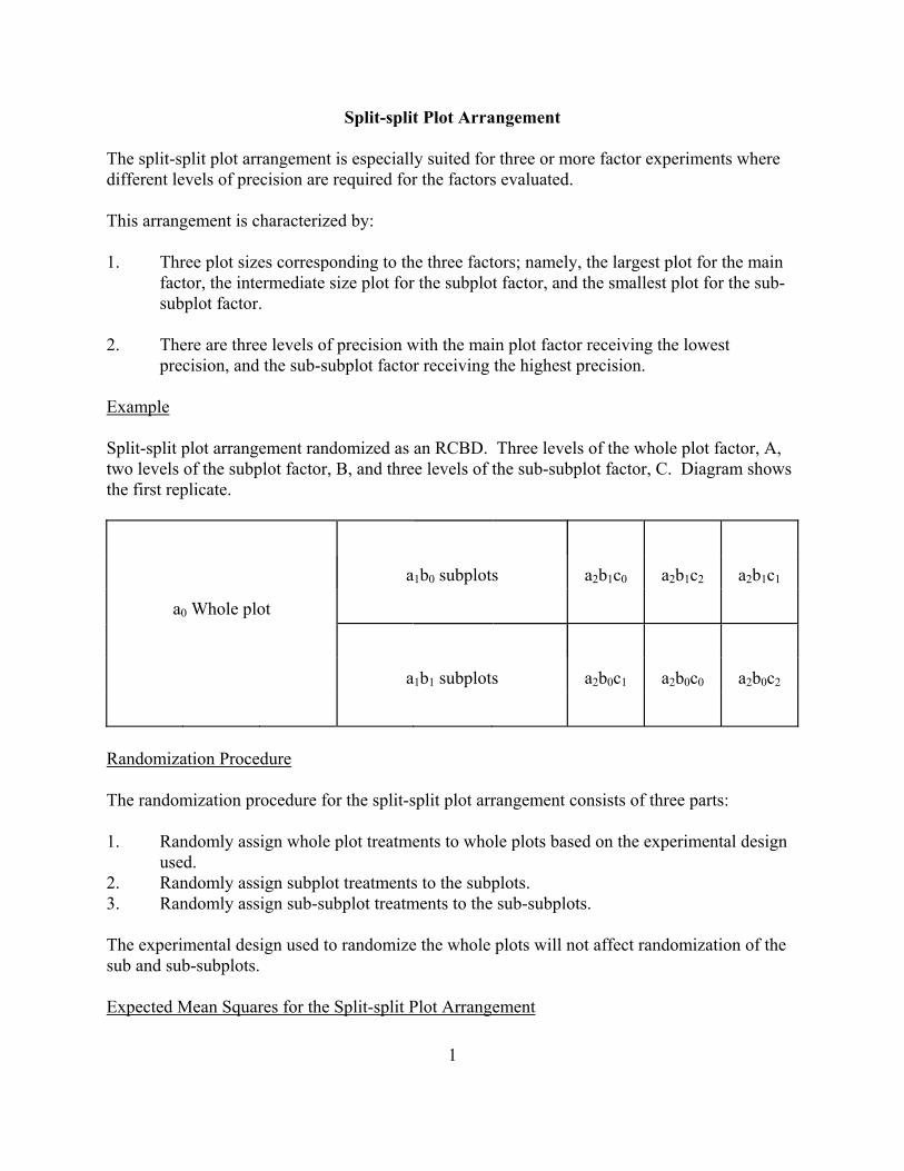
The example to be given will be for an RCBD with factor A as the whole plot factor, factor B as the subplot factor, and factor C as the sup-subplot factor. Factors A, B, and C will be considered random effects. Source of variation

df

Expected mean square

Replicate

r-1

σ2 + cσ2

θ + bcσ2γ + abcrσ2

R A

a-1

σ2 + cσ2

θ + bcσ2γ + rσ2

ABC + rbσ2AC + rcσ2

AB + rbcσ2A

Error (a) = RepxA

(r-1)(a-1)

σ2 + cσ2

θ + bcσ2γ

B

b-1

σ2 + cσ2

θ + rσ2ABC + raσ2

BC + rcσ2AB + racσ2

B AxB

(a-1)(b-1)

σ2 + cσ2

θ + rσ2ABC + rcσ2

AB Error (b) = RepxB(A)

a(r-1)(b-1)

σ2 + cσ2

θ C

c-1

σ2 + rσ2

ABC + raσ2BC + rbσ2

AC + rabσ2C

AxC

(a-1)(c-1)

σ2 + rσ2

ABC + rbσ2AC

BxC

(b-1)(c-1)

σ2 + rσ2

ABC + raσ2BC

AxBxC

(a-1)(b-1)(c-1)

σ2 + rσ2

ABC Error (c) = RepxC(AxB)

ab(r-1)(c-1)

σ2

Total

rabc-1

2

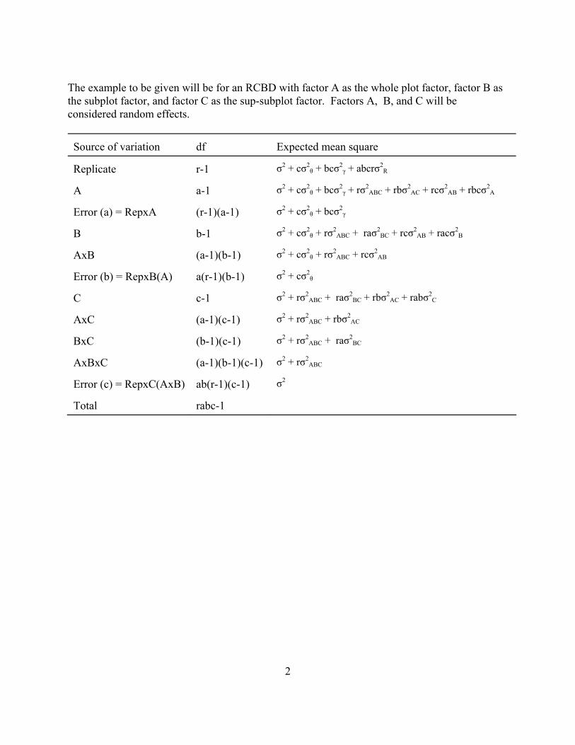
ANOVA of a Split-split Plot Arrangement - Table 1. Data for split-split plot example

Treatments

Replicates

Treatment

Aj

Bk

Cl

1

2

3

4

totals

0

0

0

25.7

25.4

23.8

22.0

96.9

0

0

1

31.8

29.5

28.7

26.4

116.4

0

0

2

34.6

37.2

29.1

23.7

124.6

Subplot tot. Yi00.

92.1

92.1

81.6

72.1

337.9=

Y.00.

0

1

0

27.7

30.3

30.2

33.2

121.4

0

1

1

38.0

40.6

34.6

31.0

144.2

0

1

2

42.1

43.6

44.6

42.7

173.0

Subplot tot. Yi01.

107.8

114.5

109.4

106.9

438.6=

Y.01.

Whole plot tot. Yi0..

199.9

206.6

191.0

179.0

776.5=

Y.0..

1

0

0

28.9

24.7

27.8

23.4

104.8

1

0

1

37.5

31.5

31.0

27.8

127.8

1

0

2

38.4

32.5

31.2

29.8

131.9

Subplot tot. Yi10.

104.8

88.7

90.0

81.0

364.5=

Y.10.

1

1

0

38.0

31.0

29.5

30.7

129.2

1

1

1

36.9

31.9

31.5

35.9

136.2

1

1

2

44.2

41.6

38.9

37.6

162.3

Subplot tot. Yi11.

119.1

104.5

99.9

104.2

427.7=

Y.11.

Whole plot tot. Yi1..

223.9

193.2

189.9

185.2

792.2=

Y.1..

2

0

0

23.4

24.2

21.2

20.9

89.7

2

0

1

25.3

27.7

23.7

24.3

101.0

2

0

2

29.8

29.9

24.3

23.8

107.8

Subplot tot. Yi20.

78.5

81.8

69.2

69.0

298.5=

Y.20.

2

1

0

20.8

23.0

25.2

23.1

92.1

2

1

1

29.0

32.0

26.5

31.2

118.7

2

1

2

36.6

37.8

34.8

40.2

149.4

Subplot tot. Yi21.

86.4

92.8

86.5

94.5

360.2=

Y.21.

Whole plot tot. Yi2..

164.9

174.6

155.7

163.5

658.7=

Y.2..

Rep total Yi...

588.7

574.4

536.6

527.7

2227.4=

Y....

3

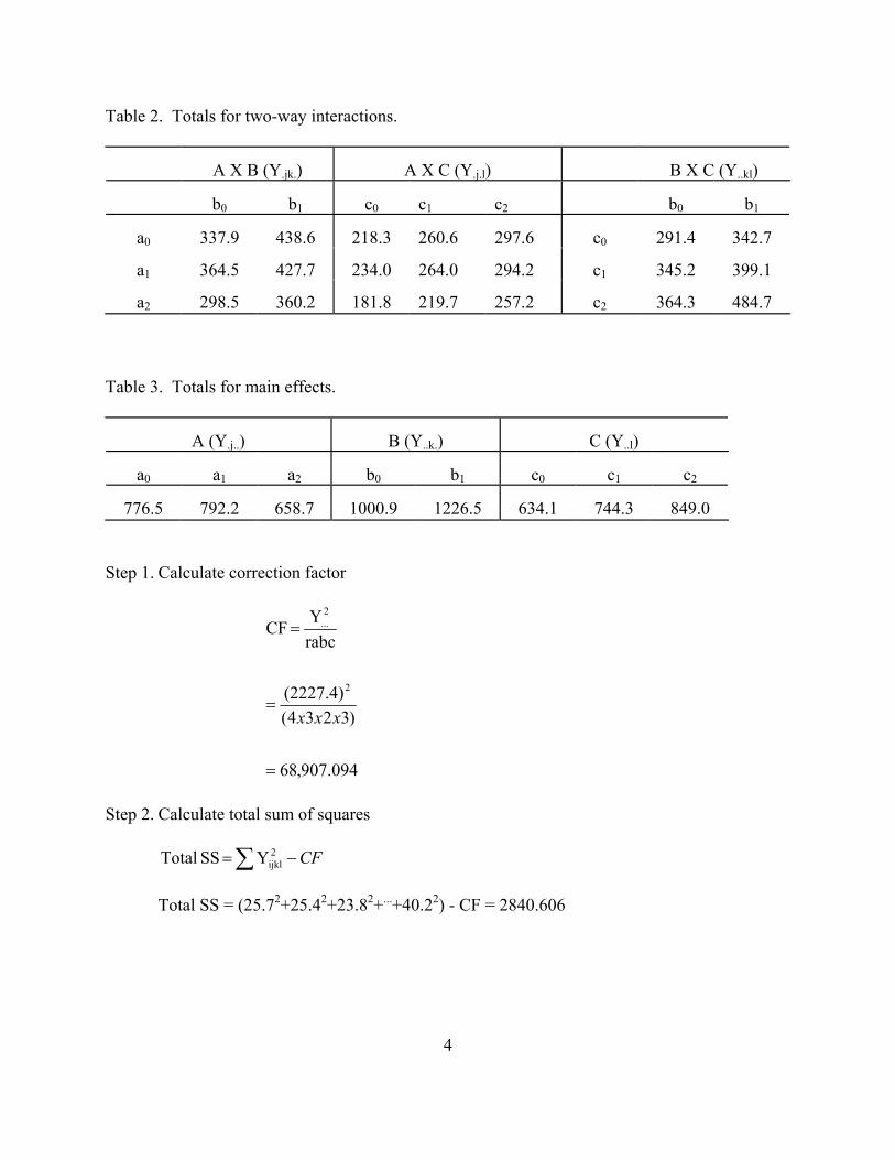
Table 2. Totals for two-way interactions.

A X B (Y.jk.)

A X C (Y.j.l)

B X C (Y..kl)

b0

b1

c0

c1

c2

b0

b1

a0

337.9

438.6

218.3

260.6

297.6

c0

291.4

342.7

a1

364.5

427.7

234.0

264.0

294.2

c1

345.2

399.1

a2

298.5

360.2

181.8

219.7

257.2

c2

364.3

484.7

Table 3. Totals for main effects.

A (Y.j..)

B (Y. k.. )

C (Y..l)

a0

a1

a2

b0

b1

c0

c1

c2

776.5

792.2

658.7

1000.9

1226.5

634.1

744.3

849.0

Step 1. Calculate correction factor

094.907,68

)3234((2227.4)

rabcY CF

2

2...

=

=

=

xxx

Step 2. Calculate total sum of squares

∑ −= CF2ijklY SS Total

Total SS = (25.72+25.42+23.82+...+40.22) - CF = 2840.606

4

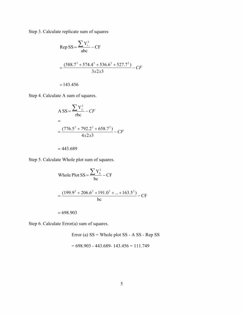
Step 3. Calculate replicate sum of squares

456.143

323)7.5276.5364.574(588.7

CFabc

Y SS Rep

2222

2i...

=

−+++

=

−= ∑

CFxx

Step 4. Calculate A sum of squares.

689.443

324)7.6582.7925.776(

rbcY

SSA

222

2.j..

=

−++

=

−= ∑

CFxx

CF

=

Step 5. Calculate Whole plot sum of squares.

903.698

CFbc

)163.5...191.0206.6(199.9

CFbcY

SSPlot Whole

2222

2ij

=

−++++

−= ∑

=

Step 6. Calculate Error(a) sum of squares.

Error (a) SS = Whole plot SS - A SS - Rep SS

= 698.903 - 443.689- 143.456 = 111.749

5

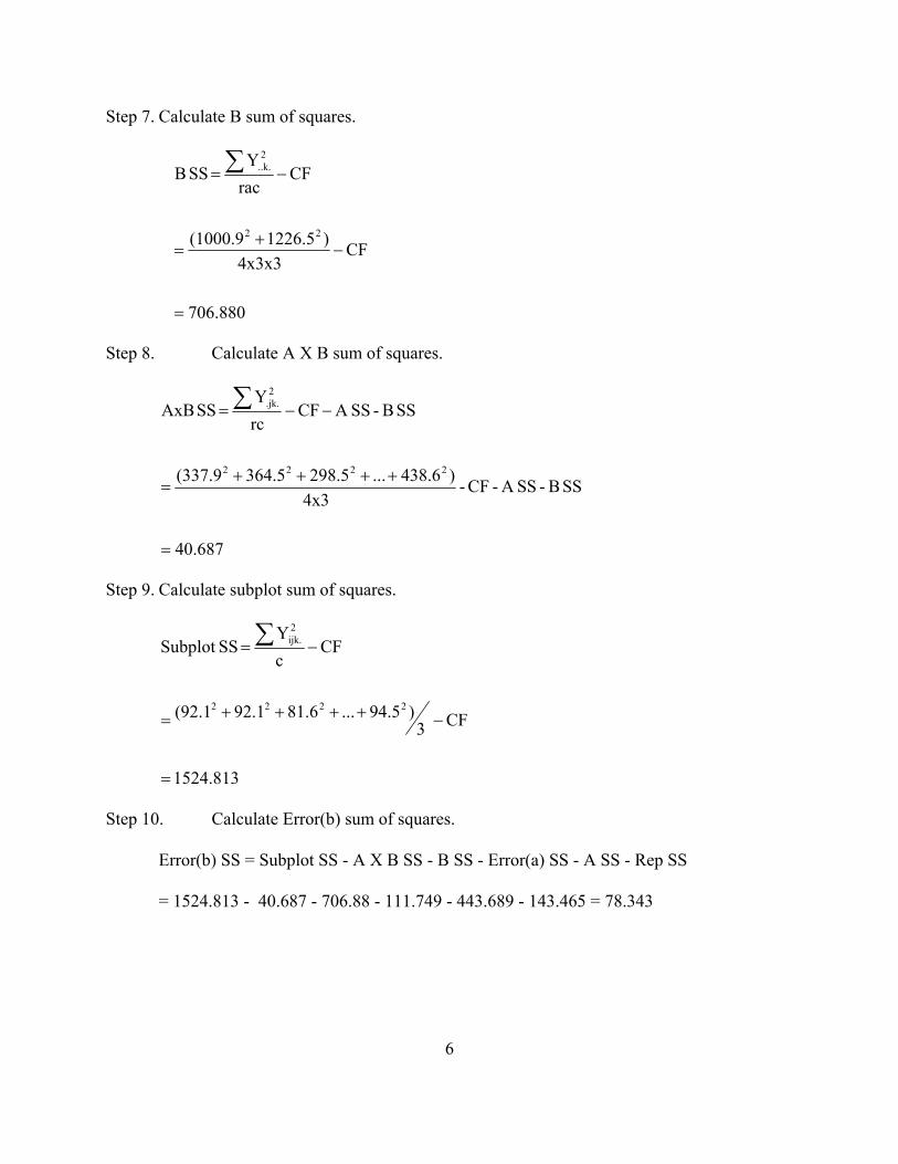
Step 7. Calculate B sum of squares.

706.880

CF4x3x3

)1226.5(1000.9

CFracY

SS B

22

2..k.

=

−+

=

−= ∑

Step 8. Calculate A X B sum of squares.

40.687

SS B - SSA - CF-4x3

)438.6...298.5364.5(337.9

SS B - SSA CFrcY

SS AxB

2222

2.jk.

=

++++=

−−= ∑

Step 9. Calculate subplot sum of squares.

1524.813

CF3)94.5...81.692.1(92.1

CFcY

SSSubplot

2222

2ijk.

=

−++++=

−= ∑

Step 10. Calculate Error(b) sum of squares.

Error(b) SS = Subplot SS - A X B SS - B SS - Error(a) SS - A SS - Rep SS

= 1524.813 - 40.687 - 706.88 - 111.749 - 443.689 - 143.465 = 78.343

6

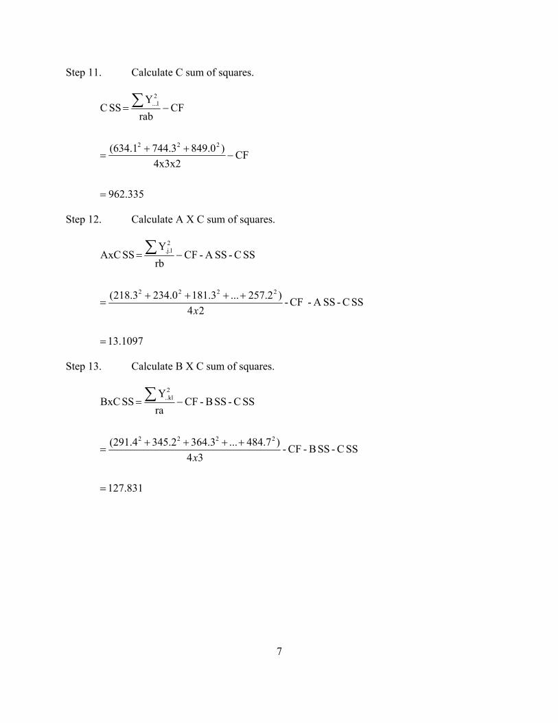
Step 11. Calculate C sum of squares.

962.335

CF4x3x2

)849.0744.3(634.1

CFrab

Y SS C

222

2...l

=

−++

=

−= ∑

Step 12. Calculate A X C sum of squares.

1097.13

SS C - SSA - CF-24

)2.257...3.1810.2343.218(

SS C - SSA - CFrbY

SS AxC

2222

2.j.l

=

++++=

−= ∑

x

Step 13. Calculate B X C sum of squares.

127.831

SS C - SS B - CF -34

)484.7...3.3642.345(291.4

SS C - SS B - CFraY

SS BxC

2222

2..kl

=

++++=

−= ∑

x

7

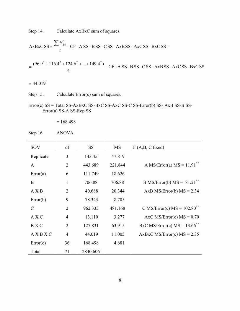
Step 14. Calculate AxBxC sum of squares.

44.019

SS BxC - SS AxC - SS AxB - SS C - SS B - SSA - CF4

)149.4...6.1244.116(96.9

-SS BxC - SS AxC - SS AxB - SS C - SS B - SSA - CF-rY

SS AxBxC

2222

2.jkl

=

−++++

=

= ∑

Step 15. Calculate Error(c) sum of squares. Error(c) SS = Total SS-AxBxC SS-BxC SS-AxC SS-C SS-Error(b) SS- AxB SS-B SS-

Error(a) SS-A SS-Rep SS

= 168.498

Step 16 ANOVA SOV

df

SS

MS

F (A,B, C fixed)

Replicate

3

143.45

47.819

A

2

443.689

221.844

A MS/Error(a) MS = 11.91**

Error(a)

6

111.749

18.626

B

1

706.88

706.88

B MS/Error(b) MS = 81.21**

A X B

2

40.688

20.344

AxB MS/Error(b) MS = 2.34

Error(b)

9

78.343

8.705

C

2

962.335

481.168

C MS/Error(c) MS = 102.80**

A X C

4

13.110

3.277

AxC MS/Error(c) MS = 0.70

B X C

2

127.831

63.915

BxC MS/Error(c) MS = 13.66**

A X B X C

4

44.019

11.005

AxBxC MS/Error(c) MS = 2.35

Error(c)

36

168.498

4.681

Total

71

2840.606

8

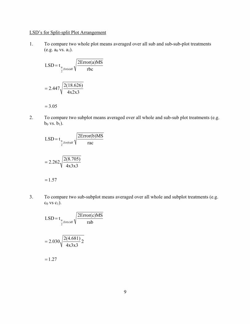
LSD’s for Split-split Plot Arrangement 1. To compare two whole plot means averaged over all sub and sub-sub-plot treatments

(e.g. a0 vs. a1).

3.05

4x2x32(18.626)2.447

rbcS2Error(a)M t LSD

Err(a)df,2α

=

=

=

2. To compare two subplot means averaged over all whole and sub-sub plot treatments (e.g.

b0 vs. b1).

57.1

4x3x32(8.705)2.262

racS2Error(b)M t LSD

Err(b)df,2α

=

=

=

3. To compare two sub-subplot means averaged over all whole and subplot treatments (e.g.

c0 vs c1).

27.1

24x3x3

2(4.681)2.030

rabS2Error(c)M t LSD

Err(c)df,2α

=

=

=

9

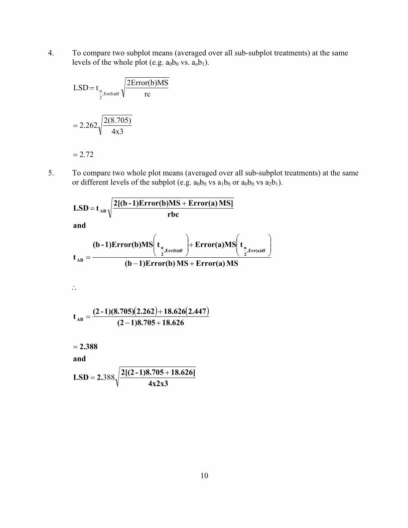
4. To compare two subplot means (averaged over all sub-subplot treatments) at the same levels of the whole plot (e.g. a0b0 vs. aob1).

72.2

4x32(8.705)2.262

rcS2Error(b)M t LSD

Err(b)df,2α

=

=

=

5. To compare two whole plot means (averaged over all sub-subplot treatments) at the same

or different levels of the subplot (e.g. a0b0 vs a1b0 or a0b0 vs a2b1).

( ) ( )

4x2x318.626] 1)8.705-2[(2.2LSD

and2.388

18.6261)8.705(22.44718.6262.2621)(8.705)-(2t

MS Error(a)MS 1)Error(b)(b

tError(a)MStMS1)Error(b)-(bt

andrbc

MS] Error(a) MS1)Error(b)-2[(bt LSD

AB

Err(a)df,2αErr(b)df,

2α

AB

AB

+=

=

+−+

=

∴

+−

+

=

+=

388

10

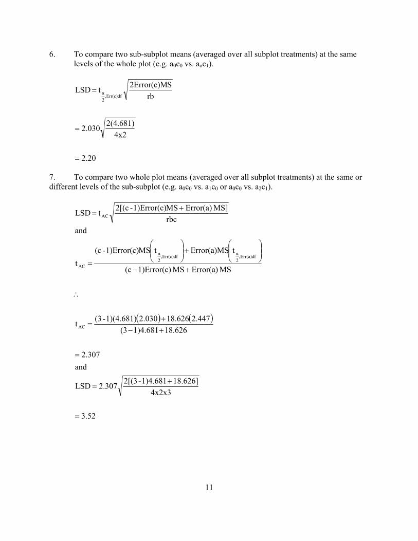
6. To compare two sub-subplot means (averaged over all subplot treatments) at the same levels of the whole plot (e.g. a0c0 vs. aoc1).

2.20

4x22(4.681)2.030

rbS2Error(c)M t LSD

Err(c)df,2α

=

=

=

7. To compare two whole plot means (averaged over all subplot treatments) at the same or different levels of the sub-subplot (e.g. a0c0 vs. a1c0 or a0c0 vs. a2c1).

( ) ( )

52.3

4x2x318.626] 1)4.681-2[(3307.2LSD

and2.307

18.6261)4.681(32.44718.6262.0301)(4.681)-(3t

MS Error(a)MS 1)Error(c)(c

tError(a)MStMS1)Error(c)-(ct

andrbc

MS] Error(a) MS1)Error(c)-2[(c t LSD

AC

Err(a)df,2αErr(c)df,

2α

AC

AC

=

+=

=

+−+

=

∴

+−

+

=

+=

11

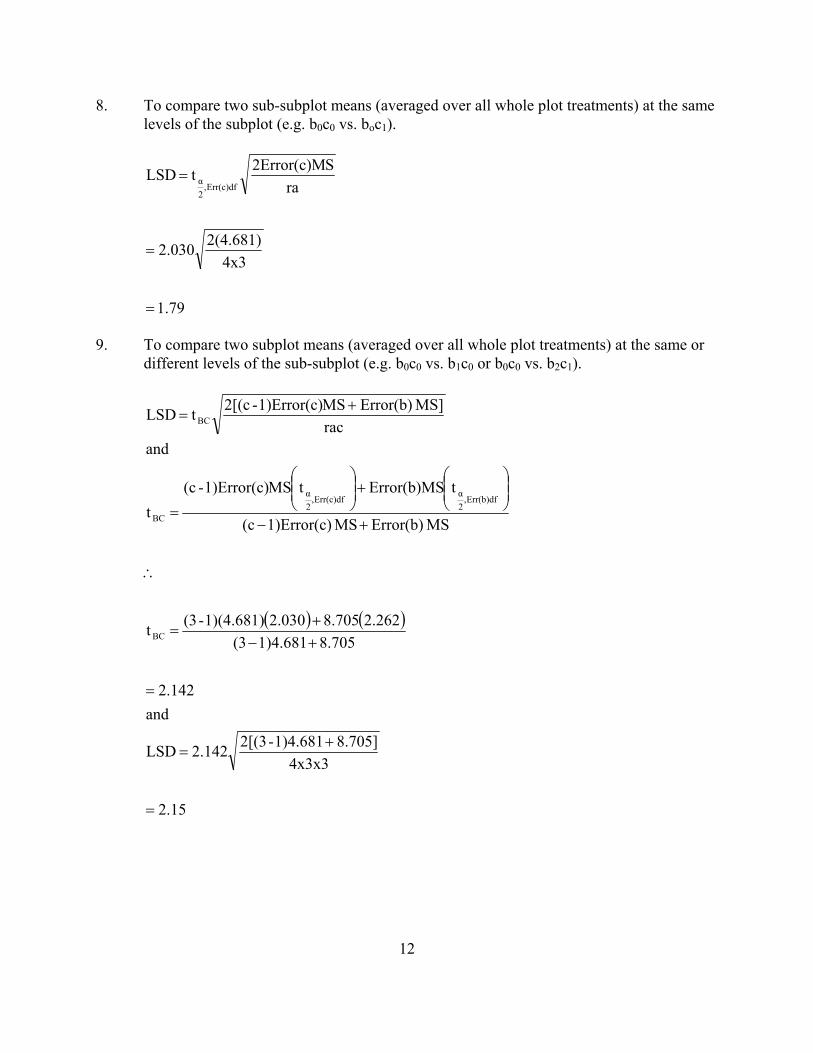
8. To compare two sub-subplot means (averaged over all whole plot treatments) at the same levels of the subplot (e.g. b0c0 vs. boc1).

79.1

4x32(4.681)2.030

raS2Error(c)M t LSD

Err(c)df,2α

=

=

=

9. To compare two subplot means (averaged over all whole plot treatments) at the same or

different levels of the sub-subplot (e.g. b0c0 vs. b1c0 or b0c0 vs. b2c1).

( ) ( )

15.2

4x3x38.705] 1)4.681-2[(3142.2LSD

and2.142

705.81)4.681(32.262705.82.0301)(4.681)-(3t

MS Error(b)MS 1)Error(c)(c

tError(b)MStMS1)Error(c)-(ct

andrac

MS] Error(b) MS1)Error(c)-2[(c t LSD

BC

Err(b)df,2αErr(c)df,

2α

BC

BC

=

+=

=

+−+

=

∴

+−

+

=

+=

12

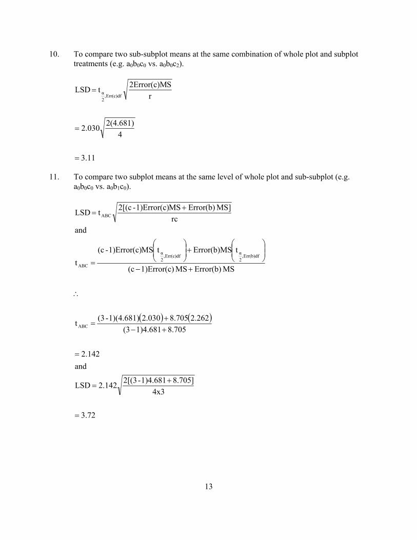
10. To compare two sub-subplot means at the same combination of whole plot and subplot treatments (e.g. a0b0c0 vs. a0b0c2).

3.11

42(4.681)2.030

rS2Error(c)M t LSD

Err(c)df,2α

=

=

=

11. To compare two subplot means at the same level of whole plot and sub-subplot (e.g.

a0b0c0 vs. a0b1c0).

( ) ( )

72.3

4x3]705.8 1)4.681-2[(3142.2LSD

and2.142

705.81)4.681(32.262705.82.0301)(4.681)-(3t

MS Error(b)MS 1)Error(c)(c

tError(b)MStMS1)Error(c)-(ct

andrc

MS] Error(b) MS1)Error(c)-2[(c t LSD

ABC

Err(b)df,2αErr(c)df,

2α

ABC

ABC

=

+=

=

+−+

=

∴

+−

+

=

+=

13

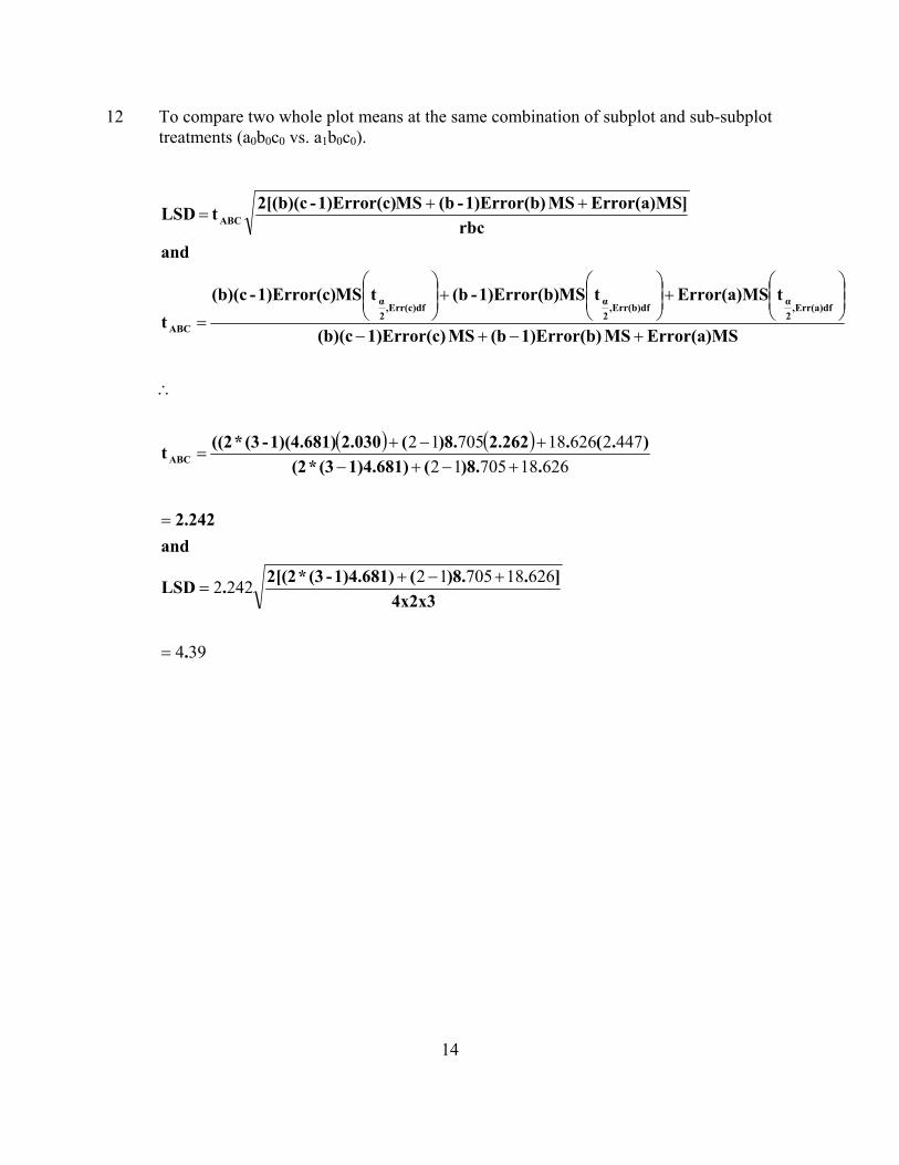
12 To compare two whole plot means at the same combination of subplot and sub-subplot treatments (a0b0c0 vs. a1b0c0).

( ) ( )

394

62618705122422

626187051244726261870512

.

4x2x3]..8)( 1)4.681)-(3*2[(2.LSD

and2.242

..8)(1)4.681)(3*(2).(.2.262.8)(2.0301)(4.681)-(3*((2t

Error(a)MSMS 1)Error(b)(bMS 1)Error(c)(b)(c

tError(a)MStMS1)Error(b)-(btMS1)Error(c)-(b)(ct

andrbc

]Error(a)MSMS 1)Error(b)-(b MS1)Error(c)-2[(b)(ct LSD

ABC

Err(a)df,2αErr(b)df,

2αErr(c)df,

2α

ABC

ABC

=

+−+=

=

+−+−+−+

=

∴

+−+−

+

+

=

++=

14