Embed Size (px)
Citation preview
Mathematische Zeitschrift (2021) 299:1351–1419https://doi.org/10.1007/s00209-021-02726-6 Mathematische Zeitschrift
Spinors of real type as polyforms and the generalized Killingequation
Vicente Cortés1 · Calin Lazaroiu2,3 · C. S. Shahbazi1
Received: 8 March 2020 / Accepted: 3 February 2021 / Published online: 19 March 2021© The Author(s) 2021
AbstractWe develop a new framework for the study of generalized Killing spinors, where everygeneralizedKilling spinor equation, possiblywith constraints, can be formulated equivalentlyas a system of partial differential equations for a polyform satisfying algebraic relations in theKähler–Atiyah bundle constructed by quantizing the exterior algebra bundle of the underlyingmanifold. At the core of this framework lies the characterization, which we develop in detail,of the image of the spinor squaring map of an irreducible Clifford module � of real type asa real algebraic variety in the Kähler–Atiyah algebra, which gives necessary and sufficientconditions for a polyform to be the square of a real spinor.We apply these results to Lorentzianfour-manifolds, obtaining a new description of a real spinor on such a manifold through acertain distribution of parabolic 2-planes in its cotangent bundle. We use this result to giveglobal characterizations of real Killing spinors on Lorentzian four-manifolds and of four-dimensional supersymmetric configurations of heterotic supergravity. In particular, we findnew families of Einstein and non-Einstein four-dimensional Lorentzian metrics admittingreal Killing spinors, some of which are deformations of the metric of AdS4 space-time.
Keywords Spin geometry · Generalized Killing spinors · Spinor bundles · Lorentziangeometry
Mathematics Subject Classification Primary 53C27; Secondary 53C50
B C. S. [email protected]
Vicente Corté[email protected]
Calin [email protected]
1 Department of Mathematics, University of Hamburg, Hamburg, Germany
2 Center for Geometry and Physics, Institute for Basic Science, Pohang, Republic of Korea
3 Department of Theoretical Physics, Horia Hulubei National Institute for Physics and NuclearEngineering, Bucharest, Romania
123
1352 V. Cortés et al.
Contents
1 Introduction . . . . . . . . . . . . . . . . . . . . . . . . . . . . . . . . . . . . . . . . . . . . . 13521.1 Background and context . . . . . . . . . . . . . . . . . . . . . . . . . . . . . . . . . . . . . 13521.2 Main results . . . . . . . . . . . . . . . . . . . . . . . . . . . . . . . . . . . . . . . . . . . 13541.3 Open problems and further directions . . . . . . . . . . . . . . . . . . . . . . . . . . . . . . 13571.4 Outline of the paper . . . . . . . . . . . . . . . . . . . . . . . . . . . . . . . . . . . . . . . 1357
2 Representing real vectors as endomorphisms in a paired vector space . . . . . . . . . . . . . . . 13582.1 Tame endomorphisms and the squaring maps . . . . . . . . . . . . . . . . . . . . . . . . . 13592.2 Admissible endomorphisms . . . . . . . . . . . . . . . . . . . . . . . . . . . . . . . . . . . 13592.3 The manifold Z and the projective squaring map . . . . . . . . . . . . . . . . . . . . . . . 13612.4 Tamings ofB . . . . . . . . . . . . . . . . . . . . . . . . . . . . . . . . . . . . . . . . . . 13622.5 Characterizations of tame admissible endomorphisms . . . . . . . . . . . . . . . . . . . . . 13632.6 Two-dimensional examples . . . . . . . . . . . . . . . . . . . . . . . . . . . . . . . . . . . 13662.7 Including linear constraints . . . . . . . . . . . . . . . . . . . . . . . . . . . . . . . . . . . 1368
3 From real spinors to polyforms . . . . . . . . . . . . . . . . . . . . . . . . . . . . . . . . . . . 13683.1 Admissible pairings for irreducible real Clifford modules . . . . . . . . . . . . . . . . . . . 13683.2 The Kähler–Atiyah model of Cl(V ∗, h∗) . . . . . . . . . . . . . . . . . . . . . . . . . . . . 13723.3 Spinor squaring maps . . . . . . . . . . . . . . . . . . . . . . . . . . . . . . . . . . . . . . 13753.4 Linear constraints . . . . . . . . . . . . . . . . . . . . . . . . . . . . . . . . . . . . . . . . 13793.5 Real chiral spinors . . . . . . . . . . . . . . . . . . . . . . . . . . . . . . . . . . . . . . . . 13793.6 Low-dimensional examples . . . . . . . . . . . . . . . . . . . . . . . . . . . . . . . . . . . 1380
3.6.1 Signature (2, 0) . . . . . . . . . . . . . . . . . . . . . . . . . . . . . . . . . . . . . . 13803.6.2 Signature (1, 1) . . . . . . . . . . . . . . . . . . . . . . . . . . . . . . . . . . . . . . 13813.6.3 Signature (3, 1) . . . . . . . . . . . . . . . . . . . . . . . . . . . . . . . . . . . . . . 13823.6.4 Signature (2, 2) . . . . . . . . . . . . . . . . . . . . . . . . . . . . . . . . . . . . . . 1385
4 Constrained generalized Killing spinors of real type . . . . . . . . . . . . . . . . . . . . . . . . 13864.1 Bundles of real simple Clifford modules . . . . . . . . . . . . . . . . . . . . . . . . . . . . 13874.2 Paired spinor bundles . . . . . . . . . . . . . . . . . . . . . . . . . . . . . . . . . . . . . . 13894.3 Constrained generalized Killing spinors . . . . . . . . . . . . . . . . . . . . . . . . . . . . 13914.4 Spinor squaring maps . . . . . . . . . . . . . . . . . . . . . . . . . . . . . . . . . . . . . . 13914.5 Description of constrained generalized Killing spinors as polyforms . . . . . . . . . . . . . 13944.6 Real spinors on Lorentzian four-manifolds . . . . . . . . . . . . . . . . . . . . . . . . . . . 13964.7 Real spinors on globally hyperbolic Lorentzian four-manifolds . . . . . . . . . . . . . . . . 1397
5 Real Killing spinors on Lorentzian four-manifolds . . . . . . . . . . . . . . . . . . . . . . . . . 13995.1 Describing real Killing spinors through differential forms . . . . . . . . . . . . . . . . . . . 14005.2 The Pfaffian system and its consequences . . . . . . . . . . . . . . . . . . . . . . . . . . . 14015.3 The locally stationary and locally integrable case . . . . . . . . . . . . . . . . . . . . . . . 14035.4 Special solutions from the Poincaré half-plane . . . . . . . . . . . . . . . . . . . . . . . . . 1406
6 Supersymmetric heterotic configurations . . . . . . . . . . . . . . . . . . . . . . . . . . . . . . 14096.1 Supersymmetric heterotic configurations . . . . . . . . . . . . . . . . . . . . . . . . . . . . 14096.2 Characterizing supersymmetric heterotic configurations through differential forms . . . . . . 14106.3 Some examples . . . . . . . . . . . . . . . . . . . . . . . . . . . . . . . . . . . . . . . . . 1412
Appendix A: Parabolic 2-planes and degenerate complete flags in R3,1 . . . . . . . . . . . . . . . . 1413
Appendix B: Heterotic supergravity in four Lorentzian dimensions . . . . . . . . . . . . . . . . . . 1414References . . . . . . . . . . . . . . . . . . . . . . . . . . . . . . . . . . . . . . . . . . . . . . . . 1417
1 Introduction
1.1 Background and context
Let (M, g) be a pseudo-Riemannian manifold of signature (p, q), equipped with a bundleof irreducible real Clifford modules S. If (M, g) admits a spin structure, then S carries acanonical connection ∇S which lifts the Levi-Civita connection of g. This allows one todefine the notions of parallel and Killing spinors, both of which were studied extensively inthe literature [8,16,58,77,88]. Developments in supergravity and differential geometry (see
123
Spinors of real type as polyforms and the generalized Killing equation 1353
references cited below) require the study of more general linear first-order partial differentialequations for spinor fields. It is therefore convenient to develop a general framework whichsubsumes all such spinorial equations as special cases. In order to do this, we assume thatS is endowed with a fixed connection D : �(S) → �(T ∗M ⊗ S) (which in practice willdepend on various geometric structures on (M, g) relevant to the specific problem underconsideration) and consider the equation:
Dε = 0 (1)
for a real spinor ε ∈ �(S). Solutions to this equation are called generalized Killing spinorswith respect toD or simplyD-parallel spinors on (M, g).We also consider linear constraintsof the form:
Q(ε) = 0, (2)
where Q ∈ �(Hom(S,W⊗ S)), withW a vector bundle defined on M . Solutions ε ∈ �(M)
of the system of Eqs. (1) and (2) are called constrained generalized Killing spinors on (M, g).The study of generalized Killing spinors can be motivated from various points of view,
such as the theory of spinors on hypersurfaces [9,23,29,33,78] or Riemannian geometrywith torsion [31,60]. There is nowadays an extensive literature on the existence and prop-erties of manifolds admitting generalized Killing spinors for specific connections D and inthe presence of various spinorial structures, see for example [2,3,32,55,57,59,76,79,80] andreferences therein.
Generalized Killing spinors play a fundamental role in supergravity and string theory[45,84,85]. They occur in these physics theories through the notion of “supersymmetric con-figuration”, whose definition involves spinors parallel under a connection D on S which isparameterized by geometric structures typically defined on fiber bundles, gerbes or Courantalgebroids associated to (M, g) [28,51,81]. This produces the notion of supergravity Killingspinor equations—particular instances of (systems of) constrained generalizedKilling spinorequations which are specific to the physics theory under consideration. Pseudo-Riemannianmanifolds endowedwith parameterizing geometric structures for which such equations admitnon-trivial solutions are called supersymmetric configurations. They are called supersymmet-ric solutions if they also satisfy the equations of motion of the given supergravity theory. Thestudy of supergravity Killing spinor equations was pioneered by Tod [84,85] and later devel-oped systematically in several references, including [7,10,11,19,27,40–43,63–66,70,71]. Thestudy of supersymmetric solutions of supergravity theories provided an enormous boost to thesubject of generalized Killing spinors and to spinorial geometry as a whole, which resultedin a large body of literature both in physics and mathematics, the latter of which is largelydedicated to the case of Euclidean signature in higher dimensional theories. We refer thereader to [1,26,31,38,51,81] and references therein for more details and exhaustive lists ofreferences.
Supergravity Killing spinor equations pose a number of new challenges when comparedto simpler spinorial equations traditionally considered in the mathematics literature. First,supergravity Killing spinor equations must be studied for various theories and in variousdimensions and signatures (usually Riemannian and Lorentzian), for real as well as complexspinors. In particular, this means that every single case in the modulo eight classificationof real Clifford algebras must be considered, adding a layer of complexity to the problem.Second, such equations involve spinors parallel under non-canonical connections coupledto several other objects such as connections on gerbes, principal bundles or maps from theunderlyingmanifold into a Riemannianmanifold of special type. These objects, together with
123
1354 V. Cortés et al.
the underlying pseudo-Riemannian metric, must be treated as parameters of the supergravityKilling spinor equations, yielding a highly nontrivial non-linearly coupled system.Moreover,the formulation of supergravity theories relies on the Dirac–Penrose1 rather than on theCartan approach to spinors. As a result, spinors appearing in such theories need not beassociated to a spin structure or other a priory classical spinorial structure but involve themore general concept of a (real or complex) Lipschitz structure (see [35,67–69]). The latternaturally incorporates the ‘R-symmetry’ groupof the theory and is especiallywell-adapted forgeometric formulations of supergravity. Third, applications require the study of the modulispace of supersymmetric solutions of supergravity theories, involving the metric and allother geometric objects entering their formulation. This set-up yields remarkably nontrivialmoduli problems for which the automorphism group(oid) of the system is substantially morecomplicated than the more familiar infinite-dimensional gauge group of automorphisms ofa principal bundle or the diffeomorphism group of a compact manifold. Given these aspects,the study of supergravity Killing spinor equations and of moduli spaces of supersymmetricsolutions of supergravity theories requires methods and techniques specifically dedicated totheir understanding [22,38,42,48,52–54,63,66–70]. Developing suchmethods in a systematicmanner is one of the goals of this article.
1.2 Main results
One approach to the study of supergravity Killing spinor equations is the so-called “methodof bilinears” [42,84,85], which was successfully applied in various cases to simplify thelocal partial differential equations characterizing certain supersymmetric configurations andsolutions. The idea behind this method is to consider the polyform constructed by takingthe ‘square’ of the Killing spinor (instead of the spinor itself) and use the correspondingconstrained generalized Killing spinor equations to extract a system of algebraic and partialdifferential equations for this polyform, thus producingnecessary conditions for a constrainedgeneralizedKilling spinor to exist on (M, g). These conditions can also be exploited to obtaininformation on the structure of supersymmetric solutions of the supergravity theory at hand.The main goal of the present work is to develop a framework inspired by these ideas aimedat investigating constrained generalized Killing spinors on pseudo-Riemannian manifolds byconstructing a mathematical equivalence between real spinors and their polyform squares.
Whereas the fact that the ‘square of a spinor’ [5,15,56] (see Definition 3.16 in Sect. 3)yields a polyform has been known for a long time (and the square of certain spinors withparticularly nice stabilizers is well-known in specific—usually Riemannian—cases [15]),a proper mathematical theory to systematically characterize and compute spinor squaresin every dimension and signature has been lacking so far. In this context, the fundamentalquestions to be addressed are2:
(1) What are the necessary and sufficient conditions for a polyform to be the square of aspinor, in every dimension and signature?
1 When constructing such theories, one views spinors as sections of given bundles of Clifford modules. Theexistence of such bundles on the given space-time is postulated when writing down the theory, rather thandeduced through the associated bundle construction from a specific classical spinorial structure assumed onto exist on that spacetime.2 A systematic approach of this type was first used in references [64,65] for generalized Killing spinor equa-tions in certain 8-dimensional flux compactifications of M-theory, using the Kähler–Atiyah bundle approachto such problems developed previously in [63,66,70].
123
Spinors of real type as polyforms and the generalized Killing equation 1355
(2) Canwe (explicitly, if possible) translate constrainedgeneralizedKilling spinor equationsinto equivalent algebraic and partial differential equations for the square polyform?
In this work, we solve both questions for irreducible real spinors when the signature(p, q) of the underlying pseudo-Riemannian manifold satisfies p− q ≡8 0, 2, i.e. when thecorresponding Clifford algebra is simple and of real type. We solve question (1) by fullycharacterizing the space of polyforms which are the (signed) square of spinors as the set ofsolutions of a system of algebraic equations which define a real affine variety in the spaceof polyforms. Every polyform solving this algebraic system can be written as the square ofa real spinor which is determined up to a sign factor—and vice-versa. Following [63,66,70],the aforementioned algebraic system can be neatly written using the geometric product.The latter quantizes the wedge product, thereby deforming the exterior algebra to a unitalassociative algebra which is isomorphic to the Clifford algebra. This algebraic system canbe considerably more complicated in indefinite signature than in the Euclidean case. On theother hand, we solve question (2) in the affirmative by reformulating constrained generalizedKilling spinor equations on a spacetime (M, g) of such signatures (p, q) as an equivalentsystem of algebraic and partial differential equations for the square polyform. Altogether, thisproduces an equivalent reformulationof the constrainedgeneralizedKilling spinor problemasa more transparent and easier to handle system of partial differential equations for a polyformsatisfying certain algebraic equations in the Kähler–Atiyah bundle of (M, g). We believe thatthe framework developed in this paper is especially useful in pseudo-Riemannian signatureand in higher dimensions, where the spin group does not act transitively on the unit spherein spinor space and hence representation theory cannot be easily exploited to understandthe square of a spinor in purely representation theoretic terms. One of our main results (seeTheorem 4.26 for details and notation) is:
Theorem 1.1 Let (M, g) be a connected, oriented and strongly spin pseudo-Riemannianmanifold of signature (p, q) and dimension d = p+ q, such that p− q ≡8 0, 2. LetW be avector bundle on M and (S, �,B ) be a paired real spinor bundle on (M, g)whose admissiblepairing has symmetry and adjoint types σ, s ∈ {−1, 1}. Fix a connection D = ∇S −A on S(whereA ∈ �1(M, End(S))) and amorphism of vector bundlesQ ∈ �(End(S)⊗W). Thenthere exists a nontrivial generalized Killing spinor ε ∈ �(S) with respect to the connectionD which also satisfies the linear constraint Q(ε) = 0 iff there exists a nowhere-vanishingpolyform α ∈ �(M) which satisfies the following algebraic and differential equations:
α � β � α = 2d2 (α � β)(0) α, (π
1−s2 ◦ τ)(α) = σ α, (3)
∇gα = A � α + α � (π 1−s2 ◦ τ)(A), Q � α = 0 (4)
for every polyform β ∈ �(M), where A ∈ �1(M,∧T ∗M) and Q ∈ �(∧T ∗M⊗W) are thesymbols of A and Q while π , τ are the canonical automorphism and anti-automorphism ofthe Kähler–Atiyah bundle (∧T ∗M,�) of (M, g). If ε is chiral of chirality μ ∈ {−1, 1}, thenwe have to add the condition:
∗(π ◦ τ)(α) = μα,
where ∗ is the Hodge operator of (M, g). Moreover, any such polyform α determines anowhere-vanishing real spinor ε ∈ �(S), which is unique up to a sign and satisfies theconstrained generalized Killing spinor equations with respect to D and Q.
123
1356 V. Cortés et al.
When (M, g) is a Lorenzian four-manifold, we say that a pair of nowhere-vanishing one-forms (u, l) defined on M is parabolic if u and l are mutually orthogonal with u null andl spacelike of unit norm. Applying the previous result, we obtain (see Theorem 4.32 andSect. 4.6 for detail and terminology):
Theorem 1.2 Let (M, g) be a connected and spin Lorentzian four-manifold of “mostly plus”signature such that H1(M,Z2) = 0 and S be a real spinor bundle associated to the spinstructure of (M, g) (which is unique up to isomorphism). Then there exists a natural bijec-tion between the set of global smooth sections of the projective bundle P(S) and the set oftrivializable and co-oriented distributions (�,H) of parabolic 2-planes in T ∗M. Moreover,there exist natural bijections between the following two sets:
(a) The set �(S)/Z2 of sign-equivalence classes of nowhere-vanishing real spinors ε ∈�(S).
(b) The set of strong equivalence classes of parabolic pairs of one-forms (u, l) ∈ P(M, g).
In particular, the sign-equivalence class of a nowhere-vanishing spinor ε ∈ �(S) determinesand is determined by a parabolic pair of one-forms (u, l) considered up to transformationsof the form (u, l)→ (−u, l) and l → l + cu with c ∈ R.
Weuse this result to characterize spinLorentzian four-manifolds (M, g)with H1(M, g) =0 which admit real Killing spinors and supersymmetric bosonic heterotic configurationsassociated to “paired principal bundles” (P, c) over such a manifold through systems ofpartial differential equations for u and l, which we explore in specific cases. Taking (M, g)to be of signature (3, 1), we prove the following results (see Theorems 5.3 and 6.6), where ∗and d∗ denote the Hodge operator and codifferential of (M, g) while ∇g denotes the actionof its Levi-Civita on covariant tensors:
Theorem 1.3 (M, g) admits a nontrivial real Killing spinor with Killing constant λ2 ∈ R iff
it admits a parabolic pair of one-forms (u, l) which satisfies:
∇gu = λ u ∧ l, ∇gl = λ (l ⊗ l − g)+ κ ⊗ u
for some κ ∈ �1(M). In this case, u� ∈ X(M) is a Killing vector field with geodesic integralcurves.
Theorem 1.4 A bosonic heterotic configuration (g, ϕ, H , A) of (M, P, c) is supersymmetric
iff there exists a parabolic pair of one-forms (u, l)which satisfies (here ρdef.= ∗H ∈ �1(M)):
ϕ ∧ u = ∗(ρ ∧ u), ϕ ∧ u ∧ l = −g∗(ρ, l) ∗ u, − g∗(ϕ, l) u = ∗(l ∧ u ∧ ρ),
g∗(u, ϕ) = 0, g∗(u, ρ) = 0, g∗(ρ, ϕ) = 0, FA = u ∧ χA,
∇gu = 1
2u ∧ ϕ, ∇gl = 1
2∗ (ρ ∧ l)+ κ ⊗ u, d∗ρ = 0
for some one-form κ ∈ �1(M) and some gP-valued one-form χA ∈ �1(M, gP ) which isorthogonal to u. In this case, u� ∈ X(M) is a Killing vector field.
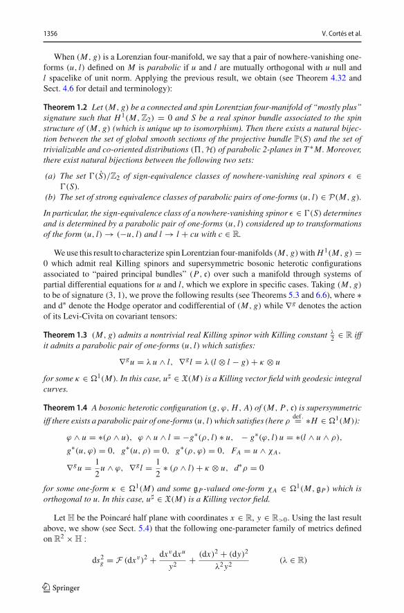
Let H be the Poincaré half plane with coordinates x ∈ R, y ∈ R>0. Using the last resultabove, we show (see Sect. 5.4) that the following one-parameter family of metrics definedon R
2 ×H :
ds2g = F (dxv)2 + dxvdxu
y2+ (dx)2 + (dy)2
λ2y2(λ ∈ R)
123
Spinors of real type as polyforms and the generalized Killing equation 1357
(where R2 has Cartesian coordinates xv, xu) admits real Killing spinors for every F ∈
C∞(H). We also show that these metrics are Einstein with Einstein constant � = −3λ2when F has the form:
F = (a1 + a2x)
(a3y + a4
y2
)or F = (a1e
cx + a2e−cx ) [a3BY(cy)+ a4BJ(cy)] ,
where BY and BJ are the spherical Bessel functions and a1, . . . , a4 ∈ R. These give defor-mations of the AdS4 spacetime of cosmological constant �, which obtains for a1 = a2 =a3 = a4 = 0.
1.3 Open problems and further directions
Theorem 1.1 refers exclusively to real spinors in signature p − q ≡8 0, 2, for which theirreducible Clifford representation map is an isomorphism. It would be interesting to extendthis result to the remaining signatures, which encompass twomain cases, namely real spinorsof complex andquaternionic type (the latter ofwhich canbe reducible). Thiswould yield a richreformulation of the theory of real spinors through polyforms subject to algebraic constraints,which could be used to study generalized Killing spinors in all dimensions and signatures. Itwould also be interesting to extend Theorem 1.1 to other types of spinorial equations, suchas those characterizing harmonic or twistor spinors and generalizations thereof, investigatingif it is possible to develop an equivalent theory exclusively in terms of polyforms.
Some important signatures satisfy the condition p − q ≡8 0, 2, most notably signatures(2, 0), (1, 1), (3, 1) and (9, 1). The latter two are especially relevant to supergravity theo-ries and one could apply the formalism developed in this article to study moduli spaces ofsupersymmetric solutions in these cases. Several open problems of analytic, geometric andtopological type exist regarding the heterotic system in four and ten Lorentzian dimensions,as the mathematical study of its Riemannian analogue shows [38]. Most problems related toexistence, classification, construction of examples and moduli are open and give rise to inter-esting analytic and geometric questions on Lorentzian four-manifolds and ten-manifolds.In this direction, we hope that Appendix B can serve as a brief introduction to heteroticsupergravity in four Lorentzian dimensions for mathematicians who may be interested insuch questions. The local structure of ten-dimensional supersymmetric solutions to heteroticsupergravity was explored in [49,50,82], where that problem was reduced to a minimal setof partial differential equations on a local Lorentzian manifold of special type.
1.4 Outline of the paper
Section 2 gives the description of rank-one endomorphisms of a vector space which are (anti-)symmetric with respect to a non-degenerate bilinear pairing assumed to be symmetric orskew-symmetric. Section 3 develops the algebraic theory of the square of a spinor culminatingin Theorem 3.20, which characterizes it through a system of algebraic conditions in theKähler–Atiyah algebra of the underlying quadratic vector space. In Sect. 4, we apply thisto real spinors on pseudo-Riemannian manifolds of signature (p, q) satisfying p − q ≡8
0, 2, obtaining a complete characterization of generalized constrained Killing spinors aspolyforms satisfying algebraic and partial differential equations which we list explicitly.Section 5 applies this theory to real Killing spinors in four Lorentzian dimensions, obtaininga new global characterization of such. In Sect. 6, we apply the same theory to the study of
123
1358 V. Cortés et al.
supersymmetric configurations of heterotic supergravity, whose mathematical formulation isexplained briefly in an appendix.Notations and conventions Throughout the paper, we use Einstein summation over repeatedindices. We let R× denote the group of invertible elements of any commutative ring R. Inparticular, the multiplicative group of non-zero real numbers is denoted by R
× = R. For anypositive integer n, the symbol≡n denotes the equivalence relation of congruence of integersmodulo n, while Zn = Z/nZ denotes the corresponding congruence group. All manifoldsconsidered in the paper are assumed to be smooth, connected and paracompact, while allfiber bundles are smooth. The set of globally-defined smooth sections of any fiber bundle Fdefined on a manifold M is denoted by �(F). We denote by G0 the connected component ofthe identity of any Lie group G. Given a vector bundle S on a manifold M , the dual vectorbundle is denoted by S∗ while the bundle of endomorphisms is denoted by End(S) � S∗⊗S.The trivial real line bundle on M is denoted by RM . The space of globally-defined smoothsections of S is denoted by �(S), while the set of those globally-defined smooth sections of S
which do not vanish anywhere onM is denoted by·�(S). The complement of the origin in any
R-vector space� is denoted by � while the complement of the image 0S of the zero section
of a vector bundle S defined on a manifold M is denoted by S. The inclusion·�(S) ⊂ ·
�(S)is generally strict. If A is any subset of the total space of S, we define:
�(A)def.= {s ∈ �(S) | sm ∈ A ∩ Sm ∀m ∈ M} ⊂ �(S). (5)
Notice the relation·�(S) = �(S). All pseudo-Riemannian manifolds (M, g) are assumed to
have dimension at least two and signature (p, q) satisfying p − q ≡8 0, 2; in particular, allLorentzian four-manifolds have “mostly plus” signature (3, 1). For any pseudo-Riemannianmanifold (M, g), we denote by 〈, 〉g the (generally indefinite) metric induced by g on the
total exterior bundle�(M)def.= ∧T ∗M = ⊕dim M
k=0 ∧k T ∗M . We denote by∇g the Levi-Civitaconnection of g and use the same symbol for its action on tensors. The equivalence class of anelement ξ of an R-vector space � under the sign action of Z2 on � is denoted by ξ ∈ �/Z2
and called the sign equivalence class of ξ .
2 Representing real vectors as endomorphisms in a paired vector space
Let � be an R-vector space of positive even dimension N ≥ 2, equipped with a non-degenerate bilinear pairing B : � × � → R, which we assume to be either symmetric orskew-symmetric. In this situation, the pair (�,B ) is called a paired vector space. We saythat B (or (�,B )) has symmetry type σ ∈ {−1, 1} if:
B (ξ1, ξ2) = σB (ξ2, ξ1) ∀ ξ1, ξ2 ∈ �.
Thus B is symmetric if it has symmetry type +1 and skew-symmetric if it has symmetrytype−1. Let (End(�), ◦) be the unital associative R-algebra of linear endomorphisms of�,where ◦ denotes composition of linear maps. Given E ∈ End(�), let Et ∈ End(�) denotethe adjoint of E taken with respect to B , which is uniquely determined by the condition:
B (ξ1, E(ξ2)) = B (Et (ξ1), ξ2) ∀ξ1, ξ2 ∈ �.
The map E → Et is a unital anti-automorphism of the R-algebra (End(�), ◦).
123
Spinors of real type as polyforms and the generalized Killing equation 1359
2.1 Tame endomorphisms and the squaringmaps
Definition 2.1 An endomorphism E ∈ End(�) is called tame if its rank satisfies rk(E) ≤ 1.
Thus E is tame iff it vanishes or is of unit rank. Let:
T := T (�)def.= {E ∈ End(�) | rk(E) ≤ 1} ⊂ End(�)
be the real determinantal variety of tame endomorphisms of � and:
T := T (�)def.= T \ {0} = {E ∈ End(�) | rk(E) = 1}
be its open subset consisting of endomorphisms of rank one. We view T as a real affinevariety of dimension 2N − 1 in the vector space End(�) � R
N2and T as a semi-algebraic
variety. Elements of T can be written as:
E = ξ ⊗ β,
for some ξ ∈ � and β ∈ �∗, where �∗ = Hom(�,R) denotes the vector space dual to �.Notice that tr(E) = β(ξ). When E ∈ T is non-zero, the vector ξ and the linear functionalβ appearing in the relation above are non-zero and determined by E up to transformationsof the form (ξ, β)→ (λξ, λ−1β) with λ ∈ R
×. In particular, T is a manifold diffeomorphicwith the quotient (RN \ {0})× (RN \ {0})/R×, where R
× acts with weights +1 and −1 onthe two copies of R
N \ {0}.Definition 2.2 The signed squaring maps of a paired vector space (�,B ) are the quadraticmaps E± : �→ T defined through:
E±(ξ) = ±ξ ⊗ ξ∗ ∀ξ ∈ �,
where ξ∗ def.= B (−, ξ) ∈ �∗ is the linear map dual to ξ relative to B . The map E+ is calledthe positive squaring map of (�,B ), while E− is called the negative squaring map of(�,B ).
Let κ ∈ {−1, 1} be a sign factor and consider the open semi-algebraic set �def.= �\ {0}.
Notice that E±(ξ) = 0 iff ξ = 0, hence E±(�) ⊂ T . Let E± : � → T be the restrictions ofE± to �. The proof of the following lemma is immediate.
Lemma 2.3 For each κ ∈ {−1, 1}, the restricted quadratic map Eκ : � → T is two-to-one,namely:
E−1κ ({κ ξ ⊗ ξ∗}) = {−ξ, ξ} ∀ξ ∈ �.
Moreover, we have Eκ (ξ) = 0 iff ξ = 0 and hence Eκ is a real branched double cover of itsimage, which is ramified at the origin.
2.2 Admissible endomorphisms
The maps E± need not be surjective. To characterize their images, we introduce the notionof admissible endomorphism. Let (�,B ) be a paired vector space of type σ .
Definition 2.4 An endomorphism E of� is calledB -admissible if it satisfies the conditions:
E ◦ E = tr(E)E and Et = σ E .
123
1360 V. Cortés et al.
Let:
C := C(�,B )def.= {
E ∈ End(�) | E ◦ E = tr(E)E, Et = σ E}
denote the real cone of B -admissible endomorphisms of �.
Remark 2.5 Tame endomorphisms are not related to admissible endomorphisms in any simpleway. A tame endomorphism need not be admissible, since it need not be (anti-)symmetricwith respect to B . An admissible endomorphism need not be tame, since it can have ranklarger than one (as shown by a quick inspection of explicit examples in four dimensions).
Let:
Z := Z(�,B )def.= T (�) ∩ C(�,B ) (6)
denote the real cone of those endomorphisms of E which are both tame and B -admissible
and consider the open set Z def.= Z\ {0}.Lemma 2.6 We have:
Z = Im(E+) ∪ Im(E−) and Im(E+) ∩ Im(E−) = {0}.Hence an endomorphism E ∈ End(�) belongs to Z iff there exists a non-zero vector ξ ∈ �
and a sign factor κ ∈ {−1, 1} such that:
E = Eκ (ξ).
Moreover, κ is uniquely determined by E through this equation while ξ is determined up tosign.
Proof Let E ∈ Z . Since E has unit rank, there exists a non-zero vector ξ ∈ � and a non-zerolinear functional β ∈ �∗ such that E = ξ ⊗ β. Since B is non-degenerate, there exists aunique non-zero ξ0 ∈ � such that β = B (−, ξ0) = ξ∗0 . The condition Et = σ E amountsto:
B (−, ξ0)ξ = B (−, ξ)ξ0.SinceB is non-degenerate, there exists χ ∈ � such thatB (χ, ξ) �= 0, which by the previousequations also satisfies B (χ, ξ0) �= 0. Hence:
ξ0 = B (χ, ξ0)
B (χ, ξ)ξ = B (ξ0, χ)
B (ξ, χ)ξ
and:
E = B (ξ0, χ)
B (ξ, χ)ξ ⊗ ξ∗.
Using the rescaling ξ �→ ξ ′ def.=∣∣∣∣B (ξ0,χ)B (ξ,χ)
∣∣∣∣12
ξ , the previous relation gives E = κ ξ ′ ⊗ (ξ ′)∗ ∈Im(Eκ ), where κ
def.= sign(B (ξ0,χ)B (ξ,χ)
). This implies the inclusion Z ⊆ Im(E+) ∪ Im(E−).
Lemma 2.3 now shows that ξ ′ is unique up to sign. The inclusion Im(E+) ∪ Im(E−) ⊆ Zfollows by direct computation using the explicit form E = κ ξ ⊗ ξ∗ of an endomorphismE ∈ Im(Eκ ), which implies:
E ◦ E = B (ξ, ξ)E, Et = σ E, tr(E) = B (ξ, ξ).
123
Spinors of real type as polyforms and the generalized Killing equation 1361
Combining the two inclusions above gives Z = Im(E+) ∪ Im(E−). The relation Im(E+) ∩Im(E−) = {0} follows immediately from Lemma 2.3. ��Definition 2.7 The signature κE ∈ {−1, 1} of an element E ∈ Z with respect to B is thesign factor κ determined by E as in Lemma 2.6. When E = 0, we set κE = 0.
Remark 2.8 Notice that κ−E = −κE for all E ∈ Z.
In view of the above, define:
Z± := Z±(�,B )def.= Im(E±). (7)
Then:
Z− = −Z+, Z = Z+ ∪ Z− and Z+ ∩ Z− = {0}.Let Z2 � {−1, 1} act on � and on Z ⊂ End(E) by sign multiplication. Then E+ and E−induce the same map between the quotients (which is a bijection by Lemma 2.6). We denotethis map by:
E : �/Z2∼→ Z/Z2. (8)
Definition 2.9 The bijection (8) is called the class squaring map of (�,B ).
2.3 Themanifold Z and the projective squaringmap
Given any endomorphism A ∈ End(�), define a (possibly degenerate) bilinear pairing B A
on � through:
B A(ξ1, ξ2)def.= B (ξ1, A(ξ2)) ∀ξ1, ξ2 ∈ �. (9)
Notice that B A is symmetric iff At = σ A and skew-symmetric iff At = −σ A.
Proposition 2.10 The open set Z has two connected components, which are given by:
Z+def.= Im(E+) = Im(E+) \ {0} and Z−
def.= Im(E−) = Im(E−) \ {0},and satisfy:
Z+ = {E ∈ Z|κE = +1} ⊂ {E ∈ Z | B E ≥ 0} ,Z− = {E ∈ Z|κE = −1} ⊂ {E ∈ Z | B E ≤ 0} .
Moreover, the maps E± : �→ Z± define principal Z2-bundles over Z±.
Proof By Lemma 2.6, we know that Z = Z+ ∪ Z− and Z+ ∩ Z− = ∅. The open set � isconnected because N = dim� ≥ 2. Fix κ ∈ {−1, 1}. Since the continuous map Eκ surjectsonto Zκ , it follows that Zκ is connected. Let E ∈ Zκ . The pairing B E is symmetric sinceEt = σ E . By Lemma 2.6, we have E = κ B (−, ξ0)ξ0 for some non-zero ξ0 ∈ � and hence:
B E (ξ, ξ) = B (ξ, E(ξ)) = κ|B (ξ, ξ0)|2 ∀ ξ ∈ �.
Since ξ0 �= 0 and B is non-degenerate, this shows that B E is nontrivial and that it ispositive-semidefinite when restricted to Z+ and negative-semidefinite when restricted toZ−. The remaining statement follows from Lemmas 2.3 and 2.6. ��
123
1362 V. Cortés et al.
Proposition 2.11 Z(�,B ) is amanifold diffeomorphic toR××RP
N−1 (where N = dim�).
Proof Let | · |20 denotes the norm induced by any scalar product on �. Then the diffeomor-phism:
Z ∼−→ R× × RP
N−1, κ ξ ⊗ ξ∗ �→ (κ |ξ |20, [ξ ])satisfies the desired properties. ��
The maps E± : �→ End(�) \ {0} induce the same map:
PE : P(�)→ P(End(�)), [ξ ] �→ [ξ ⊗ ξ∗],between the projectivizations P(�) and P(End(�)) of the real vector spaces� and End(�).
Setting PZ(�,B )def.= Z(�,B )/R× ⊂ PEnd(�), Proposition 2.11 gives:
Proposition 2.12 The map PE : P(�)→ PZ(�,B ) is a diffeomorphism.
Definition 2.13 PE : P(�)∼→ PZ(�,B ) is called the projective squaring map of (�,B ).
2.4 Tamings ofB
The bilinear formB A defined in Eq. (9) is non-degenerate iff the endomorphism A ∈ End(�)
is invertible. The following result is immediate:
Proposition 2.14 Let B ′ be a non-degenerate symmetric pairing on �. Then there exists aunique endomorphism A ∈ GL(E) (called the operator ofB ′ with respect toB ) such thatB ′ = B A. Moreover, A is invertible and satisfies At = σ A. Furthermore, the transpose ET
of any endomorphism E ∈ End(�) with respect to B ′ is given by:
ET = (A−1)t Et At = A−1Et A (10)
and in particular we have AT = At = σ A.
Remark 2.15 Replacing ξ2 by A−1ξ2 in the relation B ′(ξ1, ξ2) = B (ξ1, Aξ2) gives:
B (ξ1, ξ2) = B ′(ξ1, A−1ξ2), (11)
showing that A−1 is the operator of B with respect to B ′.
Definition 2.16 We say that A ∈ End(�) is a taming of B if B A is a scalar product.
Let A ∈ End(�) be a taming ofB and denote by (−,−) def.= B A the corresponding scalarproduct. Relation (11) shows that the matrix B ofB with respect to a ( , )-orthonormal basis{e1, . . . , eN } of � is the inverse of the matrix A of A in the the same basis. Distinguish thecases:
1. WhenB is symmetric, its operator B with respect to ( , ) and the taming A = B−1 ofBare ( , )-symmetric and can be diagonalized by a (−,−)-orthogonal linear transformationof �. If (p, q) is the signature of B , Sylvester’s theorem shows that we can choose thebasis {ei } such that:
A = diag(+1, . . . ,+1,−1, . . . ,−1),with p positive and q negative entries. With this choice, we have A2 = Id.
123
Spinors of real type as polyforms and the generalized Killing equation 1363
2. When B is skew-symmetric, we have:
B (ξ1, ξ2) = −(ξ1, J (ξ2)), i.e. (ξ1, ξ2) = B (ξ1, J (ξ2)),
where J is a (−,−)-compatible complex structure on�. This gives A−1 = −J and henceA = J , which is antisymmetric with respect to both (−,−) and B . Setting N = 2n,we can choose {e1, . . . , en} to be a basis of � over C which is orthonormal with respectto the Hermitian scalar product defined by (−,−) and J and take en+i = Jei for alli = 1, . . . , n. Then the basis {e1, . . . , eN } over R is (−,−)-orthonormal while being aDarboux basis for B and we have:
A = J =[
0 In−In 0
],
where In is the identity matrix of size n.
Proposition 2.17 Let B ′ be a non-degenerate symmetric pairing on �, A be its operatorwith respect to B and E ∈ End(�) be an endomorphism of �. Then the endomorphism
EAdef.= E ◦ A ∈ End(�) is B ′-admissible iff the following relations hold:
Et = σ E and E ◦ A ◦ E = tr(E ◦ A)E . (12)
Proof Let T denote transposition of endomorphisms with respect to B ′. By definition, EA
is B ′-admissible if:
ETA = EA and E2
A = tr(EA)EA. (13)
Since A is invertible, the second of these conditions amounts to the second relation in (12).On the other hand, we have:
ETA = (E A)T = AT ET = At = At (A−1)t Et At = Et At = σ Et A,
where we used Proposition 2.14. Hence the first condition in (13) is equivalent with σ Et A =E A, which in turn amounts to Et = σ E since A is invertible. ��
2.5 Characterizations of tame admissible endomorphisms
The following gives an open subset of the cone C of admissible endomorphisms whichconsists of rank one elements.
Proposition 2.18 Let E ∈ C(�,B ) be a B -admissible endomorphism of �. If tr(E) �= 0,then E is of rank one.
Proof Define Pdef.= E
tr(E). Then P2 = P (which implies rk(P) = tr(P)) and tr(P) = 1,
whence rk(E) = rk(P) = tr(P) = 1. ��Define
K0def.= {ξ ∈ � | B (ξ, ξ) = 0} , Kμ
def.= {ξ ∈ � | B (ξ, ξ) = μ} ,where μ ∈ {−1,+1}. When B is symmetric, the set K0 ⊂ � is the isotropic cone ofB and Kμ are the positive and negative unit “pseudo-spheres” defined by B . When B isskew-symmetric, we have K0 = � and Kμ = ∅. Lemma 2.6 and Proposition 2.18 imply:
123
1364 V. Cortés et al.
Corollary 2.19 Assume that B is symmetric (i.e. σ = +1). For any μ ∈ {−1, 1}, the setE+(Kμ) ∪ E−(Kμ) is the real algebraic submanifold of End(�) given by:
E+(Kμ) ∪ E−(Kμ) ={E ∈ End(�) | E ◦ E = μ E, Et = E, tr(E) = μ
}.
Proposition 2.20 IfB is a scalar product, then every non-zeroB -admissible endomorphismE ∈ C \ {0} is tame, whence Z = C. In this case, the signature of E with respect to B isgiven by:
κE = sign(tr(E)). (14)
Proof Let E ∈ C. By Proposition 2.18, the first statement follows if we can show thattr(E) �= 0 when E �= 0. Since E is admissible, it is symmetric with respect to the scalarproduct B and hence diagonalizable with eigenvalues λ1, . . . , λN ∈ R. Taking the trace ofequation E2 = tr(E) E gives:
tr(E)2 =N∑i=1
λ2i .
Since the right-hand side is a sum of squares, it vanishes iff λ1 = · · · = λN = 0, i.e. iffE = 0. This proves the first statement. To prove the second statement, recall from Lemma 2.6that any non-zero tame admissible endomorphism E has the form E = κEξ ⊗ ξ∗ for someξ ∈ �. Taking the trace of this relation gives:
tr(E) = κEξ∗(ξ) = κEB (ξ, ξ),
which implies (14) since B (ξ, ξ) > 0. ��A quick inspection of examples shows that there exist nontrivial admissible endomor-
phisms which are not tame (and thus satisfy tr(E) = 0) as soon as there exists a totallyisotropic subspace of � of dimension at least two. In these cases we need to impose furtherconditions on the elements of C in order to guarantee tameness. To describe such conditions,we consider the more general equation:
E ◦ A ◦ E = tr(A ◦ E)E ∀ A ∈ End(�),
which is automatically satisfied by every E ∈ Im(E+) ∪ Im(E−).
Proposition 2.21 The following statements are equivalent for any endomorphism E ∈ Cwhich satisfies the condition Et = σ E:
(a) E is B -admissible and rk(E) = 1.(b) We have E2 = tr(E)E and there exists an endomorphism A ∈ End(�) satisfying:
E ◦ A ◦ E = tr(E ◦ A)E and tr(E ◦ A) �= 0. (15)
(c) E �= 0 and the relation:
E ◦ A ◦ E = tr(E ◦ A)E, (16)
is holds for every endomorphism A ∈ End(�).
Proof We first prove the implication (b)⇒ (a). By Proposition 2.18, it suffices to considerthe case tr(E) = 0. Assume A ∈ End(�) satisfies (15). Define:
Aε = Id+ ε
tr(E ◦ A) A,
123
Spinors of real type as polyforms and the generalized Killing equation 1365
where ε ∈ R>0 is a positive constant. For ε > 0 small enough, Aε is invertible and the
endomorphism Eεdef.= E ◦ Aε has non-vanishing trace given by tr(Eε) = ε. The first relation
in (15) gives:
Eε ◦ Eε = εEε .
Hence Pdef.= 1
εEε satisfies P2 = P and tr(P) = 1, whence rk(Eε) = rk(P) = 1. Since Aε
is invertible, this implies rk(E) = 1 and hence (a) holds.The implication (a) ⇒ (c) follows directly from Lemma 2.6, which shows that E ∈
Im(Eκ ) for some sign factor κ . For the implication (c)⇒ (b), notice first that setting A = Idin (16) gives E2 = tr(E). Non-degeneracy of the bilinear form induced by the trace on thespace End(�) now shows that we can choose A in Eq. (16) such that tr(E ◦ A) �= 0. ��
Proposition 2.22 Let A be a taming of B and let B ′ def.= B A be the corresponding scalarproduct on �. Then the following statements are equivalent for any endomorphism E ∈End(�):
(a) E is B -admissible and rk(E) = 1.(b) E satisfies Et = σ E as well as conditions (15) with respect to A.
In this case, there exists a non-zero vector ξ ∈ � such that:
E = κ ξ ⊗ ξ∗ = κ ′ ξ ⊗ ξ∨,
where ξ∨ = σξ∗ ◦ A denotes the linear functional dual to ξ with respect B ′ while:
κ ′ = sign(tr(E ◦ A)) ∈ {−1, 1}is the signature of E ◦ A with respect to B ′ and:
κ = σ κ ′ = σ sign(tr(E ◦ A)) ∈ {−1, 1} (17)
is the signature of E with respect to B .
Proof Set EAdef.= E ◦ A. To prove the implication (a)⇒ (b), assume that E isB -admissible
and of rank one. Then Proposition 2.21 shows that we have E ◦ A ◦ E = tr(E ◦ A)E .Since A is B -admissible, we also have Et = σ E . It follows that EA is B ′-admissible byProposition 2.17. SinceB ′ is a scalar product, Proposition 2.20 implies that EA is tame andhence tr(EA) �= 0 since EA is non-zero. Thus tr(E ◦ A) �= 0. Combining everything, thisshows that (b) holds.
To prove the implication (b) ⇒ (a), assume that E satisfies Et = σ E as well as (15).By Proposition 2.17, this implies that EA is B ′-admissible. Since tr(EA) = tr(E ◦ A) �= 0,Proposition 2.18 implies rk(EA) = 1. Hence EA is nonzero, tame and admissible withrespect to the scalar productB ′. We thus have EA = κ ′ξ ⊗ ξ∨, where κ ′ = sign(tr(EA)) =sign(tr(E ◦ A)) (see Proposition 2.20) and ξ ∈ � is a non-zero vector. Here ξ∨ ∈ �∗ is thedual of ξ with respect to B ′, which is given by:
ξ∨(ξ ′) def.= B ′(ξ ′, ξ) = B (ξ ′, Aξ) = B (Atξ ′, ξ) = ξ∗(Atξ ′) = σξ∗(Aξ ′),
i.e. ξ∨ = σξ∗ ◦ A. Thus E ◦ A = EA = σκAξ ⊗ ξ∗ ◦ A and hence E = κξ ⊗ ξ∗ (withκ
def.= σ κ ′) because A is invertible. Thus E belongs to Im(Eκ ) and hence is B -admissibleand of rank one. ��
123
1366 V. Cortés et al.
Remark 2.23 When A is a taming ofB , Proposition 2.22 shows that conditions (15) and thecondition Et = σ E automatically imply E2 = tr(E)A and hence tameness of E . In this case,Proposition 2.21 shows that E also satisfies E ◦ B ◦ E = tr(E ◦ B)E for any B ∈ End(�).
Proposition 2.22 gives the following characterization of PZ.
Corollary 2.24 Let A be a taming of B . Then the image of the projective squaring map PEis the real algebraic submanifold of P(End(�)) given by:
PZ(�,B ) = {E ∈ P(End(�)) | E ◦ E = tr(E)E , Et = σ E, E ◦ A ◦ E = tr(E ◦ A)E}
.
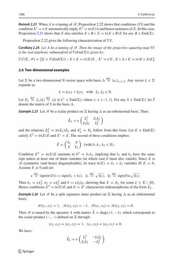
2.6 Two-dimensional examples
Let � be a two-dimensional R-vector space with basis �def.= {ei }i=1,2. Any vector ξ ∈ �
expands as:
ξ = ξ1e1 + ξ2e2 with ξ1, ξ2 ∈ R.
Let Eξdef.= Eκ (ξ)
def.= κξ ⊗ ξ∗ ∈ End(�), where κ ∈ {−1, 1}. For any S ∈ End(�), let Sdenote the matrix of S in the basis �.
Example 2.25 Let B be a scalar product on � having � as an orthonormal basis. Then:
Eξ = κ
(ξ21 ξ1ξ2ξ1ξ2 ξ22
)
and the relations E2ξ = tr(Eξ )Eξ and Et
ξ = Eξ follow from this form. Let E ∈ End(�)
satisfy E2 = tr(E)E and Et = E . The second of these conditions implies:
E =(k1 bb k2
)(with b, k1, k2 ∈ R).
Condition E2 = tr(E)E amounts to b2 = k1k2, implying that k1 and k2 have the samesign unless at least one of them vanishes (in which case b must also vanish). Since E isB -symmetric (and hence diagonalizable), its trace tr(E) = k1 + k2 vanishes iff E = 0.Assume E �= 0 and set:
κdef.= sign(tr(E)) = sign(k1 + k2), ξ1
def.= √|k1|, ξ2def.= sign(b)κ
√|k2|.Then k1 = κξ21 , k2 = κξ22 and b = κξ1ξ2, showing that E = Eξ for some ξ ∈ � \ {0}.Hence conditions E2 = tr(E)E and E = Et characterize endomorphisms of the form Eξ .
Example 2.26 Let B be a split signature inner product on � having � as an orthonormalbasis:
B (e1, e1) = 1, B (e2, e2) = −1, B (e1, e2) = B (e2, e1) = 0.
Then B is tamed by the operator A with matrix A = diag(+1,−1), which corresponds tothe scalar product (−,−) defined on � through:
(e1, e1) = (e2, e2) = 1, (e1, e2) = (e2, e1) = 0.
We have:
Eξ = κ
(ξ21 −ξ1ξ2ξ1ξ2 −ξ22
)
123
Spinors of real type as polyforms and the generalized Killing equation 1367
and the relations E2ξ = tr(Eξ )Eξ and Et
ξ = Eξ follow directly from this form, where t
denotes the adjoint taken with respect to B . Let E ∈ End(�) satisfy Et = E . Then:
E =(k1 −bb k2
)and E A =
(k1 bb −k2
)(with b, k1, k2 ∈ R).
Direct computation shows that the conditions E2 = tr(E)E and E ◦ A ◦ E = tr(E ◦ A)Eare equivalent to each other in this two-dimensional example and amount to the relationb2 = −k1k2, which implies that E vanishes iff k1 = k2. Let us assume that E �= 0 and set:
κdef.= tr(E ◦ A) = sign(k1 − k2), ξ1
def.= √|k1|, ξ2def.= sign(b)κ
√|k2|,where sign(b)
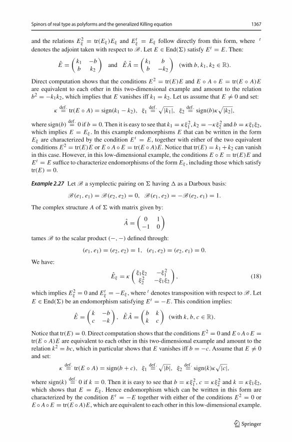
def.= 0 if b = 0. Then it is easy to see that k1 = κξ21 , k2 = −κξ22 and b = κξ1ξ2,which implies E = Eξ . In this example endomorphisms E that can be written in the formEξ are characterized by the condition Et = E , together with either of the two equivalentconditions E2 = tr(E)E or E ◦ A ◦ E = tr(E ◦ A)E . Notice that tr(E) = k1+ k2 can vanishin this case. However, in this low-dimensional example, the conditions E ◦ E = tr(E)E andEt = E suffice to characterize endomorphisms of the form Eξ , including those which satisfytr(E) = 0.
Example 2.27 Let B a symplectic pairing on � having � as a Darboux basis:
B (e1, e1) = B (e2, e2) = 0, B (e1, e2) = −B (e2, e1) = 1.
The complex structure A of � with matrix given by:
A =(
0 1−1 0
)
tames B to the scalar product (−,−) defined through:(e1, e1) = (e2, e2) = 1, (e1, e2) = (e2, e1) = 0.
We have:
Eξ = κ
(ξ1ξ2 −ξ21ξ22 −ξ1ξ2
), (18)
which implies E2ξ = 0 and Et
ξ = −Eξ , where t denotes transposition with respect toB . LetE ∈ End(�) be an endomorphism satisfying Et = −E . This condition implies:
E =(k −bc −k
), E A =
(b kk c
)(with k, b, c ∈ R).
Notice that tr(E) = 0. Direct computation shows that the conditions E2 = 0 and E ◦ A◦E =tr(E ◦ A)E are equivalent to each other in this two-dimensional example and amount to therelation k2 = bc, which in particular shows that E vanishes iff b = −c. Assume that E �= 0and set:
κdef.= tr(E ◦ A) = sign(b + c), ξ1
def.= √|b|, ξ2def.= sign(k)κ
√|c|,where sign(k)
def.= 0 if k = 0. Then it is easy to see that b = κξ21 , c = κξ22 and k = κξ1ξ2,which shows that E = Eξ . Hence endomorphism which can be written in this form arecharacterized by the condition Et = −E together with either of the conditions E2 = 0 orE ◦ A◦E = tr(E ◦ A)E , which are equivalent to each other in this low-dimensional example.
123
1368 V. Cortés et al.
2.7 Including linear constraints
The following result will be used in Sects. 3 and 4.
Proposition 2.28 Let Q ∈ End(�) and κ ∈ {−1, 1} be a fixed sign factor. A real spinorξ ∈ � satisfies Q(ξ) = 0 if and only if Q ◦ Eκ (ξ) = 0 or, equivalently, Eκ (ξ) ◦ Qt = 0,where Qt is the adjoint of Q with respect to B .
Proof Take ξ ∈ � and assume Q(ξ) = 0. Then:
(Q ◦ Eκ (ξ))(χ) = κ Q(ξ) ξ∗(χ) = 0 ∀χ ∈ �
and hence Q ◦ Eκ (ξ) = 0. Conversely, assume that Q ◦ Eκ (ξ) = 0 and pick χ ∈ � suchthat ξ∗(χ) �= 0 (which is possible sinceB is non-degenerate). Then the same calculation asbefore gives:
Q(ξ) ξ∗(χ) = 0,
implying Q(ξ) = 0. The statement for Qt follows from the fact that B -transposition is ananti-automorphism of the R-algebra (End(�), ◦), upon noticing that the relation Eκ (ξ)t =σEκ (ξ) implies (Q ◦ Eκ (ξ))t = σEκ (ξ) ◦ Qt . ��Example 2.29 Let (�,B ) be a two-dimensional Euclidean vector space with orthonormalbasis � as in Example 2.25. Let Q ∈ End(�) have matrix:
Q =(q 00 0
)(with q ∈ R
×)
in this basis. Given ξ ∈ �, Example 2.25 gives:
Eξ = κ
(ξ21 ξ1ξ2ξ1ξ2 ξ22
), Q Eξ = κ
(ξ21 q qξ1ξ20 0
).
Thus Q ◦ Eξ vanishes iff ξ1 = 0, i.e. iff Q(ξ) = 0.
3 From real spinors to polyforms
3.1 Admissible pairings for irreducible real Cliffordmodules
Let V be an oriented d-dimensional R-vector space equipped with a non-degenerate metrich of signature p− q ≡8 0, 2 (hence the dimension d = p+ q of V is even) and let (V ∗, h∗)be the quadratic space dual to (V , h), where h∗ denotes the metric dual to h. Let Cl(V ∗, h∗)be the real Clifford algebra of this dual quadratic space, viewed as a Z2-graded associativealgebra with decomposition:
Cl(V ∗, h∗) = Clev(V ∗, h∗)⊕ Clodd(V ∗, h∗).
In our conventions, the Clifford algebra satisfies (notice the sign !):
θ2 = +h∗(θ, θ) ∀θ ∈ V ∗. (19)
Let π denote the standard automorphism of Cl(V ∗, h∗), which acts as minus the identity onV ∗ ⊂ Cl(V ∗, h∗) and τ denote the standard anti-automorphism, which acts as the identityon V ∗ ⊂ Cl(V ∗, h∗). These two commute and their composition is an anti-automorphism
123
Spinors of real type as polyforms and the generalized Killing equation 1369
denoted by τ = π ◦ τ = τ ◦ π . Let Cl×(V ∗, h∗) denote the group of units Cl(V ∗, h∗).Its twisted adjoint action is the morphism of groups Ad : Cl×(V ∗, h∗)→ Aut(Cl(V ∗, h∗))defined through:
Adx (y) = π(x) y x−1 ∀ x, y ∈ Cl×(V ∗, h∗).
We denote byL(V ∗, h∗) ⊂ Cl(V ∗, h∗) the Clifford group, which is defined as follows:
L(V ∗, h∗) def.= {
x ∈ Cl×(V ∗, h∗) | Adx (V ∗) = V ∗},
This fits into the short exact sequence:
1→ R× ↪→ L
(V ∗, h∗) Ad−→ O(V ∗, h∗)→ 1, (20)
where O(V ∗, h∗) is the orthogonal group of the quadratic space (V ∗, h∗). Recall that the pinand spin groups of (V ∗, h∗) are the subgroups of L
(V ∗, h∗) defined through:
Pin(V ∗, h∗) def.= {x ∈ L
(V ∗, h∗) | N (x)2 = 1},
Spin(V ∗, h∗) def.= Pin(V ∗, h∗) ∩ Clev(V ∗, h∗),
where N : L(V ∗, h∗)→ R× is the Clifford norm morphism, which is given by:
N (x)def.= τ (x) x ∀x ∈ L
(V ∗, h∗).
We have N (x)2 = N (π(x))2 for all x ∈ L(V ∗, h∗). For pq �= 0, the groups SO(V ∗, h∗),
Spin(V ∗, h∗) and Pin(V ∗, h∗) are disconnected; the first have two connected componentswhile the last has four. The connected components of the identity in Spin(V ∗, h∗) andPin(V ∗, h∗) coincide, being given by:
Spin0(V∗, h∗) = {
x ∈ L(V ∗, h∗) | N (x) = 1
}andwe have Spin(V ∗, h∗)/Spin0(V ∗, h∗) � Z2 and Pin(V ∗, h∗)/Spin0(V ∗, h∗) � Z2×Z2.
Let � be a finite-dimensional R-vector space and γ : Cl(V ∗, h∗) → End(�) a Cliffordrepresentation. Then Spin(V ∗, h∗) acts on � through the restriction of γ and (20) inducesthe short exact sequence:
1→ Z2 → Spin(V ∗, h∗) Ad−→ SO(V ∗, h∗)→ 1, (21)
which in turn gives the exact sequence:
1→ Z2 → Spin0(V∗, h∗) Ad−→ SO0(V
∗, h∗)→ 1.
Here SO0(V ∗, h∗) denotes the connected component of the identity of the special orthogonalgroup SO(V ∗, h∗). In signatures p − q ≡8 0, 2 (the “real/normal simple case” of [70]),the algebra Cl(V ∗, h∗) is simple and isomorphic (as a unital associative R-algebra) to the
algebra of square realmatrices of size N = 2d2 . In such signatures Cl(V ∗, h∗) admits a unique
irreducible real left module �, which has dimension N . This irreducible representation is
faithful and surjective, hence in such signatures the representation map γ : Cl(V ∗, h∗) �−→End(�) is an isomorphism of unital R-algebras.
We will equip� with a non-degenerate bilinear pairing which is compatiblewith Cliffordmultiplication. Ideally, such compatibility should translate into invariance under the naturalaction of the pin group. However, this condition cannot be satisfied when if pq �= 0. Instead,we consider the weaker notion of admissible bilinear pairing introduced in [4,5] (see [63,66,
123
1370 V. Cortés et al.
70] for applications to supergravity), which encodes the best compatibility condition withClifford multiplication that can be imposed on a bilinear pairing on� in arbitrary dimensionand signature. The following result of [56] summarizes the main properties of admissiblebilinear pairings.
Theorem 3.1 [56, Theorem 13.17] Suppose that h has signature p − q ≡8 0, 2. Then theirreducible real Clifford module � admits two non-degenerate bilinear pairings B+ : � ×� → R and B− : � × � → R (each determined up to multiplication by a non-zero realnumber) such that:
B+(γ (x)(ξ1), ξ2) = B+(ξ1, γ (τ (x))(ξ2)),B−(γ (x)(ξ1), ξ2) = B−(ξ1, γ (τ (x))(ξ2)), (22)
for all x ∈ Cl(V ∗, h∗) and ξ1, ξ2 ∈ �. The symmetry properties of B+ and B− are as
follows in terms of the modulo 4 reduction of kdef.= d
2 :
k mod 4 0 1 2 3
B+ Symmetric Symmetric Skew-symmetric Skew-symmetricB− Symmetric Skew-symmetric Skew-symmetric Symmetric
In addition, if B s (with s ∈ {−1, 1}) is symmetric, then it is of split signature unlesspq = 0, in which case B s is definite.
Definition 3.2 The sign factor s appearing in the previous theorem is called the adjoint typeof B s , hence B+ is of positive adjoint type (s = +1) and B− is of negative adjoint type(s = −1).
Relations (22) can be written as:
γ (x)t = γ ((π1−s2 ◦ τ)(x)) ∀x ∈ Cl(V ∗, h∗), (23)
where t denotes the B s-adjoint. The symmetry type of an admissible bilinear form B willbe denoted by σ ∈ {−1, 1}. If σ = +1 then B is symmetric whereas if σ = −1 then B isskew-symmetric. Notice that σ depends both on s and on the mod 4 reduction of d
2 .
Definition 3.3 A (real) paired simpleCliffordmodule for (V ∗, h∗) is a triplet� = (�, γ,B ),where (�, γ ) is a simple Cl(V ∗, h∗)-module andB is an admissible pairing on (�, γ ). Wesay that � has adjoint type s ∈ {−1, 1} and symmetry type σ {−1, 1} if B has these adjointand symmetry types.
Remark 3.4 Admissible bilinear pairings of positive and negative adjoint types are relatedthrough the pseudo-Riemannian volume form ν of (V ∗, h∗):
B+ = C B− ◦ (γ (ν)⊗ Id), (24)
for an appropriate non-zero real constantC . For specific applications, we will choose to workwith B+ or with B− depending on which admissible pairing yields the computationallysimplest polyform associated to a given spinor ξ ∈ �. When pq = 0, we will take B s tobe positive-definite (which we can always achieve by rescaling it with a non-zero constantof appropriate sign). See [70] for a useful discussion of properties of admissible pairings invarious dimensions and signatures.
123
Spinors of real type as polyforms and the generalized Killing equation 1371
Remark 3.5 Directly from their definition, the pairings B s satisfy:
B s(γ (π1+s2 (x))(ξ1), γ (x)(ξ2)) = N (x)B s(ξ1, ξ2) ∀ x ∈ Cl(V ∗, h∗) ∀ ξ1, ξ2 ∈ �.
This relation yields:
B s(γ (x)(ξ1), ξ2)+B s(ξ1, γ (x)(ξ2)) = 0 ∀ ξ1, ξ2 ∈ �
for all x = θ1 · θ2 with h∗-orthogonal θ1, θ2 ∈ V ∗. This implies that B s is invariant underthe action of Spin(V ∗, h∗) and hence also under Spin0(V ∗, h∗). If h is positive-definite, thenB+ is Pin(V ∗, h∗)-invariant, since it satisfies:
B+(γ (θ)(ξ1), γ (θ)(ξ2)) = B+(ξ1, ξ2) ∀ξ1, ξ2 ∈ �
for all θ ∈ V ∗ of unit norm. If h is negative-definite, then B− is Pin(V ∗, h∗)-invariant.
For completeness, let us give an explicit construction of B+ and B−. Pick an h∗-orthonormal basis
{ei
}i=1,...,d of V ∗ and let:
K({ei
})def.= {1} ∪
{±ei1 · · · · · eik | 1 ≤ i1 < · · · < ik ≤ d , 1 ≤ k ≤ d
}
be the finite multiplicative subgroup of Cl(V ∗, h∗) generated by the elements±ei . Averagingover K(
{ei
}), we construct an auxiliary positive-definite inner product (−,−) on � which
is invariant under the action of this group. This product satisfies:
(γ (x)(ξ1), γ (x)(ξ2)) = (ξ1, ξ2) ∀x ∈ K({ei }) ∀ ξ1, ξ2 ∈ �.
Write V ∗ = V ∗+ ⊕ V ∗−, where V ∗+ is a p-dimensional subspace of V ∗ on which h∗ is positivedefinite and V ∗− is a q-dimensional subspace of V ∗ on which h∗ is negative-definite. Fix anorientation on V ∗+ (which induces a unique orientation on V ∗− compatible with the orientationofV ∗ induced from that ofV ) anddenote by ν+ and ν− the correspondingpseudo-Riemannianvolume forms. We have ν = ν+ ∧ ν−. For p (and hence q) odd, define:
B±(ξ1, ξ2) = (γ (ν±)(ξ1), ξ2) ∀ξ1, ξ2 ∈ �, (25)
whereas for p (and hence q) even, set:
B±(ξ1, ξ2) = (γ (ν∓)(ξ1), ξ2) ∀ξ1, ξ2 ∈ �. (26)
Then B± are admissible pairings in the sense of Theorem 3.1. Direct computation usingEqs. (25) and (26) gives the following result, which fixes the constant C appearing inRemark 3.4.
Proposition 3.6 The admissible pairings B+ and B− constructed above are related asfollows:
B+ = (−1)[ q2 ]B−(γ (ν)⊗ Id). (27)
Thus we can normalize B± such that the constant in (24) is given by C = (−1)[ q2 ].Proposition 3.7 Let B be an admissible pairing on the real simple Cl(V ∗, h∗)-module(�, γ ). Then B is invariant under the action of the group Spin0(V
∗, h∗) on � obtainedby restricting γ .
123
1372 V. Cortés et al.
Proof We have to show the relation:
γ (x)t ◦ γ (x) = Id ∀x ∈ Spin0(V∗, h∗). (28)
Consider orthonormal basis {ei }i=1,...,d of (V ∗, h∗) such that h∗(ei , ei ) = +1 for i =1, . . . , p and h∗(ei , ei ) = −1 for i = p+1, . . . , d . A simple computation using relation (23)shows that (28) holds for x of the form ei1 ·· · ··ei2k ·e j1 ·· · ··e j2l , where 1 ≤ i1 ≤ · · · ≤ i2k ≤ pand p + 1 ≤ j1 ≤ · · · ≤ j2l ≤ d with 0 ≤ 2k ≤ p and 0 ≤ 2l ≤ q . Since such elementsgenerate Spin0(V
∗, h∗), we conclude. ��
3.2 The Kähler–Atiyahmodel ofCl(V∗, h∗)
To identify spinors with polyforms, we will use an explicit realization of Cl(V ∗, h∗) as adeformation of the exterior ∧V ∗. This model (which goes back to the work of Chevalley andRiesz [20,21,83]) has an interpretation as a deformation quantization of the odd symplecticvector space obtained by parity change from the quadratic space (V , h) (see [12,86]). It canbe constructed using the symbol map and its inverse, the quantization map. Consider first thelinear map f : V ∗ → End(∧V ∗) given by:
f(θ)(α) = θ ∧ α + ιθ�α ∀θ ∈ V ∗ ∀α ∈ ∧V ∗.We have:
f(θ) ◦ f(θ) = h∗(θ, θ) ∀θ ∈ V ∗.
By the universal property ofClifford algebras, it follows that f extends uniquely to amorphismf : Cl(V ∗, h∗)→ End(∧V ∗) of unital associative algebras such that f◦i = f, where i : V ∗ ↪→Cl(V ∗, h∗) is the canonical inclusion of V in Cl(V ∗, h∗).
Definition 3.8 The symbol (orChevalley–Riesz)map is the linearmap l : Cl(V ∗, h∗)→ ∧V ∗defined through:
l(x) = f(x)(1) ∀x ∈ Cl(V ∗, h∗),
where 1 ∈ R is viewed as an element of ∧0(V ∗) = R.
The symbol map is an isomorphism of filtered vector spaces. We have:
l(1) = 1, l(θ) = θ, l(θ1 · θ2) = θ1 ∧ θ2 + h∗(θ1, θ2) ∀θ, θ1, θ2 ∈ V ∗.
As expected, l is not a morphism of algebras. The inverse:
�def.= l−1 : ∧ V ∗ → Cl(V ∗, h∗).
of l (called the quantization map) allows one to view Cl(V ∗, h∗) as a deformation of theexterior algebra (∧V ∗,∧) (see [12,86]). Using l and �, we transport the algebra product ofCl(V ∗, h∗) to an h-dependent unital associative product defined on ∧V ∗, which deforms thewedge product.
Definition 3.9 The geometric product � : ∧V ∗ × ∧V ∗ → ∧V ∗ is defined through:α1 � α2 def.= l(�(α1) ·�(α2)) ∀α1, α2 ∈ ∧V ∗,
where · denotes multiplication in Cl(V ∗, h∗).
123
Spinors of real type as polyforms and the generalized Killing equation 1373
By definition, the map � is an isomorphism of unital associative R-algebras3 from(∧V ∗,�) to Cl(V ∗, h∗). Through this isomorphism, the inclusion V ∗ ↪→ Cl(V ∗, h∗) corre-sponds to the natural inclusion V ∗ ↪→ ∧V ∗. We shall refer to (∧V ∗,�) as theKähler–Atiyahalgebra of the quadratic space (V , h) (see [47,61]). It is easy to see that the geometric productsatisfies:
θ � α = θ ∧ α + ιθ�α ∀θ ∈ V ∗ ∀α ∈ ∧V ∗.Also notice the relation:
θ � θ = h∗(θ, θ) ∀θ ∈ V ∗.
The maps π and τ transfer through� to the Kähler–Atiyah algebra, producing unital (anti)-automorphisms of the latter which we denote by the same symbols. With this notation, wehave:
π ◦� = � ◦ π, τ ◦� = � ◦ τ. (29)
For any orthonormal basis {ei }i=1,...,d of V ∗ and any k ∈ {1, . . . , d}, we have e1 � · · · � ek =e1 ∧ · · · ∧ ek and:
π(e1 ∧ · · · ∧ ek) = (−1)ke1 ∧ · · · ∧ ek, τ (e1 ∧ · · · ∧ ek) = ek ∧ · · · ∧ e1.
Let T (V ∗) denote the tensor algebra of the (parity change of) V ∗, viewed as a Z-gradedassociative superalgebra whose Z2-grading is the reduction of the natural Z-grading; thuselements of V have integer degree one and they are odd. Let:
Der(T (V ∗)) def.=⊕k∈Z
Derk(T (V ∗))
denote the Z-graded Lie superalgebra of all superderivations. The minus one integer degreecomponent Der−1(T (V ∗)) is linearly isomorphic with the space Hom(V ∗,R) = V actingby contractions:
ιv(θ1 ⊗ · · · ⊗ θk) =k∑
i=1(−1)i−1θ1 ⊗ · · · ⊗ ιvθi ⊗ · · · ⊗ θk ∀v ∈ V ∀θ1, . . . , θk ∈ V ∗,
while the zero integer degree component Der0(T (V ∗)) = End(V ∗) = gl(V ∗) acts through:
L A(θ1 ⊗ · · · ⊗ θk) =k∑
i=1θ1 ⊗ · · · ⊗ A(θi )⊗ · · · ⊗ θk ∀A ∈ gl(V ∗).
We have an isomorphism of super-Lie algebras:
Der−1(T (V ∗))⊕ Der0(T (V ∗)) � V � gl(V ∗).
The action of this super Lie algebra preserves the ideal used to define the exterior algebraas a quotient of T (V ∗) and hence descends to a morphism of super Lie algebras L� : V �
gl(V ∗) → Der(∧V ∗,∧). Contractions also preserve the ideal used to define the Clifford
3 Notice that the geometric product is not compatible with the grading of ∧V ∗ given by form rank, but onlywith its mod 2 reduction, because the quantization map does not preserve Z-gradings. Hence the Kähler–Atiyah algebra is not isomorphic with Cl(V ∗, h∗) in the category of Clifford algebras defined in [69]. Assuch, it provides a different viewpoint on spin geometry, which is particularly useful for our purpose (see[63,66,70,71]).
123
1374 V. Cortés et al.
algebra as a quotient of T (V ∗). On the other hand, endomorphisms A of V ∗ preserve thatideal iff A ∈ so(V ∗, h∗). Together with contractions, they induce a morphism of super Liealgebras LCl : V � so(V ∗, h∗)→ Der(Cl(V ∗, h∗)). The following result states that L� andLCl are compatible with l and �.
Proposition 3.10 [75, Proposition 2.11] The quantization and symbol maps intertwine theactions of V � so(V ∗, h∗) on Cl(V ∗, h∗) and ∧V ∗:
�(L�(ϕ)(α)) = LCl(ϕ)(�(α)), l(LCl(ϕ)(x)) = L�(ϕ)(l(x)),
for all ϕ ∈ V � so(V ∗, h∗), α ∈ ∧V ∗ and x ∈ Cl(V ∗, h∗).
This proposition shows that quantization is equivariant with respect to affine orthogonaltransformations of (V ∗, h∗). In signatures p− q ≡8 0, 2, composing � with the irreduciblerepresentation γ : Cl(V ∗, h∗)→ End(�) (which in such signatures is a unital isomorphismof algebras) gives an isomorphism of unital associative R-algebras4:
�γdef.= γ ◦� : (∧V ∗,�) ∼→ (End(�), ◦). (30)
Since�γ is an isomorphismof algebras and (∧V ∗,�) is generated byV ∗, the identity togetherwith the elements �γ (ei1 ∧ · · · ∧ eik ) = γ (ei1) ◦ · · · ◦ γ (eik ) for 1 ≤ i1 < · · · < ik ≤ d andk = 1, . . . , d form a basis of End(�).
Remark 3.11 We sometimes denote the action of a polyform α ∈ ∧V ∗ as an endomorphismon � by a dot (this corresponds to Clifford multiplication through the isomorphism �γ ):
α · ξ def.= �γ (α)(ξ) ∀α ∈ ∧V ∗ ∀ξ ∈ �.
The trace on End(�) transfers to the Kähler–Atiyah algebra through the map �γ (see[70]):
Definition 3.12 The Kähler–Atiyah trace is the linear functional:
S : ∧ V ∗ → R, α �→ tr(�γ (α)).
Wewill see in a moment that S does not depend on γ or h. Since�γ is a unital morphismof algebras, we have:
S(1) = dim(�) = N = 2d2 and S(α1 � α2) = S(α2 � α1) ∀α1, α2 ∈ ∧V ∗,
where 1 ∈ R = ∧0V ∗ is the unit element of the field R of real numbers.
Lemma 3.13 For any 0 < k ≤ d, we have:
S|∧k V ∗ = 0.
Proof Let{ei
}i=1,...,d be an orthonormal basis of (V ∗, h∗). For i �= j we have ei � e j =
−e j � ei and hence (ei )−1 � e j � ei = −e j . Let 0 < k ≤ d and 1 ≤ i1 < · · · < ik ≤ d . If kis even, then:
S(ei1 � · · · � eik ) = S(eik � ei1 � · · · � eik−1) = (−1)k−1S(ei1 � · · · � eik ),4 This isomorphism identifies the deformation quantization (∧V ∗, �) of the exterior algebra (∧V ∗,∧) withthe operator quantization (End(�), ◦) of the latter.
123
Spinors of real type as polyforms and the generalized Killing equation 1375
and hence S(ei1 � · · · � eik ) = 0. Here we used cyclicity of the Kähler–Atiyah trace and thefact that eik anticommutes with ei1 , . . . , eik−1 . If k is odd, let j ∈ {1, . . . , d} be such thatj /∈ {i1, . . . , ik} (such a j exists since k < d). We have:
S(ei1 � · · · � eik ) = S((e j )−1 � ei1 � · · · � eik � e j ) = −S(ei1 � · · · � eik ) = 0
and we conclude. ��Let α(k) ∈ ∧kV ∗ denote the degree k component of α ∈ ∧V ∗. Lemma 3.13 implies:
Proposition 3.14 The Kähler–Atiyah trace is given by:
S(α) = dim(�) α(0) = 2d2 α(0) ∀α ∈ ∧V ∗.
In particular, S does not depend on the irreducible representation γ of Cl(V ∗, h∗) or on h.
Lemma 3.15 Let α ∈ ∧V ∗ and B be an admissible bilinear pairing of (�, γ ) of adjointtype s ∈ {−1, 1}. Then the following equation holds:
�γ (α)t = �γ (α
t ), (31)
where �γ (α)t is the B -adjoint of �γ (α) and we defined the s-transpose of α through:
αt def.= (π1−s2 ◦ τ)(α).
Proof Follows immediately from (23) and relations (29). ��
3.3 Spinor squaringmaps
Definition 3.16 Let � = (�, γ,B ) be a paired simple Clifford module for (V ∗, h∗). Thesigned spinor squaring maps of � are the quadratic maps:
E±�def.= �−1γ ◦ E± : �→ ∧V ∗,
where E± : � → End(�) are the signed squaring maps of the paired vector space (�,B )
which were defined in Sect. 2. Given a spinor ξ ∈ �, the polyforms E+� (ξ) and E−� (ξ) =−E+� (ξ) are called the positive and negative squares of ξ relative to the admissible pairingB . A polyform α ∈ ∧V ∗ is called a signed square of ξ ∈ � if α = E+� (ξ) or α = E−� (ξ).
Consider the following subsets of ∧V ∗:Z := Z(�)
def.= �−1γ (Z(�,B )), Z± := Z±(�)def.= �−1γ (Z±(�,B )).
Since �γ is a linear isomorphism, Sect. 2 implies that E±� are two-to-one except at 0 ∈ �
and:
Z− = −Z+, Z+ ∩ Z− = {0}, Z = Z+ ∪ Z−.
Moreover, E±� induce the same bijective map:
E� : �/Z2∼→ Z(�)/Z2. (32)
Notice that Z is a cone in ∧V ∗, which is the union of the opposite half cones Z±.
Definition 3.17 The bijection (32) is called the class spinor squaringmap of the paired simpleClifford module � = (�, γ,B ).
123
1376 V. Cortés et al.
We will sometimes denote by αξdef.= E+� (ξ) ∈ Z+(�) the positive polyform square of
ξ ∈ �.
Remark 3.18 The representationmap γ is an isomorphismwhen p−q ≡8 0, 2. This does nothold in other signatures, for which the construction of spinor squaring maps is more delicate(see [70]).
The following result is a direct consequence of Proposition 3.10.
Proposition 3.19 The quadratic maps E±� : �→ ∧V ∗ are Spin0(V ∗, h∗)-equivariant:E±� (u ξ) = Adu(E±� (ξ)) ∀u ∈ Spin0(V
∗, h∗) ∀ξ ∈ �,
where the right hand side denotes the natural action of Adu ∈ O(V ∗, h∗) on ∧V ∗.We are ready to give the algebraic characterization of spinors in terms of polyforms.
Theorem 3.20 Let � = (�, γ,B ) be a paired simple Clifford module for (V ∗, h∗) of sym-metry type σ and adjoint type s. Then the following statements are equivalent for a polyformα ∈ ∧V ∗:(a) α is a signed square of some spinor ξ ∈ �, i.e. it lies in the set Z(�).(b) α satisfies the following relations:
α � α = S(α) α, (π1−s2 ◦ τ)(α) = σ α, α � β � α = S(α � β) α (33)
for a fixed polyform β ∈ ∧V ∗ which satisfies S(α � β) �= 0.(c) The following relations hold:
(π1−s2 ◦ τ)(α) = σ α, α � β � α = S(α � β) α (34)
for any polyform β ∈ ∧V ∗.In particular, the set Z(�) depends only on σ , s and (V ∗, h∗).
In view of this result, we will also denote Z(�) by Zσ,s(V ∗, h∗).
Proof Since � : Cl(V ∗, h∗) → End(�) is a unital isomorphism algebras, α satisfies (34)iff:
Et = σ E, E ◦ A ◦ E = tr(E ◦ A)E ∀ A ∈ End(�), (35)
where Edef.= �−1γ (α), A
def.= �−1γ (β) and we used Lemma 3.15 and the definition andproperties of the Kähler-Atiyah trace. The conclusion now follows from Proposition 2.21. ��
The second equation in (34) implies:
Corollary 3.21 Let α ∈ Zσ,s(V ∗, h∗). If k ∈ {1, . . . , d} satisfies:(−1)k 1−s
2 (−1) k(k−1)2 = −σ,
then α(k) = 0.
Polyform α ∈ Z±(�) admits an explicit presentation which first appeared in [63,66,70].
123
Spinors of real type as polyforms and the generalized Killing equation 1377
Proposition 3.22 Let{ei
}i=1,...,d be an orthonormal basis of (V ∗, h∗) and κ ∈ {−1, 1}.
Then every polyform α ∈ Zκ (�) can be written as:
α = κ
2d2
d∑k=0
∑i1<···<ik
B ((γ (eik )−1 ◦ · · · ◦ γ (ei1)−1)(ξ), ξ) ei1 ∧ · · · ∧ eik , (36)
where the spinor ξ ∈ � is determined by α up to sign.
Remark 3.23 We have:
γ (ei )−1 = h∗(ei , ei )γ (ei ) = h(ei , ei )γ (ei ),
where {ei }i=1,...,d is the contragradient orthonormal basis of (V , h). For simplicity, set:
γ i def.= γ (ei ) and γidef.= h(ei , ei )γ (e
i ),
so that (γ i )−1 = γi . Then the degree one component in (36) reads:
α(1) = κ
2d2
B (γi (ξ), ξ)ei
and its dual vector field (α(1))� = κ
2d2B (γi (ξ), ξ)ei is called the (signed) Dirac vector of
ξ relative to B . For spinors on a manifold (see Sect. 4), this vector globalizes to the Diraccurrent.
Proof It is easy to see that the set:
Pdef.= {Id} ∪
{γ 1 ◦ · · · ◦ γ i1 ◦ · · · γ ik ◦ · · · ◦ γ d | 1 ≤ i1 < · · · < ik ≤ d, k = 1, . . . , d
},
gives an orthogonal basis of End(�)with respect to the nondegenerate and symmetric bilinearpairing induced by the trace:
End(�)× End(�)→ R, (A1, A2) �→ tr(A1A2).
In particular, the endomorphism Edef.= �γ (α) ∈ Zκ (�) expands as:
E = 1
2d2
d∑k=0
∑i1<···<ik
tr((γ i1 ◦ · · · ◦ γ ik )−1 ◦ E) γ i1 ◦ · · · ◦ γ ik
= κ
2d2
d∑k=0
∑i1<···<ik
B ((γ i1 ◦ · · · ◦ γ ik )−1(ξ), ξ) γ i1 ◦ · · · ◦ γ ik ,
where ξ ∈ � is a spinor such that E = Eκ (ξ) andwe noticed that tr(B◦Eκ (ξ)) = κ tr(B(ξ)⊗ξ∗) = κ ξ∗(B(ξ)) = κ B (Bξ, ξ) for all B ∈ End(�). The conclusion follows by applyingthe isomorphism algebras �−1γ : (End(�), ◦)→ (∧V ∗,�) to the previous equation. ��
Lemma 3.24 The following identities hold for all α ∈ ∧V ∗:α � ν = ∗ τ(α), ν � α = ∗ (π ◦ τ)(α). (37)
123
1378 V. Cortés et al.
Proof Since multiplication by ν is R-linear, it suffices to consider homogeneous elementsα = ei1 ∧ · · · ∧ eik with 1 ≤ i1 < · · · < ik ≤ d , where
{ei
}i=1,...,d is an orthonormal basis
of (V ∗, h∗). We have:
ei1 ∧ · · · ∧ eik � ν= ei1 � · · · � eik � e1 � · · · � ed= (−1)i1+···+ik (−1)ke1 � · · · � (ei1)2 � ei1+1 � · · · � (eik )2 � eik+1 � · · · � ed= h∗(ei1 , ei1) · · · h∗(eik , eik ) (−1)i1+···+ik (−1)ke1 � · · · � ei1−1 �ei1+1 · · · � eik−1 � eik+1 � · · · � ed= (−1) k(k−1)
2 (−1)2(i1+···+ik )(−1)2k ∗ (ei1 ∧ · · · ∧ eik ) = ∗τ(α),which implies α � ν = ∗ τ(α). Using the obvious relation α � ν = (ν � π)(α), we conclude.
��
The following shows that the choice of admissible pairing used to construct the spinorsquare map is a matter of taste, see also Remark 3.4.
Proposition 3.25 Let ξ ∈ � and denote by α±ξ ∈ Z+ the positive polyform squares of ξrelative to the admissible pairingsB+ andB− of (�, γ ), which we assume to be normalizedsuch that they are related through (27). Then the following relation holds:
∗α+ξ = (−1)[ q+12 ]+p(q+1)(−1)dc(α−ξ ).
where c : ∧ V ∗ → ∧V ∗ is the linear map which acts as multiplication by k!(d−k)! in each
degree k.
Proof We compute:
∗(α+ξ )(k) = 1
2d2
B+((γik ◦ · · · ◦ γi1)(ξ), ξ) ∗ (ei1 ∧ · · · ∧ eik )
= (−1)[ q+12 ]+pq(−1) k(k−1)2
√|h|2
d2 (d − k)!
B−((γ (ν) ◦ γi1 ◦ · · · ◦ γik )(ξ), ξ)εii1 ...ikak+1...ad eak+1 ∧ · · · ∧ ead
= (−1)[ q+12 ]+pq(−1) k(k−1)2 (−1)k(d−k) k!
2d2 (d − k)!
B−(γ (ν)γ (∗(eak+1 ∧ · · · ∧ ed))(ξ), ξ)eak+1 ∧ · · · ∧ ed
= (−1)[ q+12 ]+pq(−1) k(k−1)2 (−1) (d−k)(d+k+1)
2k!
2d2 (d − k)!
B−((γ (ν)2 ◦ γ ak+1 ◦ · · · ◦ γ ad )(ξ), ξ)eak+1 ∧ · · · ∧ ed
= (−1)[ q+12 ]+p(q+1)(−1)k k!(d − k)! (α
−ξ )(d−k)
= (−1)[ q+12 ]+p(q+1)(−1)d k!(d − k)!π(α
−ξ )(d−k),
where we used the identity ν � α = ∗(π ◦ τ)(α) proved in Lemma 3.24. ��
123
Spinors of real type as polyforms and the generalized Killing equation 1379
3.4 Linear constraints
The following result will be used in Sects. 3 and 4.
Proposition 3.26 A spinor ξ ∈ � lies in the kernel of an endomorphism Q ∈ End(�) iff:
Q � αξ = 0,
where αξdef.= E+� (ξ) is the positive polyform square of ξ and:
Qdef.= �−1γ (Q) ∈ ∧V ∗
is the dequantization of Q.
Remark 3.27 Taking the s-transpose shows that equation Q � αξ = 0 is equivalent to:
αξ � (π 1−s2 ◦ τ)(Q) = 0.
Proof Follows immediately from Proposition 2.28, using the fact that �γ : (∧V ∗,�) →End(�) is an isomorphism of unital associative algebras. ��
3.5 Real chiral spinors
Theorem3.20 canbe refined for chiral spinors of real type,which exist in signature p−q ≡8 0.In this case, the Clifford volume form ν ∈ Cl(V ∗, h∗) squares to 1 and lies in the center ofClev(V ∗, h∗), giving a decomposition as a direct sum of simple associative algebras:
Clev(V ∗, h∗) = Clev+ (V ∗, h∗)⊕ Clev− (V ∗, h∗),
where we defined:
Clev± (V ∗, h∗)def.= 1
2(1± ν)Cl(V ∗, h∗).
We decompose � accordingly:
� = �(+) ⊕�(−), where �(±) def.= 1
2(Id± γ (ν))(�).
The subspaces �(±) ⊂ � are preserved by the restriction of γ to Clev(V ∗, h∗), whichtherefore decomposes as a sum of two irreducible representations:
γ (+) : Clev(V , h)→ End(�(+)) and γ (−) : Clev(V , h)→ End(�(−))
distinguished by the value which they take on the volume form ν ∈ Clev(V ∗, h∗):
γ (+)(ν) = Id, γ (−)(ν) = −Id.A spinor ξ ∈ � is called chiral of chirality μ ∈ {−1, 1} if it belongs to �(μ). Setting
αξdef.= E+� (ξ), Proposition 3.26 shows that this amounts to the condition:
ν � αξ = μαξ .
For any μ ∈ {−1, 1} and κ ∈ {−1, 1}, define:Z (μ)κ := Z (μ)
κ (�)def.= Eκ
�(�(μ)), Z (μ) := Z (μ)(�)def.= Z (μ)
+ (�) ∪ Z (μ)− (�).
123
1380 V. Cortés et al.
We have Z (μ)− (�) = −Z (μ)
+ (�) and Z (μ)+ (�) ∩ Z (μ)
− (�) = {0}. Moreover, Eκ� restrict to
surjections E(μ),κ� : �(μ) → Z (μ)
κ (�) (which are two to one except at the origin). In turn,
the latter induce bijections E(μ)� : �(μ)/Z2
∼→ Z (μ)(�)/Z2. Theorem 3.20, Proposition 3.26and Lemma 3.24 give:
Corollary 3.28 Let � be a paired simple Cl(V ∗, h∗)-module of symmetry type σ and adjointtype s. The following statements are equivalent for α ∈ ∧V ∗, where μ ∈ {−1, 1} is a fixedchirality type:
(a) α lies in the set Z (μ)(�), i.e. it is a signed square of a chiral spinor of chirality μ.(b) The following conditions are satisfied:
(π1−s2 ◦ τ)(α) = σ α, ∗ (π ◦ τ)(α) = μα, α � α = S(α) α,
α � β � α = S(α � β) α (38)
for a fixed polyform β ∈ ∧V ∗ which satisfies S(α � β) �= 0.(c) The following conditions are satisfied:
(π1−s2 ◦ τ)(α) = σα, ∗ (π ◦ τ)(α) = μα, α � β � α = S(α � β) α (39)
for every polyform β ∈ ∧V ∗.In this case, the real chiral spinor of chirality μ which corresponds to α through the eitherof the maps E(μ),+
� or E(μ),−� is unique up to sign and vanishes iff α = 0.
In particular, Z (μ)(�) depends only on σ, s and (V ∗, h∗) and will also be denoted byZ (μ)σ,s (V ∗, h∗).
Corollary 3.29 Let α ∈ Z (+)σ,s (V ∗, h∗) ∪ Z (−)
σ,s (V ∗, h∗). If k ∈ {1, . . . , d} satisfies:
−(−1)k s−12 (−1) k(k−1)
2 = σ,
then we have α(k) = 0 and α(d−k) = 0.
Proof Follows immediately from Corollary 3.21 and the second relation in (38). ��
3.6 Low-dimensional examples
Let us describe Z and Z (μ) for some low-dimensional cases.
3.6.1 Signature (2, 0)
Let (V ∗, h∗) be a two-dimensional R-vector space with a scalar product h∗. Its irreducibleClifford module (�, γ ) is two-dimensional with an admissible pairing B which is a scalarproduct. Theorem 3.20 with β = 1 shows that w ∈ ∧V ∗ is a signed square of ξ ∈ � iff:
α � α = 2 α(0) α, τ (α) = α. (40)
Writing α = α(0) ⊕ α(1) ⊕ α(2), the second of these relations reads:
α(0) + α(1) − α(2) = α(0) + α(1) + α(2).
123
Spinors of real type as polyforms and the generalized Killing equation 1381
This gives α(2) = 0, whence the first equation in (40) becomes (α(0))2 = h∗(α(1), α(1)).Hence α is a signed square of a spinor iff:
α = ±h∗(α(1), α(1))12 ⊕ α(1) with α(1) ∈ V ∗.
Let{ei
}i=1,2 be an orthonormal basis of (V ∗, h∗) and α = E+� (ξ) for some ξ ∈ �. Then:
2 α = B (ξ, ξ)+B (γi (ξ), ξ) ei .
Thus:
4 h∗(α(1), α(1)) = B (ξ, ξ)2
and hence the norm of ξ determines the norm of one-form α(1) ∈ V ∗.
3.6.2 Signature (1, 1)
Let (V ∗, h∗) be a two-dimensional vector space V ∗ equipped with a Lorentzian metrich∗. Its irreducible Clifford module (�, γ ) is two-dimensional with a symmetric admissiblebilinear pairingB of split signature and positive adjoint type (see Theorem 3.1). To guaranteethat α ∈ ∧V ∗ belongs to Z , we should in principle consider the first equation in (34) ofTheorem 3.20 for all β ∈ ∧V ∗. However, V ∗ is two-dimensional and Example 2.26 showsthat it suffice to take β = 1. Thus α belongs to the set Z+,+(V ∗, h∗) iff:
α � α = 2 α(0) α, τ (α) = α. (41)
Writing α = α0⊕ α(1)⊕ α(2), the second condition gives α(2) = 0, while the first conditionbecomes:
(α(0))2 = h∗(α(1), α(1)).
In particular, α(1) is space-like or null. Hence α is a signed square of a spinor iff:
α = ±h∗(α(1), α(1))12 + α(1) (42)
for a one-form α(1) ∈ V ∗. As in the Euclidean case, we have:
2α = B (ξ, ξ)+B (γi (ξ), ξ) ei ,
whence:
4 h∗(α(1), α(1)) = B (ξ, ξ)2.
Thus α(1) is null iffB (ξ, ξ) = 0. In this signature the volume form squares to 1 and we havechiral spinors. Fix μ ∈ {−1, 1}. By Corollary 3.28, α lies in the set Z (μ)
+,+(V ∗, h∗) iff it hasthe form (42) and satisfies the supplementary condition:
∗ (π ◦ τ)(α) = μα.
This amounts to the following system, where νh is the volume form of (V ∗, h∗):
±h∗(α(1), α(1))12 νh − ∗α(1) = ±μ h∗(α(1), α(1))
12 + μα(1).
Thus h∗(α(1), α(1)) = 0 and ∗α(1) = −μα(1). Hence a signed polyform square of a chiralspinor of chirality μ is a null one-form which is anti-self-dual when μ = +1 and self-dualwhen μ = −1. Notice that the nullity condition on α(1) is equivalent with (anti-)selfduality.
123

1382 V. Cortés et al.
3.6.3 Signature (3, 1)
This case is relevant for supergravity applications andwill arise in Sects. 5 and 6. Let (V ∗, h∗)be aMinkowski space of “mostly plus” signature (3, 1). Its irreducibleCliffordmodule (�, γ )
is four-dimensional and both admissible pairings B± are skew-symmetric. We work withthe admissible pairing B = B− of negative adjoint type.
Definition 3.30 A parabolic pair of one-forms is ordered pair (u, l) ∈ V ∗ × V ∗ such thatu �= 0 and:
h∗(u, u) = 0, h∗(l, l) = 1, h∗(u, l) = 0, (43)
i.e. u is nonzero and null, l is spacelike of unit norm and u is orthogonal to l. Two parabolicpairs of one forms (u, l) and (u′, l ′) are called:
• weakly equivalent, if there exist b ∈ R×, c ∈ R and η ∈ {−1, 1} such that:
u′ = bu and l ′ = ηl + cu. (44)
• equivalent (and we write (u, l) ≡ (u′, l ′)) if there exist b ∈ R× and c ∈ R such that:
u′ = bu and l ′ = l + cu. (45)
• strongly equivalent (and we write (u, l) ∼ (u′, l ′)) if there exist ζ ∈ {−1, 1} and c ∈ R
such that:
u′ = ζu and l ′ = l + cu. (46)
LetP(V ∗, h∗) denote the set of parabolic pairs of one-forms. The binary relations definedabove are equivalence relations on this set;moreover, strong equivalence implies equivalence,which in turn implies weak equivalence.
Recall that a 2-plane� in V ∗ is called parabolic (with respect to h∗) if the restriction h∗�of h∗ to� has one-dimensional kernel. This happens iff� is tangent to the light cone of the
Minkowski space (V ∗, h∗) along a null line. This line coincides with Kh(�)def.= ker(h∗�)
and is called the null line of �. If � ⊂ V ∗ is a parabolic 2-plane, then any element of� which does not belong to Kh(�) is spacelike. The two connected components of thecomplement � \ Kh(�) are the spacelike half-planes of �. An orientation of the null lineKh(�) is called a time orientation of�, while an orientation of the quotient line�/Kh(�) iscalled a co-orientation of�. Notice that a co-orientation of� amounts to a choiceH of oneof the spacelike half-spaces of �. A co-oriented parabolic 2-plane in V ∗ is a pair (�,H),where � is a parabolic two-plane in V ∗ andH is a co-orientation of�. The set of spacelikeunit norm elements of � has two connected components, each of which is an affine lineparallel to Kh(�). These two affine lines are related by the inversion of�with respect to theorigin. Notice that a co-orientationH of � amounts to a choice L of one of these two affinelines. Namely, we associate to L that spacelike half-planeHL of� which contains L . Givenu ∈ Kh(�) \ {0}, a unit norm spacelike element l ∈ � is determined up to transformationsof the form l → ζ l + cu, where ζ ∈ {−1, 1} and c ∈ R.
Remark 3.31 Parabolic 2-planes correspond to degenerate complete flags in (V ∗, h∗) (seeAppendix A). Notice that a parabolic 2-plane� determines a short exact sequence of vectorspaces:
0→ K → �→ N → 0
123
Spinors of real type as polyforms and the generalized Killing equation 1383
with K = Kh(�) and N = �/K and induces a scalar product on the quotient line N .Conversely, giving a “parabolic” metric on a 2-plane � amounts to giving a short exactsequence of this form together with a scalar product on N . A time orientation of � isorientation of K while a co-orientation is an orientation of N . Since the determinant lineof � is given by det(�) = ∧2� = K ⊗ L , a time orientation and a co-orientation takentogether determine an orientation of �.
A basis of a parabolic 2-plane � ⊂ V ∗ is called parabolic if its two elements form aparabolic pair. By Sylvester’s theorem, any parabolic plane � admits parabolic bases.
Proposition 3.32 The map (u, l)→ SpanR(u, l) induces a bijection between the set of weakequivalence classes of parabolic pairs of one-forms and the set of all parabolic 2-planes in(V ∗, h∗).
Proof If (u, v) is a parabolic pair, then SpanR(u, v) is a parabolic 2-plane, which dependsonly on the weak equivalence class of (u, v). Conversely, it is easy to see that any twoparabolic bases of a parabolic 2-plane � in V ∗ are weakly-equivalent as parabolic pairs. ��
Proposition 3.32 implies:
Corollary 3.33 The map (u, l) → (SpanR(u, l),Hl) induces a bijection between the setP(V ∗, h∗)/≡ of equivalence classes of parabolic pairs of one-forms and the set of all co-oriented parabolic 2-planes in (V ∗, h∗), where Hl is the unique spacelike half-plane of theparabolic 2-plane SpanR(u, l) which contains the vector l.
Theorem 3.34 A polyform α ∈ ∧V ∗ is a signed square of a nonzero spinor (i.e. it belongsto the set Z−,−(V ∗, h∗)) iff it has the form:
α = u + u ∧ l (47)
for a parabolic pair of one-forms (u, l) ∈ P(V ∗, h∗). In this case, u is uniquely determinedby α while l is determined by α up to transformations of the form:
l → l + cu, (48)
where c ∈ R is arbitrary. Moreover, (u, l) is determined by the sign equivalence class of αup to strong equivalence of parabolic pairs. This gives a natural bijection between the setsZ−,−(V ∗, h∗)/Z2 and P(V ∗, h∗)/∼.
Proof Let:
α =4∑
k=0α(k) ∈ ∧V ∗ where α(k) ∈ ∧kV ∗ ∀k = 0, . . . , 4.
By Theorem 3.20, α lies in Z−,−(V ∗, h∗) iff the following relations hold for β = 1 and fora polyform β such that (β � α)(0) �= 0:
α � β � α = 4 (β � α)(0) α, (π ◦ τ)(α) = −α. (49)
The condition (π ◦ τ)(α) = −α gives α(0) = α(3) = α(4) = 0. Thus α = u + ω, where
udef.= α(1) ∈ ∧1V ∗ and ω
def.= α(2) ∈ ∧2V ∗. For β = 1, the first condition in (49) gives(u+ω)�(u+ω) = 0, which reduces to the following relations upon expanding the geometricproduct:
h∗(u, u) = 〈ω,ω〉h, ω ∧ u = 0. (50)
123
1384 V. Cortés et al.
Here 〈 , 〉h is the metric induced by h on ∧V ∗. The second condition in (50) amounts toω = u ∧ l for some l ∈ V ∗ determined up to the transformations (48). Using this in (50)gives the condition:
(h∗(l, l)− 1) h∗(u, u) = h∗(u, l)2, (51)
which is invariant under the transformations (48). Forβ = u, the first equation in (49) amountsto h∗(u, u) = 0, whence h∗(u, l) = 0 by (51). It remains to show that h∗(l, l) = 1. Since uis non-zero and null, there exists a non-zero null one-form v ∈ V ∗ such that h∗(v, u) = 1.Then (v � v)(0) = (v � (u + u ∧ l))(0) = h∗(v, u) = 1. For β = v, the first condition in (49)reduces to:
(u + u ∧ l) � v � (u + u ∧ l) = 4 (u + u ∧ l).
Direct computation shows that this equation amounts to h∗(l, l) = 1 and we conclude. ��Remark 3.35 Given v ∈ V ∗ with h∗(v, v) = −1, denote by Pv : V ∗ → Rv the orthogonalprojection onto the line Rv = SpanR(v). A canonical choice of l is obtained by imposingthe condition:
Pv(l) = 0.
Given l ∈ V ∗ of unit norm and orthogonal to u, there exists a unique c ∈ R such that Pv(l +c u) = 0. This “choice of gauge” could be useful for spinors on time-oriented Lorentzianfour-manifolds.
Corollary 3.33 and Theorem 3.34 imply the following result.
Corollary 3.36 The projective spinor squaring map PE� induces a bijection between P(�)
and the set of all co-oriented parabolic 2-planes (�,H) in (V ∗, h∗). Moreover, there existnatural bijections between the following three sets:
• The set �/Z2 of sign equivalence classes of nonzero spinors.• The set P(V ∗, h∗)/∼ of strong equivalence classes of parabolic pairs of one-forms.• The set of triples (�,H, u), where (�,H) is a co-oriented parabolic 2-plane in (V ∗, h∗)
and u is the sign equivalence class of a non-zero element u ∈ Kh(�).
Proof A line Rξ ∈ P(�) corresponds to the line Rα ∈ P(Z−,−(V ∗, h∗)) ⊂ P(∧V ∗). ByTheorem 3.34, α determines a null one-form u = α(1) and a line L of spacelike vectors
of unit norm which is parallel to the line SpanR(u) = Ru. Pick any l ∈ L and set �def.=
Span(u, l) = Ru⊕ L . Then� is a parabolic 2-plane in V ∗ depending only Ru and L and wehave Kh(�) = Ru. Rescaling α by a non-zero real number corresponds to rescaling u = α(1)
by the same. Hence Rα determines the line Ru = Kh(�) and relation (47) shows that Rα
determines and is determined by the co-oriented parabolic 2-plane (�,HL). This proves thefirst statement.
Now recall that the sign-equivalence class of a non-zero spinor ξ determines and is deter-mined by the sign equivalence class of its square polyform α through the map E� . By (47),the sign change α → −α corresponds to u → −u and l → l. Thus the sign equivalenceclass of u is uniquely determined by that of α and hence by that of ξ . This establishes thebijection between the three sets in the second statement. ��Remark 3.37 A parabolic pair (u, l) and a polyform square α are recovered from the triplet(�,H, u) by taking u to be any representative of the sign equivalence class u and l to be anyvector lying on the unit norm affine line L contained in H and setting α = u + u ∧ l.
123
Spinors of real type as polyforms and the generalized Killing equation 1385
Let us count the degrees of freedom encoded in α = u+ u ∧ l. Apriori, the null one-formu has three degrees of freedom while the space-like one-form l has four, which are reducedto two by the requirement that l has unit norm and is orthogonal to u. Since l is defined onlyup to l �→ l + c u (c ∈ R), its degrees of freedom further reduce from two to one. Thisgives a total of four degrees of freedom, matching those of a real spinor in four-dimensionalLorentzian signature.
3.6.4 Signature (2, 2)
Let (V ∗, h∗) be four-dimensional withmetric h∗ of split signature. Its Cliffordmodule (�, γ )
is four-dimensional and has a skew-symmetric admissible pairingB of positive adjoint type(see Theorem 3.1). This dimension and signature admits chiral spinors. Let:
α =4∑
k=0α(k) ∈ ∧V ∗ with α(k) ∈ ∧kV ∗ ∀k = 1, . . . 4.
Fixing an orthonormal basis {ea}a=1,...,4 of (V ∗, h∗)with e1, e2 timelike, define timelike andspacelike volume forms through ν− = e1∧e2 and ν+ = e3∧e4. By Corollary 3.28, we haveα ∈ Z (μ)
−,+(V ∗, h∗) iff:
α � α = 0, τ (α) = −α, ∗ π(τ(α)) = μα, α � β � α = 4 (β � α)(0) α (52)
for a polyform β ∈ ∧V ∗ such that (β � α)(0) �= 0. Here we used skew-symmetry of B ,which implies α(0) = 0. The condition τ(α) = −α amounts to:
α(0) = α(1) = α(4) = 0,
whereas the condition ∗π(τ(α)) = μα is equivalent with:
∗α(2) = −μα(2), α(3) = 0.
Thus it suffices to consider α = ω, where ω is selfdual if μ = −1 and anti-selfdual if μ = 1.In signature (2, 2), theHodge star operator squares to the identity and yields a decomposition:
∧2V ∗ = ∧2+V ∗ ⊕ ∧2−V ∗,into self-dual and anti-selfdual two-forms. This corresponds to the decomposition so(2, 2) =sl(2)⊕ sl(2) of the Lie algebra so(2, 2) = ∧2V ∗. Expanding the geometric product showsthat the first equation in (52) reduces to the following condition for a selfdual or anti-selfdualtwo-form α = ω:
〈ω,ω〉h = 0.
For simplicity of exposition we set μ = −1 in what follows, in which case ω is self-dual(analogous results hold for μ = 1). Consider the basis {ua}a=1,2,3 of ∧2+V ∗ given by:
u1def.= e1 ∧ e2 + e3 ∧ e4, u2
def.= e1 ∧ e3 + e2 ∧ e4, u3def.= e1 ∧ e4 − e2 ∧ e3,
and expand:
ω =∑
kaua .
123
1386 V. Cortés et al.
We have:
ν− � u1 = u1 � ν− = −1+ νh, ν− � u2 = −u2 � ν− = −u3,ν− � u3 = −u3 � ν− = u2,
which gives:
(ν− � ω)(0) = −k1.Furthermore, we compute:
u1 � u3 = −u3 � u1 = 2 u2, u1 � u2 = −u2 � u1 = −2 u3,u2 � u3 = −u3 � u2 = 2 u1,
u1 � u1 = −u2 � u2 = −u3 � u2 = −2+ 2 νh .
These products realize the Lie algebra sl(2,R) upon defining a Lie bracket by the commu-tator:
[u1, u2] = u1 � u2 − u2 � u1 = −4 u3, [u1, u3] = u1 � u3 − u3 � u1 = 4 u2,
[u2, u3] = u2 � u3 − u3 � u2 = 4 u1.
Since ∧2+V ∗ = sl(2,R), the Killing form B of sl(2,R) gives a symmetric non-degeneratepairing of signature (1, 2) on ∧2+V ∗, which can be rescaled to coincide with that inducedinduced by h. Then:
B(ω, ω) = 〈ω,ω〉2h = 2[(k1)2 − (k2)2 − (k3)2
] ∀ω ∈ ∧2+V ∗.Proposition 3.38 A polyform α ∈ ∧V ∗ is a signed square of a real chiral spinor ξ ∈ �(−)of negative chirality iff α is a self-dual two-form of zero norm.
Proof It suffices to consider the case α �= 0. By the discussion above, a non-zero polyformα �= 0 belongs to the set Z (−)
−,+(V ∗, h∗) only if α = ω is self-dual and of zero norm (whichis equivalent to the first three equations in (52)). Once these conditions are satisfied, theonly equation that remains to be solved is the fourth equation in (52). To solve it, we takeβ = ν−. Since (ν− � ω)(0) = −4 k1 (as remarked above), we conclude that (ν− � ω)(0) �= 0iff ω �= 0, whence taking β = ν− is a valid choice. A computation shows that this equationis automatically satisfied and thus we conclude. ��Remark 3.39 Section 3.6.2 together with Proposition 3.38 show that the square of a chiralspinor in signatures (1, 1) and (2, 2) is given by an (anti-)self-dual form of zero norm inmiddle degree. The reader can verify, through a computation similar to the one presented inthis subsection, that the same statement holds in signature (3, 3). It is tempting to conjecturethat the square of a chiral spinor in general split signature (p, p) corresponds to an (anti-)self-dual p-form of zero norm, the latter condition being automatically implied when p isodd. Verifying this conjecture would be useful in the study of manifolds of split signaturewhich admit parallel chiral spinors [25].
4 Constrained generalized Killing spinors of real type
To study constrained generalized Killing spinors of real type, we will extend the theory ofSect. 3 to bundles of real irreducible Clifford modules equipped with an arbitrary connec-tion. Throughout this section, let (M, g) denote a connected pseudo-Riemannian manifold of
123
Spinors of real type as polyforms and the generalized Killing equation 1387
signature (p, q) and even dimension d = p+ q ≥ 2, where p− q ≡8 0, 2. Since M is con-nected, the pseudo-Euclidean vector bundle (T M, g) is modeled on a fixed quadratic vectorspace denoted by (V , h). For any point m ∈ M , we thus have an isomorphism of quadraticspaces (TmM, gm) � (V , h). Accordingly, the cotangent bundle T ∗M (endowed with thedual metric g∗) is modeled on the dual quadratic space (V ∗, h∗). We denote by Cl(M, g)the bundle of real Clifford algebras of the cotangent bundle (T ∗M, g∗), which is modeledon the real Clifford algebra Cl(V ∗, h∗). Let π and τ be the canonical automorphism andanti-automorphism of the Clifford bundle, given by fiberwise extension of the correspondingobjects defined in Sect. 3 and set π = π ◦ τ . We denote by (�(M),�) the exterior bundle�(M) = ⊕d
j=0 ∧ j T ∗M , equipped with the pointwise extension � of the geometric productof Sect. 3 (which depends on the metric g). This bundle of unital associative algebras is calledthe Kähler–Atiyah bundle of (M, g) (see [66,70]). The map � of Sect. 3 extends to a unitalisomorphism of bundles of algebras:
� : (�(M),�) ∼→ Cl(M, g),
which allows us to view the Kähler–Atiyah bundle as a model for the Clifford bundle. Weagain denote by π , τ and π = π ◦ τ the (anti-)automorphisms of the Kähler-Atiyah bundleobtained by transporting the corresponding objects from the Clifford bundle through�. TheKähler-Atiyah trace of Sect. 3 extends to a morphism of vector bundles:
S : �(M)→ RM
whose induced map on smooth sections satisfies:
S(1M ) = N = 2d2 1M and S(ω1 � ω2) = S(ω2 � ω1) ∀ω1, ω2 ∈ �∗(M),
where 1M ∈ �(RM ) = �0(M) is the unit function defined on M . By Proposition 3.14, wehave:
S(ω) = 2d2 ω(0) ∀ω ∈ �(M).
In particular, S does not depend on themetric g. The following encodes a well-know propertyof the Clifford bundle, which also follows from the definition of � (cf. [66,70]).Proposition 4.1 The canonical extension to�(M) of the Levi-Civita connection∇g of (M, g)to �(M) (which we again denote by ∇g) acts by derivations of the geometric product:
∇g(α � β) = (∇gα) � β + α � (∇gβ) ∀α, β ∈ �(M).
4.1 Bundles of real simple Cliffordmodules
Definition 4.2 A bundle of (real) Clifford modules on (M, g) is a pair (S, �), where S is areal vector bundle on M and � : Cl(M, g) → End(S) is a unital morphism of bundles ofalgebras (which we call the structure map).
Since M is connected, any bundle of Clifford modules (S, �) on (M, g) is modeled on aClifford representation γ : Cl(V ∗, h∗) → End(�) (called its model representation), where� is a vector space isomorphic to the fiber of S. For every pointm ∈ M , the unital morphismof associative algebras �m : Cl(T ∗mM, g∗m) → (End(Sm), ◦) identifies with the represen-tation morphism γ upon composing appropriately with the unital algebra isomorphismsCl(T ∗m, g∗m) � Cl(V ∗, h∗) and End(Sm) � End(�) (the latter of which is induced by thelinear isomorphism Sm � �).
123
1388 V. Cortés et al.
Definition 4.3 We say that (S, �) is a bundle of simple real Clifford modules (or a real spinorbundle) if its model representation γ is irreducible. In this case, a global section ε ∈ �(S) iscalled5 a spinor on (M, g).
In the signatures p − q ≡8 0, 2 considered in this paper, a simple bundle of Clifford
modules satisfies rk S = dim V = 2d2 , where d is the dimension of M . Reference [69]
proves that (M, g) admits a bundle of simple real Clifford modules iff it admits a realLipschitz structure of type γ . In signatures p−q ≡8 0, 2, the latter corresponds to an adjoint-equivariant (a.k.a. “untwisted”) Pin(V ∗, h∗)-structureQ on (M, g) and (S, �) is isomorphic(as a unital bundle of algebras) with the bundle of real Clifford modules associated to Q
through the natural representation of Pin(V ∗, h∗) in�. The obstructions to existence of suchstructures were given in [69]; when p − q ≡8 0, 2, they are a slight modification of thosegiven in [62] for ordinary (twisted adjoint-equivariant) Pin(V ∗, h∗)-structures.
Proposition 4.4 Let (S, �) be a bundle of real Clifford modules on (M, g), L a real line
bundle on M and set SLdef.= S ⊗ L. Then there exists a natural unital morphism of bundles
of algebras �L : Cl(M, g) → End(S ⊗ L). Hence the modification (SL , �L) of (S, �) byL is a bundle of Clifford modules, which is a real spinor bundle iff (S, L) is. In particular,the real Picard group Pic(M) acts naturally on the set of isomorphism classes of bundles ofreal Clifford modules defined over (M, g).
Proof There exists a unique trivialization ψL : End(L) � RM of the line bundle End(L)which is a unital isomorphism of bundles of R-algebras—namely that trivialization whichsends the identity endomorphism of L into the unit section of RM (which is the constantfunction equal to 1 defined on M). This induces a unital isomorphism of bundles of algebrasϕL : End(S ⊗ L)
∼→ End(S) given by composing the natural isomorphism of bundles ofR-algebras End(S⊗ L)
∼→ End(S)⊗ End(L)with IdEnd(S)⊗ψL . The conclusion follows
by setting �Ldef.= ϕ−1L ◦ �. ��
The map �γ of Sect. 3 extends to a unital isomorphism of bundles of algebras:
��def.= � ◦� : (�(M),�) ∼→ (End(S), ◦),
which allows us to identify bundles (S, �) of modules over Cl(T ∗M, g∗) with bundles ofmodules (S, ��) over the Kähler-Atiyah algebra. We denote by a dot the external multipli-cation6 of (S, ��), whose action on global sections is:
α · ε def.= ��(α)(ε) ∀α ∈ �(M)def.= �(�(M)) ∀ε ∈ �(S).
Let tr : End(S) → RM be the fiberwise trace morphism, whose map induced on sectionswe denote by the same symbol. The results of Sect. 3 imply:
Proposition 4.5 Let (S, �) be a real spinor bundle. Then:
S(ω) = tr(��(ω)) ∀ω ∈ �(M).
5 Since S need not be associated to a spin structure on (M, g), this generalizes the traditional notion of spinor.In signatures p − q ≡8 0, 2, S is associated to an untwisted Pin structure (see [69]) so its sections could alsobe called “pinors”.6 Through the isomorphisms explained above, this corresponds to Clifford multiplication on the vector bundleS, whose existence amounts to existence of the corresponding real Lispchitz structure on (M, g) by the resultsof [69].
123
Spinors of real type as polyforms and the generalized Killing equation 1389
Definition 4.6 Let (S, �) be a real spinor bundle on (M, g) and U be any vector bundle onM . The symbol of a sectionW ∈ �(End(S)⊗U ) is the section W ∈ �(�(M)⊗U ) definedthrough:
Wdef.= (�� ⊗ IdU )−1(T ) ∈ �(∧T ∗M ⊗U ),
where IdU is the identity endomorphism of U .
Remark 4.7 In particular, the symbol of an endomorphism Q ∈ �(End(S)) is a polyformQ ∈ �(M), while the symbol of an End(S)-valued one-form A ∈ �(T ∗M ⊗ End(S)) isan element A ∈ �(M, T ∗M ⊗ ∧T ∗M) = �1(M,�(M)) = �∗(M, T ∗M), which can beviewed as a T ∗M-valued polyform or as a �(M)-valued 1-form.
4.2 Paired spinor bundles
Definition 4.8 Let (S, �) be a real spinor bundle on (M, g). A fiberwise-bilinear pairing Bon S is called admissible if Bm : Sm × Sm → R is an admissible pairing on the simpleClifford module (Sm, �m) for all m ∈ M . A (real) paired spinor bundle on (M, g) is a tripletS = (S, �,B ), where (S, �) is a real spinor bundle on (M, g) andB is an admissible pairingon S.
Since M is connected, the symmetry and adjoint type σ, s ∈ {−1, 1} of the admissiblepairings Bm (which are non-degenerate by definition) are constant on M ; they are calledthe symmetry type and adjoint type of B and of (S, �,B ). An admissible pairing on (S, �)can be viewed as a morphism of vector bundles B : S ⊗ S → RM , where RM is thetrivial real line bundle on M . Since M is paracompact, the defining algebraic properties ofan admissible pairing can be formulated equivalently as follows using global sections (see[70]), when viewing (S, �) as a bundle (S, ��) of modules over the Kähler-Atiyah algebraof (M, g):
1. B (ξ1, ξ2) = σB (ξ2, ξ2) ∀ξ1, ξ2 ∈ �(S)
2. B (��(ω)ξ1, ξ2) = B (ξ1, ��((π1−s2 ◦ τ)(ω))(ξ2)) ∀ω ∈ �(M) ∀ξ1, ξ2 ∈ �(S).
Definition 4.9 We say that (M, g) is strongly spin if it admits a Spin0(V∗, h∗)-structure—
which we call a strong spin structure. In this case, a real spinor bundle (S, �) on (M, g) iscalled strong if it associated to a strong spin structure.
When (M, g) is strongly spin, then it is strongly orientable in the sense that its orthonormalcoframe bundle admits a reduction to an SO0(V ∗, h∗)-bundle.
Remark 4.10 When pq = 0, the special orthogonal and spin groups are connected while thepin group has two connected components. In this case, orientability and strong orientabilityare equivalent, as are the properties of being spin and strongly spin. When pq �= 0, thegroups SO(V ∗, h∗) and Spin(V ∗, h∗) have two connected components, while Pin(V ∗, h∗)has four and we have Pin(V ∗, h∗)/Spin0(V ∗, h∗) � Z2×Z2. In this case, (M, g) is stronglyorientable iff it is orientable and in addition the principalZ2-bundle associated to its bundle oforiented coframes through the group morphism SO(V ∗, h∗)→ SO(V ∗, h∗)/SO0(V ∗, h∗) istrivial, while an untwisted Pin(V ∗, h∗)-structure Q reduces to a Spin0(V
∗, h∗)-structure iffthe principal Z2 × Z2-bundle associated to Q through the group morphism Pin(V ∗, h∗)→Pin(V ∗, h∗)/Spin0(V ∗, h∗) is trivial.When (M, g) is strongly spin, the short exact sequence:
1→ Z2 ↪→ Spin0(V∗, h∗)→ SO0(V
∗, h∗)→ 1
123
1390 V. Cortés et al.
induces a sequence in Cech cohomology which implies that Spin0(V∗, h∗)-structures form a
torsor over H1(M,Z2). A particularly simple case ariseswhen H1(M,Z2) = 0 (for example,when M is simply-connected). In this situation, M is strongly orientable and any untwistedPin(V ∗, h∗)-structure on (M, g) reduces to a Spin0(V
∗, h∗)-structure since H1(M,Z2 ×Z2) = H1(M,Z2 ⊕ Z2) = 0. Similarly, any Spin(V ∗, h∗)-structure on (M, g) reduces toa Spin0(V
∗, h∗)-structure. Up to isomorphism, in this special case there exists at most oneSpin(V ∗, h∗)-structure, one Spin0(V ∗, h∗)-structure and one real spinor bundle on (M, g),which is automatically strong.
The following gives sufficient conditions for existence of admissible pairings on realspinor bundles:
Proposition 4.11 Suppose that (M, g) is strongly spin and Let (S, �) be a strong real spinorbundle on (M, g). Then every admissible pairing on (�, γ ) extends to an admissible pairingB on (S, �). Moreover, the Levi-Civita connection∇g of (M, g) lifts to a unique connectionon S (denoted∇S and called the spinorial connection of S), which acts bymodule derivations:
∇SX (α · ε) = (∇g
Xα) · ε + α · (∇SXε) ∀α ∈ �(M) ∀ε ∈ �(S) ∀X ∈ X(M)
and is compatible with B :
X [B (ε1, ε2)] = B (∇SXε1, ε2)+B (ε1,∇S
Xε2) ∀ε1, ε2 ∈ �(S) ∀X ∈ X(M).
Proof The first statement follows from the associated bundle construction since admissiblepairings are Spin0(V
∗, h∗)-invariant by Proposition 3.7. The second and third statementsare standard (see [30, Chapter 3]). The last statement follows since the holonomy of ∇S iscontained in Spin0(V
∗, h∗), whose action on � preserves B . ��With the assumptions of the proposition, the spinorial connection induces a linear con-
nection (denoted DS) on the bundle of endomorphisms End(S) = S∗ ⊗ S. By definition,we have:
(DSX A)(ε) = ∇S
X [A(ε)] − A(∇SXε) ∀A ∈ �(End(S)) ∀ε ∈ �(S) ∀X ∈ X(M).
Proposition 4.12 Suppose that (M, g) is strongly spin and let (�, �) be a strong real spinorbundle over (M, g). Then DS : �(End(S))→ �(T ∗M ⊗ End(S)) acts by derivations:
DSX (A1 ◦ A2) = DS
X (A1) ◦ A2 + A1 ◦ DSX (A2) ∀ A1, A2 ∈ �(End(S)) ∀X ∈ X(M).
Moreover,�� induces a unital isomorphismof algebras (�(M),�) � (�(End(S)), ◦)whichis compatible with ∇g and DS:
DSX (��(α)) = ��(∇g
Xα) ∀α ∈ �(M) ∀X ∈ X(M).
Proof That DS acts by algebra derivations of�(End(S)) is standard. Proposition 4.11 gives:
(DSX A)(ε) = ∇S
X A(ε)− A(∇SXε) = ∇S
X (��(α)(ε))−��(α)(∇SX ε) = ��(∇g
Xα)(ε)
for all A ∈ �(End(S)), ε ∈ �(S) and X ∈ X(M), where αdef.= �−1� (A) ∈ �(M). ��
Definition 4.13 Suppose that (M, g) is strongly spin and let (S, �) be a strong real spinorbundle over (M, g). Given a connection D : �(S)→ �1(M, S) on S, its dequantization isthe connection D : �(�(M))→ �1(M,�(M)) defined on �(M) through:
DXdef.= �−1� ◦DX ◦�� ∀X ∈ X(M).
123
Spinors of real type as polyforms and the generalized Killing equation 1391
Remark 4.14 Writing D = ∇S −A with A ∈ �1(End(S)), we have:
D = ∇g − A,
where A ∈ �1(M,�(M)) is the symbol of A, which we shall also call the symbol of D.
4.3 Constrained generalized Killing spinors
Definition 4.15 Let (S, �) be a real spinor bundle on (M, g) andD be an arbitrary connectionon S. A section ε ∈ �(S) is called generalized Killing spinor with respect to D if:
Dε = 0. (53)
A linear constraint datum for (S, �) is a pair (W,Q), where W is a real vector bundle overM and Q ∈ �(End(S)⊗W) � �(Hom(S, S ⊗W)). Given such a datum, the condition:
Q(ε) = 0 (54)
is called the linear constraint on ε defined by Q. We say that ε is a (real) constrainedgeneralized Killing spinor if it satisfies the system formed by (53) and (54).
Remark 4.16 Supersymmetric solutions of supergravity theories can often be characterizedas manifolds admitting certain systems of generalized constrained Killing spinors, see forinstance [63,66]. This extends the notion of generalized Killing spinor considered [9,33,34,78].
Suppose that (M, g) is strongly spin and (S, �) is a strong real spinor bundle. Then wecan write D = ∇S −A with A ∈ �1(End(S)), where ∇S is the spinorial connection on S.In this case, the equations satisfied by a constrained generalized Killing spinor can be writtenas:
∇Sε = Aε, Q(ε) = 0
and their solutions are called constrained generalized Killing spinors relative to (A,W,Q).When A is given, we sometimes denote D by DA. Using connectedness of M and theparallel transport of D, Eq. (53) implies that the space of constrained generalized Killingspinors relative to (A,Q,W) is finite-dimensional and that a constrained generalized Killingspinor which is not zero at some point of M is automatically nowhere-vanishing on M ; inthis case, we say that ε is nontrivial.
4.4 Spinor squaringmaps
Let S = (S, �,B ) be a paired spinor bundle on (M, g). The admissible pairingB of (S, �)allows us to construct extensions to M of the squaring maps E± : � → End(�) of Sect. 2and of the spinor squaring maps E±� : �→ ∧V ∗ of Sect. 3. We denote these by:
E± : S→ End(S) and E±S : S→ �(M).
AlthoughE±S preservefibers, they are notmorphismsof vector bundles since they arefiberwisequadratic. By the results of Sect. 3, these maps are two to one away from the zero sectionof S (where they branch) and their images – which we denote by Z±(M)—are subsets ofthe total space of �(M) which fiber over M with cone fibers Z±m (M) (m ∈ M). We haveZ−(M) = −Z+(M) and Z+(M) ∩ Z−(M) = 0�(M). The fiberwise sign action of Z2 on S
123
1392 V. Cortés et al.
permutes the sheets of these covers (fixing the zero section), hence E±S give bijections fromS/Z2 to Z±(M) as well as a single bijection:
ES : S/Z2∼→ Z(M)/Z2,
where Z(M)def.= Z+(M)∪ Z−(M) and Z2 acts by sign multiplication. The sets Z±(M)
def.=Z±(M)\0�(M) are connected submanifolds of the total space of�(M) and the restrictions:
E±S : S→ Z±(M) (55)
of E±S away from the zero section are surjective morphisms of fiber bundles which are twoto one.
Definition 4.17 The signed spinor squaring maps of the paired spinor bundle S = (S, �,B )
are the maps E±S : �(S)→ �(M) induced by E±S on sections (which we denote by the samesymbols).
By the results of Sect. 3, E±S are quadratic maps of C∞(M)-modules and satisfy:
supp(E±S (ε)) = supp(ε) ∀ε ∈ �(S).
Let Z±(M)def.= E±S (�(S)) ⊂ �(M) denote their images and set Z(M)
def.= Z+(M) ∪Z−(M). Then Z−(M) = −Z+(M) and Z+(M)∩Z−(M) = {0} and we have strict inclusionsZ±(M) ⊂ �(Z±(M)) and Z(M) ⊂ �(Z(M)) (see Eq. (5) for notation). Moreover, E±Sinduce the same bijection:
ES : �(S)/Z2∼→ Z(M)/Z2.
Finally, let·�(S) = �(S) be the set of nowhere-vanishing sections of S and
·Z±(M)
def.=·�(Z±(M)) = �(
·Z±(M)) ⊂ Z±(M) be the set of those polyforms in Z±(M) which are
nowhere-vanishing and define·Z(M)
def.= ·Z+(M)∪ ·Z
−(M). Notice that
·Z+(M)∩ ·Z
−(M) = ∅.
The signed spinor squaring maps restrict to two-to one surjections which coincide with themaps induced by (55) on sections:
E±S :·�(S)→ ·
Z±(M).
Proposition 4.18 Suppose that (M, g) is strongly spin let S = (S, �,B ) be a strong pairedspinor bundle associated to a Spin0(V
∗, h∗)-structure Q on (M, g). Then every nowhere-
vanishing polyform α ∈ ·Z(M) determines a cohomology class cQ(α) ∈ H1(M,Z2)
encoding the obstruction to existence of a globally-defined spinor ε ∈ �(S) (which is nec-essarily nowhere-vanishing) such that α ∈ {E+S (ε), E−S (ε)}. More precisely, such ε exists iffcQ(α) = 0. In particular, we have:
·Z(M) = {α ∈ Z(M) | cQ(α) = 0} and
·Z±(M) = {α ∈ Z±(M) | cQ(α) = 0}.
Proof We have α ∈ Zκ (M) for some κ ∈ {−1, 1}. Let Lα be the real line sub-bundle of�(M) determined by α. Since the projective spinor squaring map PES : P(S)→ P(∧(M))
is bijective, Lα determines a real line sub-bundle LQ(α)def.= (PES)−1(Lα) of S. A section
ε of S such that EκS (ε) = α is a section of LQ(α). Since such ε must be nowhere-vanishing
(because α is), it exists iff LQ(α) is trivial, which happens iff its first Stiefel–Whitney class
123
Spinors of real type as polyforms and the generalized Killing equation 1393
vanishes. The conclusion follows by setting cQ(α)def.= w1(LQ(α)) ∈ H1(M,Z2). Notice
that cQ(α) depends only on α and Q, since the Clifford bundle (S, �) is associated to Q
while all admissible pairings of (S, �) are related to each other by automorphisms of S (seeRemark 3.4 in Sect. 3). ��Definition 4.19 The cohomology class cQ(α) ∈ H1(M,Z2) of the previous proposition is
called the spinor class of the nowhere-vanishing polyform α ∈ ·Z(M).
Remark 4.20 cQ(α) is not a characteristic class of S, since it depends on α.
Lemma 4.21 Let S = (S, �,B ) be a paired real spinor bundle on (M, g), (SL , �L) be themodification of (S, �) by a real line bundle L on M and q : L⊗2 � RM be an isomorphism ofline bundles. LetB L be thebilinear non-degenerate pairingon SL whoseduality isomorphism∗L : SL → S∗L satisfies:
∗L ⊗IdSL = ϕ−1L ◦ (∗ ⊗ IdS) ◦ ψq , (56)
where ∗ : S→ S∗ is the duality isomorphism ofB , ϕL : End(SL)→ End(S) is the natural
isomorphism of bundles of unital algebras and ψqdef.= IdS⊗S ⊗ q : SL ⊗ SL → S⊗ S is the
isomorphism of vector bundles induced by q. ThenB L is an admissible pairing on (SL , �L)
which has the same symmetry and adjoint type asB . Hence the triplet SLdef.= (SL , �L ,B L)
is a paired spinor bundle on (M, g) which we call the modification of S by L.
Proof Recall from Proposition 4.4 that �L = ϕ−1L ◦ �. A simple computation gives:
B L(ξ1 ⊗ l1, ξ2 ⊗ l2) = q(l1 ⊗ l2)B (ξ1, ξ2) ∀ξ1, ξ2 ∈ �(S) ∀l1, l2 ∈ �(L),
which immediately implies the conclusion. ��The following proposition shows that cQ(α) can be made to vanish by changingQ.
Proposition 4.22 Suppose that (M, g) is strongly spin and a let Q be a Spin0(V∗, h∗)-
structure on (M, g). For every nowhere-vanishing polyform α ∈ ·Z(M), there exists a uniqueSpin0(V
∗, h∗)-structure Q′ such that cQ′(α) = 0.
Proof Suppose for definiteness that α ∈ Z+(M). Let (S, �) be the strong real spinor bundle
associated to Q and set Ldef.= L+Q(α) ⊂ S. By Remark 4.10, isomorphism classes of
Spin0(V∗, h∗)-structures on (M, g) form a torsor over H1(M,Z2). Let Q′ = cQ(α) ·Q be
the spin structure obtained from Q by acting in this torsor with cQ(α). Then the strong realspinor bundle associated toQ′ coincides with (SL , �L). Pick an isomorphism q : L⊗2 � RM
and equip SL with the admissible pairingB L induced fromB by q as in Lemma 4.21. Since��L = ϕ−1L ◦�� , relation (56) implies that the polarizations E+SL = �−1�L
◦ (∗L ⊗ IdSL ) and
E+S = �−1� ◦ (∗⊗ IdS) of the positive spinor squaring maps of SL and S are related through:
E+SL = E+S ◦ ψq .
Since ψq(L⊗2 ⊗ L⊗2) = L⊗2 (where L⊗2 is viewed as a sub-bundle of SL = S ⊗ L), thisgives E+SL (L⊗2 ⊗ L⊗2) = E+S (L ⊗ L), which implies E+SL (L
⊗2) = E+S (L) = Lα Hence the
line sub-bundle of SL determined by α is the trivializable real line bundle L⊗2 � RM . ThuscQ′(α) = 0. ��
123
1394 V. Cortés et al.
4.5 Description of constrained generalized Killing spinors as polyforms
Let S = (S, �,B ) be a paired spinor bundle (with B of adjoint type s) and (W,Q) be a
constraint datum for (S, �). Let Q def.= (�� ⊗ IdW ) ∈ �∗(M,W) be the symbol of Q (seeDefinition 4.6). Proposition 3.26 implies:
Lemma 4.23 A spinor ε ∈ �(S) satisfies:
Q(ε) = 0
iff one (and hence both) of the following mutually-equivalent relations holds:
Q � α = 0, α � (π 1−s2 ◦ τ)(Q) = 0,
where αdef.= E+S (ε) ∈ �(M) is the positive polyform square of ε.
Now assume that (M, g) is strongly spin and that (S, �,B ) is the paired spinor bundle
associated to a Spin0(V∗, h∗)-structure. Set A def.= ∇S − D ∈ �1(M, End(S)) and let
A def.= (��⊗ IdT ∗M )−1(A) ∈ �1(M,�(M)) be the symbol ofA, viewed as a�(M)-valuedone-form. In this case, we have:
Lemma 4.24 A nowhere-vanishing spinor ε ∈ �(S) satisfies Dε = 0 iff:
∇gα = A � α + α � (π 1−s2 ◦ τ)(A), (57)
where αdef.= E+S (ε) is the positive polyform square of ε.
Proof Assume that ε satisfies ∇Sε = A(ε). We have α ∈ �(End(S)) and:
DS(E+S (ε))(χ) = ∇S(E+S (ε))(χ)− E+S (ε)(∇Sχ)
= ∇S(B (χ, ε) ε)−B (∇Sχ, ε) ε
= B (χ,∇Sε) ε +B (χ, ε)∇Sε = B (χ,A ε) ε +B (χ, ε)A ε
= E+S (ε)(At χ)+A(E+S (ε))(χ)
for all χ ∈ �(S), where At is obtained by fiberwise application of the B -transpose ofLemma 3.15. The equation above implies:
DS(E+S (ε)) = A ◦ E+S (ε)+ E+S (ε) ◦At . (58)
Applying �−1� and using Lemma 3.15 and Proposition 4.1 gives (57).Conversely, assume that α satisfies (57). Applying �� gives Eq. (58), which reads:
B (χ,DXε) ε +B (χ, ε)DXε = 0 ∀χ ∈ �(S) ∀X ∈ X(M). (59)
Hence DXε = β(X)ε for some β ∈ �1(M). Using this in (59) gives:
B (χ, ε) β ⊗ ε = 0 ∀χ ∈ �(S).
This implies β = 0, sinceB is non-degenerate and ε is nowhere-vanishing. Hence Dε = 0.��Remark 4.25 If A is skew-symmetric with respect to B , then (57) simplifies to:
∇gα = A � α − α � A. (60)
In applications to supergravity, A need not be skew-symmetric relative to B .
123
Spinors of real type as polyforms and the generalized Killing equation 1395
Theorem 4.26 Suppose that (M, g) is strongly spin and let S = (S, �,B ) be a paired spinorbundle associated to the Spin0(V
∗, h∗)-structureQandwhose admissible formB has adjointtype s. Let A ∈ �1(M, End(S)) and (W, Q) be a linear constraint datum for (S, �). Thenthe following statements are equivalent:
(a) There exists a nontrivial generalized constrained Killing spinor ε ∈ �(S) with respectto (A,W,Q).
(b) There exists a nowhere-vanishing polyform α ∈ �(M) with vanishing cohomologyclass cQ(α) which satisfies the following algebraic and differential equations for everypolyform β ∈ �(M):
α � β � α = S(α � β) α,(π
1−s2 ◦ τ
)(α) = σs α, (61)
∇gα = A � α + α �(π
1−s2 ◦ τ
)(A), Q � α = 0 (62)
or, equivalently, satisfies the equations:
α � α = S(α) α,(π
1−s2 ◦ τ
)(α) = σs α, α � β � α = S(α � β) α, (63)
∇gα = A � α + α �(π
1−s2 ◦ τ
)(A), Q � α = 0, (64)
for some fixed polyform β ∈ �(M) such that S(α � β) �= 0.
If ε ∈ �(S) is chiral of chirality μ ∈ {−1, 1}, then we have to add the condition:
∗ (π ◦ τ)(α) = μα.
The polyform α as above is determined by ε through the relation:
α = EκS (ε)
for some κ ∈ {−1, 1}. Moreover, α satisfying the conditions above determines a nowhere-vanishing real spinor ε satisfying this relation, which is unique up to sign.
Remark 4.27 Suppose that α ∈ �(M) is nowhere-vanishing and satisfies (61) and (62) butwe have cQ(α) �= 0. Then Proposition 4.22 implies that there exists a unique Spin0(V
∗, h∗)-structureQ′ such that cQ′(α) = 0. Thus α is the square of a global section of a paired spinorbundle (S′, �′,B ′) associated toQ′. Hence a nowhere-vanishing polyform α satisfying (61)and (62) corresponds to the square of a generalized Killing spinor with respect to a uniquely-determined Spin0(V
∗, h∗)-structure.
Proof The algebraic conditions in the Theorem follow from the pointwise extension of The-orem 3.20 and Corollary 3.28. The differential condition follows from Lemma 4.24, whichimplies that DAε = 0 holds iff (62) does upon noticing that ε ∈ �(S) vanishes at a pointm ∈ M iff its positive polyform square α satisfies α|m = 0. The condition cQ(α) = 0 followsfrom Proposition 4.18. ��
In Sects. 5 and 6, we apply this theorem to real Killing spinors on Lorentzian four-manifolds and to supersymmetric configurations of heterotic supergravity on principalbundles over such manifolds.
123
1396 V. Cortés et al.
4.6 Real spinors on Lorentzian four-manifolds
Let (M, g) be a spin Lorentzian four-manifold of “mostly plus” signature such thatH1(M,Z2) = 0. By Remark 4.10, this condition insures that (M, g) is strongly spin, witha Spin(V ∗, h∗)-structure, Spin0(V ∗, h∗)-structure and real spinor bundle (S, �) which areunique up to isomorphism. Let S = (S, �,B ), where the admissible pairing B is skew-symmetric and of negative adjoint type. The spinor class cQ(α) (see Definition 4.19) of any
nowhere-vanishing polyform α ∈ ·Z(M) vanishes since H1(M,Z2) = 0. Hence any such α
is a signed square of a nowhere-vanishing spinor. We will characterize real spinors on (M, g)through certain pairs of one-forms.
Definition 4.28 A pair of nowhere-vanishing one-forms (u, l) ∈ �1(M)×�1(M) is calledparabolic if:
g∗(u, u) = 0, g∗(l, l) = 1, g∗(u, l) = 0,
i.e. u and l are mutually-orthogonal, with u timelike and l spacelike of unit norm. Twoparabolic pairs of one-forms (u, l) and (u′, l ′) are called strongly equivalent if there exists asign factor ζ ∈ {−1, 1} and a real constant c ∈ R such that:
u′ = ζu and l ′ = l + cu.
Let P(M, g) denote the set of parabolic pairs of one-forms defined on (M, g).
Definition 4.29 A rank two vector sub-bundle� of T ∗M is called a distribution of parabolic2-planes in T ∗M if, for all m ∈ M , the fiber �m is a parabolic 2-plane in the Minkowskispace (T ∗mM, g∗m).
Definition 4.30 Let� is a distribution of parabolic 2-planes in T ∗M . The real line sub-bundle
Kh(�)def.= ker(g∗�) (where g∗� is the restriction of g∗ to�) is called the null line sub-bundle
of � and � is called co-orientable if the quotient line bundle Nh(�)def.= �/Kh(�) is
trivializable. In this case, a co-orientation of � is an orientation of �/Kh(�).
A co-orientation of � amounts to the choice of a sub-bundle of half-planes H ⊂ � suchthatHm is one of the two spacelike half-planes of�m for each m ∈ M . In this case, the pair(�,H) is called a co-oriented distribution of parabolic 2-planes in T ∗M .
Definition 4.31 Let � be a distribution of parabolic 2-planes in T ∗M . A local frame (u, l)of � defined on a non-empty open subset U ⊂ V is called a local parabolic frame if (u, l)is a parabolic pair of one-forms for the Lorenzian manifold (U , g|U ). Such a frame is calledglobal if U = M .
Local parabolic frames of� defined aboveU are determined up to transformations of theform:
u′ = bu and l ′ = ζ l + cu,
where ζ ∈ {−1, 1} and b, c are nowhere-vanishing smooth functions defined on U . Noticethat � admits a global parabolic frame iff it is trivializable. Since H1(M,Z2) = 0, anysmooth section of the projective bundle P(S) lifts to a nowhere-vanishing section of S andhence we have:
�(P(S)) = �(S)/C∞(M)×,
123

Spinors of real type as polyforms and the generalized Killing equation 1397
where the multiplicative group C∞(M)× of nowhere-vanishing real-valued functions definedon M acts on �(S) through multiplication of sections by the corresponding function. Theresults of Sect. 3.6.3 imply:
Theorem 4.32 There exists a natural bijection between the set �(P(S)) = �(S)/C∞(M)×and the set of trivializable and co-oriented distributions (�,H) of parabolic 2-planes inT ∗M. Moreover, there exist natural bijections between the following two sets:
(a) The set �(S)/Z2 of sign-equivalence classes of nowhere-vanishing real spinors ε ∈�(S).
(b) The set of strong equivalence classes of parabolic pairs of one-forms (u, l) ∈ P(M, g).
Remark 4.33 Let (u, l) be a parabolic pair of one-forms corresponding to a nowhere-
vanishing spinor ξ ∈ �(S). Then αdef.= u + u ∧ l is a signed polyform square of ξ by
Sect. 3.6.3.
4.7 Real spinors on globally hyperbolic Lorentzian four-manifolds
Let (M, g) be an oriented and spin Lorentzian four-manifold of “mostly plus” signature suchthat H1(M,Z2) = 0. As before, let S = (S, �,B ) be a paired real spinor bundle on (M, g),where B is skew-symmetric and of negative adjoint type.
Proposition 4.34 Let v ∈ �1(M) be a timelike one-form such that g∗(v, v) = −1. LetPv : T ∗M → Lv be the orthogonal projection onto the real line sub-bundle Lv of T ∗Mdetermined by v. For any parabolic pair (u, l) on (M, g), there exists a unique smoothfunction f ∈ C∞(M) such that:
Pv(l + f u) = 0. (65)
Moreover, there exist exactly two parabolic pairs of one-forms (u′, l ′) which are strongly-equivalent with (u, l) and satisfy Pv(l ′) = 0, namely:
u′ = u, l ′ = l + f u and u′ = −u, l ′ = l + f u
and every pair (u′′, l ′′) which is equivalent with (u, l) and satisfies Pv(l ′′) = 0 has the form:
u′′ = bu, l ′′ = l + f u
where b ∈ C∞(M)× is a nowhere-vanishing smooth function.
Proof We have:
Pv(α) = −g∗(α, v)v, ∀α ∈ �1(M).
Notice that g∗(u, v) �= 0 since u �= 0 is lightlike and v is timelike. Condition (65) amountsto:
g∗(l, v)+ f g∗(u, v) = 0,
which is solved by f = − g∗(l,v)g∗(u,v) . The remaining statements follow immediately from the
definition of equivalence and strong equivalence of parabolic pairs (see Definition 3.30). ��LetPv(M, g) denote the set of parabolic pairs of one-forms (u, l) on (M, g)which satisfy
Pv(l) = 0. The groupZ2 acts on this set by changing the sign of u while leaving l unchanged.Proposition 4.34 and Theorem 4.32 imply:
123
1398 V. Cortés et al.
Corollary 4.35 With the assumptions of the previous proposition, there exists a bijectionbetween the sets �(S)/Z2 and Pv(M, g)/Z2.
Assume next that (M, g) is globally hyperbolic. By a theorem of Bernal and Sánchez[14], it follows that (M, g) is isometric to R× N equipped with the warped product metricg = −F dt⊗dt+k(t), where N is an oriented three-manifold, F ∈ C∞(R×N ) is a strictlypositive function and k(t) is a Riemannian metric on N for every t ∈ R. Let V2(N , k(t)) bethe bundle of ordered orthonormal pairs of one-forms on N . Since N is oriented, any elementof V2(N , k(t)) determines an element of the principal bundle PSO(3)(N , k(t)) of orientedframes of (N , k(t)), showing that V2(N , k(t)) is a principal SO(3)-bundle. Let V2 be thefiber bundle defined on M = R× N whose fiber at (t, n) ∈ R× M is given by:
V2(t, n)def.= V2(T
∗n N , k(t)n),
where V2(N , k(t))n = V2(T ∗n N , k(t)n) is the manifold of k(t)n-orthonormal systems of twoelements of T ∗n N . Consider the fiberwise involution i1 of V2 defined through:
i1(e1, e2)def.= (−e1, e2) ∀(e1, e2) ∈ V2.
and let Z2 act on the set C∞(R × N )× × �(V2) through the involution:
(f, s)→ (−f, i1(s)) ∀f ∈ C∞(R × N )× ∀s ∈ �(V2).
Proposition 4.36 Consider a globally hyperbolic Lorentzian four-manifold:
(M, g) = (R× N ,−F dt ⊗ dt ⊕ k(t))
such that N is oriented and spin and H1(N ,Z2) = 0. Then there exists a bijection betweenthe set �(S)/Z2 of sign-equivalence classes of nowhere-vanishing real spinors defined onM and the set [C∞(R × N )× × �(V2)]/Z2. Moreover, there exists a bijection between thesets �(P(S)) and �(V2)/Z2, where Z2 acts on �(V2) through the involution i1.
Proof Let vdef.= F
12 dt and consider a parabolic pair of one-forms (u, l) on M such that
Pv(l) = 0. Since l has unit norm and is orthogonal to v, it can be viewed as a family ofone-forms (parameterized by t ∈ R) defined on N . We decompose u orthogonally as:
u = Pv(u)+ u⊥ = −g∗(u, v) v ⊕ u⊥,
where u⊥ def.= u− Pv(u) = u+ g∗(u, v) v and g∗(u, v), g∗(u⊥, u⊥) are nowhere-vanishing.The spacelike 1-form u⊥ satisfies:
g∗(u⊥, u⊥) = g∗(u, v)2.
Thus u can be written as:
u = f v ⊕ |f| eu,where:
eudef.= u⊥
g∗(u⊥, u⊥) 12
= u⊥
|g∗(u, v)| and fdef.= −g∗(u, v) ∈ C∞(R× N ).
The pair (eu, l) determines an orthonormal pair of one-forms (eu(t), l(t)) on (N , k(t)) forall t ∈ R, which gives a section s of the fiber bundle V2. It is clear that the parabolicpair (u, l) determines and is determined by the pair (f, s). The conclusion now follows fromCorollary 4.35 bynoticing that the transformationu→ bu (withb ∈ C∞(M,R)) correspondsto f → b f and eu → sign(b)eu . ��
123
Spinors of real type as polyforms and the generalized Killing equation 1399
The three-manifold N is parallelizable since it is connected, oriented and spin. This holdsfor both compact and open M by considering the Whitehead tower of BO(3) (the classifyingspace of O(3)) and using the fact that π3(BSpin(3)) = 0. Hence there exists a uniquefamily {e(t)}t∈R of one-forms on N such that (eu(t), l(t), e(t)) is an oriented orthonormalglobal frame of (T ∗N , kt ) for all t ∈ R. This produces a parallelization of (M, g) given by(v, eu(t), l(t), e(t))t∈R. Let:
Rdef.= diag(−1, 0, 0) ∈ SO(3).
and let Z2 act on C∞(R× N )× × C∞(N ,SO(3)) through the involution:
(f, ψ)→ (−f,AdR ◦ ψ) ∀f ∈ C∞(R× N )× ∀ψ ∈ C∞(N ,SO(3)),
where:
(AdR ◦ ψ)(t, n) = R ◦ ψ(t, n) ◦ R−1 ∀(t, n) ∈ R× N .
The previous proposition implies:
Corollary 4.37 Let (M, g) be as in Proposition 4.36 and fix a global oriented orthonormalframe of T ∗N. Then there exists a bijection between the set �(S)/Z2 of sign equiv-alence classes of nowhere-vanishing real spinors defined on M and the set [C∞(R ×N )× × C∞(N , SO(3))]/Z2. Moreover, there exists a bijection between the sets �(P(S))and C∞(N , SO(3))/Z2, where Z2 acts on C∞(N , SO(3)) through the involution:
ψ → AdR ◦ ψ ∀ψ ∈ C∞(N , SO(3)).
We hope that this characterization can be useful in the study of globally hyperbolicLorentzian four-manifolds admitting spinors satisfying various partial differential equations.
5 Real Killing spinors on Lorentzian four-manifolds
Definition 5.1 Let (M, g) be a pseudo-Riemannian manifold which is oriented and stronglyspin and (S, �) be a strong real spinor bundle on (M, g). Let λ ∈ R be a real number. A realKilling spinor of Killing constant λ
2 is a global section ε ∈ �(S) which satisfies:
∇SXε =
λ
2X � · ε ∀ X ∈ X(M).
It is called a parallel spinor if λ = 0.
Real Killing spinors are (unconstrained) generalized Killing spinors relative to the con-nectionD = ∇S−A defined on S, whereAX = λ
2��(X �) ∈ �(End(S)) for all X ∈ X(M).
The End(S)-valued one-form A has symbol A ∈ �1(M, T ∗M) given by AX = λ2 X
�. Inthis section, we study real Killing spinors when (M, g) is a spin Lorentzian four-manifoldof “mostly plus” signature (3, 1) such that H1(M,Z2) = 0.
Remark 5.2 When p − q ≡8 0, 2, a real Killing spinor can be viewed as a complex Killingspinor which is preserved by a Spin0(p, q)-invariant real structure on the complex spinorbundle and which has real (in signature (p, q)) or purely imaginary (in signature (q, p))Killing constant. When comparing signatures, note that [15] has a sign in the Clifford rela-tion opposite to our convention (19). In the conventions of loc. cit., the real Killing spinorsconsidered below correspond to special cases of imaginary Killing spinors, which were
123
1400 V. Cortés et al.
studied in [16,73]. Reference [73] proves that a Lorentzian four-manifold admitting a non-trivial imaginary Killing spinor (which is a real Killing spinor in our convention) with nullDirac current is locally conformal to a Brinkmann space-time7. In this section, we givea global characterization of Lorentzian four-manifolds admitting real Killing spinors (seeTheorem 5.3).
5.1 Describing real Killing spinors through differential forms
For the remainder of this section, let (M, g) be a spin Lorentzian four-manifold of “mostlyplus” signature which satisfies H1(M,Z2) = 0. Let (S, �) be a spinor bundle on (M, g).Since H1(M,Z2) vanishes, the spinor bundle is automatically strongly spin and unique upto isomorphism. We endow it with an admissible pairingB which is is skew-symmetric andof negative adjoint type.
Theorem 5.3 (M, g) admits a nontrivial real Killing spinor with Killing constant λ2 iff it
admits a parabolic pair of one-forms (u, l) which satisfies:
∇gu = λ u ∧ l, ∇gl = κ ⊗ u + λ(l ⊗ l − g) (66)
for some κ ∈ �1(M). In this case, u� ∈ X(M) is a Killing vector field with geodesic integralcurves.
Remark 5.4 Our conventions for the wedge product of one-forms are as follows, where Skdenotes the permutation group on k letters:
θ1 ∧ · · · ∧ θkdef.=
∑σ∈Sk
ε(σ )θσ(1) ⊗ · · · ⊗ θσ(k).
where θ1, . . . , θk ∈ �1(M).
Proof Recall from Sect. 4.6 that a spinor ξ associated to (u, l) has a signed polyform squaregiven by α = u + u ∧ l. Theorem 4.26 shows that ξ is a real Killing spinor iff:
∇gX (u + u ∧ l) = AX � (u + u ∧ l)+ (u + u ∧ l) � (π ◦ τ)(AX ) ∀X ∈ X(M),
where AX = λ2 X
�. Expanding the geometric product and isolating degrees, this equationgives:
∇gXu = λ
(u(X)l − l(X)u
), ∇g
X (u ∧ l) = λ X � ∧ u,
which in turn amounts to (66) for some κ ∈ �1(M). The vector field u� is Killing since∇gu is an antisymmetric covariant 2-tensor by the first equation in (66). Since u is null andorthogonal to l, the same equation gives ∇g
u�u = 0. Hence ∇g
u�u� = 0, i.e. u� is a geodesic
vector field. ��Remark 5.5 The first equation in (66) gives:
∇gXu
� = λ (u(X) l� − l(X) u�) ∀X ∈ X(M).
Hence the null vector field u� ∈ X(M) is not recurrent, i.e. ∇g does not preserve the rankone distribution spanned by u�. Lorentzian manifolds admitting recurrent vector fields arecalled almost decent and were studied extensively (see [17,36,37] and references therein).
7 Recall that a Brinkmann space-time is a four-dimensional Lorentzian manifold equipped with a non-vanishing parallel null vector field.
123
Spinors of real type as polyforms and the generalized Killing equation 1401
Taking λ = 0 in Theorem 5.3 gives:
Corollary 5.6 (M, g) admits a nontrivial parallel real spinor iff it admits a parabolic pair ofone-forms (u, l) which satisfies the following conditions for some one-form κ ∈ �1(M):
∇gu = 0, ∇gl = κ ⊗ u. (67)
Although Lorentzian manifolds admitting parallel spinors were studied extensively in theliterature (see [18,72] and references therein), Corollary 5.6 seems to be new. Recall thatu coincides up to sign with the Dirac current of any of the spinors ξ,−ξ determined bythe parabolic pair (u, v) (see Remark 3.23). Reference [73] shows that a Lorentzian four-manifold admitting an (imaginary, in the conventions of loc. cit) Killing spinor with nullDirac current is locally conformally Brinkmann. The following proposition recovers thisresult in our approach.
Proposition 5.7 Suppose that (M, g) admits a nontrivial real Killing spinor with nonzeroKilling constant λ
2 �= 0 and let (u, l) be a corresponding parabolic pair of one-forms.Then u is locally conformally parallel iff l is locally equivalent to a closed one-form l ′ bytransformations of the form (70). In this case, (M, g) is locally conformal to a Brinkmannspace-time.
Proof The one-form u is locally conformally parallel iff for sufficiently small non-emptyopen subsets U ⊂ M there exists f ∈ C∞(U ) such that the metric g = e f g satisfies∇ gu = 0 on U . This amounts to:
0 = ∇ gX u = ∇g
Xu + d f (X)u + d f (u�)X � − u(X)d f
= λ(u(X)l − l(X)u)+ d f (X)u + d f (u�)X � − u(X)d f ∀X ∈ X(U ), (68)
where in the last equality we used the first equation in (66). Taking X = u� and using thefact that u is nowhere-vanishing, null and orthogonal to l gives (d f )(u�) = 0, whence (68)reduces to:
u ⊗ (d f − λl) = (d f − λl)⊗ u,
which amounts to the condition d f = λ(l+cu) for some c ∈ C∞(U ). This has local solutionsf iff l+ cu is closed for some locally-defined function c. In this case, the nowhere-vanishingnull one form u is ∇ g-parallel and hence (M, g) is locally conformally Brinkmann. ��
5.2 The Pfaffian system and its consequences
Antisymmetrizing the two equations in (66) gives the Pfaffian system:
du = 2λ u ∧ l, dl = κ ∧ u, (69)
which implies:
Lemma 5.8 Let (u, l) be a parabolic pair of one-forms which satisfies Eq. (66) for someκ ∈ �1(M) and λ ∈ R and let Cu ⊂ T M be the rank one distribution spanned by u�. Thenl is closed if and only iff κ ∈ �(Cu). Moreover, u is closed iff λ = 0.
Remark 5.9 Let:
l ′ = l + cu, (70)
123
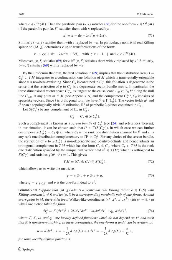
1402 V. Cortés et al.
where c ∈ C∞(M). Then the parabolic pair (u, l) satisfies (66) for the one-form κ ∈ �1(M)
iff the parabolic pair (u, l ′) satisfies them with κ replaced by:
κ ′ = κ + dc − λ(c2u + 2cl). (71)
Similarly (−u, l) satisfies them with κ replaced by−κ . In particular, a nontrivial real Killingspinor on (M, g) determines κ up to transformations of the form:
κ → ζκ + dc − λ(c2u + 2cl), with ζ ∈ {−1, 1} and c ∈ C∞(M).
Moreover, (u, l) satisfies (69) for κ iff (u, l ′) satisfies them with κ replaced by κ ′. Similarly,(−u, l) satisfies (69) with κ replaced by −κ .
By the Frobenius theorem, the first equation in (69) implies that the distribution ker(u) =C⊥u ⊂ T M integrates to a codimension one foliation of M which is transversally-orientablesince u is nowhere-vanishing. Since Cu is contained in C⊥u , this foliation is degenerate in thesense that the restriction of g to C⊥u is a degenerate vector bundle metric. In particular, thethree-dimensional vector space C⊥u,m is tangent to the causal cone Lm ⊂ TmM along the nullline Cu,m at any point m ∈ M (see Appendix A) and the complement C⊥u \ Cu consists ofspacelike vectors. Since l is orthogonal to u, we have l� ∈ �(C⊥u ). The vector fields u� andl� span a topologically trivial distribution �� of parabolic 2-planes contained in Cu .
Let S(C⊥u ) be any complement of Cu in C⊥u :
C⊥u = Cu ⊕ S(C⊥u ).
Such a complement is known as a screen bundle of C⊥u (see [24] and references therein);in our situation, it can be chosen such that l� ∈ �(S(C⊥u )), in which case we can furtherdecompose S(C⊥u ) = Cl ⊕ L , where Cl is the rank one distribution spanned by l� and L isany rank one distribution complementary to �� in C⊥u . For any choice of the screen bundle,the restriction of g to S(C⊥u ) is non-degenerate and positive-definite and hence admits anorthogonal complement in T M which has the form Cu ⊕ Cv , where Cv ⊂ T M is the rankone distribution spanned by the unique null vector field v� ∈ X(M) which is orthogonal toS(C⊥u ) and satisfies g(u�, v�) = 1. This gives:
T M = (Cv ⊕ Cu)⊕ S(C⊥u ), (72)
which allows us to write the metric as:
g = u ⊗ v + v ⊗ u + q, (73)
where q = g|S(C⊥u ) and v is the one-form dual to v�.
Lemma 5.10 Suppose that (M, g) admits a nontrivial real Killing spinor ε ∈ �(S) withKilling constant λ
2 �= 0 and let (u, l) be a corresponding parabolic pair of one-forms. Aroundevery point in M, there exist localWalker-like coordinates (xv, xu, x1, x2) with u� = ∂xu inwhich the metric takes the form:
ds2g = F (dxv)2 + 2Kdxvdxu + ωi dxvdxi + qi j dx
i dx j , (74)
where F , K, ωi and qi j are locally-defined functions which do not depend on xu and suchthat K is nowhere-vanishing. In these coordinates, the one-forms u and l can be written as:
u = Kdxv, l = − 1
2λd log(K)+ s dxv = − 1
2λd log(K)+ s
Ku,
for some locally-defined function s.
123
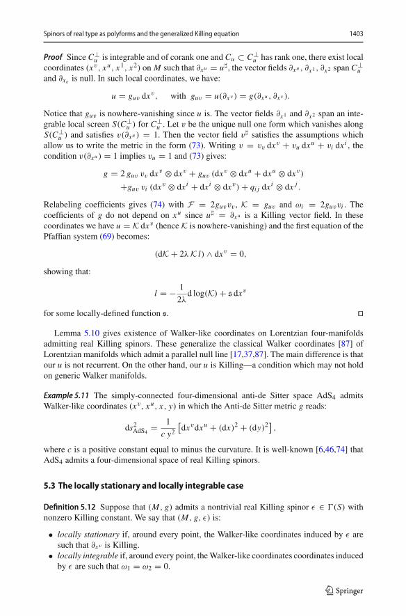
Spinors of real type as polyforms and the generalized Killing equation 1403
Proof Since C⊥u is integrable and of corank one and Cu ⊂ C⊥u has rank one, there exist localcoordinates (xv, xu, x1, x2) on M such that ∂xu = u�, the vector fields ∂xu , ∂x1 , ∂x2 span C
⊥u
and ∂xv is null. In such local coordinates, we have:
u = guv dxv, with guv = u(∂xv ) = g(∂xu , ∂xv ).
Notice that guv is nowhere-vanishing since u is. The vector fields ∂x1 and ∂x2 span an inte-grable local screen S(C⊥u ) for C⊥u . Let v be the unique null one form which vanishes alongS(C⊥u ) and satisfies v(∂xu ) = 1. Then the vector field v� satisfies the assumptions whichallow us to write the metric in the form (73). Writing v = vv dxv + vu dxu + vi dxi , thecondition v(∂xu ) = 1 implies vu = 1 and (73) gives:
g = 2 guv vv dxv ⊗ dxv + guv (dx
v ⊗ dxu + dxu ⊗ dxv)
+guv vi (dxv ⊗ dxi + dxi ⊗ dxv)+ qi j dxi ⊗ dx j .
Relabeling coefficients gives (74) with F = 2guvvv , K = guv and ωi = 2guvvi . Thecoefficients of g do not depend on xu since u� = ∂xu is a Killing vector field. In thesecoordinates we have u = K dxv (henceK is nowhere-vanishing) and the first equation of thePfaffian system (69) becomes:
(dK+ 2λK l) ∧ dxv = 0,
showing that:
l = − 1
2λd log(K)+ s dxv
for some locally-defined function s. ��Lemma 5.10 gives existence of Walker-like coordinates on Lorentzian four-manifolds
admitting real Killing spinors. These generalize the classical Walker coordinates [87] ofLorentzian manifolds which admit a parallel null line [17,37,87]. The main difference is thatour u is not recurrent. On the other hand, our u is Killing—a condition which may not holdon generic Walker manifolds.
Example 5.11 The simply-connected four-dimensional anti-de Sitter space AdS4 admitsWalker-like coordinates (xv, xu, x, y) in which the Anti-de Sitter metric g reads:
ds2AdS4 =1
c y2[dxvdxu + (dx)2 + (dy)2
],
where c is a positive constant equal to minus the curvature. It is well-known [6,46,74] thatAdS4 admits a four-dimensional space of real Killing spinors.
5.3 The locally stationary and locally integrable case
Definition 5.12 Suppose that (M, g) admits a nontrivial real Killing spinor ε ∈ �(S) withnonzero Killing constant. We say that (M, g, ε) is:
• locally stationary if, around every point, the Walker-like coordinates induced by ε aresuch that ∂xv is Killing.• locally integrable if, around every point, theWalker-like coordinates coordinates induced
by ε are such that ω1 = ω2 = 0.
123
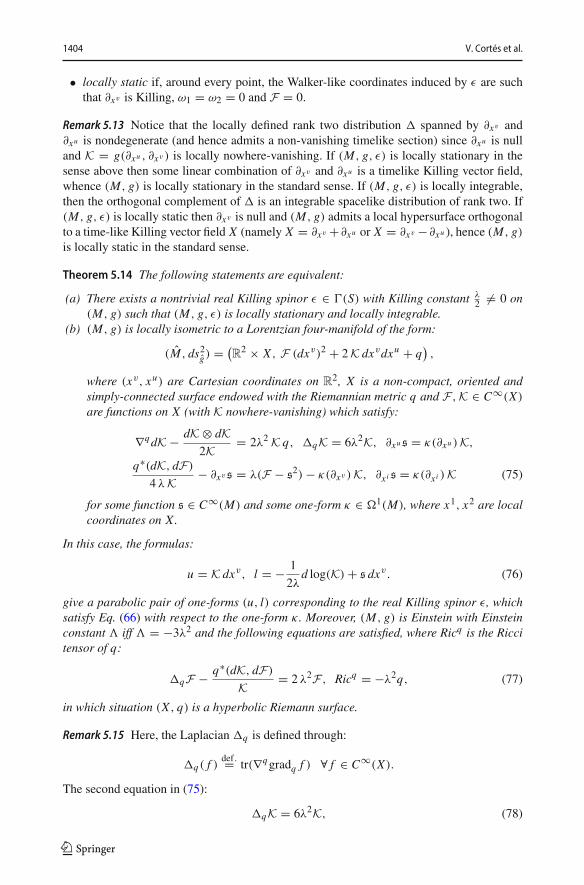
1404 V. Cortés et al.
• locally static if, around every point, the Walker-like coordinates induced by ε are suchthat ∂xv is Killing, ω1 = ω2 = 0 and F = 0.
Remark 5.13 Notice that the locally defined rank two distribution � spanned by ∂xv and∂xu is nondegenerate (and hence admits a non-vanishing timelike section) since ∂xu is nulland K = g(∂xu , ∂xv ) is locally nowhere-vanishing. If (M, g, ε) is locally stationary in thesense above then some linear combination of ∂xv and ∂xu is a timelike Killing vector field,whence (M, g) is locally stationary in the standard sense. If (M, g, ε) is locally integrable,then the orthogonal complement of � is an integrable spacelike distribution of rank two. If(M, g, ε) is locally static then ∂xv is null and (M, g) admits a local hypersurface orthogonalto a time-like Killing vector field X (namely X = ∂xv +∂xu or X = ∂xv −∂xu ), hence (M, g)is locally static in the standard sense.
Theorem 5.14 The following statements are equivalent:
(a) There exists a nontrivial real Killing spinor ε ∈ �(S) with Killing constant λ2 �= 0 on
(M, g) such that (M, g, ε) is locally stationary and locally integrable.(b) (M, g) is locally isometric to a Lorentzian four-manifold of the form:
(M, ds2g) =(R2 × X , F (dxv)2 + 2K dxvdxu + q
),
where (xv, xu) are Cartesian coordinates on R2, X is a non-compact, oriented and
simply-connected surface endowed with the Riemannian metric q and F,K ∈ C∞(X)
are functions on X (with K nowhere-vanishing) which satisfy:
∇qdK− dK⊗ dK2K
= 2λ2 K q, �qK = 6λ2K, ∂xu s = κ(∂xu )K,
q∗(dK, dF)
4 λK− ∂xvs = λ(F − s2)− κ(∂xv )K, ∂xi s = κ(∂xi )K (75)
for some function s ∈ C∞(M) and some one-form κ ∈ �1(M), where x1, x2 are localcoordinates on X.
In this case, the formulas:
u = K dxv, l = − 1
2λd log(K)+ s dxv. (76)
give a parabolic pair of one-forms (u, l) corresponding to the real Killing spinor ε, whichsatisfy Eq. (66) with respect to the one-form κ . Moreover, (M, g) is Einstein with Einsteinconstant � iff � = −3λ2 and the following equations are satisfied, where Ricq is the Riccitensor of q:
�qF − q∗(dK, dF)
K= 2 λ2F, Ricq = −λ2q, (77)
in which situation (X , q) is a hyperbolic Riemann surface.
Remark 5.15 Here, the Laplacian �q is defined through:
�q( f )def.= tr(∇qgradq f ) ∀ f ∈ C∞(X).
The second equation in (75):
�qK = 6λ2K, (78)
123
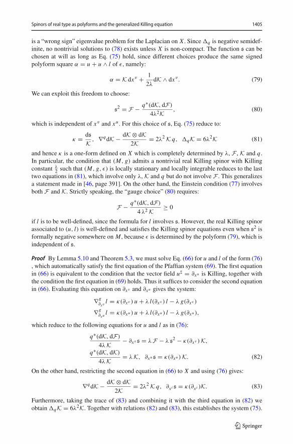
Spinors of real type as polyforms and the generalized Killing equation 1405
is a “wrong sign” eigenvalue problem for the Laplacian on X . Since�q is negative semidef-inite, no nontrivial solutions to (78) exists unless X is non-compact. The function s can bechosen at will as long as Eq. (75) hold, since different choices produce the same signedpolyform square α = u + u ∧ l of ε, namely:
α = K dxv + 1
2λdK ∧ dxv. (79)
We can exploit this freedom to choose:
s2 = F − q∗(dK, dF)
4λ2K, (80)
which is independent of xv and xu . For this choice of s, Eq. (75) reduce to:
κ = ds
K, ∇qdK− dK⊗ dK
2K= 2λ2 K q, �qK = 6λ2K (81)
and hence κ is a one-form defined on X which is completely determined by λ, F , K and q .In particular, the condition that (M, g) admits a nontrivial real Killing spinor with Killingconstant λ
2 such that (M, g, ε) is locally stationary and locally integrable reduces to the lasttwo equations in (81), which involve only λ, K and q but do not involve F . This generalizesa statement made in [46, page 391]. On the other hand, the Einstein condition (77) involvesboth F and K. Strictly speaking, the “gauge choice” (80) requires:
F − q∗(dK, dF)
4 λ2 K≥ 0
if l is to be well-defined, since the formula for l involves s. However, the real Killing spinorassociated to (u, l) is well-defined and satisfies the Killing spinor equations even when s2 isformally negative somewhere on M , because ε is determined by the polyform (79), which isindependent of s.
Proof By Lemma 5.10 and Theorem 5.3, we must solve Eq. (66) for u and l of the form (76), which automatically satisfy the first equation of the Pfaffian system (69). The first equationin (66) is equivalent to the condition that the vector field u� = ∂xu is Killing, together withthe condition the first equation in (69) holds. Thus it suffices to consider the second equationin (66). Evaluating this equation on ∂xv and ∂xu gives the system:
∇g∂xv
l = κ(∂xv ) u + λ l(∂xv ) l − λ g(∂xv )
∇g∂xu
l = κ(∂xu ) u + λ l(∂xu ) l − λ g(∂xu ),
which reduce to the following equations for u and l as in (76):
q∗(dK, dF)
4λK− ∂xvs = λF − λ s2 − κ(∂xv )K,
q∗(dK, dK)
4λK= λK, ∂xu s = κ(∂xu )K. (82)
On the other hand, restricting the second equation in (66) to X and using (76) gives:
∇qdK− dK⊗ dK2K
= 2λ2 K q, ∂xi s = κ(∂xi )K. (83)
Furthermore, taking the trace of (83) and combining it with the third equation in (82) weobtain�qK = 6λ2K. Together with relations (82) and (83), this establishes the system (75).
123
1406 V. Cortés et al.
Consider now the Einstein equation Ricg = � g on (M, g). The only non-trivial componentsare:
Ricg(∂xv , ∂xv ) = �F, Ricg(∂xu , ∂xv ) = �K, Ricg|T X = � q.
Direct computation gives:
Ricg(∂xv , ∂xv ) = −1
2�qF + 1
2Kq∗(dK, dF)− F
2K2 q∗(dK, dK),
Ricg(∂xv , ∂xu ) = −1
2�qK, Ricg|T X = Ricq − ∇
qdKdK
+ dK⊗ dK2K2 .
Combining these relations with (75), we conclude. ��Remark 5.16 Lorentzian four-manifolds admitting nontrivial real Killing spinors are super-symmetric configurations of four-dimensional N = 1 minimal AdS supergravity [28,81].Supersymmetric solutions of that theory are Lorentzian four-manifolds admitting nontrivialreal Killing spinors which satisfy the Einstein equation with negative cosmological constant.Hence Theorem 5.14 characterizes all locally integrable and locally stationary supersym-metric solutions of this theory. To our best knowledge, the classification of four-dimensionalLorentzian manifolds admitting real Killing spinors is currently open. Theorem 5.3 and [37]could be used to attack this problem in full generality.
Theorem 5.14 suggests a strategy to construct Lorentzian four-manifolds admitting realKilling spinors. Fix a simply-connected (generally incomplete) hyperbolic Riemann surface(X , q) and consider the eigenspace of the Laplacian on (X , q) with eigenvalue 6λ2. In thisspace, look for a function K which satisfies the first equation in (75). If such exists, it givesa real Killing spinor for any F ∈ C∞(X). Below, we give special classes of solutions when(X , q) is the Poincaré half-plane.
5.4 Special solutions from the Poincaré half-plane
Take:
(M, ds2g) =(
R2 ×H, F (dxv)2 + 2K dxvdxu + c
(dx)2 + (dy)2
y2
), (84)
where x, y are global coordinates on the Poincaré half-plane H = {(x, y) ∈ R
2 | y > 0}
and F,K are real-valued functions defined on H (with K nowhere-vanishing), while c > 0is a constant. Let q denote the metric c dx⊗dx+dy⊗dy
y2on H. Theorem 5.14 shows that such
(M, g) admits a real Killing spinor with Killing constant λ2 �= 0 iff:
∇qdK− dK⊗ dK2K
= 2λ2 K q, �qK = 6λ2K, (85)
in which case (M, g) is Einstein iff:
�qF − q∗(dK, dF)
K= 2 λ2F . (86)
Direct computation shows that Eq. (85) are equivalent with:
∂2xK−∂yKy= (∂xK)2
2K+ 2λ2c
y2K, ∂2yK+
∂yKy= (∂yK)2
2K+ 2λ2c
y2K,
∂2xyK+∂xKy= ∂xK∂yK
2K, y2
(∂2xK+ ∂2yK
)= 6 λ2cK.
123
Spinors of real type as polyforms and the generalized Killing equation 1407
This gives the following:
Corollary 5.17 The Lorentzian four-manifold (84) admits a nontrivial real Killing spinor withKilling constant λ
2 �= 0 iff:
∂2yK+∂yKy= (∂yK)2
2K+ 2λ2c
y2K, ∂2xyK+
∂xKy= ∂xK∂yK
2K,
(∂xK)2 + (∂yK)2 = 4 λ2c
y2K2, y2
(∂2xK+ ∂2yK
)= 6 λ2.cK. (87)
In this case, it is Einstein iff F satisfies (86).
Choosing F to not satisfy (86) produces large families of non-Einstein Lorentzian four-manifolds admitting real Killing spinors.
Example 5.18 TakingK = F = cy2
gives a solution of (87) iff c λ2 = 1. Hence the Lorentzianfour-manifold:
(M, ds2g) =(
R2 ×H,
1
λ2y2[(dxv)2 + 2 dxvdxu + (dx)2 + (dy)2
])
admits a real Killing spinor. This is the AdS4 space with metric written in horosphericcoordinates [44], which is well-known to admit the maximal number (namely four) of realKilling spinors [11].
More examples can be constructed by solving in more generality the eigenvector problemfor the Laplace operator of the Poincaré half plane and checking which solutions satisfy thefirst equation in (85). We illustrate this by constructing solutions obtained through separationof variables. Set:
K = kx ky,
where kx ∈ C∞(H) depends only on x and ky ∈ C∞(H) depends only on y. The secondequation in (87) gives:
kx
(ky + 2ky
y
)= 0, (88)
where the dot denotes derivation with respect to the corresponding variable. When kx = 0,Eq. (87) reduce to:
∂yK+ 2
yK = 0, λ2c = 1,
with general solution K = c0y−2 (where c0 �= 0 is a constant). If kx �= 0, then (88) givesky + 2ky
y = 0, so ky = c0y−2 for a non-zero constant c0. Using this in (87) gives kx = 0, acontradiction. Hence every Lorentzian four-manifold of the form:
(M, ds2g) =(
R2 ×H, F (dxv)2 + 2 c0
dxvdxu
y2+ (dx)2 + (dy)2
λ2y2
)(89)
with F a smooth function admits nontrivial real Killing spinors. This gives large familiesof non-Einstein Lorentzian four-manifolds carrying real Killing spinors by taking F to be
123
1408 V. Cortés et al.
generic. The Lorentzian manifold (89) is Einstein when Eq. (86) is satisfied, which forK = c0y−2 reads:
y2(∂2xF + ∂2yF
)+ 2 y ∂yF = 2F . (90)
To study (90), we try the separated Ansatz:
F = fx fy,
where fx ∈ C∞(H) depends only on x and fy ∈ C∞(H) depends only on y. Equation (90)gives:
fxfx= c2 = f y
fy+ 2 f y
y fy− 2
y2(91)
for some c ∈ R. If c = 0, this is solved by:
fx = a1 + a2x, fy = a3y + a4y2
,
where a def.= (a1, . . . , a4) ∈ R4. This gives the following family of Einstein Lorentzian
metrics on R2 ×H admitting real Killing spinors, where we eliminated c0 by rescaling xu :
dsg = (a1 + a2x)
(a3y + a4
y2
)(dxv)2 + dxvdxu
y2+ (dx)2 + (dy)2
λ2y2. (92)
For a1 = a2 = a3 = a4 = 0 we recover the AdS4 metric written in horospheric coordinates.Thus (92) gives a four-parameter deformation of AdS4. Every choice a ∈ R
4 produces anEinstein metric on R
2 ×H with Einstein constant� = −3λ2 admitting real Killing spinors.If c �= 0, the first equation in (91) gives:
fx = a1ecx + a2e
−cx
with a1, a2 ∈ R. On the other hand, the equation for fy can be written as:
y2 f y + 2y fy + (c2y2 − 2) fy = 0,
being the radial part of the Helmholtz equation in spherical coordinates. Its general solutionis a linear combination of the spherical Bessel functions BY and BJ:
fy = a3BY(cy)+ a4BJ(cy),
where a3, a4 ∈ R. We have:
BJ(cy) = sin(cy)
c2y2− cos(cy)
cy, BY(cy) = −cos(cy)
c2y2− sin(cy)
cy,
whence:
ds2g = (a1ecx + a2e
−cx ) [a3BY(cy)+ a4BJ(cy)] (dxv)2 + dxvdxu
y2+ (dx)2 + (dy)2
λ2y2.
This gives a four-parameter family (parameterized by (a1, a2, a3, a4) ∈ R4) of Lorentzian
Einstein metrics on R2 ×H admitting real Killing spinors.
Remark 5.19 When a1a2 �= 0 and a3 �= 0, the Lorentzian four-manifolds constructed aboveare not isometric to AdS4, since their Weyl tensor is non-zero and their Riemann tensor isnot parallel.
123
Spinors of real type as polyforms and the generalized Killing equation 1409
6 Supersymmetric heterotic configurations
In this section we consider generalized constrained Killing spinors in an abstract form ofheterotic supergravity (inspired by [39]), which is parameterized by a triplet (M, P, c), whereM is a spin open four-manifold, P is a principal bundle over M with compact semi-simpleLie structure groupG and c is an AdG -invariant, symmetric and non-degenerate inner product
on the Lie algebra g ofG. Let gPdef.= P×AdG g be the adjoint bundle of P . The Killing spinor
equations of heterotic supergravity couple a strongly spinnable Lorentzian metric g on M(taken to be of “mostly plus” signature), a closed one-form ϕ ∈ �1(M), a three-form H ∈�3(M) and a connection A on P . This system of partial differential equations characterizessupersymmetric configurations of the theory defined by (M, P, c). For simplicity, we assumeH1(M,Z2) = 0, although this assumption can be relaxed. We refer the reader to Appendix 6for certain details.
6.1 Supersymmetric heterotic configurations
Let us fix a triple (M, P, c) as above, where H1(M,Z2) = 0. For every strongly-spinnablemetric g of signature (3, 1) on M , let Sg = (S, �,B ) be a paired real spinor bundle on(M, g), where the admissible pairing B is skew-symmetric and of negative adjoint type.With our assumptions, Sg is unique up to isomorphism of paired spinor bundles, combinedwith a rescaling of B by a non-zero constant. Let FA ∈ �2(gP ) denote the curvature formof a connection A on P . As explained in Appendix 6, g and c induce a symmetric morphism
of vector bundles c(− ∧ −) : �(M, gp) ⊗ �(M, gp) → �(M), where �(M, gp)def.=
�(M) ⊗ gP . For any 3-form H ∈ �3(M), let ∇H be the natural lift to Sg of the uniquemetric connection on (M, g) with totally skew-symmetric torsion given by −H .
Definition 6.1 A heterotic configuration for (M, P, c) is an ordered quadruplet (g, ϕ, H , A),where g is a strongly-spinnable Lorentzian metric on M , ϕ ∈ �1(M) is a closed one-form,H ∈ �3(M) is a three-form and A ∈ AP is a connection on P such that themodified Bianchiidentity holds:
dH = c(FA ∧ FA). (93)
The configuration is called supersymmetric if there exists a nontrivial spinor ε ∈ �(Sg) suchthat:
∇H ε = 0, ϕ · ε = H · ε, FA · ε = 0. (94)
Remark 6.2 Equations (94) encode vanishing of the gravitino, dilatino and gaugino super-symmetry variations. Since we work in Lorentzian signature, supersymmetric configurationsneed not solve the equations of motion (which are given in Appendix 6). However, the studyof supersymmetric configurations is a first step toward classifying supersymmetric solutions.The study of supersymmetric solutions this theory in the physical case of ten Lorentziandimensions was pioneered in [48–50], where their local structure was characterized. Thelast equation in (94) is formally identical to the spinorial characterization of instantons inRiemannian signature and dimensions from four to eight.
123
1410 V. Cortés et al.
6.2 Characterizing supersymmetric heterotic configurations through differentialforms
The metric connection ∇H is given by (see Appendix 6 for notation):
∇HY X = ∇g
Y X −1
2H �(X , Y ) ∀X , Y ∈ X(M),
where ∇g is the Levi-Civita connection of (M, g) and H � is H viewed as a T M-valuedtwo-form. Hence the first equation in (94) can be written as:
∇gXε −
1
4H(X) · ε = 0 ∀ X ∈ X(M),
where H(X)def.= ιX H ∈ �2(M). This shows that ε is a generalized Killing spinor relative
to the connection D = ∇S −A on S, where:
AXdef.= �−1� (A) = 1
4H(X) = 1
4(∗ρ)(X) = 1
4∗ (ρ ∧ X �) ∀X ∈ X(M)
and we defined ρdef.= ∗H ∈ �1(M). The second and third conditions in (94) are linear
algebraic constraints on ε. Hence the first three equations of (94) state that ε is a constrainedgeneralized Killing spinor (see Definition 4.15). As in Sects. 3.6.3 and 4.6, consider a signedpolyform square of ε:
α = u + u ∧ l,
where (u, l) is a parabolic pairs of one-forms.
Lemma 6.3 (g, ϕ, H , A, ε) satisfies the second equation in (94) (the dilatino equation) iff:
ϕ ∧ u = − ∗ (ρ ∧ u), ϕ ∧ u ∧ l = g∗(ρ, l) ∗ u, g∗(ϕ, l) u = ∗(l ∧ u ∧ ρ),
g∗(u, ϕ) = 0, g∗(u, ρ) = 0, g∗(ρ, ϕ) = 0,
where ρdef.= ∗H.
Proof By Proposition 3.26, the dilatino equation holds iff:
ϕ � α = H � α, (95)
where α = u + u ∧ l is a signed polyform square of ε. We compute:
ϕ � α = g∗(ϕ, u)+ ϕ ∧ u + ϕ ∧ u ∧ l + g∗(ϕ, u) l − g∗(ϕ, l) u,H � α = ν � ρ � α = g∗(ρ, u) ν − ∗(ρ ∧ u)− ∗(l ∧ u ∧ ρ)+ g∗(ρ, u) ∗ l + g∗(ρ, l) ∗ u,where in the second equation we used (37) to rewrite the geometric product in terms of ρ.Separating degrees in (95) and using these relations gives the conclusion. ��
Lemma 6.4 (g, ϕ, H , A, ε) satisfies the third equation in (94) (the gaugino equation) iff:
FA = u ∧ χA, (96)
where χA ∈ �(u⊥ ⊗ gP ) is a gP-valued one-form orthogonal to u.
123
Spinors of real type as polyforms and the generalized Killing equation 1411
Proof By Proposition 3.26, the gaugino equation holds iff:
α � FA = u � FA + u � l � FA = 0. (97)
Expanding the geometric product gives:
α � FA = u ∧ FA + ιu FA + u ∧ l ∧ FA − l ∧ ιu FA + u ∧ ιl FA + ιu ιl FA = 0.
Hence separating degrees in (97) gives the system:
u ∧ FA = 0, ιu FA = 0,
which is solved by (96). ��Lemma 6.5 (g, ϕ, H , A, ε) satisfies the first equation in (94) (the gravitino equation) iff:
∇gu = 1
2∗ (ρ ∧ u), ∇gl = 1
2∗ (ρ ∧ l)+ κ ⊗ u. (98)
where κ ∈ �1(M) and ρdef.= ∗H. In this case, u� ∈ X(M) is a Killing vector field.
Proof By Theorem 4.26, the gravitino equation holds iff:
∇gv (u + u ∧ l) = 1
4[H(v) � (u + u ∧ l)− (u + u ∧ l) � H(v)] ∀ v ∈ X(M),
which reduces to the followingupon expanding the geometric product and separating degrees:
2∇gv u + H(v, u) = 0, 2∇g
v (u ∧ l)+ H(v, u) ∧ l + u ∧ H(v, l) = 0.
This system is equivalent with:
2∇gv u + H(v, u) = 0, 2∇g
v l + H(v, l)− 2κ(v)u = 0 ∀ v ∈ X(M)
for some one-form κ ∈ �1(M). In turn, this is equivalent with (98). ��Theorem 6.6 A quadruplet (g, ϕ, H , A) is a supersymmetric heterotic configuration for(M, P, c) iff there exists a parabolic pair of one-forms (u, l) such that the following equations
(where ρdef.= ∗H ∈ �1(M)) are satisfied:
ϕ ∧ u = ∗(ρ ∧ u), ϕ ∧ u ∧ l = −g∗(ρ, l) ∗ u, − g∗(ϕ, l) u = ∗(l ∧ u ∧ ρ),
g∗(u, ϕ) = 0, g∗(u, ρ) = 0, g∗(ρ, ϕ) = 0, FA = u ∧ χA,
∇gu = 1
2u ∧ ϕ, ∇gl = 1
2∗ (ρ ∧ l)+ κ ⊗ u, d∗ρ = 0, (99)
for some one-form κ ∈ �1(M) and some gP-valued one-form χA ∈ �1(M, gP ) whichis orthogonal to u. In this case, u� ∈ X(M) is a Killing vector field and the distributionker u ⊂ T M integrates to a transversely-orientable codimension one foliation of M.
Proof By Lemmas 6.3, 6.4 and 6.5, it suffices to prove the last equation in the third line of(99). The modified Bianchi identity can be written as:
d ∗ ρ = ∗2c(FA ∧ FA),
and gives:
d∗ρ = c(ιuχA, ιuχA) = c(χA(u), χA(u)) = 0,
123
1412 V. Cortés et al.
because χA is orthogonal to u. The first equation in the the third line of (99) amounts to:
Lu�g = 0, du = 1
8u ∧ ϕ,
showing thatu� isKilling and the distribution ker u ⊂ T M is integrable, giving a transversely-orientable foliation Fu ⊂ M of codimension one. ��
6.3 Some examples
Example 6.7 Let:
(M, ds2g) =(R2 × X , 2 dxvdxu + q(xv)
),
where q(xv) is a flat Riemannianmetric on X for all xv ∈ R and take P to be the unit principalbundle over M . Consider the spinor ε corresponding to the pair (u, l), where u = dxv andl = l(xv) depends on xv . Finally, take:
ϕ = � u, ρ = 0,
where � ∈ C∞(R2 × X). A short computation shows that Eq. (99) reduce to:
∇gl = κ ⊗ dxv.
Applying this to ∂xv , ∂xu and restricting to T X gives:
∇gxv l = ∂xv l − 1
2l��∂xvq(xv) = 0, κ(∂xv ) = 0, κ(∂xu ) = 0,
∇gl|T ∗X = ∇ql − 1
2l��∂xvq(xv)dxv = (κX − ∗q(xv)l)⊗ dxv,
where κXdef.= κ|T X . This implies:
∇ql = 0, κX = ∗q(xv)l − 1
2l��∂xvq(xv),
showing that (X , q(xv)) is flat for all xv ∈ R. The only remaining non-trivial condition is:
∂xv l = 1
2l��∂xvq(xv). (100)
This is a linear first order ordinary differential equation for the function xv → l(xv). Forevery choice of parallel vector field on (X , q(xv0 )) with fixed (xv0 , x
u0 ) ∈ R
2, its solutionwith the corresponding initial condition determines a one-parameter family of one forms{l(xv)}xv∈R on (X , q(xv)). Assuming for instance that X is simply connected and that q(xv)satisfies:
∂xvq(xv) = 2F(xv) q(xv),
for some function F(xv) depending only on xv , then the explicit solution is:
l(xv) = e∫F(xv)l0,
where l0 is parallel vector field on (X , q(xv0 )) and we canonically identify the tangent vectorspaces of {(xv, xu)} × X at different points (xv, xu).
123
Spinors of real type as polyforms and the generalized Killing equation 1413
Remark 6.8 Heterotic solutions with exact null dilaton were considered before (see [13]).As remarked earlier, a supersymmetric heterotic configuration need not be a solution ofthe equation of motion given in Appendix B. The classification of (geodesically complete)supersymmetric heterotic solutions on a Lorentzian four-manifold and the diffeomorphismtype of four-manifolds admitting such solutions for fixed principal bundle topology is an openproblem. Appendix B gives a brief formulation of abstract bosonic heterotic supergravity andits Killing spinor equations.
Acknowledgements The work of C. I. L. was supported by Grant IBS-R003-S1. The work of C. S. S. issupported by the Humboldt Research Fellowship ESP 1186058 HFST-P from the Alexander von HumboldtFoundation. The research of V.C. and C.S.S. was partially funded by the Deutsche Forschungsgemeinschaft(DFG,GermanResearchFoundation) underGermany’sExcellenceStrategy—EXC2121QuantumUniverse—390833306.
Funding Open Access funding enabled and organized by Projekt DEAL.
Open Access This article is licensed under a Creative Commons Attribution 4.0 International License, whichpermits use, sharing, adaptation, distribution and reproduction in any medium or format, as long as you giveappropriate credit to the original author(s) and the source, provide a link to the Creative Commons licence,and indicate if changes were made. The images or other third party material in this article are included in thearticle’s Creative Commons licence, unless indicated otherwise in a credit line to the material. If material isnot included in the article’s Creative Commons licence and your intended use is not permitted by statutoryregulation or exceeds the permitted use, you will need to obtain permission directly from the copyright holder.To view a copy of this licence, visit http://creativecommons.org/licenses/by/4.0/.
Appendix A: Parabolic 2-planes and degenerate complete flags in R3,1
Let (V , h) be a four-dimensional Minkowski space of “mostly plus” signature. A non-zerosubspaceW ⊂ V ∗ is called degenerate or nondegenerate according to whether the restrictionh∗W of h∗ toW is a degenerate or non-degenerate quadratic form. A non-degenerate subspaceW is called:
• positive or negative definite, if the restriction h∗W to W is positive or negative negativedefinite, respectively• hyperbolic, if the restriction of h∗ to W is not positive or negative definite.
Notice that W is partially isotropic (i.e. contains nonzero null vectors) iff it is degenerateor hyperbolic. Let L denote the cone of causal (i.e. non-spacelike) vectors in (V ∗, h∗). Anon-zero subspace W ⊂ V ∗ is:
• hyperbolic iff dim(W ∩ L) > 1, i.e. iff W meets L along a sub-cone of the latter whichhas dimension at least two.• degenerate iff dim(W ∩ L) = 1, i.e. iff W is tangent to L along a null line• non-degenerate iff W ∩ L = {0}, in which case W is spacelike (i.e. positive definite).
A degenerate subspace W of V ∗ contains no timelike vectors and the set of its null vectors
coincides with the kernel Kh(W )def.= ker(h∗W ); accordingly, W decomposes as:
W = Kh(W )⊕U ,
where Kh(W ) = ker(h∗W ) coincides with the unique null line contained in W and U isa spacelike subspace of V ∗ which is orthogonal to Kh(W ). In particular, we have W ⊂Kh(W )⊥. For example, a 2-plane � ⊂ V ∗ can be spacelike, hyperbolic or degenerate,
123
1414 V. Cortés et al.
according towhether h∗� is positive-definite, non-degenerate of signature (1, 1) or degenerate.In the latter case, � is called a parabolic 2-plane.
Definition A.2 A complete flag 0 ⊂ W(1) ⊂ W(2) ⊂ W(3) ⊂ V ∗ is called degenerate if W(i)
is a degenerate subspace of (V ∗, h∗) for each i = 1, 2, 3.
Notice that a complete flag 0 ⊂ W(1) ⊂ W(2) ⊂ W(3) ⊂ V ∗ is determined by the
increasing sequence of vector spacesW•def.= (W(1),W(2),W(3)). Such a flag is degenerate iff
W(2) and W(3) are tangent to the light cone of (V ∗, h∗) along the line W(1) (whence W(1) isa null line).
Proposition A.3 There exists a natural bijection between the set of parabolic 2-planes andthe set of degenerate complete flags in (W ∗, h∗). This associates to each parabolic 2-plane� ⊂ V ∗ the unique degenerate complete flag 0 ⊂ W(1) ⊂ W(2) ⊂ W(3) ⊂ V ∗ withW(2) = �, which is given by:
W(1) = Kh(�), W(2) = �, W(3) = Kh(�)⊥. (101)
Proof Let 0 ⊂ W(1) ⊂ W(2) ⊂ W(3) ⊂ V ∗ be a degenerate complete flag. Then the 2-
plane �def.= W(2) is degenerate, i.e. parabolic. Since the subspace W(1) of W(2) = � is
degenerate and one-dimensional, it is a null line and hence coincides with Kh(�). SinceW(3) is degenerate, the one-dimensional subspace Kh(W(3)) is the unique null line containedin W(3) and hence coincides with W(1). We thus have W(3) ⊂ W⊥(1). This inclusion is an
equality because dimW⊥(1) = dim V ∗ − 1 = 3 = dimW(3). Hence any degenerate completeflag has the form (101) for a unique parabolic 2-plane �, namely � = W(2). It is clear thatthe correspondence thus defined is a bijection. ��Definition A.4 A co-oriented degenerate complete flag in (V ∗, h∗) is a pair (W•, L), whereW• = (W(1),W(2),W(3)) is a degenerate complete flag in (V ∗, h∗) and L is a co-orientationof the parabolic two-plane W(2).
Corollary 3.36 and Proposition A.3 imply the following reformulation of Theorem 3.34:
Theorem A.5 There exists a natural bijection between P(�) and the set of all co-orienteddegenerate complete flags in (V ∗, h∗).
Appendix B: Heterotic supergravity in four Lorentzian dimensions
Let G be a compact semisimple real Lie group whose Lie algebra we denote by g andwhose adjoint representation we denote by AdG : G → GL(g). Let g = g1 ⊕ · · · ⊕ gk bethe decomposition of g into simple Lie algebras. Then any AdG -invariant non-degeneratesymmetric pairing c on g can be written as:
c = c1B1 ⊕ · · · ⊕ ck Bk,
where Bj is the Killing form of g j and c j are non-zero constants.
Definition B.1 A four-dimensional heterotic datum of type G on M is a triplet (M, P, c),where M is an oriented open four-manifold, P is a principal bundle over M and c is anon-degenerate symmetric and AdG -invariant bilinear pairing on g.
123
Spinors of real type as polyforms and the generalized Killing equation 1415
Let (M, P, c) be a four-dimensional heterotic datum. Let gPdef.= P ×AdG g be the adjoint
bundle of Lie algebras of P and AP be the affine space of connections on P . For anyconnection A ∈ AP , let FA ∈ �2(M, gP ) denote the curvature form of A. Let cP be thepairing induced by c on the adjoint bundle gP . Since c is AdG -invariant, the latter can beviewed as a morphism of vector bundles:
cP : gP ⊗ gP → RM ,
where RM is the trivial real line bundle on M . Let �(M, gP )def.= �(M)⊗ gP and consider
the vector bundle morphism:
c(− ∧−) def.= ∧⊗ c : �(M, gP )⊗�(M, gP )→ �(M),
where ∧ : �(M) ⊗ �(M) → �(M) is the wedge product. Let Met3,1(M) be the set ofmetrics of signature (3, 1) defined on M . Let:
〈, 〉g : �(M)×�(M)→ RM and 〈, 〉g,c = 〈, 〉g ⊗ cP : �(M, gP )× (�(M, gP )→ RM
be themetrics induced by g ∈ Met3,1(M) and cP on the vector bundles�(M) and�(M, gP ).Consider the symmetric bilinear maps corresponding to the vector bundle morphisms:
◦ : �(M)⊗�(M)→ T ∗M ⊗ T ∗M and
c(− ◦ −) : �(M, gP )⊗�(M, gP )→ T ∗M ⊗ T ∗M
whose action on global sections is given by:
(ω ◦ η)(X , Y )def.= 〈ιXω, ιY η〉g ∀ω, η ∈ �(M) ∀X , Y ∈ X(M)
c(α ◦ β)(X , Y )def.= 〈ιXα, ιYβ〉g,c ∀α, β ∈ �(M, gP ) ∀X , Y ∈ X(M).
For a three-form H ∈ �3(M) and the curvature FA ∈ �2(gP ) of a connection A ∈ AP , wehave:
(H ◦ H)(X , Y ) = 〈ιX H , ιY H〉g ∀X , Y ∈ X(M),
c(FA ◦ FA)(X , Y ) = 〈ιX FA, ιY FA〉g,c ∀X , Y ∈ X(M).
Remark B.2 Pick a nonempty open subset U ⊂ M which supports local coordinates{xi }i=1,...,4 ofM aswell as a local g-orthonormal frame {ei }i=1,...,4 of T M and a c-orthogonallocal frame {Ta}a=1,...,rkg of gP such that c(Ta, Tb) = δab εa , where εa ∈ {−1, 1}. Then thefollowing relations hold on U :
c(FA ∧ FA) = εa FaA ∧ Fa
A, c(FA ◦ FA)i j = εa(FaA)im (Fa
A) jk gmk,
(H ◦ H)i j = HilmH lmj ,
where FA = FaATa and we use Einstein summation over i, j, l,m = 1, . . . , 4 and over
a = 1, . . . rk g.
Let �1cl(M) be the space of closed one-forms defined on M .
Definition B.3 A bosonic heterotic configuration of (M, P, c) is a quadruplet (g, ϕ, H , A) ∈Met3,1(M)×�1
cl(M)×�3(M)×AP which satisfies the modified Bianchi identity:
dH = c (FA ∧ FA) . (102)
123
1416 V. Cortés et al.
The one-form ϕ ∈ �1cl(M) is called the dilatonic one-form of the bosonic heterotic
configuration. On sufficiently small non-empty open subsets U ⊂ M , it can be written asϕ = dφ, where the locally defined function φ ∈ C∞(U ) corresponds to the dilaton of thephysics literature.
Definition B.4 A bosonic heterotic configuration (g, ϕ, H , A) of (M, P, c) is called bosonicheterotic solution if it satisfies the equations of motion:
Ricg + ∇gϕ − 1
4H ◦ H − c(FA ◦ FA) = 0,
d∗H + ιϕH = 0,
dA ∗ FA − ϕ ∧ ∗FA + FA ∧ ∗H = 0,
d∗ϕ + 〈ϕ, ϕ〉g − 〈H , H〉g − 〈FA, FA〉g,c = 0.
Let Conf(M, P, c) and Sol(M, P, c) ⊂ Conf(M, P, c) be the sets of bosonic configura-tions and solutions of the heterotic datum (M, P, c).
Remark B.5 If G is the trivial group, then P is the unit principal bundle over M , which hastotal space M and projection given by the identity map idM . In this case, c vanishes (as doesany connection on P) and the set of bosonic configurations reduces to:
Conf0(M) = Met3,1(M)�1cl(M)�3
cl(M),
since the modified Bianchi identity requires dH = 0. Moreover, the equations of motionreduce to:
Ricg +∇gϕ − 1
4H ◦ H = 0, d∗H + ιϕH = 0,
d∗ϕ + 〈ϕ, ϕ〉g − 〈H , H〉g = 0.(103)
This particular case is known as NS-NS supergravity.
For any three-form H on M , let ∇H be the unique g-compatible connection on T M withtotally skew-symmetric torsion given by T = H �, where H � ∈ �(T ∗M ⊗ T ∗M ⊗ T M) isdefined through:
H �(X , Y ) = (ιY ιX H)� ∈ X(M) ∀X , Y ∈ X(M).
Here � denotes raising of indices with respect to g. This connection is given by:
∇H = ∇g − 1
2H �.
Assume that M admits strongly spinnable Lorentzian metrics, whose space we denote byMetss3,1(M). We shall assume for simplicity that H1(M,Z2) = 0, although this can berelaxed. For any g ∈ Metss3,1(M), let (Sg, �g) be a spinor bundle on (M, g). The assumption
H1(M,Z2) = 0 implies that this spinor bundle is unique up to isomorphism.
Definition B.6 A bosonic heterotic configuration (g, ϕ, H , A) ∈ Conf(M, P, c) is calledsupersymmetric if g ∈ Metss3,1(M) and there exists a nontrivial spinor ε ∈ �(Sg) whichsatisfies the Killing spinor equations:
∇H ε = 0, ϕ · ε = H · ε = 0, FA · ε = 0. (104)
A similar formulation can be given for heterotic supergravity on a ten-dimensional openmanifold.
123
Spinors of real type as polyforms and the generalized Killing equation 1417
References
1. Agricola, I., Friedrich, T.: The SRNI lectures on non-integrable geometries with torsion. Arch. Math. 42,5–84 (2006)
2. Agricola, I., Friedrich, T.: 3-Sasakian manifolds in dimension seven, their spinors and -structures. J.Geom. Phys. 60(2), 326–332 (2010)
3. Agricola, I., Höll, J.: Cones of G manifolds and Killing spinors with skew torsion. Ann. Mat. Pura Appl.194(3), 673–718 (2015)
4. Alekseevsky, D.V., Cortés, V.: Classification of N-(super)-extended Poincaré algebras and bilinear invari-ants of the spinor representation of Spin(p, q). Commun. Math. Phys. 183(3), 477–510 (1997)
5. Alekseevsky,D.V., Cortés, V., Devchand, C., Proyen,A.V.: Polyvector super-Poincaré algebras. Commun.Math. Phys. 253(2), 385–422 (2005)
6. Alonso-Alberca, N., Lozano-Tellechea, E., Ortin, T.: Geometric construction of Killing spinors and super-symmetry algebras in homogeneous space-times. Class. Quantum Gravity 19, 6009 (2002)
7. Babalic, E.M., Lazaroiu, C.I.: The landscape of G-structures in eight-manifold compactifications of M-theory. JHEP 1511, 007 (2015)
8. Bär, C.: Real Killing spinors and holonomy. Commun. Math. Phys. 154, 509–521 (1993)9. Bär, C., Gauduchon, P., Moroianu, A.: Generalized cylinders in semi-Riemannian and spin geometry.
Math. Z. 249, 545–580 (2005)10. Bellorin, J., Ortin, T.: All the supersymmetric configurations of N = 4, d = 4 supergravity. Nucl. Phys. B
726, 171–209 (2005)11. Bellorin, J., Ortin, T.: A note on simple applications of the Killing spinor identities. Phys. Lett. B 616,
118–124 (2005)12. Berezin, F.A., Marinov, M.S.: Particle spin dynamics as the Grassmann variant of classical mechanics.
Ann. Phys. 104, 336–362 (1977)13. Bergshoeff, E.A., Kallosh, R., Ortin, T.: Supersymmetric string waves. Phys. Rev. D 47, 5444 (1993)14. Bernal, A.N., Sanchez, M.: On Smooth Cauchy hypersurfaces and Geroch’s splitting theorem. Commun.
Math. Phys. 243, 461–470 (2003)15. Blaine Lawson, H., Michelsohn, M.-L.: Spin geometry. Princeton Mathematical Series, vol. 38 (1990)16. Bohle, C.: Killing spinors on Lorentzian manifolds. J. Geom. Phys. 45(3–4), 285–308 (2003)17. Brozos-Vázquez, M., García-Río, E., Gilkey, P., Nikcevic, S., Vázquez-Lorenzo, R.: The geometry of
Walker manifolds. Synth. Lect. Math. Stat. 2, 1 (2009)18. Bryant, R.L.: Pseudo-Riemannian metrics with parallel spinor fields and vanishing Ricci tensor. Sémin.
Congr. 4(53), 53–94 (2000). Soc. Math. France, Paris19. Caldarelli, M.M., Klemm, D.: All supersymmetric solutions of N = 2, D = 4 gauged supergravity. JHEP
0309, 019 (2003)20. Chevalley, C.: The Algebraic Theory of Spinors. Columbia University Press, New York (1954)21. Chevalley, C.: The construction and study of certain important algebras, Math. Soc. Japan 1955. In:
Collected Works, vol. 2. Springer, Berlin (1997)22. Coimbra, A., Strickland-Constable, C.: Supersymmetric backgrounds, the Killing superalgebra, and gen-
eralised special holonomy. JHEP 1611, 063 (2016)23. Conti, D., Salamon, S.: Generalized Killing spinors in dimension 5. Trans. Am. Math. Soc. 359(11),
5319–5343 (2007)24. Duggal, K.L., Sahin, B.: Differential Geometry of Lightlike Submanifolds, Frontiers in Mathematics.
Birkhäuser (2018)25. Dunajski, M.: Anti-self-dual four-manifolds with a parallel real spinor. Proc. Math. Phys. Eng. Sci.
458(2002), 1205–1222 (2021)26. Figueroa-O’Farrill, J.M.: The Homogeneity conjecture for supergravity backgrounds. J. Phys. Conf. Ser.
175, 012002 (2009)27. Figueroa-O’Farrill, J.M., Papadopoulos, G.:Maximally supersymmetric solutions of ten-dimensional and
eleven-dimensional supergravities. JHEP 0303, 048 (2003)28. Freedman, D.Z., Van Proeyen, A.: Supergravity, CambridgeMonographs onMathematical Physics, Cam-
bridge (2012)29. Friedrich, T.: On the spinor representation of surfaces in Euclidean 3-space. J. Geom. Phys. 28(1–2),
143–157 (1998)30. Friedrich, T.: Dirac operators in Riemannian geometry, Graduate Studies in Mathematics, vol. 25. AMS,
Providence (2000)31. Friedrich, T., Ivanov, S.: Parallel spinors and connections with skew symmetric torsion in string theory.
Asian J. Math. 6, 303–336 (2002)
123

1418 V. Cortés et al.
32. Friedrich, T., Kath, I.: 7-Dimensional compact Riemannian manifolds with Killing spinors. Commun.Math. Phys. 133, 543–561 (1990)
33. Friedrich, T., Kim, E.C.: The Einstein–Dirac equation on Riemannian spin manifolds. J. Geom. Phys.33(1–2), 128–172 (2000)
34. Friedrich, T., Kim, E.C.: Some remarks on theHijazi inequality and generalizations of theKilling equationfor spinors. J. Geom. Phys. 37(1–2), 1–14 (2001)
35. Friedrich, T., Trautman, A.: Spin spaces, Lipschitz groups and spinor bundles. Ann. Glob. Anal. Geom.18(3–4), 221–240 (2000)
36. Galaev, A.S.: Examples of Einstein spacetimes with recurrent null vector fields. Class. Quantum Gravity28, 175022 (2011)
37. Galaev,A.S., Leistner, T.: On the local structure of Lorentzian Einsteinmanifoldswith parallel distributionof null lines. Class. Quantum Gravity 27, 225003 (2010)
38. Garcia-Fernandez, M.: Lectures on the Strominger system. Travaux Math. XXIV, 7–61 (2016)39. Garcia-Fernandez, M., Rubio, R., Tipler, C.: Infinitesimal moduli for the Strominger system and Killing
spinors in generalized geometry. Math. Ann. 369(1–2), 539–595 (2017)40. Gauntlett, J.P., Gutowski, J.B.: All supersymmetric solutions of minimal gauged supergravity in five-
dimensions. Phys. Rev. D 68, 105009 (2003) [Erratum, Phys. Rev. D 70, 089901 (2004)]41. Gauntlett, J.P., Pakis, S.: The geometry of D = 11 Killing spinors. JHEP 0304, 039 (2003)42. Gauntlett, J.P., Gutowski, J.B., Hull, C.M., Pakis, S., Reall, H.S.: All supersymmetric solutions ofminimal
supergravity in five- dimensions. Class. Quantum Gravity 20, 4587–4634 (2003)43. Gauntlett, J.P., Gutowski, J.B., Pakis, S.: The geometry of D = 11 null Killing spinors. JHEP 0312, 049
(2003)44. Gibbons, G.W.: Anti-de-Sitter spacetime and its uses. In: Cotsakis, S., Gibbons, G.W. (eds.)Mathematical
and Quantum Aspects of Relativity and Cosmology, Lecture Notes in Physics, vol. 537. Springer (2000)45. Gibbons, G.W., Hull, C.M.: A Bogomolny bound for general relativity and solitons in N=2 supergravity.
Phys. Lett. B 109, 190–194 (1982)46. Gibbons, G.W., Ruback, P.J.: Classical gravitons and their stability in higher dimensions. Phys. Lett. B
171, 390–395 (1986)47. Graf, W.: Differential forms as spinors. Ann. I.H.P. Phys. Théor. 29(1), 85–109 (1978)48. Gran, U., Lohrmann, P., Papadopoulos, G.: The spinorial geometry of supersymmetric heterotic string
backgrounds. JHEP 0602, 063 (2006)49. Gran, U., Papadopoulos, G., Roest, D.: Supersymmetric heterotic string backgrounds. Phys. Lett. B 656,
119–126 (2007)50. Gran, U., Papadopoulos, G., Roest, D., Sloane, P.: Geometry of all supersymmetric type I backgrounds.
JHEP 0708, 074 (2007)51. Gran, U., Gutowski, J., Papadopoulos, G.: Classification, geometry and applications of supersymmetric
backgrounds. Phys. Rep. 794, 1 (2019)52. Graña, M.: Flux compactifications in string theory: a comprehensive review. Phys. Rep. 423, 91–158
(2006)53. Graña, M., Minasian, R., Petrini, M., Tomasiello, A.: Supersymmetric backgrounds from generalized
Calabi–Yau manifolds. JHEP 0408, 046 (2004)54. Graña, M., Shahbazi, C.S., Zambon, M.: Spin(7)-manifolds in compactifications to four dimensions.
JHEP 1411, 046 (2014)55. Grunewald, R.: Six-dimensional Riemannian manifolds with a real Killing spinor. Ann. Glob. Anal.
Geom. 8, 43–59 (1990)56. Harvey, F.R.: Spinors and Calibrations, Perspectives in Mathematics (1990)57. Herrera, R., Herrera, H.: Spinq manifolds admitting parallel and Killing spinors. J. Geom. Phys. 57(7),
1525–1539 (2007)58. Hitchin, N.: Harmonic spinors. Adv. Math. 14(1), 1–55 (1974)59. Ikemakhen, A.: Parallel spinors on Lorentzian Spinc manifolds. Differ. Geom. Appl. 25(3), 299–308
(2007)60. Ivanov, S.: Connections with torsion, parallel spinors and geometry of Spin(7)-manifolds. Math. Res.
Lett. 2–4, 171–186 (2004)61. Kähler, E.: Der innere Differentialkalkül. Rend. Mat. 3–4(21), 425–523 (1960)62. Karoubi, M.: Algebres de Clifford et K-theorie. Ann. Sci. Ec. Norm. Sup. 1(2), 161–270 (1968)63. Lazaroiu, C.I., Babalic, E.M.: Geometric algebra techniques in flux compactifications II. JHEP 1306, 054
(2013)64. Lazaroiu, C.I., Babalic, E.M.: Foliated eight-manifolds for M-theory compactification. JHEP 1501, 140
(2015)65. Lazaroiu, C.I., Babalic, E.M.: Singular foliations for M-theory compactification. JHEP 03, 116 (2015)
123
Spinors of real type as polyforms and the generalized Killing equation 1419
66. Lazaroiu, C.I., Babalic, E.M.: Geometric algebra techniques in flux compactifications. Adv. High EnergyPhys. 2016, 7292534 (2016)
67. Lazaroiu, C.I., Shahbazi, C.: Complex Lipschitz structures and bundles of complex Clifford modules.Differ. Geom. Appl. 61, 147–169 (2018)
68. Lazaroiu, C.I., Shahbazi, C.: On the spin geometry of supergravity and string theory, Geometric Methodsin Physics XXXVI, pp. 229–235, Trends in Mathematics. Birkhauser (2019)
69. Lazaroiu, C.I., Shahbazi, C.: Real pinor bundles and real Lipschitz structures. Asian J. Math. (to appear)70. Lazaroiu, C.I., Babalic, E.M., Coman, I.A.: The geometric algebra of Fierz identities in various dimensions
and signatures. JHEP 09, 156 (2013)71. Lazaroiu, C.I., Babalic, E.M., Coman, I.A.: The geometric algebra of supersymmetric backgrounds.
String-Math 2012—Proc. Symp. Pure Math., vol. 90. AMS, pp. 227–237 (2015)72. Leistner, T.: Lorentzian manifolds with special holonomy and parallel spinors, Proc. 21st Winter School
Geometry and Physics, Rend. Cir. Mat. Palermo, Ser. II Suppl. 69 (2002)73. Leitner, F.: Imaginary Killing spinors in Lorentzian geometry. J. Math. Phys. 44, 4795 (2003)74. Lu, H., Pope, C.N., Rahmfeld, J.: A construction of Killing spinors on Sn . J. Math. Phys. 40, 4518–4526
(1999)75. Meinrenken, E.: Clifford algebras and Lie theory, Ergebnisse der Mathematik und ihrer Grenzgebiete. 3.
Folge, Springer (2013)76. Moroianu, A.: Parallel and Killing spinors on spinc manifolds. Commun. Math. Phys. 187, 417–427
(1997)77. Moroianu, A.: Parallel spinors and holonomy groups. J. Math. Phys. 41(4), 2395–2402 (2002)78. Moroianu, A., Semmelmann, U.: Generalized Killing spinors on Einstein manifolds. Int. J. Math. 25(4),
1450033 (2014)79. Moroianu, A., Semmelmann, U.: GeneralizedKilling spinors and Lagrangian graphs. Differ. Geom. Appl.
37, 141–151 (2014)80. Moroianu, A., Semmelmann, U.: Generalized Killing spinors on spheres. Ann. Glob. Anal. Geom. 46,
129–143 (2014)81. Ortín, T.: Gravity and Strings, 2nd edn, Cambridge Monographs on Mathematical Physics, Cambridge
(2015)82. Papadopoulos,G.:Heterotic supersymmetric backgroundswith compact holonomy revisited.Class.Quan-
tum Gravity 27, 125008 (2010)83. Riesz, M.: Clifford algebras and spinors. In: Bolinder, E.F., Lounesto, P. (eds.) Fundamental Theories of
Physics 54. Springer, Berlin (1993)84. Tod, K.P.: All metrics admitting supercovariantly constant spinors. Phys. Lett. B 121, 241 (1983)85. Tod, K.P.: More on supercovariantly constant spinors. Class. Quantum Gravity 12, 1801–1820 (1995)86. Voronov, F.F.: Quantization on supermanifolds and an analytic proof of the Atiyah–Singer index theorem.
J. Sov. Math. 64(4), 993–1069 (1993)87. Walker, A.G.: On parallel fields of partially null vector spaces. Q. J. Math. 20(1), 135–145 (1949)88. Wang, M.Y.: Parallel spinors and parallel forms. Ann. Glob. Anal. Geom. 7(1), 59–68 (1989)
Publisher’s Note Springer Nature remains neutral with regard to jurisdictional claims in published maps andinstitutional affiliations.
123