Embed Size (px)
Citation preview

arX
iv:0
811.
2881
v2 [
astr
o-ph
] 1
0 D
ec 2
008
Spin Needlets for Cosmic Microwave Background Polarization
Data Analysis
Daryl Geller,1, ∗ Frode K. Hansen,2, † Domenico Marinucci,3, ‡
Gerard Kerkyacharian,4, § and Dominique Picard5, ¶
1Department of Mathematics, Stony Brook University,
Stony Brook, NY 11794-3651, USA
2Institute of Theoretical Astrophysics, University of Oslo,
PO Box 1029 Blindern, N-0315 Oslo, Norway
3Dipartimento di Matematica, Universita di Roma ‘Tor Vergata’,
Via della Ricerca Scientifica 1, I-00133 Roma, Italy
4Laboratoire de Probabilite et Modeles Aleatoires
5Universite Paris 7 and Laboratoire de Probabilite et Modeles Aleatoires
(Dated: March 6, 2022)
Abstract
Scalar wavelets have been used extensively in the analysis of Cosmic Microwave Background
(CMB) temperature maps. Spin needlets are a new form of (spin) wavelets which were introduced
in the mathematical literature by Geller and Marinucci (2008) as a tool for the analysis of spin
random fields. Here we adopt the spin needlet approach for the analysis of CMB polarization
measurements. The outcome of experiments measuring the polarization of the CMB are maps of
the Stokes Q and U parameters which are spin 2 quantities. Here we discuss how to transform these
spin 2 maps into spin 2 needlet coefficients and outline briefly how these coefficients can be used in
the analysis of CMB polarization data. We review the most important properties of spin needlets,
such as localization in pixel and harmonic space and asymptotic uncorrelation. We discuss several
statistical applications, including the relation of angular power spectra to the needlet coefficients,
testing for non-Gaussianity on polarization data, and reconstruction of the E and B scalar maps.
PACS numbers: 95.75.Mn, 95.75.Pq, 98.70.Vc, 98.80.Es, 42.25.Ja
∗Electronic address: [email protected]†Electronic address: [email protected]
1

‡Electronic address: [email protected]§Electronic address: [email protected]¶Electronic address: [email protected]
2
I. INTRODUCTION
The WMAP satellite has provided the scientific community with the highest resolution
full-sky data of the Cosmic Microwave Background (CMB) obtained to date ([1]). These
data have allowed precise estimates of the temperature angular power spectrum Cℓ up to
the third Doppler peak and thereby high precision measurements of many cosmological
parameters. In addition to measuring the temperature fluctuations in the CMB with high
sensitivity, WMAP has also measured the polarization of the background radiation. But the
polarization signal is almost an order of magnitude smaller than the temperature signal and
is therefore measured with much lower sensitivity. The low signal-to-noise level makes it
important to have a good understanding of systematic effects, in particular correlated noise
properties. Little is so far known about polarized foregrounds. For low signal-to-noise data,
small errors in the understanding of systematic effects and foregrounds could lead to errors
in the estimates of the polarization angular power spectra.
In the near future, the situation with respect to CMB polarization will improve signifi-
cantly. The Planck satellite will take full-sky measurements of the polarized CMB sky ([2])
and several other ground/balloon based experiments will follow up with high sensitivity ob-
servations in smaller regions of the sky (the CLOVER, QUIET and QUAD experiments to
mention a few). Both ESA and NASA are planning high sensitivity full-sky satellite borne
experiments within the next 10-20 years.
Polarization measurements allow for estimation of three more angular power spectra, the
CTEℓ power spectrum measuring the correlation between temperature and E mode polariza-
tion as well as CEEℓ and CBB
ℓ which are the spectra of the E and B modes of polarization.
The TE and EE spectra at large scales are used to estimate the reionization optical depth to
high precision, a parameter to which the temperature power spectrum is not very sensitive.
These spectra also give independent measurements of the other cosmological parameters
estimated from the temperature power spectrum. This does not only serve as a consistency
check, but also improves the statistical error bars on these parameters. Finally the much
weaker BB polarization power spectrum may at large scales be dominated by a signal aris-
ing from a background of gravitational waves which originated from inflation. This would
be an important confirmation of the theory of inflation, and would as well give information
about the detailed physics of the inflationary epoch. At smaller scales, the BB spectrum is
3

dominated by EE modes which have been converted to BB modes by gravitational lensing
of large scale structure in the more recent universe.
Taking into account the huge amount of polarization data which will be available in the
next 1-2 decades, as well as the important cosmological information contained in these data,
it is clear that efficient data analysis tools will be necessary. While a large amount of data
analysis techniques have been developed for analyzing CMB temperature data, much less
attention has been given to analysis techniques for polarization data, also due to the lack of
available high sensitivity observations.
An important tool for the analysis of temperature data has been various kinds of spher-
ical wavelets (see [3, 4, 5] and the references therein). Indeed, in the last decade, wavelet
methods have found applications in virtually all areas where statistical methods for CMB
data analysis are required. Just to mention a few examples, we recall foreground sub-
traction ([6]), point source detection ([7, 8]), testing for non-Gaussianity (see [9, 10, 11]),
search for anisotropies [12, 13], component separation ([14]), cross-correlation between CMB
and Large Scale Structure Data ([15]), and many others. Directional wavelets have been
advocated by [16, 17]. The rationale for such a widespread interest can be explained as
follows: CMB models are best analyzed in the frequency domain, where the behaviour at
different multipoles can be investigated separately; on the other hand, partial sky coverage
and other missing observations make the evaluation of exact spherical harmonic transforms
troublesome. The combination of these two features makes the time-frequency localization
properties of wavelets most valuable.
More recently, a new kind of wavelets has found many fruitful applications in the CMB
literature, the so-called spherical needlets. Spherical needlets were introduced in the func-
tional analysis literature by [18, 19], and then considered for the statistical analysis of
spherical random fields by ([20, 21]), with a view to applications to the statistical analysis
of CMB data, including estimation of the angular power spectrum, testing for Gaussianity
and bootstrap procedures. The related literature is already quite rich: applications to the
analysis of the integrated Sachs-Wolfe effect by means of cross-correlation between CMB
and Large Scale Structure data were given in [22]; a general introduction to their use for
CMB data analysis is given in [23]; a discussion on optimal weight functions is provided in
[24]; further applications include ([25], [26, 27, 28]). The extension to the construction of
[18, 19] to the case of non-compactly supported weight functions is provided by [29, 30, 31],
4

where the relationship with Spherical Mexican Hat Wavelets is also investigated, leading to
the analysis of so-called Mexican Needlets. The stochastic properties of the corresponding
Mexican needlet coefficients are established in [32, 33].
In this paper, we show how the scalar needlets which were applied to CMB temperature
data can be extended to polarization using spin needlets. The latter were introduced in the
mathematical literature by [34]; they can be viewed as spin-2 wavelets designed for spin-2
fields on the sphere having the same properties when applied to CMB polarization fields as
scalar needlets have when applied to CMB temperature fields. In particular, we shall show
below that spin needlets enjoy both the localization and the uncorrelation properties that
make scalar needlets a powerful tool for the analysis of CMB temperature data. The aim
of this paper is then to introduce the spin-2 needlets, show how they can be applied to Q
and U maps, and discuss some preliminary ideas for possible future statistical applications
(how these maps can be reconstructed from the spin-2 needlet coefficients, how EE and
BB spectra may be obtained directly from these coefficients, tests of non-Gaussianity and
others).
The plan of the paper is as follows: in Section 2 we provide a quick review of standard
(scalar) needlets and their main properties; in Section 3 we report the main results of [34],
where spin needlets were first introduced and investigated from the mathematical point of
view. In Section 4 we discuss a number of possible future applications to polarization data
analysis; in Section 5 we provide a comparison with alternative approaches for the wavelet
analysis of polarization data, while in Section 6 we present some preliminary evidence on
the reconstruction properties of spin needlets. Some background material on spin spherical
harmonics is given in the Appendix.
II. A REVIEW OF SCALAR NEEDLETS
To ease comparisons with the spin needlets which we will describe later, we recall very
briefly the construction of a needlet basis. The spherical needlet (function) is defined as
ψjk(γ) =√λjk
∑
ℓ
b(ℓ
Bj)
ℓ∑
m=−ℓ
Y ℓm(γ)Yℓm(ξjk) ; (1)
here, γ is a direction (θ, φ) on the sphere, and j is the frequency (multipole range) of the
needlet. We use {ξjk} to denote a set of cubature points on the sphere, corresponding to
5

a given frequency j. In practice, we will identify these points with the pixel centres in the
HEALPix pixelization scheme [38]. The cubature weights λjk are inversely proportional to
the number of pixels we are actually considering (see [22], [21] for more details); we can take
for simplicity λjk = 4π/Nj, where here and throughout the paper we shall take Nj to be the
number of cubature points {ξjk} . Needlets can then be viewed as a combination, analogous
to convolution, of the projection operators∑ℓ
m=−ℓ Y ℓm(γ)Yℓm(ξjk) with a suitably chosen
window function b(x) with x = ℓ/Bj . The number B appearing in the argument of the func-
tion b(x) is a parameter which defines the needlet basis, as will be discussed below. Special
properties of b(x) ensure that the needlets enjoy quasi-exponential localization properties in
pixel space. Formally, we must ensure that ([18, 19]):
• A1 The function b2(x) is positive in the range x = [ 1B, B], zero otherwise; hence b( ℓ
Bj )
is positive in ℓ ∈ [Bj−1, Bj+1]
• A2 the function b(x) is infinitely differentiable in (0,∞).
• A3 we have∞∑
j=1
b2(ℓ
Bj) ≡ 1 for all ℓ > B. (2)
Condition A1 can be generalized to cover functions such as x exp(−x), thus leading to so-
called Mexican needlets, see [29, 30, 31] where advantages and disadvantages of such choice
are also discussed. In the present formulation, A1 ensures the needlets have bounded support
in the harmonic domain; A2 is needed for the derivation of the localization properties, which
we shall illustrate in the following section. Finally, A3 (the partition of unity property) is
needed to establish the reconstruction formula (6). Examples of constructions satisfying
A1-A3 are given in [22, 24].
We shall now recall briefly some of the general features of needlets, which are not in
general granted by other spherical wavelet constructions. We refer for instance to [23] for
more details and a general introduction for a CMB readership. Briefly, we recall the following
features:
a) needlets do not rely on any tangent plane approximation (compare [8]), and take
advantage of the manifold structure of the sphere;
b) being defined in harmonic space, they are computationally very convenient, and in-
herently adapted to standard packages such as HEALPix;
6

c) they allow for a simple reconstruction formula (see (6)), where the same needlet func-
tions appear both in the direct and the inverse transform. This property is the same as for
spherical harmonics but it is not shared by other wavelets systems;
d) they are quasi-exponentially (i.e. faster than any polynomial) concentrated in pixel
space, see (7) below;
e) they are exactly localized on a finite number of multipoles; the width of this support
is explicitly known and can be specified as an input parameter (see (1));
f) random needlet coefficients can be shown to be asymptotically uncorrelated (and hence,
in the Gaussian case, independent) at any fixed angular distance, when the frequency in-
creases (see [20]). This capital property can be exploited in several statistical procedures,
as it allows one to treat needlet coefficients as a sample of independent and identically
distributed coefficients on small scales, at least under the Gaussianity assumption.
More precisely, random needlet coefficients are given by
βjk =
∫
S2
T (γ)ψjk(γ)dγ (3)
=√λjk
∑
ℓ
b(ℓ
Bj)
ℓ∑
m=−ℓ
{∫
S2
T (γ)Y ℓm(γ)dγ
}Yℓm(ξjk)
=√λjk
∑
ℓ
b(ℓ
Bj)
ℓ∑
m=−ℓ
aℓmYℓm(ξjk). (4)
Here j denotes the frequency of the coefficient and k refers to the direction (θ, φ) on the
sky. The index k can in practice be the pixel number on the HEALPix grid. It is very
important to stress that, although the needlets do not make up an orthonormal basis for
square integrable functions on the sphere, they do represent a tight frame. In general, a tight
frame on the sphere is a countable set of functions which preserves the norm; frames do not
in general make up a basis, as they admit redundant elements. They can be viewed as the
closest system to a basis, for a given redundancy, see [20, 31, 35] for further definitions and
discussion. In our framework, the norm-preserving property becomes
∑
jk
β2jk ≡
∫
S2
T 2(γ)dγ =
∞∑
ℓ=1
(2ℓ+ 1)Cℓ , (5)
where
Cℓ =1
2ℓ+ 1
∑
m
|aℓm|2
7

is the raw angular power spectrum of the map T (γ). (5) suggests immediately some proce-
dures for angular power spectrum estimations and testing ([20, 28]) and is related to a much
more fundamental result, i.e. the reconstruction formula
T (γ) ≡∑
j,k
βjkψjk(γ) (6)
which in turn is a non-trivial consequence of the careful construction leading to (2). Again,
we stress that the simple reconstruction formula of (6) is typical of tight frames but does not
hold in general for other wavelet systems. It is easy to envisage many possible applications
of (6) when handling masked data.
A. Localization and uncorrelation properties
The following quasi-exponential localization property of needlets is due to [18, 19] and
motivates their name:
For any M = 1, 2, ... there exists a positive constant cM such that for any point γ ∈ S2
we have
|ψjk(γ)| ≤cMB
j
(1 +Bj arccos(|γ − ξjk|))M. (7)
We recall that arccos(|γ − ξjk|) is just the geodesic distance on the unit sphere between
the position γ and the position ξjk; (we recall in practice ξjk can be the pixel center of a
HEALPix pixel k). (7) is then stating that, for any fixed nonzero geodesic distance, the value
of ψjk(γ) goes to zero faster than any polynomial (quasi-exponentially) in the parameter B.
Thus needlets achieve excellent localization properties in both the real and the harmonic
domain. In [29], (7) is extended to the case of a non-compactly supported but smooth b(x),
thus covering also the Mexican needlet case (where b(x) ≃ x exp(−x)).
From the stochastic point of view, the crucial uncorrelation properties for random spher-
ical needlet coefficients were given in [20]. More precisely, two forms of uncorrelation were
established
• P1 Whenever |j1 − j2| ≥ 2, we have that 〈βj1k1βj2k2〉 = 0, 〈〉 denoting the expected
value
• P2 For j1 = j2, for any M > 0 there exist a constant CM such that
|〈βjkβjk′〉|⟨β2jk
⟩ ≤CM
(1 +Bj arccos(|ξjk − ξjk′|))M. (8)
8
Property P1 is a straightforward consequence of the localization properties for b(x) in the
harmonic domain. Property P2 is much more surprising, and does not follow by any means
from the localization in pixel space (7); indeed it is simple to provide examples of wavelet
systems that satisfy (7), and still do not enjoy (8) (see [32],[33]). Both these properties hold
for any isotropic random field, without any assumption on its distribution (i.e. Gaussianity).
Properties P1,P2 suggest that at high frequency, needlet coefficients can be approximated
as a sample of identically distributed and uncorrelated (independent, in the Gaussian case)
coefficients, and this property opens the way to a huge toolbox of statistical procedures
for CMB data analysis. In practice, numerical approximations and the presence of masked
regions will entail that P1 and P2 will only hold approximately; nevertheless, simulations
have suggested that these properties do ensure a remarkable performance of needlets when
applied to actual data from CMB experiments, see [29, 30, 31, 36] for further developments.
III. SPIN NEEDLETS
Throughout this paper, we shall assume that there exist a grid of cubature points {ξjk} ,
and a set of corresponding weights {λjk} such that following discrete approximations of
spherical integrals hold:
∑
k
λjk {2Yℓm(ξjk)} {2Yℓ′m′(ξjk)} ≃
∫
S2
{2Yℓm(γ)} {2Yℓ′m′(γ)}dγ (9)
= δl′
l δm′
m .
Here ±2Yℓm are the spin spherical harmonics defined in the appendix. For the standard scalar
case, the existence of such points is well-known and provided by many different constructions,
see for instance ([18, 19]) and ([37]), see also [20, 21] for further discussion and [29, 30, 31]
for extensions to the generalized needlets case. For the spin spherical harmonics we consider
here, the validity of (9) is going to be investigated mathematically elsewhere. We stress,
however, that even if equation (9) is not known, or the points {ξjk} are not explicitly given,
then one can use any sensible collection of points and weights, and the results will still
hold approximately; in other words, our results below will continue to hold with minor
numerical approximations when implemented on any package with a pixelization scheme
such as HEALPix (this issue is discussed rigorously and in greater detail in [34]).
9

Spin needlets are defined as (see ([34]) for a complete mathematical treatment and more
rigorous results)
ψjk;2(γ) =√λjk
∑
ℓ
b(ℓ
Bj)
ℓ∑
m=−ℓ
{2Yℓm(γ)}{2Yℓm(ξjk)
}. (10)
A comparison between (1) and (10) highlights immediately that spin needlets make up a
natural extension of the ideas underlying the approach in the scalar case to the framework
of a spin field. This deep link between the two constructions should not hide, however,
some profound differences between ψjk(γ) and ψjk;2(γ) as mathematical objects. Indeed, as
recalled in the previous Section ψjk(γ) is a standard scalar function which induces a linear
map (3) leading from T (γ) → βjk, i.e. from a scalar quantity to a scalar quantity. On
the contrary, ψjk;2 induces a linear map leading from spin 2 quantities to spin 2 wavelet
coefficients. The quantities in (10) depend on the choice of the coordinate system for γ and
ξjk; these two coordinate systems may be chosen independently. If the coordinate system
for γ is rotated, ψjk;2(γ) transforms like a spin 2 vector at γ, while if the coordinate system
at ξjk is rotated, ψjk;2(γ) transforms like a spin −2 vector at ξjk. ψjk;2(γ) has a precise
mathematical status (see ([34])) as a linear map from spin 2 vectors at ξjk to spin two
vectors at γ. Indeed, if v is a spin 2 vector at ξjk, ψjk;2(γ)v makes sense as a spin 2 vector
at γ, since the product of a spin −2 vector and a spin 2 vector at a point is a well-defined
complex number, independent of choice of coordinates. (Thus it would be more proper to
write {2Yℓm(γ)} ⊗{2Yℓm(ξjk)
}than {2Yℓm(γ)}
{2Yℓm(ξjk)
}in (10).)
As we shall show below the fact that ψjk;2(γ) is not a scalar function does not prevent use-
ful applications for the reconstruction and testing on physically meaningful scalar quantities
such as the angular power spectra CEEl , CBB
l . We note that in the mathematical results of
[34], the factor b(l/Bj) is replaced by b(√
(l − 2)(l + 3)/Bj); this reflects the fact that the se-
quence {(l − 2)(l + 3)}l=3,4,... represents the eigenvalues of the Laplacian operator associated
to spin spherical harmonics. However, since our main interest here is high-frequency asymp-
totics, and since l ∼√(l − 2)(l + 3) for large l, we use the simpler b(l/Bj) here to highlight
the similarity with the usual presentation of scalar needlets. (Antithetically, one may mod-
ify the definition of the latter by replacing b(l/Bj) with b(√l(l + 1)/Bj); note indeed that
{l(l + 1)}l=1,2 provides the sequence of eigenvalues for the usual Laplacian operator on the
sphere. We refer to [29, 30, 31] for more discussion on this point.)
In figure 1 we show the projection of ψjk;2(γ) on the plane for B = 1.2 and j = 10.
10

FIG. 1: Projections of ψjk;2(γ) for B = 1.2 and j = 10. Left plot: real part, right plot: imaginary
part, lower plot: modulus.
We show the real and imaginary component as well as the modulus. In figure 2 we show
how ψjk;2(γ) falls off with the distance from the center for B = 1.2 and j = 10, 20, 30. As
expected, we clearly see how ψjk;2(γ) falls of faster for higher values of j and thus picking
up smaller scales.
We shall now investigate the localization properties of (10). Localization properties in
multipole space are a straightforward consequence of the properties of the weight function
b(x); localization properties in pixel space are much less straightforward and require rather
sophisticated mathematical arguments. The following inequality is established in [34] and
generalizes (7):
Proposition 1 [34] For any M = 1, 2, ... there exists a positive constant cM such that
11

FIG. 2: The modulus of ψjk;2(γ) for B = 1.2 and j = 10 (left plot), j = 20 (right plot) and j = 30
(lower plot). The angle θ is the distance from the center point.
for any point γ ∈ S2 we have
|ψjk;2(γ)| ≤cMB
j
(1 +Bj arccos(|γ − ξjk|))M. (11)
Note that although {ψjk;2(γ)} are not scalar valued, |ψjk;2(γ)| is clearly a well-defined
scalar function, so that the inequalities (11) are consistent.
Now consider the spin 2 fields
Q(γ) + iU(γ) =∑
lm
alm;2 {2Ylm(γ)}
where we have introduced the complex-valued random coefficients
alm;2 =
∫
S2
{Q(γ) + iU(γ)} {2Ylm(γ)}dγ = −(alm;E + ialm;B) , (12)
12

where alm;E, alm;B denote, respectively, the spherical harmonics coefficients of the E,B com-
ponents of the polarization random field. The spin needlet coefficients are defined as
βjk;2 : =
∫
S2
{Q(γ) + iU(γ)}ψjk;2(γ)dγ
=√λjk
∑
lm
b(l
Bj)alm;2 {2Ylm(ξjk)} ,
in obvious analogy to (4) for the scalar case, only replacing spin spherical harmonics and
the corresponding (scalar) random coefficients. Note that
ψjk;2(γ) =√λjk
∑
ℓ
b(ℓ
Bj)
ℓ∑
m=−ℓ
{2Yℓm(γ)
}{2Yℓm(ξjk)}
is a spin 2 vector at ξjk and a spin −2 vector at γ; βjk;2 is a spin 2 vector at ξjk. In other
words, Q(γ)+ iU(γ) =∑
lm alm;2 {2Ylm(γ)} is spin 2; when multiplied with ψjk;2(γ), the spin
2 factor annihilates with the spin −2 factor in 2Yℓm(γ), and we are just left with a spin 2
factor in βjk;2, given by {2Yℓm(ξjk)} . In figure 3 and 4 we show maps of the amplitude and
direction of polarization of the input map as well as for needlet coefficients at j = 10, 20, 30
for B = 1.2.
Assuming (9), the following reconstruction formulae can be shown to hold (see ([34])
{Q(γ) + iU(γ)} =∑
jk
βjk;2ψjk;2(γ) . (13)
Note that the right side of (13) makes sense, independent of coordinate system chosen for
the ξjk, and defines a spin 2 vector at γ. To see this, one need only note again that the
product of two quantities, one which transforms like a spin 2 vector at ξjk, and the other
which transforms like a spin −2 vector at ξjk, is a well-defined complex number, independent
of choice of coordinate system. An example of the reconstruction is shown in figure 5. In
the figure we show the relative difference in percent between the input and reconstructed
Q and U maps. Outside the masked regions, the difference is equal to the numerical noise
obtained by doing a simple spherical harmonic transform followed by the inverse transform.
Close to the masked regions, there is a small area where the reconstruction error is larger.
The size of this region will depend on the choice of B. In this case B = 1.2 which is a rather
low value resulting in a relatively large region with larger error around the mask. Note that
most of these points still have reconstruction errors smaller than 5%. We will discuss the
accuracy of reconstruction in detail in a following paper.
13
FIG. 3: The input CMB map as well as the needlets coefficients for B=1.2 and j=10, 20 and 30.
The plots show the polarization amplitude.
As detailed in the previous Section, a capital property for the random needlet coefficients
in the scalar case is asymptotic uncorrelation at any fixed angular distance (for a smooth
angular power spectrum), as the frequency parameter diverges ( j → ∞). A natural question
is the extent to which this property may continue to hold in the spin case. The answer to
this question is provided in [34], where it is shown that, under mild regularity conditions on
the angular power spectra, for all M > 0 there exist positive constants CM such that
|〈βjk;2βjk′;2〉|⟨|βjk;2|
2⟩ ≤CM
(1 +Bj arccos(|ξjk − ξjk′|))M. (14)
Again, |〈βjk;2βjk′;2〉| is a well defined scalar functions, despite the fact that 〈βjk;2βjk′;2〉
are spin quantities that depend on the choice of coordinates for tangent planes. (14) sug-
gests that the spin spherical needlet coefficients can be consistently used for angular power
spectrum estimation and map reconstruction, as detailed in the following section; in the
scalar case, this argument is rigorously derived in ([20]), whereas for the spin situation we
are concerned with here, we refer again to [34] for a more complete mathematical analysis.
14
FIG. 4: The input CMB map as well as the needlets coefficients for B=1.2 and j=10, 20 and 30.
The plots show the polarization direction.
FIG. 5: The relative difference (in % between an input CMB map (Q and U map) and the
reconstructed map in the presence of a mask (in this case the P06 galactic cut used by the WMAP
team for polarisation).
15

Now assume that we have a masked region M where no polarization data are actually
available; of course, this implies that we shall only be able to recover the coefficients
alm;2 =
∫
S2/M
{Q(γ) + iU(γ)} {2Ylm(γ)}dγ . (15)
Due to the poor localization properties of spherical harmonics, the coefficients {alm;2} need
not be close in any meaningful sense to {alm;2} ; consequently any statistical procedure based
naively upon them (including estimation of CEEl , CBB
l or the reconstruction of the scalar
maps E(γ), B(γ)) is likely to be seriously flawed. On the other hand, consider
βjk;2 =√λjk
∑
lm
b(l
Bj)alm;2 {2Ylm(ξjk)} ;
for locations {ξjk} that are “sufficiently away” from the masked region M, i.e. d(ξjk,M) >
δ > 0, it is easy to see that (see (11))
⟨∣∣∣βjk;2 − βjk;2
∣∣∣⟩
=
⟨∣∣∣∣∫
M
{Q(γ) + iU(γ)}ψjk;2(γ)dγ
∣∣∣∣⟩
≤cMB
j
(1 +Bj arccos(δ))M
⟨∫
M
|{Q(γ) + iU(γ)}| dγ
⟩
= o(B−j(M−1)) , (16)
i.e. the coefficients βjk;2, βjk;2 become asymptotically equivalent at high frequencies j → ∞.
It should be noted that throughout this paper we have decided to adopt the spin spherical
harmonics formalism considered by [39]. A completely analogous result could have been
obtained by taking combinations of b(l/Bj) with grad and curl harmonics, i.e. starting
from the approach of [40]. We do not focus on this possibility here for brevity’s sake.
IV. SOME STATISTICAL APPLICATIONS
The purpose of this Section is to provide some examples of the statistical applications
which can be entertained by means of spin needlet coefficients. Our purpose here is not
to provide recipes which are ready-to-use for CMB data analysis - this certainly requires
much more computational and analytical work to take into account the features of CMB
maps: foregrounds, anisotropic noise, multichannel observations and many others. Our
purpose here is different: it is well-known how wavelets in the scalar case have proved to be
a valuable instrument when dealing with a variety of data analysis issues. The discussion
16

below suggests that spin needlets can be just as important. Due to their specific nature
as mathematical (spin) objects, these applications however require extra care, even in the
idealistic circumstances we focus on here.
A. Estimation of the sum of the angular power spectra CEEl +CBB
l
We recall that an estimator of the binned temperature power spectrum can be constructed
from scalar needlets, as follows. Take
Γjdef=
∑
k
β2jk ;
in the idealistic case of no mask, it is readily seen that
⟨Γj
⟩=
∑
k
⟨β2jk
⟩=
∑
Bj−1<l<Bj+1
b2(l
Bj)(2l + 1)Cl
def= Γj .
In the idealistic circumstances where the sky is fully-observed, the previous sum includes
Nj terms, where we recall that Nj is the number of pixels at the resolution j. The result
continues to hold (with some corrections to take into account the fraction of sky coverage) in
the presence of a sky cut, although clearly∑
k runs over a smaller number of terms (in other
words, a sky-fraction correction factor must be introduced). This estimator was proposed
in ([20, 22]); in [22] applications are also shown to the cross-correlation between CMB and
Large Scale Structure data, in [27, 28] this estimator is extended to allow for the presence
of observational noise, whereas in [41] the same approach is applied to search for features
and asymmetries in CMB maps. In ([20]) it is also shown that, in the Gaussian case
Γj − Γj
V ar{Γj
} →d N(0, 1) , (17)
where →d denotes convergence in distribution and N(0, 1) a standard Gaussian law. A result
like (17) provides also a clue for testing goodness-of-fit and driving confidence intervals (at
high frequencies) for the angular power spectra. In [21] the behaviour of statistics such as
Γj are considered for partial regions of the sky, also as a device for testing asymmetries.
From the mathematical point of view, results like (17) are entirely justifiable on the basis
of the uncorrelation properties we discussed earlier in P1-P2 (see (8)). As the same sort of
uncorrelation property has been established in (14), it is natural to investigate whether a
similar procedure for the estimation of the binned angular power spectra is feasible here.
17

The answer turns out to be positive, in the following sense. Consider the (scalar valued)
estimator
Γj;2 =∑
k
|βjk;2|2 .
Starting from the idealistic case of no sky-cuts, we obtain easily
⟨Γj;2
⟩=
∑
k
⟨|βjk;2|
2⟩
=∑
k
⟨∣∣∣∣∣√λjk
∑
lm
b(l
Bj)alm;2 {2Ylm(ξjk)}
∣∣∣∣∣
2⟩
=∑
k
λjk∑
l
b2(l
Bj)Γl
∑
m
|{2Ylm(ξjk)}|2
=∑
l
b2(l
Bj)Γl(2l + 1)
def= Γj;2 ,
because∑
m
|{2Ylm(ξjk)}|2 =
2l + 1
4π,
and as before we took λjk = 4π/Nj. Here
Γl =< |alm;2|2 >=< |almE + ialmB|
2 >= CEEl + CBB
l .
Likewise, it is possible to show that ([34])
Γj;2 − Γj;2
V ar{Γj;2
} →d N(0, 1) , as j → ∞ , (18)
i.e. it is possible to prove that Γj;2 is consistent and asymptotically Gaussian around its
expected value Γj;2. Note that, as the electric and magnetic components of the polarization
field are uncorrelated, the variance in the denominator is simply the sum of the variances of
the two scalar components. Likewise, the asymptotic theory can be developed as in [20, 21].
As mentioned before, the presence of masked regions of the sky requires the introduction
of a sky coverage fraction. The presence of anisotropic noise is more interesting and can
be dealt with along the lines of ([27, 28]), i.e. by introducing weighted, rather than simple,
averages of the squared needlet coefficients.
The previous procedure allows one to estimate (a binned form of) the angular power
spectra CEEl + CBB
l . Although this could be sufficient for some purposes, it is clear that
for CMB applications we are interested, in general, in the estimation of CEEl and CBB
l as
separate quantities; this is an issue to which we shall come back later in this Section.
18

B. Testing for non-Gaussianity
As a further statistical application, it is possible to consider the investigation of non-
Gaussianity in the joint law of temperature and polarization data. A standard idea to
focus on non-Gaussianity is to consider the skewness and kurtosis of wavelet coefficients;
for brevity, we shall concentrate on the latter statistic. To normalize our coefficients, we
estimate their variance by
σ2j
def=
1
Nj
∑
k
|βjk;2|2 =
Γj
Nj,
where we define also
σ2j
def=< σ2
j >=1
Nj
∑
k
< |βjk;2|2 > .
As a consequence of (18) and along the same lines as in [20], it can be shown that
p limj→∞
σ2j
σ2j
= p limj→∞
Γj
Γj= 1 ,
p limj→∞ denoting as before convergence in probability; loosely speaking, this is to say that
the mean of the squared spin needlet coefficients is a consistent estimator of their variance.
We focus then on the normalized coefficients
βjk;2def=
βjk;2σj
;
to test for the joint Gaussianity of the temperature and polarization fields, we may consider
for instance their kurtosis, i.e.
Kj;PP =∑
k
{∣∣∣βjk;2∣∣∣4
− 3
},
which converges to zero in probability as j → ∞. More interestingly, we might be interested
in testing for the joint Gaussianity of polarization and temperature maps. Likewise, it seems
possible to focus on the needlet bispectrum for joint temperature and polarization data, as
suggested for the scalar case by [25]. These issues will be developed in a future paper.
C. Reconstruction of the E and B maps
A common strategy to reconstruct the (scalar) maps of the electric and magnetic (or
grad and curl) components of the polarization field is well-known; starting from the maps
19

{Q± iU} , the scalar coefficients are evaluated by means of the Fourier inversions (12). The
maps are then recovered by the standard spectral expansion. As simple as this procedure
can seem, it is prone to severe problems in the analysis of actual data, where the presence of
masked regions can lead to severe errors in the evaluation of exact Fourier transforms. We
shall show here how one can use needlets to produce scalar maps by a novel technique.
We recall first how to obtain scalar maps from polarization data; indeed, as in ([42]) we
focus on
E(γ) ≡ −1
2
[(∂)2
(Q + iU)(γ) + (∂)2 (Q− iU)(γ)]
where we have used the spin raising and spin lowering operators (∂, ∂) defined in the ap-
pendix. The crucial property to recall is
(∂)2
{2Yℓm(γ)} =
√(ℓ+ 2)!
(ℓ− 2)!Yℓm(γ) ,
(∂)2{2Yℓm(γ)
}=
√(ℓ+ 2)!
(ℓ− 2)!Yℓm(γ) .
Hence we obtain, in view of (13)
E(γ) = −1
2
[(∂)2∑
jk
βjk;2ψjk;2(γ) + (∂)2∑
jk
βjk;2ψjk;2(γ)
]
= −1
2
∑
jk
βjk;2∑
ℓm
b(ℓ
Bj)
√(ℓ+ 2)!
(ℓ− 2)!{Yℓm(γ)}
{2Yℓm(ξjk)
}
−1
2
∑
jk
βjk;2∑
ℓm
b(ℓ
Bj)
√(ℓ+ 2)!
(ℓ− 2)!
{Yℓm(γ)
}{2Yℓm(ξjk)} . (19)
= −1
2
∑
jk
{βjk;2ϕjk(γ) + βjk;2ϕjk(γ)
},
where
ϕjk(γ)def=
√λjk
∑
ℓm
b(ℓ
Bj)
√(ℓ+ 2)!
(ℓ− 2)!{Yℓm(γ)}
{2Yℓm(ξjk)
}(20)
=(∂)2ψjk;2(γ) , (21)
20
which is scalar in γ, spin −2 in ξjk. Likewise
B(γ) ≡i
2
[(∂)2
(Q + iU)(γ)− (∂)2 (Q− iU)(γ)]
=i
2
[(∂)2∑
jk
βjk;2ψjk;2(γ) + (∂)2∑
jk
βjk;2ψjk;2(γ)
]
=i
2
∑
jk
βjk;2∑
ℓm
b(ℓ
Bj)
√(ℓ+ 2)!
(ℓ− 2)!{Yℓm(γ)}
{2Yℓm(ξjk)
}
−i
2
∑
jk
βjk;2∑
ℓm
b(ℓ
Bj)
√(ℓ+ 2)!
(ℓ− 2)!
{Yℓm(γ)
}{2Yℓm(ξjk)} (22)
=i
2
∑
jk
{βjk;2ϕjk(γ)− βjk;2ϕjk(γ)
}.
In the presence of fully observed maps, it is immediate that
E(γ) = −1
2
∑
jk
√λjk
{∑
lm
√λjkb(
l
Bj)alm;2 (2Ylm(ξjk))
}∑
ℓm′
b(ℓ
Bj)
√(ℓ+ 2)!
(ℓ− 2)!{Yℓm′(γ)}
{2Yℓm′(ξjk)
}
−1
2
∑
jk
√λjk
{∑
lm
√λjkb(
l
Bj)alm;2
(2Ylm(ξjk)
)}∑
ℓm′
b(ℓ
Bj)
√(ℓ+ 2)!
(ℓ− 2)!
{Yℓm′(γ)
}{2Yℓm′(ξjk)}
= −1
2
∑
lm
(alm;2 + al−m;2)Yℓm′(γ)
√(ℓ+ 2)!
(ℓ− 2)!
∑
j
b(l
Bj)b(
ℓ
Bj)δℓl δ
m′m
=∑
lm
alm;E
√(ℓ+ 2)!
(ℓ− 2)!Ylm(γ) ; (23)
likewise, it is immediate that
B(γ) =∑
lm
alm;B
√(l + 2)!
(l − 2)!Ylm(γ) , (24)
as expected. This is just a rephrasing of (13) in terms of the underlying (electric and
magnetic) scalar fields.
In the presence of masked maps, E and B are unfeasible; our idea is then to use thresh-
olding techniques, which have been shown to be powerful when combined with the wavelet
approach (see for instance [43], or [28] for applications in a CMB framework). In particular,
assume a portion M of S2 is masked; for each pixel {ξjk} we can define the fraction
sjk =
∫S2/M
|ψjk;2(γ)|2 dγ
∫S2 |ψjk;2(γ)|
2 dγ.
21

This ratio is clearly measuring the amount by which the needlet coefficient localized at {ξjk}
is corrupted by the presence of missing observations. Note that, due to the localization
properties of spin needlets, sjk will converge to unity for all pixels {ξjk} which are outside
the masked regions. We can now define the thresholded parameters
β∗jk;2 = βjk;2I(sjk > tj) ,
where the function I(sjk > tj) takes the value one if sjk > tj , zero otherwise; tj is a
thresholding parameter which is assumed to converge to one as j → ∞. We can then
consider the reconstructed maps
E∗(γ) ≡ −1
2
{∑
jk
[β∗jk;2ϕjk(γ) + β∗
jk;2ϕjk(γ)]}
, (25)
B∗(γ) ≡i
2
∑
jk
[β∗jk;2ϕjk(γ)− β∗
jk;2ϕjk(γ)]. (26)
In view of (16), we expect E∗(γ) ≃ E(γ), B∗(γ) ≃ B(γ); the validity of these approximations
depends upon the distance of γ from the masked region and the cosmic variance (i.e., the
lower the value of{CEE
l , CBBl
}at low multipoles, the better the approximation). The
accuracy of this approach will be tested extensively in a future publication.
It should be noted that for the E and B fields in (23, 24) we used the same definition
and notation as given by ([42]); this definition for the scalar components seems somewhat
natural as it follows directly from the application of the spin raising-spin lowering operation
to polarization data. More commonly, in the CMB literature the E and B random fields are
defined instead as
E(γ) =∑
lm
alm;EYlm(γ) , B(γ) =∑
lm
alm;BYlm(γ) ;
i.e., these fields differ by a normalization factor√
(l + 2)!/(l − 2)! multiplying the random
spherical harmonic coefficients {alm;E , alm;B}. It is indeed possible to obtain needlet approx-
imations of these maps, by focussing on
E∗(γ) ≡ −1
2
{∑
jk
[β∗jk;2ϕjk(γ) + β∗
jk;2ϕjk(γ)]}
,
B∗(γ) ≡i
2
∑
jk
[β∗jk;2ϕjk(γ)− β∗
jk;2ϕjk(γ)],
22

where
ϕjk(γ)def=
√λjk
∑
ℓm
b(ℓ
Bj) {Yℓm(γ)}
{2Yℓm(ξjk)
}. (27)
It should be noted however that E(γ), B(γ) do not follow trivially by application of the spin
raising - spin lowering operators to polarization data; likewise, and as opposed to (20), (27)
is not the outcome of differentiation by ∂ (∂) on spin needlets, so that its properties are less
clear. (Because of (21), (20) is well-localized by the results of [34].)
The results in the present subsection suggest that spin needlets may allow for new sta-
tistical techniques when dealing with map reconstruction, even besides those allowed by
wavelet methods in the scalar case. More generally, due to the poor localization properties
of standard spherical harmonics, in the presence of masked regions and instrumental noise
the construction of E and B from the coefficients {alm;2} (see (15)) may not ensure satisfac-
tory results (recall {alm;2} need not be close to {alm;2} in any meaningful sense for partially
observed polarization maps). On the other hand, in view of (16) the coefficients{βjk
}, are
much less affected by masked regions, despite the fact that these quantities can themselves
be viewed as linear combinations of the spherical harmonic coefficients. This suggests that
spin needlet coefficients may be extremely useful when attempting to build optimal polar-
ization maps; for instance, it seems natural to suggest the implementation of Internal Linear
Combination techniques based on wavelet coefficients (as done in the scalar case by [26]),
without the need to go through scalar maps as a first step. These developments are left for
future work.
D. Estimation of the angular power spectra CEEl , CBB
l
We are now ready to address the estimation of the angular power spectra CEEl , CBB
l as
separate quantities, which is clearly much more meaningful from a physical point of view.
For this purpose, it suffices to write
Ej(γ) = −1
2
∑
lm
b2(l
Bj)(alm;2 + al−m;2)Ylm(γ)
√(l + 2)!
(l − 2)!
=∑
lm
b2(l
Bj)alm;EYlm(γ)
√(l + 2)!
(l − 2)!,
23

and likewise
Bj(γ) =∑
lm
b2(l
Bj)alm;BYℓm(γ)
√(l + 2)!
(l − 2)!.
Clearly
<
∫
S2
E2j (γ)dγ >=
∫
S2
< E2j (γ) > dγ
=∑
l
b2(l
Bj)CEE
l
(l + 2)!
(l − 2)!
def= ΓEE
j ,
<
∫
S2
B2j (γ)dγ >=
∑
l
b2(l
Bj)CBB
l
(l + 2)!
(l − 2)!= ΓBB
j .
In the presence of a mask, it is then natural to suggest the following (unbiased) estimator:
CEEj =
∫S2/M
(E∗j )
2(γ)dγ∫S2/M
dγ, CBB
j =
∫S2/M
(B∗j (γ))
2dγ∫S2/M
dγ;
here, the denominator is just a sky-fraction normalizing factor, whereas the integrals can be
easily approximated by sums in pixel spaces. It is obvious that these estimators are unbiased
for ΓEEj ,ΓBB
j ; likewise, one might focus on
CEEj =
∫S2/M
(E∗j (γ))
2dγ∫S2/M
dγ, CBB
j =
∫S2/M
(B∗j (γ))
2dγ∫S2/M
dγ,
which are unbiased for the binned spectra∑
l b2(l/Bj)CEE
l ,∑
l b2(l/Bj)CBB
l . A more com-
plete set of properties and implementation on polarization data will be provided elsewhere.
V. A COMPARISON WITH ALTERNATIVE CONSTRUCTIONS
To compare our approach with possible alternative constructions (see also [44]), let us
consider again the scalar fields of E- and B-modes, which we recall can be written as
E(γ) :=∑
lm
alm;EYlm(γ) , B(γ) :=∑
lm
alm;BYlm(γ) .
In the idealistic case of fully observed and noiseless maps for F (γ) = {Q(γ) + iU(γ)} , the
coefficients {alm;E , alm;B} could be exactly recovered and it would be natural to derive the
scalar random needlet coefficients on E(γ), B(γ) as
βEjk =
√λjk
∑
lm
b
(l
Bj
)alm;EYlm (ξjk) , βB
jk =√λjk
∑
lm
b
(l
Bj
)alm;BYlm (ξjk) . (28)
24

In other words, one might propose to define a wavelet construction by deriving first the
scalar maps, and then applying on them the standard procedures. The purpose of this
Section is to compare this approach with the one we suggested earlier to show that they
are not equivalent. More precisely, we shall address the question about the localization
properties of (28), and investigate the effect of the presence of a masked region M .
Recall that for scalar fields, when ξjk is ”far enough” from M we have the approximation
βEjk =
√λjk
∑
lm
b
(l
Bj
)alm;EYlm (ξjk)
=
∫
S2
E(γ)ψjk(γ)dγ ≃
∫
S2/M
E(γ)ψjk(γ)dγ = βEjk .
In the presence of a masked region we obtain for instance
˜βE
jk =√λjk
∑
lm
b
(l
Bj
)alm;EYlm (ξjk) ,
aElm = −1
2
{∫
S2/M
[F (γ)
(2Ylm (γ)
)+ F (γ)
(−2Ylm (γ)
)]dγ
}.
Now note that
˜βE
jk − βEjk = −
√λjk
∑
lm
b
(l
Bj
)1
2
{aElm − aElm
}Ylm (ξjk)
= −1
2
√λjk
∑
lm
b
(l
Bj
){∫
M
[F (γ)
(2Ylm (γ)
)+ F (γ)
(−2Ylm (γ)
)]dγ
}Ylm (ξjk)
= −1
2
∫
M
[F (γ)χjk;2 (γ) + F (γ)χjk;−2 (γ)
]dγ , (29)
where
χjk;2 (γ) =√λjk
∑
lm
b
(l
Bj
)(2Ylm (γ)) Ylm (ξjk) , (30)
χjk;−2 (γ) =√λjk
∑
lm
b
(l
Bj
)(−2Ylm (γ)) Ylm (ξjk) . (31)
Now the properties of (30), (31) are still unknown and lack a rigorous mathematical
exploration. Indeed the function∑
m
(2Ylm (γ)
)Ylm (ξjk) does not represent any form
of projector on a proper subspace, as it is the case for the corresponding expression∑
m
(Ylm (γ)
)Ylm (ξjk) for the standard needlet construction in the scalar case. In fact
looking at figure 6 (compare with figure 2 for the spin needlets) we see that the shape of
|χjk;2 (γ) | is such that at the origin the function has a zero, rather than a maximum, and
25

FIG. 6: The modulus of χjk;2(γ) for B = 1.2 and j = 10 (left plot), j = 20 (right plot) and j = 30
(lower plot). The angle θ is the distance from the center point.
then increases away from the center. In other words, while spin needlets enjoy a number of
properties which are analogous to those in the scalar case (good approximation properties
in the presence of a mask (see (16) above), tight frame property, asymptotic uncorrelation),
these properties are not in general known to be shared by constructing wavelets on the scalar
random fields E, B after implementing the spherical harmonic transforms, in the presence
of masked regions.
We believe these remarks provide a clear rationale for our construction of spin needlets,
which are directly embedded into the geometric structure of polarization random fields.
26

Acknowledgements
We are grateful to a referee for a careful reading of the manuscript and useful suggestions,
and to Xiaohong Lan for many useful suggestions on a previous draft. FKH is also grateful
for an OYI grant from the Research Council of Norway.
[1] Hinshaw, G., Weiland, J. L., Hill, R. S., Odegard, N., Larson, D., Bennett, C.
L., Dunkley, J., Gold, B., Greason, M. R., Jarosik, N., Komatsu, E., Nolta, M.
R., Page, L., Spergel, D. N., Wollack, E., Halpern, M., Kogut, A., Limon, M.,
Meyer, S. S., Tucker, G. S., Wright, E. L. (2008) Five-Year Wilkinson Microwave
Anisotropy Probe (WMAP) Observations: Data Processing, Sky Maps, and Basic Results
eprint arXiv:0803.0732
[2] Laureijs, R. J.(On Behalf Of The Planck Collaboration) (2007), Polarization Maps
at CMB Frequencies from Planck, EAS Publications Series, Volume 23, 2007, pp.247-254
[3] Antoine, J.-P. and Vandergheynst, P. (1999) Wavelets on the Sphere: a Group-
Theoretic Approach, Applied and Computational Harmonic Analysis, 7, pp. 262-291
[4] Antoine J.-P., Demanet L., Jacques L., Vandergheynst P. (2002) Wavelets on the
sphere: implementation and approximations, Applied and Computational Harmonic Analysis,
13 , 177–200.
[5] Antoine, J.-P. and Vandergheynst, P. (2007), Wavelets on the Sphere and Other Conic
Sections, Journal of Fourier Analysis and its Applications, 13, 369-386
[6] Gorski, K. M., Lilje P. B. (2006), “Foreground Subtraction of Cosmic Microwave Back-
ground Maps using WI-FIT (Wavelet based hIgh resolution Fitting of Internal Templates)”,
Astrophysical J., 648 , 784–796.
[7] Vielva, P., Martınez-Gonzalez, E., Gallegos, J. E., Toffolatti, L., Sanz, J. L. (2003)
Point Source Detection Using the Spherical Mexican Hat Wavelet on Simulated All-Sky Planck
Maps, Monthly Notice of the Royal Astronomical Society, Volume 344, Issue 1, pp. 89-104.
[8] Sanz J.L., Herranz D., Lopez-Caniego M., Argueso F. (2006) Wavelets on the sphere.
Application to the detection problem, Proceedings of the 14th European Signal Processing
Conference, Eds. F. Gini and E.E. Kuruoglu.
27

[9] Vielva P., Martinez-Gonzalez E., Barreiro B., Sanz J., Cayon L. (2004) Detection
of non-Gaussianity in the WMAP first year data using spherical wavelets, Astrophysical J.,
Volume 609, pp. 22-34.
[10] Cabella, P., Hansen, F.K., Marinucci, D., Pagano, D. and Vittorio, N. (2004)
Search for non-Gaussianity in Pixel, Harmonic, and Wavelet Space: Compared and Combined.
Physical Review D 69 063007.
[11] Jin J., Starck J.-L., Donoho D. L., Aghanim N., Forni, O. Cosmological non-Gaussian
signature detection: comparing performance of different statistical tests. EURASIP J. Appl.
Signal Process., 2470–2485.
[12] Cruz, M., Cayon, L., Martinez-Gonzalez, E., Vielva, P., Jin, J., (2007) The non-
Gaussian Cold Spot in the 3-year WMAP Data, Astrophysical Journal 655, 11-20
[13] Cruz, M., Cayon, L., Martinez-Gonzalez, E., Vielva, P., (2006) The non-Gaussian
Cold Spot in WMAP: Significance, Morphology and Foreground Contribution, Monthly No-
tices of the Royal Astronomical Society 369, 57-67
[14] Moudden Y., Cardoso J.-F., Starck J.-L., Delabrouille J. (2005), Blind component
separation in wavelet space.Application to CMB analysis, EURASIP J.Appl.Signal Process.}
15, pp. 2437–2454
[15] McEwen J. D., Vielva P., Hobson M. P., Martinez-Gonzalez E., Lasenby A. N.
(2007) Detection of the integrated Sachs-Wolfe effect and corresponding dark energy con-
straints made with directional spherical wavelets, Monthly Notices Roy. Astronom. Soc., 376
(3), 1211–1226.
[16] McEwen J.D., Hobson M.P., Lasenby A.N., Mortlock, D.J. (2006) A high-
significance detection of non-Gaussianity in the WMAP 3-year data using directional spherical
wavelets, Monthly Notices Roy. Astronom. Soc., 371, Issue 123002, L50–L54.
[17] Wiaux I., McEwen J. D., Vandergheynst P., Blanc O. (2008) Exact reconstruction
with directional wavelets on the sphere, Monthly Notices of the Royal Astronomical Society,
Volume 388, Issue 2, pp. 770-788.
[18] Narcowich, F.J., Petrushev, P. and Ward, J.D. (2006a) Localized Tight Frames on
Spheres, SIAM Journal of Mathematical Analysis 38, 2, 574–594
[19] Narcowich, F.J., Petrushev, P. and Ward, J.D. (2006b) Decomposition of Besov and
Triebel-Lizorkin Spaces on the Sphere, Journal of Functional Analysis 238, 2, 530–564
28

[20] Baldi, P., Kerkyacharian, G., Marinucci, D. and Picard, D. (2006) Asymptotics for
Spherical Needlets, Annals of Statistics, in press, arxiv:math/0606599
[21] Baldi, P., Kerkyacharian, G. Marinucci, D. and Picard, D. (2007) Subsampling
Needlet Coefficients on the Sphere, Bernoulli, in press, arxiv 0706.4169
[22] Pietrobon, D., Balbi, A., Marinucci, D. (2006) Integrated Sachs-Wolfe Effect from the
Cross Correlation of WMAP3 Year and the NRAO VLA Sky Survey Data: New Results and
Constraints on Dark Energy, Physical Review D, 74, 043524
[23] Marinucci, D., Pietrobon, D., Balbi, A., Baldi, P., Cabella, P., Kerkyacharian, G.,
Natoli, P., Picard, D., Vittorio, N. (2008) Spherical Needlets for CMB Data Analysis,
Monthly Notices of the Royal Astronomical Society, Vol. 383, 539-545 arxiv:0707/0844
[24] Guilloux, F., Fay, G., Cardoso, J.-F. (2007) Practical Wavelet Design on the Sphere,
arxiv 0706.2598
[25] Lan, X., Marinucci, D. (2008) The Needlets Bispectrum, Electronic Journal of Statistics,
2, 332-367, arxiv: 0802.4020
[26] Delabrouille, J., Cardoso, J.-F. , Le Jeune, M. , Betoule, M., Fay, G. ,Guilloux, F.
(2008) A full sky, low foreground, high resolution CMB map from WMAP, arxiv 0807.0773
[27] Fay, G., Guilloux, F. , Betoule, M. , Cardoso, J.-F. , Delabrouille, J. , Le Jeune,
M. (2008), CMB power spectrum estimation using wavelets, arxiv 0807.1113
[28] Fay, G. and Guilloux, F. (2008) Consistency of a needlet spectral estimator on the sphere,
arxiv: 0807.2162
[29] Geller, D. and Mayeli, A. (2008) Continuous wavelets on manifolds, accepted by and
published on the website of Math. Z., 33 pages, also on ArXiv.
[30] Geller, D. and Mayeli, A. (2008) Nearly tight frames and space-frequency analysis on
compact manifolds, accepted by and published on the website of Math. Z., 30 pages, also on
ArXiv.
[31] Geller, D. and Mayeli, A. (2007) Besov Spaces and Frames on Compact Manifolds arxiv:
0709.2452
[32] Lan, X., Marinucci, D. (2008) On the dependence structure of wavelet coefficients for
spherical random fields, submitted, arxiv: 0805.4154
[33] Mayeli, A. (2008) Asymptotic Uncorrelation for Mexican Needlets, submitted, arxiv:
0806.3009
29

[34] Geller, D. and Marinucci, D. (2008) Spin Wavelets on the sphere, submitted, arxiv:
0811.2935.
[35] Hernandez, E., Weiss, G. (1996) A first course on wavelets. Studies in Advanced Mathe-
matics. CRC Press.
[36] Baldi, P., Kerkyacharian, G., Marinucci, D., Picard, D. (2008) Adaptive density
estimation for directional data using needlets, 0807.5059
[37] Doroshkevich, A.G., Naselsky, P.D., Verkhodanov, O.V. , Novikov, D.I., Turchani-
nov, V.I., Novikov, I.D., Christensen, P.R., Chiang, L.-Y. (2005) Gauss-Legendre
Sky Pixelization (GLESP) for CMB Maps, International Journal of Modern Physics D 14,
275, arxiv:astro-ph/0305537
[38] Gorski, K. M. , Hivon, E., Banday, A. J., Wandelt, B. D., Hansen, F. K., Reinecke,
M., Bartelman, M., (2005) HEALPix – a Framework for High Resolution Discretization,
and Fast Analysis of Data Distributed on the Sphere, Astrophysical Journal 622, 759-771,
arxiv:astro-ph/0409513
[39] Seljak, U. and Zaldarriaga, M. (1997) An all-sky analysis of polarization in the microwave
background, Physical Review D, Vol. 55, N.4, 1830-1840
[40] Kamionkowski, M., Kosowsky, A., Stebbins, A. (1997) Statistics of cosmic microwave
background polarization, Physical Review D, Volume 55, Issue 12, pp.7368-7388
[41] Pietrobon, D., Amblard, A., Balbi, A., Cabella, P., Cooray, A., Marinucci, D.
(2008) Needlet Detection of Features in WMAP CMB Sky and the Impact on Anisotropies
and Hemispherical Asymmetries, Physical Review D, in press, eprint arXiv:0809.0010
[42] Wiaux, Y., Jacques, L., Vandergheynst, P. (2007) Fast spin ±2 spherical harmonics
and applications in cosmology, Journal of Computational Physics, v. 226, iss. 2, p. 2359-2371
[43] Donoho, D. L. , Johnstone, I. M.; Kerkyacharian, G., Picard, D. (1997) Density
estimation by wavelet thresholding. Ann. Statist. 24 (1996), no. 2, 508–539.
[44] Cabella, P., Natoli, P.; Silk, J. (2007) Constraints on CPT violation from WMAP
three year polarization data: a wavelet analysis. Physical Review D, 76, 123014, eprint
arXiv:0705.0810
30

VI. APPENDIX: SPIN SPHERICAL HARMONICS
In this Appendix, we review a few basic facts about the analysis of polarization data. Our
review will be quite informal, and we will follow mainly the formalism by [39]; we refer also
to [40] for an equivalent approach and a much more detailed treatment, see also [42]. All
the material discussed here is absolutely standard, and it is reported just for completeness.
A standard route for the expansion of polarization random fields is based on spin spherical
harmonics (see for instance ([39],[42])). Consider the standard representation of the group
of rotations SO(3) by means of the Wigner’s D-matrices, with elements
Dlmn(ϕ, ϑ, χ) = e−imϕdlmn(ϑ)e
−inχ,
dlmn(ϑ) =
(l+m)∧(l−n)∑
t=0∨(m−n)
(−1)t [(l +m)!(l −m)!(l + n)!(l − n)!]1/2
(l +m− t)!(l − n− t)!t!(t + n−m)!
(cos
ϑ
2
)2l+m−n−2t (sin
ϑ
2
)2t+n−m
,
where we recall that
Ylm(ϑ, ϕ) ≡
√2l + 1
4πDl
m0(ϕ, ϑ, 0) .
The spherical harmonics of spin n can then similarly be defined as
nYlm(ϑ, ϕ) ≡ (−1)n√
2l + 1
4πDl∗
m(−n)(ϕ, ϑ, 0) (32)
= (−1)n√
2l + 1
4πdlm(−n)(ϑ)e
imϕ. (33)
An important property we shall repeatedly use is
l∑
m=−l
{nYl,m(ϑ, ϕ)}{nYl,m(ϑ, ϕ)
}=
2l + 1
4π, (34)
see for instance [34], Theorem 2.8.
Under a rotation around the tangent plane at the point (ϑ, ϕ), nYlm(ϑ, ϕ) transforms into
e−inχYlm(ϑ, ϕ), i.e. as a spin n function. Spin n functions can be defined iteratively by
means of the spin raising and lowering operators
∂ (nG(ϑ, ϕ)) : =
[− sinn ϑ
(∂
∂ϑ+
i
sinϑ
∂
∂ϕ
)sin−n ϑ
](nG(ϑ, ϕ)) , (35)
∂ (nG(ϑ, ϕ)) : =
[− sin−n ϑ
(∂
∂ϑ−
i
sin ϑ
∂
∂ϕ
)sinn ϑ
](nG(ϑ, ϕ)) . (36)
We have for instance
∂ (nYlm(ϑ, ϕ)) = [(l − n)(l + n + 1)]1/2 (n+1Ylm(ϑ, ϕ)) ,
31
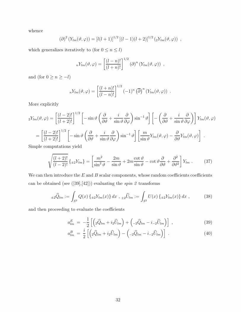
whence
(∂)2 (Ylm(ϑ, ϕ)) = [l(l + 1)]1/2 [(l − 1)(l + 2)]1/2 (2Ylm(ϑ, ϕ)) ,
which generalizes iteratively to (for 0 ≤ n ≤ l)
nYlm(ϑ, ϕ) =
[(l − n)!
(l + n)!
]1/2(∂)n (Ylm(ϑ, ϕ)) ,
and (for 0 ≥ n ≥ −l)
nYlm(ϑ, ϕ) =
[(l + n)!
(l − n)!
]1/2(−1)n
(∂)n
(Ylm(ϑ, ϕ)) .
More explicitly
2Ylm(ϑ, ϕ) =
[(l − 2)!
(l + 2)!
]1/2 [− sinϑ
(∂
∂ϑ+
i
sinϑ
∂
∂ϕ
)sin−1 ϑ
] [−
(∂
∂ϑ+
i
sin ϑ
∂
∂ϕ
)]Ylm(ϑ, ϕ)
=
[(l − 2)!
(l + 2)!
]1/2 [− sin ϑ
(∂
∂ϑ+
i
sinϑ
∂
∂ϕ
)sin−1 ϑ
] [m
sinϑYlm(ϑ, ϕ)−
∂
∂ϑYlm(ϑ, ϕ)
].
Simple computations yield
√(l + 2)!
(l − 2)!{±2Ylm} =
[m2
sin2 ϑ−
2m
sinϑ+ 2m
cotϑ
sin ϑ− cotϑ
∂
∂ϑ+
∂2
∂ϑ2
]Ylm . (37)
We can then introduce the E andB scalar components, whose random coefficients coefficients
can be obtained (see ([39],[42])) evaluating the spin 2 transforms
±2Qlm :=
∫
S2
Q(x) {±2Ylm(x)} dx , ±2Ulm :=
∫
S2
U(x) {±2Ylm(x)} dx , (38)
and then proceeding to evaluate the coefficients
aElm = −1
2
[(2Qlm + i2Ulm
)+(−2Qlm − i−2Ulm
)], (39)
aBlm =i
2
[(2Qlm + i2Ulm
)−
(−2Qlm − i−2Ulm
)]. (40)
32