Spin-entangled electrons in solid-state systems ∗

Guido Burkard

Department of Physics and Astronomy, University of Basel, Klingelbergstrasse 82,CH-4056 Basel, Switzerland

Entanglement is one of the fundamental resources for quantum information process-

ing. This is an overview on theoretical work focused on the physics of the detection,

production, and transport of entangled electron spins in solid-state structures.

Contents

I. Introduction 2

A. Entanglement 2

B. Electron spin entanglement 3

C. What is not covered by this review 4

II. Detection of spin entanglement 5

A. Localized electrons: Coupled quantum dots 5

B. Coupled dots with superconducting contacts 7

C. Mobile electrons: Beam splitter shot noise 8

D. Leads with many modes 14

E. Lower bounds for entanglement 17

F. Use of spin-orbit coupling 20

G. Backscattering 21

H. Bell’s inequalities 22

III. Production of spin entanglement 23

A. Superconductor-normal junctions 23

B. Superconductor-Luttinger liquid junctions 25

C. Quantum dots coupled to normal leads 27

∗ Published as: J. Phys.: Condens. Matter 19, 233202 (2007).

2

D. Coulomb scattering in a 2D electron system 27

E. Other spin entangler proposals 28

IV. Transport of Entangled Electrons 28

References 31

I. INTRODUCTION

A. Entanglement

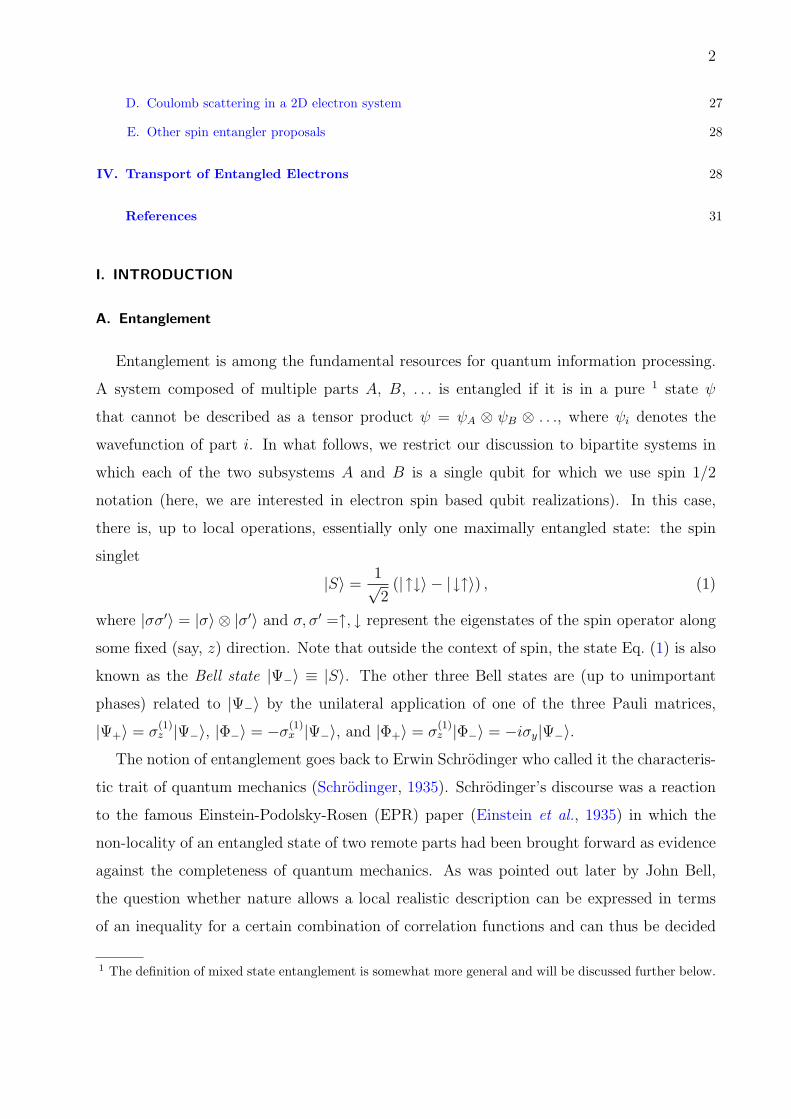
Entanglement is among the fundamental resources for quantum information processing.

A system composed of multiple parts A, B, . . . is entangled if it is in a pure 1 state ψ

that cannot be described as a tensor product ψ = ψA ⊗ ψB ⊗ . . ., where ψi denotes the

wavefunction of part i. In what follows, we restrict our discussion to bipartite systems in

which each of the two subsystems A and B is a single qubit for which we use spin 1/2

notation (here, we are interested in electron spin based qubit realizations). In this case,

there is, up to local operations, essentially only one maximally entangled state: the spin

singlet

|S〉 =1√2

(|↑↓〉 − |↓↑〉) , (1)

where |σσ′〉 = |σ〉 ⊗ |σ′〉 and σ, σ′ =↑, ↓ represent the eigenstates of the spin operator along

some fixed (say, z) direction. Note that outside the context of spin, the state Eq. (1) is also

known as the Bell state |Ψ−〉 ≡ |S〉. The other three Bell states are (up to unimportant

phases) related to |Ψ−〉 by the unilateral application of one of the three Pauli matrices,

|Ψ+〉 = σ(1)z |Ψ−〉, |Φ−〉 = −σ(1)

x |Ψ−〉, and |Φ+〉 = σ(1)z |Φ−〉 = −iσy|Ψ−〉.

The notion of entanglement goes back to Erwin Schrodinger who called it the characteris-

tic trait of quantum mechanics (Schrodinger, 1935). Schrodinger’s discourse was a reaction

to the famous Einstein-Podolsky-Rosen (EPR) paper (Einstein et al., 1935) in which the

non-locality of an entangled state of two remote parts had been brought forward as evidence

against the completeness of quantum mechanics. As was pointed out later by John Bell,

the question whether nature allows a local realistic description can be expressed in terms

of an inequality for a certain combination of correlation functions and can thus be decided

1 The definition of mixed state entanglement is somewhat more general and will be discussed further below.

3

experimentally if a source of entangled pairs (also called EPR pairs) like the one in Eq. (1)

is available (Bell, 1966; Mermin, 1993). Such experiments have been carried out using the

two linear polarizations of photons as the “qubit states” (Aspect et al., 1982), providing

strong evidence against local realism and for the completeness of quantum mechanics as a

description of nature.

The non-locality of a system in state Eq. (1) can be viewed as a limitation since it prohibits

any local description. However, from a quantum information point of view, entanglement

and non-locality are “features” rather than “bugs” of quantum mechanics. This is so because

entanglement between remote parties (A and B) in a quantum communications setting can

be used as a resource for a variety of quantum protocols (Bennett and DiVincenzo, 2000).

Among these are quantum teleportation, i.e., the faithful transmission of a quantum state

using a classical channel plus previously shared entanglement (Bennett et al., 1993), some

variants of quantum key distribution (Ekert, 1991), i.e., the generation of an unconditionally

secure cryptographic key using EPR pairs, and quantum dense coding (Bennett and Wiesner,

1992), i.e., the transmission of two classical bits by sending only one qubit and using one

EPR pair. This list is by no means exhaustive: given that quantum channels can also

be noisy, there exists an entire family of quantum protocols (Devetak et al., 2004). In

addition to the aforementioned experimental test of Bell’s inequalities (Aspect et al., 1982),

several quantum communication protocols have been realized experimentally with entangled

photons, among them dense coding (Mattle et al., 1996), quantum teleportation (Boschi

et al., 1998; Bouwmeester et al., 1997), and quantum cryptography (Gisin et al., 2002).

B. Electron spin entanglement

The electron spin is a natural two-level system which makes it an ideal candidate for

a solid-state qubit (Loss and DiVincenzo, 1998). Two electron spin qubits, each localized

in one of two adjacent semiconductor quantum dots, can be coupled via the Heisenberg

exchange interaction due to virtual electron tunneling between the quantum dots (Burkard

et al., 1999). Experimentally, there has been remarkable progress toward electron spin qubits

in structures such as quantum dots: The storage, preparation, coherent manipulation of a

single electron spin in a quantum dot and the controlled coupling of two spins located in

separate dots has been demonstrated experimentally (Hanson et al., 2006). This article is a

4

review of work dedicated to the question whether EPR pairs consisting of two electrons with

entangled spins could be used perform those quantum protocols and to test Bell’s inequalities

and in a solid-state system. Since the use of entangled electron spin pairs in solid-state

structures was theoretically proposed and analyzed (Burkard et al., 2000), there has been a

growing activity aimed at understanding physical mechanisms that generate spin-entangled

electrons in mesoscopic conductors. On the experimental side, electron spin entanglement,

the violation of Bell’s inequalities, or the realization of a quantum communication protocol

with electron spins in a solid have not been reported so far, but experiments are still under

way in this direction. One may also envision the conversion of spin entanglement of localized

(Gywat et al., 2002) or mobile (Cerletti et al., 2005) electrons an efficient and deterministic

means to generate polarization-entangled photons.

Entanglement is not uncommon in solid-state systems. On the contrary, entanglement is

the rule rather than the exception in the low-energy states (say, the ground state) of inter-

acting many-particle systems. However, such “generic” entangled states are not necessarily

useful for quantum information processing. A criterion for the usefulness as a resource is that

there must be a realizable physical mechanism to extract and separate a “standard” pair of

entangled particles such as the EPR pair in Eq. (1) from the many-body system in such a

way that the two particles can be used for quantum communication. This is often compli-

cated by the indistinguishability of the particles: in this case, a state that “looks entangled”

when written out in first quantized notation might not be entangled in an operational sense

(i.e., there may not be any physical procedure that separates the particle while maintaining

their entanglement). Mathematically, this is related to the fact that the Hilbert space for

several identical particles is not a tensor product when proper antisymetrization is taken

into account. Measures of entanglement which take into account the indistinguishability of

particles have been introduced (Dowling et al., 2006; Schliemann et al., 2001a,b; Wiseman

and Vaccaro, 2003).

C. What is not covered by this review

This article is about spin entanglement between two electrons in solid-state structures.

It does not cover orbital entanglement of charge carriers, such as electron-hole entanglement

(see (Beenakker, 2006)), (orbital) exciton entanglement (Hohenester, 2002), orbital entangle-

5

ment between electrons (Samuelsson et al., 2003), and entanglement between encoded spin

states (Taylor et al., 2005). Another review on some of the topics covered here is (Egues

et al., 2003).

II. DETECTION OF SPIN ENTANGLEMENT

What physically measurable consequences does the entanglement of two electron spins

in an entangled state like Eq. (1) have? How can one tell an entangled pair of electron

spins (or a stream thereof) from an unentangled one? We will describe several tests for

spin entanglement in this section. One of the most straight-forward methods would be to

test Bell’s inequality directly (in fact, such proposals have been made for electron spins

in solids, as we will briefly report in Sec. II.H, further below). However, testing Bell’s

inequality involves measuring single electron spins one by one along at least three non-

collinear quantization axes, which is by no means a simple practical task.

There is an alternative to direct Bell tests which allows to gain information about spin

entanglement from a charge measurement by exploiting the Fermi statistics of the electrons,

giving rise to a unique relation between the symmetry of the orbital state and the two-

electron spin state. Such charge measurements can be of two different types: electrostatic

(via a nearby quantum point contact or single-electron transistor) or transport (measure-

ments of the current and/or its fluctuations).

A. Localized electrons: Coupled quantum dots

We first consider a setup that can be used to probe the entanglement of two electrons

localized in a double-dot (as shown in Fig. 1) by measuring a transport current and its

fluctuations, or current noise (Loss and Sukhorukov, 2000). The parameter regime of interest

is that of weak coupling between the double dot and the in- and outgoing leads (which

are held at the chemical potentials µ1, 2) with tunneling amplitude T , where the dots are

shunted in parallel. Moreover, the parameters need to lie in (i) the Coulomb blockade regime

(Kouwenhoven et al., 1997) where the charge on the dots is quantized and (ii) the cotunneling

regime (Averin and Nazarov, 1992), where single-electron tunneling is suppressed by energy

conservation. The cotunneling regime is defined by U > |µ1±µ2| > J > kBT, 2πνT 2 with U

6

FIG. 1 Setup for detecting entanglement of two localized electrons in two tunnel-coupled quantum

dots (Loss and Sukhorukov, 2000). Each dot is filled with one electron and is coupled via a tunneling

amplitude T to each of the two leads. In addition, the two quantum dots are tunnel-coupled

amongst each other, which leads to an inter-dot exchange coupling J , energetically favoring the

entangled singlet state to the triplet states of the two spins. For the detection of this entanglement,

the current and/or current fluctuations from lead 1 to lead 2 need to be observed as a function of

the magnetic flux Φ threading the loop enclosed by the tunneling paths.

the charging energy on a single-dot, ν the density of states in the leads, and J the exchange

coupling between the spins on the two dots. The electric current in the cotunneling regime

is generated by a coherent virtual process where one electron tunnels from one of the dots

to one of the leads (say, lead 2) and then a second electron tunnels from the other lead (in

our example, lead 1) to the same dot. For bias voltages exceeding the exchange coupling,

|µ1 − µ2| > J , both elastic and inelastic cotunneling are permitted. It is assumed that T

is sufficiently small for the double-dot system to equilibrate after each tunneling event. An

electron can either pass through the upper or through the lower dot, such that a closed

loop is formed by these two paths. An externally applied magnetic field B then induces a

magnetic flux Φ = AB that threads this loop (with area A) and leads to an Aharonov-Bohm

(AB) phase φ = eΦ/~ between the upper and the lower path. The AB phase influences the

quantum interference between the two paths. Such a transport setting is sensitive to the

spin symmetry of the two-electron state on the double dot; if the two electrons on the

double-dot are in the singlet state |S〉, as in Eq. (1), then the tunneling current acquires an

additional phase of π leading to a sign reversal of the coherent contribution compared to

7

that for triplets,

|T−1〉 = |↓↓〉 =1√2

(|Φ+〉 − |Φ−〉) , (2)

|T0〉 =1√2

(|↑↓〉+ |↓↑〉) = |Ψ+〉, (3)

|T+1〉 = |↑↑〉 =1√2

(|Φ+〉+ |Φ−〉) . (4)

This phase is reflected in the sign of an interference term in the average current in the

cotunneling regime (Loss and Sukhorukov, 2000)

I = eπν2T 4 µ1 − µ2

µ1µ2

(2± cosφ) , (5)

where the upper (lower) sign belongs to the triplet (singlet) states in the double-dot. The

fluctuations of the electric current (shot noise) follow Poissonian statistics with noise power

S(0) = −e|I|, and thus they inherit the dependence on the spin state from that of the

average current. Note that the singlet is maximally entangled (see above) while one of the

triplets (|T0〉) is entangled (hence, |T0〉 is also an EPR pair) and the other two (|T±〉) are

not entangled. Therefore, if the singlet can be distinguished from the triplet, then at least

for one outcome (singlet), entanglement has been detected unambiguously.

For finite frequencies the shot noise is proportional to the same statistical factor (Loss

and DiVincenzo, 1998), S(ω) ∝ (2 ± cosφ), where the odd part of S(ω) leads to slowly

decaying oscillations of the noise in real time, S(t) ∝ sin(µt)/µt, µ = (µ1 + µ2)/2. This

decay is due to a charge imbalance between the two dots during a time ∆t ≈ µ−1. A general

study of the quantum shot noise in cotunneling through coupled quantum dot systems can

be found in (Sukhorukov et al., 2001).

B. Coupled dots with superconducting contacts

A setup similar to the one shown in Fig. 1 with two quantum dots, but connected to su-

perconducting (SC) leads (with tunneling amplitude T ), and without direct tunnel-coupling

between the dots, has been considered in (Choi et al., 2000). This setup is shown in Fig. 2.

Two main results have been reported for this system: The coupling to the SC leads (i)

energetically favors an entangled singlet-state on the dots, and (ii) provides a mechanism

for detecting the spin state via the Josephson current through the double dot system.

8

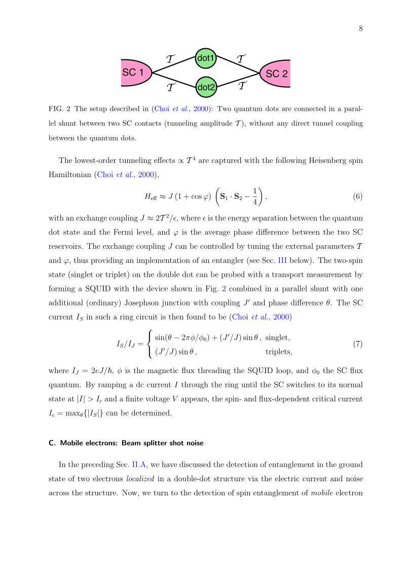
FIG. 2 The setup described in (Choi et al., 2000): Two quantum dots are connected in a paral-

lel shunt between two SC contacts (tunneling amplitude T ), without any direct tunnel coupling

between the quantum dots.

The lowest-order tunneling effects ∝ T 4 are captured with the following Heisenberg spin

Hamiltonian (Choi et al., 2000),

Heff ≈ J (1 + cosϕ)

(S1 · S2 −

1

4

), (6)

with an exchange coupling J ≈ 2T 2/ε, where ε is the energy separation between the quantum

dot state and the Fermi level, and ϕ is the average phase difference between the two SC

reservoirs. The exchange coupling J can be controlled by tuning the external parameters T

and ϕ, thus providing an implementation of an entangler (see Sec. III below). The two-spin

state (singlet or triplet) on the double dot can be probed with a transport measurement by

forming a SQUID with the device shown in Fig. 2 combined in a parallel shunt with one

additional (ordinary) Josephson junction with coupling J ′ and phase difference θ. The SC

current IS in such a ring circuit is then found to be (Choi et al., 2000)

IS/IJ =

sin(θ − 2πφ/φ0) + (J ′/J) sin θ , singlet,

(J ′/J) sin θ , triplets,(7)

where IJ = 2eJ/~, φ is the magnetic flux threading the SQUID loop, and φ0 the SC flux

quantum. By ramping a dc current I through the ring until the SC switches to its normal

state at |I| > Ic and a finite voltage V appears, the spin- and flux-dependent critical current

Ic = maxθ{|IS|} can be determined.

C. Mobile electrons: Beam splitter shot noise

In the preceding Sec. II.A, we have discussed the detection of entanglement in the ground

state of two electrons localized in a double-dot structure via the electric current and noise

across the structure. Now, we turn to the detection of spin entanglement of mobile electron

9

FIG. 3 The beam-splitter setup. An entangler (see Sec. III) transforms uncorrelated electrons

(here schematically indicated as leads 1′ and 2′) into pairs of electrons in the entangled singlet

(triplet) state |Ψ∓〉, which are injected into leads 1, 2 (one electron per lead). The entanglement

of the spin singlet can then be detected in an interference measurement with the beam splitter:

Since the orbital wave function of the singlet is symmetric, the electrons leave the scattering region

preferably in the same lead (3 or 4), cf. Table I. This correlation of the particle number (“bunching”)

manifests itself in an enhancement of the shot noise by a factor of 2 in the outgoing leads.

spins. For this purpose, the electron pair to be tested will itself carry the electric current. It

turns out that pairwise spin entanglement between electrons in two mesoscopic conductors

can be detected in the fluctuations of the charge current after transmission through an

electronic beam splitter (Burkard et al., 2000) as shown schematically in Fig. 3. As we discuss

in detail below, the singlet EPR pair Eq. (1) produces an enhancement of the shot noise

power (“bunching” behavior), whereas the triplets |T0,±1〉, Eqs. (2–4) lead to a suppression

of noise (“antibunching”).

This result can be understood by inspection of Table I. For indistinguishable, Fermionic

particles such as electrons, the antisymmetry of the total wavefunction (spin and orbit

combined) dictates that the orbital wavefunction must be symmetric if the spin wavefunction

is antisymmetric (as in the case of the spin singlet) and vice versa for the triplets. Assuming

state spin wavefunction orbital wavefunction final states (orbit) 〈δN23 〉 entanglement

|S〉 antisymmetric symmetric |33〉, |44〉 1 yes

|T0〉 symmetric antisymmetric |34〉 − |43〉 0 yes

|T±〉 symmetric antisymmetric |34〉 − |43〉 0 no

distinguishable — — |33〉, |44〉, |34〉, |43〉 1/2 possible

TABLE I Number statistics for Fermions at a symmetric beam splitter.

10

that each conductor has only one channel (which we simply denote |n〉 where n is the label of

the contact), we can easily enumerate all possible final states with the prescribed symmetry.

The task of the beam splitter is to distribute the particles over these possible states in order

to probe the symmetry properties of the wavefunction. For a symmetric beam splitter where

the transmission and reflection probabilities are both 1/2 (for the general case, see below),

each of these states allowed by symmetry is filled with equal probability. Then, it is easy

to obtain the mean and variance of the probability distribution for N = N3, the number of

outgoing electrons in lead n = 3 (Loudon, 1998). The mean is always 〈N〉 = 1 and does not

contain any information on the statistics or entanglement of the ingoing state. We therefore

do not expect that here (unlike for the localized electrons in Sec. II.A), the average electric

current will contain any information about the spin state. However, the variance 〈δN23 〉

vanishes for triplets because there is only one possible final state and thus fluctuations

are impossible (this behavior is called “antibunching” of particles), while for the singlet

〈δN23 〉 = 1 which is twice as large as expected for (classical) distinguishable particles (also

known as “bunching”). Note that for Bosons (e.g., photons), since the total wavefunction

must be symmetric, the role of singlet and triplet are interchanged. In fact, for Bosons, this

effect is well known as the Hong-Ou-Mandel dip in interferometry with entangled photon

pairs (Hong et al., 1987). Bunching behavior for (unentangled) Bosons also underlies the

famous Hanbury-Brown and Twiss experiment (Hanbury Brown and Twiss, 1956).

Here, we are interested in the fact that particle bunching, i.e., the enhancement of the

fluctuations of the electron current, is only possible for an entangled state (the singlet) and

thus particle bunching is a unique signature for entanglement. Nothing of this sort can

be said for antibunching, since there are both entangled and unentangled triplets. This

result can be extended to non-maximally entangled states (see below for a quantitative

discussion); we only anticipate here that in Table I, we find 〈δN23 〉 ≤ 1/2 for all unentangled

states. Conversely, a number fluctuation 〈δN23 〉 > 1/2 can be interpreted as a signature of

entanglement. However, we still need to relate 〈δN23 〉 to a physically measurable quantity

(the shot noise power at low frequencies).

Let us now turn to the physical setup (Fig. 3) with a beam splitter where electrons

have an amplitude t to be interchanged (without mutual interaction) such that 0 < |t|2 <

1. Shot noise of the electric current in such beam splitter devices have been studied for

normal (unentangled) electrons both in theory (Buttiker, 1990, 1992; Martin and Landauer,

11

1992; Torres and Martin, 1999) and experiment (Henny et al., 1999; Liu et al., 1998; Oliver

et al., 1999). Recent experiments have investigated the sign of the cross-correlations after

transmission of fermions through a beam splitter and the distinction between the effects from

Fermi statistics and other effects such as noisy injection and interactions (Chen and Webb,

2006; Oberholzer et al., 2006). These experiments have been performed in semiconductor

nanostructures with geometries that are very similar to the set-up proposed in Fig. 3 but

without any entangler device.

The effect of interactions in the leads will be addressed in Sec. IV below. To calculate

the shot noise of spin-entangled electrons, standard scattering theory (Blanter and Buttiker,

2000; Buttiker, 1990, 1992), was extended to a situation with entanglement (Burkard et al.,

2000). The entangled two-electron state injected into two distinct leads 1 and 2 can be

written in second quantized notation as

|Ψ±〉 ≡ |ψt/snn′〉 =

1√2

(a†n↑a†n′↓ ± a†n↓ a

†n′↑ ) |ψ0〉, (8)

where s and t stand for the singlet and triplet, |ψ0〉 for the filled Fermi sea, and n =

(q, l), where q denotes the momentum and l the lead quantum number of an electron.

The operator a†nσ creates an electron in state n with spin σ. Alternatively, we can use

the quantum numbers n = (εn, n), with the electron energy εn instead of the momentum

as the orbital quantum number in Eq. (8). The operator a†ασ(ε) then creates an incoming

electron in lead α with spin σ and energy ε. After being injected, the two electrons are no

longer distinguishable from the electrons that had been in the leads before, and consequently

the two electrons retrieved from the system will, in general, not be “the same” as the

ones injected. When extending the theory for the current correlations in a multiterminal

conductor (Buttiker, 1990, 1992) to the case of entangled scattering states, we need to take

into account that Wick’s theorem cannot be applied anymore. The current operator for lead

α of a multiterminal conductor is

Iα(t) =e

hν

∑εε′σ

[a†ασ(ε)aασ(ε′)− b†ασ(ε)bασ(ε′)

]exp [i(ε− ε′)t/~], (9)

with the operators bασ(ε) for the outgoing electrons, that are related to the operators

aασ(ε) for the incident electrons via bασ(ε) =∑

β sαβaβσ(ε), where sαβ is the scattering

matrix. Here, the scattering matrix is assumed to be spin- and energy-independent. For

a discrete energy spectrum in the leads, the operators aασ(ε) can be normalized such that

12

{aασ(ε), a†βσ′(ε′)} = δσσ′δαβδεε′/ν, where the Kronecker symbol δεε′ equals 1 if ε = ε′ and 0

otherwise and where ν denotes the density of states in the leads. As mentioned before, we

assume for the moment that each lead consists of only a single quantum channel, a more

general treatment will be discussed in Sec. II.D below. The current operator Eq. (9) can

now be written in terms of the scattering matrix as

Iα(t) =e

hν

∑εε′σ

∑βγ

a†βσ(ε)Aαβγaγσ(ε′)ei(ε−ε′)t/~, (10)

Aαβγ = δαβδαγ − s∗αβsαγ. (11)

The current-current correlator between Iα(t) and Iβ(t) in two leads α, β = 1, .., 4 of the

beam splitter is then

Sχαβ(ω) = lim

τ→∞

hν

τ

∫ τ

0

dt eiωt Re Tr [δIα(t)δIβ(0)χ] , (12)

where δIα = Iα − 〈Iα〉, 〈Iα〉 = Tr(Iαχ) and χ is the density matrix of the injected electron

pair. Here, we are interested in the zero-frequency correlator Sαβ ≡ Sχαβ(0). In order not

to overburden our notation, we omit the dependence on χ in what follows. If we substitute

χ = |Ψ±〉〈Ψ±| we obtain

Sαβ =e2

hν

[ ∑γδ

′Aα

γδAβδγ ∓ δε1,ε2

(Aα

12Aβ21+A

α21A

β12

)], (13)

where∑′

γδ denotes the sum over γ = 1, 2 and all δ 6= γ, and the upper (lower) sign refers

again to triplets (singlets). Physically, the autocorrelator Sαα is the shot noise measured in

lead α.

The formula Eq. (13) can now be applied to the setting shown in Fig. 3, i.e., involving

four leads and described by the single-particle scattering matrix elements, s31 = s42 = r,

and s41 = s32 = t, where r and t denote the reflection and transmission amplitudes at the

beam splitter. If we neglect backscattering (see Sec. II.G for a discussion of the influence of

backscattering), i.e., s12 = s34 = sαα = 0, then the noise correlations for the incident state

|Ψ±〉 are found to be (Burkard et al., 2000)

S33 = S44 = −S34 = 2e2

hνT (1− T ) (1∓ δε1ε2) , (14)

with T = |t|2 the transmittivity of the beam splitter. One can check that for the remaining

two triplet states |↑↑〉 and |↓↓〉 one also obtains Eq. (14) with the upper sign. As anticipated,

13

the average current in all leads is a constant, both for singlets and triplets, |〈Iα〉| = e/hν. The

shot noise power is often expressed in terms of the noise-to-current ratio (or, more accurately,

the ratio between the actual noise power and that of a Poissonian source (Blanter and

Buttiker, 2000)), the so-called Fano factor, F = Sαα/2e |〈Iα〉|. In our case, the theoretical

prediction for the Fano factor is (note the absence of a factor of 2e with the above definition

of the Fano factor),

F = T (1− T ) (1∓ δε1ε2) . (15)

The formula Eq. (15) implies that if electrons in the singlet state |Ψ−〉 with equal energies,

ε1 = ε2, i.e., in the same orbital mode, are injected pairwise into the leads 1 and 2, then the

zero frequency noise is enhanced by a factor of two (Burkard et al., 2000), F = 2T (1−T ), with

respect to the noise power for unentangled (uncorrelated) electrons (Buttiker, 1990, 1992;

Khlus, 1987; Landauer, 1989; Lesovik, 1989; Martin and Landauer, 1992), F = T (1 − T ).

As explained above, this noise enhancement is due to bunching of electrons in the outgoing

leads, caused by the symmetric orbital wavefunction of the spin singlet |S〉 = |Ψ−〉. The

triplet states |T0〉 = |Ψ+〉, | ↑↑〉, and | ↓↓〉 exhibit antibunching, i.e. a complete suppression

of the noise, Sαα = 0. The noise enhancement for the singlet |Ψ−〉 is therefore a unique

signature for entanglement (no unentangled state exists which can lead to the same signal).

Entanglement can thus be observed by measuring the noise power of a mesoscopic conductor

in a setup like Fig. 3. Distinguishing the triplet states |Ψ+〉, | ↑↑〉, and | ↓↓〉 is not possible

with the described noise measurement alone; their discrimination requires a measurement

of the spins of the outgoing electrons, e.g. by using spin-selective tunneling devices (Prinz,

1998) into leads 3 and 4. However, as we shall discuss in Sec. II.F below, there are ways

to detect triplet entanglement if a local spin rotation mechanism (e.g., provided by the

spin-orbit interaction) is available in at least one of the ingoing leads.

Signatures of entanglement in the charge transport statistics have also been formulated

in the framework of the full counting statistics (Borlin et al., 2002; Di Lorenzo and Nazarov,

2005; Faoro et al., 2004; Taddei et al., 2005; Taddei and Fazio, 2002). The generalization

(for both Bosons and Fermions) to many particles interfering at a multi-port beam splitter

is discussed in (Lim and Beige, 2005).

14

D. Leads with many modes

In our discussion so far, we have assumed that the leads that carry the spin-entangled

electrons from the entangler to the beam splitter only conduct electrons via a single quantized

mode. This has been extended to the continuum limit for the lead spectrum in (Samuelsson

et al., 2004). We will follow a somewhat more general discussion (including the continuum

case) for leads with multiple modes as presented in (Egues et al., 2005). In this general

discussion, the parameter regimes in which singlet spin entanglement can be detected in

the shot noise at a beam splitter (as discussed in Sec. II.C above) have been identified. It

turns out that even in the case where the entangled electrons are injected into a multitude of

discrete states of the lead, we can observe two-particle coherence, and thus particle bunching

and antibunching, and thus detect entangled states. In our discussion, we are not considering

the possibility that in a multi-mode setting, the two injected electrons can also be entangled

in their orbital degrees of freedom. This possibility and its consequences for the entanglement

detection via a noise measurement at a beam splitter has been investigated in (Giovannetti

et al., 2006).

For our purposes, we first identify the relevant energy scales for the transport through

multiple modes. These are the level spacing δ in the leads, the energy mismatch ∆ of

the injected electrons, and the energy broadening γ of the injected electrons (see Fig. 4).

The relative magnitude of these three energies determine six different parameter regimes.

In four of the six regimes, the full two-particle interference (and thus detection of spin

entanglement) can be achieved asymptotically. In the two remaining parameter regimes,

characterized by ∆ � δ, γ, i.e., the energy mismatch exceeding both the level spacing and

the energy broadening, we obtain no two-particle interference (these represent two distinct

parameter regimes, since δ can be smaller or larger than γ).

The lead spectrum is assumed to consist of equidistant levels, i.e., εn = nδ + qδ, where

n = 0,±1,±2, . . . and 0 ≤ q < 1 is some fixed offset. The injection of an electron with spin

σ =↑, ↓ into the lead α with energy distribution g(ε, εn) centered at εn is now described by

the creation operator

c†ασ(ε) =∞∑

n=−∞

g(ε, εn)a†ασ(εn), (16)

where a†ασ(εn) creates an electron with the sharp energy εn as in Eq. (8). For the weight

15

g( , )g( , )

δq.

ε2

ε2 εεε1

...

ε1∆

δ

0

1

2

−1

−2

n

...

3γ

FIG. 4 Energy diagram for the injection of entangled electrons into leads with multiple levels

(Egues et al., 2005). In the model discussed in the main text, the energy levels in the leads

n = 0,±1,±2, . . . are assumed to be equidistant with spacing δ. The injection of electrons takes

place at the mean energies ε1,2 (for electron 1 and 2, respectively), separated by ∆ = ε2 − ε1, and

with distributions g(ε1,2, ε) of width γ. Here, the distributions g(ε1,2, ε) are not drawn to scale,

since their normalizations depend on the value of q.

function g, we use the Breit-Wigner form

g(ε, ε′) =g0(ε)

ε− ε′ + iγ, (17)

subject to the normalization condition∑∞

n=−∞ |g(ε, ε′)|2 = 1.

Here, we assume that the entangler injects an electron with total probability 1, but with

uncertain energy (e.g., using time-dependent tunnel barriers). This is different form the

weak tunneling case, e.g., from a quantum dot (Recher et al., 2001). Analogous to Eq. (8),

the spin-entangled singlet (−) and triplet (+) states for many-mode leads can be written

with the new creation operators as

|Ψ±〉 =1√2

(c†1↑(ε1)c

†2↓(ε2)± c†1↓(ε1)c

†2↑(ε2)

)|ψ0〉. (18)

The relation Eq. (16) allows us to express these states as

|Ψ±〉 =∑ε′1,ε′2

g(ε1, ε′1)g(ε2, ε

′2)|Ψ±〉ε′1,ε′2

, (19)

where |Ψ±〉ε′1,ε′2are the states with sharp energies, defined in Eq. (8). The normalization

condition for g(ε1, ε′1) ensures that the average current in the outgoing leads of the beam

16

splitter is unaffected by the spread in energy, i.e., I3 = I4 = −e/hν. However, the Fano

factor F = S33/2eI3 does depend on the energy distribution,

F = T (1− T )(1∓ |h(ε1, ε2)|2

), (20)

where the upper (lower) sign corresponds to the entangled triplet (singlet), and where the

overlap function h is defined as

h(ε1, ε2) =∑

ε

g(ε2, ε)∗g(ε1, ε). (21)

For equidistant levels, this function has been evaluated exactly (note that the q dependence

has dropped out),

|h|2 =γ2

(∆/2)2 + γ2

cosh2(2πγ/δ)− cos2(π∆/δ)

sinh2(2πγ/δ). (22)

In the case of injection into a single level, the |h|2 term that appears in Eq. (20) for

the Fano factor reduces to a Kronecker delta, as in Eq. (15). The role of the function

0 < |h(∆, δ, γ)|2 ≤ 1 is to quantify the visibility of two-particle interference. We plot the

dimensionless quantity |h(∆, δ, γ)|2 as a function of the dimensionless ratios ∆/δ and δ/γ

in Fig. 5. For maximal visibility, |h|2 = 1, full bunching and antibunching of singlets and

entangled triplets can be expected; this is the ideal case with regards to the detection of

entanglement. In the opposite case |h|2 = 0, bunching or antibunching cannot be observed

at all because the two wave packets centered around ε1 and ε2 do not overlap in energy.

We briefly highlight the main parameter regimes (see also Fig. 5). (1) If the two electrons

are injected with energy distributions whose centers coincide, ∆ = ε1 − ε2 = 0, then the

interference is always maximal, |h|2 = 1, irrespective of the values of the parameters δ and

γ. For finite but small ∆, i.e., ∆ � γ, δ, one finds |h|2 = 1 − O(∆2). More precisely, for

∆ � γ � δ, the correction is |h|2 ' 1 − π2∆2/3δ2, whereas for ∆ � δ � γ, one finds

|h|2 ' 1−∆2/4γ2. (2) If the energy broadening is small, γ � δ,∆, then Eq. (22) yields

|h|2 =δ2

π2∆2sin2 π

∆

δ+O(γ2). (23)

Here, the ratio δ/∆ is essential: If γ � δ � ∆ then the two electrons are injected into two

different discrete states, therefore |h|2 → 0. In the opposite limit, γ � ∆ � δ, the two

electrons are injected into the same discrete level and |h|2 = 1− π2∆2/3δ2 + O(∆4/δ4, γ2).

17

|h| 2

02

4

1

0 δ/γ4

2

0

∆/δ

δ

δ

small

∆

large γ

large

small

FIG. 5 The two-particle interference visibility |h(∆, δ, γ)|2 from Eq. (22), plotted as a function of

the dimensionless quantities ∆/δ and δ/γ, where ∆ = ε2 − ε1 denotes the mean energy difference

between the two injected electrons, γ the width of their energy distributions, and δ the level spacing

in the leads (see Fig. 4). The special case of matching energies ε1 ≈ ε2 or ∆ � δ, γ corresponds

to the edge labeled by “small ∆”; here we find |h|2 = 1, irrespective of the ratio γ/δ. The case

of a broad energy distribution (fast injection) γ � ∆, δ corresponds to the edge labeled “large γ”;

along this edge |h|2 = 1, regardless of ∆/δ. A line of constant γ and ∆ with variable δ is indicated

by a red arrow. For large δ, we find again |h|2 = 1 for all ∆/γ, whereas for small δ (continuum

limit), the limit |h|2 = 0 or |h|2 = 1 is reached, depending on whether ∆/γ � 1 or ∆/γ � 1.

(3) The continuum limit is reached when δ � ∆, γ. In this case |h|2 has the shape of a

Lorentzian (Samuelsson et al., 2004),

|h|2 ' γ2

(∆/2)2 + γ2. (24)

Depending on the ratio γ/∆, the two-particle interference is present or absent, i.e., |h|2 → 0

for δ � γ � ∆, while |h|2 → 1 for δ � ∆ � γ. In summary, highly visible two-

particle interference (and thus bunching and antibunching) |h|2 → 1 can be expected in all

asymptotic regimes except for the detuned cases, ∆ � δ, γ, where |h|2 → 0.

E. Lower bounds for entanglement

In Sec. II.C above, the current fluctuations for a maximally entangled state (the singlet)

has been discussed. Here, we extend this analysis to non-maximally entangled states. Such

18

states can be both pure or mixed, and therefore are generally described by a density matrix

χ. It turns out (Burkard and Loss, 2003) that using the zero-frequency noise amplitude

after passage through the beam splitter (Fig. 6), one can determine a lower bound for the

amount E of spin entanglement carried by individual pairs of electrons. One can therefore

relate experimentally accessible quantities with a standard measure for entanglement, the

entanglement of formation E (Bennett et al., 1996b). Such knowledge is important since E

quantifies the usefulness of a bipartite state for quantum communication.

We start our discussion from a general mixed state which we write in the singlet-triplet

basis,

χ = FS|Ψ−〉〈Ψ−|+G0|Ψ+〉〈Ψ+|+∑i=↑,↓

Gi|ii〉〈ii|+ ∆χ, (25)

where ∆χ denote off-diagonal terms. The singlet fidelity FS quantifies the probability that

the electron pair is in a spin singlet state (we use the subscript S here in order to distinguish

the singlet fidelity from the Fano factor; in the literature, F is often used for FS). Next, one

can decompose the current correlators Eq. (12) as

Sαβ ≡ Sχαβ = FSS

|Ψ−〉αβ +G0S

|Ψ+〉αβ +

∑i=↑,↓

GiS|ii〉αβ , (26)

where we have defined S|Ψ〉αβ ≡ S

|Ψ〉〈Ψ|αβ . The off-diagonal terms in ∆χ need not be specified

further, as they do not enter Sαβ due to the spin-conserving nature of the operators δIα(t).

The prefactors FS, G0, G↑, and G↓ are the diagonal matrix elements of χ and are determined

by the state preparation, i.e., the entangler.

In Sec. II.C we showed that the singlet state |S〉 = |Ψ−〉 gives rise to enhanced shot noise

(and cross-correlators), S|Ψ−〉33 = −S|Ψ−〉

34 = 2eIT (1− T )f , with the reduced correlator f = 2,

as compared to the “classical” Poissonian value f = 1. The spin triplet states, on the other

hand, are noiseless, S|Ψ+〉αβ = S

|↑↑〉αβ = S

|↓↓〉αβ = 0 (α, β = 3, 4). Therefore, both the auto- and

cross-correlations are only due to the singlet component of the incident two-particle state,

S33 = −S34 = FSS|Ψ−〉 = 2eIT (1− T )f, (27)

where f = 2FS. So, a noise measurement simply provides us with the information about the

singlet fraction of the state. This already suggests that in general, we cannot expect to get

full information about the entanglement E of the state, since E is a function of the entire

density matrix χ of which we know only one matrix element! From this point of view it is

19

astonishing how much we can know about the entanglement E by knowing only FS: as we

explain below, we can always obtain a lower bound on E which becomes tight if the state is

a singlet (FS = 1, E = 1) or any other spherically symmetric state.

Given a pure bipartite state, |ψ〉 ∈ HA ⊗ HB, we can use the von Neumann entropy

SN(|ψ〉) = −TrBρB log ρB (log in base 2) of the reduced density matrix ρB = TrA|ψ〉〈ψ|,

to quantify the entanglement. This quantity is always between 0 and 1, 0 ≤ SN ≤ 1, and

is maximal for the Bell states, SN(|Ψ±〉) = SN(|Φ±〉) = 1. If it vanishes, then the state

is unentangled (i.e., a tensor product state), SN(|ψ〉) = 0 ⇔ |ψ〉 = |ψ〉A ⊗ |ψ〉B. The

operational meaning is that if SN(|ψ〉) ' N/M then M ≥ N copies of |ψ〉 are sufficient to

perform, e.g., quantum teleportation of N qubits for N,M � 1 (and similarly for other

quantum communication protocols). Entanglement measures also exist for mixed states.

The entanglement of formation of a bipartite state χ (Bennett et al., 1996b) is defined

E(χ) = min{(|χi〉,pi)}∈E(χ)

∑i piSN(|χi〉), where E(χ) = {(|χi〉, pi)|

∑i pi|χi〉〈χi| = χ} is the

set of possible decompositions of the density matrix into ensembles of pure states. Therefore,

E is the smallest averaged entanglement of any ensemble of pure states realizing χ. In an

operational sense, E(χ) measures the number of EPR pairs (asymptotically, averaged over

many copies) required to form one copy of the state χ. A state with E > 0 is entangled (a

state with E = 1) is maximally entangled and thus pure), and neither local operations nor

classical communication (LOCC) between A and B can increase E.

Given an arbitrary mixed state of two qubits χ, it is known that E(χ) is a relatively

complicated function of χ (Wootters, 1998). In particular, it is in general certainly not

a function of the singlet fidelity FS = 〈Ψ−|χ|Ψ−〉 alone. For the subclass of spherically

symmetric states, however, the entanglement only depends on FS, i.e., E(χ) = E(FS).

These states, known as Werner states (Werner, 1989), have the form

ρF = FS|Ψ−〉〈Ψ−|+1− FS

3(|Ψ+〉〈Ψ+|+ |Φ−〉〈Φ−|+ |Φ+〉〈Φ+|) . (28)

There is an explicit analytic expression for the entanglement of formation of the Werner

states (Bennett et al., 1996b):

E(FS) ≡ E(ρFS) =

H2

(1/2 +

√FS(1− FS)

)if 1/2 < FS ≤ 1,

0 if 0 ≤ FS < 1/2,(29)

where we have used the dyadic Shannon entropy H2(x) = −x log x − (1 − x) log(1 − x).

20

0 0.5 1F

0

1

E

0 1 2f

E

f

FS

FIG. 6 Entanglement of formation E of

the electron spins as a function of the sin-

glet fidelity FS and the reduced correlator

f = S33/2eIT (1 − T ) = 2FS . The points

on the curve represent the exact relation

for Werner states, the shaded (blue) area

above the curve represents general states,

for which the curve is a lower bound of E.

Possible values of E and f (or FS) are in

the shaded (blue) region.

Combining Eq. (29) with Eq. (27), one can express E(ρFS) in terms of the (reduced) shot

noise power f . The relation between E(ρFS) and FS (resp., f) is plotted in Fig. 6.

Using the expression for the entanglement of formation of Werner states, we can derive a

lower bound on the entanglement of arbitrary mixed states χ with the following argument.

An arbitrary mixed state χ can be transformed into a spherical symmetric state ρFSwith

FS = 〈Ψ−|χ|Ψ−〉 by a random bipartite rotation (“twirl”) (Bennett et al., 1996a,b), i.e. by

applying U ⊗ U with a random U ∈ SU(2). Because the twirl is a local (LOCC) operation,

entanglement can only decrease (or remain constant) under the twirl,

E(FS) ≤ E(χ). (30)

As a consequence, the entanglement of formation E(FS) of the associated Werner state (with

same singlet fidelity FS) is a lower bound on E(χ) (Fig. 6). If the noise power exceeds a

certain value, f = 2FS > 1, in the beam splitter setup Fig. 3 then we know that it must be

due to entanglement between the electron spins injected into leads 1 and 2, i.e., E(FS) > 0.

F. Use of spin-orbit coupling

The lower bound from Sec. II.E is useful if one is assessing a source that produces spin

singlet entanglement. An extension to arbitrary entangled states is possible if a means of

rotating the spin of the carriers in one of the ingoing arms of the beam splitter is available

(Burkard and Loss, 2003; Egues et al., 2002).

21

It has been proposed to use the Rashba spin orbit coupling in order to implement such

single-spin rotations in one of the leads going into the beam splitter (Egues et al., 2002).

This analysis has been extended to up to two bands with both Rashba and Dresselhaus

spin-orbit coupling present (Egues et al., 2005).

We restrict ourselves here to the Rashba spin-orbit coupling and a single mode of the

lead, to make the discussion as simple as possible. The Rashba spin-orbit coupling in, say,

lead 1, has the effect of rotating the spin injected in lead 1 by some angle θR. This can be

taken into account by multiplying the rotation matrix

UR =

cos θR/2 − sin θR/2

sin θR/2 cos θR/2

(31)

from the right to the scattering matrix blocks that involve lead 1, sR31 = s31UR and sR

41 =

s41UR. This rotates within the (entangled) singlet-triplet space, and yields the Fano factor

F = T (1− T )(1∓ cos θRδεε′), (32)

thus the classical inequality (F ≤ 1) can be violated for both the singlet and the entangled

triplet by sweeping the Rashba angle θR, while all unentangled triplet states still yield

F ≤ 1. Therefore, the Rashba rotation allows for the detection of entangled triplets in

addition to the singlet. Similarly, spin rotations about an arbitrary axis allow the detection

of all entangled states (in particular, all Bell states) with noise measurements.

G. Backscattering

Imperfections in the leads and the beam splitter can lead to undesired scattering of

electrons back into the same lead, or, e.g., from lead 1 to 2. Noisy injection from the

entangler can be treated on the same footing as backscattering in the leads. In our discussion

above, such backscattering processes has been neglected. Backscattering is a noise source

which is unrelated to entanglement. Thus, it is important to ask whether there is a danger

of a “false positive”, i.e., a noise signal that could be interpreted as entanglement although

it really originates from backscattering. This problem has been analyzed for a symmetric

beam splitter in (Burkard and Loss, 2003), and in more detail in (Egues et al., 2005), where

also the asymmetric backscattering of local Rashba spin-orbit interaction in one of the leads

22

was analyzed. The effect of inelastic backscattering (which we will not discuss here) has also

been analyzed (San-Jose and Prada, 2006).

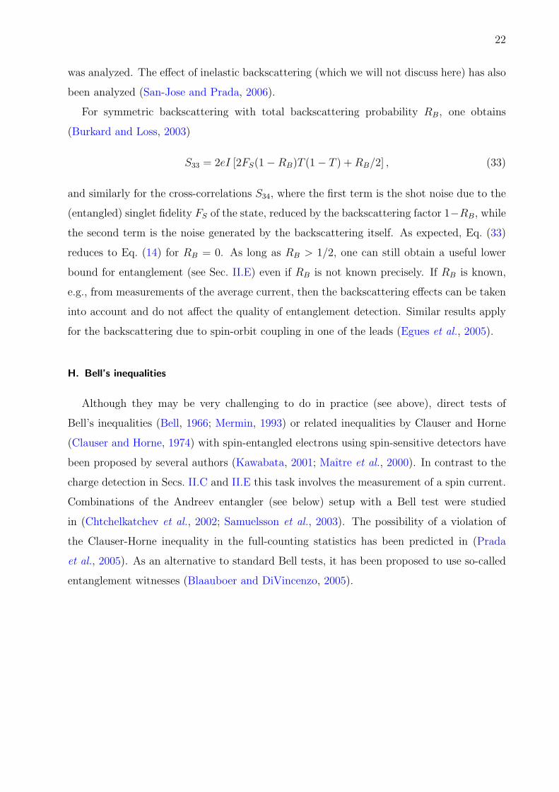
For symmetric backscattering with total backscattering probability RB, one obtains

(Burkard and Loss, 2003)

S33 = 2eI [2FS(1−RB)T (1− T ) +RB/2] , (33)

and similarly for the cross-correlations S34, where the first term is the shot noise due to the

(entangled) singlet fidelity FS of the state, reduced by the backscattering factor 1−RB, while

the second term is the noise generated by the backscattering itself. As expected, Eq. (33)

reduces to Eq. (14) for RB = 0. As long as RB > 1/2, one can still obtain a useful lower

bound for entanglement (see Sec. II.E) even if RB is not known precisely. If RB is known,

e.g., from measurements of the average current, then the backscattering effects can be taken

into account and do not affect the quality of entanglement detection. Similar results apply

for the backscattering due to spin-orbit coupling in one of the leads (Egues et al., 2005).

H. Bell’s inequalities

Although they may be very challenging to do in practice (see above), direct tests of

Bell’s inequalities (Bell, 1966; Mermin, 1993) or related inequalities by Clauser and Horne

(Clauser and Horne, 1974) with spin-entangled electrons using spin-sensitive detectors have

been proposed by several authors (Kawabata, 2001; Maıtre et al., 2000). In contrast to the

charge detection in Secs. II.C and II.E this task involves the measurement of a spin current.

Combinations of the Andreev entangler (see below) setup with a Bell test were studied

in (Chtchelkatchev et al., 2002; Samuelsson et al., 2003). The possibility of a violation of

the Clauser-Horne inequality in the full-counting statistics has been predicted in (Prada

et al., 2005). As an alternative to standard Bell tests, it has been proposed to use so-called

entanglement witnesses (Blaauboer and DiVincenzo, 2005).

23

FIG. 7 Schematic of the Andreev entangler as proposed in (Recher et al., 2001). Andreev tunneling

takes place as follows: A Cooper pair in the superconductor (SC) is separated into two spin-

entangled electrons which tunnel with amplitude TSD from two points r1, r2 of the SC onto the

two quantum dots 1 and 2. The dots are coupled to normal leads 1 and 2 with tunneling amplitude

TDL. The entangler will be most efficient for asymmetric barriers, |TSD|/|TDL| � 1.

III. PRODUCTION OF SPIN ENTANGLEMENT

A. Superconductor-normal junctions

The condensate in a conventional superconductor (SC) with s-wave pairing symmetry

consists of a large number of Cooper pairs that are in the spin singlet state Eq. (1). A

device that harnesses this large reservoir of entangled singlets has been proposed in (Recher

et al., 2001): It consists of a SC contact (at the chemical potential µS) from which quantum

tunneling of single electrons to two quantum dots D1 and D2 is possible with a quantum

amplitude TSD. The quantum dots, in turn, are coupled with tunneling amplitude TDL to

the normal leads L1 and L2 (both at the chemical potential µ1 = µ2), see Fig. 7.

The desired physical process for entanglement generation is Andreev tunneling where

two electrons (one with spin up and another one with spin down) tunnel coherently through

a normal barrier (Hekking et al., 1993). At the same time, single-particle tunneling is

suppressed by the presence of the intermediate quantum dots, forcing the two electrons

from a Cooper pair to tunnel coherently into separate leads rather than both into the same

lead. The double occupation of a quantum dot is suppressed by the Coulomb blockade

24

mechanism (Kouwenhoven et al., 1997). The transport of entangled electrons from the SC

the the quantum dots and from there to the normal leads can be controlled with an applied

bias voltage ∆µ = µS − µl > 0 (l = 1, 2).

The parameter regime for the generation of spin-entangled electrons is discussed in

(Recher et al., 2001): The barriers of the quantum dots need to be asymmetric, |TSD| �

|TDL|, the temperature must be sufficiently small, ∆µ > kBT , and ∆, U, δε > ∆µ > γl, kBT ,

and γl > γS, where ∆ is the SC energy gap, δε is the single-level spacing of the dots, and

γl = 2πνl|TSD|2 are the tunneling rates from lead l to the quantum dot (and vice versa).

The quality of the device is characterized by the ratio between the current I1 of pairwise

entangled electrons tunneling into different leads and the leakage current I2 of electron pairs

that end up in the same lead (Recher et al., 2001),

I1I2

=2E2

γ2

[sin(kF δr)

kF δr

]2

e−2δr/πξ, (34)

1

E=

1

π∆+

1

U. (35)

Here, kF denotes the Fermi wavevector, γ = γ1 + γ2, and ξ the SC coherence length.

The desired current I1 decreases exponentially with increasing distance δr = |r1 − r2|

between the tunneling points on the SC, the scale given by the superconducting coherence

length ξ. With ξ typically being on the order of µm, this does not pose severe restrictions

for a conventional s-wave SC. In the important case 0 ≤ δr ∼ ξ the suppression is only

polynomial ∝ 1/(kF δr)2, with kF being the Fermi wavevector in the SC. One also observes

that the effect of the quantum dots consists in the suppression factor (γ/E)2 for tunneling

into the same lead. One therefore has to impose the additional condition kF δr < E/γ, which

can be satisfied for small dots with E/γ ≈ 100 and k−1F ≈ 1 A.

Electron entangler devices with a SC reservoir attached to normal leads have also been

investigated in (Lesovik et al., 2001; Prada and Sols, 2004; Sauret et al., 2004). The presence

of voltage noise on the two quantum dots can lead to a reduction of the ratio Eq. (34), as

analyzed in (Dupont and Hur, 2006).

Shot noise and conductance measurements have been achieved in a quasi-ballistic SC-

normal beam-splitter junction (Choi et al., 2005). Moreover, transport properties of struc-

tures with a SC lead attached to normal leads have been studied experimentally (Russo

et al., 2005).

25

FIG. 8 The entangler as proposed

in (Recher and Loss, 2002a,b),

with a superconductor (SC) tunnel-

coupled to two one-dimensional

wires at positions r1 and r2 on the

SC with tunneling amplitude t0.

B. Superconductor-Luttinger liquid junctions

The production of electron spin entanglement requires interaction between the electrons;

in the case discussed in the previous Sec. III.A, the repulsive Coulomb interaction in the

quantum dots attached to the SC reservoir is used to separate the two entangled electrons.

Alternatively, a resistive lead where the dynamical Coulomb blockade effect helps to separate

the electron pair has been proposed (Recher and Loss, 2003).

A strongly interacting electron system in one spatial dimension can be described as a

Luttinger liquid (Tsvelik, 2003). A Luttinger liquid opens another possibility to separate

entangled electrons from a SC (Bena et al., 2002; Recher and Loss, 2002a,b). Physical sys-

tems with Luttinger liquid behavior are e.g. metallic carbon nanotubes (Egger and Gogolin,

1997; Kane et al., 1997). The setup studied theoretically in (Recher and Loss, 2002a,b) is

composed of two separate one-dimensional conductors (e.g., carbon nanotubes), each form-

ing a Luttinger liquid, which are tunnel-coupled (at a point far from their ends) to a SC,

see Fig. 8. The two wires are assumed to be sufficiently separated, such that interactions

between carriers in different wires can be neglected.

The fundamental excitations of a Luttinger liquid (if backscattering is absent) are long-

wavelength charge and spin density waves propagating with velocities uρ = vF/Kρ (charge)

and uσ = vF (spin) (Schulz, 1990), with vF the Fermi velocity and Kρ < 1 for an interacting

system. The tunneling of electrons from the SC to the one-dimensional (Luttinger liquid)

wires is modeled by the Hamiltonian

HT = t0∑ns

ψ†nsΨs(rn) + H.c., (36)

26

where Ψs(rn) is the annihilation (field) operator for an electron with spin s at the location rn

in the SC nearest to the one-dimensional wire n = 1, 2, and ψ†ns is the operator that creates

an electron at the coordinate xn in the wire n. Applying a bias µ = µS − µl between the

SC (with chemical potential µS) and the leads (µl) induces the flow of a stationary current

of pairwise spin-entangled from the SC to the one-dimensional wires.

Similar to the case of the Andreev entangler with attached quantum dots, discussed in

Sec. III.A above, the performance of this device can be quantified by the ratio between the

two competing currents, I1 for electrons tunneling into separate leads, thus contributing to

entanglement between the remote parts of the system, and I2 for electrons tunneling into

the same lead, thus not contributing to entanglement. From a T-matrix calculation (Recher

and Loss, 2002a,b), one obtains in leading order in µ/∆, where ∆ denotes the SC excitation

gap, and at zero temperature,

I1 =I01

Γ(2γρ + 2)

vF

uρ

[2Λµ

uρ

]2γρ

, (37)

I01 = 4πeγ2µ

sin2(kF δr)

(kF δr)2e−2δr/πξ, (38)

I2 = I1(δr → 0)∑b=±1

Ab

(2µ

∆

)2γρb

, (39)

where Γ is the Gamma function, Λ a short distance cut-off on the order of the lattice spacing

in the Luttinger liquid, γ = 2πνSνl|t0|2 the probability per spin to tunnel from the SC to

the one-dimensional leads, νS and νl the energy DOS per spin for the SC and the one-

dimensional leads at the chemical potentials µS and µl, respectively, and δr the separation

between the tunneling points on the SC. The constant Ab is of order one and does not

depend on the interaction strength. Furthermore, we have used the definitions γρ+ = γρ and

γρ− = γρ+ + (1−Kρ)/2 > γρ+. Note that in Eq. (39), the current I1 needs to be evaluated

at δr = 0. In the non-interacting limit, I2 = I1 = I01 is obtained by putting γρ = γρb = 0,

and uρ = vF .

In order to obtain a finite measurable current, the coherence length ξ of the Cooper

pairs should exceed δr (as in Sec. III.A for the Andreev entangler). It has been argued

that the suppression of the current by 1/(kF δr)2 can be considerably reduced by using low-

dimensional SCs (Recher and Loss, 2002a,b). The undesired injection of two electrons into

the same lead (current I2) is suppressed compared to I1 by a factor of (2µ/∆)2γρ+ , where

γρ+ = γρ, if the two electrons are injected into the same direction (left or right movers), or

27

by (2µ/∆)2γρ− if they propagate in different directions. The first scenario (same direction) is

the more likely one since γρ− > γρ+. The suppression of I2 by 1/∆ is due to the two-particle

correlations in the Luttinger liquid when the electrons tunnel into the same lead, similar to

the Coulomb blockade effect for tunneling into quantum dots in the previous Sec. III.A. The

delay time between the two electrons from the same Cooper pair is controlled by the inverse

SC gap ∆−1, i.e., if ∆ becomes larger, the electrons arrive within a shorter time interval,

thus increasing the correlations and further suppressing the unwanted I2. Increasing the

bias µ has the opposite effect, since it opens up more available states into which the electron

can tunnel, and therefore the effect of the SC gap ∆ is mitigated.

Noise correlations in the current carried by the entangled electrons emitted by a carbon

nanotube–SC entangler are studied in (Bouchiat et al., 2003).

C. Quantum dots coupled to normal leads

The Coulomb interaction between electrons in a quantum dot has also been suggested

as the main mechanism in electron spin entanglers with normal (as opposed to SC) leads.

An entangler comprising a single quantum dot attached to special leads with a very narrow

bandwidth (Oliver et al., 2002) or with three coupled quantum dots (Saraga and Loss, 2003)

coupled to ordinary leads have been analyzed. The idea behind both proposals is to extract

the singlet ground state of a single quantum dot occupied by two electrons by moving

the two electrons into two separate leads. In both proposals, the separation is enhanced

due to two-particle energy conservation. Different ideas using double-dot turnstile devices

with time-dependent barriers were followed in (Blaauboer and DiVincenzo, 2005; Hu and

Das Sarma, 2004).

D. Coulomb scattering in a 2D electron system

Motivated by scanning probe imaging and control of electron flow in a two-dimensional

electron system in a semiconductor heterostructure (Topinka et al., 2000, 2001), it has

been proposed to use this technique to generate electron spin entanglement by controlling

Coulomb scattering in a interacting 2D electron system (Saraga et al., 2004, 2005). For

a scattering angle of π/2, constructive two-particle interference is expected to lead to an

28

enhancement of the spin-singlet scattering probability, and at the same time, a reduction of

the triplet scattering. These scattering amplitudes (and probabilities) have been obtained

using the Bethe-Salpeter equation for small rs, which in turn allowed for an estimate of the

achievable current of spin-entangled electrons (Saraga et al., 2004, 2005).

E. Other spin entangler proposals

In (Costa and Bose, 2001), the use of a magnetic impurity in a special beam-splitter

geometry was proposed for the purpose of generating spin entanglement between ballistic

electrons in a two-dimensional electron system. The process where two magnetic impurities

become entangled via electron scattering has been described more recently (Costa et al.,

2006).

The generation of entanglement using two-particle interference in combination with

which-way detection (charge detection) has been discussed in (Bose and Home, 2002).

The use of a sole carbon nanotube to create spin entanglement between a localized and

an itinerant electron has been suggested in (Gunlycke et al., 2006).

Entanglement between electrons subject to the spin-orbit interaction in a quantum dot,

in the absence of interaction, has been discussed in (Frustaglia et al., 2006).

IV. TRANSPORT OF ENTANGLED ELECTRONS

An electron spin qubit does not travel “on its own”—it is always attached to the electron’s

charge. This is an enormous advantage for many reasons, one being that spin information

can be converted into charge information which then allows sensitive read-out (Loss and

DiVincenzo, 1998). Another advantage, of interest in the present context, is that the charge

responds to externally applied fields and therefore electron spin qubits can in principle be

transported in an electric conductor.

This has prompted the question whether a pair of entangled electron spins could be pro-

duced in one location on a semiconductor structure and subsequently distributed over some

distance on-chip, to be consumed later for some quantum information task (see Sec. I.A).

Such transport has certainly reached quite an advanced level for photon qubits, reaching

distances of kilometers (Gisin et al., 2002). Even for modest distances, perhaps microme-

29

ters, within, e.g., a semiconductor structure, this is not straight-forward for electrons. An

electron that is injected into a metallic wire becomes immersed into a sea of other electrons

that (i) are indistinguishable from the injected electron, and (ii) interact with all other elec-

trons, including the injected one. Here, we report on the theoretical discussion regarding the

stability of spin entanglement an interacting many-electron system (Burkard et al., 2000;

DiVincenzo and Loss, 1999). To anticipate the main results, it turns out that the indis-

tinguishability of particles is harmless for spin entanglement, whereas Coulomb interactions

do affect entanglement, but only to some extent because the electron-electron interactions

are typically screened (Mahan, 1993). As discussed in more detail below, an electron being

added to the a metallic wire in the orbital state q will be “dressed” by the interactions on

a very short time scale (inverse plasma frequency). The resulting state has a quasiparticle

weight in state q which is renormalized by a factor zf with 0 ≤ zq ≤ 1. The weight zq

quantifies how likely it is to find an electron in the original state q, while 1− zq is the part

that is distributed among all the other states.

We can describe the time evolution of the entangled triplet or singlet states in the inter-

acting many-electron system by introducing the 2-particle Green’s function

Gt/s(12,34; t) =⟨ψ

t/s12 , t|ψ

t/s34

⟩, (40)

where we use the second-quantized notation introduced in Eq. (8) above. The singlet/triplet

Green’s function defined in Eq. (40) above can be expressed in terms of the standard two-

particle Green’s function (Mahan, 1993) G(12, 34; t) by

Gt/s(12,34; t) = −1

2

∑σ

[G(12, 34; t)±G(12, 34; t)] , (41)

where n = (n, σ) and n = (n,−σ). The + sign stands for the triplet (t), the − sign for the

singlet (s), Green’s function. If at time t = 0, a spin triplet (singlet) state is prepared, then

we can define the fidelity of transmission as the probability for finding a triplet (singlet)

after time t,

P (t) = |Gt/s(12,12; t)|2. (42)

To calculate the fidelity Eq. (42), we can therefore use Eq. (41) to reduce the problem to

that of calculating the (standard) two-particle Green’s function

G(12, 34; t) = −⟨Ta1(t)a2(t)a

†3a

†4

⟩(43)

30

for a time- and spin-independent Hamiltonian, H = H0 +∑

i<j Vij, where H0 describes the

free motion of N electrons, and Vij is the bare Coulomb interaction between electrons i and

j, 〈...〉 denotes the zero-temperature expectation value, and T is the time-ordering operator.

In the case where the leads are sufficiently separated, the vertex part in G(12, 34; t) vanishes,

and thus the two-particle Green’s function can be expressed in terms of interacting single-

particle Green’s functions G(n, t) via

G(12, 34; t) = G(13, t)G(24, t)−G(14, t)G(23, t), (44)

where (l = 1, 2)

G(n, t) = −i〈ψ0|Tan(t)a†n|ψ0〉 ≡ Gl(q, t). (45)

For the singlet/triplet Green’s functions, this leads, with Eq. (41), to

Gt/s(12,34; t) = −G(1, t)G(2, t)[δ13δ24 ∓ δ14δ23]. (46)

At t = 0 (or as long as interactions are absent) one finds G(n, t) = −i and Gt/s = δ13δ24 ∓

δ14δ23, the fidelity remains P = 1. Under the influence of interactions and for times 0 ≤

t . 1/Γq shorter than the quasiparticle lifetime 1/Γq, one can use the standard result for

particle energies εq = q2/2m near the Fermi energy εF (Mahan, 1993),

G1,2(q, t) ≈ −izqθ(εq − εF )e−iεqt−Γqt. (47)

In a two-dimensional electron system (2DES), e.g. in a GaAs heterostructure, one finds

Γq ∝ (εq−εF )2 log(εq−εF ) (Giuliani and Quinn, 1982) using the random phase approximation

(RPA) to take into account the screening of the Coulomb interaction (Mahan, 1993). It

remains to evaluate the quasiparticle weight at the Fermi surface,

zF =

(1− ∂

∂ωRe Σret(kF , ω)

)−1 ∣∣∣ω=0

, (48)

where Σret(q, ω) is the retarded irreducible self-energy. The fidelity can then be expressed

through zF as

P = z4F . (49)

This can be seen by evaluating the two-particle Green’s function for momenta q near the

Fermi surface, assuming that the two leads that carry the two entangled particles are iden-

tical (G1 = G2). One finds |Gt/s(12,34; t)|2 = z4F | δ13δ24 ∓ δ14δ23|2, for sufficiently short

times, 0 < t . 1/Γq.

31

Finally, in order to evaluate the quasiparticle weight factor, Eq. (50), we need the the

irreducible self-energy Σret. For a two-dimensional electron system (2DES), this quantity

has been evaluated explicitly in leading order of the interaction parameter rs = 1/kFaB,

where aB = ε0~2/me2 is the Bohr radius, in (Burkard et al., 2000; DiVincenzo and Loss,

1999), with the result

zF =1

1 + rs (1/2 + 1/π). (50)

This result has been extended to include corrections due to the Rashba spin-orbit interaction

(Saraga and Loss, 2005) and finite temperatures (Galitski and Sarma, 2004). In a standard

GaAs 2DES, one can estimate aB = 10.3 nm and rs = 0.614, which yields a quasiparticle

weight of zF = 0.665. Numerical evaluation of the RPA self-energy, summing up all orders

of rs within this approximation, yield the more accurate result zF = 0.691. Substituting

zF back into Eq. (49), we obtain approximately P ≈ 0.2. For larger electron density, i.e.,

smaller rs, one can expect P to be closer to one. It also needs to be stressed that P is

a fidelity without postselection. Typically, it is sufficient to count only the fidelity of the

postselected singlet pairs, i.e., those that can successfully be retrieved from the Fermi sea.

This postselected fidelity is not affected by the (spin-independent) Coulomb interaction at

all, i.e., Ppostsel = 1, provided that spin-scattering effects are negligible. The degree to which

spin-scattering events are really negligible can be quantified from experiments that measure

the spin coherence length (Awschalom and Kikkawa, 1999; Kikkawa and Awschalom, 1998;

Kikkawa et al., 1997). In these experiments, it was found that the spin coherence length

can exceed 100µm in in GaAs 2DES’s.

References

Aspect, A., J. Dalibard, and G. Roger, 1982, Phys. Rev. Lett. 49, 1804.

Averin, D. V., and Y. V. Nazarov, 1992, in Single Charge Tunneling, edited by H. Grabert and

M. H. Devoret (Plenum Press, New York), volume 294 of NATO ASI Series B: Physics.

Awschalom, D. D., and J. M. Kikkawa, 1999, Phys. Today 52(6), 33.

Beenakker, C. W. J., 2006 (IOS Press, Amsterdam), volume 162 of Proc. Int. School Phys. E.

Fermi, cond-mat/9906071.

Bell, J. S., 1966, Rev. Mod. Phys. 38, 447.

Bena, C., S. Vishveshwara, L. Balents, and M. P. A. Fisher, 2002, Phys. Rev. Lett. 89, 037901.

32

Bennett, C. H., G. Brassard, C. Crepeau, R. Jozsa, A. Peres, and W. K. Wootters, 1993, Phys.

Rev. Lett. 70, 1895.

Bennett, C. H., G. Brassard, S. Popescu, B. Schumacher, J. A. Smolin, and W. K. Wootters, 1996a,

Phys. Rev. Lett. 76, 722.

Bennett, C. H., and D. P. DiVincenzo, 2000, Nature 404, 247.

Bennett, C. H., D. P. DiVincenzo, J. A. Smolin, and W. K. Wootters, 1996b, Phys. Rev. A 54,

3824.

Bennett, C. H., and S. J. Wiesner, 1992, Phys. Rev. Lett. 69, 2881.

Blaauboer, M., and D. P. DiVincenzo, 2005, Phys. Rev. Lett. 95(16), 160402.

Blanter, Y. M., and M. Buttiker, 2000, Phys. Rep. 336, 1.

Borlin, J., W. Belzig, and C. Bruder, 2002, Phys. Rev. Lett. 88, 197001.

Boschi, D., S. Branca, F. De Martini, L. Hardy, and S. Popescu, 1998, Phys. Rev. Lett. 80, 1121.

Bose, S., and D. Home, 2002, Physical Review Letters 88(5), 050401.

Bouchiat, V., N. Chtchelkatchev, D. Feinberg, G. B. Lesovik, T. Martin, and J. Torres, 2003,

Nanotechnology 14(1), 77.

Bouwmeester, D., J.-W. Pan, K. Mattle, M. Eibl, H. Weinfurter, and A. Zeilinger, 1997, Nature

390, 575.

Burkard, G., and D. Loss, 2003, Phys. Rev. Lett. 91, 087903.

Burkard, G., D. Loss, and D. P. DiVincenzo, 1999, Phys. Rev. B 59, 2070.

Burkard, G., D. Loss, and E. V. Sukhorukov, 2000, Phys. Rev. B 61, R16303, cond-mat/9906071.

Buttiker, M., 1990, Phys. Rev. Lett. 65, 2901.

Buttiker, M., 1992, Phys. Rev. B 46, 12485.

Cerletti, V., O. Gywat, and D. Loss, 2005, Phys. Rev. B 72(11), 115316.

Chen, Y., and R. A. Webb, 2006, Phys. Rev. Lett. 97, 066604.

Choi, B.-R., A. E. Hansen, T. Kontos, C. Hoffmann, S. Oberholzer, W. Belzig, C. Schonenberger,

T. Akazaki, and H. Takayanagi, 2005, Phys. Rev. B 72(2), 024501.

Choi, M.-S., C. Bruder, and D. Loss, 2000, Phys. Rev. B 62, 13569.

Chtchelkatchev, N. M., G. Blatter, G. B. Lesovik, and T. Martin, 2002, Phys. Rev. B 66, 161320.

Clauser, J. F., and M. A. Horne, 1974, Phys. Rev. D 10, 526.

Costa, A. T., and S. Bose, 2001, Phys. Rev. Lett. 87(27), 277901.

Costa, A. T., S. Bose, and Y. Omar, 2006, Phys. Rev. Lett. 96(23), 230501.

33

Devetak, I., A. W. Harrow, and A. Winter, 2004, Phys. Rev. Lett. 93(23), 230504.

Di Lorenzo, A., and Y. V. Nazarov, 2005, Phys. Rev. Lett. 94(21), 210601.

DiVincenzo, D. P., and D. Loss, 1999, J. Mag. Magn. Matl. 200, 202.

Dowling, M. R., A. C. Doherty, and H. M. Wiseman, 2006, Phys. Rev. A 73(5), 052323.

Dupont, E., and K. L. Hur, 2006, Phys. Rev. B 73, 045325.

Egger, R., and A. Gogolin, 1997, Phys. Rev. Lett. 79, 5082.

Egues, J. C., G. Burkard, and D. Loss, 2002, Phys. Rev. Lett. 89, 176401.

Egues, J. C., G. Burkard, D. S. Saraga, J. Schliemann, and D. Loss, 2005, Phys. Rev. B 72, 235326.

Egues, J. C., P. Recher, D. S. Saraga, V. N. Golovach, G. Burkard, E. V. Sukhorukov, and D. Loss,

2003, in Quantum Noise in Mesoscopic Physics (Kluwer, The Netherlands), volume 97 of NATO

Science Series, pp. 241–274, cond-mat/0210498.

Einstein, A., B. Podolsky, and N. Rosen, 1935, Phys. Rev. 47, 777.

Ekert, A. K., 1991, Phys. Rev. Lett. 67, 661.

Faoro, L., F. Taddei, and R. Fazio, 2004, Phys. Rev. B 69, 125326.

Frustaglia, D., S. Montangero, and R. Fazio, 2006, Phys. Rev. B 74(16), 165326.

Galitski, V. M., and S. D. Sarma, 2004, Phys. Rev. B 70(3), 035111.

Giovannetti, V., D. Frustaglia, F. Taddei, and R. Fazio, 2006, Phys. Rev. B 74(11), 115315.

Gisin, N., G. Ribordy, W. Tittel, and H. Zbinden, 2002, Rev. Mod. Phys. 74, 145.

Giuliani, G. F., and J. J. Quinn, 1982, Phys. Rev. B 26, 4421.

Gunlycke, D., J. H. Jefferson, T. Rejec, A. Ramsak, D. G. Pettifor, and G. A. D. Briggs, 2006,

Journal of Physics: Condensed Matter 18(21), S851.

Gywat, O., G. Burkard, and D. Loss, 2002, Phys. Rev. B 65, 205329.

Hanbury Brown, R., and R. Q. Twiss, 1956, Nature 177, 27.

Hanson, R., L. P. Kouwenhoven, J. R. Petta, S. Tarucha, and L. M. K. Vandersypen, 2006, Spins

in few-electron quantum dots, submitted to Rev. Mod. Phys. (cond-mat/0610433).

Hekking, F. W. J., L. I. Glazman, K. A. Matveev, and R. I. Shekhter, 1993, Phys. Rev. Lett. 70,

4138.

Henny, M., S. Oberholzer, C. Strunk, T. Heinzel, K. Ensslin, M. Holland, and C. Schonenberger,

1999, Science 284, 296.

Hohenester, U., 2002, Phys. Rev. B 66, 245323.

Hong, C. K., Z. Y. Ou, and L. Mandel, 1987, Phys. Rev. Lett. 59(18), 2044.

34

Hu, X., and S. Das Sarma, 2004, Phys. Rev. B 69, 115312.

Kane, C., L. Balents, and M. Fisher, 1997, Phys. Rev. Lett. 79, 5086.

Kawabata, S., 2001, J. Phys. Soc. Jpn. 70, 1210.

Khlus, V. A., 1987, Zh. Eksp. Teor. Fiz. 93, 2179.

Kikkawa, J. M., and D. D. Awschalom, 1998, Phys. Rev. Lett. 80, 4313.

Kikkawa, J. M., I. P. Smorchkova, N. Samarth, and D. D. Awschalom, 1997, Science 277, 1284.

Kouwenhoven, L. P., G. Schon, and L. L. Sohn (eds.), 1997, Mesoscopic Electron Transport, volume

345 of NATO ASI Series E (Kluwer Academic Publishers, Dordrecht).

Landauer, R., 1989, Physica D 38, 226.

Lesovik, G., T. Martin, and G. Blatter, 2001, Eur. Phys. J. B 24, 287.

Lesovik, G. B., 1989, Pis’ma Zh. Eksp. Teor. Fiz. 49, 513.

Lim, Y. L., and A. Beige, 2005, New J. Phys. 7, 155.

Liu, R. C., B. Odom, Y. Yamamoto, and S. Tarucha, 1998, Nature 391, 263.

Loss, D., and D. P. DiVincenzo, 1998, Phys. Rev. A 57(1), 120.

Loss, D., and E. V. Sukhorukov, 2000, Phys. Rev. Lett. 84, 1035.

Loudon, R., 1998, Phys. Rev. A 58, 4904.

Mahan, G. D., 1993, Many Particle Physics (Plenum, New York), 2nd edition.

Maıtre, X., W. D. Oliver, and Y. Yamamoto, 2000, Physica E 6, 301.

Martin, T., and R. Landauer, 1992, Phys. Rev. B 45, 1742.

Mattle, K., H. Weinfurter, P. G. Kwiat, and A. Zeilinger, 1996, Phys. Rev. Lett. 76, 4656.

Mermin, N. D., 1993, Rev. Mod. Phys. 65, 803.

Oberholzer, S., E. Bieri, C. Schonenberger, M. Giovannini, and J. Faist, 2006, Physical Review

Letters 96(4), 046804.

Oliver, W. D., J. Kim, R. C. Liu, and Y. Yamamoto, 1999, Science 284, 299.

Oliver, W. D., F. Yamaguchi, and Y. Yamamoto, 2002, Phys. Rev. Lett. 88, 037901.

Prada, E., and F. Sols, 2004, Eur. Phys. J. B 40, 379.

Prada, E., F. Taddei, and R. Fazio, 2005, Phys. Rev. B 72, 125333.

Prinz, G. A., 1998, Science 282, 1660.

Recher, P., and D. Loss, 2002a, Journal of Superconductivity and Novel Magnetism 15, 49, cond-

mat/0202102.

Recher, P., and D. Loss, 2002b, Phys. Rev. B 65, 165327.

35

Recher, P., and D. Loss, 2003, Phys. Rev. Lett. 91, 267003.

Recher, P., E. V. Sukhorukov, and D. Loss, 2001, Phys. Rev. B 63, 165314.

Russo, S., M. Kroug, T. M. Klapwijk, and A. F. Morpurgo, 2005, Phys. Rev. Lett. 95(2), 027002.

Samuelsson, P., E. V. Sukhorukov, and M. Buttiker, 2003, Phys. Rev. Lett. 91, 157002.

Samuelsson, P., E. V. Sukhorukov, and M. Buttiker, 2004, Phys. Rev. B 70, 115330.

San-Jose, P., and E. Prada, 2006, Phys. Rev. B 74(4), 045305.

Saraga, D. S., B. L. Altshuler, D. Loss, and R. M. Westervelt, 2004, Phys. Rev. Lett. 92, 246803.

Saraga, D. S., B. L. Altshuler, D. Loss, and R. M. Westervelt, 2005, Phys. Rev. B 71, 045338.

Saraga, D. S., and D. Loss, 2003, Phys. Rev. Lett. 90, 166803.

Saraga, D. S., and D. Loss, 2005, Phys. Rev. B 72(19), 195319.

Sauret, O., D. Feinberg, and T. Martin, 2004, Phys. Rev. B 70(24), 245313.

Schliemann, J., J. I. Cirac, M. Kus, M. Lewenstein, and D. Loss, 2001a, Phys. Rev. A 64, 022303.

Schliemann, J., D. Loss, and A. H. MacDonald, 2001b, Phys. Rev. B 63, 085311.

Schrodinger, E., 1935, Die Naturwissenschaften 23, 807.

Schulz, H. J., 1990, Phys. Rev. Lett. 64, 2831.

Sukhorukov, E. V., G. Burkard, and D. Loss, 2001, Phys. Rev. B 63, 125315.

Taddei, F., L. Faoro, E. Prada, and R. Fazio, 2005, New J. Phys. 7, 183.

Taddei, F., and R. Fazio, 2002, Phys. Rev. B 65, 075317.

Taylor, J. M., W. Dur, P. Zoller, A. Yacoby, C. M. Marcus, and M. D. Lukin, 2005, Phys. Rev.

Lett. 94, 236803.

Topinka, M. A., B. J. LeRoy, S. E. J. Shaw, E. J. Heller, R. M. Westervelt, K. D. Maranowski,

and A. C. Gossard, 2000, Science 289, 2323.

Topinka, M. A., B. J. Leroy, R. M. Westervelt, S. E. J. Shaw, R. Fleischmann, E. J. Heller, K. D.

Maranowski, and A. C. Gossard, 2001, Nature 410, 183.

Torres, J., and T. Martin, 1999, Eur. Phys. J. B 12, 319.

Tsvelik, A. M., 2003, Quantum Field Theory in Condensed Matter Physics (Cambridge University

Press), 2nd edition.

Werner, R. F., 1989, Phys. Rev. A 40, 4277.

Wiseman, H. M., and J. A. Vaccaro, 2003, Phys. Rev. Lett. 91(9), 097902.

Wootters, W. K., 1998, Phys. Rev. Lett. 80, 2245.