Spin 0 and spin 1/2 quantum relativisticparticles in a constant gravitational field

M. Khorrami,a,c,* M. Alimohammadi,b and A. Shariatia,c

a Institute for Advanced Studies in Basic Sciences, P.O. Box 159, Zanjan 45195, Iranb Department of Physics, University of Tehran, North Karegar Ave., Tehran, Iran

c Institute of Applied Physics, P.O. Box 5878, Tehran 15875, Iran

Received 3 November 2002

Abstract

The Klein–Gordon and Dirac equations in a semi-infinite lab (x > 0), in the backgroundmetric ds2 ¼ u2ðxÞð�dt2 þ dx2Þ þ dy2 þ dz2, are investigated. The resulting equations are stud-ied for the special case uðxÞ ¼ 1þ gx. It is shown that in the case of zero transverse-momen-tum, the square of the energy eigenvalues of the spin-1/2 particles are less than the squares of

the corresponding eigenvalues of spin-0 particles with same masses, by an amount of mg�hc.Finally, for non-zero transverse-momentum, the energy eigenvalues corresponding to large

quantum numbers are obtained and the results for spin-0 and spin-1/2 particles are compared

to each other.

� 2003 Elsevier Science (USA). All rights reserved.

1. Introduction

The behaviour of bosons and fermions in a gravitational field has been of interest

for many years, from the simplest case of a non-relativistic quantum particle in the

presence of constant gravity, [1] for example, to more complicated cases of the rela-

tivistic spin-1/2 particles in a curved space-time with torsion, [2,3] for example. Sev-

eral experiments have been performed to test theoretical predictions, among which

are the experiments of Colella et al. [4], which detected gravitational effects by neu-

tron interferometry, and the recent experiment of Nesvizhevsky et al. [5], in whichthe quantum energy levels of neutrons in the Earth�s gravity were detected.

Annals of Physics 304 (2003) 91–102

www.elsevier.com/locate/aop

*Corresponding author.

E-mail addresses: mamwad@mailaps.org (M. Khorrami), alimohmd@ut.ac.ir (M. Alimohammadi).

0003-4916/03/$ - see front matter � 2003 Elsevier Science (USA). All rights reserved.

doi:10.1016/S0003-4916(03)00016-2

Chandrasekhar considered the Dirac equation in a Kerr-geometry background

and separated the Dirac equation into radial and angular parts [6,7]. In [8], the an-

gular part was solved and in [9] some semi-analytical results for the radial part were

obtained. Similar calculations were performed for the Kerr–Newman geometry and

around dyon black holes in [10,11], respectively.In this article, we investigate relativistic spin-0 and spin-1/2 particles in a back-

ground metric ds2 ¼ u2ðxÞð�dt2 þ dx2Þ þ dy2 þ dz2, where the particles exist in asemi-infinite laboratory (x > 0). The wall x ¼ 0, which prevents particles from pene-trating to the region x < 0, corresponds to a boundary condition. For spin-0 parti-cles, this is simply the vanishing of wave function on the wall. For the spin-1/2

particles, it is less trivial and will be discussed in the article. We consider the Ham-

iltonian-eigenvalue problems corresponding to a general function uðxÞ, and obtainthe differential equations and boundary conditions corresponding to the spin-0and spin-1/2 particles. The special case, uðxÞ ¼ 1þ gx, is investigated in more detail.An exact relation between the square of the energy eigenvalues of spin-0 and spin-1/2

particles, with same masses and no transverse momenta, is obtained, namely

E2D ¼ E2KG � mg�hc. Finally, the energy eigenvalues for large energies are obtained.

2. Review of the non-relativistic problem

The potential energy of a non-relativistic particle in a constant gravitational field

is VgravðxÞ ¼ mgx, where g is the acceleration of gravity, the direction of which isalong the x-axis, towards the negative values of x.The Schr€oodinger equation is written as HwSch ¼ i�hotwSch, where H ¼ P2=ð2mÞþ

Vgrav, subject to the boundary conditions that wSch does not diverge at x ! �1.Writing wSch ¼ exp½ð�iEt þ ip2y þ ip3zÞ=�hF ðxÞ, it is easily seen that F ðxÞ must sat-

isfy F 00ðxÞ ¼ ðL�3xþ L�2kSchÞF ðxÞ, where a prime means differentiation with respectto the argument, L�2kSch :¼ ðp22 þ p23 � 2mEÞ=ð�h2Þ and L :¼ ð2m2g=�h2Þ�1=3. This equa-tion has two linearly independent solutions: the Airy functions AiðL�1xþ kSchÞ andBiðL�1xþ kSchÞ (see, for example, [12, p. 569]). Bi violates the boundary conditionat þ1. So the solutions are AiðL�1xþ kSchÞ. These functions do not tend to zeroat x ! �1, and it is expected, since the potential mgx is not bounded from below.

But we note that a lab usually has walls. Consider a semi-infinite lab, for which

Vwalls ¼þ1; x < 0;0; xP 0:

�ð1Þ

In such a lab, the boundary condition at �1 is replaced with limx!0þ wSch ¼ 0: Sothe solutions are AiðL�1xþ kSchÞ, where kSch must be one of the zeros of Ai.The first four zeros of Ai are approximately k1 ¼ �2:3381, k2 ¼ �4:0879, k3 ¼

�5:5206, and k4 ¼ �6:7867. If the transverse momenta of the particle vanish, the en-ergy levels are these numbers multiplied by ��h2=3ð2mÞ1=3ðg=2Þ2=3, the value of whichfor a neutron, in a lab on the Earth, where g ffi 9:8ms�2, is 0:59peV. Therefore, thefirst four energy levels of a neutron are E1 ¼ 1:4peV, E2 ¼ 2:5peV, E3 ¼ 3:3peV, andE4 ¼ 4:0peV. This result has been recently verified experimentally [5].

92 M. Khorrami et al. / Annals of Physics 304 (2003) 91–102

3. A relativistic quantum particle

According to general relativity, gravity is represented by a pseudo-Riemannian

metric ds2 ¼ glm dxl dxm. We use the signature ð� þ þþÞ for the metric. The formof the metric depends on both the gravitational field and the coordinate system usedto describe the field.

In a space-time with metric glm, the Klein–Gordon equation, the equation for a

spinless massive particle, is

1ffiffiffiffiffiffiffi�gp

o

oxl

ffiffiffiffiffiffiffi�gp

glm o

oxm

�� m2

�wKG ¼ 0;

where g :¼ det ½glm. We have used a system of units in which the numerical

values of the velocity of light (c) and the Planck constant (divided by 2p) areboth unity.To write the Dirac equation in a curved space-time, or a flat space-time but in

a curvilinear coordinate system, one can employ the Equivalence Principle—see,

for example, [13, pp. 365–373], but note that our convention for the Dirac La-

grangian, and therefore the Dirac equation, is different from that of Weinberg:

we use ��m� in the following equation, instead of a �þm� in Weinberg�s. It readsas follows:

ca oað þ CaÞwD � mwD ¼ 0;where Cas are spin connections, obtained from the dual tetrad ea, through

dea þ Cab ^ eb ¼ 0;

Cab :¼ Ca

cb ec;

Ca :¼1

2Sbc Cc b

a ;

Sbc :¼ � 14

cb; cc½ :

We consider a gravitational field which is represented by the metric

ds2 ¼ u2ðxÞ�� dt2 þ dx2

�þ dy2 þ dz2: ð2Þ

One can write the above metric, also like

ds2 ¼ �U 2ðX Þ dt2 þ dX 2 þ dy2 þ dz2;

where ðdX Þ=ðdxÞ ¼ UðX Þ ¼ uðxÞ. In a small region of space (compared to the lengthin which the gravitational field changes significantly) one can use uðxÞ ¼ 1þ gx,UðX Þ ¼ 1þ gX , and X ¼ x. We will investigate the case of a general uðxÞ, but thenlimit ourselves to the special case uðxÞ ¼ 1þ gx.For the metric (2), the Klein–Gordon equation reads

1

u2

��� o2

ot2þ o2

ox2

�þ o2

oy2þ o2

oz2� m2

�wKG ¼ 0:

M. Khorrami et al. / Annals of Physics 304 (2003) 91–102 93

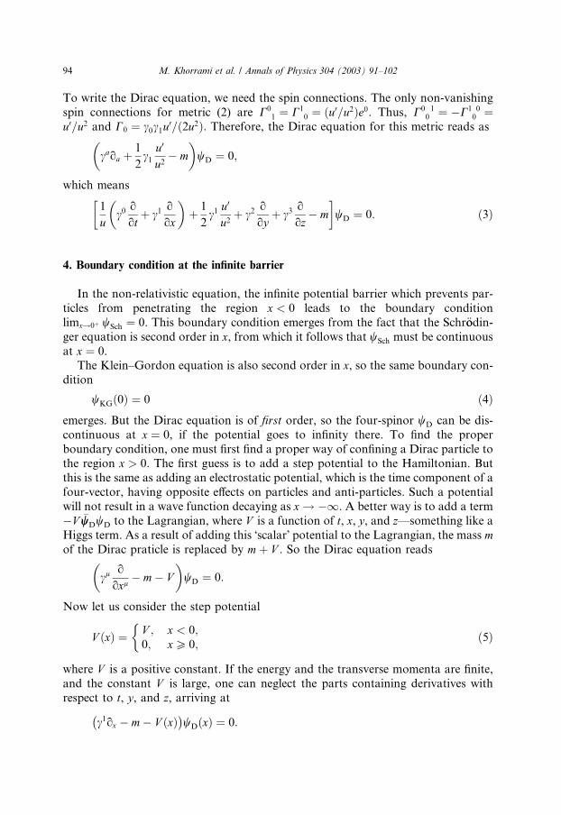
To write the Dirac equation, we need the spin connections. The only non-vanishing

spin connections for metric (2) are C01 ¼ C10 ¼ ðu0=u2Þe0. Thus, C0 10 ¼ �C1 00 ¼

u0=u2 and C0 ¼ c0c1u0=ð2u2Þ: Therefore, the Dirac equation for this metric reads as

caoa

�þ 12c1

u0

u2� m

�wD ¼ 0;

which means

1

uc0

o

ot

��þ c1

o

ox

�þ 12

c1u0

u2þ c2

o

oyþ c3

o

oz� m

�wD ¼ 0: ð3Þ

4. Boundary condition at the infinite barrier

In the non-relativistic equation, the infinite potential barrier which prevents par-

ticles from penetrating the region x < 0 leads to the boundary condition

limx!0þ wSch ¼ 0. This boundary condition emerges from the fact that the Schr€oodin-ger equation is second order in x, from which it follows that wSch must be continuousat x ¼ 0.The Klein–Gordon equation is also second order in x, so the same boundary con-

dition

wKGð0Þ ¼ 0 ð4Þemerges. But the Dirac equation is of first order, so the four-spinor wD can be dis-continuous at x ¼ 0, if the potential goes to infinity there. To find the properboundary condition, one must first find a proper way of confining a Dirac particle tothe region x > 0. The first guess is to add a step potential to the Hamiltonian. Butthis is the same as adding an electrostatic potential, which is the time component of a

four-vector, having opposite effects on particles and anti-particles. Such a potential

will not result in a wave function decaying as x ! �1. A better way is to add a term�V �wwDwD to the Lagrangian, where V is a function of t, x, y, and z—something like aHiggs term. As a result of adding this �scalar� potential to the Lagrangian, the mass mof the Dirac praticle is replaced by mþ V . So the Dirac equation reads

cl o

oxl

�� m� V

�wD ¼ 0:

Now let us consider the step potential

V ðxÞ ¼ V ; x < 0;0; xP 0;

�ð5Þ

where V is a positive constant. If the energy and the transverse momenta are finite,and the constant V is large, one can neglect the parts containing derivatives with

respect to t, y, and z, arriving at

c1ox�

� m� V ðxÞ�wDðxÞ ¼ 0:

94 M. Khorrami et al. / Annals of Physics 304 (2003) 91–102

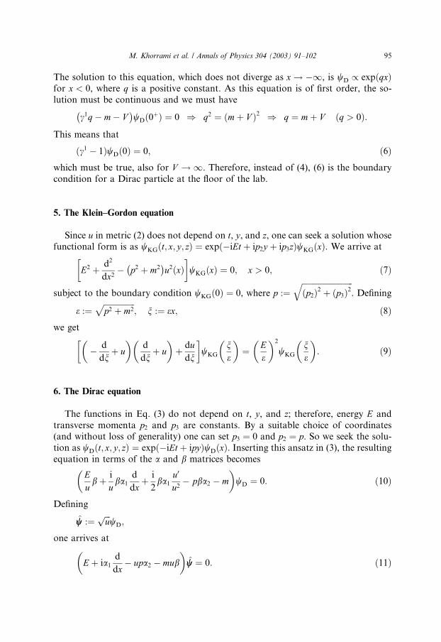
The solution to this equation, which does not diverge as x ! �1, is wD / expðqxÞfor x < 0, where q is a positive constant. As this equation is of first order, the so-lution must be continuous and we must have

c1q�

� m� V�wDð0þÞ ¼ 0 ) q2 ¼ ðmþ V Þ2 ) q ¼ mþ V ðq > 0Þ:

This means that

ðc1 � 1ÞwDð0Þ ¼ 0; ð6Þwhich must be true, also for V ! 1. Therefore, instead of (4), (6) is the boundarycondition for a Dirac particle at the floor of the lab.

5. The Klein–Gordon equation

Since u in metric (2) does not depend on t, y, and z, one can seek a solution whosefunctional form is as wKGðt; x; y; zÞ ¼ expð�iEt þ ip2y þ ip3zÞwKGðxÞ. We arrive at

E2�

þ d2

dx2� p2�

þ m2�u2ðxÞ

�wKGðxÞ ¼ 0; x > 0; ð7Þ

subject to the boundary condition wKGð0Þ ¼ 0, where p :¼ffiffiffiffiffiffiffiffiffiffiffiffiffiffiffiffiffiffiffiffiffiffiffiffiffiffiðp2Þ2 þ ðp3Þ2

q. Defining

e :¼ffiffiffiffiffiffiffiffiffiffiffiffiffiffiffiffip2 þ m2

p; n :¼ ex; ð8Þ

we get��� d

dnþ u

�d

dn

�þ u

�þ dudn

�wKG

ne

� �¼ E

e

� �2wKG

ne

� �: ð9Þ

6. The Dirac equation

The functions in Eq. (3) do not depend on t, y, and z; therefore, energy E andtransverse momenta p2 and p3 are constants. By a suitable choice of coordinates(and without loss of generality) one can set p3 ¼ 0 and p2 ¼ p. So we seek the solu-tion as wDðt; x; y; zÞ ¼ expð�iEt þ ipyÞwDðxÞ. Inserting this ansatz in (3), the resultingequation in terms of the a and b matrices becomes

Eu

b

�þ i

uba1

d

dxþ i

2ba1

u0

u2� pba2 � m

�wD ¼ 0: ð10Þ

Defining

ww :¼ffiffiffiu

pwD;

one arrives at

E�

þ ia1d

dx� upa2 � mub

�ww ¼ 0: ð11Þ

M. Khorrami et al. / Annals of Physics 304 (2003) 91–102 95

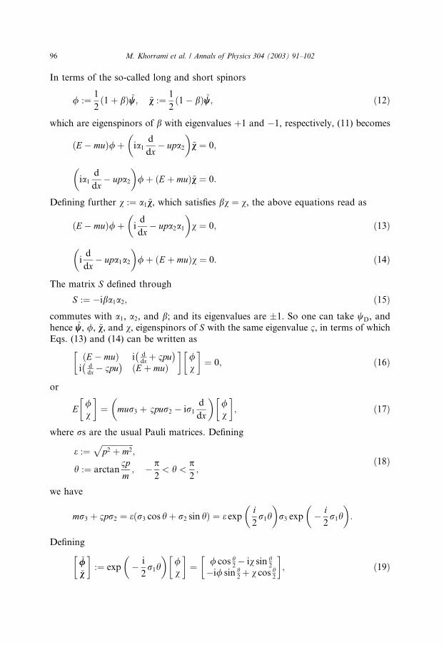
In terms of the so-called long and short spinors

/ :¼ 121ð þ bÞww; ~vv :¼ 1

21ð � bÞww; ð12Þ

which are eigenspinors of b with eigenvalues þ1 and �1, respectively, (11) becomes

ðE � muÞ/ þ ia1d

dx

�� upa2

�~vv ¼ 0;

ia1d

dx

�� upa2

�/ þ ðE þ muÞ~vv ¼ 0:

Defining further v :¼ a1~vv, which satisfies bv ¼ v, the above equations read as

ðE � muÞ/ þ id

dx

�� upa2a1

�v ¼ 0; ð13Þ

id

dx

�� upa1a2

�/ þ Eð þ muÞv ¼ 0: ð14Þ

The matrix S defined through

S :¼ �iba1a2; ð15Þcommutes with a1, a2, and b; and its eigenvalues are �1. So one can take wD, andhence ww, /, ~vv, and v, eigenspinors of S with the same eigenvalue 1, in terms of whichEqs. (13) and (14) can be written as

ðE � muÞ i ddx þ 1pu

� �i ddx � 1pu

� �ðE þ muÞ

� �/v

� �¼ 0; ð16Þ

or

E/v

� �¼ mur3

�þ 1pur2 � ir1

d

dx

�/v

� �; ð17Þ

where rs are the usual Pauli matrices. Defining

e :¼ffiffiffiffiffiffiffiffiffiffiffiffiffiffiffiffip2 þ m2

p;

h :¼ arctan 1pm; � p

2< h <

p2;

ð18Þ

we have

mr3 þ 1pr2 ¼ e r3 cos hð þ r2 sin hÞ ¼ e expi2

r1h

� �r3 exp

�� i2r1h

�:

Defining

�//�vv

� �:¼ exp

�� i

2r1h

�/v

� �¼ / cos h

2� iv sin h

2

�i/ sin h2þ v cos h

2

� �; ð19Þ

96 M. Khorrami et al. / Annals of Physics 304 (2003) 91–102

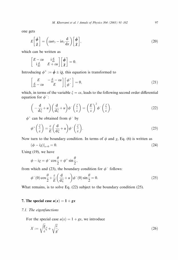
one gets

E�//�vv

� �¼ eur3

�� ir1

d

dx

��//�vv

� �; ð20Þ

which can be written as

E � eu i ddx

i ddx E þ eu

� ��//�vv

� �¼ 0:

Introducing /� :¼ �// � i�vv, this equation is transformed to

E � ddx � eu

ddx � eu E

� �/þ

/�

� �¼ 0; ð21Þ

which, in terms of the variable n ¼ ex, leads to the following second order differentialequation for /�:

�� d

dnþ u

�d

dn

�þ u

�/� n

e

� �¼ E

e

� �2/� n

e

� �: ð22Þ

/þ can be obtained from /� by

/þ ne

� �¼ e

Ed

dn

�þ u

�/� n

e

� �: ð23Þ

Now turn to the boundary condition. In terms of / and v, Eq. (6) is written as

ð/ � ivÞjx¼0 ¼ 0: ð24ÞUsing (19), we have

/ � iv ¼ /� cosh2þ /þ sin

h2;

from which and (23), the boundary condition for /� follows:

/�ð0Þ cos h2þ eE

d

dn

�þ u

�/�ð0Þ sin h

2¼ 0: ð25Þ

What remains, is to solve Eq. (22) subject to the boundary condition (25).

7. The special case uðxÞ ¼ 1þ gx

7.1. The eigenfunctions

For the special case uðxÞ ¼ 1þ gx, we introduce

X :¼ffiffiffige

rn þ

ffiffiffieg

r; ð26Þ

M. Khorrami et al. / Annals of Physics 304 (2003) 91–102 97

and the Klein–Gordon equation (9) becomes��� d

dXþ X

�d

dX

�þ X

�þ 1

�fKGðX Þ ¼ k2KGfKGðX Þ; X P

ffiffiffieg

r; ð27Þ

where

k2KG :¼ E2KGge

;

and

fKGðX Þ :¼ wKGðxÞ:The boundary condition reads (see Eq. (4))

fKG

ffiffiffieg

r� �¼ 0: ð28Þ

For the Dirac equation, in this special case, again in terms of the variable X , Eq. (22)becomes�

� d

dXþ X

�d

dX

�þ X

�fDðX Þ ¼ k2DfDðX Þ; X P

ffiffiffieg

r; ð29Þ

where

k2D :¼ E2Dge

;

and

fDðX Þ :¼ /�ðxÞ:The boundary condition (25) is now

fD

ffiffiffieg

r� �cos

h2þ 1

kD

d

dX

�þ X

�fD

ffiffiffieg

r� �sin

h2¼ 0: ð30Þ

Comparing (27) and (29), and defining k2 ¼ k2KG � 1 for the Klein–Gordon equationand k2 ¼ k2D for the Dirac equation, we see that both of them are of the same form�

� d

dXþ X

�d

dX

�þ X

�f ðX Þ ¼ k2f ðX Þ; ð31Þ

but subject to different boundary conditions (28) and (30).

Note that this final equation is the same as the Schr€oodinger equation for a one-dimensional simple harmonic oscillator. The difference is that for the simple har-

monic oscillator, �1 < X < þ1; while in our caseffiffiffiffiffiffiffie=g

p< X < þ1, and that

we have the boundary condition (28) or (30) for X !ffiffiffiffiffiffiffie=g

p þ.

To solve (31), we define hðX Þ as

f ðX Þ ¼ hðX Þ exp�� 12X 2

�ð32Þ

98 M. Khorrami et al. / Annals of Physics 304 (2003) 91–102

and obtain

2X�

� d

dX

�dhdX

¼ k2h: ð33Þ

Now we seek a power-series solution for hðX Þ:

hðX Þ ¼X10

anX n:

Putting this in (33), one obtains

a2k ¼4k C k � k2

4

�

ð2kÞ!C � k2

4

� a0; ð34Þ

a2kþ1 ¼4k C k þ 1

2� k2

4

�

ð2k þ 1Þ!C 12� k2

4

� a1; ð35Þ

and from that the following two solutions:

h0ðX Þ ¼a0

C � k2

4

� X1k¼0

ð2X Þ2kC k � k2

4

�ð2kÞ! ; ð36Þ

h1ðX Þ ¼a1

2C 12� k2

4

� X1k¼0

ð2X Þ2kþ1C k þ 12� k2

4

�ð2k þ 1Þ! : ð37Þ

We have to find a linear combination of these two functions, which remains finite as

X ! 1. To do so, we define the function

SaðX Þ :¼X1k¼0

ð2X Þ2kþaC k þ a2� k2

4

�ð2k þ aÞ! ;

It is seen that h0 and h1 are proportional to S0 and S1, respectively. Using a steepest-descent analysis to obtain the large-X behavior of Sa, it is seen that this behavior is in

fact independent of a. This comes from the fact that if one replaces the summationover k with an integration, and change the variable k þ a into k, then the dependenceof S on a comes solely from the lower bound of the integration region. But this

bound is unimportant, since the major part of the sum comes from large k�s. In fact,one can perform the steepest descent analysis and find

SaðX Þ �X!1

X�1�k22 exp X 2

�þ 1þ k2

4

�:

M. Khorrami et al. / Annals of Physics 304 (2003) 91–102 99

So, h0ðX Þ þ h1ðX Þ remains finite as X ! 1, provideda1

2C 12� k2

4

� ¼ � a0

C � k2

4

� ¼: b:

So the unique (up to normalization) normalizable function which solves (31) is

hðX Þ :¼ bX1n¼0

ð�2X Þn C n2� k2

4

�n!

: ð38Þ

7.2. Comparing the energy eigenvalues

To compare the energies of three different Hamiltonians, namely the Schr€oodingerequation, the Klein–Gordon Eq. (27), and the Dirac Eq. (29), we reintroduce the

physical constants previously chosen to be equal to 1. One obtains

ESch ¼p2

2m� 2�1=3 kSch

�hgmc3

� �2=3mc2;

EKG ¼ kKG�hgmc3

� �1=2mc2 1

�þ p2

m2c2

�1=4;

ED ¼ kD�hgmc3

� �1=2mc2 1

�þ p2

m2c2

�1=4:

To compare kD and kKG, we first note that if p ¼ 0, then h ¼ 0 (see Eq. (18)).Therefore, the two boundary conditions (28) and (30) become the same and eigen-

value k2 in (31) becomes the same for the Klein–Gordon and the Dirac case. But k2 isequal to k2KG � 1 and k2D. So,

k2D ¼ k2KG � 1 for p ¼ 0;or

E2D ¼ E2KG � mg�hc for p ¼ 0: ð39ÞThis is an exact result which determines the effect of spin on the gravitational in-teraction of relativistic particles. A fermion and a boson with same masses have

different quantum energies when fall vertically in a constant gravitational field.

For p 6¼ 0, the relation between the eigenvalues is more complicated, because al-though the differential equations are the same, the boundary conditions are different.

In this case, it is possible to find approximate relations for kKG and kD, for large val-ues of them, and compare them in this region.

A WKB analysis of the wave function hðX Þ, performed in Appendix A, shows that

hðX Þ �k!1

cos pk2

4

�� kX

�: ð40Þ

100 M. Khorrami et al. / Annals of Physics 304 (2003) 91–102

Inserting (32) in (30), the boundary condition on hðX Þ for Dirac particles reads

hðX Þ cos h2

�þ 1

kD

dhdX

sinh2

�X¼

ffiffiffiffiffie=g

p���� ¼ 0;

which, using (40), leads to

cospk2D4

�� kDX � h

2

�X¼

ffiffiffiffiffie=g

p���� ¼ 0;

or

pk2D4

� kD

ffiffiffieg

r� h2¼ n

�þ 12

�p: ð41Þ

For the Klien–Gordon equation, from (28) and (32), it is seen that hðffiffiffiffiffiffiffie=g

pÞ ¼ 0.

Using (40), and remembering k2 ¼ k2KG � 1, we find

pk2KG4

� p4� kKG

ffiffiffieg

r¼ n

�þ 12

�p; ð42Þ

in which O(1=kKG) terms have been ignored. Comparing (41) and (42), results in

k2D ¼ k2KG � 1þ 2hp;

or

E2D ¼ E2KG �ffiffiffiffiffiffiffiffiffiffiffiffiffiffiffiffiffiffiffiffip2 þ m2c2

p�hg 1

�� 2

parctan

1pcm

�: ð43Þ

Appendix A. The asymptotic behaviour of the function hðXÞ

To obtain the asymptotic behaviour of hðX Þ, (38), for k � 1 and finite X , we firstwrite (38) as

hðX Þ ¼ bX1k¼0

ð2X Þ2k C k � k2

4

�ð2kÞ! � b

X1k¼0

ð2X Þ2kþ1C k þ 12� k2

4

�ð2k þ 1Þ! : ðA:1Þ

Using CðpÞCð1� pÞ ¼ p=ðsin ppÞ, we have

C k�

� k2

4

�¼ p

sin pðk � k2

4Þ

h iC k2

4� k þ 1

�

¼ � ð�1Þkpsin p k2

4

�C k2

4� k þ 1

� : ðA:2Þ

M. Khorrami et al. / Annals of Physics 304 (2003) 91–102 101

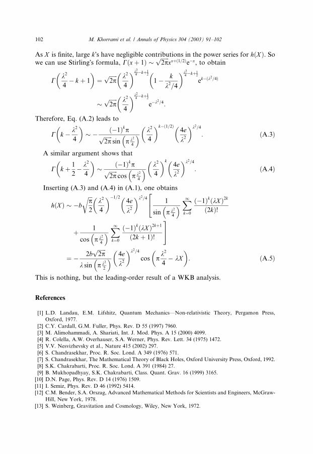
As X is finite, large k�s have negligible contributions in the power series for hðX Þ. Sowe can use Stirling�s formula, Cðxþ 1Þ �

ffiffiffiffiffiffi2p

pxxþð1=2Þe�x, to obtain

Ck2

4

�� k þ 1

�¼

ffiffiffiffiffiffi2p

p k2

4

� �k24�kþ1

2

1

�� k

k2=4

�k24�kþ1

2

ek�ðk2=4Þ

�ffiffiffiffiffiffi2p

p k2

4

� �k24�kþ1

2

e�k2=4:

Therefore, Eq. (A.2) leads to

C k�

� k2

4

�� � ð�1Þkpffiffiffiffiffiffi

2pp

sin p k2

4

� k2

4

� �k�ð1=2Þ4e

k2

� �k2=4

: ðA:3Þ

A similar argument shows that

C k�

þ 12� k2

4

�� ð�1Þkpffiffiffiffiffiffi

2pp

cos p k2

4

� k2

4

� �k4e

k2

� �k2=4

: ðA:4Þ

Inserting (A.3) and (A.4) in (A.1), one obtains

hðX Þ � �b

ffiffiffip2

rk2

4

� ��1=24e

k2

� �k2=41

sin p k2

4

� X1k¼0

ð�1ÞkðkX Þ2k

ð2kÞ!

24

þ 1

cos p k2

4

� X1k¼0

ð�1ÞkðkX Þ2kþ1

ð2k þ 1Þ!

35

¼ � 2bffiffiffiffiffiffi2p

p

k sin p k2

2

� 4e

k2

� �k2=4

cos pk2

4

�� kX

�: ðA:5Þ

This is nothing, but the leading-order result of a WKB analysis.

References

[1] L.D. Landau, E.M. Lifshitz, Quantum Mechanics—Non-relativistic Theory, Pergamon Press,

Oxford, 1977.

[2] C.Y. Cardall, G.M. Fuller, Phys. Rev. D 55 (1997) 7960.

[3] M. Alimohammadi, A. Shariati, Int. J. Mod. Phys. A 15 (2000) 4099.

[4] R. Colella, A.W. Overhauser, S.A. Werner, Phys. Rev. Lett. 34 (1975) 1472.

[5] V.V. Nesvizhevsky et al., Nature 415 (2002) 297.

[6] S. Chandrasekhar, Proc. R. Soc. Lond. A 349 (1976) 571.

[7] S. Chandrasekhar, The Mathematical Theory of Black Holes, Oxford University Press, Oxford, 1992.

[8] S.K. Chakrabarti, Proc. R. Soc. Lond. A 391 (1984) 27.

[9] B. Mukhopadhyay, S.K. Chakrabarti, Class. Quant. Grav. 16 (1999) 3165.

[10] D.N. Page, Phys. Rev. D 14 (1976) 1509.

[11] I. Semiz, Phys. Rev. D 46 (1992) 5414.

[12] C.M. Bender, S.A. Orszag, Advanced Mathematical Methods for Scientists and Engineers, McGraw-

Hill, New York, 1978.

[13] S. Weinberg, Gravitation and Cosmology, Wiley, New York, 1972.

102 M. Khorrami et al. / Annals of Physics 304 (2003) 91–102