Spiking the Volatility Punch - New York University

Spiking the Volatility Punch

Peter Carra and Gianna Figa-Talamancab

a Department of Finance and Risk Engineering, New York University, New York (NY), USAb Department of Economics, University of Perugia, ITALY

ARTICLE HISTORY

Compiled February 16, 2021

ABSTRACTAn alternative volatility index called SPIKES has been recently introduced. LikeVIX, SPIKES aims to forecast S&P 500 volatility over a 30 day horizon and bothindexes are based on the same theoretical formula; yet, they differ in several ways.While some differences are introduced in response to the controversy surroundingpossible VIX manipulation, others are due to the choice of the S&P500 exchangetraded fund (ETF), named SPY, as a substitute for the S&P500 (SPX) Index it-self. Indeed, while European-Style options on the S&P500 Index are used for VIXcomputation, American-style options on the SPY ETF are used for SPIKES. Hence,the difference from a theoretical standpoint is mainly given by the early exercisepremium, embedded in the American-style options, and by the change in the div-idend timing of SPX versus SPY. The main objective of this paper is to use thebenchmark Black, Merton and Scholes model to assess the magnitude of the abovetwo differences and hence between the two volatility indexes. By applying both thefinite difference method and newly-derived approximation formulas we compute theoverall contribution of the early exercise premiums and show that the new SPIKESindex will track the VIX index as long as 30 day US interest rates and annualiseddividend yields continue to be range bound between 0 and 10 % per year. Hence,after more that 20 years, VIX may have a competitor.

KEYWORDSVolatility modelling; VIX; SPIKES; American Options; Exercise boundary

JEL CLASSIFICATIONC60; G12; G17

The paper was written while Gianna Figa-Talamanca was Visiting Professor at the Department of Financeand Risk Engineering, New York University, New York (NY), USA.

The authors wish to thank Haiming Yue for valuable research assistance.

1. An Introduction to VIX and SPIKES

The primary volatility index quoted in the financial press has been VIX, since it wasfirst created in 1993. The construction of VIX was changed in 2003 to take advantageof conceptual breakthroughs in theoretical replicating strategies for over-the-countervariance swaps, see Britten-Jones and Neuberger (2000); Demeterfi, Derman, Kamal,and Zou (1999), and discussion in Carr and Wu (2009); Jiang and Tian (2005), amongothers. Since its re-design in 2003, VIX2 has been the cost of a portfolio of out-ofthe money (OTM) options written on the SPX. The weighting scheme combines themid-point of bid and ask SPX option quotes, updated every minute, at almost allof the OTM strikes and for two maturities which straddle 30 days. The across-strikeweights are designed to equate the Gamma-cash contribution from each option, whilethe across-maturity weights are designed to target a 30 day forecasting horizon. Adetailed description on how the VIX index is constructed in practice is given in CBOEVIX white paper (2009).

The emphasis on bid and ask quotes rather than on trades has lead prominent aca-demics to question whether VIX can be manipulated, see Griffin and Shams (2018).The excessive volumes in out-of-the-money SPX options on VIX settlement were foundto have no other explanation. In response to the controversy surrounding possible VIXmanipulation, an alternative volatility index called SPIKES has been recently intro-duced and quoted in the Miami International Securities Exchange (MIAX). Currently,futures and options both trade on SPIKES, the former on the Minneapolis Grain Ex-change (MGEX) and the latter on MIAX Option Exchange. The futures have monthlyexpiration for the 6 nearest months. The options are European-style and have monthlyexpiration also for the 6 nearest months. They can be bought or sold individually oras a combination.

In this paper, we analyse the SPIKES volatility index, primarily by comparing it toVIX, which is much more well known. Like VIX, SPIKES aims at forecasting S&P500volatility over a 30 day horizon. SPIKES uses the same weighting scheme across strikesand maturities as VIX, but differs from VIX in several ways:

(1) Dividend Timing Difference: SPIKES is calculated from prices of OTM optionswritten on the SPY ETF, rather than from OTM SPX option prices. The under-lying SPY ETF pays dividends quarterly1, whereas the 500 stocks comprisingS&P500 pay dividends much more frequently.

(2) Early Exercise Premium: SPY options have an American-style exercise feature,whereas SPX options have a European-style exercise feature.

(3) Trade Prioritization: SPIKES uses a patented price-dragging technique to selectoption prices in the portfolio which gives priority to trades.

(4) Weight Updating: the weights on OTM option prices in SPIKES are updated onthe order of seconds, rather than minutes.

(5) Modified truncation and rolling methodology: the SPY option market has 1-centincrements versus the 5-cents increments allowed for SPX options and the rollinginto a new expiration is of 3 days for SPIKES versus 9 days for VIX.

Besides, the SPY options, whose prices are combined into SPIKES, trade on severalUS exchanges. This makes SPIKES harder to manipulate than VIX, which combinesprices of SPX options trading only on the CBOE.

1According to the fund’s prospectus, the SPDR S&P 500 ETF puts all dividends it receives from its underlying

stocks into a non-interest-bearing account until the end of each quarter when they are distributed proportionallyto the investors.

1

Points (3) to (5) of the above list are related to so-called market conventions anddo not affect the difference between the theoretical counterparts of the two indexes,both based on the theory of variance swap replication. Hence, we focus only on thedifferences between SPIKES and VIX that arises from different dividend timing andexercise styles. We decompose the difference between SPIKES and VIX (squared) intothe sum of the dividend timing difference (DTD) and the early exercise premium(EEP), the precise definitions of which are given below. Note that, under zero interestrates the total contribution of EEPs in SPIKES vanishes when computed in dayswhere no quarterly dividends are due during the lifetime of the constituent options(this happens overall for eight out of twelve months), and becomes positive again inthe days preceding an expected dividend. On the contrary, in case of positive interestrates, the total contribution is always positive since the EEP is positive for put options;by symmetry, the same would happen also under the (hypothetical) case of negativeinterest rates since the EEP would be positive for call options.

On average, VIX is an upward biased forecast of subsequent realised volatility, seeBekaert and Hoerova (2014); Carr and Wu (2009); Jiang and Tian (2005), amongothers. Since the DTD can either add to or subtract from the non-negative EEP, atleast in principle, it is not obvious ex ante whether or not SPIKES has higher upwardbias than VIX. Historically, the difference between SPIKES and VIX has been positive,but small in magnitude. One can use an option valuation model to gauge how largethis difference can become as US dividend yields and interest rates rise from theircurrent positive but historically low levels.

In a hypothetical case of all 500 stocks in the S&P500 paying zero dividends, theDTD is clearly zero, while the EEP is positive. An increase in dividend yields creates anon-zero DTD which again can have either sign. In standard valuation models such asBlack, Merton and Scholes (Black and Scholes, 1973), the American Call EEP increaseswith dividends and decreases with interest rates, while the American put EEP has theopposite behaviour in dividends and interest rates. As a result, an increase or decreasein dividends has a mixed effect on the overall EEP across calls and puts, as does anincrease or decrease in interest rates. The primary purpose of this paper is to use thebenchmark Black, Merton, Scholes (BMS) model to calculate the potential impact ofa rise in interest rates and/or dividend yields on the magnitudes of the DTD and theEEP, and thereby to assess whether SPIKES is likely to continue tracking VIX in thefuture. Our numerical results indicate that the difference is likely to remain small solong as 30 day interest rates and annualised dividend yields both remain below 10%per year.

One can also consider the use of an alternative option pricing model that is consis-tent with the volatility skew. We thought it prudent to begin with the perhaps overlysimple but familiar BMS setting. We could then use the results of this preliminary in-vestigation to assess whether a more complicated but more realistic option valuationmodel would change our qualitative conclusions. We leave this issue to future research.

The rest of the paper is outlined as follows: Section 2 includes the preliminary dataanalysis; Section 3 details the computation of the two indexed and highlights theirmain differences , from a theoretical point of view. In Section 4 we derive our main re-sults which are a closed-form approximation for the early exercise premium of a singleAmerican Put option and for the aggregate contribution of all Put options compo-nents to the theoretical SPIKES index (squared). Section 5 is devoted to a numericalillustration and Section 6 to concluding remarks and possible future directions of ourresearch. Technical details and proofs are finally summed up in the Appendix section.

2

2. Data Analysis from 2005 to 2018

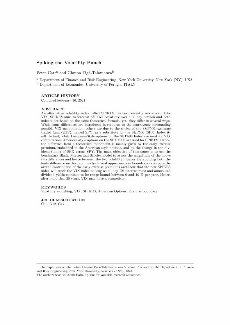
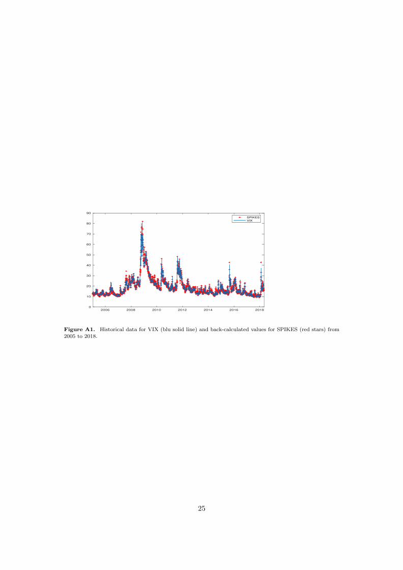
An analysis of data from 2005 to 2018 shows that the inclusion of the early exercisepremiums as well a the difference dividend timing in the SPIKES calculation has had anegligible impact on the average historical level of SPIKES, as evidenced in Figure A1,where both the historical values for VIX and the back-calculated values for SPIKESare plotted. It is clear from the picture that SPIKES tracks VIX during the wholeperiod. The simplest explanation for this negligible difference is that all of the optionsused in the volatility index calculations are OTM, hence with a small EEP. It alsohelps that US interest rates have averaged lower in this period than they did in thelate 1970’s, when inflation was larger. It is possible that a return of higher interestrates or a sharp increase in dividend payouts would increase the gap between SPIKESand VIX.

[Figure 1 about here.]

Table A1 reports some basic statistics for SPIKES and VIX levels and percentage log-differences (returns). The mean level of SPIKES at 18.90 has been slightly higher thanthat of VIX at 18.70; however, a two sample t-test cannot reject the null hypothesisof equal mean between the two time series, with a p-value of 0.34. The two volatil-ity indices also have very similar standard deviations and skewness. The percentagechanges in the two volatility indices are virtually indistinguishable over daily, weekly,and monthly horizons. This is confirmed, once again, by the outcomes of a t-test forwhich the null of equal means cannot be rejected at all frequencies. In addition, thetwo volatility indices have very similar, strongly negative correlations to the S&P 500over the daily, weakly and monthly horizons. Moreover, the correlation between bothlevels and percentage changes in the two volatility indices is nearly 1.

[Table 1 about here.]

As reported in Table A2, when SPIKES log-differences are regressed on VIX log-differences with no intercept, the estimated slope as well as the R2 of the regressionare both very close to 1. This result holds for daily, weekly, and monthly horizons. Thetable also shows the result of regressing SPY on SPX after adjusting for the differentdividend payout times:


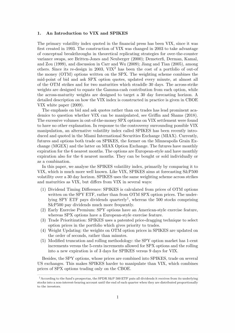
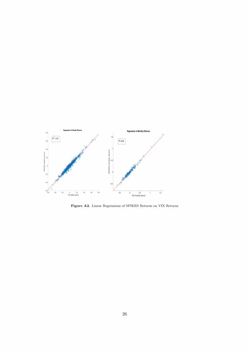
In Figure A2, the regression fit of SPIKES returns on VIX returns is plotted forweekly and monthly log-differences and confirm that the two indices have moved to-gether.


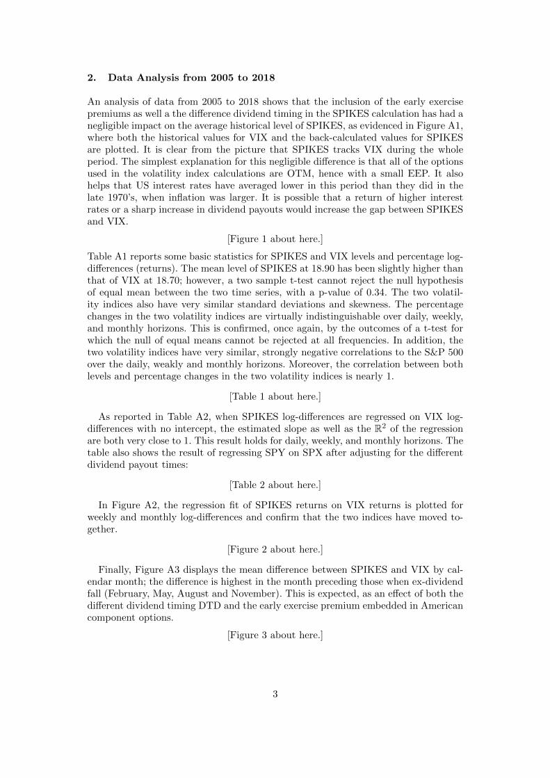
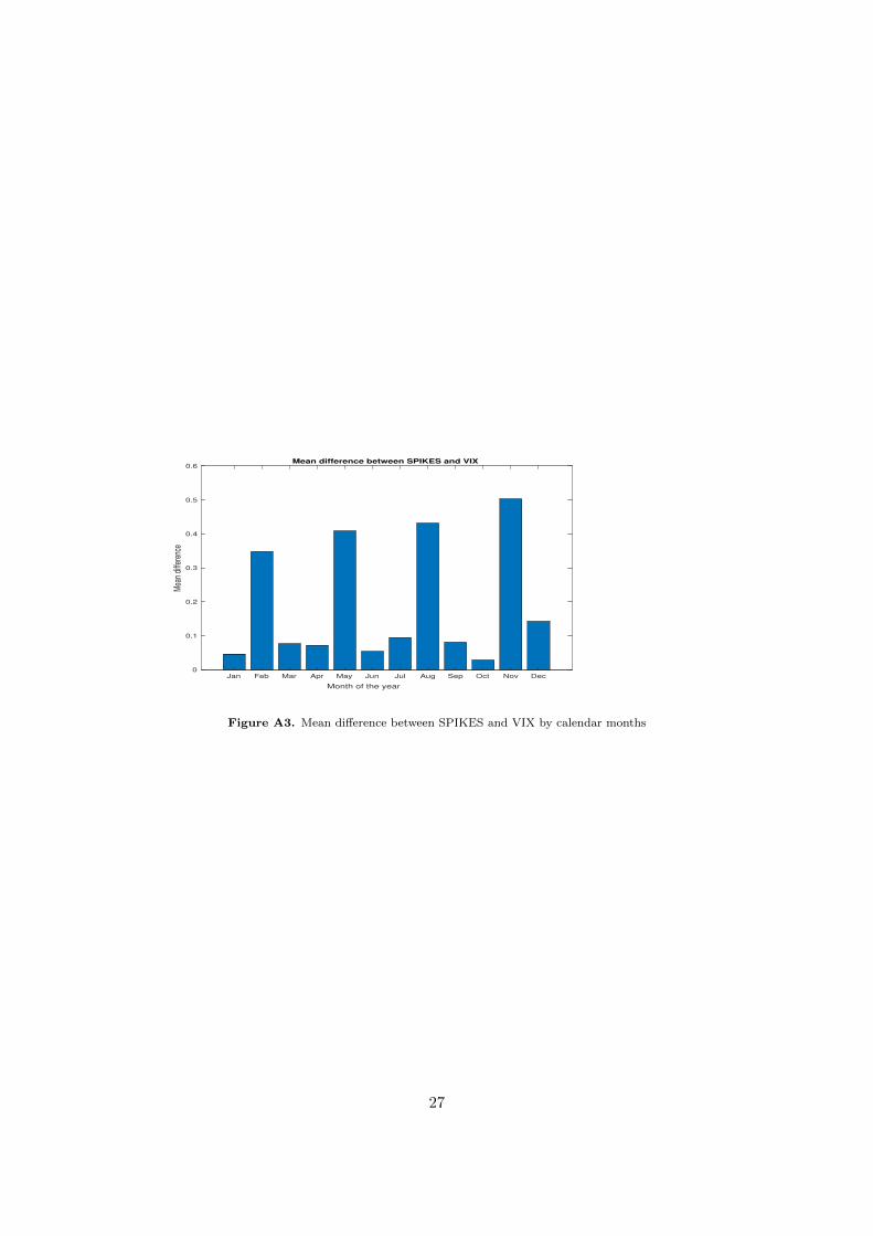
Finally, Figure A3 displays the mean difference between SPIKES and VIX by cal-endar month; the difference is highest in the month preceding those when ex-dividendfall (February, May, August and November). This is expected, as an effect of both thedifferent dividend timing DTD and the early exercise premium embedded in Americancomponent options.


3

3. Computing VIX, SPIKES and their difference

The computation of both SPIKES and VIX is based on a theoretical result for repli-cating the payoff on a variance swap via a static position in OTM European-styleindex options combined with dynamic trading in futures written on their underly-ing index, Britten-Jones and Neuberger (2000); Demeterfi et al. (1999). To ease one’sunderstanding of the construction of the two volatility indices, we introduce two con-cepts called TV IX and TSPIKES which stand for theoretical VIX and theoreticalSPIKES respectively.

For TV IX2, the cost of the theoretical replicating portfolio is:

TV IX2 =365

30

1

B

[∫ f

0

2

K2p

p(Kp)dKp +

∫ ∞f

2

K2c

c(Kc)dKc

](1)

where 365/30 is an annualization factor based on calendar days, B is the price of azero coupon bond paying $1 in 30 days, and f is the 30 day forward price of theS&P500 index, which, in practice, is approximated by the futures price. In (1), p(Kp)and c(Kc) respectively denote market prices of 30 day European-style OTM puts andcalls written on the S&P500 Index struck at Kp ∈ [0, f ] and Kc > f respectively.

Assuming no frictions, deterministic interest rates, and a strictly positive and con-tinuous futures price process, TV IX2 is the cost of replicating a fictitious varianceswap paying the quadratic variation of the log futures price at maturity. Academicssometimes wrongly describe this replication strategy as model-free, but what theyshould be writing is that this replication is not as model-dependent as the standardapproach for replicating path-dependent derivatives. Under either stochastic interestrates and/or jumps in price and/or non-negative futures prices, the terminal quadraticvariation of the log futures price cannot be theoretically replicated without further as-sumptions.

The magnitude of the variance swap replication failure increases as we move fromtheory towards practice, see Jiang and Tian (2007) for a comprehensive discussion.In practice, the actual variance swap has discrete monitoring, most often daily, andoften squares discrete time log price relatives of SPX, not its futures price. Sinceoption prices are only observed at discrete strikes, the above TV IX2 integral formulahas to be approximated by either fitting an implied volatility smile across strikes orby replacing the integral with a sum arising from truncation and discrete spacing ofstrikes. When a sum is used, a correction term needs to be added to capture the factthat f does not fall on a strike. Since observed option maturities are only rarely exactly30 days, a further approximation error is introduced by the necessity of interpolatingacross two maturities straddling 30 days. When:

• the annualization factor is based on minutes rather than days• the integral is replaced by a sum with a correction term• the maturity interpolation is linear

then the approximation of TV IX2 is called VIX2. As an aside, one can developboth a theory and a target ”variance swap like” payoff such that VIX2, ignoringthe correction term mentioned above, is the exact replication cost, as opposed to anapproximation of the replication cost of a theoretical or exact variance swap.TSPIKES is based on the same theoretical formula and weighting scheme as

TV IX, but where European-style options on the S& P500 Index (SPX) are nec-

4

essarily replaced by American-style options on the S& P500 ETF (SPY). Hence:

TSPIKES2 =365

30

1

B

[∫ F

0

2

K2p

P (Kp)dKp +

∫ ∞F

2

K2c

C(Kc)dKc

](2)

where P (Kp) and C(Kc) respectively denote market prices of the American-style OTMputs and calls written on the SPY ETF, struck at Kp ∈ [0, F ] and Kc > F respectively,and F is the 30 day forward price of the SPY ETF. However, unlike with TV IX2,there is no known theory under which TSPIKES2 is the initial cost of replicating atheoretical variance swap.

As for TV IX, the TSPIKES integral formula can also be approximated in prac-tice by an annualization factor, by truncation and discrete spacing of strikes, and bylinear interpolation across two maturities straddling 30 days. This approximation ofTSPIKES2 is called SPIKES2.

In variance swap replication theory, the market prices of the European optionsare observed directly. As a result, the only role of the underlying forward price is toseparate OTM Put strikes from OTM Call strikes. The underlying forward price is notneeded to calculate option premia from a model as the option premia are supposedto be directly observed. Likewise, the American option premia in TSPIKES aresupposed to be directly observed. In fact, when future values of SPIKES are to becompared to future values of VIX, we don’t observe future prices of the componentoptions. However, we can use an option pricing model to project these future optionprices onto future relevant stochastic state variables such as spot SPX or SPY, and/oran ATM implied volatility of SPX or SPY. We can then use the model to comparefuture levels of SPIKES to future levels of VIX, conditional on given numerical valuesof the relevant state variables.

When an American option on SPY is exercised early or at maturity, its payoff relatesto the spot value of SPY, not its futures price. When option pricing models are used todetermine the early exercise premium of a SPY option, it is easier to evolve the singlespot price of the underlying rather than to evolve the entire term structure of forwardor futures prices. It is also easier to assume that implied volatilities are constant acrossmoneyness and calendar time rather than to assume they vary with moneyness andstochastically over time.

If we assume that the only relevant stochastic state variable is the spot and that ithas constant proportional carrying costs and constant instantaneous volatility overtime, we are sing the BMS model to price options. Consider first the pricing ofEuropean-style SPX options; we assume for the rest of the paper that the dividendsfrom the 500 stocks in SPX are continuously paid over time and that the annualiseddividend yield of SPX is constant at some known level γ ≥ 0. In BMS setting therisk-free interest rate and the volatility are also constant at some known levels r andσ > 0 and so it is the proportional carrying cost r−γ ∈ R. Then the value of TV IX2,when the current value of the underlying SPX is at some known level X > 0, is givenby:

TV IX2 =365

30

1

B

[∫ f

0

2

K2p

pbs(X, γ,Kp)dKp +

∫ ∞f

2

K2c

cbs(X, γ,Kc)dKc

], (3)

where pbs(X, γ,Kp) and cbs(X, γ,Kc) respectively denote the BMS model value of aEuropean Put and Call for strikes Kp ∈ [0, f ] and Kc ≥ f respectively, f being the

5

forward price in T of the underlying SPX.Note that TV IX2 is independent of the inputs X, γ, r, and T that enter into the

relative pricing of each constituent SPX option and, in BMS model, is simply theconstant instantaneous variance rate σ2. However, when we move from TV IX2 toVIX2, VIX2 gains dependence on X, γ, r, and T due to the discreteness of strikes.

The theoretical counterpart of squared SPIKES, i.e. TSPIKES2, is defined by:

TSPIKES2 =365

30

1

B

[∫ F

0

2

K2p

P bs(Y, q,Kp)dKp +

∫ ∞F

2

K2c

Cbs(Y, q,Kc)dKc

](4)

where P bs(Y, q,Kp) and Cbs(Y, q,Kc) respectively denote the BMS model value of anAmerican Put and Call when SPY is at Y > 0, with constant quarterly paid dividendyield q ≥ 0, and for strikes Kp ∈ [0, F ] and Kc ≥ F respectively, F being the forwardprice of SPY.

Let (p/c)bs(Y, q,K) be the theoretical value of a European Put or Call on SPY.Suppose we subtract and add (p/c)bs(Y, q,K) in (4). Then we can decompose thedifference between TSPIKES2 and TV IX2 into two parts:

TSPIKES2 − TV IX2 = εx(Y, q) + δd(X,Y ; γ, q), (5)

where εx(Y, q) is the non-negative SPY option aggregate early exercise premium

εx(Y, q) =365

30

1

B

[∫ F

0

2

K2p

[P bs(Y, q,Kp)− pbs(Y, q,Kp)]dKp

+

∫ ∞F

2

K2c

[Cbs(Y, q,Kc)− cbs(Y, q,Kc)]dKc

]and δd(X,Y ; γ, q) the dividend timing difference :

δd(X,Y ; γ, q) =365

30

1

B

[∫ F

0

2

K2p

pbs(Y, q,Kp)dKp

+

∫ ∞F

2

K2c

cbs(Y, q,Kc)dKc

]− TV IX2.

Note that while the decomposition in (5) is model free the computation of the twoaddends depends on the assumption on the underlying assets X and Y . It is impor-tant to display the theoretical relationship between the two underlying assets SPXand SPY, with SPX having a constant continuously-paid, continuously-compounded,annualised dividend yield γ ≥ 0 and SPY having a constant quarterly-paid, quarterly-compounded annualised dividend rate q ≥ 0. Consider the one year price relatives X1

X0

and Y1

Y0when time 0 is just after SPY has paid a quarterly dividend. Let D0 be the

price at this time of a pure discount bond paying $1 in 1 year. Under the forward

measure Q1, we have D0EQ1

0X1

X0= e−γ , while D0E

Q1

0Y1

Y0=(

11+q/4

)4. Equating the two

expressions and solving for q one gets q = 4(eγ/4 − 1). Notice that q ≥ γ since the γis compounded more often.

6

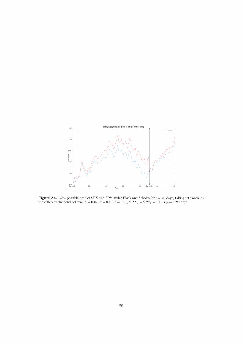
Under our model assumptions, it is possible to show that Yt =Xt exp (γ(t− TD(t))+) where TD(t) is the dividend date just before time t ≥ 0and Xt and Yt coincide at any ex-dividend date, just after the discrete dividend ispaid. In Figure A4, we plot an example of a price path for Y and X to illustrate thejump effect of the difference in the dividend schemes on the price dynamics. The Div-idend Timing Difference is due to the jump, possibly occurring due to a dividend datewithin the one-month time horizon, the magnitude of which can be expressed, underour assumptions, as a function of the proportional dividend rate q (Carr and Wu, 2009;

Klassen, 2009). Precisely, we have δd(X,Y ; γ, q) = δd(γ, q) = 2[log(1 + q

4

)− q/4

1+q/4

].


The overall contribution εx(Y, q) to the difference between TSPIKES2 and TV IX2,as indicated in (5), is obtained by adding the total EEPs arising from the Americancalls and American Puts. Specifically we can write:

εx(Y, q) = TotalEEPput + TotalEEPcall, (6)

where TotalEEPput, T otalEEPcall denote the aggregate contribution of Puts andCalls, respectively. The total contribution by Calls TotalEEPcall can be computedexplicitly. Since the SPIKES index is based on a 30 day horizon, there can be at mostone quarterly dividend payment from the underlying SPY ETF; when no dividend isexpected during the lifetime of the options (this happening overall in 2

3 of the days in ayear) this contribution vanishes while when one proportional dividend is expected, theEEP of an American-style Call is given, in the BMS setting, by the EEP of a Bermu-dan Option with exercise times TD, T and can be computed in closed form (Villiger,2006). The cumulative contribution TotalEEPcall is then obtained by simple integra-tion. Hence, in what follows we will focus on the computation of TotalEEPput. To thisend we develop an explicit approximation for the individual EEP of an American-stylePut which, suitably integrated, leads to an explicit formula for its weighted integralTotalEEPput. As a byproduct we obtain the pricing formula of an American put op-tions on an underlying paying discrete dividends in a BMS setting, thus complementingthe outcomes in Villiger (2006) which hold for American calls.

4. Closed form approximation for the Early Exercise Premium of anAmerican-style Put option

The underlying dynamics in Black and Scholes (1973) model can be generalised to thecase when the risky asset pays a single proportional dividend before maturity; if thecontinuously compounded interest rate is constant at r > 0 and Yt is the spot price attime t, representing the price of the underlying SPY, the dynamics of the process Yunder the risk-neutral probability measure Q, in t ∈ [0, T ], is given by:

dYt = rYtdt+ σYtdWt − δ(t− TD)Dtdt (7)

where Dt = qYt, q is the (annualised) proportional dividend rate and δ is the Diracdelta function. As already remarked, if the underlying stock pays no dividends be-tween the valuation time t and the option’s maturity date T , then an American Callwith expiration date T and strike price K has the same price as a European one

7

i.e. C(t, T,K) = c(t, T,K), where C and c denote the price of an American and aEuropean Call respectively. In contrast, American puts have a positive early exercisepremium.

4.1. The individual Early Exercise Premium

It is well known, see Carr, Jarrow, and Myneni (1992), that the initial value of anAmerican put’s EEP with expiry T , strike price K, and a non-dividend paying under-lying priced at Y0, may be represented as:

EEP (0, T,K) = EQ[rK

∫ T

0e−rt1{Yt<B(t,K)}dt

], (8)

where B(t,K) is the early exercise boundary for strike K and maturity T , which hasno known exact formula, but solves an integral equation. Precisely, under Black andScholes (1973) assumptions, Carr et al. (1992) proved that

EEP (0, T,K) = rK

∫ T

0e−rtN

ln(B(t,K)Y0

)−(r − σ2/2

)t

σ√t

dt. (9)

Indeed, the discrete nature of the dividend makes it possible to split the integral in(8) and write the early exercise premium for an American put as:

EEP (0, T,K) = EQ[rK

∫ TD

0e−rt1{Y ct <B(t,K)}dt+ rK

∫ T

TD

e−rt1{Y xt <B(t,T )}dt

](10)

= EQ[rK

∫ TD

0e−rt1{Y ct <B(t,T )}dt

]+ e−rTDEQ

[rK

∫ T

TD

e−r(t−TD)1{Y xt <B(t,T )}dt

],

where the cum-dividend stock price Y c appears in the indicator function in the firstintegral, while the ex-dividend stock price Y x appears in the indicator function in thesecond integral.

Theoretically, increasing the level of the short interest rate r raises each Americanput’s EEP, after accounting for the increase in the early exercise boundary B(t,K), t ∈[0, T ]. As a result, the overall effect of an increase in the interest rate r on the EEPshould be positive. The magnitude of this effect is obtained by computing the aboveintegrals, once we have some expression for the early exercise boundary B(t,K).

We assume that the early exercise boundary B(t,K), t ∈ [0, T ] is approximated byan exponential function of time, as in Ju (1998), both before and after the ex dividenddate. Precisely, the true early exercise boundary is approximated by Yp = {Yp(t), 0 <t < T}, defined as:

8

Yp(t) ≈

Ce−ht, if 0 < t < TD

Legt, if TD < t < T(11)

where C,L, h, g are positive constants.

Theorem 4.1. Assume we are under the MS model setting and that:

a1. the price changes of the risky asset Y in the time interval [0, T ] are described bythe dynamics in (7) with constant parameters r, σ, q and 0 < TD < T ;

a2. the early exercise boundary for American put options is approximated by the piece-wise exponential function in (11).

Then the early exercise premium for an American put with strike K and expirationdate T is approximated by

EEP (0, T,K) = f(Y c0 ;C,−h)− e−rTDEQ

[f(Y c

TDehTD ;C,−h)

](12)

+ e−rTDEQ[f(Y x

TDe−gTd ;L, g)

]− e−rTEQ

[f(Y x

T e−gT ;L, g)

],

with f : R3+ → R+ defined as:

f(y; l, u) =2rK

σ2(p+ − p−)

[1{y<l}

(1

p+− 1

p−− 1

p+

(y

l

)p+)− 1{y>l}

1

p−

(y

l

)p−],

(13)

where y = y exp (−ut) and p+, p− are the roots of P(p) = σ2

2 p2 + (r − u− σ2

2 )p− r.

Proof. A detailed proof is given in the Appendix.

Note that expected values are calculated using the cum-dividend initial price forthe first two terms and the ex-dividend price for the following others. The relevance ofthe above theorem is in the fact that the function f is not path dependent; while theLHS of the expression in (A15) depends on the distribution of the whole path from0 to T of the stochastic process Y , the RHS only depends, through f on the randomvariables YTD , YT . Further, it is straightforward to show that

Lemma 4.2. Under the assumptions of Theorem 4.1, if no dividends are due in [t, T ]then we have:

EQt[e−r(T−t)f(YT ; l, u)

]= Ke−r(T−t)N

(−d2(t, Yt, l, T )

)(14)

− 2rK

σ2(p+ − p−)

1

p+

(Ytl

)p+N(−d+

2 (t, Yt, l, T ))

− 2rK

σ2(p+ − p−)

1

p−

(Ytl

)p−N(d−2 (t, Yt, l, T )

)

9

where Yt = Y exp (−ut), d−2 (t, Yt, l, T ) = d2(t, Yt, l, T ) + p−σ√T − t and

d+2 (t, Yt, l, T ) = d2(t, Yt, l, T ) + p+σ

√T − t and Et denotes conditional expectation at

time t.

Proof. The proof is straightforward, given the known dynamics of the process Y and

observing that 2rσ2(p+−p−)

(1p+− 1

p−

)= 1.

It is worth to remark that the EEP in 4.1 can be computed explicitly by applyingLemma 4.2 where Y is replaced by either the cum-dividend process Y c or the ex-dividend process Yx. In this latter case the conditional expectation in t = TD iscomputed first and the unconditional expectation is obtained then by using the towerrule.

In order to gauge the magnitude of the approximation error, we solve the partial dif-ferential equation (PDE) obtained from the dynamics in (7) for a discrete proportionaldividend, q Y at TD, see also Gottsche and Vellekoop (2011). Notably, by applying fi-nite difference method to numerically solve the PDEs it is possible to get both theprice of American options and the (true) early exercise boundary. In Figures A5 andA6, we plot the (true) early exercise boundary obtained by numerical integration, forseveral values of the risk free rate r and the annualised dividend rate q, respectively.Indeed, the presence of a discrete dividend makes the boundary jump upward at timeTD which is decreasing in calendar time t before time TD, and increasing afterwards.In Figure A7 we plot both the true and the approximated boundary for a specificexample example with r = 2%, q = 3%,TD = 1/2 months and K = 100, T = 1 month.The exponential approximation is above the true so the closed form for the put optionEEP is an upward biased approximation of the actual one.




Figures A8 and A9, represent a zoom on the early exercise boundary respectivelyfor the period before and after the dividend date. In this pictures we also plot thelinear approximations obtained as steps towards the final exponential approximationof the boundary; the precise computation is detailed in the Appendix.



4.2. The cumulative Early Exercise Premium

The representation of the EEP of a single American put given in (13) allows us tocompute directly the excess of TSPIKES2 over TV IX2 arising from the early exercisepremium of component put options by integrating over all of the OTM strikes K ∈[0, F ], i.e. Total EEPPut(0, T ) =

∫ F0

2K2 EEP (0, T,K)dK. It is possible to prove the

following result:

10

Proposition 4.3. Under the assumptions of Theorem 4.1 the cumulative contributionof the early exercise premiums of OTM Puts is approximated by:

Total EEPPut(0, T ) = G(Y c0 ; a,−h)− e−rTDEQ

[G(Y c

TD ; a,−h)]

(15)

+ e−rTDEQ[G(Y x

t ; b, g)]− e−r(T )EQ

[G(Y x

T ; b, g)]

where Y cs = Y c

s exp (hs), Y xs = Y x

t exp (−gs), s ≥ 0 and a := C/K, b := L/K arepositive constants. Finally, the function G : R3

+ → R+ is defined as:

G(y; v, u) =4r

σ2(p+ − p−)(16)

×

[1{y<vF}

((1

p+− 1

p−

)log

Fv

y+

1

(p+)2

(yp

+

(Fv)p+− 1

)+

1

(p−)2

)+ 1{y>vF}

yp−

(vF )p−

],

where F is the forward price of the underlying Y for maturity T , y = y exp (−ut) and

p+, p− are the roots of P(p) = σ2

2 p2 + (r − u− σ2

2 )p− r.

Proof. It suffices to compute the following integral:

G(y, v, u) =

∫ F

0

2

K2f(y, vK, u)dK

=

∫ F

0

2

K2

2rK

σ2(p+ − p−)

(1{y<vK}

(1

p+− 1

p−− 1

p+

yp+

(vK)p+

)− 1{y>vK}

1

p−yp

−

vKp−

)dK

=4r

σ2(p+ − p−)×∫ F

0

1

K

(1{y<vK}

(1

p+− 1

p−− 1

p+

yp+

(vK)p+

)− 1{y>vK}

1

p−yp

−

vKp−

)dK

Since all the addends in the integrating function are power functions in K, the finalexpression for G is obtained by applying elementary integration rules.

The Total EEP can be approximated by a closed formula since the expectationsappearing in (16) can be computed explicitly.

Lemma 4.4. Under the assumptions of Theorem 4.1, if no dividends are due in [t, T ]then we have:

EQt[e−r(T−t)G(YT ; v, u)

]= 2e−rt

[(log

Feu(T−t)v

Yt(1− q)er−σ2/2− 2r

σ2(p+ − p−)

(1

(p+)2− 1

(p−)2

))(17)

×N(−d2(t, T, Yt(1− q), Fveut)

)+ σ√tN ′(−d2(t, T, Yt(1− q), Fveut)

)]+

4r

σ2(p+ − p−)

1

(p+)2

(Yt(1− q)Fv

)p+N(−d2(t, T, Yt(1− q), Fveu(T−t))− σp+

√T − t

)+

4r

σ2(p+ − p−)

1

(p−)2

(Yt(1− q)Fv

)p−N(d2(t, T, Yt(1− q), Fveu(T−t))+σp−

√T − t

).

11

where F is the forward price of the underlying Y prevailing at time t for maturityT , Yt = Y exp (−ut), d−2 (t, Yt, l, T ) = d2(t, Yt, l, T ) + p−σ

√T − t and d+

2 (t, Yt, l, T ) =

d2(t, Yt, l, T ) + p+σ√T − t and Et denotes conditional expectation at time t.

Proof. The proof is straightforward, given the known dynamics of the process Y in

BMS setting and observing that 2rσ2(p+−p−)

(1p+− 1

p−

)= 1.

We remark that when there is no dividend paid during the lifetime of SPY options,then the overall contribution of puts to the EEP reduces to:

Total EEPPut(0, T ) = G(Y0, b, g)− e−r(T )EQ[G(YT , b, g)

]. (18)

5. Numerical Results

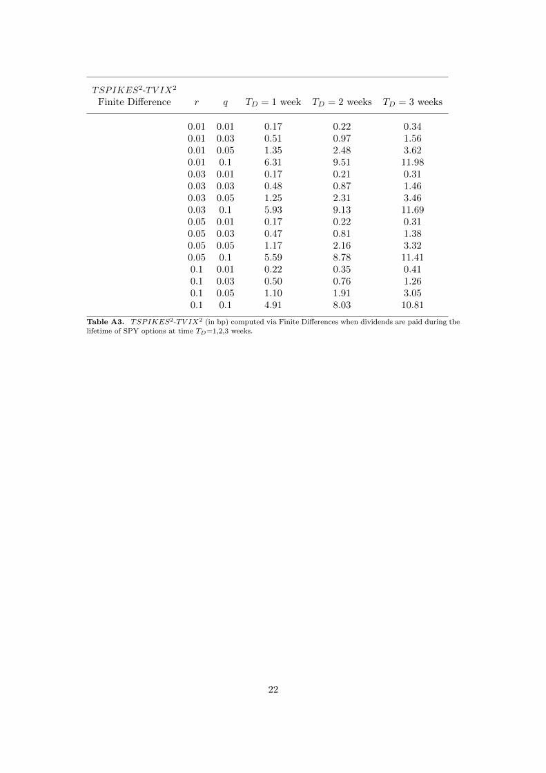
In this section, we derive the difference between TSPIKES2 and TV IX2 by comput-ing the early exercise premiums for American call and put components via a Crank-Nicolson finite difference scheme. We consider different examples for which the divi-dend is paid one week, two weeks and three weeks ahead, with option expiring in onemonth for both SPY and SPX options. For each case, we fix Y0 = 100, σ = 0.2, andT = one month. We let r and q vary to test how interest rates and dividend yields affectthe difference between SPIKES2 and V IX2. The numerical integration to obtain thetwo volatility indices is truncated at Klowest = 30 for the puts and Khighest = 200 forthe calls. The above difference is then compared with the closed form approximationobtained by adding three terms: the exact Dividend Timing Difference (DTD), theexact contribution of calls to the total EEP, and the total contributions of puts to theEEP, obtained by applying Proposition 4.3 and Lemma4.4.

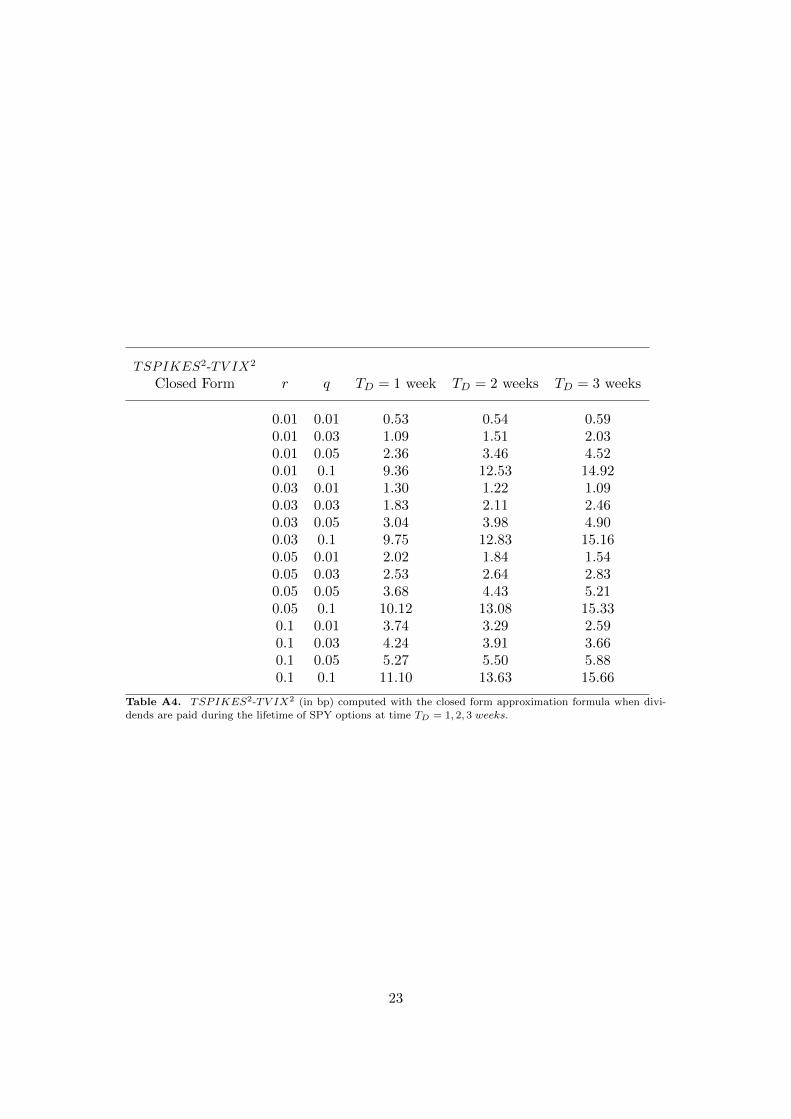
In Table A3 and Table A4, we report the value in basis points of the total differencebetween (truncated) TSPIKES2 and TV IX2 for several pairs of r and q.


It is clear from Table A3 that the true difference between TSPIKES2-TV IX2 isnegligible. We draw the same qualitative conclusion from the outcomes displayed inTable A4, obtained by applying the closed formulas. As expected the approximationis upward biased and the error is between 0.25 and 6 basis points for the consideredexamples. For any pair of interest and dividend rate the difference increases whenthe dividend date gets closer to this expiration date, as expected from the theoreticaldiscussion an consistently with Figure A3.


One naturally wonders whether OTM calls or OTM puts are more important inexplaining the cumulative EEP across strikes, contributing to the difference betweenTV IX2 and TSPIKES2. In order to answer to this question we report in Table A5,the separate contributions of OTM calls and OTM puts to the total EEP, computed byapplying the closed formulas, for the example case when a single dividend is paid duringSPY options lifetime in TD = 3 weeks. The total contribution of calls is increasingin the dividend rate q and decreasing in the interest rate and, as expected, the totalcontribution of Puts does not vary with q and it is increasing with r; the dividend

12

timing difference is increasing in q and does not change with r. Overall, the impact ofa change in the dividend rate is higher than that in the interest rate.


6. Conclusions and Future Research

When SPIKES is back-calculated to 2005, it hardly differs from VIX. We used thebenchmark BMS model to discuss the main causes of this difference and to asseswhether it would remain negligible in other scenarios. In order to prove this results wedecomposed the difference between the theoretical counterparts of the two indexes intwo main terms: the dividend timing difference and the total early exercise premium.The former is due to the different dividend payment scheme for SPX and SPY whichare the underlying assets of the constituent options, respectively for VIX and SPIKESand it is shown to be only dependent on the value of the annualised dividend rateq. The latter gathers the early exercise premiums arising from the American exercisestyle of SPY options against the European style of SPX options. The contribution ofcalls can be computed in close form by applying the outcomes in Villiger (2006); wederive in this paper an analogous closed form expression for the early exercise of a putoptions and for the aggregate contribution of Put option on SPIKES. In the numericalillustration we show that the new SPIKES index will continue tracking the VIX indexas long as 30 day US interest rates and annualised dividend yields continue to be rangebound between 0 and 10 % per year and we compare the (true) difference computedby applied the finite difference method to solve the model PDE with the closed formapproximations proposed in this paper. We did not consider negative interest ratesin the numerical application; indeed, both VIX and SPIKES are quoted in UnitedStates where interest rates have remained positive to date and, most likely, shouldstay positive in the future. Even during the recent pandemic the US Fed has refrainedfrom pushing its benchmark rates below zero. Anyway, the theory tells us that in caseof negative interest rates the contribution of American Calls to the total early exercisepremium would increase as it may become convenient, under such circumstances, toexercise a call before its expiration. However, Puts would never be exercised early andthe contribution of American puts to the early exercise premium would vanish. Hence,we don’t expect substantial changes to the overall difference between TSPIKES andTV IX if the interest rate r was assumed negative. We have also evidenced how theimpact of the dividend rate is higher than that of the interest rate, affecting both thedividend timing difference and the total EEP from Calls. Notably, during the historicalperiod analysed in this paper dividend rates for the SPY ETF have remained around2% but for a single peak at 3.3%, as illustrated in Figure A10. Overall, we expect thegap between SPIKES and VIX to increase substantially only in case of an extremelypositive performance of the stocks underlying the SPY ETF.


It is worth noticing that we also believe the prices of the near and next maturityOTM options used to calculate both SPIKES and VIX respond primarily to volatility,along with interest rates and dividends. Future research can investigate whether thesensitivity of TSPIKES2 and TV IX2 with respect to the volatility parameter σdiffers substantially, in line with the approach in Demeterfi et al. (1999). Given (5), itsuffices to compute the derivative of the total EEP εx(Y, q) with respect to σ. This is

13

easily approximated in closed form by computing the corresponding derivative of theexpressions for the Total EEP for Calls, available by applying the outcomes in Villiger(2006) and that of the Total EEP for Puts given in (16), when a discrete dividend ispaid by the SPY ETF during the lifetime of the options. When no dividends are paidby the SPY ETF before expiration, Vega is calculated by differentiating the expressionin (18) with respect to σ. Preliminary results indicate that the numerical differencebetween the two Vegas is small, but not always negligible.

It is also worth to investigate whether these initial conclusions are robust to theassumptions that interest rates, dividend yields, and variance rates are constant. Whenall three of these rates are allowed to be stochastic, the extra optionality in an Americanoption gives its holder the right to swap an exposure based primarily on volatility for aswap between interest and dividends. The EEP should rise due to this extra volatilityvalue and so should the gap between SPIKES and VIX. We leave this analysis tofuture research.

Funding

Gianna Figa-Talamanca was the recipient of research mobility funds from the Uni-versity of Perugia during the preparation of this paper. The H2CU center is alsoacknowledged for indirect funding.

References

Bekaert G, Hoerova M (2014) The vix, the variance premium and stock market volatility.Journal of econometrics 183(2):181–192

Black F, Scholes M (1973) The pricing of options and corporate liabilities. Journal of politicaleconomy 81(3):637–654

Britten-Jones M, Neuberger A (2000) Option prices, implied price processes, and stochasticvolatility. The journal of Finance 55(2):839–866

Carr P, Wu L (2009) Variance risk premiums. The Review of Financial Studies 22(3):1311–1341Carr P, Jarrow R, Myneni R (1992) Alternative characterizations of american put options.

Mathematical Finance 2(2):87–106Demeterfi K, Derman E, Kamal M, Zou J (1999) More than you ever wanted to know about

volatility swaps. Goldman Sachs quantitative strategies research notes 41:1–56Gottsche O, Vellekoop M (2011) The early exercise premium for the american put under dis-

crete dividends. Mathematical Finance: An International Journal of Mathematics, Statisticsand Financial Economics 21(2):335–354

Griffin JM, Shams A (2018) Manipulation in the vix? The Review of Financial Studies31(4):1377–1417

Jiang GJ, Tian YS (2005) The model-free implied volatility and its information content. TheReview of Financial Studies 18(4):1305–1342

Jiang GJ, Tian YS (2007) Extracting model-free volatility from option prices: An examinationof the vix index. The Journal of Derivatives 14(3):35–60

Ju N (1998) Pricing by american option by approximating its early exercise boundary as amultipiece exponential function. The Review of Financial Studies 11(3):627–646

Klassen T (2009) Pricing variance swaps with cash dividends. Wilmott Journal: The Interna-tional Journal of Innovative Quantitative Finance Research 1(4):173–177

CBOE VIX white paper CBOE (2009) The cboe volatility index–vix. White paperVilliger R (2006) Valuation of american call options. Wilmott magazine 3:64–67

14

Appendix A. Proof of Theorem 4.1.

In this appendix we develop the necessary steps in order to approximate the exerciseboundary and hence the EEP for the American-style Put options considered in theSPIKES Index computation. These are written on an underlying paying a single dis-crete proportional dividend qY at the dividend date TD < T , being T their expirationdate. It is worth noticing that the dividend date plays a crucial role in the approxima-tion of the early exercise boundary for the options, which jumps at time TD. Indeed,after time TD, the option reduces to an American Put written on a non-dividendpaying asset.

The proof is given by proceeding in steps:

(1) we restrict our attention to the time interval (TD, T ], where no dividends aredue, and consider a constant boundary L by setting g = 0 in (11).

(2) we apply a change of probability measure to derive a closed form formula whenthe exercise boundary is approximated by an exponentially growing boundary,g 6= 0, once again focusing on the time interval after the dividend date TD;

(3) we generalise the outcomes of previous steps for approximating the exerciseboundary and computing the EEP of an American-style Put for t < TD.

Note that in the first two steps we assume that the early exercise boundary is flatat the level 0 for t ≤ TD. This corresponds to approximating the price of the AmericanPut option with that of a hybrid American Put which can be exercised at any time in(TD, T ].

Step 1 Since there are no dividends in the time interval (TD, T ], the early exercisepremium for the hybrid put is just the present value of the interest earned on thestrike price, while the stock price is below the early exercise boundary, as shown inCarr et al. (1992), which we assume to be constant at L in the time interval (TD, T ].

Hence, the price PH at time t < TD of the hybrid put is given by:

PH(t, Yt, T,Kp;L) = p(t, Yt, T,Kp, L) (A1)

+ e−r(TD−t)EQ[rKp

∫ T

TD

e−r(u−TD)1{Yu<Yp(u)}du

]. (A2)

The critical stock price at time TD is defined as the level for Y such that the con-tinuation value of the hybrid put equals its exercise value; if we further assume thatthe exercise boundary is constant at this critical stock price after time TD, then Limplicitly solves:

PH(TD, L, T,K;L) = K − L. (A3)

We know that when the underlying asset is non-dividend paying, the value at times ∈ (TD, T ], of interest on the strike while Y < L is

EQs[rK

∫ T

se−r(u−s)1{Yu<L}du

]. (A4)

Consider a function f : R+ −→ R+ with f ∈ C2 . By applying Ito’s Lemma in

15

integral form we get

e−rT f(YT ) = f(Ys) +

∫ T

se−r(u−s)f ′(Yu)dYu

+

∫ T

se−r(u−s)[

f ′′(Yu)

2σ2Y 2

u − rf(Yu)]du

= f(Ys) +

∫ T

se−r(u−s)f ′(Yu)[dYu − rYudu]

+

∫ T

se−r(u−s)[

f ′′(Yu)

2σ2Y 2

u + rYuf′(Yu)− rf(Yu)]du

and, taking conditional expectation at time s we get,

e−r(T−s)EQs [f(YT )] = f(Ys)+EQs[∫ T

se−r(u−s)[

f ′′(Yu)

2σ2Y 2

u + rYuf′(Yu)− rf(Yu)]du

].

(A5)Hence, the value of the accrued interest on the strike for Y < L may be written, inTD as

EQTD

[rK

∫ T

TD

e−r(u−TD)1{Yu<L}du

]= f(YTD)− e−r(T−TD)EQTD [f(YT )] , (A6)

if and only if there exists a function f(Y ) solving the following ordinary differentialequation (ODE):

f ′′(Y )

2σ2Y 2 + rY f ′(Y )− rf(Y ) = −rK1{Y <L}. (A7)

It is straightforward to show that a solution exists for any constant L, and it isgiven by

f(Y ;L) =Kp

r + σ2

2

[1{Y <L}

(r +

σ2

2− rY

L

)+ 1{Y >L}

σ2

2

(Y

L

)−2r/σ2]. (A8)

The function f(Y ;L) can be seen as a final payoff at T whose time value at s matchesthe value of the interest earned on the strike price K when Y < L between s and T .Finally, by discounting and applying the tower property for conditional expectation,the price of the hybrid put with constant boundary at time t, for 0 ≤ t ≤ TD , is given

PH(t, Yt, T,Kp;L) = p(t, Yt, T,Kp) + e−r(TD−t)EQt[f(YTD ;L)− e−r(T−TD)f(YT ;L)

].

(A9)To solve for L, we must compute the above price at time TD i.e. conditioning on

the information available at time TD and then solve (A3). Note that we can writeL = bKp for some positive constant b.

16

The early exercise premium in TD for the hybrid put can be computed explicitly:

EEPH(TD, T,Kp) = EQTD[f(YTD ;L)− e−r(T−TD)f(YT ;L)

]=

Kp

r + σ2

2

[(r +

σ2

2)[1{YTD<L} − e

−r(T−TD)N (−d2 (TD, YTD , T, L))]

−rYTDL

[1{YTD<L} −N (−d1 (TD, YTD , T, L))

]]+

K

r + σ2

2

σ2

2

(YTDL

)−2r

σ2[1{YTD>L} −N

(d2 (TD, YTD , T, L)− 2r

σ

√T − TD

)].

(A10)

Finally, the early exercise premium at time t = 0 for the hybrid put is simply thediscounted value of the premium in A10:

EEPH(0, T,Kp) =

Kp

[e−rTDN (−d2 (0, Y0(1− q), TD, L))− e−r(T−TD)N (−d2 (0, Y0(1− q), T, L))

]− Kp

r + σ2

2

rY0(1− q)L

[N (−d1 (0, Y0(1− q), TD, L))−N (−d1 (0, Y0(1− q), T, L))]

+Kp

r + σ2

2

σ2

2

(Y0(1− q)

L

)−2r

σ2[N

(d2 (0, Y0(1− q), TD, L)− 2r

σ

√TD

)−N

(d2 (0, Y0(1− q), T, L)− 2r

σ

√T

)],

so the price at time t = 0 for the hybrid put is given by:

PH(0, Y0, T,Kp;L) = p(0, Y0, T,Kp) + EEPH(0, T,Kp). (A11)

Step 2As an improved approximation for the early exercise premium and the price of the

hybrid American option introduced above, we let the exponential growth coefficient gbe non-zero in (11). The boundary is again assumed to be flat at 0 before the dividenddate TD.

Several methods are available to obtain the constants L, g specifying the approxi-mating exponential function. Here, we obtain these constant imposing value matchingconditions at times TD and T , according to the outcomes in Ju (1998).

We extend the approach used in Step 2 and define a function f which representsthe payoff flow of the EEP in the time span (TD, T ].

Define the auxiliary process Yt := Yte−gt. Under the risk-neutral probability measure

Q, the price changes of Y are described by:

dYt = (r − g)Ytdt+ σYtdWt − δ(t− TD)Dtdt.

17

We can use a similar approach to that of a constant boundary and find a functionf such that

EQt[rKp

∫ T

te−r(u−t)1{Yu<L}du

]= f(Yt)− e−r(T−t)EQt

[f(YT )

], (A12)

which is obtained by solving:

f ′′(Y )

2σ2Y 2 + (r − g)Y f ′(Y )− rf(Y ) = −rK1{Y <L}. (A13)

The solution is:

f(Y ;L, g) =2rKp

σ2(p+ − p−)

[1{Y <L}

(1

p+− 1

p−− 1

p+

(Y

L

)p+)− 1{Y >L}

1

p−

(Y

L

)p−],

(A14)

where p+, p− are the roots of P(p) = σ2

2 p2 + (r − g − σ2

2 )p− r.Note that once this new function is computed, the case of an exponential boundary

for the underlying stock Y is equivalent to that of a constant boundary for the processY .

Hence, as in the previous subsection, we get

EEPH(TD, T,K) = EQTD[f(YTD)− e−r(T−TD)f(YT )

]=

2rKp

σ2(p+ − p−)

[(

1

p+− 1

p−)[1{YTD<L}

− e−r(T−TD)N(−d2

(TD, YTD , T, L

))]− 1

p+

(YTDL

)p+ [1{YTD<L}

−N(−d2

(TD, YTD , T, L

)− p+σ

√T − TD

)]]

− 2rKp

σ2(p+ − p−)

1

p−

(YTDL

)p− [1{YTD>L}

−N(d2

(TD, YTD , T, L

)+ p−σ

√T − TD

)],

and similarly we obtain the early premium at time t = 0 by computing its discountedvalue and the corresponding hybrid option price.

Step 3 We finally consider the case of an American option which can be exercisedthroughout its lifetime [0, T ]. This can be done by applying the outcomes obtained inStep 2 for different exponential approximating functions before and after the dividenddate TD, respectively as defined in (11) and considering the cum-dividend and theex.dividend process respectively. The challenge here is to obtain the constant valuesC, h for which we cannot apply the same method as above. By looking at Figures A5and A6, it is evident that the exercise boundary is essentially linear before time TDand vanishes at time TD. We want the exponential approximation before time TD toemulate the linear behaviour displayed by the true boundary computed numerically;since TD < T ≈ 1/12, this is easily achieved by setting the constant h in (11) to a smallvalue. Further, we surmise from the pictures that the intercept is approximately at thelevel r

qKTD. A linear boundary approximation with the above properties is given by

18

y = rqK(TD − t), which can be in turn approximated by an exponential function with

C = rqKTD and h = 1

TD. The linear boundary may also be calibrated by matching the

average slope of the area under the linear and exponential boundary approximations;the results are qualitative analogous. Once the values for C, h are computed, then theoverall early exercise premium for an American put with strike Kp and expiration dateT , can be computed by summing the two early exercise premiums for the first andsecond part of the approximated boundary. Precisely,

EEP (0, T,K) = f(Y c0 ;C, h)− e−rTDEQ

[f(Y c

TDehTD ;C, h)

](A15)

+ e−rTDEQ[f(Y x

TDe−gTD ;L, g)

]− e−rTEQ

[f(Y x

T e−gT ;L, g)

],

where the expected values are calculated using the cum-dividend initial price for thefirst two terms and the ex-dividend price for the others. This finally proves Theorem4.1. �

19

Statistics Index Daily Ret. Weekly Ret. Monthly Ret.

Vol. Index VIX, SPIKES VIX, SPIKES VIX, SPIKES VIX, SPIKESMean 18.70, 18.90 0.28%, 0.28% 1.1%, 1.1% 3.10%, 3.00%Std. Dev. 9.20, 9.20 123%, 123% 115%, 112% 96%, 94%Skewness 2.50, 2.50 2.20, 2.90 2.80, 2.80 2.70, 2.90SPX Corr. -51% , -50% -72%, -71% -71%, -71% -69%, -69%VIX Corr. 1, 99.9%, 1, 97.4%, 1, 98.5% 1, 99.1%

Table A1. Descriptive statistics for VIX, SPIKES and their returns from 2005 to 2018

20

Asset Pair Daily Return R2 Weekly Return R2 Monthly Return R2

SPIKES vs. VIX 0.95 0.97 0.98SPY vs. SPX 0.98 0.99 1.00

Table A2. The R2 value when SPIKES returns are regressed on VIX returns (top row) and SPY returns areregressed on SPX returns (bottom row).

21

TSPIKES2-TV IX2

Finite Difference r q TD = 1 week TD = 2 weeks TD = 3 weeks

0.01 0.01 0.17 0.22 0.340.01 0.03 0.51 0.97 1.560.01 0.05 1.35 2.48 3.620.01 0.1 6.31 9.51 11.980.03 0.01 0.17 0.21 0.310.03 0.03 0.48 0.87 1.460.03 0.05 1.25 2.31 3.460.03 0.1 5.93 9.13 11.690.05 0.01 0.17 0.22 0.310.05 0.03 0.47 0.81 1.380.05 0.05 1.17 2.16 3.320.05 0.1 5.59 8.78 11.410.1 0.01 0.22 0.35 0.410.1 0.03 0.50 0.76 1.260.1 0.05 1.10 1.91 3.050.1 0.1 4.91 8.03 10.81

Table A3. TSPIKES2-TV IX2 (in bp) computed via Finite Differences when dividends are paid during the

lifetime of SPY options at time TD=1,2,3 weeks.

22

TSPIKES2-TV IX2

Closed Form r q TD = 1 week TD = 2 weeks TD = 3 weeks

0.01 0.01 0.53 0.54 0.590.01 0.03 1.09 1.51 2.030.01 0.05 2.36 3.46 4.520.01 0.1 9.36 12.53 14.920.03 0.01 1.30 1.22 1.090.03 0.03 1.83 2.11 2.460.03 0.05 3.04 3.98 4.900.03 0.1 9.75 12.83 15.160.05 0.01 2.02 1.84 1.540.05 0.03 2.53 2.64 2.830.05 0.05 3.68 4.43 5.210.05 0.1 10.12 13.08 15.330.1 0.01 3.74 3.29 2.590.1 0.03 4.24 3.91 3.660.1 0.05 5.27 5.50 5.880.1 0.1 11.10 13.63 15.66

Table A4. TSPIKES2-TV IX2 (in bp) computed with the closed form approximation formula when divi-

dends are paid during the lifetime of SPY options at time TD = 1, 2, 3 weeks.

23

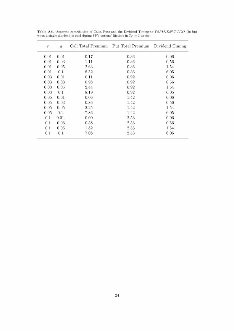
Table A5. Separate contribution of Calls, Puts and the Dividend Timing to TSPIKES2-TV IX2 (in bp)

when a single dividend is paid during SPY options’ lifetime in TD = 3 weeks.

r q Call Total Premium Put Total Premium Dividend Timing

0.01 0.01 0.17 0.36 0.060.01 0.03 1.11 0.36 0.560.01 0.05 2.63 0.36 1.540.01 0.1 8.52 0.36 6.050.03 0.01 0.11 0.92 0.060.03 0.03 0.98 0.92 0.560.03 0.05 2.44 0.92 1.540.03 0.1 8.19 0.92 6.050.05 0.01 0.06 1.42 0.060.05 0.03 0.86 1.42 0.560.05 0.05 2.25 1.42 1.540.05 0.1. 7.86 1.42 6.050.1 0.01. 0.00 2.53 0.060.1 0.03 0.58 2.53 0.560.1 0.05 1.82 2.53 1.540.1 0.1 7.08 2.53 6.05

24

2006 2008 2010 2012 2014 2016 2018

0

10

20

30

40

50

60

70

80

90

SPIKES

VIX

Figure A1. Historical data for VIX (blu solid line) and back-calculated values for SPIKES (red stars) from

2005 to 2018.

25

-0.6 -0.4 -0.2 0 0.2 0.4 0.6 0.8

VIX weekly returns

-0.6

-0.4

-0.2

0

0.2

0.4

0.6

0.8

SP

IKE

S w

eekly

retu

rns

Regression of Weekly Returns

R2 = 0.97

-0.5 0 0.5 1 1.5

VIX monthly returns

-0.5

0

0.5

1

1.5

SP

IKE

S m

on

thly

retu

rns

Regression of Monthly Returns

R2=0.98

Figure A2. Linear Regressions of SPIKES Returns on VIX Returns

26

Mean difference between SPIKES and VIX

Jan Feb Mar Apr May Jun Jul Aug Sep Oct Nov Dec

Month of the year

0

0.1

0.2

0.3

0.4

0.5

0.6

Mea

n di

ffere

nce

Figure A3. Mean difference between SPIKES and VIX by calendar months

27

Div. in t=0 20 40 60 80 Div. in t=90 100 120

Days

100

105

110

115

120

125

Underlyin

g P

rice

Underlyings dynamics acccording to different dividend timing.

Y

X

Figure A4. One possible path of SPX and SPY under Black and Scholes for n=120 days, taking into account

the different dividend scheme: γ = 0.02, σ = 0.20, r = 0.01, SPX0 = SPY0 = 100, TD = 0, 90 days.

28

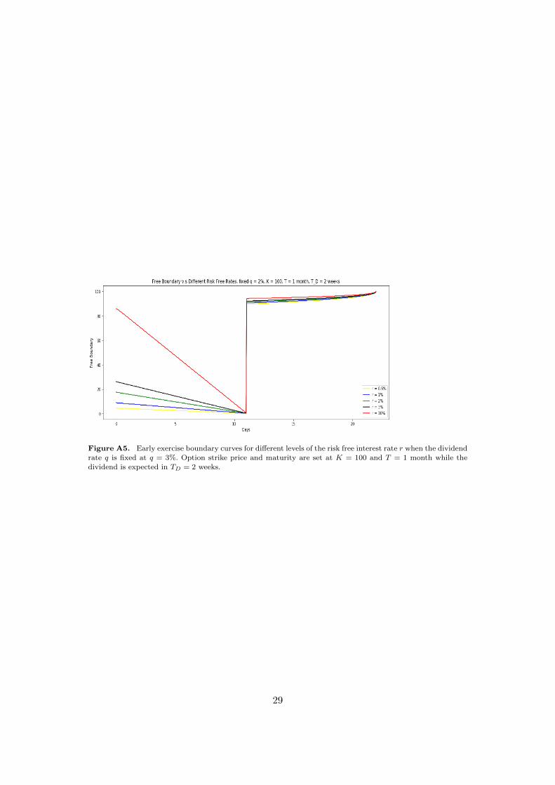
Figure A5. Early exercise boundary curves for different levels of the risk free interest rate r when the dividend

rate q is fixed at q = 3%. Option strike price and maturity are set at K = 100 and T = 1 month while thedividend is expected in TD = 2 weeks.

29

Figure A6. Early exercise boundary curves for different levels of the dividend rate q when the risk free

interest rate is fixed at r = 2%. Option strike price and maturity at fixed at K = 100 and T = 1 month whilethe dividend is expected in TD = 2 weeks.

30

Figure A7. Early exercise boundary curve when r = 2%. Option strike price and maturity are set at K = 100

and T = 1 month while the dividend is expected in TD = 2 weeks.

31

m

Figure A8. Early exercise boundary before the dividend date TD: Finite difference (Red), Linear approxi-mation (Green), Exponential approximation (Blue)

32

Figure A9. Early exercise boundary after the dividend date TD: Finite difference (Red), Constant approxi-mation (Green), Exponential approximation (Blue)

33

Figure A10. Historical values of the SPY dividend rate q from 2005 to 2018.

34

Documents

Spiking the Volatility Punch - New York University