Spiking Neurons and Synaptic Stimuli: Determining the ... · Abstract— Similarity between two spike trains is generally ... University of Hull, Hull, East-Yorkshire, HU6 7RX, UK

Abstract— Similarity between two spike trains is generally

estimated using a ‘coincidence factor’. This factor relies on

counting coincidences of firing-times for spikes in a given time

window. However, in cases where there are significant

fluctuations in membrane voltages, this uni-dimensional view is

not sufficient. Results in this paper show that a two-dimensional

approach taking both firing-time and the magnitude of spikes is

necessary to determine similarity between spike trains. It is

observed that the difference between the lower-bound limit of

faithful behaviour and the reference inter-spike interval (ISI)

reduces with the increase in the ISI of the input spike train. This

indicates that spike trains generated by two highly-varying

currents have a high coincidence factor thus indicating higher

similarity – a limitation imposed due to a one-dimensional

comparison approach. These results are analysed based on the

responses of a Hodgkin-Huxley neuron, where the synaptic

input induces fluctuations in the output membrane voltage. The

requirement for a two-dimensional analysis is further supported

by a clustering algorithm which differentiates between two

visually-distinct responses as opposed to coincidence-factor.

Index Terms—coincidence-factor, fluctuations, comparison,

synaptic stimuli, membrane voltage.

I. INTRODUCTION

The responses of a neuron to various types of stimuli have

been studied extensively over the past years [1]-[9].

Stimulus-dependent behaviour of neurons has already been

pursued to understand the spiking responses and it is thought

that either the firing rate or firing time of individual spikes

carries specific information of the neuronal response [3],

[10]-[16]. The response of the neurons studied above has a

constant magnitude whose variance is very low. In this paper,

the neural responses fluctuate and a one-dimensional analysis

based on firing times is shown to be insufficient for

comparison.

A supra-threshold static current stimulus is sufficient to

induce a spiking behaviour in the neuron. The magnitude of

these action potentials is considered to be almost the same and

Manuscript received October 13, 2008. Spiking Neurons and Synaptic

Stimuli: Determining the Fidelity of Coincidence-Factor in Neural Response

Comparison

Mayur Sarangdhar is currently a PhD student within the Neural,

Emergent and Agent Technologies Group, Department of Computer

Science, University of Hull, Hull, East-Yorkshire, HU6 7RX, UK (phone:

01482 465253; e-mail: M.Sarangdhar@ 2006.hull.ac.uk).

C. Kambhampati is currently a Reader in the Department of Computer

Science, University of Hull, Hull, East-Yorkshire, HU6 7RX, UK. (e-mail:

[email protected]).

their variance is thus ignored. Such responses have been

studied and models to depict their spiking behaviour have

been proposed and implemented [17]-[28]. On the other hand,

a synaptic current is used to stimulate the same neuron [3].

This synaptic current comprises of a static and a pulse

component and is of particular interest as it induces

fluctuations in the membrane voltage. These responses can be

compared by their firing times [18], [20], [23]-[26] using a

measure of comparison known as coincidence-factor. Here,

the generality of this approach is investigated for a

Hodgkin-Huxley (H-H) neuron [29] for which a synaptic

current induces membrane fluctuations.

In this paper, neural responses are generated by changing

the Inter-Spike-Interval (ISI) of the stimulus. These responses

are subsequently compared and a coincidence factor is

calculated. Coincidence-factor, a measure of similarity, is

expected to generate a high value for higher similarity and a

low value for a low similarity. The coincidence-factors do not

have a consistent trend over a simulation time window. It is

observed that the lower-bound limit for faithful behaviour of

coincidence factor shifts towards the right with the increase in

the reference ISI of the stimulus. Further, it is also observed

that the spike trains generated by two highly-varying stimuli

have a high coincidence factor thus indicating higher

similarity. If the responses have a very high similarity, then

the input stimuli should be very similar. From the

reverse-engineering view these two stimuli should be

considered as same; however, as these stimuli are

highly-varying, a linear relationship cannot be drawn between

the input and the output. This is shown to be a drawback of a

one-dimensional consideration of the coincidence-factor

approach. Elsewhere, [30], [31] have worked on temporal

patterns of neural responses but do not specifically address

this issue. Thus, in order to differentiate spike trains with

fluctuating membrane voltages, a two dimensional analysis is

necessary taking both firing time and magnitude of the action

potentials.

II. NEURONAL MODEL AND SYNAPSE

A. The neuron model

The computational model and stimulus for an H-H neuron is

replicated from [3]. The differential equations of the model

are the result of non-linear interactions between the

membrane voltage V and the gating variables m, h and n. for +Na and +K .

Spiking Neurons and Synaptic Stimuli:

Determining the Fidelity of Coincidence-Factor

in Neural Response Comparison

M. Sarangdhar and C. Kambhampati

Engineering Letter, 16:4, EL_16_4_08____________________________________________________________________________________

(Advance online publication: 20 November 2008)

+−−

−−−−=

iLL

KKNaNa

IVVg

VVngVVhmgdt

dvC

)(

)()(43

(1)

++−=

++−=

++−=

nnn

hhh

mmm

ndt

dn

hdt

dh

mdt

dm

αβα

αβα

αβα

)(

)(

)(

(2)

=

+=

=

−+=

=

−+=

+−

+−

+−

+−

+−

+−

80/)65(

10/)35(

18/)65(

10/)55(

20/)65(

10/)40(

125.0

]1/[1

4

]1/[)55(01.0

07.0

]1/[)40(1.0

Vn

Vh

Vm

Vn

Vh

Vm

e

e

e

eV

e

eV

β

β

β

α

α

α

(3)

The variable V is the resting potential where as NaV , KV and

LV are the reversal potentials of the +Na , +K channels and

leakage. mVVNa 50= , mVVK 77−= and mVVL 5.54−= .

The conductance for the channels are2/120 cmmSgNa = ,

2/36 cmmSg K = and 2

/3.0 cmmSg L = . The capacitance of

the membrane is 2/1 cmFC µ= .

B. The synaptic current

An input spike train described in (4) is used to generate the

pulse component of the external current.

∑ −=n

fai ttVtU )()( δ (4)

where, ft is the firing time and is defined as

Tttnfnf +=

+ )()1( (5)

0)1(

=ft (6)

T represents the ISI of the input spike train and can be varied

to generate a different pulse component. The spike train is

injected through a synapse to give the pulse current PI .

)()( syna

n

fsynP VVttgI −−= ∑ α (7)

synsyn Vg , are the conductance and reversal potential of the

synapse. [32] defines the function−α as

),()/()(/

tettt Θ= − ττα (8)

where, τ is the time constant of the synapse and )(tΘ is the

Heaviside step function. ,30mVVa = mssyn 2=τ ,

2/5.0 cmmSg syn = and mVVsyn 50−= .

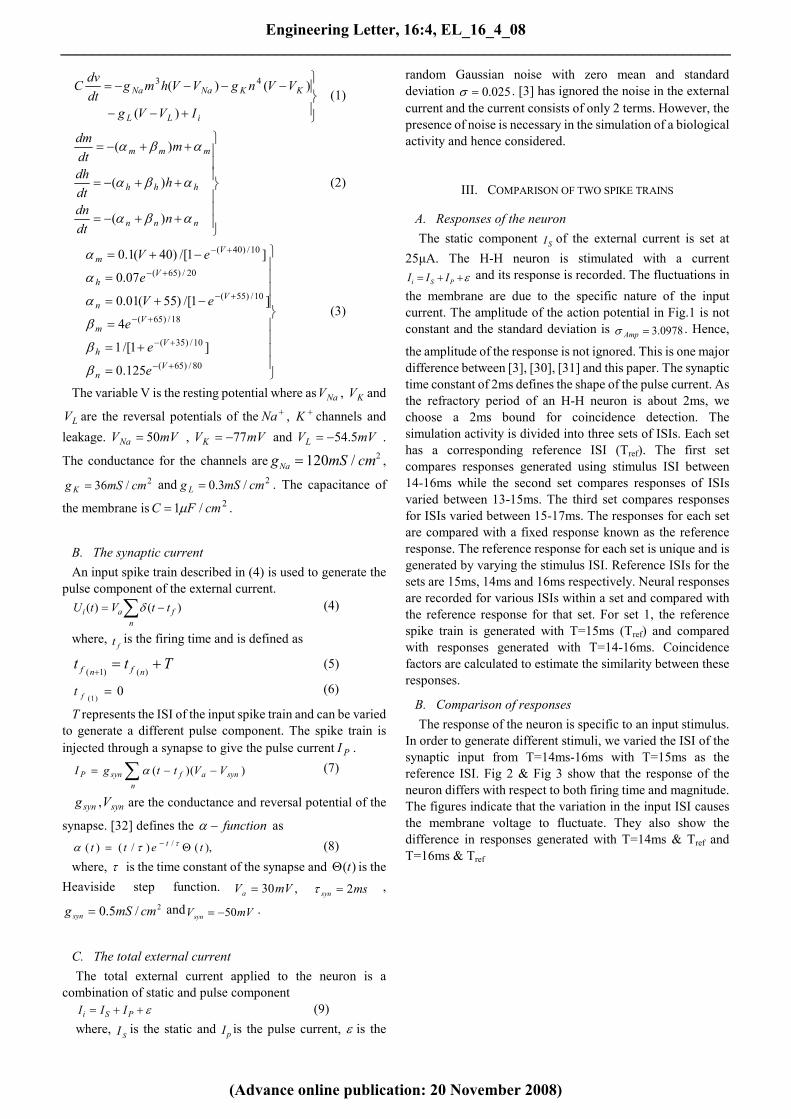
C. The total external current

The total external current applied to the neuron is a

combination of static and pulse component

ε++= PSi III (9)

where, SI is the static and pI is the pulse current, ε is the

random Gaussian noise with zero mean and standard

deviation 025.0=σ . [3] has ignored the noise in the external

current and the current consists of only 2 terms. However, the

presence of noise is necessary in the simulation of a biological

activity and hence considered.

III. COMPARISON OF TWO SPIKE TRAINS

A. Responses of the neuron

The static component SI of the external current is set at

25µA. The H-H neuron is stimulated with a current

ε++= PSi III and its response is recorded. The fluctuations in

the membrane are due to the specific nature of the input

current. The amplitude of the action potential in Fig.1 is not

constant and the standard deviation is 0978.3=Ampσ . Hence,

the amplitude of the response is not ignored. This is one major

difference between [3], [30], [31] and this paper. The synaptic

time constant of 2ms defines the shape of the pulse current. As

the refractory period of an H-H neuron is about 2ms, we

choose a 2ms bound for coincidence detection. The

simulation activity is divided into three sets of ISIs. Each set

has a corresponding reference ISI (Tref). The first set

compares responses generated using stimulus ISI between

14-16ms while the second set compares responses of ISIs

varied between 13-15ms. The third set compares responses

for ISIs varied between 15-17ms. The responses for each set

are compared with a fixed response known as the reference

response. The reference response for each set is unique and is

generated by varying the stimulus ISI. Reference ISIs for the

sets are 15ms, 14ms and 16ms respectively. Neural responses

are recorded for various ISIs within a set and compared with

the reference response for that set. For set 1, the reference

spike train is generated with T=15ms (Tref) and compared

with responses generated with T=14-16ms. Coincidence

factors are calculated to estimate the similarity between these

responses.

B. Comparison of responses

The response of the neuron is specific to an input stimulus.

In order to generate different stimuli, we varied the ISI of the

synaptic input from T=14ms-16ms with T=15ms as the

reference ISI. Fig 2 & Fig 3 show that the response of the

neuron differs with respect to both firing time and magnitude.

The figures indicate that the variation in the input ISI causes

the membrane voltage to fluctuate. They also show the

difference in responses generated with T=14ms & Tref and

T=16ms & Tref



Fig 1: Response of the H-H neuron to iI with T=15ms causing fluctuations

in membrane voltage. (a) The synaptic spike train input that induces a pulse

current. (b)The pulse current generated. (c) The total external current

ε++ PS II applied to the neuron. Note that there is a static offset (d) The

neuronal response to the current.

50 100 150 200 250 30010

15

20

25

(a) Time

Sp

ike

Po

ints

50 100 150 200 250 300-100

-50

0

50

(b) Time

Vo

lta

ge

T=15ms

T=16ms

Fig 2: Comparison of responses. (a) The corresponding magnitude of spikes

for the responses at T=16ms and T=15ms. (b) The two spike trains not only

differ in firing times but also in magnitudes.

50 100 150 200 250 30010

15

20

25

(a) Time

Sp

ike

Po

ints

50 100 150 200 250 300-100

-50

0

50

(b) Time

Vo

lta

ge

T=15ms

T=14ms

Fig 3: Comparison of responses. (a) The corresponding magnitude of spikes

for the responses at T=14ms and T=15ms. (b) The two spike trains not only

differ in firing times but also in magnitudes.

C. Coincidence- factor

The coincidence-factor, as described by [18], [20] is 1 only

if the two spike trains are exactly the same and 0 if they are

very dissimilar. Coincidence for an individual spike is

established if its firing time is within 2ms of the firing time of

the corresponding spike in the reference spike train (in this

case T=15ms). The mathematical equations are discussed

very briefly here as they are discussed in detail in [20]. The

coincidence-factor is given by

NNN

NN coinccoinc 1

)(2/1 21 +

⟩⟨−=Γ (10)

where, 1N is the number of spikes in the reference train,

2N is the number of spikes in the train to be compared,

coincN is the number of coincidences with a precision

ms2=δ between the spike trains. 12 NN coinc νδ=⟩⟨ is the

expected number of coincidences generated by a

homogeneous Poisson process with the same rate as the spike

train to be compared. νδ21−=N is the normalising factor.

For set 1, 1N is the number of spikes in the reference spike

train (Tref=15ms) and 2N is the number of spikes in the train

to be compared (T=14-16ms). Fig.4 shows that the

coincidence-factors for responses generated using T=

14-16ms do not follow a fixed pattern. The coincidence-factor

( Γ ) is expectedly 1 when spike train generated with T=15ms

is compared with the reference spike train Tref (T=15ms).

However, the coincidence factor for spike trains generated at

T=16ms and Tref is 1. This indicates that the two highly

varying currents have an exactly similar response or

conversely as the responses are same; the two input stimuli are

similar, which is an incorrect inference. The coincidence

factor for the spike trains generated at T=14ms and Tref is

0.1207 indicating very low similarity. From a mathematical

and signal transmission standpoint, the coincidence-factor

should decrease as the input stimulus increasingly varies from

Tref. However, this can only be observed between

T=14.65ms-15.25ms (30% of the 2ms time window). The

coincidence-factor Γ increases from T=14ms-14.5ms but

then drops till T=14.65ms. Γ steadily increases to 1 when

T=15ms and drops for 0.25ms. There is an upward rise from

T=15.25ms-15.5ms, a sharp drop from T=15.5ms-15.75ms

followed by a steep increase to 1=Γ at T=16ms. Traversing

from the reference the expected trajectory of the

coincidence-factor breaks at T=14.65ms and T=15.25ms.

These are therefore taken as limits for faithful behaviour of

the coincidence-factor approach. However, for set 2 reference

spike train is chosen as Tref=14ms, limits of faithful behaviour

change (Fig. 5). The coincidence factor steadily rises to unity,

stays there for 0.5ms and drops gradually. Ideally, the

coincidence-factor should be not 1 for T=13.5, 13.65 and

13.75. While in set 3, Fig. 6, reference spike train chosen is at

Tref=16ms. The limits of faithful behaviour change with a

change in the stimulus. There is a sharp rise in the coincidence

factor from 15.75ms to 16ms where it reaches unity. From

16ms to 17ms the coincidence-factor executes a perfect curve

as expected. From figures 4, 5 and 6 it is conclusive that the

lower-bound of faithful behaviour increases with the increase

in the input reference ISI. The difference between the

reference ISI (Tref) and the lower-bound limit decreases with

the increase in the reference ISI. It is also important to note



that within each set of simulation, there are some false

coincidences. The term false coincidence is used to identify

comparisons whose coincidence factor is 1 - when it should

not be. In Fig.4, there is a false coincidence when ISI = 16ms

is compared with Tref = 15ms. In Fig. 5, false coincidences can

be seen when ISI varied between 13.5-13.75ms is compared

with Tref = 14ms while in Fig. 6, false coincidences can be

observed for ISI varied between 15-15.15ms and compared

with Tref = 16ms.

14 14.2 14.4 14.6 14.8 15 15.2 15.4 15.6 15.8 160

0.2

0.4

0.6

0.8

1

1.2

Inter-Spike-Interval

Co

inc

ide

nc

e f

ac

to

r

Expected

decrease in the

coincidence

factor with

increase in ISI

from the

reference spike

train

Inconsistent result Inconsistent result

Concidence factor =1

Reference, T=15m s

Fig 4: Coincidence-factor versus ISI. The coincidence-factor decreases

expectedly between T=15ms-14.65ms and T=15ms-15.25ms. At other times

the result is inconsistent and does not have a fixed pattern.

13 13.2 13.4 13. 6 13.8 14 14.2 14. 4 14.6 14.8 15

0

0.2

0.4

0.6

0.8

1


Co

inc

ide

nc

e F

ac

tor

Faithful behaviour

Reference

T=14ms

Fig 5: Coincidence-factor versus ISI. The coincidence-factor has a faithful

behaviour between T=13.15ms - 14.65ms.

15 15.2 15.4 15.6 15.8 16 16.2 16.4 16.6 16.8 17

0

0.2

0.4

0.6

0.8

1


Co

inc

ide

nc

e F

ac

tor

Faithful behaviour

Reference

T=16ms

Fig 6: Coincidence-factor versus ISI. The coincidence-factor has a faithful

behaviour between T=15.75ms - 17ms. It executes a perfect curve after

16ms.

D. Two-dimensional analysis

The coincidence-factors over the 2ms time window show

an inconsistent trend. A 1-dimensional approach of the

coincidence-factor determination is thought to be the cause of

this inconsistency. The coincidence-factor is highly accurate

for spike trains with a constant amplitude response however;

the coincidence-factor does not give a proper estimate of

similarity between two spike trains with varying amplitudes.

As a result, two visually distinct spike trains would still

generate a high coincidence-factor (Fig. 2 & Fig. 3). A

2-dimensional analysis of spike trains with fluctuating

magnitudes can resolve this inconsistency. To support this, a

simple binary clustering algorithm is used. It shows that the

clustering solution for each response is unique and therefore

helps to eliminate any ambiguity.

E. Binary clustering

The peak of each spike in the spike train is considered as an

object. The object (Obj) is defined as point with its firing time

and amplitude. The number of objects for each spike train is

equal to the number of spikes.

],[ AmplitudeFiringtimeObj = (11)

We calculate the Euclidean distances between objects in

each spike train using '2

))(( srsrrs NNNNd −−= (12)

where rN , SN are the objects in the spike train. Once the

distance between each pair of objects is determined, the

objects are clustered based on the nearest neighbour approach

using

∈∈

−=

),...,1(),,...,1(

))(min(),(

sr

sjri

njni

NNdistsrd (13)

where sr nn , is the total number of objects in the respective

clusters. The binary clusters are plotted to form a hierarchical

tree whose vertical links indicate the distance between two

objects linked to form a cluster. A number is assigned to each

cluster as soon as it is formed. Numbering starts from (m+1),

where m=initial number of objects, till no more clusters can

be formed.

We investigated the case described in section 3.3 for the

response generated at Tref=15ms and T=16ms (false

coincidence). The coincidence-factor for these two responses

is 1 (Fig. 4) and indicates an exact match between the two.

The clustering solution shows that these two responses are

actually different from each other by a margin not captured by

the coincidence-factor (Fig. 7 & Fig. 8). The clustered objects

are shown on the X-axis and the distance between them is

shown on the Y-axis. A comparison of the clustering solutions

shows that the shape, form, height as well as linkages are

different for the two spike trains. This mean that the spikes

clustered together in each train are different. In fig. 7 objects

12 and 13 are clustered together at a height of 11.5 while in

fig.8, objects 11 and 12 are clustered at a height of 13.5 –

shown in green circles. Also, objects 4 and 5 are clustered in

fig. 7 while objects 3 and 4 are clustered in fig. 8 – shown in

red circles. It indicates that the two spike trains are inherently

different by a margin not captured by the coincidence factor.

The results hence prove that the two spike trains are not an

exact match. We therefore believe that though determining



coincidence-factor is important, a two-dimensional analysis is

necessary for a response with a fluctuating membrane voltage.

Fig 7: Clustering solution for T=15ms indicating objects being clustered

Fig 8: Clustering solution for T=16ms indicating objects being clustered

IV. CONCLUSIONS

The response of a neuron to a time-varying stimulus has

been studied before and the complexity of the H-H model has

led neuroscientists to develop simpler models that reconstruct

the firing pattern of a biological neuron [17]-[28]. Recently,

comparisons have been made between responses and

similarity measures proposed [18], [20], [23]-[26], [30], [31].

However, the responses considered have a constant

magnitude thereby making their analysis one-dimensional.

A synaptic stimulus known to induce fluctuations in the

membrane voltage is used to stimulate an H-H neuron [3] to

verify if firing time alone is enough to differentiate between

these responses. The time constant of the pulse component of

the external current is 2ms and due to refractoriness of the

neuron, coincidence-bound is also chosen as 2ms. The

coincidence-factors are calculated for time

windows mst 16141 −= , mst 15132 −= and

msmst 17153 −= with reference spike trains at T=15ms,

14ms and 16ms respectively. In all three sets of results, there

is no consistent trend exhibited by the coincidence-factor.

Also, the limits of faithful behaviour change and the

percentage of acceptable results varies. The percentage of

faithful behaviour for the three time windows is 30, 75 and

62.5 respectively. The main findings through these sets of

results are: (a) the limits of faithful behaviour change with a

change in the reference ISI. (b) the lower-bound limit of

faithful behaviour increases with the increase of the reference

ISI. (c) the difference between the reference ISI and the

lower-bound limit of faithful behaviour decreases with the

increase in the reference ISI. This is shown to be due to the

one-dimensional similarity measure undertaken. In order to

differentiate between these responses accurately, a

two-dimensional analysis is required as the magnitudes of the

action potentials are vital. A simple clustering algorithm is

seen to easily differentiate between two visually-distinct

responses as opposed to the coincidence-factor approach.

Thus a two-dimensional analysis to differentiate between such

responses is necessary and we are currently working towards

a more robust differentiation strategy which also quantifies

the difference between responses.

The aim of using clustering technique is to exemplify the

requirement of a two-dimensional analysis. We take this as a

supporting claim for our future work.

REFERENCES

[1] Lundström I (1974). Mechanical Wave Propagation on Nerve

Axons. Journal of Theoretical Biology, 45, 487-499.

[2] Abbott LF, Kepler TB (1990). Model Neurons: From Hodgkin

Huxley to Hopfield. Statistical Mechanics of Neural Networks,

Edited by Garrido L, 5-18.

[3] Hasegawa H (2000). Responses of a Hodgkin-Huxley neuron to

various types of spike-train inputs. Physical Review E, Vol. 61,

No. 1.

[4] Kepecs A, Lisman J (2003). Information encoding and

computation with spikes and bursts. Network: Comput. Neural

Syst. 14, 103-118.

[5] Fourcaud-Trocmé N, Hansel D, van Vreeswijk C, Brunel N

(2003). How Spike Generation Mechanisms Determine the

Neuronal Response to Fluctuating Inputs. The Journal of

Neuroscience, 23(37): 11628-11640.

[6] Bokil HS, Pesaran B, Andersen RA, Mitra PP (2006). A Method

for Detection and Classification of Events in Neural Activity.

IEEE Transactions on Biomedical Engineering, Vol. 53, No. 8.

[7] Davies RM, Gerstein GL, Baker SN (2006). Measurement of

Time-Dependent Changes in the Irregularity of Neural Spiking.

Journal of Neurophysiology, 96:906-918.

[8] Diba K, Koch C, Segev I (2006). Spike Propagation in dendrites

with stochastic ion channels. Journal of Computational

Neuroscience 20: 77-84.

[9] Dimitrov AG, Gedeon T (2006). Effects of stimulus

transformations on estimates of sensory neuron selectivity.

Journal of Computational Neuroscience 20: 265-283.

[10] Rinzel J (1985). Excitation dynamics: insights from simplified

membrane models. Theoretical Trends in Neuroscience Federal

Proceedings, Vol. 44, No. 15, 2944-2946.

[11] Gabbiani F, Metzner W (1999). Encoding and Processing of

Sensory Information in Neuronal Spike Trains. The Journal of

Biology, 202, 1267-1279.

[12] Panzeri S, Schultz SR, Treves A, Rolls ET (1999). Correlations

and the encoding of information in the nervous system. Proc. R.

Soc. Lond. B 266, 1001-1012.



[13] Agüera y Arcas B, Fairhall AL (2003). What causes a Neuron to

Spike? Neural Computation 15, 1789-1807, (2003).

[14] Agüera y Arcas B, Fairhall AL, Bialek W (2003). Computation in

a Single Neuron: Hodgkin and Huxley Revisited. Neural

Computation 15, 1715-1749.

[15] Izhikevich EM (2006). Polychronization: Computation with

Spikes. Neural Computation 18, 245-282.

[16] Li X, Ascoli GA (2006). Computational simulation of the

input-output relationship in hippocampal pyramidal cells.

Journal of Computational. Neuroscience, 21:191-209.

[17] Kepler TB, Abbott LF, Marder E (1992). Reduction of

conductance-based neuron models. Biological Cybernetics, 66,

381-387.

[18] Joeken S, Schwegler H (1995). Predicting spike train responses

of neuron models; in M.Verleysen (ed.), Proceedings of the 3rd

European Symposium on Artificial Neural Networks, pp. 93-98.

[19] Wang XJ, Buzsáki G (1996). Gamma Oscillation by Synaptic

Inhibition in a Hippocampal Interneuronal Network Model. The

Journal of Neuroscience, 16(20): 6402-6413.

[20] Kistler WM, Gerstner W, Leo van Hemmen J (1997). Reduction

of the Hodgkin-Huxley Equations to a Single-Variable Threshold

Model. Neural Computation 9: 1015-1045.

[21] Izhikevich EM (2003). Simple Model of Spiking Neurons. IEEE

Transactions on Neural Networks, Vol. 14 No. 6.

[22] Shriki O, Hansel D, Sompolinsky H (2003). Rate Models for

Conductance-Based Cortical Neuronal Networks. Neural

Computation 15, 1809-1841.

[23] Jolivet R, Gerstner W (2004). Predicting spike times of a detailed

conductance-based neuron model driven by stochastic spike

arrival. Journal of Physiology – Paris 98, 442-451.

[24] Jolivet R, Lewis TJ, Gerstner W (2004). Generalized

Integrate-and-Fire Models of Neuronal Activity Approximate

Spike Trains of a Detailed Model to a High Degree of Accuracy.

Journal of Neurophysiology 92: 959-976.

[25] Jolivet R, Rauch A, Lüscher H-R, Gerstner W (2006).

Integrate-and-Fire models with adaptation are good enough:

predicting spike times under random current injection. Advances

in Neural Information Processing Systems 18: 595-602.

[26] Jolivet R, Rauch A, Lüscher H-R, Gerstner W (2006). Predicting

spike timing of neocortical pyramidal neurons by simple

threshold models. Journal of Computational Neuroscience 21:

35-49.

[27] Clopath C, Jolivet R, Rauch A, Lüscher H-R, Gerstner W (2007).

Predicting neuronal activity with simple models of the threshold

type: Adaptive Exponential Integrate-and-Fire model with two

compartments. Neurocomputing 70: 1668-1673.

[28] Djabella K, Sorine M (2007). Reduction of a Cardiac Pacemaker

Cell Model Using Singular Perturbation Theory. Proceedings of

the European Control Conference 2007, Kos, Greece,

3740-3746.

[29] Hodgkin A, Huxley A (1952). A quantitative description of

membrane current and its application to conduction and

excitation in nerve. J. Physiol. 117:500–544.

[30] Maršálek, P (2000). Coincidence detection in the

Hodgkin–Huxley equations. Biosystems, Vol. 58, Issues 1-3.

[31] Victor JD, Purpura KP (1997). Metric-space analysis of spike

trains: theory, algorithms and application. Network: Comput.

Neural Syst. 8 127-164.

[32] Park MH, Kim S (1996). Analysis of Phase Models for two

Coupled Hodgkin-Huxley Neurons. Journal of the Korean

Physical Society, Vol. 29, No. 1, pp. 9-16.



Documents

Spiking Neurons and Synaptic Stimuli: Determining the ... · Abstract— Similarity between two spike trains is generally ... University of Hull, Hull, East-Yorkshire, HU6 7RX, UK