Embed Size (px)
Citation preview
Spherical Shallow Water Turbulence:Cyclone-Anticyclone Asymmetry,
Potential Vorticity Homogenisation and Jet Formation
Jemma ShiptonDepartment of Atmospheric, Oceanic and Planetary Physics,
University of Oxford
David DritschelDepartment of Applied Mathematics,
University of St Andrews
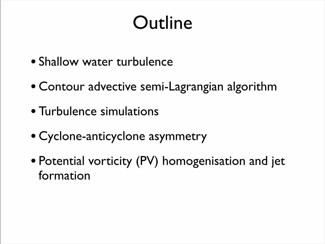
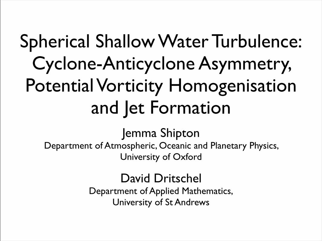
Outline
• Shallow water turbulence
• Contour advective semi-Lagrangian algorithm
• Turbulence simulations
• Cyclone-anticyclone asymmetry
• Potential vorticity (PV) homogenisation and jet formation
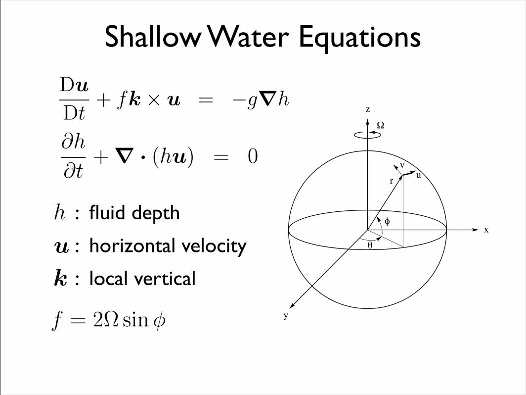
Shallow Water Equations
Du
Dt! fv = !g
!h
!x, (2.8)
Dv
Dt+ fu = !g
!h
!y, (2.9)
where f = 2! sin" is the Coriolis parameter. Equations 2.8-2.9 shows that if the
horizontal velocities u and v are initially independent of depth they will remain so
as the Coriolis and pressure gradient forces are also independent of depth. This
enables us to integrate equation 2.1 from z = 0 (the lower boundary) to z = h
(the depth of the fluid) to obtain
h
!
!u
!x+
!v
!y
"
+ w(h) ! w(0) = 0. (2.10)
At z = 0 there can be no flow normal to the boundary so w(0) = 0 while at
the free surface w(h) = Dh/Dt. So, in vector form, equations 2.8 - 2.10 can be
written
Du
Dt+ fk " u = !g!h (2.11)
!h
!t+ ! · (hu) = 0 (2.12)
where u is the horizontal velocity and only the two components perpendicular to
k, the local vertical, of equation 2.11 are considered.
The shallow water equations 2.11-2.12 are commonly expressed in terms of
the vertical component of the relative vorticity # = vx ! uy and the divergence
$ = ux + vy:
D#
Dt+ (# + f)$ ! %v = 0, (2.13)
D$
Dt+ $2 ! 2J(u, v) ! f# + %u = !g#2h, (2.14)
26
Du
Dt! fv = !g
!h
!x, (2.8)
Dv
Dt+ fu = !g
!h
!y, (2.9)
where f = 2! sin" is the Coriolis parameter. Equations 2.8-2.9 shows that if the
horizontal velocities u and v are initially independent of depth they will remain so
as the Coriolis and pressure gradient forces are also independent of depth. This
enables us to integrate equation 2.1 from z = 0 (the lower boundary) to z = h
(the depth of the fluid) to obtain
h
!
!u
!x+
!v
!y
"
+ w(h) ! w(0) = 0. (2.10)
At z = 0 there can be no flow normal to the boundary so w(0) = 0 while at
the free surface w(h) = Dh/Dt. So, in vector form, equations 2.8 - 2.10 can be
written
Du
Dt+ fk " u = !g!h (2.11)
!h
!t+ ! · (hu) = 0 (2.12)
where u is the horizontal velocity and only the two components perpendicular to
k, the local vertical, of equation 2.11 are considered.
The shallow water equations 2.11-2.12 are commonly expressed in terms of
the vertical component of the relative vorticity # = vx ! uy and the divergence
$ = ux + vy:
D#
Dt+ (# + f)$ ! %v = 0, (2.13)
D$
Dt+ $2 ! 2J(u, v) ! f# + %u = !g#2h, (2.14)
26
If we now consider the vertical component for a fluid at rest we obtain
1
ρ
∂p
∂z= !g.
This equation states that the vertical pressure gradient is balanced by gravity.This is known as hydrostatic balance.
In taking the hydrostatic approximation we assume that the vertical accelerationis negligible compared to the vertical pressure gradient.
Integrate with the boundary condition that p(x, y, h) = p0 gives
p(z) = ρg(h! z) + p0.
Eliminate p from the horizontal momentum equations:
Du
Dt! fv = !g
∂h
∂x,
Dv
Dt+ fu = !g
∂h
∂y,
where f = 2! sin φ is the Coriolis parameter.
2
Integrate ! ·u from z = 0 (the lower boundary) to z = h (the depth of the fluid)to obtain
h
!!u
!x+
!v
!y
"+ w(h)− w(0) = 0.
At z = 0 there can be no flow normal to the boundary so w(0) = 0 while at thefree surface w(h) = Dh/Dt. So, in vector form we have:
Du
Dt+ fk × u = −g!h (1)
!h
!t+ ! · (hu) = 0 (2)
where u is the horizontal velocity and only thetwo components perpendicular to k, the localvertical, of equation ?? are considered.
3
Integrate ! ·u from z = 0 (the lower boundary) to z = h (the depth of the fluid)to obtain
h
!!u
!x+
!v
!y
"+ w(h)! w(0) = 0.
At z = 0 there can be no flow normal to the boundary so w(0) = 0 while at thefree surface w(h) = Dh/Dt. So, in vector form we have:
Du
Dt+ fk " u = !g!h (1)
!h
!t+ ! · (hu) = 0 (2)
where u is the horizontal velocity and only thetwo components perpendicular to k, the localvertical, of equation ?? are considered.
3
: fluid depth
: horizontal velocity
: local vertical
uv
!
"
#
r
x
y
z
Shallow Water Equations
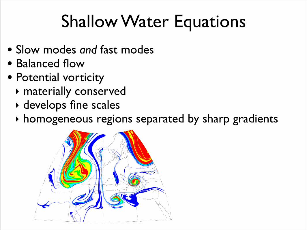
• Slow modes and fast modes• Balanced flow• Potential vorticity‣ materially conserved‣ develops fine scales‣ homogeneous regions separated by sharp gradients
Shallow Water Equations
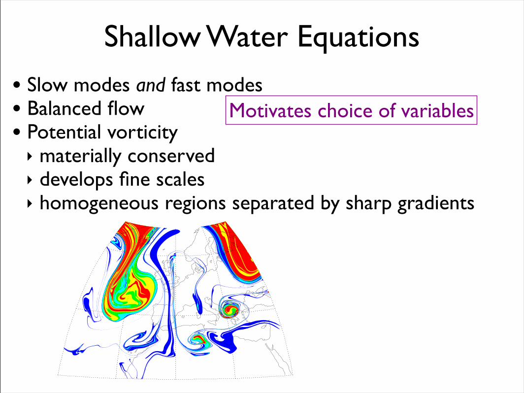
• Slow modes and fast modes• Balanced flow• Potential vorticity‣ materially conserved‣ develops fine scales‣ homogeneous regions separated by sharp gradients
Motivates choice of variables
Shallow Water Equations
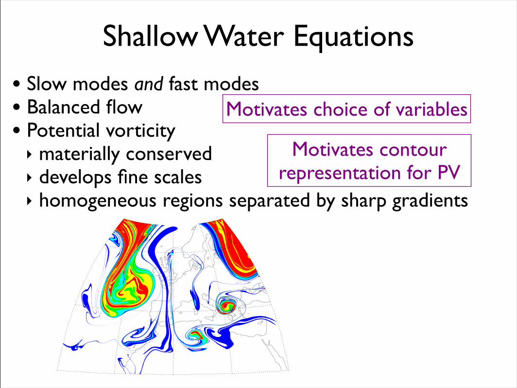
• Slow modes and fast modes• Balanced flow• Potential vorticity‣ materially conserved‣ develops fine scales‣ homogeneous regions separated by sharp gradients
Motivates choice of variables
Motivates contour representation for PV
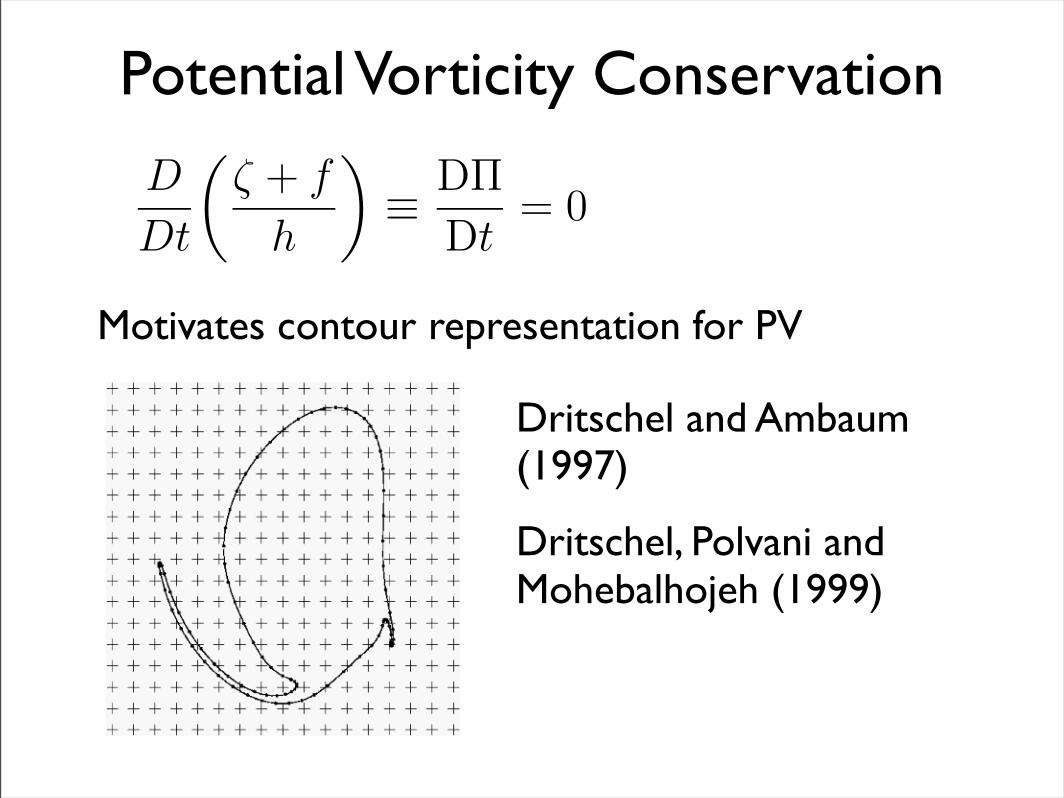
Potential Vorticity Conservation
where ! = "f/"y. Rewriting equation 2.12 in the form
Dh
Dt+ h# = 0 (2.15)
enables us to eliminate # from equation 2.13 to give
D
Dt
!
$ + f
h
"
!D!
Dt= 0, (2.16)
where
! !$ + f
h(2.17)
is the potential vorticity (PV). Equation 2.16 states that the PV is conserved
following a fluid parcel. Although equation 2.16 has been derived using several
assumptions, in particular the absence of forcing, it is still approximately true in
atmospheric and oceanic flows provided the timescale of the flow under consider-
ation short enough (< 4 days McIntyre [2002b]).
2.2 Linearised equations
In chapter 1 we stated that the PV controls the dominant large scale ‘balanced’
motion. Here we show this using the linear equations.
Linearising equations 2.11-2.12 about a state of rest (u = 0, h = H) and
taking f to be constant gives
27
Motivates contour representation for PV
Dritschel and Ambaum (1997)
Dritschel, Polvani and Mohebalhojeh (1999)
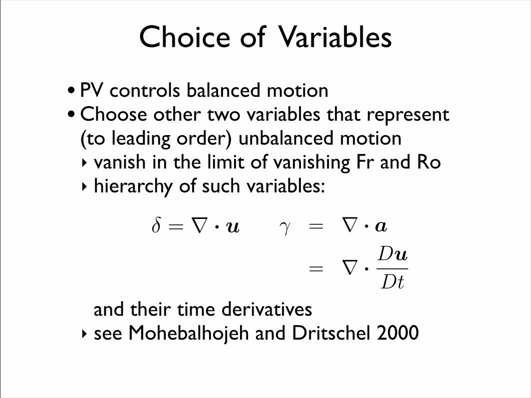
Choice of Variables
• PV controls balanced motion• Choose other two variables that represent
(to leading order) unbalanced motion‣ vanish in the limit of vanishing Fr and Ro‣ hierarchy of such variables:
and their time derivatives‣ see Mohebalhojeh and Dritschel 2000
of the variables (layer depth h and horizontal velocity u) that are directly useful
for visualising the fluid flow. However, this form of the equations hides some
underlying mathematical properties such as the Lagrangian conservation of PV
(equation 2.16). It has been shown [Dritschel and Viudez, 2003, Mohebalhojeh
and Dritschel, 2000b] to be beneficial to rewrite the equations in terms of dif-
ferent variables. Since the PV field is central to the balanced dynamics and has
the property that it is materially conserved, ! is a natural choice for one of the
prognostic variables. This is unconventional but not unprecedented. Thuburn
[1996], Bates et al. [1995] and Temperton and Staniforth [1987] for example, each
employ models that use PV as a prognostic variable. Here we use the contour
advection method developed by Dritschel and Ambaum [1997] and Dritschel et al.
[1999]. This method is outlined in the following section.
Given equation 2.16 as one of our prognostic equations, we now have to choose
the other two variables. A common variable choice is (!, ", h) so an obvious choice
would be to replace the vorticity ! with potential vorticity ! and keep the other
two variables. However, small errors in calculating the nonlinear terms in the
prognostic equation for h can result in erroneous gravity waves in the divergence
field [Dritschel and Mohebalhojeh, 2000]. Numerous studies (for example Mo-
hebalhojeh and Dritschel [2000b], Dritschel and Viudez [2003] and Smith and
Dritschel [2006]) have shown that it is advantageous to avoid evolving h and in-
stead use prognostic equations for variables that vanish in the limit of vanishing
Rossby and Froude numbers. Equations of this form then have the property that
geostrophic balance is recovered, as expected, when Fr ! Ro " 1. Mohebalhojeh
and Dritschel [2000a] derive hierarchies of variables for which this is true. Their
hierarchies are based on the variables " and # (and their time derivatives), where
" = # · u, (2.72)
is the divergence (as introduced in section 2.1) and
38
! = ! · a (2.73)
= ! ·Du
Dt(2.74)
= f" " #u " c2!2h, (2.75)
is the divergence of the acceleration a. Note that for for constant background
rotation (# = 0), !/f is the ageostrophic vorticity. It has been shown that
in this case, i.e. on an f-plane, that $ and ! themselves are the best choice of
variables over a wide range of Fr and Ro [Mohebalhojeh and Dritschel, 2000b].
It is not obvious that these variables should work so well on the sphere due to
the breakdown of geostrophic balance at the equator. However, we shall see in
chapter 4 that they are remarkably e!ective.
The prognostic equations for $ and ! in spherical coordinates [Smith and
Dritschel, 2006]1 are
$t = ! " |u|2 " 2[u!(u! + ") + v!(v! " $)] " ! · ($u), (2.76)
!t = c2!2{! · [(1 + h)u]} + 2"B" " ! · (Zu), (2.77)
where c2 # gH (mean-square gravity wave speed), B # c2h " 12 |u|
2 (Bernoulli
pressure), and Z = f(" + f). We now have three prognostic equations for the
variables (#,$,!). However, we still need h, u and v to solve these equations.
Writing u as the sum of a streamfunction and divergence potential we have
u = k $ !% + !&, (2.78)
where1some of the work here was completed before publication in Smith and Dritschel [2006]
39
Turbulence Simulations
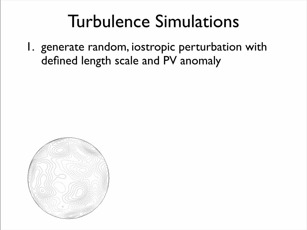
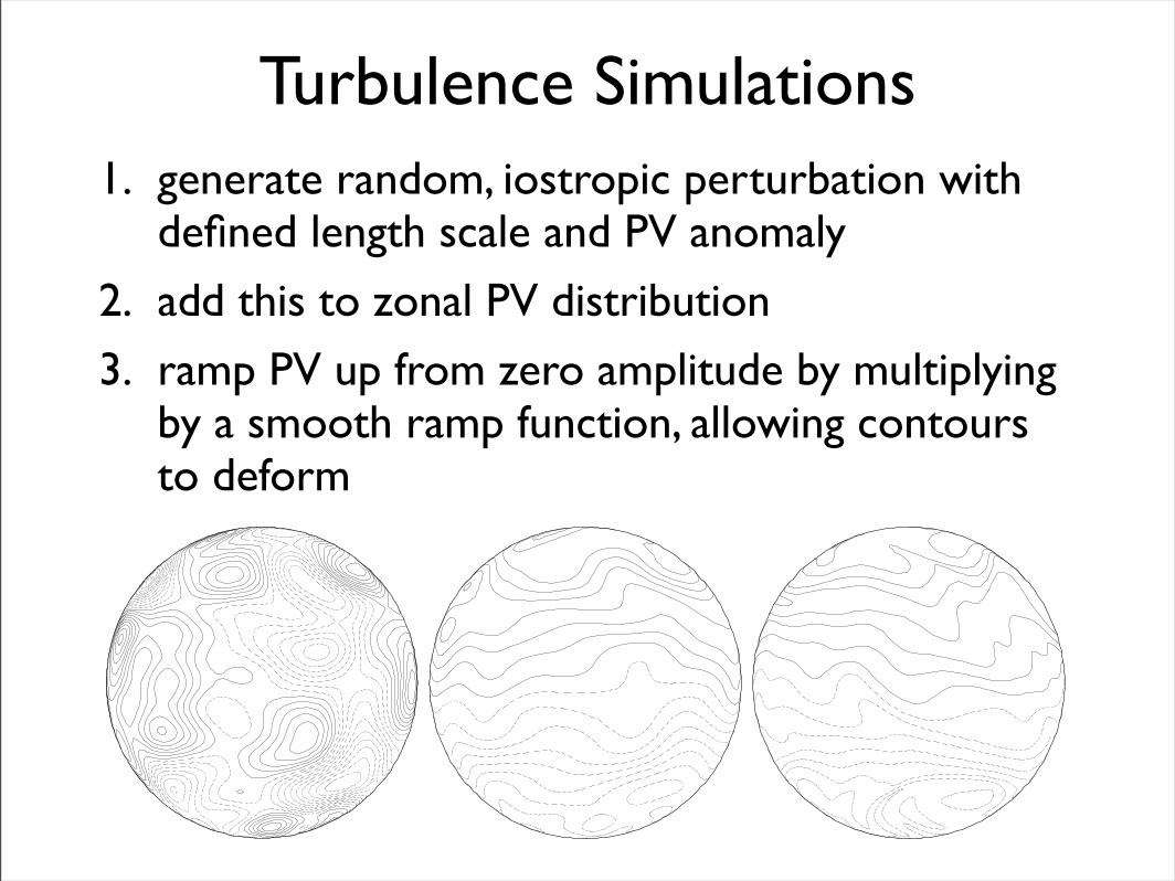
Turbulence Simulations1. generate random, iostropic perturbation with
defined length scale and PV anomaly
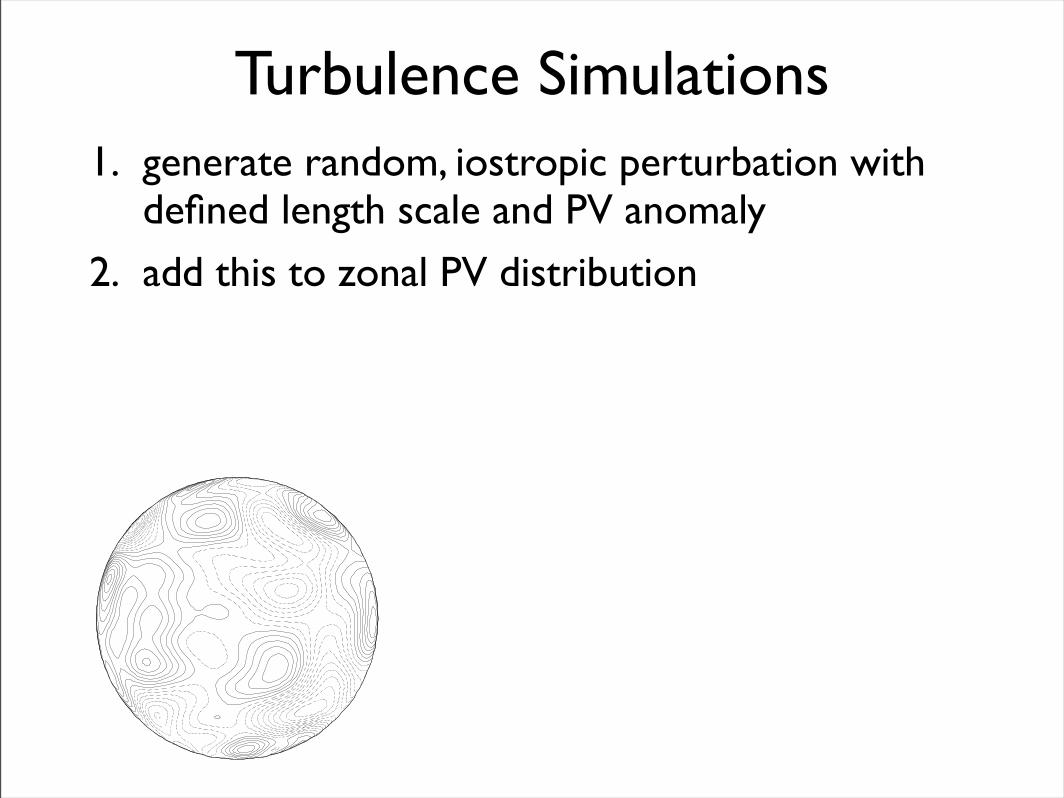
Turbulence Simulations1. generate random, iostropic perturbation with
defined length scale and PV anomaly
Turbulence Simulations1. generate random, iostropic perturbation with
defined length scale and PV anomaly
2. add this to zonal PV distribution
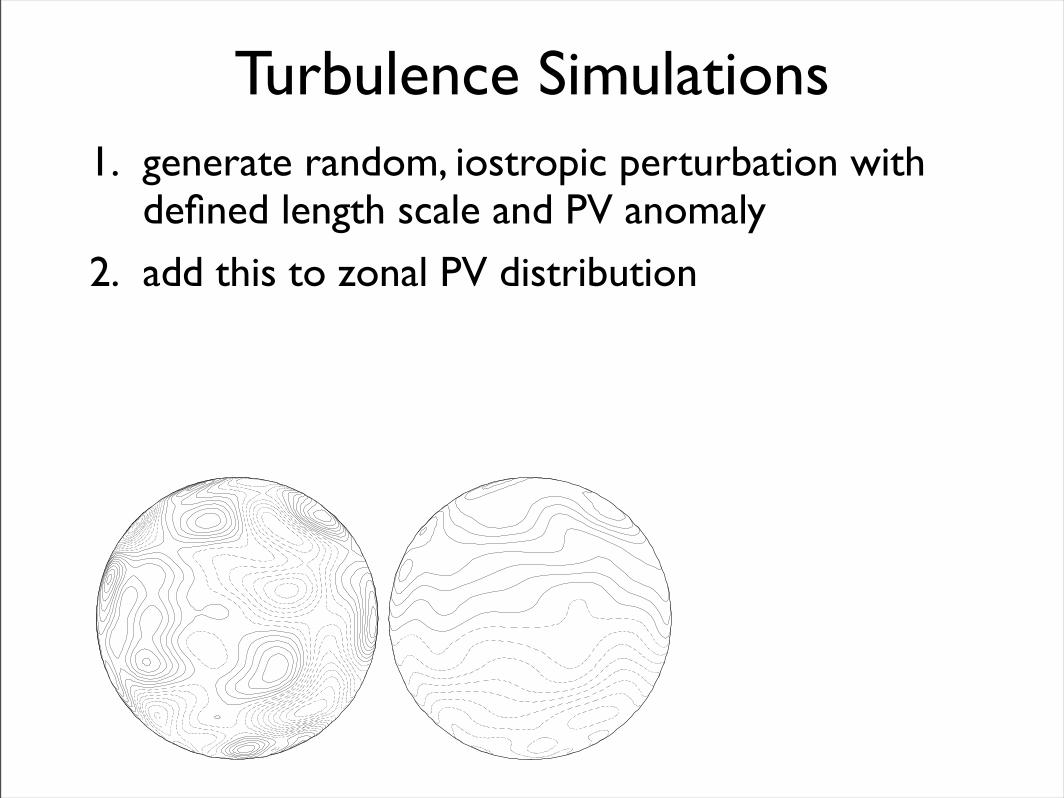
Turbulence Simulations1. generate random, iostropic perturbation with
defined length scale and PV anomaly
2. add this to zonal PV distribution
Turbulence Simulations1. generate random, iostropic perturbation with
defined length scale and PV anomaly
2. add this to zonal PV distribution
3. ramp PV up from zero amplitude by multiplying by a smooth ramp function, allowing contours to deform
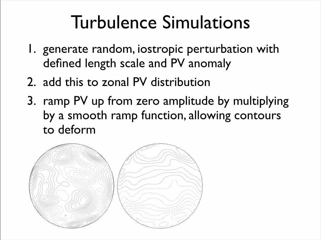
Turbulence Simulations1. generate random, iostropic perturbation with
defined length scale and PV anomaly
2. add this to zonal PV distribution
3. ramp PV up from zero amplitude by multiplying by a smooth ramp function, allowing contours to deform
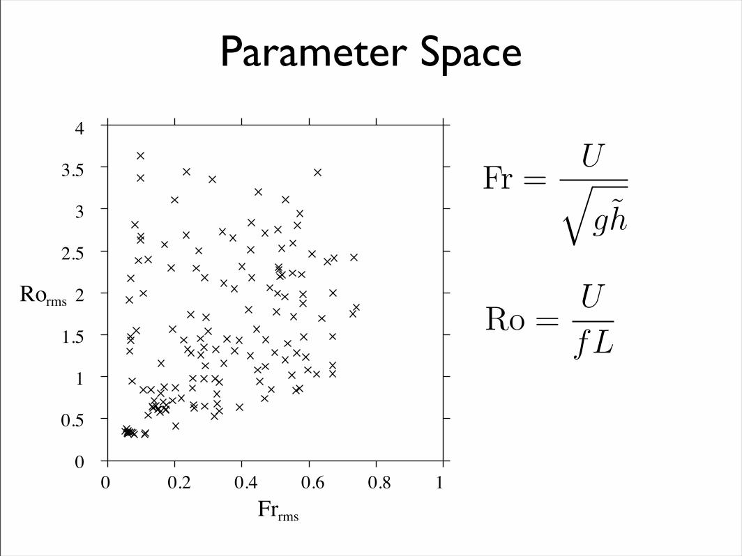
Parameter Space
Fr =U!gh
Ro =U
fL
h!
14
Fr =U!gh
Ro =U
fL
h!
14
0
0.5
1
1.5
2
2.5
3
3.5
4
0 0.2 0.4 0.6 0.8 1Frrms
Rorms
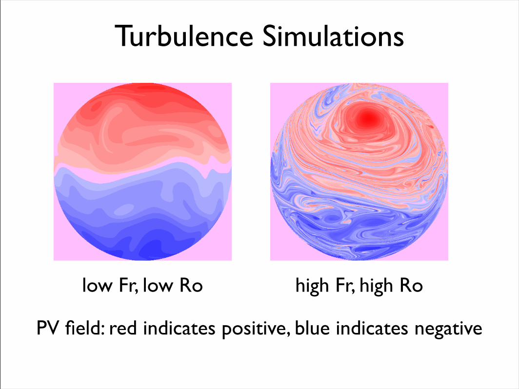
low Fr, low Ro high Fr, high Ro
PV field: red indicates positive, blue indicates negative
Turbulence Simulations
Cyclone-Anticyclone AsymmetryCase 1
h~-0.025 0.025
0
0.07
Case 2
h~-0.02 0.02
0
0.07
Case 3
h~-0.6 0.6
0
0.05
Case 4
h~-0.3 0.3
0
0.04
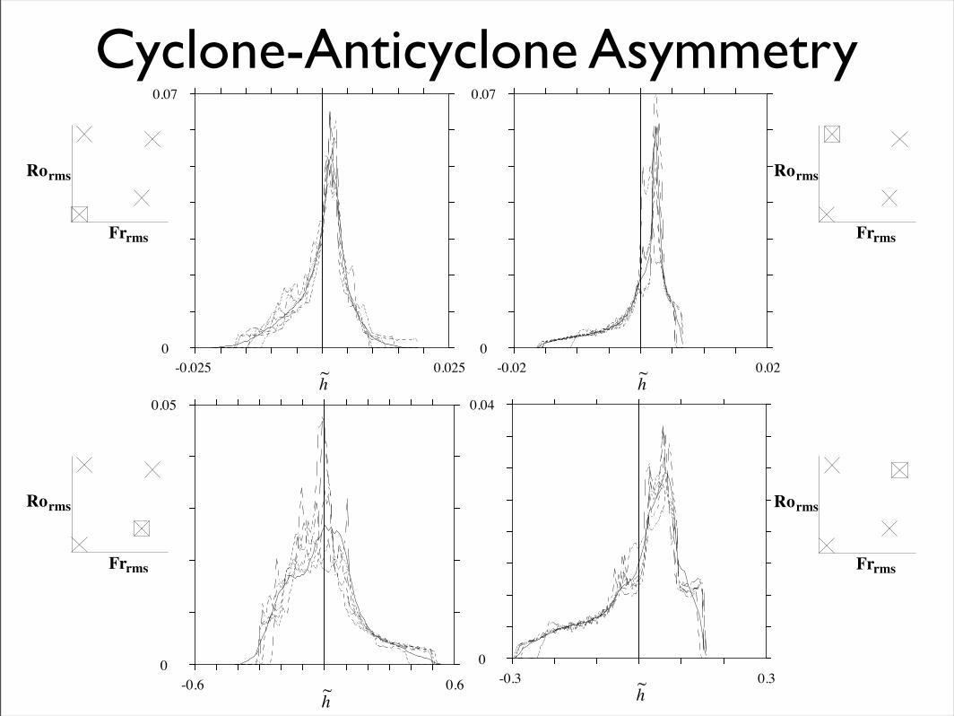
Figure 3.10: Probability density functions of depth h for the 4 cases. Dotted
lines show the distribution at t = 0, 10, 20, 30, 40 and the solid line shows the
time-mean distribution.
68
Case 1
h~-0.025 0.025
0
0.07
Case 2
h~-0.02 0.02
0
0.07
Case 3
h~-0.6 0.6
0
0.05
Case 4
h~-0.3 0.3
0
0.04
Figure 3.10: Probability density functions of depth h for the 4 cases. Dotted
lines show the distribution at t = 0, 10, 20, 30, 40 and the solid line shows the
time-mean distribution.
68
Frrms
Rorms
Frrms
Rorms
Frrms
Rorms
Frrms
Rorms
Cyclone-Anticyclone Asymmetry
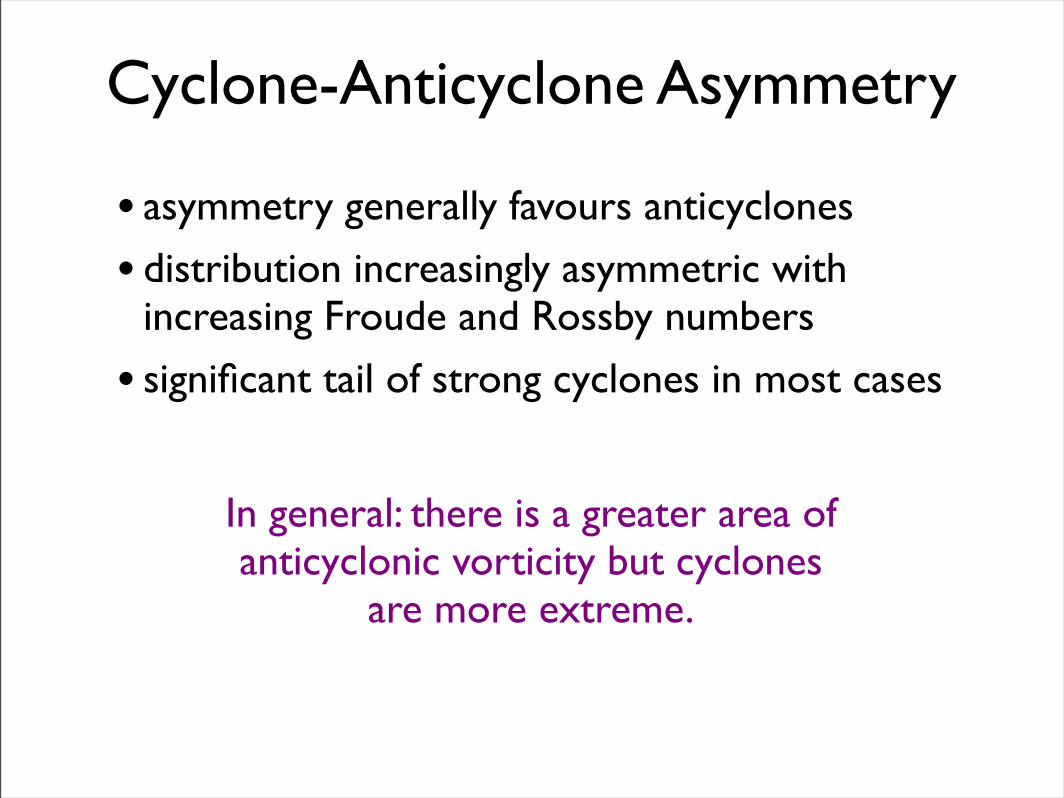
• asymmetry generally favours anticyclones
• distribution increasingly asymmetric with increasing Froude and Rossby numbers
• significant tail of strong cyclones in most cases
In general: there is a greater area of anticyclonic vorticity but cyclones
are more extreme.
Potential Vorticity Homogenisation
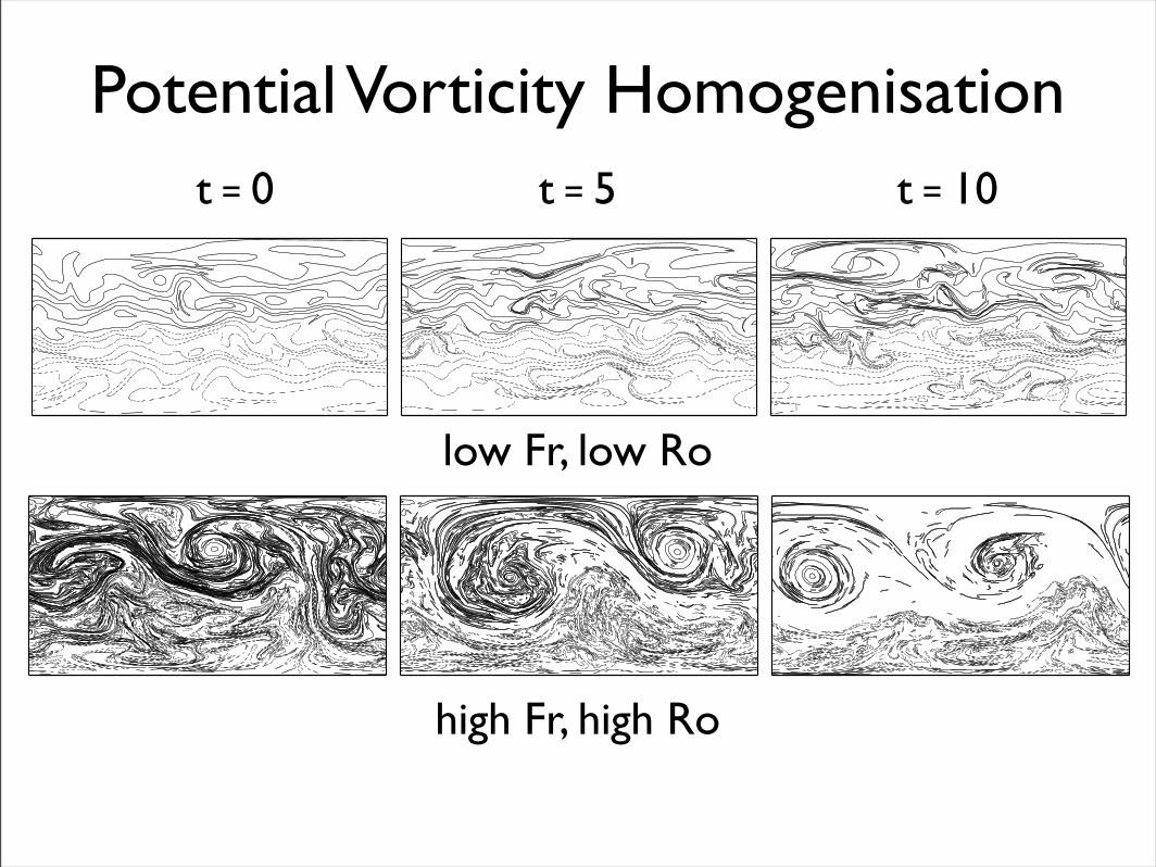
Figure 3.6: Evolution of ! (top row), h (second row), !/(2") (third row) fields
for case 1, shown at times t = 0, 5, 10. The contour interval is 0.002 for h, 0.0005
for !/(2") and 0.005 for "/(2")2.
62
Figure 3.9: Evolution of ! (top row), h (second row), !/(2") (third row) fields
for case 4, shown at times t = 0, 5, 10. Only every 8th contour of the PV field is
plotted. The contour interval is 0.02 for h, 0.01 for !/(2") and 0.5 for "/(2")2.
49
low Fr, low Ro
high Fr, high Ro
t = 0 t = 5 t = 10
Potential Vorticity Homogenisation
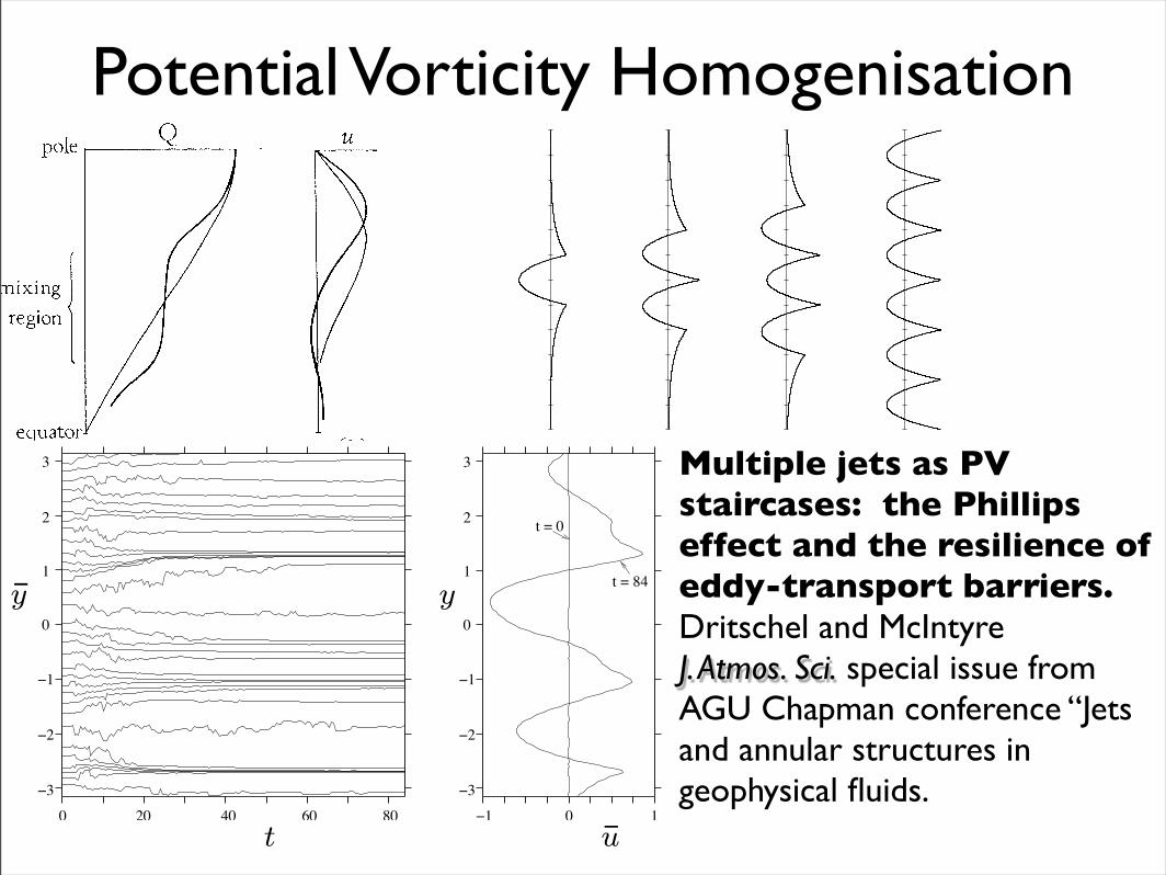
Figure 1: Schematic from McIntyre (1982), suggesting the robustness of nonlinearjet-sharpening by inhomogeneous PV mixing. Here most of the mixing is on theequatorward flank of an idealized stratospheric polar-night jet, in a broad midlatitude“surf zone” due to the breaking of Rossby waves arriving from below. The profilescan be thought of as giving a somewhat blurred, zonally-averaged picture. The lightand heavy curves are for conditions before and after the mixing event, where “after”means “after the wave has largely decayed”. The di!erence between the two zonal-velocity curves on the right is dictated by inversion of the di!erence between thetwo PV curves on the left, like smoothed versions of Equation (5.1) and Figure 7bsince over several scale heights the middle stratosphere behaves qualitatively likea shallow-water model with LD roughly of the order of 2000 km (Robinson 1988;Norton 1994). Vortex stretching associated with the horizontally-narrowing jet scaleincreases the relative vorticity at the pole (e.g., Dunkerton et al. 1981, Figures 4,5). Angular momentum is reduced even though the jet is sharpened. Long-rangeradiation stresses cannot be neglected. For Jovian and terrestrial-ocean jets, withtheir relatively smaller latitudinal scales, the mixing is typically strong on both sidesof each jet (e.g., Marcus 1993; Hughes 1996). In the Jovian case the mixing is almostcertainly due to a di!erent stirring mechanism altogether, namely, convection in theplanet’s interior; see footnote 4 and Section 8.
27
3
2
1
0
!1
!2
!3
0 20 40 60 80
3
2
1
0
!1
!2
!3
!1 0 1
t = 0
t = 84
y y
t u
Figure 6: dummy text
Figure 6: Diagnostics for the experiment of Figure 5. The left-hand panel showsthe time evolution of the zonal-mean position y(q, t) of each PV contour that wrapsthe domain, i.e. that closes on itself only through the periodic boundaries x =±!. The latitudinal coordinate y is in units of LD, and time t is in units of4!/|q!|max. PV mixing (in which the turbulent dissipation of fine-grain PV gradientsis achieved here by contour surgery) changes y(q, t) in time, here leading to a highlyinhomogeneous distribution of positions y at late times, as expected from the positive-feedback heuristic. Broadly speaking, the bunching of curves corresponds to eastwardjet formation and the spreading of curves to westward jet formation. The right-handpanel shows the zonally averaged zonal velocity u(y, t) at the initial and final timest = 0, 84. See remark at the end of Section 7. The inhomogeneous PV mixinghas produced three strong eastward jets, two of them sharply peaked in the mannercharacteristic of well developed eddy-transport barriers in a shallow-water system,with PV distributions close to jump discontinuities. Such PV distributions invertto velocity profiles locally resembling the idealized forms shown in Figure 7, whichcorrespond to perfectly sharp PV jump discontinuities.
32
Multiple jets as PV staircases: the Phillips effect and the resilience of eddy-transport barriers.Dritschel and McIntyreJ. Atmos. Sci. special issue from AGU Chapman conference “Jets and annular structures in geophysical fluids.
Figure 7: Idealized mass and velocity profiles for perfect PV staircase steps, asdetermined by PV inversion. Tick marks are at intervals of y = b = LD. From left toright, the first two profiles are for a single step or mixed zone, respectively the massshift or surface-elevation change given by (5.2)!. and the velocity profile given by(5.1)!. The remaining profiles are the velocity profiles for two, three and an infinitenumber of perfect steps, the last from Eq. (5.3) shifted by b. Note that the angularmomentum changes required to form these staircase structures are nonvanishing, andare precisely dictated by the PV inversions, or equivalently by Eq. (7.2).
33
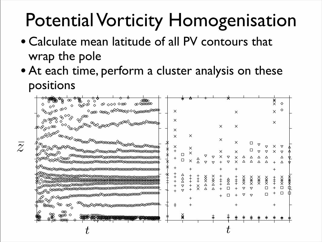
Potential Vorticity Homogenisation• Calculate mean latitude of all PV contours that
wrap the pole• At each time, perform a cluster analysis on these
positions3
2
1
0
!1
!2
!3
0 20 40 60 80
3
2
1
0
!1
!2
!3
!1 0 1
t = 0
t = 84
y y
t u
Figure 6: dummy text
Figure 6: Diagnostics for the experiment of Figure 5. The left-hand panel showsthe time evolution of the zonal-mean position y(q, t) of each PV contour that wrapsthe domain, i.e. that closes on itself only through the periodic boundaries x =±!. The latitudinal coordinate y is in units of LD, and time t is in units of4!/|q!|max. PV mixing (in which the turbulent dissipation of fine-grain PV gradientsis achieved here by contour surgery) changes y(q, t) in time, here leading to a highlyinhomogeneous distribution of positions y at late times, as expected from the positive-feedback heuristic. Broadly speaking, the bunching of curves corresponds to eastwardjet formation and the spreading of curves to westward jet formation. The right-handpanel shows the zonally averaged zonal velocity u(y, t) at the initial and final timest = 0, 84. See remark at the end of Section 7. The inhomogeneous PV mixinghas produced three strong eastward jets, two of them sharply peaked in the mannercharacteristic of well developed eddy-transport barriers in a shallow-water system,with PV distributions close to jump discontinuities. Such PV distributions invertto velocity profiles locally resembling the idealized forms shown in Figure 7, whichcorrespond to perfectly sharp PV jump discontinuities.
32
3
2
1
0
!1
!2
!3
0 20 40 60 80
3
2
1
0
!1
!2
!3
!1 0 1
t = 0
t = 84
y y
t u
Figure 6: dummy text
Figure 6: Diagnostics for the experiment of Figure 5. The left-hand panel showsthe time evolution of the zonal-mean position y(q, t) of each PV contour that wrapsthe domain, i.e. that closes on itself only through the periodic boundaries x =±!. The latitudinal coordinate y is in units of LD, and time t is in units of4!/|q!|max. PV mixing (in which the turbulent dissipation of fine-grain PV gradientsis achieved here by contour surgery) changes y(q, t) in time, here leading to a highlyinhomogeneous distribution of positions y at late times, as expected from the positive-feedback heuristic. Broadly speaking, the bunching of curves corresponds to eastwardjet formation and the spreading of curves to westward jet formation. The right-handpanel shows the zonally averaged zonal velocity u(y, t) at the initial and final timest = 0, 84. See remark at the end of Section 7. The inhomogeneous PV mixinghas produced three strong eastward jets, two of them sharply peaked in the mannercharacteristic of well developed eddy-transport barriers in a shallow-water system,with PV distributions close to jump discontinuities. Such PV distributions invertto velocity profiles locally resembling the idealized forms shown in Figure 7, whichcorrespond to perfectly sharp PV jump discontinuities.
32
!!!!!!
!!!!!!!
!!!!!
DCi
ri
rimi
d(Ci+1, Ci+2)
Ci
z1i
zni
i
Ci+1
Ci+2
uij
z
Figure 3.14: Schematic illustrating some of the cluster notation summarised in
table 3.3. The crosses show the position of the data at one particular time.
78
Potential Vorticity Homogenisation
0
0.02
0.04
0.06
0.08
0.1
0 0.2 0.4 0.6 0.8 1.0
Frrms
! rms
0
0.02
0.04
0.06
0.08
0.1
0 1 2 3 4
Rorms
! rms
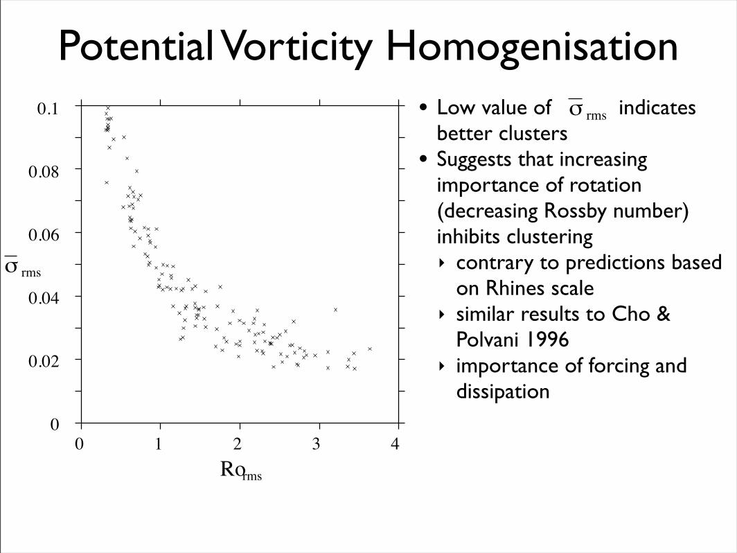
Figure 3.17: !rms versus Fr (left hand figure) and versus Ro (right hand figure)
Remember that small values of !rms indicate well clustered contours.
will indicate local tightening of PV contours which is exactly what we expect to
find in westerly jets. Figures 3.18-3.21 show the time evolution of P for the four
cases. We plot the scaled palinstrophy (log10(P/(3!Prms)) in order to highlight
the areas with the steepest gradients. Also plotted is the spatial distribution of
the Froude number which indicates where the inertia-gravity wave speed is fast
compared to the flow speed. Note that the times shown are t = 0, 5, 10, 20 and 40
so that the first 4 figures show the early evolution during which the adjustment
is occurring and the final figure shows the long term behaviour.
Structures in the plots of the local Froude number and the palinstrophy field
are closely correlated although, since the Froude number depends on the global
distribution of PV, it is smoother and does not reveal the smaller scale features
evident in the palinstrophy plots. Since the jets meander, it may be that a
significant component of the local flow is in the cross-jet direction and this may
mask the presence of strong flow along the jet axis in the Froude number plots.
The palinstrophy plots su!er from no such di"culties. The detailed structure
evident in these plots enables us to precisely locate the jet axes as the regions
where the PV gradient is strongest (see the dark regions in the palinstrophy plots,
84
• Low value of indicates better clusters
• Suggests that increasing importance of rotation (decreasing Rossby number) inhibits clustering‣ contrary to predictions based
on Rhines scale‣ similar results to Cho &
Polvani 1996‣ importance of forcing and
dissipation
0
0.02
0.04
0.06
0.08
0.1
0 0.2 0.4 0.6 0.8 1.0
Frrms
! rms
0
0.02
0.04
0.06
0.08
0.1
0 1 2 3 4
Rorms
! rms
Figure 3.17: !rms versus Fr (left hand figure) and versus Ro (right hand figure)
Remember that small values of !rms indicate well clustered contours.
will indicate local tightening of PV contours which is exactly what we expect to
find in westerly jets. Figures 3.18-3.21 show the time evolution of P for the four
cases. We plot the scaled palinstrophy (log10(P/(3!Prms)) in order to highlight
the areas with the steepest gradients. Also plotted is the spatial distribution of
the Froude number which indicates where the inertia-gravity wave speed is fast
compared to the flow speed. Note that the times shown are t = 0, 5, 10, 20 and 40
so that the first 4 figures show the early evolution during which the adjustment
is occurring and the final figure shows the long term behaviour.
Structures in the plots of the local Froude number and the palinstrophy field
are closely correlated although, since the Froude number depends on the global
distribution of PV, it is smoother and does not reveal the smaller scale features
evident in the palinstrophy plots. Since the jets meander, it may be that a
significant component of the local flow is in the cross-jet direction and this may
mask the presence of strong flow along the jet axis in the Froude number plots.
The palinstrophy plots su!er from no such di"culties. The detailed structure
evident in these plots enables us to precisely locate the jet axes as the regions
where the PV gradient is strongest (see the dark regions in the palinstrophy plots,
84
Cluster Analysis Issues
• input parameters for clustering algorithms
• constraint that PV contours must wrap sphere‣ precession of polar vortices
• latitudinal averaging‣ meandering of jets
Complex structure of jets defies simple classification - instead a more
local examination is required.
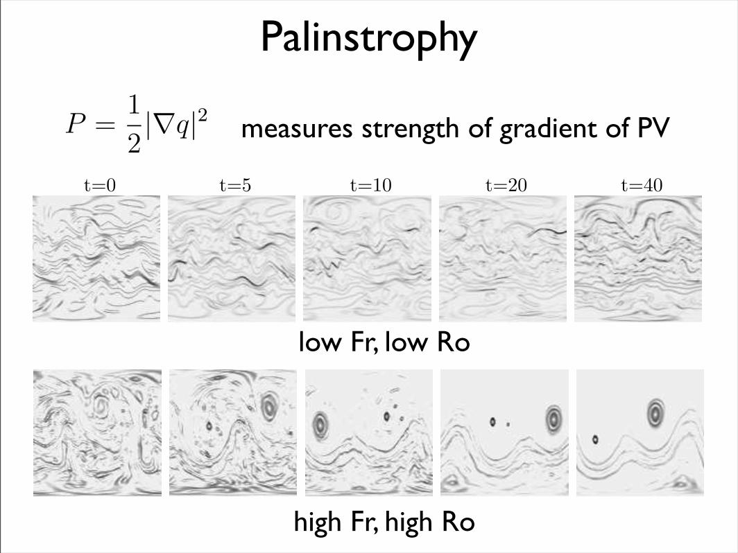
Palinstrophy
t=0 t=5 t=10 t=20 t=40
t=0 t=5 t=10 t=20 t=40
Figure 3.18: Evolution of palinstrophy (top) and local Froude number (bottom)
for case 1. For each figure the range has been determined to optimise the detail
shown in the figure so these figures are for qualitative rather than quantitative
comparison. Note also that the figures are not evenly spaced in time.
interaction between the jets and the vortices produces strongly meandering jets
that then inhibit the merger of the two remaining northern hemisphere vortices
which are trapped in the meanders of the jet.
86
t=0 t=5 t=10 t=20 t=40
t=0 t=5 t=10 t=20 t=40
Figure 3.21: Evolution of palinstrophy (top) and local Froude number (bottom)
for case 4. For each figure the range has been determined to optimise the detail
shown in the figure so these figures are for qualitative rather than quantitative
comparison. Note also that the figures are not evenly spaced in time.
88
high Fr, high Ro
low Fr, low Ro
measures strength of gradient of PV
both to the precession of the ‘polar’ vortices and to the nature of the clustering
algorithm which is, despite all our e!orts, very sensitive. A more robust measure
appears to be the average value of the validity index over the last 10 days of
each simulation. This number tells us if the validity index perceives the PV
contours to be well clustered or not. Unsurprisingly, given the results in table
3.4, the r.m.s. standard deviation gives the most informative results. Figure
3.17 shows !rms versus Frrms (on the left) and versus Rorms (on the right). We
see that there is a slight correlation between !rms and Fr, with the PV contours
becoming more clustered with increased Froude number. However, the correlation
between !rms and Ro is striking. !rms decreases with increasing Ro, levelling out
at around Ro = 2. This suggests that increasing the importance of rotation
(i.e. smaller Rossby number) inhibits the clustering of PV contours. This seems
counter intuitive and is contrary to predictions based on the Rhines scale, but
Cho and Polvani [1996] find that a similar result emerges from their spherical
simulations. They suggest that the variation of " with latitude coupled with the
lack of forcing, causes the jets to be ill defined. They note that the only obvious
strong jets are those surrounding the polar vortices and, as mentioned above, the
polar vortices pose a problem for our method since they rarely sit neatly over the
pole.
Two factors seriously inhibit the performance of the clustering approach: the
constraint the PV contours must wrap the sphere and the latitudinal averaging.
The first causes the strong jets around the ‘polar’ vortices to be neglected, the
second smears out the complex longitudinal structure of the jets. We have found
that a local analysis of the jet characteristics is much more revealing. This can
be achieved by examining the palinstrophy field
P =1
2|!q|2, (3.16)
which measures the strength of the gradient of the PV. A large palinstrophy value
83
Conclusions
• Explored new ways of looking at cyclone-anticyclone asymmetry and jet formation.
• Cyclone-anticyclone asymmetry
• favours anticyclones
• asymmetry increases with both Froude and Rossby number
• significant tail of extreme cyclones
• Jet formation
• cluster analysis misses complexity of jets
• palinstrophy field reveals jet structure