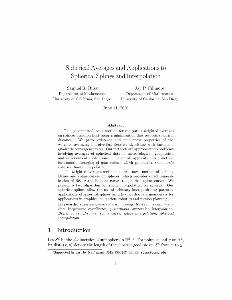
Spherical Averages and Applications to

Spherical Splines and Interpolation

Samuel R. Buss∗

Department of MathematicsUniversity of California, San Diego

Jay P. FillmoreDepartment of Mathematics

University of California, San Diego

June 11, 2001

AbstractThis paper introduces a method for computing weighted averages

on spheres based on least squares minimization that respects sphericaldistance. We prove existence and uniqueness properties of theweighted averages, and give fast iterative algorithms with linear andquadratic convergence rates. Our methods are appropriate to problemsinvolving averages of spherical data in meteorological, geophysicaland astronomical applications. One simple application is a methodfor smooth averaging of quaternions, which generalizes Shoemake’sspherical linear interpolation.

The weighted averages methods allow a novel method of definingBezier and spline curves on spheres, which provides direct general-ization of Bezier and B-spline curves to spherical spline curves. Wepresent a fast algorithm for spline interpolation on spheres. Ourspherical splines allow the use of arbitrary knot positions; potentialapplications of spherical splines include smooth quaternion curves forapplications in graphics, animation, robotics and motion planning.Keywords: spherical mean, spherical average, least squares minimiza-tion, barycentric coordinates, quaternions, quaternion interpolation,Bezier curve, B-spline, spline curve, spline interpolation, sphericalinterpolation.

1 Introduction

Let Sd be the d-dimensional unit sphere in Rd+1 . For points x and y on Sd ,let distS(x, y) denote the length of the shortest geodesic on Sd from x to y .

∗Supported in part by NSF grant DMS-9503247. Email: sbuss@ucsd.edu

1

Let ||x− y|| denote the usual Euclidean distance between x and y in Rd+1 ;note ||x− y|| < distS(x, y) for any distinct points x and y on Sd .

Let p1, . . . , pn be points on Sd : the main purpose of the present paper isto define a weighted average or centroid of these n points using as weightsvalues w1, . . . , wn such that each wi ≥ 0 and and such that

∑i wi = 1. This

weighted average will be denoted

C = ©∑n

i=1wi · pi,

and is to be defined in terms of distances in Sd , using distS(−,−) insteadof Euclidean distance. Since Sd is not a linear space, it is not immediatelyobvious that there is a sensible way to define this weighted average; however,in section 2 below, we shall show that it makes sense to define the weightedaverage as the result of a least squares minimization, namely as the point Con Sd which minimizes the value

f(C) = 12

∑iwi · distS(C, pi)2.

This method of calculating the centroid C will be shown to enjoy a numberof nice properties: firstly, it is a natural analogue of weighted averagesin Euclidean space; secondly, it generalizes Shoemake’s spherical linearinterpolation, which provides a definition of a spherical average of twopoints; and thirdly, the centroid value C exists and is unique in manycommon situations. In section 3, we describe efficient methods of calculatingthe centroid C using iterative methods with linear and quadratic convergencerates.

To the best of our knowledge, this kind of weighted average or centroidon spheres has not been considered in the past. Indeed, there is an extensiveliterature on averaging points on spheres and on statistical analysis of pointsthat lie on spheres, e.g., see [34, 35, 1] or the book [37] and the references citedtherein. Most of that work performs the averages in Rd+1 and renormalizesto place the result on the sphere; namely, they compute the centroid as∑

i wipi

||∑i wipi||

with the summation being taken inside Rd+1 . Shoemake [30] noted that evenwhen taking weighted averages of only two points, this kind of renormalizedRd+1 -average causes undesirable effects. Shoemake used the quaternionrepresentation of rigid-body orientations as points on S3 to perform smoothinterpolation between two orientations of a rigid body in 3-space. He

2

pointed out that the renormalized Rd+1 -averaging method did not produceuniform interpolation of orientations and was therefore unsuitable for manyapplications: his solution was to use “spherical linear interpolation” or“slerp”-ing to compute the weighted average of only two points on the spherebased on geodesic length in S3 . Our spherical averaging method provides asmooth generalization of Shoemake’s spherical linear interpolation to allowcomputing weighted averages of more than two points.

A few authors consider statistics of spherical data that do not merelyembed the results in Rd+1 : for instance Clark and Thompson [6] performaverages using a stereographic projection (the axis for the stereographicprojection is calculated by averaging in Rd+1 ) — this suffers from distorsionfor data points located away from the center of projection. Later, in [33],they used averages based on longitude and latitude values: this causesdistorsion for data located away from the equator.

A number of authors, including [3, 14, 39], have considered averages infairly general metric space and Banach space settings. These settings aretoo general to be applicable to averages on the sphere Sd .

Spherical splines. The second main topic of the present paper is thethe application of spherical averaging to generate spline curves on spheres.Spherical spline curves have potential applications in computer graphics, inanimation and in robotics and motion planning based on quaternions.

In the Euclidean case, a spline consists of control points p1, . . . , pn (inRd+1 , say) and of blending functions f1(t), . . . , fn(t) (also called “basisfunctions”) defined for t in the domain [a, b] for some a < b . The functionsfi have the property that, for all t ∈ [a, b] ,

f1(t) + f2(t) + · · ·+ fn(t) = 1, and fi(t) ≥ 0, for all i . (1)

In the most common applications, the functions fi(t) are defined by specify-ing knot positions t1, . . . , tk+d and constructing the blending functions fi(t)from the knot positions. This provides a framework for defining blendingfunctions which give curves with desired smoothness properties, and evensharp bends or cusps where desired (see e.g., [10]). Once the blendingfunctions have been defined, the spline curve is defined by

s(t) = f1(t)p1 + f2(t)p2 + · · ·+ fn(t)pn.

This gives a curve parameterized by t .Generalizing this approach to spline curves to the d-sphere Sd becomes

straightforward after the development of spherical averages in sections

3

2 and 3 below. Namely, let the control points p1, . . . , pn lie on Sd . Givenblending functions fi(t) which satisfy (1), a spline curve on the sphere canbe defined by using the spherical weighted average:

s(t) = ©∑n

i=1fi(t) · pi.

In this way, many of the techniques of defining B-splines in Euclidean spaceare generalized to the sphere. As a special case, this allows the definition ofspherical analogues of piecewise cubic B-spline curves.

Spherical spline interpolation. The control points used to define a splinecurve typically do not lie on the resulting curve. However, one often wishesto use spline curves to interpolate points, i.e., one has points q1, . . . , qn andhas n distinct time values t1, . . . , tn and one wishes to ensure that s(ti) = qi

for all 1 ≤ i ≤ n . There are a variety of well-known approaches for pickingblending functions fi so as to ensure the spline has the desired smoothnessproperties and to control the behavior of the spline curve at its endpoints.Given the interpolation points qi and the time values ti and the blendingfunctions fi , one then needs to find control points p1, . . . , pn which causethe curve to interpolate the points qi .

For curves on the sphere, this means choosing points pi on Sd so that

qj =n

©∑i=1

fi(tj) · pi for 1 ≤ j ≤ n .

In most common applications (where one generates spline curves whichare piecewise degree 3 polynomials), the values fi(tj) are non-zero only forj ∈ {i−1, i, i+1} . Therefore in the Euclidean case, the control points pi canbe found very simply by solving a tridiagonal matrix equation. The matrixcannot be so simply inverted for spherical spline interpolation; instead weuse an iterative procedure to determine p1, . . . , pn . Two such procedures aredescribed in section 4.2, and experimental results show them to be quite fastin practice. Indeed, in realistic small examples, the pi ’s can be found in a fewmilliseconds or less — section 5 lists a variety of experimental measurementsof runtime.

Prior work. There has been extensive prior work on spherical splines; wesurvey here a major portion of it, with an eye to how our methods improveon the prior methods.

The earliest description of spherical spline interpolation was by Parker-Denham [25], who described spherical splines on Sd by defining a spline

4

curve in Rd+1 and normalizing to map the curve to the sphere. Since thecurve may deviate a long way from the sphere, the normalization process ismathematically unnatural and can cause significant distorsion.

Thompson and Clark [33] (see also the references cited therein) appliedspherical spline curves to the problem of determining the Gondwananapparent polar wonder path to study the past movements of continents. Theydefined spherical spline curves following a method of Gould by interpolatingin latitude and longitudinal space. This method causes distorsion nearthe poles. Fisher-Lewis [11] proposed interpolating points on Sd with asmooth curve by combining smooth segments so as to ensure continuoussecond derivatives and suggested using either third-order natural splines orloxodromes.

Spherical splines on the 3-sphere S3 , the unit sphere in R4 , havebecome quite important in computer graphics and animation because ofthe correspondence between orientations of solid bodies and quaternions(see [7, 30]). Quaternions can be viewed as (pairs of antipodal) points on S3

and thus spherical spline curves can be used to specify a smooth transitionof solid orientations. Shoemake [30, 31] was the first apply quaternionsto graphics and animation: he stressed the importance of using sphericaldistance instead of Euclidean distance. In [30] he introduced the now widelyused method of spherical linear interpolation (“slerping”) for two points. Healso used analogues of the de Casteljau method of calculating Bezier curvesto define curves on the sphere, and in [31] introduced a similar, but fastermethod called Squad. A number of other authors have proposed similarmethods, also based on Catmull-Rom splines: these methods allow a generalspline to be defined in terms of multiple linear interpolations between pairsof points and in this way slerping can be used to define higher-order sphericalsplines. Duff [9] gives the most in-depth development of this kind of methodand proves a variation diminishing property for these splines. A disadvantageto these methods on the sphere, at least as described in the extant literature,is that they work well only for equally spaced knot positions. However, itshould be possible to give more sophisticated spherical spline curves based onthe de Castaljau method which are computed using multiple slerps betweenpairs of points and which work well for arbitrary knot positions (indeed,knot insertion methods for spline curves should suffice for this, c.f. [10]).Moreover, these methods should give curves satisfying the properties a.-f.below. These kinds of algorithms, however, would suffer from the fact thatresulting curve would depend on the details of the order in which slerps areperformed: for instance, the results of repeated knot insertion would dependon the order in which the knot were inserted. By contrast, spline curves

5

based on our spherical averages provide a mathematically natural way ofblending multiple control points in a single step without having to arbitrarilychoose an order for averaging.

Wang-Joe [36] suggest forming smooth spherical curves which arepiecewise small circles. A more sophisticated approach was taken byRoberts-Bishop-Ganapathy [29] and Kim-Nam [20, 21] who proposed defin-ing interpolating splines using spline segments which are obtained byblending small circles on the sphere. This method provides nice smoothnessproperties, but performs poorly when data points are not equally spaced,and does not allow specification of knot positions.

Ge-Ravani [13] and Juttler [17] suggest the use of dual quaternioncurves to control solid body orientation and position simultaneously. Thesubsequent paper of Juttler-Wagner [18] uses piecewise rational functionsfor the entries of orientation matrices; this method suffers from havingcontrol points which are only affine (non-orthogonal) matrices, More recently,Alfeld et al. [1] discuss defining barycentric coordinates and spherical splinefunctions with good continuity properties using renormalized-Rd methods.In all four of these papers, the interpolation methods are not intrinsic to thesphere in the sense of respecting spherical distance.

Kim-Kim-Shin [19] give a method of constructing quaternions curves byusing general blending functions. Like our method introduced in this paper,they allow the use of arbitrary blending functions and thus arbitrarily spacedknots and control points. Their use of blending functions is mathematicallyquite different from ours: instead of using a general method of computingweighted averages on the sphere, they compose a series of rotations basedon slerps between the control points. This is mathematically somewhatunnatural; for instance, reversing the order of the control points can alterthe spline curve. Another undesirable feature is that their spline curvesmay not satisfy the “convex hull” property; for instance it is possible forthe control points to lie on vertices of a triangle in a hemisphere and forthe spline curve to lie partly outside the triangle. In addition they do notaddress the problem of interpolation. Nonetheless, their spline curves enjoymany of the advantages we list below for our spherical splines, particularlyif the control points are not very widely spaced and if the blending functionshave sufficiently local support.

Gabriel-Kajiya [12], Jupp-Kent [16], Noakes-Heinzinger-Paden [23],Park-Ravani [24], and Dam-Koch-Lillhom [8] proposed using natural splineswhich minimize covariant (tangential) acceleration. The first paper [12] gavea very general method which works on any manifold as well as described thespecialization of their method to the sphere. Curves obtained by minimizing

6

covariant acceleration have nice smoothness, but suffer from not havinglocal control, since changing one control point changes the whole curve. Inaddition, they are computationally somewhat difficult; e.g., [12] report thatit takes a “few tens of seconds” to find an interpolating spline curve on anIBM 4341. Barr et al.[4] proposed minimizing covariant accelerations whilerelaxing the requirement that the curve lie exactly on the sphere, because thisallowed faster computation. They noted that a curve could be computed in“a few minutes per interpolation”; although later [28] characterized the runtime of [4] as “several minutes to hours.” Ramamoorthi-Barr [28] describea numerically fast algorithm that can get close to an optimal curve withinabout 4 seconds (machine type and programming language unspecified).This run time is quite adequate for interactive applications, but unlike ouralgorithms is not fast enough for real-time applications. Like other naturalspline methods, the spline curves of [4, 28] do not allow local control or(without some kind of modification of their energy functions) specificationof knot positions. Their curves lie close to, but not on, the 3-sphere andhave to be normalized to lie on the sphere. The papers [40, 24] suggest usingcurves that minimize covariant acceleration and/or jerk. [40] give closedform solutions for special cases of the two point interpolation problems, e.g.,when the initial and final velocity are both zero; [24] give approximationsthat work well in restricted cases, e.g., when the initial and final rotation arenot too different, and give applications to interpolation with knot positions.

The definition of spherical splines and spherical spline interpolation inthe present paper provides several advantages:

a. It allows construction of spherical splines with non-interpolated controlpoints, and also allow interpolating curves by suitably choosing controlpoints.

b. They can be computed fast enough for some real-time applications:see section 5 for details.

c. The spherical averages and spherical splines are invariant underrotations of the sphere; there is no distorsion near the poles for instance.

d. The algorithms are completely intrinsic to the sphere: we do notcompute averages in Euclidean space and then renormalize back to thesphere. Spherical distances, not Euclidean distances, are the basis foraveraging and blending. The spherical weighted averages are mathematicallynatural. If the points all lie on a geodesic (great circle), then our algorithmscorrespond to weighted averages on a line, but using geodesic arc length.

7

e. The spline curve lies in the convex hull of the control points.f. Since our spline curves are defined in terms of weighted averages

of spherical data, the well-known methods for generating spline curves inEuclidean space immediately generalize to the sphere. This immediatelygives several advantages which carry over from the Euclidean case. First,the well-known strategies for choosing knot positions can now be appliedto spherical splines to control the smoothness of the curve. It is thereforeeasy to define spherical splines with any number of continuous derivatives.Second, knot positions need not be equally spaced or distinct. This allowsdefining spline curves with sharp localized bends and even discontinuousderivatives if desired. Third, spherical splines can be defined with localcontrol; i.e., changing one control point can affect the curve only in segmentsclose to the control point.

The outline of the rest of the paper is as follows. Section 2 gives themathematical definition of spherical weighted averages and includes proofsof existence and uniqueness. Section 2 also establishes smoothness of thespherical weighted average as a function of the weights and the points pi ,and proves a convexity property for spherical weighted averages. Only thefirst part of section 2 is needed for the rest of the paper: the reader is whois interested more in implementation than in mathematical proofs, may skipsections 2.1 through 2.3. Section 3 describes two algorithms for computingspherical weighted averages. Section 4 describes applications to sphericalspline curves and to spherical spline interpolation. Section 5 describes theexecution speed of our algorithms and compares them to other approaches.We conclude with some open problems in section 6.

2 Spherical Weighted Averages

We consider the following problem: given n points p1, . . . , pn lying on thesphere and n non-negative real weights w1, . . . , wn with sum equal to 1, andwe wish to define a weighted average function

Avg(w1, p1; w2, p2; . . . wn, pn) = ©∑

iwi · pi (2)

which computes a point on the sphere which is a “weighted average” ofthese given n points. This kind of problem is important for a number ofapplications including statistics of spherical valued functions (as might arisein astronomical, geophysical, meteorological applications), and applicationsto solid body orientations (quaternions), etc. There are a number of natural

8

properties the Avg function should satisfy: (1) the averaging should beintrinsic to the sphere, and depend on spherical distances, not Euclideandistances, between points on the sphere, (2) in the degenerate case wherethe points pi lie on a geodesic in a hemisphere, the weighted average shouldbe computed in the usual fashion based on distances along the geodesic,(3) the value of Avg should be a C∞ -continuous function of the weights wi

and the points pi , at least in the case when all the points are containeda hemisphere of the sphere. When averaging quaternions, condition (2)states that the average of two points on the 3-sphere should corresponds toShoemake’s slerping algorithm. A final condition is that the Avg functionshould act qualitatively like a weighted average.

It is not possible to directly define the Avg as a linear combination ofthe points p1, . . . , pn and respect geodesic distance on the sphere. However,there is an alternative definition of Euclidean weighted sums that can beadapted to the sphere. Letting ||p − q|| denote the Euclidean distancebetween points p and q , the Euclidean weighted average

w1p1 + w2p2 + · · ·+ wnpn

can be defined as the point q which minimizes the value of the function

f(q) = 12

∑n

i=1wi||q − pi||2.

In other words, in Euclidean space, the weighted average of the points pi isequal to the point where a weighted sum of squares of distances is minimized.To prove this fact, let the Euclidean space be Rd , and each pi be in Rd andq range over points in Rd : let the k -th component of q and of pi be denotedqk and pi,k , respectively (1 ≤ k ≤ d). By the Pythagorean theorem,

f(q) = 12

∑i,k

wi(qk − pi,k)2.

Differentiating with respect to qk , any critical point of f must satisfy∑n

i=1wi(qk − pi,k) = 0,

whence, using the fact that the weights sum to 1, there is a unique criticalpoint and it is given by

qk =∑n

i=1wipi,k.

It is clear that this critical point is a global minimum and of course it is theweighted average of the points pi .

9

To transfer the least squares minimization to the sphere, we let distS(p, q)denote the spherical distance from points q and p on the d-sphere, namely,the length of the shortest geodesic seqment from q to p . Now let thefunction f be defined on the d-sphere by

f(q) = 12

∑n

i=1wi · distS(q, pi)2. (3)

We thus define the value of Avg(w1, p1; . . . wn, pn) to be the point q on Sd

which minimizes f(q). Since the notation Avg is fairly inconvenient andnon-intuitive, we henceforth use in its place the modified summation notation

©∑n

i=1wi · pi

where the new summation symbol means that it is not a traditional sum, butinstead represents the value minimizing equation (3). Sometimes, we use asuperimposed ‘+’ and small circle to represent the same quantity, namely,we sometimes denote ©

∑ni1

wi · pi by

w1 · p1 ◦+ w2 · p2 ◦+ · · · ◦+ wn · pn

This modified summation and addition notation is suggestive, butthe reader should be aware that many common properties of ordinarysummations are not shared by spherical weighted averages; for instance,it is usually the case that the values 2

3 · (12 · p1 ◦+ 1

2 · p2) ◦+ 13 · p3 and

13 · p1 ◦+ 2

3 · (12 · p2 ◦+ 1

2 · p3) are distinct. This failure of associativity is anexample of how our weighted average Avg differs from using progressiveslerping, that is to say, the Avg value cannot be computed by takingsuccessive spherical averages of pairs of points. Indeed, by Brown andWorsey [5], there is no way to define spherical averages which is intrinsic tothe sphere so that associativity holds.

Fix points pi on the d-sphere Sd and non-negative weights wi with sumequal to 1 and let f be the weighted sum of squares of spherical distances (3).By the compactness of the sphere, the function f has a minimum value: inorder for the weighted average ©

∑i wi · pi to be well-defined, the function f

must have attain its minimum value at a unique point on Sd . Of coursethis condition may not always hold; for instance if the points p1, p2, p3 areequally spaced around the equator of S2 and if w1 = w2 = w3 = 1/3, thenf is minimized at both the north and south poles. As another example, ifthere are six equally weighted points on S2 distributed at the intersectionsof S2 with the x, y, z -axes, then f attains its minimum value at the eightpoints (±1/

√3,±1/

√3,±1/

√3).

10

However, in many situations the function f does attain a uniqueminimum: the easiest case, treated in the next theorem, is when the points pi

all lie in a common hemisphere of Sd (by convention, a hemisphere is alwaysclosed). By a ‘critical point’, we mean a point where the first derivativesof f are all zero.

Theorem 1 Suppose the points p1, . . . , pn all lie in a hemisphere H of Sd ,with at least one point pi in the interior of H with wi 6= 0. Then thefunction f has a single critical point q in H , and this point q is the globalminimum of f .

It will be clear from the proof that the assumption that the points all lie ina single hemisphere can be relaxed significantly. Theorem 5 states examplesof other conditions that imply the uniqueness of a global minimum for f .

Before we prove Theorem 1, we introduce the exponential and logarithmicfunctions, and derive formulas for the partial derivatives of f : these will alsobe useful for the development of algorithms for spherical weighted averagesin section 3. The partial derivatives of f are with respect to displacementsin the sphere around a point q ∈ Sd . To make this formal, we define Tq

to be the hyperplane tangent to Sd at the point q . The hyperplane Tq isd-dimensional and can be coordinatized by letting the point q be the originof Tq and letting the axes of Tq be arbitrary orthonormal axes which aretangent to the sphere. We define the exponential map at q to be the mappingfrom the tangent hyperplane Tq to the sphere which preserves distances andangles from q .∗ To make this precise, we need to choose an appropriate setof coordinates for Tq and Rd+1 . Let points in the space Tq be specified usingcoordinates x1, . . . , xd (so that the point q is the origin). Let x′1, . . . , x′d+1

be the coordinate axes for Rd+1 . Without loss of generality (choose new axesfor Rd+1 if necessary), the point q is at the point (0, . . . , 0, 1) in Rd+1 andthe axes x′i are parallel to xi for all i ≤ d . The exponential map is denotedexpq(·) and is a function mapping a point p with coordinates (x1, . . . , xd)to the point expq(p) = (x′1, . . . , x′d+1) where

x′i = xi · sin r

r

for 1 ≤ i ≤ d , where r =√∑

x2i is the distance from q to p , and x′d+1 =

cos r . We let (sin 0)/0 equal 1, and thus expq(q) = q . Furthermore, since

∗The terminology “exponential map” comes from Lie theory; this paper does notdepend on knowledge of Lie theory however. The exponential map has been discussed inthe setting of computer graphics by Hart et al. [15] and Dam et al. [8].

11

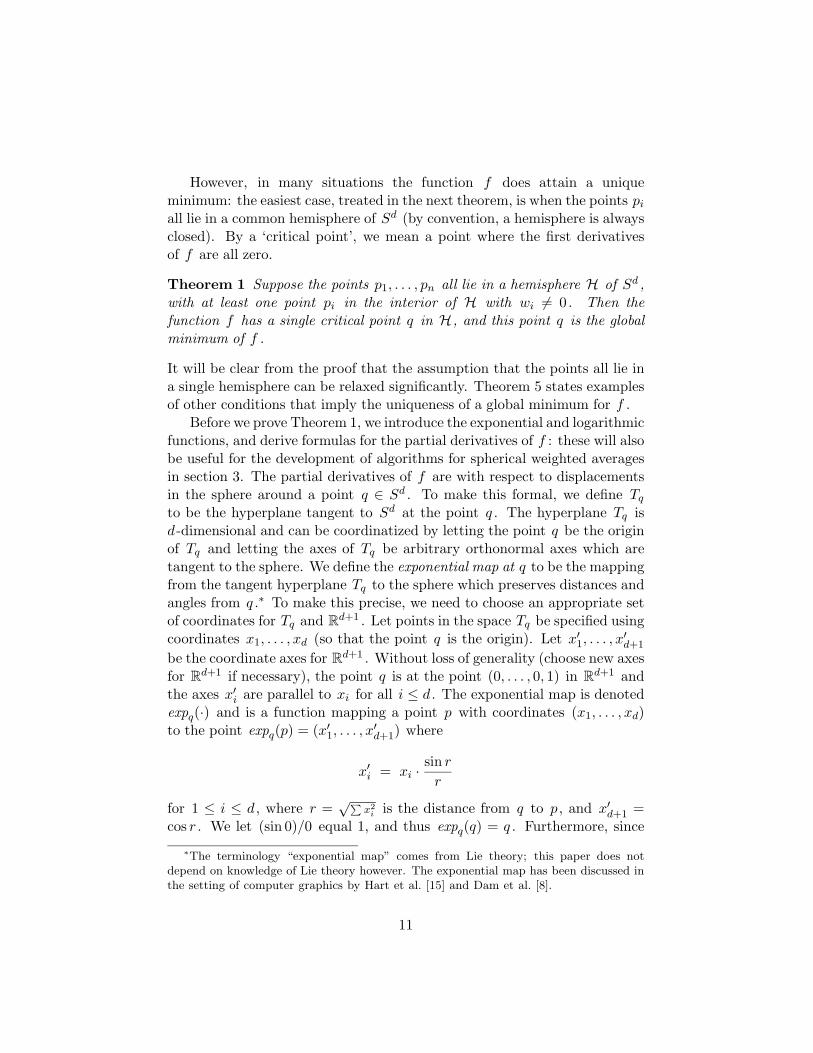
the sphere has unit radius, it is clear that r is equal to the spherical distancefrom q to expq(p) provided r ≤ π . Thus the exponential map takes pointsin the tangent plane to points on the sphere, preserving distance from q ;it also preserves the tangential direction from q . Actually, to be precise,the exponential map only preserves angles and distances for points in thetangent plane which have distance < π from q ; however, we shall implicitlyassume this condition holds whenever it is needed.

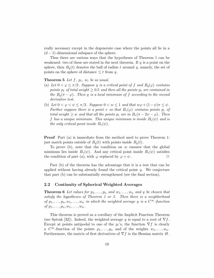
q pr

expq(p)r

Figure 1: The exponential map preserves distances < π and directionsfrom q

The inverse of the exponential map is denoted `q(p) and it maps a point pon Sd to the tangent hyperplane, provided p is not antipodal to q . We haveexpq(`q(p)) = p and the formula governing the inverse map is

xi = x′i ·θ

sin θ

where θ = cos−1(xd+1) is the spherical angle between p and q , 0 ≤ θ < π .Note θ is also equal to the spherical distance from q to p .

To define the partial derivatives of the function f at a point q on Sd ,let F (s) = f(expq(s)) for points on the tangent hyperplane Tq , and chooseaxes x1, . . . , xd for Tq . Then the first-order derivatives of f at q aredefined to equal (∂F/∂xi)q ; its second-order derivatives at q are equal to(∂2F/∂xi∂xj)q , etc. The best description of the derivative of f is as agradient vector ∇f in Rd+1 which is tangent to the sphere at q ; namely, let∇f(q) equal the vector(

∂F

∂x1

)q

u1 +(

∂F

∂x2

)q

u2 + · · ·+(

∂F

∂xd

)q

ud,

where u1, . . . , ud are the unit vectors pointed in the directions of the axesx1, . . . , xd . We think of the vector ∇f(q) being attached to the sphere at q .Similarly, the second-derivatives of f at q are best described as the d × dHessian matrix H = (hij) where hij = (∂2F/∂xi∂xj)q . For v a unit vector

12

tangent to Sd , the second derivative of f in the direction v is equal to(vT )Hv , where v is viewed as a column vector and vT is its transpose.

For 1 ≤ i ≤ n , let the function gi(q) equal distS(q, pi) so that

f(q) = 12

∑n

i=1(gi(q))2.

We also let fi(q) = 12(gi(q))2 so that f(q) =

∑i fi(q). To describe the

derivatives of f , it will be sufficient to describe the derivatives of fi .The derivatives of fi are easily calculated if we choose the correct set of

axes for Tq : namely, let x1 be in the direction pointing from q away from pi ,tangent to the shortest geodesic from pi to q , and let the rest of the axes bearbitrary orthonormal vectors. The next lemma tells us how to compute thederivatives of fi relative to these axes. By doing this for each pi , and thenconverting to a common coordinate system, we can add up the derivativesof the fi ’s to obtain the derivatives of f .

Lemma 2 Let the coordinate axes x1, . . . , xd for Tq be chosen with x1

pointing away from pi . Let ρ = distS(q, pi) be the spherical distance frompi to q . Let Fi(s) = fi(expq(s)). Then

a.(

∂Fi

∂x1

)q

= ρ and, for j 6= 1,(

∂Fi

∂xj

)q

= 0.

b.(

∂2Fi

∂x21

)q

= 1 and, for j 6= 1,

(∂2Fi

∂x2j

)q

= ρ cot ρ.

c. For every j 6= k , the mixed partial(

∂2Fi

∂xj∂xk

)q

equals 0.

Proof (a): Define Gi(s) = gi(expq(s)) = distS(q, expq(s)) = ||q − s|| .Since the exponential map preserves distances and the x1 axis points in thedirection away from pi , it is obvious that (∂Gi/∂x1)q = 1. For j 6= 1, letuj be the unit vector pointing along the xj axis. By symmetry, we haveGi(q + tuj) = Gi(q − tuj) for all t ∈ R . Thus (∂Gi/∂xj)q = 0. We haveestablished that(

∂Gi

∂x1

)q

= 1 and, for j 6= 1,(

∂Gi

∂xj

)q

= 0.

Since Fi(r) = 12(Gi(r))2 , (a) follows immediately.

(b): The fact that (∂2Fi/∂x21)q = 1 follows easily by the same

reasoning, since along the axis x1 , Fi equals half of the square of thedistance from `q(pi). To compute (∂2Fi/∂x2

j )q , we need to derive the

13

formula for Fi of points along the xj -axis. Let r(t) denote the pointexpq(q + tuj). Thus r(t) is the point on the sphere with coordinates(0, . . . , 0, sin t, 0, . . . , 0, cos t). Let ϕ = ϕ(t) denote the spherical distancefrom r(t) to pi , so that fi(r(t)) = 1

2(ϕ(t))2 . Differentiating with the chainrule shows that (∂fi/∂xj) = ϕ · (dϕ/dt).

The points pi, q, r(t) form a right spherical triangle with the right angleat vertex q , so a spherical identity states that

cos ϕ = cos t cos ρ.

Differentiating implicitly gives − sinϕ dϕ = − cos ρ sin t dt , whence

dϕ

dt=

sin t

sin ϕcos ρ,

d2ϕ

dt2=

cos t

sin ϕcos ρ− sin t cos ϕ

sin2 ϕ

dϕ

dtcos ρ

=cos t

sin ϕcos ρ− sin2 t cos ϕ cos2 ρ

sin3 ϕ.

At the point q , we have t = 0 and ϕ = ρ , thus cos t = 1 and sin t = 0 and

(∂2fi

∂x2j

)q

=(dϕ

dt

)2

t=0+ ϕ ·

(d2ϕ

dt2

)t=0

= 0 + ρcos ρ

sin ρ= ρ cot ρ.

Finally, (c) follows immediately from the second part of (a), since at leastone of j, k is not equal to 1. 2

Lemma 2(a) has the immediate consequence that any critical point (andin particular, any local minimum) of the function f looks like the weightedaverage of the points pi from the point of view of the tangent hyperplane atthe critical point:

Theorem 3 Let q be a critical point of f , with q not antipodal to any pi .Then ∑n

i=1wi(`q(pi)− q) = 0. (4)

Proof Let f∗ be the function defined on Tq by

f∗(x) =12

∑n

i=1wi||`q(pi)− q||2.

At the point q , the first derivatives of f are given by Lemma 2(a) and areequal to the first derivatives of f∗ . Therefore, since q is a critical point

14

of f , it is also a critical point of f∗ . As discussed earlier, the unique criticalpoint of f∗ is the Euclidean weighted average

∑ni=1 wi`q(pi). Thus, q is the

Euclidean weighted average, and equation (4) is satisfied. 2

One might expect that Theorem 3 already implies Theorem 1; however,we have been unable to give such a simple proof of Theorem 1: the problemis the inverse exponential mapping `q() depends on q so there is no way toa priori rule out the possibility of having more than one point q inside thehemisphere H which satisfies equation (4). Furthermore, Theorem 3 is notenough to prove that every critical point q is a local minimum of f .

2.1 Proof of The Uniqueness Theorem

We next prove Theorem 1 concerning the uniqueness of the sphericalweighted average. The details of the proofs in the following sections arenot needed for the rest of the paper, so the reader who is not interested inthe proofs may skip ahead to section 3.

Since f is a continuous function on the compact space Sd , f attains itsminimum value at at least one point q . We show that q is in the interiorof the hemisphere H . First suppose that q lies completely outside H : byreflecting q across the boundary of H , we get a point q′ in the interior of H .It is easy to verify that for every point pi in the interior of H , the point q′ iscloser to pi than q is. Points pi on the boundary of H are equidistant fromq and q′ . Therefore the value of f(q′) < f(q), contradicting the choice of q .Next, we show that the gradient of f at the boundary is always non-zeroand is pointing outwards from H . To prove this, suppose that q is on theboundary of H . If pi lies in the interior of H , then Lemma 2(a) implies thatthe gradient of fi points outward from H . If pi is a point on the boundary,then the gradient of fi points parallel to the boundary of H , by the secondpart of Lemma 2(a). The gradient of f is a weighted sum of the gradients ofthe fi ’s and thus f points outward from the boundary of H . Therefore, aglobal minimum q can lie neither on the boundary of H nor in the exteriorof H .

Let q be in the interior of H and a critical point of f , i.e., a point wherethe first derivatives of f are all zero. We claim that q is a local minimumof f . In fact, the second derivative test will show that f is concave up at q .To make this property precise, fix a geodesic through q and let the scalar umeasure distance along this geodesic, and view f as a function of u . Weshall prove that (∂2f/∂u2)q > 0, so f is concave up at q .

The function f is the sum of the functions fi ; unfortunately, the

15

individual functions fi are not necessarily concave up, since for a point pi

at distance ρi > π/2 from q , Lemma 2 states that some of the secondderivatives are equal to ρi cot ρi < 0. However, we shall see that it ispossible to consider the points pi in pairs, so that the sum of pairs offunctions fi will be concave up at q .

Formally, our proof will proceed by induction on the number n ofpoints. In the base case, when n = 1, we have q = p1 and clearlyf(s) = 1

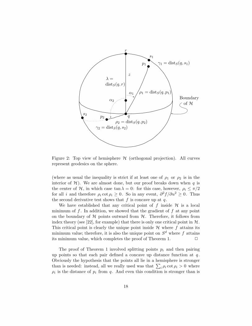
2(distS(s, p1))2 is concave up at s = q . For the induction step,let z be the geodesic which passes through both q and the center of thehemisphere H . For any point pi we define the angle αi to be the anglebetween z and the geodesic from q to pi , with the convention that αi = 0 ifpi lies on geodesic z in the direction from q to the center of the hemisphere(see Figure 2). First suppose there is some pi with αi = π/2. Then bychoice of z and since pi lies in the hemisphere H , the distance from q to pi

is ρi ≤ π/2 (or, if pi is the interior of H , then ρi < π/2). Thus cot ρi ≥ 0.We claim that this implies that the second derivative ∂2fi/∂u2 of fi isnon-negative (resp, positive if ρi < π/2). This claim follows immediatelyfrom the next lemma.

Lemma 4 Let α be the angle between the geodesic from q to pi and thegeodesic of u. Then ∂2fi/∂u2 = (sinα)2ρi cot ρi + (cos α)2.

Proof of Lemma: Let local axis v be the geodesic from q to pi and let y bea perpendicular local axis so that y makes angle π/2− α with u . Note theimages of v , t , y under the exponential map are coplanar. Lemma 2 impliesthat (∂2fi/∂v2)q = 1 and that (∂2fi/∂y2)q = ρi cot ρi . Using the chain rule,and differentiating twice,

∂fi

∂u=

∂fi

∂v

∂v

∂u+

∂fi

∂y

∂y

∂u=

∂fi

∂vcos α +

∂fi

∂ysinα.

∂2fi

∂u2=

∂2fi

∂v2cos2 α + 2

∂2fi

∂v∂ycos α sin α +

∂2fi

∂y2sin2 α.

By Lemma 2, the mixed partial is zero, so Lemma 4 is proved. 2

To complete the proof of Theorem 1, it remains to prove the inductionstep when there are no points which make angle π/2 with the geodesic z . ByTheorem 3, we know that the weighted sum of the vectors `q(pi)− q in thetangent hyperplane is equal to zero. Therefore, letting `q(z) be the imageof the axis z under the inverse exponential map, the sum of the projectionsof the vectors onto `q(z) is also zero; i.e.,∑n

i=1wiρi cos αi = 0. (5)

16

Since cosαi 6= 0 for all i , there are a pair of points, w.l.o.g. the points p1

and p2 , so that cosα1 > 0 and cosα2 < 0. Thus, 0 ≤ α1 < π/2 < α2 ≤ π .We shall prove by induction on n , the base case being n = 2, that when

(5) is satisfied for points in H , that ∂2f/∂u2 ≥ 0 (and > 0 if at leastone point lies in the interior of H). For the induction step, express f asf = f ′ + f ′′ as follows. Choose w′1 and w′2 so that 0 ≤ w′1 ≤ w1 and0 ≤ w′2 ≤ w2 and

w′1ρ1 cos α1 + w′2ρ2 cos α2 = 0

and so that either w′1 = w1 or w′2 = w2 . Define two functions f ′(x) =12(w′1distS(x, p1) + w′2distS(x, p2)) and f ′′(x) = f(x) − f ′(x). Since one ofthe first two coefficients in the formula for f ′′(x) is zero, f ′′(x) is a weightedsum of squares of distances of only n − 1 points from x . By construction,(5) holds for f ′′ , so the induction hypothesis applies to f ′′ . Similarly, f ′

satisfies (5) as a weighted sum of two points. Thus it will suffice to proveour claim for the n = 2 base case.

In the base case we have

w1ρ1 cos α1 + w2ρ2 cos α2 = 0. (6)

Since ρi cot ρi ≤ 1 and since cos2 αi + sin2 αi = 1, Lemma 4 implies that

∂2f/∂u2 ≥ w1ρ1 cot ρ1 + w2ρ2 cot ρ2 (7)

We define λ to equal the distance from q to the boundary of the hemi-sphere H , i.e., if the geodesic z from q to the center of H is extended pastthe center of H to the boundary of H at a point r , then λ is the geodesiclength from q to r . Likewise let s1 and s2 be the points on the boundaryof H which are reached by extending the geodesics from q through p1 and p2

and define γ1 and γ2 to be the distances from q to s1 and s2 , respectively.Consider the spherical right triangle with vertices q, r, s1 , which has a

right angle at r . The angle at vertex q is α1 , and a spherical right triangleidentity tells us that

cot γ1 tanλ = cos α1,

so therefore cot γ1 = (tanλ)−1 cos α1 . Since ρ1 ≤ γ1 and the cotangentfunction is deceasing for angles in the interval [0, π), we have

cot ρ1 ≥ (tanλ)−1 cos α1

with strict inequality if p1 is in the interior of H . This plus the correspondinginequality for cot ρ2 and equations (7) and (6) imply that

∂2f/∂u2 ≥ (tanλ)−1(w1ρ1 cos α1 + w2ρ2 cos α2) = 0

17

q

r

p1

s1

ρ1 = distS(q, p1)

γ1 = distS(q, s1)

Boundaryof H

p2s2

ρ2 = distS(q, p2)γ2 = distS(q, s2)

zλ =distS(q, r)

α1

α2

Figure 2: Top view of hemisphere H (orthogonal projection). All curvesrepresent geodesics on the sphere.

(where as usual the inequality is strict if at least one of ρ1 or ρ2 is in theinterior of H). We are almost done, but our proof breaks down when q isthe center of H , in which case tan λ = 0: for this case, however, ρi ≤ π/2for all i and therefore ρi cot ρi ≥ 0. So in any event, ∂2f/∂u2 ≥ 0. Thusthe second derivative test shows that f is concave up at q .

We have established that any critical point of f inside H is a localminimum of f . In addition, we showed that the gradient of f at any pointon the boundary of H points outward from H . Therefore, it follows fromindex theory (see [22], for example) that there is only one critical point in H .This critical point is clearly the unique point inside H where f attains itsminimum value; therefore, it is also the unique point on Sd where f attainsits minimum value, which completes the proof of Theorem 1. 2

The proof of Theorem 1 involved splitting points pi and then pairingup points so that each pair defined a concave up distance function at q .Obviously the hypothesis that the points all lie in a hemisphere is strongerthan is needed: instead, all we really used was that

∑i ρi cot ρi > 0 where

ρi is the distance of pi from q . And even this condition is stronger than is

18

really necessary except in the degenerate case where the points all lie in a(d− 1)-dimensional subspace of the sphere.

Thus there are various ways that the hypotheses of Theorem 1 can beweakened: two of these are stated in the next theorem. If q is a point on thesphere, then Bq(t) denotes the ball of radius t around q , namely, the set ofpoints on the sphere of distance ≤ t from q .

Theorem 5 Let f , pi , wi be as usual.(a) Let 0 < ϕ ≤ π/2. Suppose q is a critical point of f and Bq(ϕ) contains

points pi of total weight ≥ 0.5 and then all the points pi are contained inthe Bq(π − ϕ). Then q is a local minimum of f according to the secondderivative test.

(b) Let 0 < ϕ < ψ ≤ π/2. Suppose 0 < w ≤ 1 and that wϕ+(1−ψ)π ≤ ψ .Further suppose there is a point v so that Bv(ϕ) contains points pi oftotal weight ≥ w and that all the points pi are in Bv(π − 2ψ − ϕ). Thenf has a unique minimum. This unique minimum is inside Bv(ψ) and isthe only critical point inside Bv(ψ).

Proof Part (a) is immediate from the method used to prove Theorem 1:just match points outside of Bq(t) with points inside Bq(t).

To prove (b), note that the condition on w ensures that the globalminimum lies inside Bv(ψ). And any critical point inside Bv(ψ) satisfiesthe condition of part (a), with ϕ replaced by ϕ + ψ . 2

Part (b) of the theorem has the advantage that it is a test that can beapplied without having already found the critical point q . We conjecturethat part (b) can be substantially strengthened (see the final section).

2.2 Continuity of Spherical Weighted Averages

Theorem 6 Let values for p1, . . . , pn and w1, . . . , wn and q be chosen thatsatisfy the hypotheses of Theorem 1 or 5. Then there is a neighborhoodof p1, . . . , pn, w1, . . . , wn in which the weighted average q is a C∞ -functionof p1, . . . , pn, w1, . . . , wn .

This theorem is proved as a corollary of the Implicit Function Theorem(see Spivak [32]). Indeed, the weighted average q is equal to a root of ∇f .Except at points antipodal to one of the pi ’s, the function ∇f is clearlya C∞ -function of the points p1, . . . , pn and of the weights w1, . . . , wn .Furthermore, the matrix of first derivatives of ∇f is the Hessian matrix H .

19

Since the proof of Theorems 1 and 5 establishes that the second derivativetest shows that f is concave up, we know that the Hessian matrix His positive definite and thus non-singular. Therefore the conditions ofthe Implicit Function Theorem are satisfied at any point q satisfying theconditions of Theorems 1 or 5.

Note that the Inverse Function and Implicit Function Theorems can beused to calculate the first-order and higher-order derivatives of the weightedaverage function Avg .

It will be helpful in section 3 to know that the Hessian matrix His positive definite and non-singular in a neighborhood of the weightedaverage q . One further property: at every point q and every unit vector v ,we have vT Hv ≤ 1. This is proved by noting that lemma 2 shows that thisholds for the Hessians of the each of the Fi functions, since ρ cot ρ ≤ 1.

2.3 A Convexity Property

In this section we show that the points q which can be written as a weightedaverage of x1, . . . , xk form a convex set; in fact, they form precisely theconvex hull of the points x1, . . . , xk .

Definition A subset C of Sd is convex iff for any two points x, y ∈ C thereis a shortest geodesic from x to y which lies entirely in C .

The subset C is the convex hull of a set D iff C is the unique smallestconvex set containing D .

The above definition allows antipodal points to be in a convex set C , aslong as there is at least one geodesic between the antipodal points which liesin C . Note that if x1 and x2 are antipodal, then they do not have a convexhull. However, for any third point x3 , {x1, x2, x3} does have a convex hull,namely, the geodesic from x1 through x3 to x2 .

To state the next theorem with maximum generality, we define that apoint q is a proper weighted average of x1, . . . , xk if there are non-negativeweights w1, . . . , wk which sum to 1 such that q = ©

∑i wi · xi and there is a

hemisphere H such that for each non-zero wi , we have xi ∈ H , and that forat least one non-zero wi , xi is in the interior of H . The proper weightedaverages are of course precisely the weighted averages which are guaranteedby Theorem 1 to be uniquely defined. We say that the weighted average isstrongly proper provided the hemisphere H can be chosen so that each xi

with non-zero weight is in the interior of H .

20

Theorem 7 Suppose that x1, . . . , xk are distinct points, and that it notthe case that k = 2 with x1 and x2 antipodal. Then the convex hull Cof {x1, . . . , xk} exists and is equal to the set of proper weighted averagesof x1, . . . , xk . If x1, . . . , xk lie in a hemisphere, then the convex hull C is asubset of the hemisphere. If they do not lie in a hemisphere, then the convexhull is the entire sphere Sd .

Proof Let C be the intersection of all the hemispheres which contain{x1, . . . , xk} , or C = Sd if there are no such hemispheres. (Recall thathemispheres are always closed.) Clearly C is convex.

To show that every proper weighted average is in C , suppose that His a hemisphere containing all of x1, . . . , xk and that a point q is a properweighted average of x1, . . . , xk : we must show that q ∈ H . If some xi withnon-zero weight is in the interior of H , then Theorem 1 implies that q ∈ H .However, if every xi with non-zero weight is on the boundary of H , then itis obvious that q also lies on the boundary of H since q is a point where theweighted sum of squares of spherical distances is minimized. Hence q ∈ Hin either case.

It remains to to prove that every point q in C can be expressed as aproper weighted average of x1, . . . , xk . Since it is much simpler, we firstprove this in the special case where the points xi all lie in the interiorof a hemisphere H . Let x′i = `q(xi) be the point in the tangent plane Tq

corresponding to xi . The fact that q ∈ C implies that q is in the convex hullof the points x′i , since otherwise there is a closed halfplane G in Tq with qon its boundary which contains none of the points x′i , and its image expq(G)in Sd is a hemisphere which contains q but none of the xi ’s, contradictingthe fact that q ∈ C . Therefore q may be written as a Euclidean weightedaverage q =

∑i wix

′i , and now Theorems 1 and 3 imply that q is equal to

the proper, spherical weighted average q = ©∑

i wi · xi.Now we prove the more difficult general case. To handle the degenerate

cases, our proof proceeds by induction on the dimension d . For the basecase, d = 1, S1 is a circle. Let x1 and x2 be the first points clockwiseand counterclockwise (respectively) from q . Letting δ equal the sum of thearclengths from q to x1 and to x2 , it is clear that q ∈ C iff δ < π and thisholds iff q is a strongly proper weighted average of x1 and x2 .

Next we argue the induction step, d > 1. For r a point on Sd , let Hr

be the hemisphere centered at r . When q and xi are in Hr we define δr,xi

to be equal to the distance from xi to the boundary of Hr in the directionaway from q : i.e., measured along the geodesic containing q and xi . Weshall only consider points r which are in Hq , and letting δr,xi = 0 for xi not

21

in Hr , δr,xi is always defined for these r ’s. For each r ∈ Hq , define f(r) toequal the maximum value of δr,xi . Since f is a continuous function and hascompact domain, f attains a minimum value, f(s), at some point s ∈ Hq .

Let Ir denote the set of points xi which are in the interior of Hr . Firstsuppose that Is is non-empty or, equivalently, f(s) > 0. Let y1, . . . , y`

enumerate all the points xi which are in Is , and let zi = `q(yi) be thecorresponding points in the tangent plane Tq . We claim that q is in the(Euclidean) convex hull of {z1, . . . , z`} . To prove this claim, suppose it isfalse: then there is a vector ~v so that the dot product (zi − q) · ~v ≤ 0for all zi . Displace the point s infinitesimally in the direction ~v ; i.e., lets′ = expq(`q(s)+ε·~v) for sufficiently small ε > 0. Clearly, for small ε , we haveδs′,yi

< δs,yi for each yi ∈ Is . Also, for ε < f(s), we have δs′,x < ε < f(s) foreach x ∈ Is′ \ Is . Therefore, f(s′) < f(s) which contradicts the choice of s .That proves the claim that q is in the convex hull of {z1, . . . , z`} and thenexactly as argued in the preceding special case, Theorems 1 and 3 imply thatq is a (strongly) proper spherical weighted average of the points y1, . . . , y` .

Secondly, consider the case where Is = ∅ , so none of the points xi arein the interior of Hs . In this case, since q ∈ C , the point q must also lieon the boundary B of Hs (since the hemisphere with center antipodal to scontains all the points xi ). The boundary B is itself a (d − 1)-sphere. Itis easy to check that q is in every (d − 1)-hemisphere subset of B whichcontains every point xi ∈ B — this is because any such hemispheric subsetof B can be “lifted” to a hemispherical subset of Sd which contains everypoint xi . Therefore, by the induction hypothesis, q can be written as aproper weighted average of the points xi which lie in B . 2

The next theorem is a corollary to the method of proof of the previoustheorem,

Theorem 8 Suppose that x1, . . . , xk are distinct points, and that it not thecase that k = 2 with x1 and x2 antipodal. Then the convex hull C of{x1, . . . , xk} exists and is equal to the set of strongly proper weighted averagesof x1, . . . , xk .

In particular, q can be written as a proper weighted average of the points xi

if and only if it can be expressed as a strongly proper weighted average ofthe points. This can be further strengthened as follows:

Theorem 9 Every point in the convex hull C of {x1, . . . , xk} can be writtenas a strongly proper weighted average of at most d + 1 many of x1, . . . , xk .

Proof This follows from Theorems 8, 1 and 3 and corresponding fact forweighted averages in d-dimensional Euclidean spaces.

22

3 Algorithms for Spherical Weighted Averages

We now present two algorithms for computing a spherical weighted averageq = ©

∑ni=1 wi · pi . The first, Algorithm A1, is a linear convergence

rate algorithm which iteratively searches for a point q which satisfiesthe condition of Theorem 3. The second, Algorithm A2, is a quadraticconvergence rate algorithm which uses Newton descent to find a criticalpoint of the function f . Runtimes for these algorithms are reported insection 5.

Both algorithms are iterative, i.e., they start with an estimate for thevalue of q and produce a better estimate. To start the process, we choosean initial value q0 on the sphere taking the Euclidean weighted average ofthe points pi and normalizing to place on the sphere; namely,

q0 :=∑n

i=1 wipi / ||∑n

i=1 wipi||.If the hypotheses of Theorems 1 or 5 hold, then

∑i wipi is non-zero.

Given an estimate for q , Algorithm A1 maps all the points pi to thetangent hyperplane at q , then calculates their Euclidean weighted average uin the hyperplane and maps this back to the sphere by the exponential map.

Algorithm A1:Inputs: Points p1, . . . , pn on Sd

Non-negative weights w1, . . . , wn with sum 1.Output: The spherical weighted average of the inputs.Initialization: Set q :=

∑ni=1 wipi/||

∑ni=1 wipi|| .

Main Loop:For i = 1, . . . , n

Set p∗i := `q(pi)Set u :=

∑ni=1 wi(p∗i − q).

Set q := expq(q + u).If ||u|| is sufficiently small, output q and halt.Otherwise continue looping.

By Lemma 2 and the observation in the proof of Theorem 3, the vector uin the algorithm is the negative of the gradient ∇f(q) of f at q . Thus, theloop in Algorithm A1 is setting q = q −∇f , i.e., it moves q in the directionof steepest descent. We argue below that A1 converges linearly.

Next we give the Algorithm A2 which has a quadratic convergence rate.The main loop for Algorithm A2 updates an estimate q for the sphericalweighted average by computing the first-order and second-order derivatives

23

of the function f at the point q . It then inverts the Hessian matrix andcomputes a better estimate of the point where the first-derivative of f iszero.

Algorithm A2:Inputs: Points p1, . . . , pn on Sd

Non-negative weights w1, . . . , wn with sum 1.Output: The spherical weighted average of the inputs.Initialization: Set q :=

∑ni=1 wipi/||

∑ni=1 wipi|| .

Main Loop:Set up a local Euclidean coordinate system C at q .For i = 1, . . . , n

Set p∗i := `q(pi)Let ρi := ||p∗i − q|| .Set up a local coordinate system Ci at q such that the

first axis x(i)1 points in the direction away from pi .

Let Mi be the matrix that converts Ci coordinatesto C coordinates.

Let Hi be the d× d diagonal matrix with first entry 1and the rest of the entries ρi cot ρi .

Set u :=∑n

i=1 wi(p∗i − q).Set H :=

∑ni=1 MiHiM

Ti . (Note MT

i = M−1i , the transpose of M )

Set v := H−1u .Set q := expq(q + v).If ||v|| is sufficiently small, output q and halt.Otherwise continue looping.

By Lemma 2, each Hi is the Hessian matrix of fi at the point q inthe coordinate system Ci ; and H is the Hessian matrix of f at q in thecoordinate system C . The points p∗ and the negative gradient u are to berepresented in the coordinate system C . To see that the convergence rate ofAlgorithm A2 is really quadratic, note that it is performs Newton’s algorithmfor finding a root of ∇f ; namely it updates q by q = q −H(∇f). As notedafter Theorem 6, the Hessian H is positive definite in a neighborhood ofthe weighted average qsoln . In addition, by finite dimensionality, u · Huis bounded away from zero in a neighborhood of qsoln . These facts aresufficient for Newton’s algorithm to converge quadratically, see e.g. Theorem1.4.6 of Polak [26].

We have u = Hv , so by comments after Theorem 6, 1 ≥ v · u > ε for

24

some ε > 0 in some neighborhood of qsoln . From this it can be shown, againin a sufficiently small neighborhood of qsoln , that if q′ = expq(q + u), thenf(q′) < δf(q) for some 0 < δ < 1. This implies that A1 converges at leastlinearly.

The above discussion on convergence rates only covers local convergence,i.e., convergence assuming that q is already sufficiently close to qsoln . Itis possible to convert these algorithms into ones with guaranteed globalconvergence (c.f. [26]), but in practice we have never seen a situation whereAlgorithms A1 and A2 failed to converge well.

4 Applications to Splines

4.1 Splines Based on Weighted Spherical Averages

Spline curves are curves which are specified by a small set of parametersand which have nice smoothness properties, such as having continuous k -thorder derivatives. They are widely used in drafting and computer aidedmanufacturing to specify curves and surfaces. In robotics and animation,spherical splines are often used to specify orientations for smooth kinematicmotion of solid bodies.

We consider the problem of specifying spline functions which take valueson the unit d-sphere Sd : these are useful for a variety of applications.In graphics and robotics, the most prominent applications are based onthe equivalence between quaternions and (pairs of antipodal) points on the3-sphere. A spline function taking values on the 3-sphere can be used as aspline function taking quaternion values and, if the curve is parameterizedby time t , then the spline curve specifies the orientation of a solid body asa smooth function of time.

The most common method of using splines in Euclidean space Rd+1

involves the selection of control points p1, . . . , pn in Rd+1 and blendingfunctions f1(t), . . . , fn(t), also called basis functions. The Euclidean splinecurve s(t) is defined by

s(t) =∑n

i=1fi(t)pi.

The blending functions must always satisfy the properties

f1(t) + f2(t) + · · ·+ fn(t) = 1 and fi(t) ≥ 0, for all i , (8)

for t in the interval [a, b] . Usually the blending functions enjoy additionalproperties such as having continuous k -th order derivatives; or being

25

‘bitonic’, i.e., being increasing on an initial part of the interval [a, b] anddecreasing on the the rest of the interval; or having local support.

In order to define spherical splines, let p1, . . . , pn now be points on Sd ,and let f1(t), . . . , fn(t) be functions which satisfy (8). We define a splinecurve s(t) which takes values on the unit sphere by setting

s(t) = ©∑n

i=1fi(t) · pi.

In practice, we should ensure that for each value of the parameter t , the setof control points pi for which fi(t) 6= 0 is contained inside a hemisphere, orat least is mostly contained inside a hemisphere so as to satisfy the conditionsof Theorems 1 or 5. This condition is most readily met provided that either(a) the blending functions have local support and consecutive control pointsare not too widely spaced, or (b) the control points all lie inside a singlehemisphere.

The most common applications of splines use B-splines with theblending functions fi being piecewise cubic curves with continuous sec-ond derivatives. To define the B-spline curves, one picks control pointsa = t1, t2, . . . , tn−1, tn = b (to be precise, one may also pick additionalcontrol points, but this does not impact the present discussion), which thendetermine the blending functions. The blending functions have the propertythat for tj ≤ t ≤ tj+1 , the only non-zero fi(t) are for i ∈ {j−1, j, j+1, j+2} .In particular, fi(tj) is non-zero only if i ∈ {j − 1, j, j + 1} . In this casethe spherical spline points s(t) will be well-defined provided that any fourconsecutive control points lie in a hemisphere. Of course, this requirementthat any four consecutive control points lie in a hemisphere can be relaxedsomewhat, in light of Theorem 5.

Theorem 6 implies that if the the blending functions fi have continuousk -th derivatives, then the spline curve s(t) also has continuous k -thderivatives.

Since Bezier curves are special cases of B-spline curves, one can definespherical Bezier curves in terms of our B-spline curves. These curveswill generally be different than the spherical Bezier curves generated byde Casteljau methods.

4.2 Interpolation with Spherical Splines

The previous discussion concerned B-spline curves defined with controlpoints — in general, the curve does not pass through the control points.We now take up the problem of defining a spline curve that interpolates adesired set of points.

26

Suppose we are given points c1, . . . , cn on the d-sphere, and are giventime values t1 < t2 < · · · < tn : we wish to find a smooth curve s lyingon the sphere, parameterized by t , so that s(t1) = ci for all i . The basicproblem is to choose additional knot positions and control points pi whichdefines a spherical spline curve which satisfies these conditions.

There are of course a variety of possible ways to define B-spline curves:for experimental purposes, we have implemented one kind of B-spline curvethat gives blending functions which are piecewise cubic polynomials andwhich have continuous second derivatives. We implemented two sets ofalgorithms, one with a linear convergence rate and one with a quadraticconvergence rate, for both the 2-sphere and the 3-sphere. We report timingresults below, but since the linear convergence rate algorithm worked almostas fast as the quadratic convergence rate algorithm, and since the formeralgorithm is much easier to describe and to implement, we will describe onlythe first algorithm in detail.

We used a standard B-spline implementation (see, e.g., [38]) having asknot positions the values t0, t1, t2, . . . , tn+4, tn+5 with t0 = t1 = t2 = t3 andtn+5 = tn+4 = tn+3 = tn+2 . We ‘double’ the first and last control points,requiring that p0 = p1 and pn+1 = pn . Our blending functions are definedas usual for piecewise-cubic B-splines, namely, define

Bi,1(t) =

{1 if ti ≤ t < ti+1

0 otherwise

andBi,n+1(t) =

t− titi+n − ti

Bi,n(t) +ti+n+1 − t

ti+n+1 − ti+1Bi+1,n(t),

using the convention that 0/0 = 0. The blending functions are defined byfi(t) = Bi,4(t), are defined for t ∈ [t3, tn+2] , are piecewise cubic, and havecontinuous second derivatives. The support of fi is in the interval [ti, ti+4] .The spline curve is given by s(t) = ©

∑n+1i=0 fi(t) · pi .

Once we have the blending functions, it remains to choose controlpoints pi so that the points ci are interpolated correctly, with s(ti+1) = ci .In the Euclidean setting, this yields a set of linear equalities given by a

27

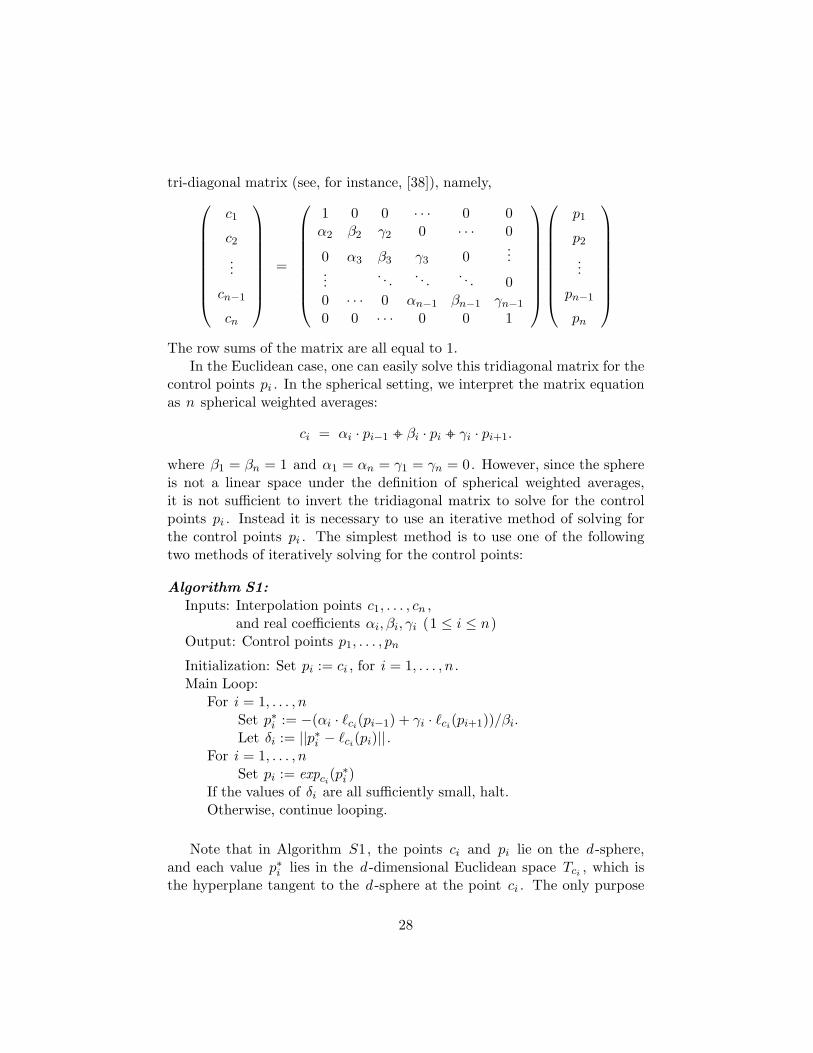
tri-diagonal matrix (see, for instance, [38]), namely,

c1

c2

...

cn−1

cn

=

1 0 0 · · · 0 0α2 β2 γ2 0 · · · 0

0 α3 β3 γ3 0...

.... . . . . . . . . 0

0 · · · 0 αn−1 βn−1 γn−1

0 0 · · · 0 0 1

p1

p2

...

pn−1

pn

The row sums of the matrix are all equal to 1.In the Euclidean case, one can easily solve this tridiagonal matrix for the

control points pi . In the spherical setting, we interpret the matrix equationas n spherical weighted averages:

ci = αi · pi−1 ◦+ βi · pi ◦+ γi · pi+1.

where β1 = βn = 1 and α1 = αn = γ1 = γn = 0. However, since the sphereis not a linear space under the definition of spherical weighted averages,it is not sufficient to invert the tridiagonal matrix to solve for the controlpoints pi . Instead it is necessary to use an iterative method of solving forthe control points pi . The simplest method is to use one of the followingtwo methods of iteratively solving for the control points:

Algorithm S1:Inputs: Interpolation points c1, . . . , cn ,

and real coefficients αi, βi, γi (1 ≤ i ≤ n)Output: Control points p1, . . . , pn

Initialization: Set pi := ci , for i = 1, . . . , n .Main Loop:

For i = 1, . . . , nSet p∗i := −(αi · `ci(pi−1) + γi · `ci(pi+1))/βi.Let δi := ||p∗i − `ci(pi)|| .

For i = 1, . . . , nSet pi := expci

(p∗i )If the values of δi are all sufficiently small, halt.Otherwise, continue looping.

Note that in Algorithm S1, the points ci and pi lie on the d-sphere,and each value p∗i lies in the d-dimensional Euclidean space Tci , which isthe hyperplane tangent to the d-sphere at the point ci . The only purpose

28

of computing the scalar values δi is to measure the distance between theold and new values of pi , so as to have a stopping criterion. The generalidea behind the algorithm is quite simple: the new value of pi is set so thatits weighted average with the old values of pi−1 and pi+1 would correctlygive the interpolation point ci . Of course, since all the pi values are beingupdated at once, a single iteration of the loop does not yield a solution. Butsince the diagonal entries of the matrix dominate the off-diagonal entries,the iteration converges towards a solution.

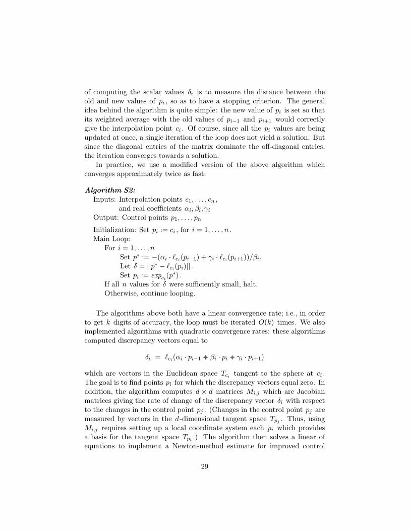
In practice, we use a modified version of the above algorithm whichconverges approximately twice as fast:

Algorithm S2:Inputs: Interpolation points c1, . . . , cn ,

and real coefficients αi, βi, γi

Output: Control points p1, . . . , pn

Initialization: Set pi := ci , for i = 1, . . . , n .Main Loop:

For i = 1, . . . , nSet p∗ := −(αi · `ci(pi−1) + γi · `ci(pi+1))/βi.Let δ = ||p∗ − `ci(pi)|| .Set pi := expci

(p∗).If all n values for δ were sufficiently small, halt.Otherwise, continue looping.

The algorithms above both have a linear convergence rate; i.e., in orderto get k digits of accuracy, the loop must be iterated O(k) times. We alsoimplemented algorithms with quadratic convergence rates: these algorithmscomputed discrepancy vectors equal to

δi = `ci(αi · pi−1 ◦+ βi · pi ◦+ γi · pi+1)

which are vectors in the Euclidean space Tci tangent to the sphere at ci .The goal is to find points pi for which the discrepancy vectors equal zero. Inaddition, the algorithm computes d × d matrices Mi,j which are Jacobianmatrices giving the rate of change of the discrepancy vector δi with respectto the changes in the control point pj . (Changes in the control point pj aremeasured by vectors in the d-dimensional tangent space Tpj . Thus, usingMi,j requires setting up a local coordinate system each pi which providesa basis for the tangent space Tpi .) The algorithm then solves a linear ofequations to implement a Newton-method estimate for improved control

29

points.The disadvantage of the quadratic convergence rate method is that it is

much more difficult to implement than Algorithms S1 or S2. Furthermorethe runtime is not greatly improved over the linear convergence ratealgorithms, since each loop iteration is much slower. We tested the runtimesof the various algorithms to obtain approximately 16 digits of accuracy (theIEEE floating point double precision limits). When d = 2 (for finding splineson the 2-sphere embedded in R3 ), the quadratic convergence rate methodwas experimentally observed to be twice the speed of the linear convergencerate method. However, for d = 3 (for splines on S3 or for quaternion splinecurves), the quadratic convergence rate method was slightly slower than thelinear convergence rate algorithm.

In view of the relatively lackluster performance advantage of thequadratic convergence rate algorithm, and in view of the substantial difficultyof implementing the quadratic convergence rate methods, we recommend useof the linear convergence rate methods only.

4.3 Examples of Spline Interpolation

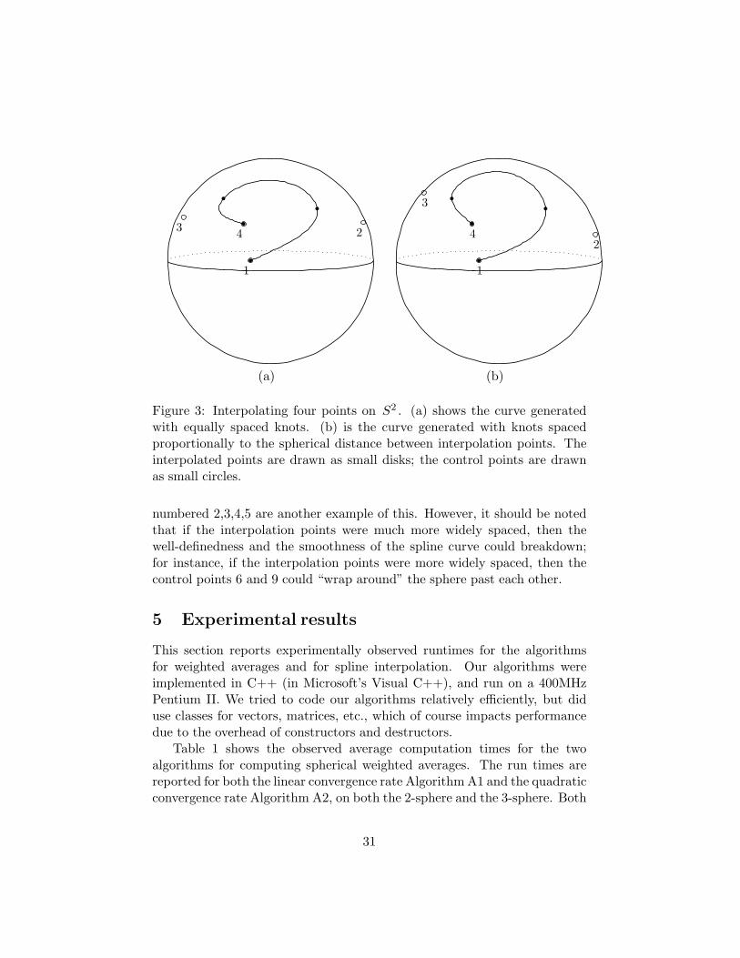
Figures 3 and 4 show some experimental results of spline interpolation.Figures 3a and 3b show curves which interpolate four points on the sphere— the control points for the curve are shown as open circles and are seen tolie completely within one hemisphere. For Figure 3a, the knots were equallyspaced; and for Figure 3b, the knots were spaced proportionally to sphericaldistance between the interpolation points. Clearly the second version withunequally spaced knots yields a more rounded, smoothly varying curve. Itis beyond the scope of the present paper to investigate the best methodsof choosing knot positions; rather, we are using this as an example of howtechniques for generating Euclidean spline curves can now be applied tocurves on spheres.

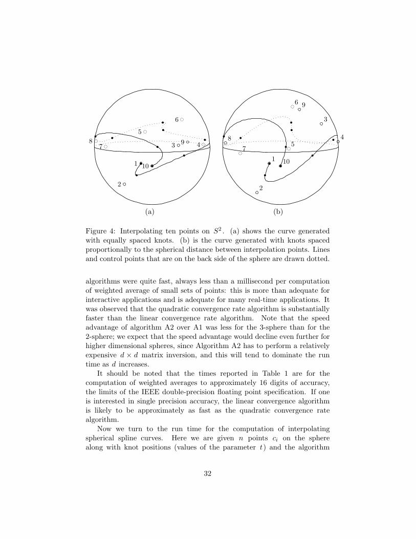
Figure 4 shows curves that interpolate 10 points that circumnavigate the2-sphere. Again, Figure 4a shows the result of choosing equally spaced knotsand Figure 4b shows the curve obtained with knots spaced proportionallyto the spherical distance between the interpolation points. Once again,the use of unequally spaced knots yields a smoother looking curve. Oneinteresting feature of the control points shown in the curves Figure 4 is thatthey do not satisfy the hypotheses of Theorem 1. For example, the controlpoints numbered 6,7,8,9 in Figure 4a do not lie in a single hemisphere:nonetheless, the spherical distance is still well-defined for the points on thespline curve and the spline curve still varies smoothly. The control points

30

1

23 4

1

2

3

4

(a) (b)

Figure 3: Interpolating four points on S2 . (a) shows the curve generatedwith equally spaced knots. (b) is the curve generated with knots spacedproportionally to the spherical distance between interpolation points. Theinterpolated points are drawn as small disks; the control points are drawnas small circles.

numbered 2,3,4,5 are another example of this. However, it should be notedthat if the interpolation points were much more widely spaced, then thewell-definedness and the smoothness of the spline curve could breakdown;for instance, if the interpolation points were more widely spaced, then thecontrol points 6 and 9 could “wrap around” the sphere past each other.

5 Experimental results

This section reports experimentally observed runtimes for the algorithmsfor weighted averages and for spline interpolation. Our algorithms wereimplemented in C++ (in Microsoft’s Visual C++), and run on a 400MHzPentium II. We tried to code our algorithms relatively efficiently, but diduse classes for vectors, matrices, etc., which of course impacts performancedue to the overhead of constructors and destructors.

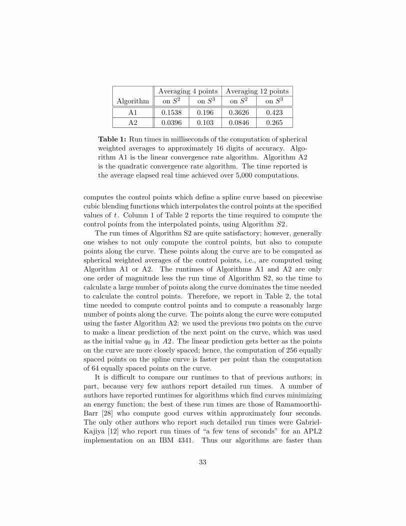
Table 1 shows the observed average computation times for the twoalgorithms for computing spherical weighted averages. The run times arereported for both the linear convergence rate Algorithm A1 and the quadraticconvergence rate Algorithm A2, on both the 2-sphere and the 3-sphere. Both

31

1

2

3 4

5

6

78 9

101

2

3

45

6

7

8

9

10

(a) (b)

Figure 4: Interpolating ten points on S2 . (a) shows the curve generatedwith equally spaced knots. (b) is the curve generated with knots spacedproportionally to the spherical distance between interpolation points. Linesand control points that are on the back side of the sphere are drawn dotted.

algorithms were quite fast, always less than a millisecond per computationof weighted average of small sets of points: this is more than adequate forinteractive applications and is adequate for many real-time applications. Itwas observed that the quadratic convergence rate algorithm is substantiallyfaster than the linear convergence rate algorithm. Note that the speedadvantage of algorithm A2 over A1 was less for the 3-sphere than for the2-sphere; we expect that the speed advantage would decline even further forhigher dimensional spheres, since Algorithm A2 has to perform a relativelyexpensive d × d matrix inversion, and this will tend to dominate the runtime as d increases.

It should be noted that the times reported in Table 1 are for thecomputation of weighted averages to approximately 16 digits of accuracy,the limits of the IEEE double-precision floating point specification. If oneis interested in single precision accuracy, the linear convergence algorithmis likely to be approximately as fast as the quadratic convergence ratealgorithm.

Now we turn to the run time for the computation of interpolatingspherical spline curves. Here we are given n points ci on the spherealong with knot positions (values of the parameter t) and the algorithm

32

Averaging 4 points Averaging 12 pointsAlgorithm on S2 on S3 on S2 on S3

A1 0.1538 0.196 0.3626 0.423A2 0.0396 0.103 0.0846 0.265

Table 1: Run times in milliseconds of the computation of sphericalweighted averages to approximately 16 digits of accuracy. Algo-rithm A1 is the linear convergence rate algorithm. Algorithm A2is the quadratic convergence rate algorithm. The time reported isthe average elapsed real time achieved over 5,000 computations.

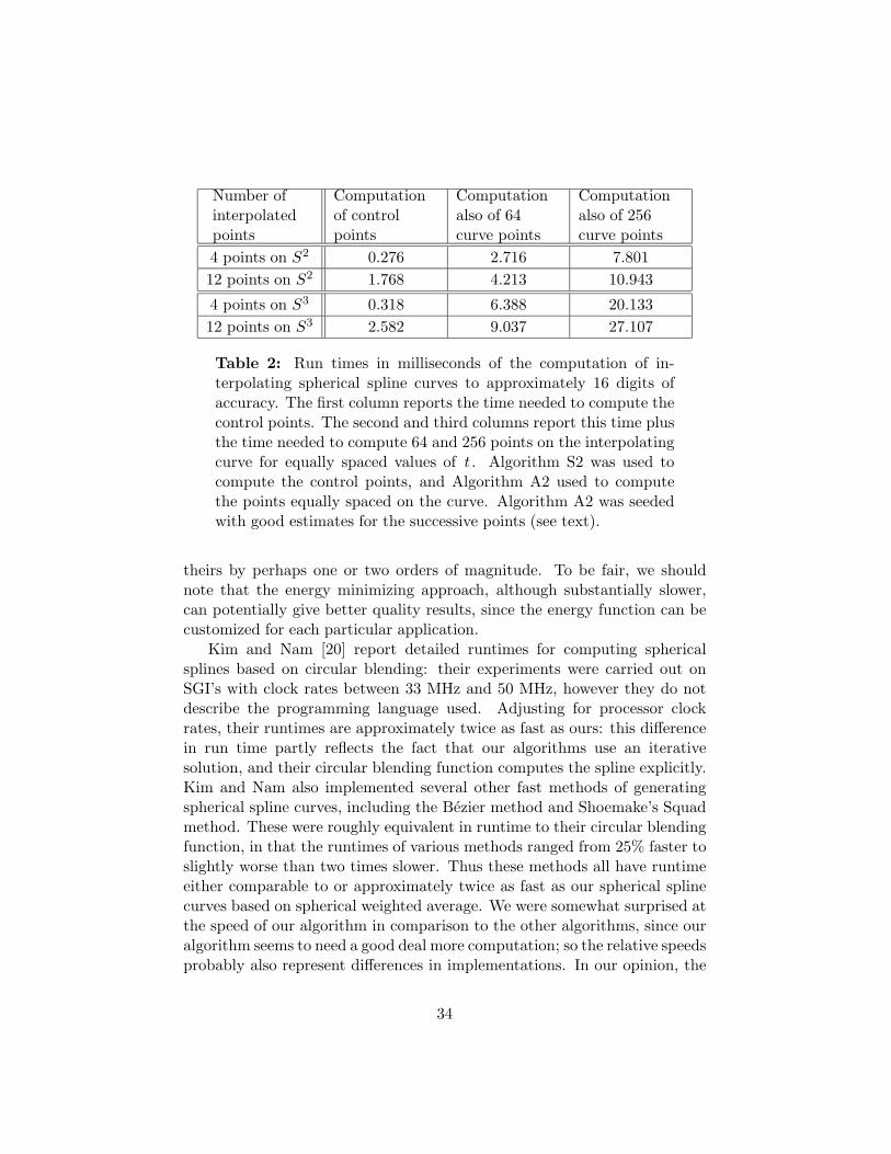
computes the control points which define a spline curve based on piecewisecubic blending functions which interpolates the control points at the specifiedvalues of t . Column 1 of Table 2 reports the time required to compute thecontrol points from the interpolated points, using Algorithm S2.

The run times of Algorithm S2 are quite satisfactory; however, generallyone wishes to not only compute the control points, but also to computepoints along the curve. These points along the curve are to be computed asspherical weighted averages of the control points, i.e., are computed usingAlgorithm A1 or A2. The runtimes of Algorithms A1 and A2 are onlyone order of magnitude less the run time of Algorithm S2, so the time tocalculate a large number of points along the curve dominates the time neededto calculate the control points. Therefore, we report in Table 2, the totaltime needed to compute control points and to compute a reasonably largenumber of points along the curve. The points along the curve were computedusing the faster Algorithm A2: we used the previous two points on the curveto make a linear prediction of the next point on the curve, which was usedas the initial value q0 in A2. The linear prediction gets better as the pointson the curve are more closely spaced; hence, the computation of 256 equallyspaced points on the spline curve is faster per point than the computationof 64 equally spaced points on the curve.

It is difficult to compare our runtimes to that of previous authors; inpart, because very few authors report detailed run times. A number ofauthors have reported runtimes for algorithms which find curves minimizingan energy function; the best of these run times are those of Ramamoorthi-Barr [28] who compute good curves within approximately four seconds.The only other authors who report such detailed run times were Gabriel-Kajiya [12] who report run times of “a few tens of seconds” for an APL2implementation on an IBM 4341. Thus our algorithms are faster than

33

Number ofinterpolatedpoints

Computationof controlpoints

Computationalso of 64curve points

Computationalso of 256curve points

4 points on S2 0.276 2.716 7.80112 points on S2 1.768 4.213 10.943

4 points on S3 0.318 6.388 20.13312 points on S3 2.582 9.037 27.107

Table 2: Run times in milliseconds of the computation of in-terpolating spherical spline curves to approximately 16 digits ofaccuracy. The first column reports the time needed to compute thecontrol points. The second and third columns report this time plusthe time needed to compute 64 and 256 points on the interpolatingcurve for equally spaced values of t . Algorithm S2 was used tocompute the control points, and Algorithm A2 used to computethe points equally spaced on the curve. Algorithm A2 was seededwith good estimates for the successive points (see text).

theirs by perhaps one or two orders of magnitude. To be fair, we shouldnote that the energy minimizing approach, although substantially slower,can potentially give better quality results, since the energy function can becustomized for each particular application.

Kim and Nam [20] report detailed runtimes for computing sphericalsplines based on circular blending: their experiments were carried out onSGI’s with clock rates between 33 MHz and 50 MHz, however they do notdescribe the programming language used. Adjusting for processor clockrates, their runtimes are approximately twice as fast as ours: this differencein run time partly reflects the fact that our algorithms use an iterativesolution, and their circular blending function computes the spline explicitly.Kim and Nam also implemented several other fast methods of generatingspherical spline curves, including the Bezier method and Shoemake’s Squadmethod. These were roughly equivalent in runtime to their circular blendingfunction, in that the runtimes of various methods ranged from 25% faster toslightly worse than two times slower. Thus these methods all have runtimeeither comparable to or approximately twice as fast as our spherical splinecurves based on spherical weighted average. We were somewhat surprised atthe speed of our algorithm in comparison to the other algorithms, since ouralgorithm seems to need a good deal more computation; so the relative speedsprobably also represent differences in implementations. In our opinion, the

34

advantages of our splines as outlined in the introduction outweigh theirslower computation time in many potential applications; and in any event,our spherical spline curve algorithms are sufficiently fast for all but the mosttime critical applications.

6 Open Problems

We conclude with a few remarks about open problems and the possibilityof improving the analysis and applications of our spherical spline curves infuture work.

First, we have not yet derived formulas for computing the covariantderivatives of our spherical spline curves. In particular, the proof ofTheorem 6 based on the Implicit Function theorem should yield formulasfor the derivatives of the function ©

∑i wi · pi with respect to changes in

the values of wi and of pi . Given formulas for the first- and second-orderderivatives of the spline curve, it should be possible to use iterative methodsfor finding control points that define “natural splines” which minimize thecurvature or the second derivatives of the spline curve. Likewise, we expectthat one could minimize energy functions, etc.

Second, it would be useful to extend methods of knot insertion fromthe Euclidean domain to the spherical domain. In the Euclidean domain,knot insertion is a technique that allows the insertion of additional knotsand control points without altering the spline curve. This is useful forseveral purposes including efficiently rendering curves to any desired level ofdetail and for optimizing trajectories specified with splines (see, e.g., [27] forthe latter application). The standard knot insertion algorithms all dependstrongly on the linearity of Euclidean space, so they are not immediatelyapplicable to spherical spline curves based on spherical weighted averages. Itis plausible that techniques similar to those of Brown and Worsey [5] couldbe used to prove that knot insertion is not possible on the sphere.

Third, it would be nice to prove stronger forms of Theorem 5, particularlyforms that would be more useful for spline curves by relaxing the conditionthat any four successive control points lie in a hemisphere. For instance, weconjecture that if each pair of successive control points of a B-spline curveare separated by a distance of no more than π/2, then the spherical weightedaverages in the definition of the spline curve are always uniquely defined andare local minima according to the second derivative test.

Fourth, there is another, yet unexplored alternative to defining sphericalaverages, based on the characterization of barycentric coordinates in terms

35

of areas of triangles (or in higher dimensions, simplices). This could beused to give an alternate definition of spherical averages, and it wouldbe interesting to understand how this is related to the spherical averagesof the present paper: it is not hard to give examples where they differ.We have not pursued since alternative for two reason: first, the area-baseddefinition would seemingly only allow averages of d+1 points in the d-sphereand, second, since the definition based on minimization of square distanceseemed more compelling and elegant. Along these lines, there may besome connection Arvo’s algorithm [2] for area-uniform sampling of sphericaltriangles.

Fifth, and perhaps most interesting, it would be desirable to extend thespherical averages to more general manifolds. The definition of an average asthe point which minimizes the weighted sum of the squares of the distancesfrom the pi ’s could apply to any manifold (or subset of a manifold) in which,for any two given points, there is a shortest geodesic joining the points. Itwould be nice to have general conditions on manifolds, or the distributionof points pi on the manifold, which imply that the weighted average iswell-defined in this way. Ideally, this would allow the notion of weightedaverages to be extended to a broad range of manifolds.

Acknowledgements We thank B. Ravani for comments on a draft ofthe paper, and especially for the suggestion that we prove convexityproperties. The first author thanks S. Rotenberg for useful discussions,and for introducing him to slerping. Finally, we thank the referees for usefulsuggestions.

References

[1] P. Alfeld, M. Neamtu, and L. L. Shumaker, Bernstein-Bezier polyno-mials on spheres and sphere-like surfaces, Computer Aided Geometric Design,13 (1996), pp. 333–349.

[2] J. Arvo, Startified sampling of spherical triangles, Computer Graphics, 29(1995), pp. 437–438. SIGGRAPH ’95.

[3] M. Baronti, E. Casini, and P. L. Papini, Centroids, centers and medians:What is the difference?, Geometriae Dedicata, 68 (1997), pp. 157–168.

[4] A. H. Barr, B. Currin, S. Gabriel, and J. Hughes, Smooth interpolationof orientations with angular velocity constraints using quaternions, in Com-puter Graphics: SIGGRAPH’92 Conference Proceedings, 1992, pp. 313–320.

[5] J. L. Brown and A. J. Worsey, Problems with defining barycentriccoordinates for the sphere, Mathematical Modelling and Numerical Analysis(Modelisation mathematique et Analyse numerique), 26 (1992), pp. 37–49.

36

[6] R. M. Clark and R. Thompson, Statistical comparison of palaeomagneticdirectional records from lake sediment, Geophys. J. R. Astr. Soc., 76 (1984),pp. 337–368.

[7] H. S. M. Coxeter, Quaternions and reflections, American MathematicalMonthly, 53 (1946), pp. 136–146.

[8] E. B. Dam, M. Koch, and M. Lillholm, Quaternions, interpolation andanimation, Tech. Rep. DIKU 98/5, Institute of Computer Science, Univ. ofCopenhagen, 1998. http://www.diku.dk/students/myth/quat.html.

[9] T. Duff, Splines in animation and modeling, in SIGGRAPH’86 Course Noteson State of the Art in Image Synthesis, ACM, July 1986.

[10] G. Farin, Curves and Surfaces for Computer Aided Geometric Design: APractical Guide, Academic Press, Boston, 3rd ed., 1993. Contains chapters byP. Bezier and W. Boehm.

[11] N. I. Fisher and T. Lewis, A note on spherical splines, J. R. Statist. Soc.B, 47 (1985), pp. 482–488.

[12] S. Gabriel and K. Kajiya, Spline interpolation in curved space, inSIGGRAPH’85 Course Notes on State of the Art Image Synthesis, ACM,1985, pp. 1–14.

[13] Q. J. Ge and B. Ravani, Computer aided geometric design of motioninterpolants, Transactions of the ASME: Journal of Mechanical Design, (1994),pp. 756–762. Earlier version in Adv. in Design Automation, ASME, DE-Vol32-2, 1991, pp.33-41.

[14] O. Gross, The rondezvous value of a metric space, in Advances in GameTheory, Princeton University Press, 1964, pp. 49–53.

[15] J. C. Hart, G. K. Francis, and L. H. Kauffman, Visualizing quaternionrotation, ACM Transactions on Graphics, 13 (1994), pp. 256–276.

[16] P. E. Jupp, Fitting smooth paths to spherical data, Applied Statistics, 36(1987), pp. 34–46.

[17] B. Juttler, Visualization of moving objects using dual quaternion curves,Comput. and Graphics, 18 (1994), pp. 315–326.

[18] B. Juttler and M. G. Wagner, Computer-aided design with spatial rationalB-spline motions, Journal of Mechanical Design, 118 (1996), pp. 193–201.

[19] M.-J. Kim, M.-S. Kim, and S. Y. Shin, A general construction schemefor unit quaternion curves with simple high order derivatives, in ComputerGraphics: SIGGRAPH’95 Conference Proceedings, 1985, pp. 369–376.

[20] M.-S. Kim and K.-W. Nam, Interpolating solid orientations with circularblending quaternion curves, Computer Aided Design, 27 (1995), pp. 385–398.

[21] , Hermite interpolation of solid orientations with circular blendingquaternion curves, Journal of Visualization and Computer Animation, 7(1996), pp. 95–110.

37

[22] J. W. Milnor, Topology from the Differentiable Viewpoint, University Pressof Virginia, Charlottesville, 1965. Based on notes by D.W. Weaver.

[23] L. Noakes, G. Heinzinger, and B. Paden, Cubic splines on curved surfaces,IMA Journal of Mathematical Control and Information, 6 (1989), pp. 465–473.

[24] F. C. Park and B. Ravani, Smooth invariant interpolation of rotations,ACM Transactions on Graphics, 16 (1997), pp. 227–295.

[25] R. L. Parker and C. F. Denham, Interpolation of unit vectors, GeophysicalJournal of the Royal Astronomical Society, 58 (1979), pp. 685–687.

[26] E. Polak, Optimization: Algorithms and Consistent Approximations, AppliedMathematical Sciences #124, Springer-Verlag, New York, 1997.

[27] R. Ramamoorthi, C. Ball, and A. H. Barr, Dynamic splines withconstraints for animation, Tech. Rep. CS-TR-97-03, Dept. of ComputerScience, CalTech, 1997.

[28] R. Ramamoorthi and A. H. Barr, Fast constuction of quaternion splines, inComputer Graphics: SIGGRAPH’97 Conference Proceedings, 1997, pp. 287–292.

[29] K. S. Roberts, G. Bishop, and S. K. Ganapathy, Smooth interpolation ofrotational matrices, in Proceedings CVPR’88: Computer Vision and PatternRecognition, IEEE Computer Science Press, 1988, pp. 724–729.

[30] K. Shoemake, Animating rotation with quaternion curves, Computer Graph-ics, 19 (1985), pp. 245–254. SIGGRAPH’85.

[31] , Quaternion calculus and fast animation, in SIGGRAPH’87 CourseNotes on State of the Art Image Synthesis, ACM, 1987, pp. 101–121.

[32] M. Spivak, Calculus on Manifolds, Benjamin/Cummings Publishing, MenloPark, 1965.

[33] R. Thompson and R. M. Clark, A robust least-squares Gondwanan apparentpolar wander path and the question of paleomagnetic assessment of Gondwananreconstructions, Earth and Planetary Science Letters, 57 (1982), pp. 152–158.

[34] G. Wagner, On means of distances on the surface of a sphere (lower bounds),Pacific Journal of Mathematics, 144 (1990), pp. 389–398.

[35] , On means of distances on the surface of a sphere. II (lower bounds),Pacific Journal of Mathematics, 154 (1992), pp. 381–396.

[36] W. Wang and B. Joe, Orientation interpolation in quaternion space usingspherical biarcs, in Graphics Interface’93, 1993, pp. 24–32.

[37] G. S. Watson, Statistics on Spheres, J. Wiley & Sons, New York, 1983.

[38] A. Watt and M. Watt, Advanced Animation and Rendering Techniques,Addison-Wesley, Reading, Massachusetts, 1992.

[39] R. Wolf, On the average distance property of spheres in Banach spaces,Archives of Mathematics, 62 (1994), pp. 338–344.

38

[40] M. Zefran and V. Kumar, Planning of smooth motions on SE(3), in Proc.IEEE International Conference on Robotics and Animation, IEEE, 1996,pp. 121–126.

39