Speculative Attacks and Financial Architecture:

Experimental Analysis of Coordination Games

with Public and Private Information*

Frank Heinemanna, Rosemarie Nagelb and Peter Ockenfelsc

First version 7. August 2001. This version 17.6.2002

Abstract

Speculative Attacks can be modeled as a coordination game with multiple equilibria if the state of the economy is common knowledge. With private information there is a unique equilibrium. This raises the question whether public information may be destabilizing by allowing for self-fulfilling beliefs. We present an experiment that imitates a speculative attacks model and compare sessions with public and private information. In both treatments subjects use so-called threshold strategies that lie in between the risk dominant and payoff dominant equilibrium of the underlying complete information game. Our evidence suggests that there are no destabilizing effects due to public information. In contrary, predictability of attacks is slightly higher with public than with private information, but prior probability of attacks is also higher with public information. We also test the predictive power of refinement theories to explain actual behavior and reactions to parameter changes.

Keywords: Coordination game, global game, payoff dominance, private information, public information, risk dominance, strategic uncertainty, supermodular game.

JEL codes: C72, C 91, E 58.

* We want to thank Werner Güth, Stephen Morris and Hyun Shin for stimulating comments, Dörte Dömeland, Isabel Gödde and various colleges at Goethe-Universität Frankfurt for helpful discussions on statistical procedures and tests. All errors remain our own responsibility. We are indebted to Urs Fischbacher for his fabulous software package z-Tree that we used for our experiments and to Martin Menner for helping to organize the sessions in Barcelona. Finally, we thank students at Goethe-Universität Frankfurt and Universitat Pompeu Fabra in Barcelona for their participation in our experiments. Financial support by the Volkswagen Foundation and the Landeszentralbank Hessen is gratefully acknowledged. Frank Heinemann acknowledges financial support by the TMR network on “Financial Market Efficiency and Economic Efficiency”. Rosemarie Nagel acknowledges financial support of Spain’s Ministry of Education under grant PB98-1076. a Ludwig-Maximilians-Universität München. b Universitat Pompeu Fabra, Barcelona. c Goethe-Universität Frankfurt am Main.

1

1. Introduction

Transparency and the optimal way to disclose central bank information are among the main topics within the current discussion on financial architecture. Speculative attacks and market overreactions are often interpreted as evidence for systemic indeterminacy and instability. Recent theories attribute these instabilities to self-fulfilling beliefs caused by public information and suggest that stability can be increased by more sophisticated schemes of information disclosure. In this paper we present an experiment designed to test these theories.

Obstfeld (1996) models speculative attacks as a coordination game with strategic complementarities and common knowledge (public information) about fundamentals among traders. The expected payoff to speculating on devaluation depends positively on the amount of capital that follows the same strategy: A central bank pegs the exchange rate of its currency to some other currency or currency basket. A realignment is associated with fixed costs. Economic decisions by private agents depend on their expectations about future exchange rates. Agents who expect a devaluation sell the currency, they “attack” as we say. This increases supply and thereby raises costs for the central bank to maintain the peg. If a sufficient number of traders expects a devaluation, market pressure may raise costs of maintaining the peg above the costs of realignment. Here, the central bank devaluates its currency and traders’ expectations are correct. If traders expect the exchange rate to hold, they do not sell the currency. Market pressure is lower and the rate can be sustained as expected. The model has multiple equilibria with self-fulfilling beliefs and attacks are unpredictable.

Applying the global games approach of Carlsson and van Damme (1993a,b), Morris and Shin (1998, 1999) have shown that there may be a unique equilibrium if traders have private instead of public information on the reactions of the central bank.1 A global game embeds a coordination game with strategic complementarities in a stochastic environment, where the true game is selected randomly out of a class of possible games with differences in the payoff function. Players get private signals on the true game, but lack knowledge of other players’ signals. Private information lets different traders hold different beliefs about payoffs and reduces the degree of common knowledge that is responsible for multiplicity of equilibria. Morris and Shin (1999) and Hellwig (2000) observed, when agents get both, public and private information, uniqueness requires private information to be sufficiently precise compared to public information. This has triggered a discussion on optimal mechanisms to release information to financial markets in order to prevent crises with self-fulfilling features.

Applications of global games have been used to explain speculative attacks (Morris and Shin, 1998), bank runs (Goldstein and Pauzner, 2002), liquidity crises (Morris and Shin, 2001; Hubert and Schäfer, 2001) and competition for order flow (Dönges and Heinemann, 2001). One line of theoretical research concentrates on the impact that different modes of releasing information have on uniqueness versus multiplicity of equilibria and thereby on stability of financial markets. Heinemann and Illing (1999) showed that the probability of speculative attacks is reduced when precision of private information is increased. Metz (2001) observed that precisions of public and private information may have opposing effects on the probability of crises. While policy makers often claim that a more transparent policy

1 Public information is a statement that is common knowledge among players. A statement is private information to a player, if others do not know the information of this player.

2

increases financial stability2, these results raise doubts by academic researchers who emphasize the endogeneity of default risks and the sensitivity with respect to the modes of information disclosure (Daníelson et al. 2001).

In this paper we present an experiment that imitates the game structure of the speculative attack models by Obstfeld (1996) and Morris and Shin (1998). We compare sessions with public and private information. In all sessions, subjects used threshold strategies, i.e. attacked whenever the fundamental state or signal was beyond some critical state or signal. These critical values were surprisingly stable within a session and their variance across sessions was the same for both information conditions. Our evidence suggests that there is no difference in predictability that could be related to self-fulfilling features of the game with public information. For practical purposes, the interpretation of multiple equilibria as an indication of a destabilizing effect of public information is not warranted.

The main differences in behavior between the two treatments are that with public information, subjects rapidly coordinated on thresholds, attacked more successfully and achieved higher payoffs than with private information. In the model’s interpretation this means that a commitment to provide public information increases the prior probability of devaluation. We conclude that transparency of the central bank may increase the probability of speculative attacks, and it does not reduce their predictability.

We also use the experiment to test the predictive power of various refinement concepts. In the game with public information, different refinement criteria select different critical states (thresholds) beyond which attacks occur. In all sessions with public information we observe that subjects coordinated on thresholds somewhere between those associated with payoff dominant and risk dominant equilibrium. Observed thresholds are never close to the one associated with maximin strategies. Using treatments with different parameters, we observe that thresholds depend on exogenous parameters as predicted by comparative statics of the risk dominant equilibrium and by the theory of global games, even though we can reject their numerical predictions. In sessions with public information, observed strategies can be explained by independent beliefs on other subjects attacking with a given (estimated) probability.

Previous experiments on coordination games with strategic complementarities carried out by Van Huyck, Battaglio and Beil (1990, 1991) have shown that with perfect information subjects coordinate rather quickly on an equilibrium between maximin strategies and payoff dominant equilibrium. Efficiency depends on group size and experience. While groups of two players coordinate on the payoff dominant equilibrium even in unfavorable set-ups, groups of 14 to 16 players reach the payoff dominant equilibrium only after experiencing efficient coordination in other treatments. Cabrales, Nagel and Armenter (2002) tested the global game approach by Carlson and Van Damme (1993a) comparing treatments with either common (=public) or private information about payoffs. They found no significant difference in behavior between the two information scenarios. In both cases subjects converged to the equilibrium of the private information game, which (in their experiment) coincides with maximin strategies and with the risk dominant equilibrium.

Section 2 of this paper explains the speculative attacks model that underlies our experiment. Section 3 lays out the experimental design. Section 4 derives theoretical predictions for the game used in our experiment. In Sections 5 to 7 we lay out results of the experiment. Section 5 demonstrates the evolution of threshold strategies. Section 6 shows that with public information speculative attacks are 2 See BIS (2001) for a recent call for more transparency in order to avoid banking crises.

3

more likely, but there is no evidence for attacks being less predictable. In Section 7 we test the predictive power of various equilibrium refinements. Section 8 compares our results with previous experiments and concludes the paper.

2. Speculative Attacks as a Coordination Game

Speculative attacks on a currency peg can be modeled as a coordination game with strategic complementarities as in Obstfeld (1996). He shows that the existence of multiple equilibria depends on underlying fundamentals which are public information: If the fundamental state of the economy is really bad, a devaluation is inevitable, even if nobody attacks. If the shadow exchange rate is far below the peg, maintaining the peg is associated with an unsustainable outflow of reserves. In that case, there is a unique equilibrium in which all agents expect devaluation and sell the currency. If fundamentals are sound, there is not enough capital around to enforce a devaluation, or the peg is so close to the shadow rate that maximal rewards from a speculative attack are too small to cover transaction costs. Here, it is irrational to attack. It is only in intermediate situations, in which beliefs may be self-fulfilling and thus multiple equilibria exist.

Morris and Shin (1998) use a reduced version of this model to show that there is a unique equilibrium if there is private information on the fundamental state of the economy. They consider a game in which an infinite number of small traders ]1,0[∈i can decide whether to attack or not. The fundamental state is denoted by θ . If the proportion of attacking traders exceeds a hurdle function

)(θa , the attack is successful and each attacking trader receives a reward TR −)(θ . Otherwise, attacking agents loose transactions costs T . Assuming 0'>a and 0'<R , larger θ is interpreted as a better state of the economy. Morris and Shin assume that fundamental state θ has a uniform distribution with sufficiently large support. Traders get private signals ix that are random with independent uniform conditional distribution in ],[ εθεθ +− , where ε is sufficiently small. Now,

each trader expects other traders to receive higher or lower signals than her own with equal probability. Common knowledge of the state is replaced by an equilibrium condition, at which agents compare expected returns from successful attack, weighted with the probability of success, with transaction costs that they have to pay with certainty. Heinemann (2000) has shown that these thresholds converge to the unique solution of TRa =− )())(1( θθ for 0→ε . The limit point for diminishing variance of private signals *

0θ is independent from other assumptions on the probability

distributions (Frankel, Morris and Pauzner, 2000). For 2-player games limit point *0θ follows the

intuition of risk dominance, introduced by Harsanyi and Selten (1988).3 As Morris and Shin (2000) point out, *

0θ is characterized by some kind of Laplacian beliefs: It is the optimal threshold of a trader

who beliefs that the proportion of other traders who choose to attack has a uniform distribution in [0,1]. Henceforce, we refer to threshold *

0θ as the ‘Laplacian belief equilibrium’ of the game with

common knowledge.

3 With decreasing variance of signals, the equilibrium of the private information game converges to the risk dominant equilibrium for 2-player games, but not for general games with more than two players (Carlsson and van Damme, 1993a,b).

4

Another, naïve way to define Laplacian beliefs in this game is to assume that each player believes other traders to attack independently with probability ½. In a game with infinitely many agents this leads each player to expect that exactly half of all agents attack. Hence an attack is expected to be successful if and only if 2/1)( ≤θa . A best reply to such beliefs is to attack if and only if

≤θ min )}2/1(,{ 1−aθ . We refer to this point as the ‘naïve Laplacian belief equilibrium’

In our experiment, we avoided any connotation that might be associated with “speculation” or “attacking”. Therefore, we asked subjects to choose between two actions A and B. In order to avoid negative payoffs, Action A was introduced as secure alternative, yielding a positive and constant payoff that may be interpreted as avoided costs of a speculative attack T . Action B was the risky action, yielding a payoff of Y , if the number of subjects choosing B exceeds a hurdle function

)(Ya with 0'<a , and zero otherwise. Thus, we reversed the order of states, higher Y being worse

states of the economy in which subjects might gain higher payoffs. This reversal was done to ease subjects’ understanding of the game.

3. Experimental Design

Sessions were run at a PC pool in the economics department at the University of Frankfurt and in the LEEX at Universitat Pompeu Fabra, Barcelona, from November 2000 until June 2001. In Frankfurt we announced our experiment by e-mail to all students with an e-mail account at the department of business and economics and via leaflets and posters at various places in the university. In order to participate, students replied by e-mail or phone. In Barcelona students were notified via posters within the university and signed up on a list at the door of the laboratory. In both places, most of the participants were business and economics undergraduates. The procedure during the sessions was kept the same throughout all sessions at both places, besides the languages (German and Spanish, respectively). All sessions were computerized, using a program done with z-tree (Fischbacher, 1999). Students were seated in a random order at PCs. Instructions (see Appendix A) were then read aloud and questions were answered in private. Throughout the sessions students were not allowed to communicate and could not see others’ screens.

We ran 13 sessions with common information (CI) and 12 sessions with private information (PI), see Table 1). In each session there were 15 participants. For two sessions with CI we re-invited subjects with experience in previous sessions. In total, 345 students participated.

Each session consisted of two stages of 8 independent rounds each. In each round all subjects had to decide between two alternatives A and B for 10 independent situations. For each situation, a state Y, the same for all subjects, was randomly selected from a uniform distribution in the interval [10, 90]. In sessions with CI, players were informed about Y. In sessions with PI, each subject received a private signal, independently and randomly drawn from a uniform distribution in the interval [ Y – 10 , Y + 10 ]. Asking for 10 situations in one round we are able to infer more easily the reasoning process of the subjects. We did not order the states or signals in order not to induce so-called threshold strategies.

The payoff for alternative A was T with certainty. The two stages of each session differed by parameter T. In half of all sessions we started with T=20 and switched to T=50 in the second stage and vice versa for the other half. The payoff for B was Y, if at least ZYYa /)80(15)( −=

5

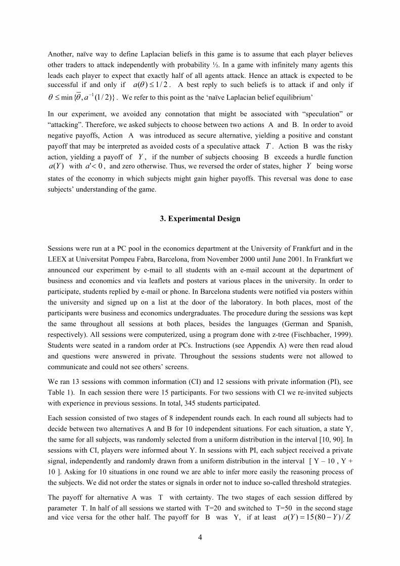
subjects chose B, zero otherwise. The formula was written in the instructions, but also explained with an example and a table (see Appendix A). In four sessions we applied Z=100, in the others Z=60. All parameters of the game and the rules were common information except for drawn states Y and private signals in the PI sessions. Table 1 gives an overview of the different sessions.

Number of sessions with Z

Secure payoff T

Location

Experienced subjects

Public information Private information

100 1rst stage 20 /2nd stage 50 Frankfurt No 1 1

100 50 / 20 Frankfurt No 1 1

60 20 / 50 Frankfurt No 1 2

60 20 / 50 Barcelona No 3 3

60 50 / 20 Frankfurt No 2 2

60 50 / 20 Barcelona No 3 3

60 20 / 50 Frankfurt Yes 1

60 50 / 20 Frankfurt Yes 1

Total number of sessions 13 12 Table 1. Session overview.

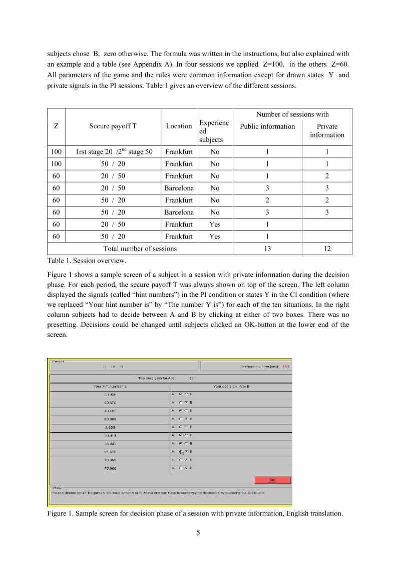
Figure 1 shows a sample screen of a subject in a session with private information during the decision phase. For each period, the secure payoff T was always shown on top of the screen. The left column displayed the signals (called “hint numbers”) in the PI condition or states Y in the CI condition (where we replaced “Your hint number is” by “The number Y is”) for each of the ten situations. In the right column subjects had to decide between A and B by clicking at either of two boxes. There was no presetting. Decisions could be changed until subjects clicked an OK-button at the lower end of the screen.

Figure 1. Sample screen for decision phase of a session with private information, English translation.

6

Once all players had completed their decisions in one round, they were informed for each situation about their own private signal (in PI-sessions), about Y (true value), their choice, how many people had chosen B, whether the decision B was successful or not, their individual payoffs and the cumulative payoff over all 10 situations (see Figure 2). After all players had left the information screen a new period started and information of previous periods could not be revisited.4 Subjects were allowed to take notes and many of them did.

Figure 2. Sample screen for information phase of a session with private information, English translation.

At the end of each session participants had to write in a questionnaire (via computer) their personal data, respond to four questions about their behavior and were free to give additional comments regarding the experiment. Once completed the questionnaire, each person was paid in private converting their total points into DM and Pesetas, respectively. In sessions with Z=100: 250 ECU = 1 DM=0,51 €. In sessions with Z = 60, 200 ECU were converted to1 DM (0,51 €) in Frankfurt and to70 Ptas (0,42 €) in Barcelona. Average payment per subject varied across sessions from 34 to 44 DM (17 to 22 Euros) in Frankfurt and from 2380 to 3140 Pesetas (14 to 19 Euros) in Barcelona. Session length was between 90 and 120 minutes.

4 Within the decision phase a descending clock at the top of the screen indicated the time left. However, at the time limit subjects were only reminded to make their decision with no other consequence. In the information phase reaching the time limit meant that the screen vanished and the next period started. Time limits were originally set to 180 seconds for a decision phase and 150 seconds for the information phase. After many students showed signs of boredom in the first sessions with CI, we reduced time limits in the second treatment of sessions with CI by 30 seconds.

7

4. Theoretical Predictions

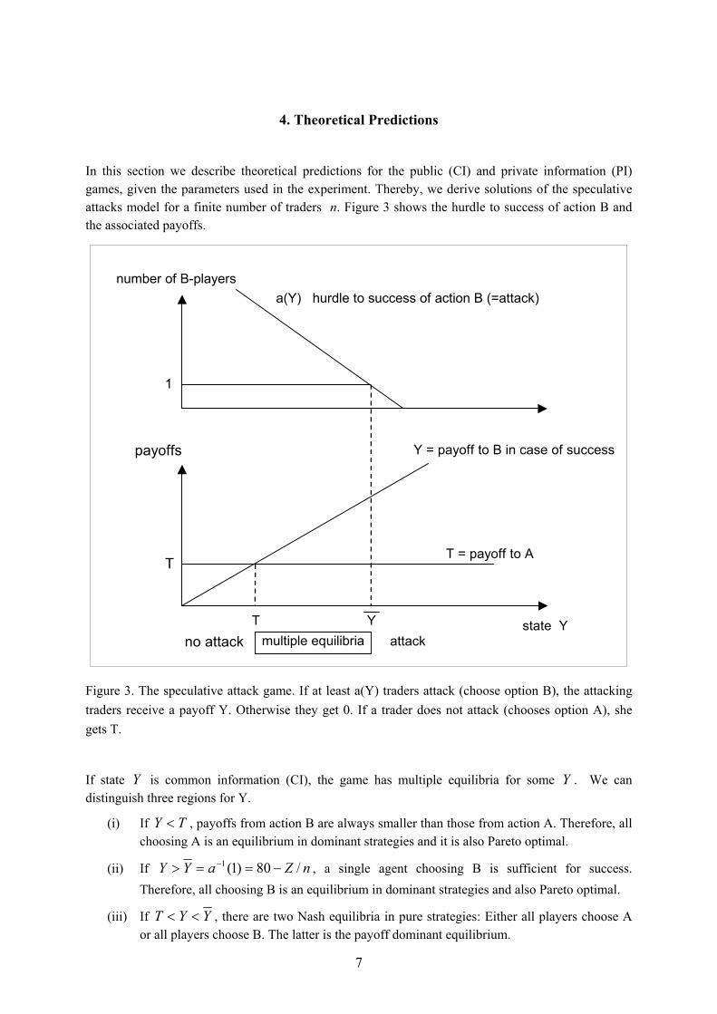
In this section we describe theoretical predictions for the public (CI) and private information (PI) games, given the parameters used in the experiment. Thereby, we derive solutions of the speculative attacks model for a finite number of traders n. Figure 3 shows the hurdle to success of action B and the associated payoffs.

state Y

payoffs

number of B-players

T = payoff to AT

Y = payoff to B in case of success

T

1

a(Y) hurdle to success of action B (=attack)

Ymultiple equilibriano attack attack

Figure 3. The speculative attack game. If at least a(Y) traders attack (choose option B), the attacking traders receive a payoff Y. Otherwise they get 0. If a trader does not attack (chooses option A), she gets T.

If state Y is common information (CI), the game has multiple equilibria for some Y . We can distinguish three regions for Y.

(i) If TY < , payoffs from action B are always smaller than those from action A. Therefore, all choosing A is an equilibrium in dominant strategies and it is also Pareto optimal.

(ii) If nZaYY /80)1(1 −==> − , a single agent choosing B is sufficient for success. Therefore, all choosing B is an equilibrium in dominant strategies and also Pareto optimal.

(iii) If YYT << , there are two Nash equilibria in pure strategies: Either all players choose A or all players choose B. The latter is the payoff dominant equilibrium.

8

A refinement theory selects a unique threshold state up to which all players choose A and above which all players choose B.

The payoff dominant equilibrium, recommended by Harsanyi and Selten (1988), prescribes B, if and only if TY > and hence the threshold state is Y=T.

The maximin strategy prescribes B if and only if success does not depend on other subjects’ decisions. Thus, the threshold state is YY = .

In the game with private information (PI), there is a unique equilibrium with a threshold signal *X , such that a risk neutral player with *X is indifferent between choosing A or B provided that all other players choose B if and only if they receive signals above *X . At state Y the probability of getting payoff Y for action B is given by the probability that at least 1)( −Ya out of the other 1−n players get signals above *X and choose B. This can be described by the binomial distribution. The probability that a single player gets a signal above *X at state Y is )2(/)( * εε+− XY . Denoting the round-up of )(Ya by )(ˆ Ya , expected utility of an agent choosing B is

∫+

−

=ε

ε

*

*

)( *X

XB YXU prob { }( )YYaXXij j 1)(|# * −≥>≠ dY

+−−−−= ∫

+

− εεε

ε 2,1,2)(ˆ1

**

*

XYnYaBinYX

X

dY ,

where Bin is the cumulative binomial distribution. The equilibrium threshold signal *X is defined by TXU B =)( * . For states in an ε -surrounding of *X the number of attacking agents and the success of an attack depend on the random draws of individual signals. Hence, there is no threshold state that divides successful from failed attacks for ε >0.

There are three further selection theories for the common information game based on players’ beliefs: For ε converging to zero, the threshold signal *X approaches a state Y* that may be interpreted as global game solution to the game with common information. As we explained in section 2, this state is the optimal threshold of a player who believes that the proportion of players who choose to attack has a uniform distribution in [0,1]. Therefore, we call it “Laplacian belief equilibrium”. If the proportion of other players choosing B has a uniform distribution, the probability of success of choice B by the

remaining player is n

Ya 1)(ˆ1 −− . At the equilibrium threshold state Y*, an agent is indifferent

between A and B. This threshold is the unique solution to [ ] TnYanY =+− 1)(ˆ .

The risk dominant equilibrium, as defined by Harsanyi and Selten (1988) differs slightly from the Laplacian belief equilibrium for 2>n . Here, each player acts as having second order beliefs, i.e., she believes that other players believe that the probability of success has a uniform distribution in [0,1]. Its threshold is given by the solution to ( )[ ] TYTnYaBinY =−−−− /1,1,2)(ˆ1 .

The threshold of the “naïve Laplacian equilibrium” is given by the state at which an agent is indifferent between A and B, when she believes that other players attack independently with probability ½. It is given by the solution to ( )[ ] TnYaBinY =−−− ½,1,2)(ˆ1 .

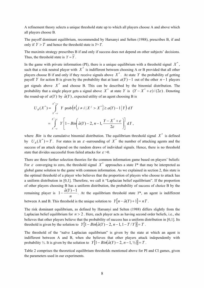
Table 2 comprises the theoretical equilibrium thresholds mentioned above for PI and CI games, given the parameters used in our experiments.

9

Treatments

Refinements

T=20, Z=100 T=20, Z=60 T=50, Z=100 T=50, Z=60

Payoff dominant equilibrium of CI game

20 20 50 50

Maximin equilibrium of the CI game

73.33 76.00 73.33 76.00

Unique equilibrium of PI game

32.36 41.84 60.98 66.03

Laplacian belief equilibrium of CI game

33.33 44.00 60.00 64.00

Risk dominant equilibrium of CI game

34.55 44.00 62.45 67.40

‘naïve’ Laplacian belief equilibrium of CI game

33.07 48.00 51.48 56.00

Table 2. Theoretical equilibrium threshold states or signals for the parameters T and Z, and n=15. .

5. Threshold Strategies

Each period subjects had to choose between A and B in 10 different situations that were given in random order. With this design, we are able to infer whether or not they used threshold strategies without imposing those strategies on the subjects. A subject’s behavior is consistent with a threshold strategy, if the highest state (in CI-treatments) or signal (in PI-treatments), for which the subject chose A, is smaller then the lowest state or signal, at which he or she chose B. Some subjects chose the same action for all signals/states in some periods, even when this action was dominated by the other for some signals/states. E.g. some subjects chose B when they should have known that TY < . In CI-treatments action B is dominated by A if Y < T and A is dominated by B if YY > . In PI-treatments B is dominated by A if signal Xi < T – ε and A is dominated by B if ε+> YX i . In most sessions, subjects who chose dominated actions in some rounds were the same as subjects whose behavior was inconsistent with a threshold after the second round. We call a subject’s behavior ‘consistent with undominated thresholds’ in some period, if her or his behavior in that period was consistent with existence of a threshold and did not exhibit any dominated actions.

Table 9 in Appendix B gives detailed account for the average number of subjects, whose behavior was consistent with undominated thresholds. In treatments with inexperienced subjects only, an average 92% of all strategies was consistent with undominated thresholds. We could not find any significant difference in the proportion of threshold strategies between sessions with common and private information, nor between treatments with different parameter values (see Table 9 and Regression 1 in Appendix C.3). In Barcelona the percentage of undominated threshold strategies appears to be significantly smaller than in Frankfurt using a simple Regression. Here, the location dummy is significant at the 5%-level and can explain 23% of the data variation (see Regression 2 in Appendix

10

C.3). We do not have an explanation for this difference. Table 9 in Appendix B shows, however, that in first and final rounds the difference between locations was small.

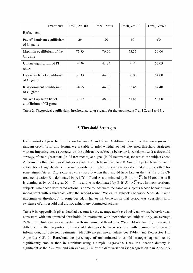
In the first round the number of inexperienced subjects employing undomintated thresholds varied from 5 to 14 for different sessions with an average of 10.78. In the second round, after they received information about their achieved payoffs and about aggregate behavior of other subjects, the number of undominated threshold strategies varied from 10 to 15. The average increased to 12.70. Some subjects seemed to need first feedback to understand the advantage of threshold strategies. Figure 4 shows that the proportion of undominated threshold strategies increased over time, although with the change of treatment in period 9, we observed this number to drop, especially in Barcelona. This may be due to confusion stemming from the parameter change. In all sessions we observed that during the last four periods at least 13 out of 15 participants employed undominated thresholds.

Evolution of Threshold Strategies

60%

70%

80%

90%

100%

1 2 3 4 5 6 7 8 9 10 11 12 13 14 15 16period

tres

hold

str

ateg

ies

private information

common information

Figure 4. Percentage of inexperienced subjects, whose behavior was consistent with undominated threshold strategies.

Two sessions with subjects, who had participated in one of the other sessions before (experienced subjects), showed a higher proportion of threshold strategies (97%) than sessions with subjects, who participated for the first time (see Table 9 in Appendix B). However, the selection of subjects, who agreed to participate a second time, is endogenous, and results must be compared with caution.

On one hand, it is not surprising that most participants played threshold strategies: The hurdle for success of B is decreasing in Y , the payoff to B in case of success is increasing. However, deductive reasoning needs very strong assumptions to get this result: In games with private information, theory predicts threshold strategies but requires common knowledge of the game structure. In games with common information non-threshold strategies may even occur in Nash equilibria.

11

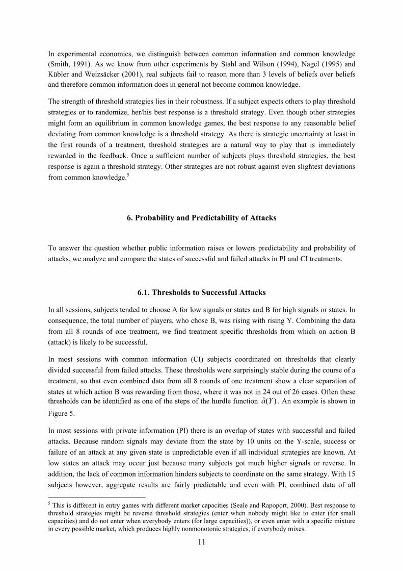
In experimental economics, we distinguish between common information and common knowledge (Smith, 1991). As we know from other experiments by Stahl and Wilson (1994), Nagel (1995) and Kübler and Weizsäcker (2001), real subjects fail to reason more than 3 levels of beliefs over beliefs and therefore common information does in general not become common knowledge.

The strength of threshold strategies lies in their robustness. If a subject expects others to play threshold strategies or to randomize, her/his best response is a threshold strategy. Even though other strategies might form an equilibrium in common knowledge games, the best response to any reasonable belief deviating from common knowledge is a threshold strategy. As there is strategic uncertainty at least in the first rounds of a treatment, threshold strategies are a natural way to play that is immediately rewarded in the feedback. Once a sufficient number of subjects plays threshold strategies, the best response is again a threshold strategy. Other strategies are not robust against even slightest deviations from common knowledge.5

6. Probability and Predictability of Attacks

To answer the question whether public information raises or lowers predictability and probability of attacks, we analyze and compare the states of successful and failed attacks in PI and CI treatments.

6.1. Thresholds to Successful Attacks

In all sessions, subjects tended to choose A for low signals or states and B for high signals or states. In consequence, the total number of players, who chose B, was rising with rising Y. Combining the data from all 8 rounds of one treatment, we find treatment specific thresholds from which on action B (attack) is likely to be successful.

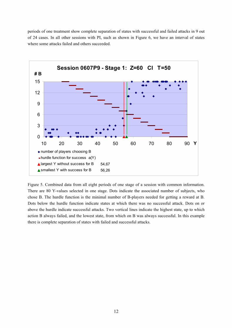
In most sessions with common information (CI) subjects coordinated on thresholds that clearly divided successful from failed attacks. These thresholds were surprisingly stable during the course of a treatment, so that even combined data from all 8 rounds of one treatment show a clear separation of states at which action B was rewarding from those, where it was not in 24 out of 26 cases. Often these thresholds can be identified as one of the steps of the hurdle function )(ˆ Ya . An example is shown in

Figure 5.

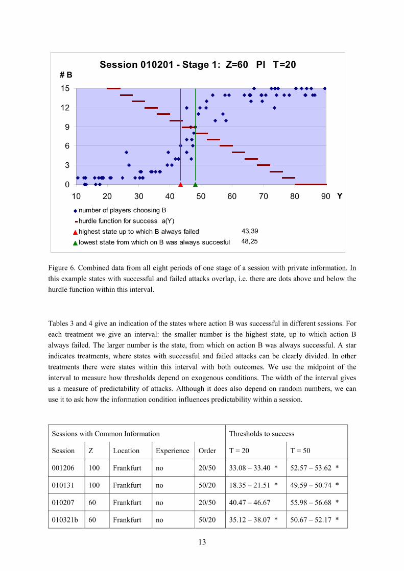
In most sessions with private information (PI) there is an overlap of states with successful and failed attacks. Because random signals may deviate from the state by 10 units on the Y-scale, success or failure of an attack at any given state is unpredictable even if all individual strategies are known. At low states an attack may occur just because many subjects got much higher signals or reverse. In addition, the lack of common information hinders subjects to coordinate on the same strategy. With 15 subjects however, aggregate results are fairly predictable and even with PI, combined data of all

5 This is different in entry games with different market capacities (Seale and Rapoport, 2000). Best response to threshold strategies might be reverse threshold strategies (enter when nobody might like to enter (for small capacities) and do not enter when everybody enters (for large capacities)), or even enter with a specific mixture in every possible market, which produces highly nonmonotonic strategies, if everybody mixes.

12

periods of one treatment show complete separation of states with successful and failed attacks in 9 out of 24 cases. In all other sessions with PI, such as shown in Figure 6, we have an interval of states where some attacks failed and others succeeded.

Session 0607P9 - Stage 1: Z=60 CI T=50

54,6756,26

0

3

6

9

12

15

10 20 30 40 50 60 70 80 90 Y

# B

number of players choosing Bhurdle function for success a(Y)largest Y without success for Bsmallest Y with success for B

Figure 5. Combined data from all eight periods of one stage of a session with common information. There are 80 Y-values selected in one stage. Dots indicate the associated number of subjects, who chose B. The hurdle function is the minimal number of B-players needed for getting a reward at B. Dots below the hurdle function indicate states at which there was no successful attack. Dots on or above the hurdle indicate successful attacks. Two vertical lines indicate the highest state, up to which action B always failed, and the lowest state, from which on B was always successful. In this example there is complete separation of states with failed and successful attacks.

13

Session 010201 - Stage 1: Z=60 PI T=20

43,3948,25

0

3

6

9

12

15

10 20 30 40 50 60 70 80 90 Y

# B

number of players choosing Bhurdle function for success a(Y)highest state up to which B always failedlowest state from which on B was always succesful

Figure 6. Combined data from all eight periods of one stage of a session with private information. In this example states with successful and failed attacks overlap, i.e. there are dots above and below the hurdle function within this interval.

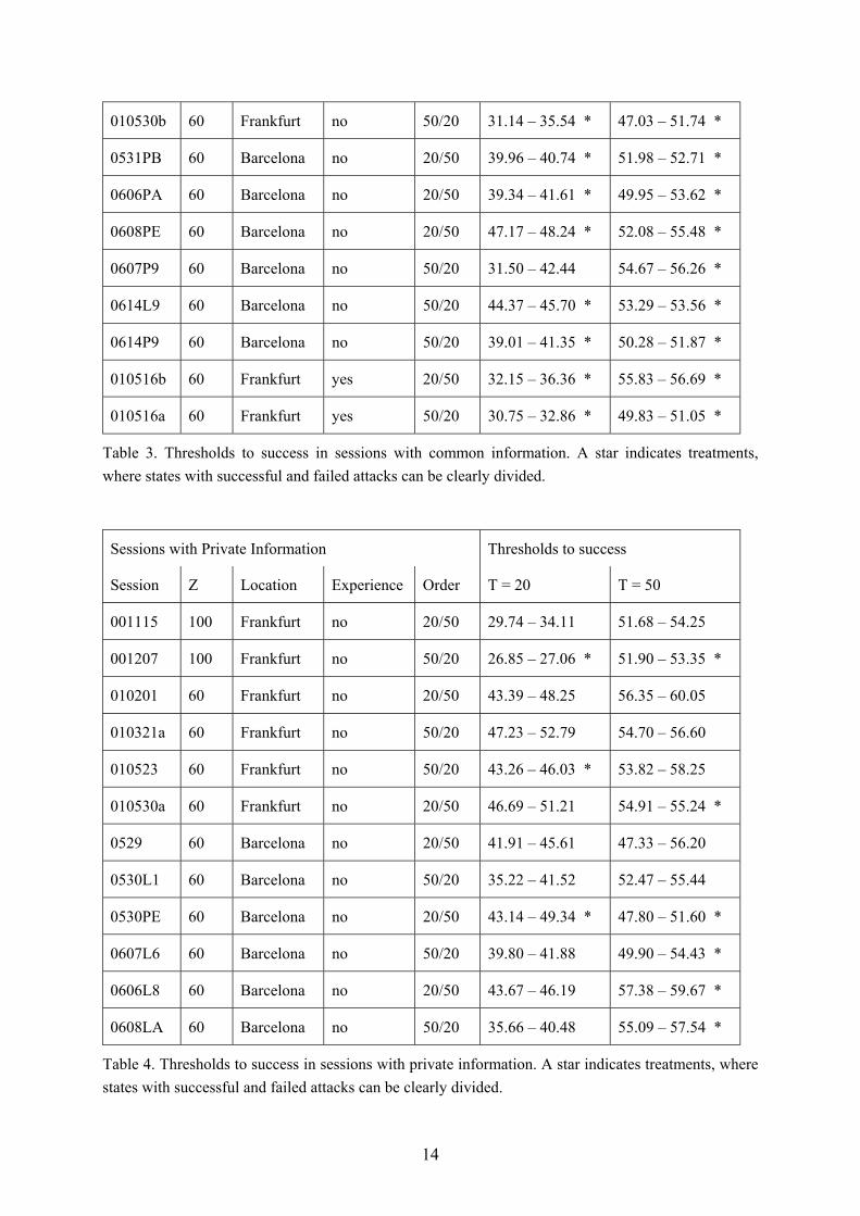
Tables 3 and 4 give an indication of the states where action B was successful in different sessions. For each treatment we give an interval: the smaller number is the highest state, up to which action B always failed. The larger number is the state, from which on action B was always successful. A star indicates treatments, where states with successful and failed attacks can be clearly divided. In other treatments there were states within this interval with both outcomes. We use the midpoint of the interval to measure how thresholds depend on exogenous conditions. The width of the interval gives us a measure of predictability of attacks. Although it does also depend on random numbers, we can use it to ask how the information condition influences predictability within a session.

Sessions with Common Information Thresholds to success

Session Z Location Experience Order T = 20 T = 50

001206 100 Frankfurt no 20/50 33.08 – 33.40 * 52.57 – 53.62 *

010131 100 Frankfurt no 50/20 18.35 – 21.51 * 49.59 – 50.74 *

010207 60 Frankfurt no 20/50 40.47 – 46.67 55.98 – 56.68 *

010321b 60 Frankfurt no 50/20 35.12 – 38.07 * 50.67 – 52.17 *

14

010530b 60 Frankfurt no 50/20 31.14 – 35.54 * 47.03 – 51.74 *

0531PB 60 Barcelona no 20/50 39.96 – 40.74 * 51.98 – 52.71 *

0606PA 60 Barcelona no 20/50 39.34 – 41.61 * 49.95 – 53.62 *

0608PE 60 Barcelona no 20/50 47.17 – 48.24 * 52.08 – 55.48 *

0607P9 60 Barcelona no 50/20 31.50 – 42.44 54.67 – 56.26 *

0614L9 60 Barcelona no 50/20 44.37 – 45.70 * 53.29 – 53.56 *

0614P9 60 Barcelona no 50/20 39.01 – 41.35 * 50.28 – 51.87 *

010516b 60 Frankfurt yes 20/50 32.15 – 36.36 * 55.83 – 56.69 *

010516a 60 Frankfurt yes 50/20 30.75 – 32.86 * 49.83 – 51.05 *

Table 3. Thresholds to success in sessions with common information. A star indicates treatments, where states with successful and failed attacks can be clearly divided.

Sessions with Private Information Thresholds to success

Session Z Location Experience Order T = 20 T = 50

001115 100 Frankfurt no 20/50 29.74 – 34.11 51.68 – 54.25

001207 100 Frankfurt no 50/20 26.85 – 27.06 * 51.90 – 53.35 *

010201 60 Frankfurt no 20/50 43.39 – 48.25 56.35 – 60.05

010321a 60 Frankfurt no 50/20 47.23 – 52.79 54.70 – 56.60

010523 60 Frankfurt no 50/20 43.26 – 46.03 * 53.82 – 58.25

010530a 60 Frankfurt no 20/50 46.69 – 51.21 54.91 – 55.24 *

0529 60 Barcelona no 20/50 41.91 – 45.61 47.33 – 56.20

0530L1 60 Barcelona no 50/20 35.22 – 41.52 52.47 – 55.44

0530PE 60 Barcelona no 20/50 43.14 – 49.34 * 47.80 – 51.60 *

0607L6 60 Barcelona no 50/20 39.80 – 41.88 49.90 – 54.43 *

0606L8 60 Barcelona no 20/50 43.67 – 46.19 57.38 – 59.67 *

0608LA 60 Barcelona no 50/20 35.66 – 40.48 55.09 – 57.54 *

Table 4. Thresholds to success in sessions with private information. A star indicates treatments, where states with successful and failed attacks can be clearly divided.

15

6.2. Probabilities of Successful Attacks

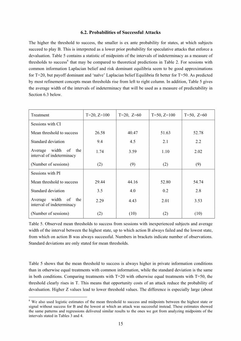
The higher the threshold to success, the smaller is ex ante probability for states, at which subjects succeed to play B. This is interpreted as a lower prior probability for speculative attacks that enforce a devaluation. Table 5 contains a statistic of midpoints of the intervals of indeterminacy as a measure of thresholds to success6 that may be compared to theoretical predictions in Table 2. For sessions with common information Laplacian belief and risk dominant equilibria seem to be good approximations for T=20, but payoff dominant and ‘naïve’ Laplacian belief Equilibria fit better for T=50. As predicted by most refinement concepts mean thresholds rise from left to right column. In addition, Table 5 gives the average width of the intervals of indeterminacy that will be used as a measure of predictability in Section 6.3 below.

Treatment T=20, Z=100 T=20, Z=60 T=50, Z=100 T=50, Z=60

Sessions with CI

Mean threshold to success 26.58 40.47 51.63 52.78

Standard deviation 9.4 4.5 2.1 2.2

Average width of the interval of indeterminacy

1.74 3.59 1.10 2.02

(Number of sessions) (2) (9) (2) (9)

Sessions with PI

Mean threshold to success 29.44 44.16 52.80 54.74

Standard deviation 3.5 4.0 0.2 2.8

Average width of the interval of indeterminacy

2.29 4.43 2.01 3.53

(Number of sessions) (2) (10) (2) (10)

Table 5. Observed mean thresholds to success from sessions with inexperienced subjects and average width of the interval between the highest state, up to which action B always failed and the lowest state, from which on action B was always successful. Numbers in brackets indicate number of observations. Standard deviations are only stated for mean thresholds.

Table 5 shows that the mean threshold to success is always higher in private information conditions than in otherwise equal treatments with common information, while the standard deviation is the same in both conditions. Comparing treatments with T=20 with otherwise equal treatments with T=50, the threshold clearly rises in T. This means that opportunity costs of an attack reduce the probability of devaluation. Higher Z values lead to lower threshold values. The difference is especially large (about

6 We also used logistic estimates of the mean threshold to success and midpoints between the highest state or signal without success for B and the lowest at which an attack was successful instead. These estimates showed the same patterns and regressions delivered similar results to the ones we got from analyzing midpoints of the intervals stated in Tables 3 and 4.

16

14) for T=20 and Z=100 compared to T=20 and Z=60 (see first and second column); with T=50 the difference is only 2 (third and fourth column). This is partially due to the non-linear payoff function. In the interpretation by Morris and Shin (1998) and Heinemann (2000) the effect of the hurdle function means that capital controls reduce the probability of successful attacks.

For a systematic analysis of the influence of information and other controls variables on mean thresholds we use linear regressions (see Appendix C.2). To control for the non-linearity in the payoff function, our regressions include an interaction variable TZ that equals one if and only if T=50 and Z=60. Regression 3 shows that T and Z explain 82% of all data variation. Regression 4 shows that information, location, and the order of treatments increase this to 89%.

With common information thresholds tend to be 2.45 units lower than with private information. This difference is numerically small, but significant at 2%. Given the stochastic framework used for our experiment, a commitment to provide public information at any state increases the prior probability of devaluation by 3.1%7.

In sessions with private information, thresholds were higher in Frankfurt than in Barcelona. In sessions with common information it was the other way round, but not significant (see Regressions 5 and 6).

Surprisingly, thresholds tend to be higher in sessions, where we started with a low payoff for the secure action (T=20) than in sessions, where we started with a high payoff (T=50). Originally we expected the opposite result. With numerical inertia, the threshold for T=20 should be higher after a treatment with T=50 than in a session that starts with T=20. After a treatment with T=20 the threshold for T=50 should be lower than in a session that starts with T=50. But, we observe thresholds in treatments with T=20 to be lower after a treatment with T=50 by some 5 units. In treatments with T=50 thresholds are about 1 unit higher, when they were preceded by a treatment with T=20.8 There are different possible explanations: The order effect could be due to subjects having more trust in the ability of the group to coordinate after observing coordination close to T in treatments with T=50, where the hurdle to success a(Y) requires a smaller number of players. A formal way to express this is suggested by answers in the questionnaire. Many subjects reported that they played B for all signals or states that were some increment iδ above T, where iδ was sometimes reported as being 10 or 20 and gradually adjusted with experience. The order effect is consistent with a numerical inertia in these increments iδ . After observing a threshold close to T=50, where the hurdle to success a(Y) requires a smaller number of B-players, the increment was low and subjects may have tried to attack at states close to T=20 in the second stage. Subjects who start with T=20 do not get that close to the payoff dominant equilibrium, because here, the hurdle is higher. Taking their experience in form of a high increment to the second stage, at which T=50, thresholds to attack are higher than for subjects who start with T=50.

7 Since states have a uniform distribution on [10,90], a reduction of the threshold by 2.45 increases the probability of states exceeding the threshold by 2.45 / 80 = 3.1% 8 The difference in the numerical impact that the order of treatments has on thresholds for T=20 and T=50, respectively, is accounted for by the interaction variable TO in the regressions.

17

6.3. Predictability of Attacks

Here, we ask whether there is any difference in predictability of thresholds related to the information condition. Comparing the standard deviations of average thresholds in Table 5 above, it seems that the information condition has no big impact on the dispersion of observed thresholds among otherwise equal treatments. This impression is supported by separate regressions of thresholds for both information conditions. In sessions with common information 91% of all data variation can be explained by the other controlled variables (see Regression 5). In sessions with private information other controlled variables explain 93% of data variation (see Regression 6). However, the standard variation of residuals is 2.84 in sessions with common and 4.63 in sessions with private information. If thresholds have a normal distribution, they can be predicted within an interval of four standard deviations with a probability of 95%. We see clearly that this interval is larger with private than with common information.

Even though thresholds are fairly predictable for both scenarios, there may be differences in predictability within a session. This can be measured by the width of the interval between the highest state, up to which action B always failed, and the lowest state, from which on action B was always successful (see Table 5 in Section 6.2). These intervals tend to be wider for a steep hurdle function (Z=60) and also for private information. Note that average distance between two neighbouring states is 0.99.9

On average over all treatments with common information the interval of states for which there is no clear indication of whether attacks fail or succeed has width 2.55. In treatments with private information its width is 3.68 on average. Regressions 7 and 8 (Appendix C.3) show that this difference in information conditions is just on the edge to significance at a 10%-level. If this difference is real, private information increases the range of states for which we cannot predict whether an attack is successful or not by 1.13. Accordingly, with PI the prior probability that a state falls into the region of indeterminacy rises from 3.2% to 4.6%.

In fact, this method underestimates predictability in CI-conditions and overestimates it in PI-conditions. In sessions with CI, subjects consciously coordinate on a common threshold. In at least 18 out of 26 treatments with CI, we have the impression that subjects coordinated on a step of the hurdle function. With a high degree of coordination the probability that an attack is successful at any state below the given interval (or fails at a state above it) is zero. With random signals in the PI setting, this probability is inevitably positive. Thus, with private information predictability is even lower than the width of the interval indicates.

With public information the central bank has more control on the beliefs of traders than if they get private information from other sources. Uncontrolled information reduces the ability of the central bank to predict an attack. This loss in predictability that is modelled by the random nature of private information in our experiment outweighs the loss of predictability that might occur with public information due to self-fulfilling beliefs. The results of our experiment indicate that both effects are small when the number of traders is sufficiently large. For games with fewer players, both effects might gain importance and it is an open question which one is bigger with fewer subjects.

9 With 80 values of Y, independently drawn from a uniform distribution on [10,90].

18

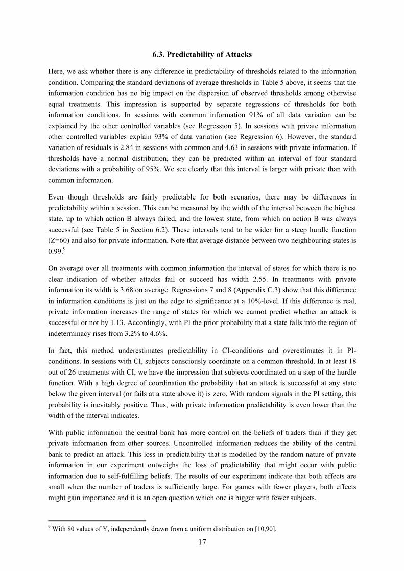
6.4. Coordination Failures

When individual behaviour is not perfectly coordinated, subjects experience mistakes in the information phase and learn to adjust their thresholds towards each other. There are two possible situations in which a subject could regret her decision: (i) she chose B and received 0 (a failed attack), (ii) she chose A, when B would have given a higher reward (a missed opportunity to attack). These situations should not occur, when a subject can predict whether an attack will be successful or not. The total number of cases where subjects could regret their decisions give us a measure for their ability to predict whether an attack will be successful or not.

Figure 7 shows the average number of decisions where a subject could have improved her payoff by deciding differently. In sessions with CI this number has a clear trend to decrease over time. Subjects learn to coordinate on or better predict a common threshold. They learn to play a Nash Equilibrium. When their behavior is fully coordinated, they never regret any decision. The change of treatment in period 9 increases again the number of regrets and subjects have to find a new coordination point. In sessions with private information the average number of regrets decreases for the first 3 periods and bounces around 1.0 thereafter.

With private information there are more regrettable decisions than with common information from the second round of a treatment onwards. This tells us that once subjects gained some experience with a treatment, they could better predict the outcome in CI sessions. This is mainly due to randomness of signals. Random nature of signals in the PI-condition leads to an expected number of regrettable decisions of about 0.6-0.7, even if all subjects play the same threshold strategy.10 The difference between observed and expected number of regrets under perfect coordination is of the same size as in the CI condition. Surprisingly, with PI this number does not even increase after the change of treatment. So, given the external conditions, subjects ability to predict an attack is not affected by the information condition. There is no publicity multiplier associated with CI that might increase their ability to predict aggregate behavior of other subjects beyond the reduction in exogenous uncertainty.

10 The expected number of failures in the Nash equilibrium of a PI game depends on parameters T and Z and can be estimated by Monte Carlo simulations. It varies in the range 0.6-0.7 for our treatments.

19

Evolution of Coordination

0,00,20,40,60,81,01,21,41,61,82,0

1 2 3 4 5 6 7 8 9 10 11 12 13 14 15 16

Period

aver

age

num

ber o

f reg

retta

ble

deci

sion

s

regrettable decisions in sessions with PI

regrettable decisions in sessions with CI

Figure 7. Average number of situations in which a subject could have achieved a higher payoff by a different decision.

7. Testing Equilibrium Refinements

In this section we test the explanatory power of various refinement concepts. For this we first estimate mean individual thresholds with logistic regressions.

7.1. Mean Thresholds of Individual Strategies

When all subjects employ threshold strategies, the proportion of agents who are choosing B is an increasing function in states or signals that can be estimated by fitting a distribution function to these data. The logistic distribution is more appropriate than the normal distribution, because we observe ‘fat tails’ due to irrational behavior of few subjects who do not play threshold strategies.

We estimate the distribution of thresholds for each session using a logistic estimation. Estimates based on single periods do not show much variation after the first three periods of each treatment. This is in line with a general impression that individual behavior does not change much after the first periods. Therefore, we can improve the quality of estimates by combining data of the last four rounds of each treatment. Results are logistic distributions that may be interpreted in two ways: (i) as estimated probabilities for subjects choosing B conditional on state Y or signal X, respectively, (ii) as estimated distribution of individual thresholds. Figures 8 and 9 give an impression of the data fit obtained by

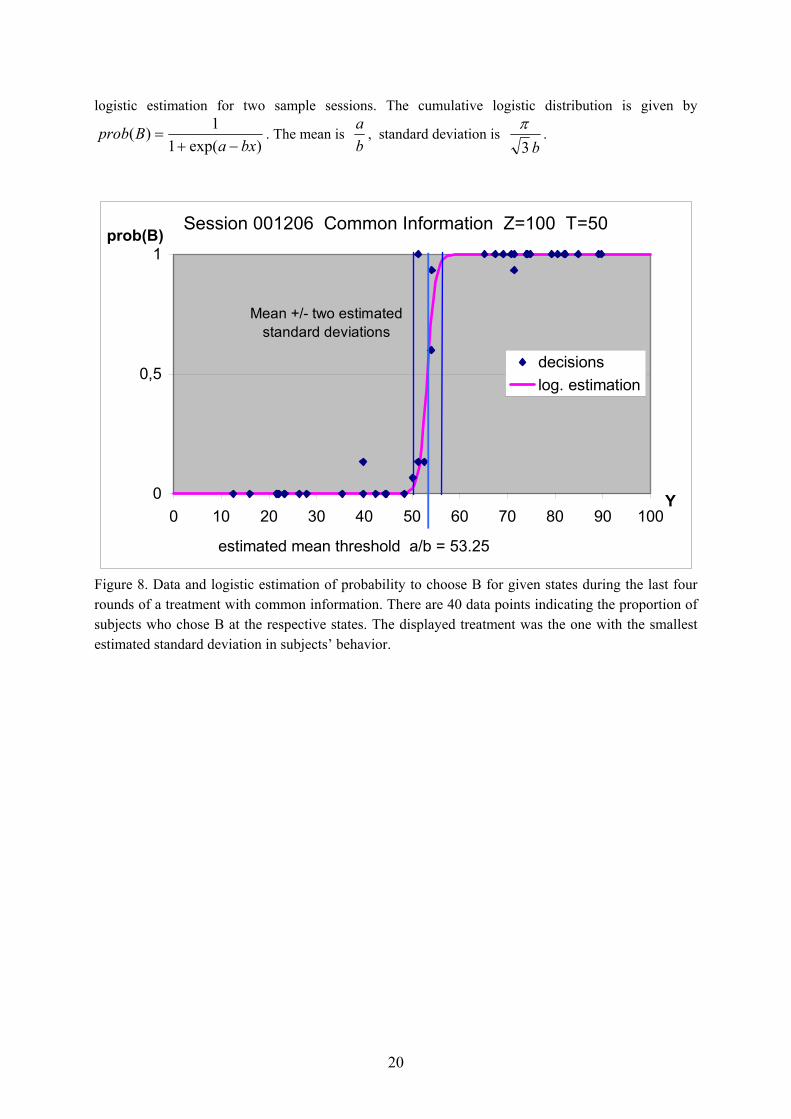
20

logistic estimation for two sample sessions. The cumulative logistic distribution is given by

)exp(11)(

bxaBprob

−+= . The mean is

ba

, standard deviation is b3

π.

Session 001206 Common Information Z=100 T=50

0

0,5

1

0 10 20 30 40 50 60 70 80 90 100Y

prob(B)

decisionslog. estimation

estimated mean threshold a/b = 53.25

Mean +/- two estimated standard deviations

Figure 8. Data and logistic estimation of probability to choose B for given states during the last four rounds of a treatment with common information. There are 40 data points indicating the proportion of subjects who chose B at the respective states. The displayed treatment was the one with the smallest estimated standard deviation in subjects’ behavior.

21

Session 010201 Private Information Z=60 T=20

0

0.5

1

0 10 20 30 40 50 60 70 80 90 100X

prob(B)

decisionslog. estimation

estimated mean threshold a/b = 46.40

Mean +/- one estimated standard deviation

Figure 9. Data and logistic estimation of probability to choose B for given signals during the last four rounds of a treatment with private information. There are 600 data points indicating subjects’ decisions (B=1) at their respective signals. The displayed treatment was the one with the largest estimated standard deviation in subjects’ behavior. Detailed results of logistic regressions (based on decisions in the last four rounds of each treatment) for all sessions and treatments are displayed in Appendix C.4. Table 6 gives a summery statistic of

estimated means ba / and estimated standard deviations b3

π of individual thresholds for

distinguished treatments. Treatment T=20, Z=100 T=20, Z=60 T=50, Z=100 T=50, Z=60

Sessions with CI

Average estimated mean of individual thresholds

26.30 37.84 52.96 52.56

Average estimated standard deviation Number of sessions

5.30

2

7.94

9

5.71

2

7.56

9

Sessions with PI Average estimated mean of individual thresholds

29.76 41.95 55.22 57.02

Average estimated standard deviation Number of sessions

8.81

2

10.05

10

9.46

2

9.77

10 Table 6. Average estimated means and standard deviations of individual thresholds to action B in sessions with inexperienced subjects.

22

Similar to the analysis of thresholds to successful attacks in Section 6.2, we run linear regressions using the controlled variables to explain mean thresholds and standard deviations of individual thresholds within each treatment. Appendix C.5 displays results for two of these regressions. Regression 9 shows significant influence on the estimated mean threshold (a/b) by the parameters of the payoff function T and Z, by the information scenario, and by the order of treatments. All of these effects are very similar to their influence on the threshold to success in Regression 2. The information condition has an even stronger impact on the mean of individual thresholds than on the critical state to success. Note, that the mean of individual thresholds depends on the behavior of subjects with extreme strategies, while the threshold state to success does not.

Non-parametric tests also show a significant difference between sessions with different information and order of treatments. Here, we had to use separate tests for each T. While information and order of treatments were significant at 5% in Mann-Whitney-Tests for both T-values, information failed to be significant at 5% for Kolmogoroff-Smirnov-Tests.

Regression 10 shows that the estimated dispersion of individual thresholds as measured by the standard deviations of the logistic distributions is significantly larger with private than with common information. It is also larger in sessions starting with T=20 than in the second stage of a session that had started with T=50. The standard deviation of individual thresholds within a session is another measure of coordination. The higher this standard deviation is, the less are subjects’ decisions coordinated. This is another proof that CI improves the ability of subjects to coordinate their strategies.

When we include sessions with experienced subjects, we observe that experience lowers the mean threshold by about 2.6. But, with only four data points for experienced subjects, this difference fails to be significant.

7.2. Testing Theoretical Equilibria

As mentioned in section 4, different theoretical equilibrium concepts define different threshold states or signals. In this section we ask whether observed behavior is in line with any of the theoretical equilibrium concepts. We have seen already that there is some dispersion in actual individual strategies that should not occur in equilibrium, when all subjects employ the same strategy. But, there is another interpretation of equilibria: Even if individual strategies differ, refinement theories might succeed in describing the average behavior of individuals. We test whether mean individual thresholds are either of the theoretically predicted equilibrium thresholds.

We use a two sided F-test on the difference between estimated mean individual thresholds as derived by logistic regressions in Appendix C.4 and theoretical predictions given in Section 4, Table 2. Appendix D lays out an example of the test procedure. We have 11 sessions of 2 stages each with common information and inexperienced subjects, generating 22 data points for these treatments. We use these data to test payoff dominance, Laplacian beliefs, risk dominance, ‘naïve’ Laplacian beliefs and maximin strategies. In 12 sessions inexperienced subjects had private information, generating 24 data points for testing the equilibrium of the private information game. Appendix D exhibits precise results of these tests.

The hypothesis that subjects play Maximin strategies can be most clearly rejected, as all estimated mean thresholds are far below the thresholds associated with Maximin strategies.

23

The hypothesis that subjects play the payoff dominant equilibrium in sessions with common information is rejected at the 1% level if we jointly use data from treatments with T=20 and T=50. However, for T=50 estimated thresholds come rather close to the payoff dominant equilibrium. Using data from treatments with T=50 only, the p-value for rejection is at 4%.

The hypotheses that subjects play the Laplacian belief or the risk dominant equilibrium can be rejected at a p-level of 1%. Table 14 (Appendix C.4) reveals that estimated mean thresholds are below these equilibria in all treatments with common information.

The hypotheses that subjects play the ‘naïve’ Laplacian belief equilibrium can be rejected for all data with Z=60 and for all data with T=20. For data with T=50, the p-value was at 6.8% and does not allow rejection.

The hypothesis that subjects play the unique equilibrium in games with private information is rejected at the 1% level when we use all data from sessions with Z=60. However, for data from treatments with T=20, we can not reject it. In fact, it seemed a pretty good predictor here with estimated mean thresholds being distributed around the equilibrium. For T=50 these estimates are all clearly below the equilibrium.

In Section 6.2 above, we pointed out that average thresholds were higher for higher T or lower Z. This is actually another reason to reject payoff dominance or minimax strategies, because the payoff dominant equilibrium does not depend on Z and the minimax strategy does not depend on T. The other theoretical equilibria follow these parameter changes in the observed direction.

Finally, we test the predictive power of refinements on aggregate by comparing whether observed thresholds to successful attacks (see Section 6.1) are in a neighborhood of various theoretical equilibria. Results of this heuristic procedure are summarized in Table 7. The success rate indicates the percentage of treatments from sessions with CI and inexperienced subjects, in which revealed threshold intervals given in Table 3 overlap with a neighborhood of 2 around theoretical equilibria from Table 2.

Equilibrium All 22 observations T=20 (11 obs.) T=50 (11 obs.)

Payoff dominant equilibrium 36% 9% 64%

Laplacian belief equilibrium 18% 36% 0

Risk dominant equilibrium 18% 36% 0

‘naïve’ Laplacian belief equil. 32% 18% 45%

Maximin Strategy 0 0 0

neither of the above 27% 45% 9%

Table 7. Success rates of theoretical equilibrium thresholds in CI-games +/– 2.

While observed behavior came rather close to payoff dominance in treatments with T=50, risk dominance and Laplacian beliefs were a better approximation to behavior for T=20. The reason might be the higher number of subjects needed for success at low values of Y.

Surprisingly, ‘naïve’ Laplacian beliefs did not bad in this comparison. We can even do better, if we replace the belief that other players choose B with probability ½ by higher probabilities. Maximizing

24

the success rate (as defined above) leads to beliefs of some 0.6 – 0.7 for other players choosing B. To be more precise, if each player beliefs that each other player chooses B with probability p, the best response is a threshold Y, solving ( )[ ] TpnYaBinY =−−− ,1,2)(ˆ1 . If we take p = 2/3, we get

equilibrium thresholds and according success rates as displayed in Table 10.

Parameters Z=100, T=20 Z=60, T=20 Z=100, T=50 Z=60, T=50

Best response threshold to p=2/3

23.515 40.00 50.035 52.00

Success cases 0 out of 2 6 out of 9 1 out of 2 7 out of 9

Success rate 54% 73%

Table 8. Best response thresholds to belief that other players choose B with probability 2/3 and success rates of these thresholds +/– 2.

The overall success rate of thresholds that are a best response to p = 2/3 is 64%. Table 8 shows, how this success rate varies between treatments. The overall success rate does not change for p ∈ [0.6, 0.68] and is lower for any p outside this interval. In F-tests the hypothesis that subjects play a best response to p=2/3 could not be rejected, while all the other theoretical equilibria could (see Appendix D). However, this is not a fair test, as we did not plan to test this equilibrium beforehand, but rather arrived at it endogenously.

Thresholds, associated with a best response to subjects believing that others choose B with probability p=2/3 can explain observed behavior in sessions with common information very well. This might be an artifact of our experiment and might just hold for sessions with Z=60. But, it might also be possible that this opens a way to measure strategic uncertainty in binary choice games by maximum likelihood estimates of first order beliefs.

8. Comparison with Previous Experiments and Conclusions

Previous experiments on coordination games with strategic complementarities have shown that we should distinguish between two kinds of coordination: Coordination on an equilibrium and coordination on the efficient equilibrium. Comparing our results with those of Van Huck, Battaglio und Beil (1990, 1991), we find some similarities and some additional insights:

- As in their experiment, we find a fast convergence towards an equilibrium in sessions with common information.

- Groups of 14 – 16 did never succeed to reach an equilibrium better than maximin-strategies in the experiment of Van Huyck et al. (1990), where all members were needed to coordinate for this purpose, while coordination by two players was achieved even in a random matching. In our experiment, we never observed an equilibrium that needed coordination of more than 12 out of 15 subjects.

- In their median treatments, behavior always converged to an equilibrium determined by the median of the first round, hinting at strong inertia effects. In our game, it should be easier to

25

observe changes in the equilibrium played, because of random draws, continuous strategy space and information on the number of B-players at various states. Even so, in 24 out of 26 treatments with CI, we do not observe the threshold for success of action B to move. In only two sessions, there is a slight change of the threshold after the first round of a treatment.

- A change of treatment and associated experience with coordination, led subjects to play more efficient equilibria in Van Huyck et al. (1991). We observed similar effects: Experience lowered average thresholds and the order effect might also be explained by experience with coordination as explained at the end of Section 6.2.

- Van Huyck et al. found that subjects coordinate on equilibria that are somewhere between maximin-strategies and the payoff dominant equilibrium. However, in their game maximin- and risk dominant strategies coincid. In our experiment, all observed equilibria were between the risk dominant and the payoff dominant equilibrium.

In a previous experiment on global games by Cabrales, Nagel and Armenter (2002) subjects reached the risk dominant equilibrium and there were no apparent differences in behavior between sessions with common and private information. However, their stage game had only five possible states and signals and may have been too discrete to discover the subtle effects of information. In our game, with a continuous space for states and signals, we observe that with common information, coordination of agents was much better than with private information. In addition, the average threshold, and thus, the prior probability of failure of the risky action, was significantly higher with private information. On the other hand, we do not find any significant difference in the proportion of subjects using threshold strategies or in the dispersion of achieved mean thresholds across different sessions. This leads us to conclude that the interpretation of multiple equilibria as an indication for a destabilizing effect of public information is not warranted.

However, public information leads players to coordinate on an equilibrium with a higher payoff. Reduced exogenous uncertainty leads them to engage in strategies that bear a larger strategic risk, because success requires coordination of a larger number of players.

In our view, strategic uncertainty is the major force that drives subjects to play threshold strategies, explains the low variation of observed equilibria in common information games, and also explains most of the comparative statics. We think that the deviation of observed behavior in sessions with private information from Nash equilibrium into the direction of ‘naïve’ Laplacian beliefs might also be due to strategic uncertainty that adds to exogenous uncertainty in these games. Even though we could reject all pre-selected equilibrium concepts, the concepts that considered both, possible gains from coordination as well as the hurdle to achieve these gains, did best in predicting observed comparative statics. In particular, the equilibrium that we called ‘Laplacian belief equilibrium’, introduced by Carlsson and van Damme (1993a) and Morris and Shin (2000) as limiting equilibrium of global games for diminishing uncertainty of private information, combines the advantages to exhibit observed comparative statics and to be easy to calculate. Risk dominance is difficult to calculate in some games, but is not limited to coordination games. The ‘naïve’ Laplacian belief equilibrium leads to strange results for some games, especially for a large number of players and lacks a theoretical justification.

The current discussion on the optimal modes of information disclosure concentrates on the multiplicity of equilibria associated with public information. Our experiment suggests that this may be a subordinate effect. Thresholds to successful speculative attacks were fairly predictable for both information conditions. The major effect might be that public information reduces the threshold to attack, and a commitment to provide public information raises the prior probability of currency crises.

26

Public information directs strategies towards the payoff dominant equilibrium. Payoff dominance may be desirable for some coordination games. For others, it may be the opposite. In order to avoid speculative attacks, a central bank should minimize expected gains from speculation and therefore avoid public information. However, preventing an attack may not necessarily be good for the economy. If fundamentals are bad, a surrender of an unsustainable peg may be welfare improving (Heinemann and Illing, 1999). Clearly, public information reduces efficiency losses stemming from coordination failures which is an argument in favor of public information.

Liquidation games, in which a firm faces multiple lenders and is threatened by an inefficient liquidation due to coordination failure, as modeled by Hubert and Schäfer (2001) or Morris and Shin (2001), basically have the same structure as the game in our experiment, except for a constant payoff for action B if B is successful. Our results indicate that here as well, public information is likely to improve coordination of players. In the liquidation game, the payoff dominant equilibrium is also optimal for the firm, but ex post (after knowing the state) the firm has an incentive to hide bad outcomes. Hence, regulation should require that firms always provide precise and common information to their lenders.

References

BIS (2001) The New Basel Capital Accord, Consultative Document of the Basel Committee on Banking Supervision.

Cabrales, Antonio, Rosemarie Nagel and Roc Armenter (2002) Equilibrium Selection through Incomplete Information in Coordination Games: An Experimental Study, mimeo, Universitat Pompeu Fabra, Barcelona.

Carlsson, Hans and Eric van Damme (1993a) Global Games and Equilibrium Selection, Econometrica 61, 989--1018.

Carlsson, Hans and Eric van Damme (1993b) Equilibrium Selection in Stag Hunt Games, in: K. Binmore, A. Kirman and P. Tani (eds.), Frontiers of Game Theory, MIT-Pres, Cambridge, Mass.

Daníelson, Jón et al. (2001) An Academic Response to Basel II, Financial Markets Group Special Paper No. 130, London School of Economics, http://fmg.lse.ac.uk/basel/index.html.

Dönges, Jutta and Frank Heinemann (2001) Competition for Order Flow as a Coordination Game, Goethe-University Frankfurt am Main, Working Paper Series: Finance & Accounting, working paper no. 64, http://www.sfm.vwl.uni-muenchen.de/heinemann/publics/cn.htm.

Fischbacher, Urs (1999) z-Tree 1.1.0.: Experimenter’s Manual, University of Zurich, Institute for Empirical Research in Economics, http://www.iew.unizh.ch/ztree/index.php.

Frankel, David, Stephen Morris und Ady Pauzner (2000) Equilibrium Selection in Global Games with Strategic Complementarities, Tel Aviv University, http://www.tau.ac.il/~dfrankel (forthcoming in Journal of Economic Theory).

Goldstein, Itay and Ady Pauzner (2002), Demand Deposit Contracts and the Probability of Bank Runs, Tel Aviv University, http://www.tau.ac.il/~pauzner.

27

Harsanyi, John C. and Reinhard Selten (1988), A General Theory of Equilibrium Selection in Games, MIT-Press.

Heinemann, Frank (2000) Unique Equilibrium in a Model of Self-Fulfilling Currency Attacks: Comment, American Economic Review 90, 316-318.

Heinemann, Frank and Gerhard Illing (1999) Speculative Attacks: Unique Sunspot Equilibrium and Transparency, Goethe-University Frankfurt am Main, Frankfurter Volkswirtschaftliche Diskussionsbeiträge, working paper no. 97 (forthcoming in Journal of International Economics).

Hellwig, Christian (2000) Public Information, Private Information and Coordination Failures: A Note on Morris and Shin (1998), mimeo, London School of Economics (forthcoming in Journal of Economic Theory).

Hubert, Franz and Dorothea Schäfer (2001), Coordination Failure with Multiple-Source Lending, the cost of Protection Against a Powerful Lender, Freie Universität Berlin, http://www.wiwi.hu-berlin.de/hns/fh/fhpub.htm (forthcoming in Journal of Institutional and Theoretical Economics).

Kübler, Dorothea and Georg Weizsäcker (2001) Limited Depth of Reasoning and Failure of Cascade Formation in the Laboratory, mimeo (forthcoming in Review of Economic Studies).

Metz, Christina (2001), Private and Public Information in Self-Fulfiling Currency Crises, Universität Gesamthochschule Kassel, http://www.wirtschaft.uni-kassel.de/michaelis/mitarbeiter/Christina/schriften2.html (forthcoming in Journal of Economics).

Morris, Stephen and Hyun Song Shin (1998) Unique Equilibrium in a Model of Self-Fulfilling Currency Attacks, American Economic Review 88, 587-597.

Morris, Stephen and Hyun Song Shin (2000) Global Games: Theory and Applications, Yale University, http://www.econ.yale.edu/~sm326/research.html (forthcoming in the Conference Volume of the Eighth World Congress of the Econometric Society).

Morris, Stephen and Hyun Song Shin (2001) Coordination Risk and the Price of Debt, Nuffield College, http://www.nuff.ox.ac.uk/users/Shin/working.htm (forthcoming in European Economic Review).

Nagel, Rosemarie (1995) Unraveling in Guessing Games: An Experimental Study, American Economic Review 85, 1313-1326.

Obstfeld, Maurice (1996) Models of Currency Crisis with Self-fulfilling Features, European Economic Review 40, 1037-1047.

Seale, Darryl A. and Amnon Rapoport (2000) Elicitation of Strategy Profiles in Large Group Coordination Games, Experimental Economics 3, 153-179.

Smith, Vernon L. (1991) Experimental Economics: Behavioral Lessons for Microeconomic Theory and Policy, in: Smith, V.L., Papers in Experimental Economics, Cambridge University Press, 802-812

Stahl, Dahl O. and Paul W. Wilson (1994) Experimental Evidence on Players' Models of Other Players, Journal of Economic Behavior and Organization 25, 309-27.

Van Huyck, John B., Raymond C. Battaglio and Richard O. Beil (1990) Tacit Coordination Games, Strategic Uncertainty, and Coordination Failure, American Economic Review 80, 234-248.

Van Huyck, John B., Raymond C. Battaglio and Richard O. Beil (1991) Strategic Uncertainty, Equilibrium Selection, and Coordination Failure in Average Opinion Games, Quarterly Journal of Economics 106, 885-910.

28

Appendix A. Instructions Instructions to participants varied according to different treatments. Here, we present an English translation of instructions for a session with private information, Z=60 and starting with T=20 in full length. For the other sessions instructions were adapted accordingly.

General information

Thank you for your participation in an economic experiment, in which you have the chance to earn money. We ask you not to communicate from now on. If you have a question, then raise your hand, and one of the instructors will come to you. You are one of 15 persons, who interact with another. The rules are the same for all participants. The experiment consists of 2 stages with 8 independent rounds in each stage. In each round you will receive 10 independent situations, in each of which you have to make a decision (A or B). Rules of the first stage (the two stages differ only by the payoff for decision A): Decision situation: For each situation a number called Y is selected randomly from the interval 10 to 90. This number is the same for all participants. All numbers in the interval [10, 90] have the same probability to be drawn. When you make your decision, you will not know the drawn number Y. However, each participant will receive a hint number for the unknown number Y. This hint number is randomly selected from the interval [Y-10, Y+10]. All numbers in this interval have the same probability to be drawn. Hint numbers of different participants are drawn independently from the same interval On basis of your hint number you can decide in each situation between two different decisions: A or B. If you decide for A, then an amount of 20 ECU (Experimental Currency Unit) is credited to your account. This amount is the same for all rounds of the first stage and for all participants (in the second stage the amount is raised to 50 ECU). If you decide for B, then your payoff depends on how many participants select the same decision B and also depends on how large is the unknown number Y. Decision B is the more successful, the more participants decide for B and the larger the number Y is. If the number of participants who decide for B is at least 4/20 Y− , then each participant, who decided for B, receives the amount of Y ECU. A more exact explanation of this formula is given with the help of an example and the table at the end of the instructions. If fewer participants decided for B, then those choosing B receive zero ECU. Once all participants made their 10 decisions for the 10 games, a round is terminated. (Remember there are 8 rounds in each of the two stages) . Information after each round Each participant will be informed after each round for each of the 10 games on (1) the number Y, (2) how many participants decided for A or B, (3) the own payoff and also the total sum of the own payoffs over all 10 games.

29

Example: The number of participants is 15. The payoff for A is always 20. The unknown number Y, which was drawn, is 48,65. The hint numbers drawn for the fifteen participants are: 38.89, 45.24, 42.67, 56.40, 52.92, etc. The participant with the hint number 38.89 knows that Y is between 28,89 and 48,89, the participant with the hint number 45.24 knows that Y is between 35,24 and 55,24, etc. Six participants decide for A, nine participants decide for B. The participants, who chose A, receive 20 ECU. In order to receive a positive payoff for B, at least 20-48.65/4 = 7.84 (remember the formula (20-y/4)) participants have to decide for B (that is 8 or more). Since 9 participants selected B, each of them receives Y = 48.65. For the calculation of the minimum number of the participants needed such that payoff for B is positive see attached table: Since Y = 48.65, the number of participants must be 8 in order to get a positive payoff for decision B. Note: You don't know the true value of Y, but you receive a hint number, which is an approximation of Y. Therefore you cannot exactly determine, how many players must select B, in order to get a positive payoff. For the calculation of the minimum number of participants who have to choose B in order to get a positive payoff for B: Participants who choose B, receive a positive payoff, only if at least 20-Y/4 participants choose B. In the right hand column you find the minimal number of participants and in the left column the according intervals for Y. If the unknown number Y is in the interval, (Note: Y is between 10 and 90)

Then at least … of the 15 participants (including yourself) have to select B, in order to get a positive payoff

20,00 to 23,99 15

24,00 to 27,99 14

28,00 to 31,99 13

32,00 to 35,99 12

36,00 to 39,99 11

40,00 to 43,99 10

44,00 to 47,99 9

48,00 to 51,99 8

52,00 to 55,99 7

56,00 to 59,99 6

60,00 to 63,99 5

30

64,00 to 67,99 4

68,00 to 71,99 3

72,00 to 75,99 2

76,00 to 90,00 1 Instructions for PC: Each round is divided into a decision phase and into an information phase. During the decision phase the screen shows the current round in the heading line (period). The second line informs you about the sure payoff for decision A. The following table shows your hint number for each game in the left column. In the right column you must click which decision you want to select. Once you decided for all 10 games, you must press the red OK button. As long as you have not pressed the red button, you can still modify your decisions. When exceeding the time limit you are reminded to make your decisions. When all participants have pressed the OK-button, the decision phase of a round is terminated and the information phase begins. The display in the information phase indicates line by line for each situation of this round the true value Y, the number of players, who decided for B, your own decision, and the change of your account balance. After the time limit the next round starts. In addition you can leave the information phase beforehand through the gray OK button. After leaving the information screen you have no more possibility to inform yourself about passed decisions. Questionnaire: At the end of the experiment (after the second stage) we ask you to fill out a questionnaire. The personal data asked for are treated strictly confidential and used for research purposes only. Payoffs: Also at the end of the experiment the ECUs you have obtained are converted into DM [Pesetas] and paid in cash. 1 ECU corresponds to 0,5 Pfennig [3.5 Pesetas], so that 200 [100] ECU are converted to 1 DM [35 Pesetas].

In Sessions with common information, the first part of the description of the decision situation was replaced by

For each situation a number called Y is drawn randomly from the interval 10 to 90. This number is the same for all participants. All numbers in the interval [10, 90] have the same probability to be drawn. On the basis of your this number you can decide in each situation between two different decisions: A or B.

The remaining text was adapted to common information accordingly.

In sessions that started with T=50, we only changed these parameters.

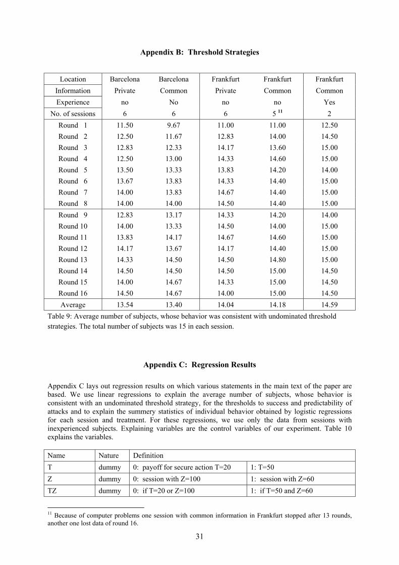
31

Appendix B: Threshold Strategies

Location Barcelona Barcelona Frankfurt Frankfurt Frankfurt Information Private Common Private Common Common Experience no No no no Yes

No. of sessions 6 6 6 5 11 2 Round 1 11.50 9.67 11.00 11.00 12.50 Round 2 12.50 11.67 12.83 14.00 14.50 Round 3 12.83 12.33 14.17 13.60 15.00 Round 4 12.50 13.00 14.33 14.60 15.00 Round 5 13.50 13.33 13.83 14.20 14.00 Round 6 13.67 13.83 14.33 14.40 15.00 Round 7 14.00 13.83 14.67 14.40 15.00 Round 8 14.00 14.00 14.50 14.40 15.00 Round 9 12.83 13.17 14.33 14.20 14.00 Round 10 14.00 13.33 14.50 14.00 15.00 Round 11 13.83 14.17 14.67 14.60 15.00 Round 12 14.17 13.67 14.17 14.40 15.00 Round 13 14.33 14.50 14.50 14.80 15.00 Round 14 14.50 14.50 14.50 15.00 14.50 Round 15 14.00 14.67 14.33 15.00 14.50 Round 16 14.50 14.67 14.00 15.00 14.50 Average 13.54 13.40 14.04 14.18 14.59

Table 9: Average number of subjects, whose behavior was consistent with undominated threshold strategies. The total number of subjects was 15 in each session.

Appendix C: Regression Results Appendix C lays out regression results on which various statements in the main text of the paper are based. We use linear regressions to explain the average number of subjects, whose behavior is consistent with an undominated threshold strategy, for the thresholds to success and predictability of attacks and to explain the summery statistics of individual behavior obtained by logistic regressions for each session and treatment. For these regressions, we use only the data from sessions with inexperienced subjects. Explaining variables are the control variables of our experiment. Table 10 explains the variables. Name Nature Definition T dummy 0: payoff for secure action T=20 1: T=50 Z dummy 0: session with Z=100 1: session with Z=60 TZ dummy 0: if T=20 or Z=100 1: if T=50 and Z=60

11 Because of computer problems one session with common information in Frankfurt stopped after 13 rounds, another one lost data of round 16.

32

Loc(ation) dummy 0: session in Barcelona 1: session in Frankfurt Info(rmation) dummy 0: session with common

information 1: session with private information

Ord(er) dummy 0: session starting with T=50 1: session starting with T=20 TO dummy 0: if Order=0 or T=20 1: if Order=1 and T=50 TS number Average (per session) number of subjects whose behavior is consistent

with an undominated threshold strategy Y* number Mean between highest state up to which all attacks failed and lowest state

from which on all attacks succeeded in all 8 periods. ∆Y* number Distance between the two states defining Y* A number Results from logistic estimation on basis of last four period B number Results from logistic estimation on basis of last four periods Mean number a / b = estimated mean threshold Table 10. Variables used in linear regression.

C.1. Threshold Strategies In all sessions, the number of subjects, whose behavior is consistent with an undominated threshold strategy, tends to increases over time. The average differs across sessions. Regression 1 shows that the information condition is not significant. Regression 2 shows that there may be a significant difference in behavior of subjects from Barcelona and Frankfurt.

Regression 1: TS = β0 + β1 Z + β2 Loc + β3 Info + β4 Ord + u .

Regression 2: TS = β0 + β2 Loc + u .

Explaining variables: estimated β-coefficients (t-values)

No. Data source (Number of

observations) Intercept Z Location Information Order

R2 Adjusted R2

1 All sessions (23)

13.39 (51.43)

0.33 (0.82)

0.50 (1.64)

-0.04 (-0.14)

0.18 (0.69)

0.27 0.11

2 All sessions (23)

13.47 (76.69)

0.63 (2.48)

0.23 0.19

Table 11. Regressions explaining the average number of subjects, whose behavior is consistent with undominated threshold strategies.

C.2. Thresholds to Success Threshold states Y* from which on an attack is likely to occur depend on various of the exogenous conditions.

Regression 3: Y* = γ0 + γ1 T + γ2 Z + γ3 TZ + u .

Regression 4: Y* = γ0 + γ1 T + γ2 Z + γ3 TZ + γ4 Loc + γ5 Info + γ6 Ord + γ7 TO + u .

Regression 5-6: Y* = γ0 + γ1 T + γ2 Z + γ3 TZ + γ4 Loc + γ6 Ord + γ7 TO + u .

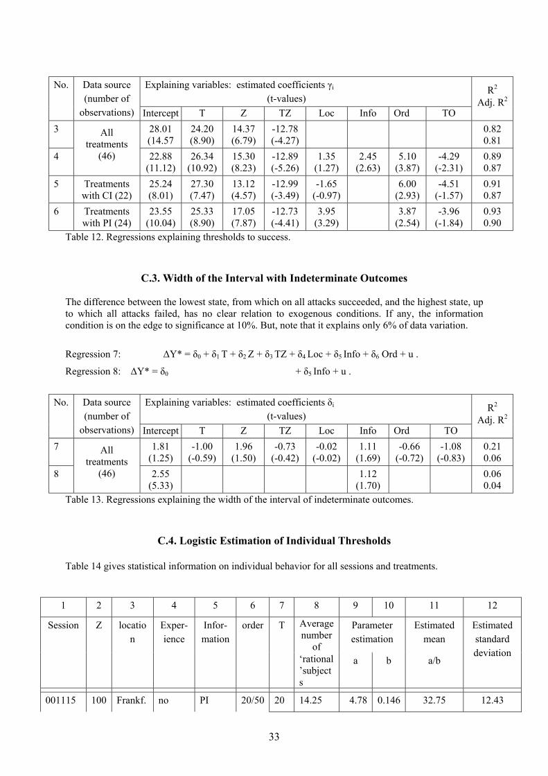
33

Explaining variables: estimated coefficients γi (t-values)

No. Data source (number of

observations) Intercept T Z TZ Loc Info Ord TO

R2 Adj. R2

3 28.01 (14.57

24.20 (8.90)

14.37 (6.79)

-12.78 (-4.27)

0.82 0.81

4

All treatments

(46) 22.88 (11.12)

26.34 (10.92)

15.30 (8.23)

-12.89 (-5.26)

1.35 (1.27)

2.45 (2.63)

5.10 (3.87)

-4.29 (-2.31)

0.89 0.87

5 Treatments with CI (22)

25.24 (8.01)

27.30 (7.47)

13.12 (4.57)

-12.99 (-3.49)

-1.65 (-0.97)

6.00 (2.93)

-4.51 (-1.57)

0.91 0.87

6 Treatments with PI (24)

23.55 (10.04)

25.33 (8.90)

17.05 (7.87)

-12.73 (-4.41)

3.95 (3.29)

3.87 (2.54)

-3.96 (-1.84)

0.93 0.90

Table 12. Regressions explaining thresholds to success.

C.3. Width of the Interval with Indeterminate Outcomes The difference between the lowest state, from which on all attacks succeeded, and the highest state, up to which all attacks failed, has no clear relation to exogenous conditions. If any, the information condition is on the edge to significance at 10%. But, note that it explains only 6% of data variation.

Regression 7: ∆Y* = δ0 + δ1 T + δ2 Z + δ3 TZ + δ4 Loc + δ5 Info + δ6 Ord + u .

Regression 8: ∆Y* = δ0 + δ5 Info + u .

Explaining variables: estimated coefficients δi (t-values)

No. Data source (number of

observations) Intercept T Z TZ Loc Info Ord TO

R2 Adj. R2

7 1.81 (1.25)

-1.00 (-0.59)

1.96 (1.50)

-0.73 (-0.42)

-0.02 (-0.02)

1.11 (1.69)

-0.66 (-0.72)

-1.08 (-0.83)

0.21 0.06

8

All treatments

(46) 2.55 (5.33)

1.12 (1.70)

0.06 0.04

Table 13. Regressions explaining the width of the interval of indeterminate outcomes.

C.4. Logistic Estimation of Individual Thresholds Table 14 gives statistical information on individual behavior for all sessions and treatments.

1 2 3 4 5 6 7 8 9 10 11 12

Session Z location

Exper-ience

Infor-mation

order T Average number

of

Parameter estimation

Estimated mean

‘rational’subjects

a b a/b

Estimated standard deviation

001115 100 Frankf. no PI 20/50 20 14.25 4.78 0.146 32.75 12.43

34

50 14 10.54 0.185 56.91 9.79

001207 100 Frankf. no PI 50/20 50 14.5 10.63 0.199 53.53 9.13

20 14.875 9.35 0.349 26.77 5.19

001206 100 Frankf. no CI 20/50 20 14 8.96 0.271 33.03 6.68

50 14.75 62.18 1.168 53.25 1.55

010131 100 Frankf. no CI 50/20 50 13.625 9.67 0.184 52.66 9.87

20 14.6 9.04 0.462 19.57 3.93 010201 60 Frankf. no PI 20/50 20 13.5 5.43 0.117 46.40 15.50

50 13.625 7.48 0.124 60.21 14.59

010321a 60 Frankf. no PI 50/20 50 12.375 7.67 0.131 58.45 13.82

20 14.125 7.05 0.151 46.62 11.99

010523 60 Frankf. no PI 50/20 50 14 12.75 0.210 60.75 8.64

20 14.875 10.18 0.246 41.42 7.38

010530a 60 Frankf. no PI 20/50 20 13.625 7.42 0.167 44.59 10.89

50 14.75 14.86 0.247 60.10 7.34 010207 60 Frankf. no CI 20/50 20 14.375 8.18 0.212 38.52 8.54

50 14.625 24.74 0.434 56.96 4.18

010321b 60 Frankf. no CI 50/20 50 12.5 7.60 0.166 45.75 10.92

20 14 9.27 0.285 32.57 6.38

010530b 60 Frankf. no CI 50/20 50 14.625 13.19 0.280 47.16 6.49

20 14.875 4.90 0.154 31.90 11.82 0529LN 60 Barcel. no PI 20/50 20 12.375 7.80 0.183 42.72 9.93

50 13 7.79 0.144 54.07 12.60

0530L1 60 Barcel. no PI 50/20 50 13.875 12.62 0.234 54.00 7.76

20 14.5 9.26 0.255 36.28 7.11

0530P3 60 Barcel. no PI 20/50 20 11.375 7.48 0.167 44.77 10.85

50 14.375 13.41 0.262 51.19 6.93

0607L6 60 Barcel. no PI 50/20 50 13.5 9.47 0.173 54.73 10.48

20 14 9.63 0.252 38.25 7.20

0606L8 60 Barcel. no PI 20/50 20 13.75 7.51 0.173 43.48 10.51

50 14.125 12.24 0.238 59.87 7.62

0608LA 60 Barcel. no PI 50/20 50 13.5 13.01 0.229 56.83 7.92

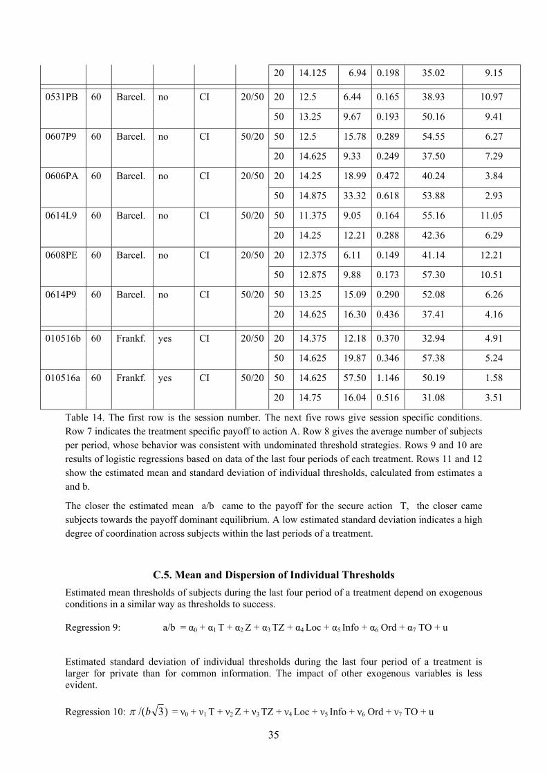
35

20 14.125 6.94 0.198 35.02 9.15 0531PB 60 Barcel. no CI 20/50 20 12.5 6.44 0.165 38.93 10.97

50 13.25 9.67 0.193 50.16 9.41

0607P9 60 Barcel. no CI 50/20 50 12.5 15.78 0.289 54.55 6.27

20 14.625 9.33 0.249 37.50 7.29

0606PA 60 Barcel. no CI 20/50 20 14.25 18.99 0.472 40.24 3.84

50 14.875 33.32 0.618 53.88 2.93

0614L9 60 Barcel. no CI 50/20 50 11.375 9.05 0.164 55.16 11.05

20 14.25 12.21 0.288 42.36 6.29

0608PE 60 Barcel. no CI 20/50 20 12.375 6.11 0.149 41.14 12.21

50 12.875 9.88 0.173 57.30 10.51

0614P9 60 Barcel. no CI 50/20 50 13.25 15.09 0.290 52.08 6.26

20 14.625 16.30 0.436 37.41 4.16 010516b 60 Frankf. yes CI 20/50 20 14.375 12.18 0.370 32.94 4.91

50 14.625 19.87 0.346 57.38 5.24

010516a 60 Frankf. yes CI 50/20 50 14.625 57.50 1.146 50.19 1.58

20 14.75 16.04 0.516 31.08 3.51

Table 14. The first row is the session number. The next five rows give session specific conditions. Row 7 indicates the treatment specific payoff to action A. Row 8 gives the average number of subjects per period, whose behavior was consistent with undominated threshold strategies. Rows 9 and 10 are results of logistic regressions based on data of the last four periods of each treatment. Rows 11 and 12 show the estimated mean and standard deviation of individual thresholds, calculated from estimates a and b.

The closer the estimated mean a/b came to the payoff for the secure action T, the closer came subjects towards the payoff dominant equilibrium. A low estimated standard deviation indicates a high degree of coordination across subjects within the last periods of a treatment.

C.5. Mean and Dispersion of Individual Thresholds Estimated mean thresholds of subjects during the last four period of a treatment depend on exogenous conditions in a similar way as thresholds to success. Regression 9: a/b = α0 + α1 T + α2 Z + α3 TZ + α4 Loc + α5 Info + α6 Ord + α7 TO + u

Estimated standard deviation of individual thresholds during the last four period of a treatment is larger for private than for common information. The impact of other exogenous variables is less evident. Regression 10: )3/(bπ = ν0 + ν1 T + ν2 Z + ν3 TZ + ν4 Loc + ν5 Info + ν6 Ord + ν7 TO + u

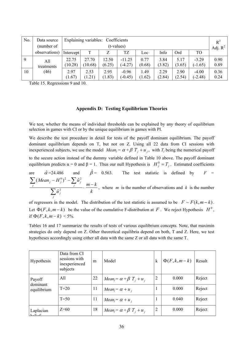
36

Explaining variables: Coefficients (t-values)

No. Data source (number of

observations) Intercept T Z TZ Loc Info Ord TO

R2 Adj. R2

9 22.75 (10.28)

27.70 (10.68)

12.50 (6.25)

-11.25 (-4.27)

0.77 (0.68)

3.84 (3.82)

5.17 (3.65)

-3.29 (-1.65)

0.90 0.89

10

All treatments

(46) 2.97 (1.67)

2.53 (1.21)

2.95 (1.83)

-0.96 (-0.45)

1.49 (1.62)

2.29 (2.84)

2.90 (2.54)

-4.00 (-2.48)

0.36 0.24

Table 15. Regressions 9 and 10.

Appendix D: Testing Equilibrium Theories

We test, whether the means of individual thresholds can be explained by any theory of equilibrium selection in games with CI or by the unique equilibrium in games with PI.

We describe the test procedure in detail for tests of the payoff dominant equilibrium. The payoff dominant equilibrium depends on T, but not on Z. Using all 22 data from CI sessions with inexperienced subjects, we use the model Meanj = α + β jj uT + , with Tj being the numerical payoff

to the secure action instead of the dummy variable defined in Table 10 above. The payoff dominant equilibrium predicts α = 0 and β = 1. Thus our null Hypothesis is jj TH =0 . Estimated coefficients

are α̂ =24.486 and β̂ = 0.563. The test statistic is defined by F =

kkm

u

uHMean

jj

jj

jjj −

⋅−−

∑∑∑

2

220

ˆ

ˆ)(, where m is the number of observations and k is the number

of regressors in the model. The distribution of the test statistic is assumed to be ),(~ kmkFF − . Let ),,( kmkF −Φ be the value of the cumulative F-distribution at F . We reject Hypothesis 0H , if ),,( kmkF −Φ < 5%.

Tables 16 and 17 summarize the results of tests of various equilibrium concepts. Note, that maximin strategies do only depend on Z. Other theoretical equilibria depend on both, T and Z. Here, we test hypotheses accordingly using either all data with the same Z or all data with the same T.

Hypothesis Data from CI sessions with inexperienced subjects

m Model k ),,( kmkF −Φ Result

All 22 Meanj = α + β jj uT + 2 0.000 Reject

T=20 11 Meanj = ju+α 1 0.000 Reject

Payoff dominant equilibrium

T=50 11 Meanj = ju+α 1 0.040 Reject

Laplacian belief

Z=60 18 Meanj = α + β jj uT + 2 0.000 Reject

37

T=20 11 Meanj = α + β jj uZ + 2 0.005 Reject belief equilibrum

T=50 11 Meanj = α + β jj uZ + 2 0.000 Reject

Z=60 18 Meanj = α + β jj uT + 2 0.000 Reject

T=20 11 Meanj = α + β jj uZ + 2 0.004 Reject

Risk dominant equilibrium

T=50 11 Meanj = α + β jj uZ + 2 0.000 Reject

Z=60 18 Meanj = α + β jj uT + 2 0.000 Reject

T=20 11 Meanj = α + β jj uZ + 2 0.000 Reject

‘naïve’ Laplacian belief equilibrium

T=50 11 Meanj = α + β jj uZ + 2 0.068 Accept

Z=60 18 Meanj = α + β jj uT + 2 0.252 Accept

T=20 11 Meanj = α + β jj uZ + 2 0.309 Accept

Best response to belief that others play B with probability 2/3

T=50 11 Meanj = α + β jj uZ + 2 0.542 Accept

Maximin Strategy

All 22 Meanj = α + β jj uZ + 2 0.000 Reject

Table 16. F-tests for selection criteria in sessions with common information.

Hypothesis Data from PI sessions (inexperienced subjects)

m Model k ),,( kmkF −Φ Result

Z=60 20 Meanj = α + β jj uZ + 2 0.000 Reject

T=20 12 Meanj = α + β jj uZ + 2 0.682 Accept

Private information equilibrium

T=50 12 Meanj = α + β jj uZ + 2 0.000 Reject

Table 17. F-tests for equilibrium in sessions with private information.