Hiva Pazira

Lund ObservatoryLund University

Spectroscopy acrossStellar Surfaces

Degree project of 60 higher education credits (for a degree of Master)September 2012

Lund ObservatoryBox 43SE-221 00 LundSweden

2012-EXA69

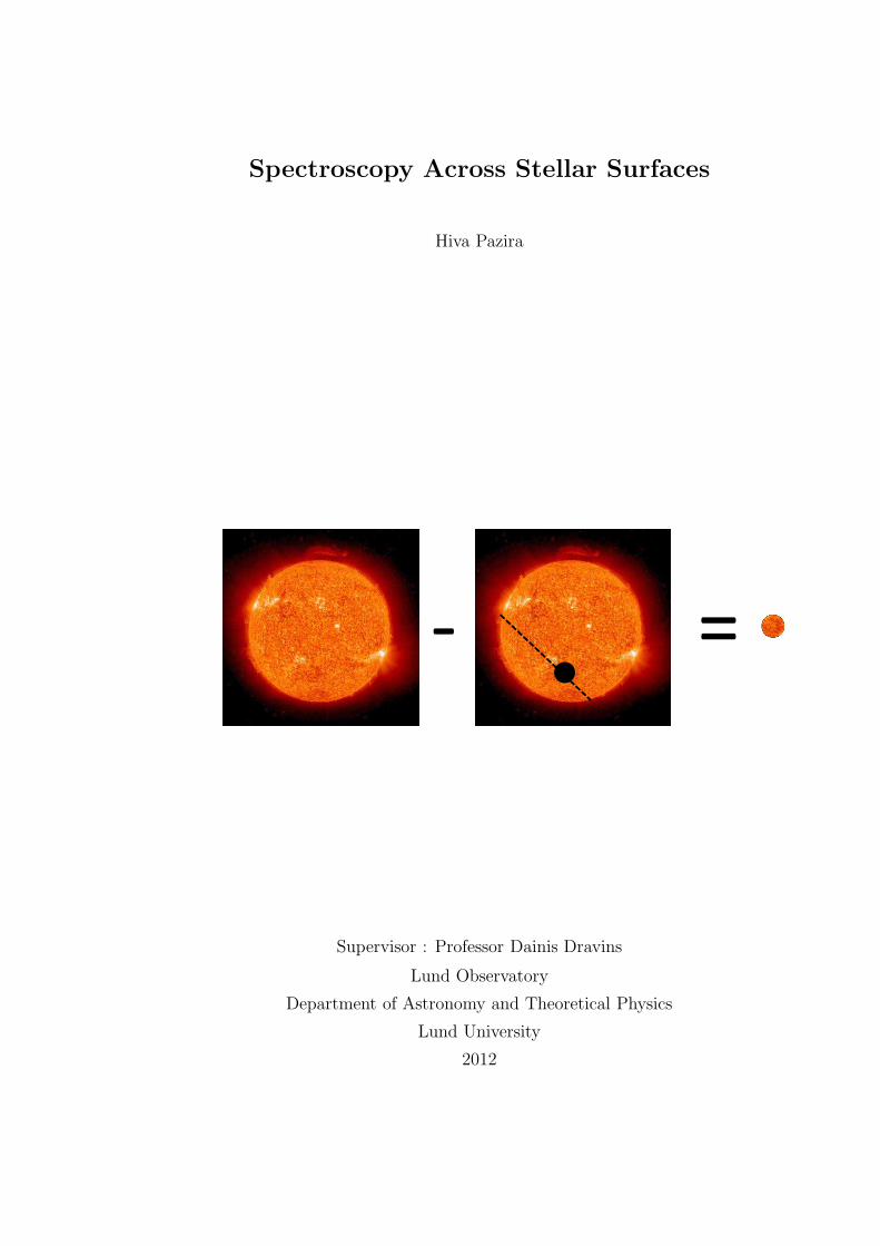
Spectroscopy Across Stellar Surfaces

Hiva Pazira

r =

Supervisor : Professor Dainis Dravins

Lund Observatory

Department of Astronomy and Theoretical Physics

Lund University

2012

Abstract

Stars as we observe them are point source objects and their measured spectra

are integrated over the stellar disk. Since the beginning of stellar spectroscopy, stel-

lar parameters are calculated from these spectra. However recently, simulations of

stellar atmospheres show that it is not possible to determine stellar parameters in a

unique way from disk-averaged data. These 3-dimensional simulations are time de-

pendent and follow the relevant laws of hydrodynamics and radiation. Line profiles

are obtained from physical parameters of each volume element in each time step.

One way to verify these simulations is to resolve the stellar disk and observe

stellar surface structures. The most obvious way of observing would be using an

interferometer or a big telescope. However the existing telescopes and interferometers

are not large enough to resolve the disks of solar-like stars. In this study, another

method is suggested. This method uses planetary transits to measure the spectrum

of a small area on the stellar surface. In this project a set of line profiles from 3D

hydrodynamic models is used to estimated the possibilities of this method.

Also we are examining at what can be observed with one of the next generation

telescopes (E-ELTs) in terms of resolving the disks of giant stars and the shapes of

their line profiles.

ii

Acknowledgements

I intend to express my gratitude to all of those who helped me through, to be

where I am today.

iii

Popularvetenskaplig sammanfattning

Hur skulle stjarnytor se ut om vi kunde observera dem pa nara hall? Vanligtvis

analyseras stjarnor som om de vore sfariska gasbollar, men egentligen ar deras ytor

mer lika ytan i en kastrull med kokande vatten. Detta ”kokande” ger upphov till fina

strukturer over hela stjarnans yta.

Fysiska egenskaper hos en stjarna, som temperatur och kemisk sammansattning,

bestams vanligtvis genom att mata stjarnans spektrum (hur stralningens intensitet

forandras med dess vaglangd), med approximationen att stjarnan ar en slat, sfarisk

gasboll. Stjarnans ytstrukturer forandrar dock spektrat. For att fa exakta resultat

behover man darfor mata dessa parametrar lokalt pa stjarnytan.

Med nuvarande instrument ar det bara mojligt att upplosa ytan pa nagra fa

stjarnor. Dessa stjarnor har radier som ar minst 50 ganger solens, och tillhor en

annan stjarntyp. I en del av detta projekt undersoker vi hur val astronomer kommer

att kunna upplosa ytan pa dessa jattestjarnor i en snar framtid, med hjalp av nasta

generations stora teleskop.

Ungefar 80 % av alla stjarnor har en radie som ar jamforbar med solens, och da

de ligger pa stora avstand fran jorden, ser vi dem som punktkallor. Detta betyder att

vi inte kommer att kunna upplosa dessa stjarnytor och observera deras ytstrukturer

inom en snar framtid. Det finns dock indirekta metoder for att observera dessa

strukturer. I den storre delen av detta arbete diskuteras en sadan metod.

Denna metod ar applicerbar pa stjarnor med planetsystem. Ibland passerar en

planet framfor sin stjarna, under ett tidsintervall som kallas transittiden. Under varje

del av transittiden blockerar planeten ljuset fran en liten del av stjarnytan. Om vi

antar att det genomsnittliga ljuset fran stjarnan ar konstant under transittiden ar

det mojligt att studera strukturer pa stjarnytan som ar sma jamfort med stjarnans

radie. Ljuset fran dessa strukturer blockeras av den passerande planeten, och detta

ljus (och dess spektrum) kan darfor matas som skillnaden i ljusstyrka innan och efter

passagen, och ljuset fran resten av stjarnan under planetens passage.

iv

Contents

Abstract ii

Acknowledgements iii

Popularvetenskaplig sammanfattning iv

1 Introduction 1

1.1 History . . . . . . . . . . . . . . . . . . . . . . . . . . . . . . . . . . . 1

1.2 Light and Spectral lines . . . . . . . . . . . . . . . . . . . . . . . . . 2

1.2.1 Spectral Lines . . . . . . . . . . . . . . . . . . . . . . . . . . . 2

1.2.2 Doppler Effect . . . . . . . . . . . . . . . . . . . . . . . . . . . 3

1.2.3 Thermal Broadening . . . . . . . . . . . . . . . . . . . . . . . 4

1.2.4 Planck Function . . . . . . . . . . . . . . . . . . . . . . . . . . 5

1.3 Stellar Atmospheres . . . . . . . . . . . . . . . . . . . . . . . . . . . . 5

1.4 Surface Effects on Line Profile . . . . . . . . . . . . . . . . . . . . . . 6

1.4.1 Global Effects . . . . . . . . . . . . . . . . . . . . . . . . . . . 7

1.4.1.1 Limb Darkening . . . . . . . . . . . . . . . . . . . . 7

1.4.1.2 Stellar Rotation . . . . . . . . . . . . . . . . . . . . . 9

1.4.2 Local Effects . . . . . . . . . . . . . . . . . . . . . . . . . . . 10

1.4.2.1 Convective Patterns . . . . . . . . . . . . . . . . . . 10

1.4.2.2 Magnetic Fields . . . . . . . . . . . . . . . . . . . . . 12

2 Modeling and Observing Stellar Structures 13

2.1 Stellar Models . . . . . . . . . . . . . . . . . . . . . . . . . . . . . . . 13

2.1.1 Classical Models . . . . . . . . . . . . . . . . . . . . . . . . . 13

v

2.1.2 3-Dimensional Hydrodynamic Models . . . . . . . . . . . . . . 15

2.2 Observing Stellar Surface Structure . . . . . . . . . . . . . . . . . . . 17

2.2.1 Direct Methods . . . . . . . . . . . . . . . . . . . . . . . . . . 17

2.2.1.1 Optical Interferometry . . . . . . . . . . . . . . . . . 18

2.2.1.2 Direct Imaging . . . . . . . . . . . . . . . . . . . . . 19

2.2.2 Indirect Method . . . . . . . . . . . . . . . . . . . . . . . . . . 20

2.2.2.1 Rossiter–McLaughlin Effect . . . . . . . . . . . . . . 20

2.2.2.2 Idea of Indirect method . . . . . . . . . . . . . . . . 22

3 Simulation–Idealized Line Profile 23

3.1 Theory . . . . . . . . . . . . . . . . . . . . . . . . . . . . . . . . . . . 23

3.2 Limb Darkening Effect . . . . . . . . . . . . . . . . . . . . . . . . . . 25

3.3 Stellar Rotation Effect . . . . . . . . . . . . . . . . . . . . . . . . . . 26

3.4 Planet and Displacement Steps . . . . . . . . . . . . . . . . . . . . . 28

3.5 Instrumental Effects and Finite Resolution . . . . . . . . . . . . . . . 33

3.5.1 Spectral Resolution . . . . . . . . . . . . . . . . . . . . . . . . 33

3.5.2 Noise . . . . . . . . . . . . . . . . . . . . . . . . . . . . . . . . 35

4 Simulation–Realistic Line Profile 39

4.1 Initial Conditions . . . . . . . . . . . . . . . . . . . . . . . . . . . . . 39

4.2 Integrated Line Profile . . . . . . . . . . . . . . . . . . . . . . . . . . 41

4.3 Transiting Planet . . . . . . . . . . . . . . . . . . . . . . . . . . . . . 42

4.4 Noise . . . . . . . . . . . . . . . . . . . . . . . . . . . . . . . . . . . . 44

5 Direct Imaging with E-ELT 46

5.1 Theory . . . . . . . . . . . . . . . . . . . . . . . . . . . . . . . . . . . 46

5.2 Simulation of E-ELT Observations . . . . . . . . . . . . . . . . . . . . 49

6 Conclusion 57

Bibliography 59

vi

Chapter 1

Introduction

1.1 History

As we look at the stars in the sky, light is the only parameter that we can measure, by

which we acquire most information that has led to our knowledge about the Universe.

Until the seventeenth century, astronomers were looking at the sky and trying

to measure the intensity of stellar light by naked eye, integrated over all the visible

wavelengths. In 1672 Isaac Newton, passed sunlight through a circular hole into a

prism and a rainbow spectrum appeared on the screen. This event can be considered

as the first spectroscopic experiment in astronomy. With later experiments he real-

ized, by leading all the colors of the spectrum into the same direction, one gets white

light again [16].

In 1802William Hyde Wollaston repeated Newton’s experiment using a slit instead

of a circular hole and he noticed dark lines in the spectrum which he assumed to be

natural boundaries between colors. Later, in 1817 Joseph von Fraunhofer made the

first spectrograph, and not only did he observe the few dark lines that Wollaston had

reported but many hundreds of them [10]. He named the darkest ones from blue to

red alphabetically. Figure 1.1 shows his drawing of solar spectrum that he published

in 1817 [10]. Astronomers still use the same names as Fraunhofer gave to these dark

lines in spectrum [16].

Later in Heidelberg, in 1859, Gustav Kirchhoff and Robert Bunsen discovered that

some of the dark lines are related to chemical elements. For example, the Fraunhofer

1

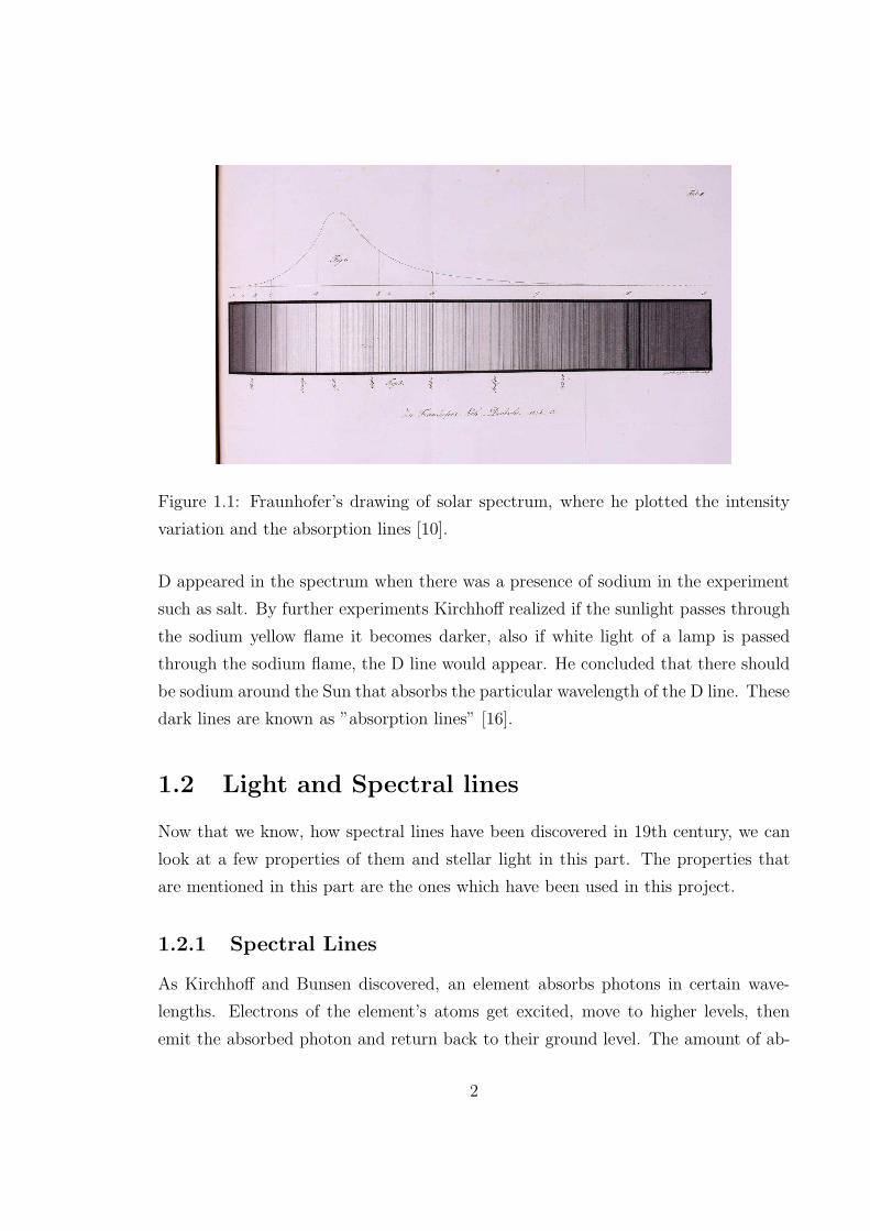
Figure 1.1: Fraunhofer’s drawing of solar spectrum, where he plotted the intensity

variation and the absorption lines [10].

D appeared in the spectrum when there was a presence of sodium in the experiment

such as salt. By further experiments Kirchhoff realized if the sunlight passes through

the sodium yellow flame it becomes darker, also if white light of a lamp is passed

through the sodium flame, the D line would appear. He concluded that there should

be sodium around the Sun that absorbs the particular wavelength of the D line. These

dark lines are known as ”absorption lines” [16].

1.2 Light and Spectral lines

Now that we know, how spectral lines have been discovered in 19th century, we can

look at a few properties of them and stellar light in this part. The properties that

are mentioned in this part are the ones which have been used in this project.

1.2.1 Spectral Lines

As Kirchhoff and Bunsen discovered, an element absorbs photons in certain wave-

lengths. Electrons of the element’s atoms get excited, move to higher levels, then

emit the absorbed photon and return back to their ground level. The amount of ab-

2

sorbed energy is equal to the energy difference between these two levels. An electron

can be excited to different levels and excitations to each level appear as spectral lines.

The energy difference between two levels is a constant value, but as we can see in

Fraunhofer’s drawing, solar spectral lines are not very sharp and they have different

widths. One of the mechanisms that makes the lines wider is the temperature of

the environment. This type of broadening is known as thermal broadening. Before

demonstrating the thermal broadening, there should be an explanation about the

Doppler effect.

1.2.2 Doppler Effect

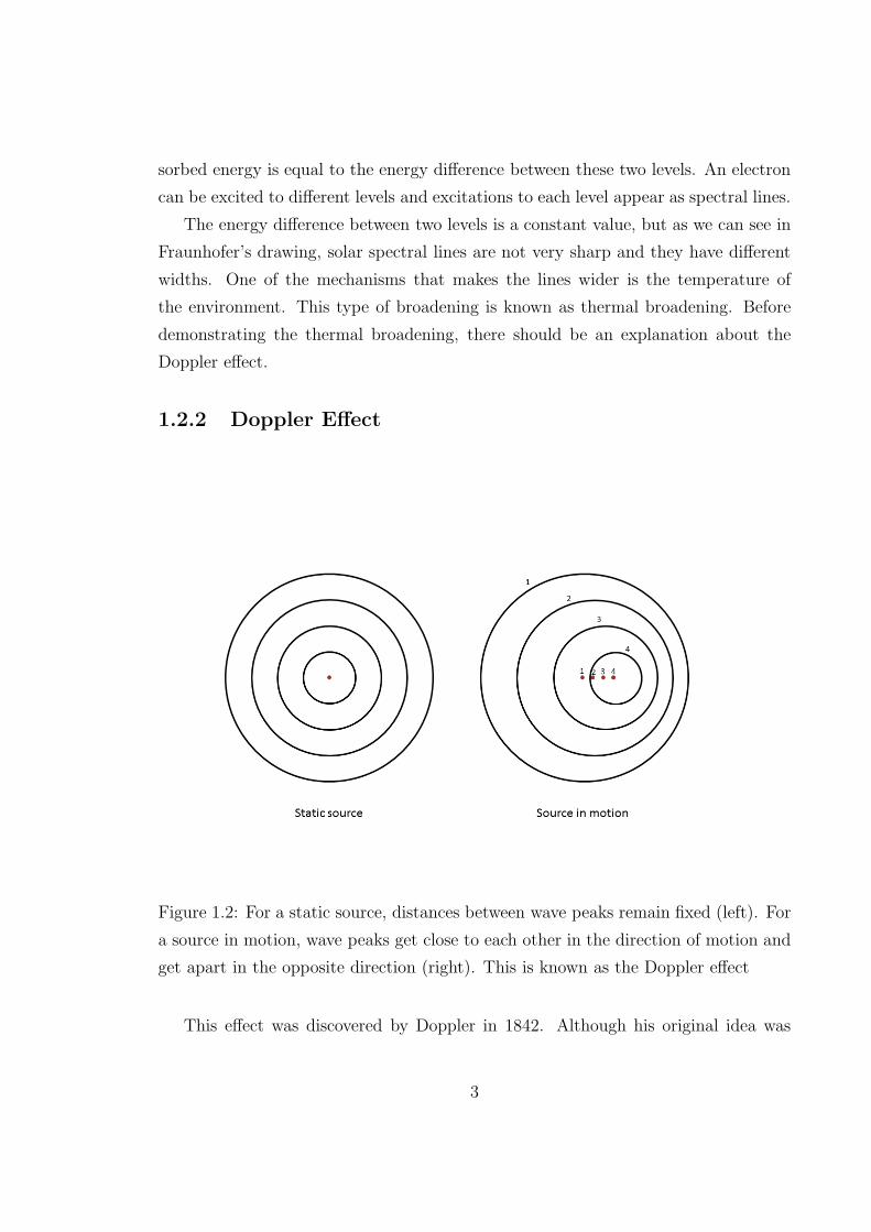
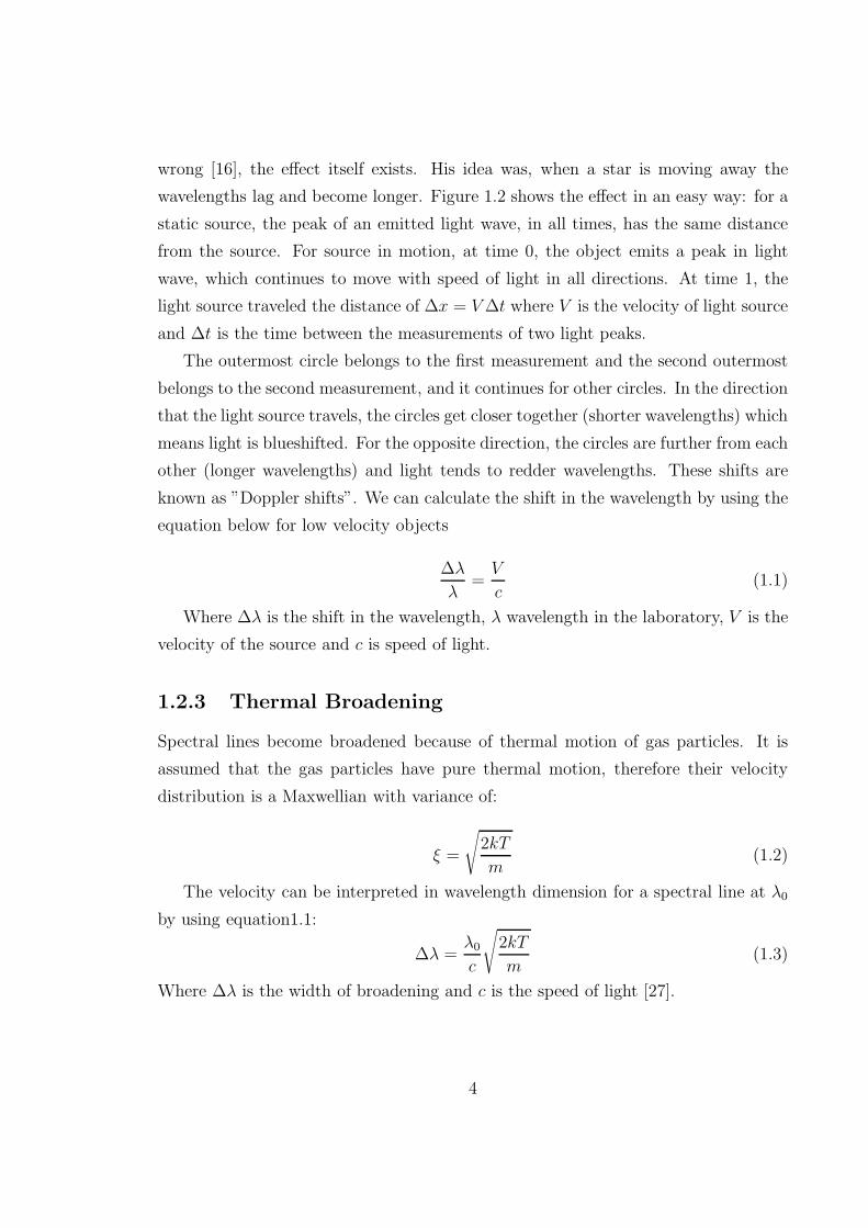
Figure 1.2: For a static source, distances between wave peaks remain fixed (left). For

a source in motion, wave peaks get close to each other in the direction of motion and

get apart in the opposite direction (right). This is known as the Doppler effect

This effect was discovered by Doppler in 1842. Although his original idea was

3

wrong [16], the effect itself exists. His idea was, when a star is moving away the

wavelengths lag and become longer. Figure 1.2 shows the effect in an easy way: for a

static source, the peak of an emitted light wave, in all times, has the same distance

from the source. For source in motion, at time 0, the object emits a peak in light

wave, which continues to move with speed of light in all directions. At time 1, the

light source traveled the distance of ∆x = V∆t where V is the velocity of light source

and ∆t is the time between the measurements of two light peaks.

The outermost circle belongs to the first measurement and the second outermost

belongs to the second measurement, and it continues for other circles. In the direction

that the light source travels, the circles get closer together (shorter wavelengths) which

means light is blueshifted. For the opposite direction, the circles are further from each

other (longer wavelengths) and light tends to redder wavelengths. These shifts are

known as ”Doppler shifts”. We can calculate the shift in the wavelength by using the

equation below for low velocity objects

∆λ

λ=

V

c(1.1)

Where ∆λ is the shift in the wavelength, λ wavelength in the laboratory, V is the

velocity of the source and c is speed of light.

1.2.3 Thermal Broadening

Spectral lines become broadened because of thermal motion of gas particles. It is

assumed that the gas particles have pure thermal motion, therefore their velocity

distribution is a Maxwellian with variance of:

ξ =

√

2kT

m(1.2)

The velocity can be interpreted in wavelength dimension for a spectral line at λ0

by using equation1.1:

∆λ =λ0

c

√

2kT

m(1.3)

Where ∆λ is the width of broadening and c is the speed of light [27].

4

1.2.4 Planck Function

Intensity as a function of wavelength for stars has a shape which is known as black-

body radiation. A black body is an idealized object which absorbs all the electromag-

netic radiation. This property makes the object emit a continuous electromagnetic

spectrum. Hot metals and hot gases are approximately good examples of blackbody

objects. The shape of the intensity function is known as Planck function (top drawing

of Figure 1.1) which depends on the surface temperature of the object. Objects with

higher temperature have higher intensity in all wavelengths and their intensity peak

is in shorter wavelengths.

When the emission source has the shape of the Planck function, the source is in

thermodynamic equilibrium. The source may be in Local Thermodynamic Equilib-

rium (LTE), if the temperature changes at different parts of the source. This changes

the Planck functions in different parts.

1.3 Stellar Atmospheres

We continue this chapter with some information about the stars with low surface

temperature, to explain how the blackbody spectrum is produced in these stars and

how spectral lines appear in the spectrum.

The color of low surface temperature stars is between yellow and red, and their

interior structures differs from stars with high surface temperature. The cores of stars

produce energy by burning hydrogen to helium, via nuclear fusion. This energy is

emitted as high energy photons. Above the core there is a radiative layer where energy

is transported outwards. Since the density is high in the stellar interior, photons are

absorbed and re-emitted or scattered by gas particles, while passing through this

layer. These processes shift the photons all over the electromagnetic spectrum. For

solar-like stars the radiative layer includes the first 70 percent of stellar radius.

The outermost layer in low-temperature stars is a convective zone. Hot, deep

plasma fluids rise outwards, where they release their energy as photons, cool down,

and sink again. Stars with lower temperature have a higher fraction of convective

layer. In very low temperature stars, there is no radiative layer and the whole star

become convective. The uppermost part of the convective layer is where the light

5

that we observe is emitted from, and is merged with the beginning of the stellar

atmosphere. We will discuss the Sun’s atmosphere as an example of these stars,

which can be divided in three layers: photosphere, chromosphere and corona.

The deepest layer of the solar atmosphere is the photosphere. This layer is only

400 km thick, and all that we observe in the Sun and other stars in the optical is

coming from this layer. The opacity in this layer is low enough that the photons

are emitted from the surface. More explanations about the photosphere is given

throughout this study.

The second layer of the solar atmosphere is the chromosphere, ”color sphere”.

With the naked eye, it is only visible during the beginning and the end of total solar

eclipse. It is about 2000 km in radial extent. Unlike the photosphere, temperature

increases between 4400 K to 25000 K and it has emission lines, especially Balmer

series which gives ”rose color” to it [11].

The highest layer of the solar atmosphere is called the corona. It extends to

several million kilometers. The corona is not a sphere around the Sun and especially

when the sun is quiet it looks like streams around the sun [21]. There are emission

lines from FeXVI at 5303 A which means that the temperature is about 2 millionK

[9]. Although it has high temperature, this layer is very dim in optical range and its

brightness is about one million times less than the center of the Sun [28] which is due

to its very low density, about (1011 atomcm3 ). Compared to the photosphere (1023 atom

cm3 ),

and breathing air (1025 atom

cm3 ) this value is very low [11].

1.4 Surface Effects on Line Profile

There are effects that change the characteristics of line profiles such as depth, width

or the continuum level. We can divide these effects into two groups, global and local.

Global effects are the ones that change the shape of spectral line at the stellar surface,

and they can be estimated as a function of position at the disk. The local effects are

the ones that change the shape, locally in the small regions, across the surface.

6

1.4.1 Global Effects

The best-known effect that was discovered in the beginning of stellar spectroscopy

by Cecilia Payne is the dependence of the equivalent width of the spectral lines on

the surface temperature [16]. As also mentioned in part 1.1, the equivalent width

depends on the abundances of the absorbing elements.

The effects that depend on the location of the observer can be written as function

of position at stellar disk. Stellar rotation and limb darkening are the most known

ones.

1.4.1.1 Limb Darkening

This effect changes the continuum level of the intensity across the stellar disk. Figure

1.3 shows the variation in continuum level. In both regions A and B, we are looking

through the stellar atmosphere and we can only look into one unit of optical depth.

In region A we are looking at the deeper layer of the Sun’s photosphere which has

higher temperature compared to B, where we are looking at an upper layer. Higher

temperature appears as higher intensity.

As we observe the stellar surface from the center to limb we are scanning from

deeper layers with higher temperature and higher intensity, to the higher layers in

the atmosphere with lower temperature and lower intensity. The length of a unit of

optical depth is different for different wavelengths, as we can see in Figure 1.4 the

effect of limb darkening in different optical wavelengths [13].

As mentioned in section 1.3, the temperature increases in higher layer of the

atmosphere, therefore for the UV and X-ray regions instead of limb darkening, there

would be limb brightening.

One function to describe the variation of continuum intensity across stellar disk is

a linear function dependent on the projected distance from the center. The viewing

angle θ is the angle between the observer and the normal vector of a position at stellar

sphere, and µ is:

µ = cos(θ) (1.4)

7

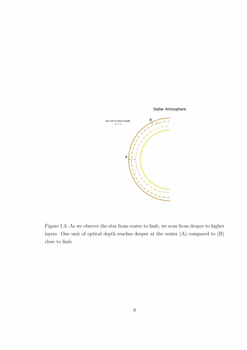
Figure 1.3: As we observe the star from center to limb, we scan from deeper to higher

layers. One unit of optical depth reaches deeper at the center (A) compared to (B)

close to limb

8

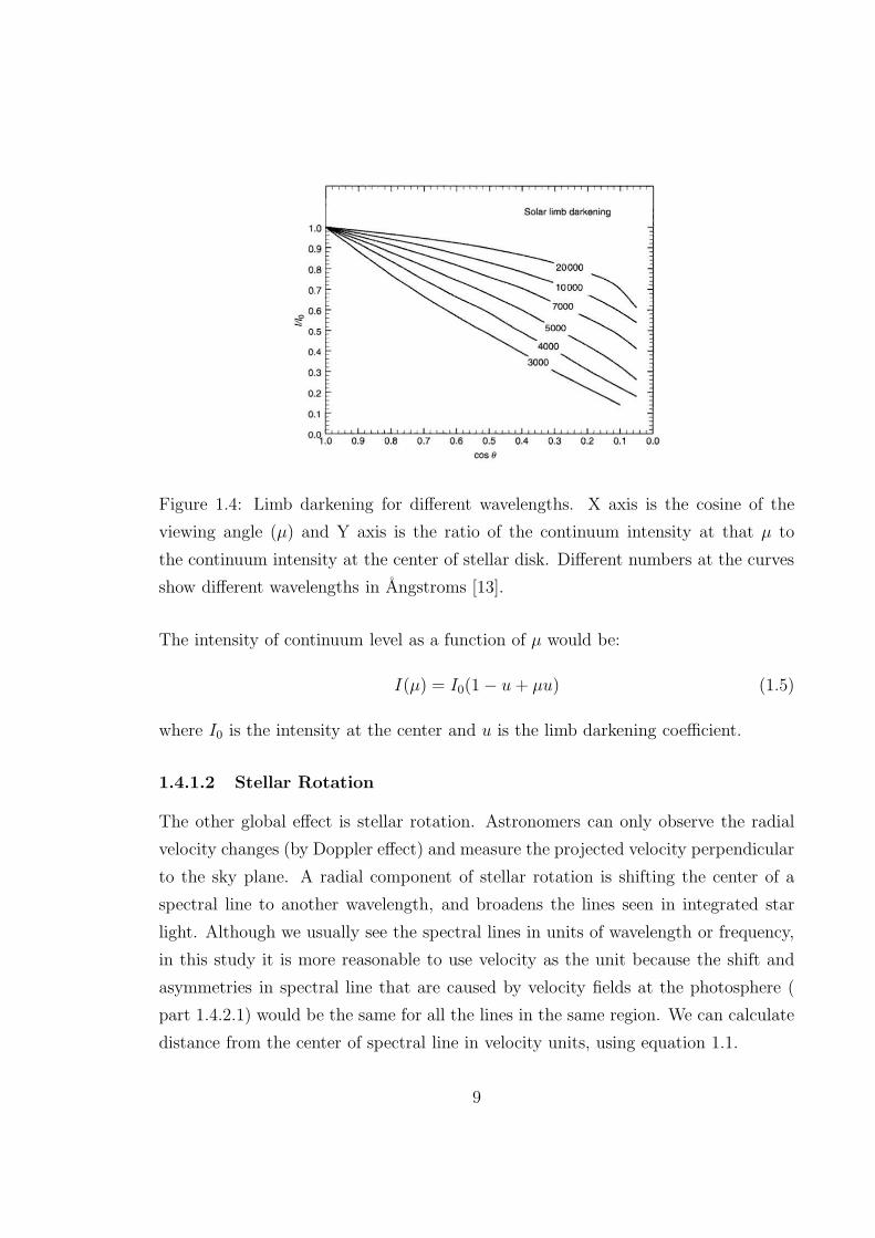
Figure 1.4: Limb darkening for different wavelengths. X axis is the cosine of the

viewing angle (µ) and Y axis is the ratio of the continuum intensity at that µ to

the continuum intensity at the center of stellar disk. Different numbers at the curves

show different wavelengths in Angstroms [13].

The intensity of continuum level as a function of µ would be:

I(µ) = I0(1− u+ µu) (1.5)

where I0 is the intensity at the center and u is the limb darkening coefficient.

1.4.1.2 Stellar Rotation

The other global effect is stellar rotation. Astronomers can only observe the radial

velocity changes (by Doppler effect) and measure the projected velocity perpendicular

to the sky plane. A radial component of stellar rotation is shifting the center of a

spectral line to another wavelength, and broadens the lines seen in integrated star

light. Although we usually see the spectral lines in units of wavelength or frequency,

in this study it is more reasonable to use velocity as the unit because the shift and

asymmetries in spectral line that are caused by velocity fields at the photosphere (

part 1.4.2.1) would be the same for all the lines in the same region. We can calculate

distance from the center of spectral line in velocity units, using equation 1.1.

9

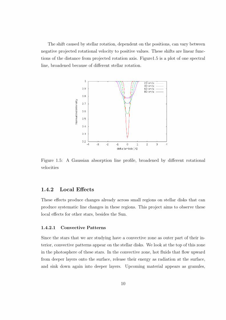
The shift caused by stellar rotation, dependent on the positions, can vary between

negative projected rotational velocity to positive values. These shifts are linear func-

tions of the distance from projected rotation axis. Figure1.5 is a plot of one spectral

line, broadened because of different stellar rotation.

Figure 1.5: A Gaussian absorption line profile, broadened by different rotational

velocities

1.4.2 Local Effects

These effects produce changes already across small regions on stellar disks that can

produce systematic line changes in these regions. This project aims to observe these

local effects for other stars, besides the Sun.

1.4.2.1 Convective Patterns

Since the stars that we are studying have a convective zone as outer part of their in-

terior, convective patterns appear on the stellar disks. We look at the top of this zone

in the photosphere of these stars. In the convective zone, hot fluids that flow upward

from deeper layers onto the surface, release their energy as radiation at the surface,

and sink down again into deeper layers. Upcoming material appears as granules,

10

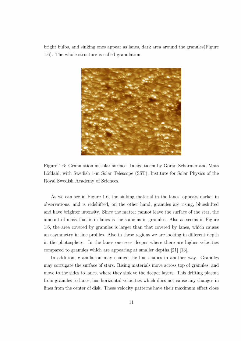
bright bulbs, and sinking ones appear as lanes, dark area around the granules(Figure

1.6). The whole structure is called granulation.

Figure 1.6: Granulation at solar surface. Image taken by Goran Scharmer and Mats

Lofdahl, with Swedish 1-m Solar Telescope (SST), Institute for Solar Physics of the

Royal Swedish Academy of Sciences.

As we can see in Figure 1.6, the sinking material in the lanes, appears darker in

observations, and is redshifted, on the other hand, granules are rising, blueshifted

and have brighter intensity. Since the matter cannot leave the surface of the star, the

amount of mass that is in lanes is the same as in granules. Also as seems in Figure

1.6, the area covered by granules is larger than that covered by lanes, which causes

an asymmetry in line profiles. Also in these regions we are looking in different depth

in the photosphere. In the lanes one sees deeper where there are higher velocities

compared to granules which are appearing at smaller depths [21] [13].

In addition, granulation may change the line shapes in another way. Granules

may corrugate the surface of stars. Rising materials move across top of granules, and

move to the sides to lanes, where they sink to the deeper layers. This drifting plasma

from granules to lanes, has horizontal velocities which does not cause any changes in

lines from the center of disk. These velocity patterns have their maximum effect close

11

to the limb where horizontal velocities are in the direction of the line of sight. This

phenomenon makes the lines broader [8] [7].

1.4.2.2 Magnetic Fields

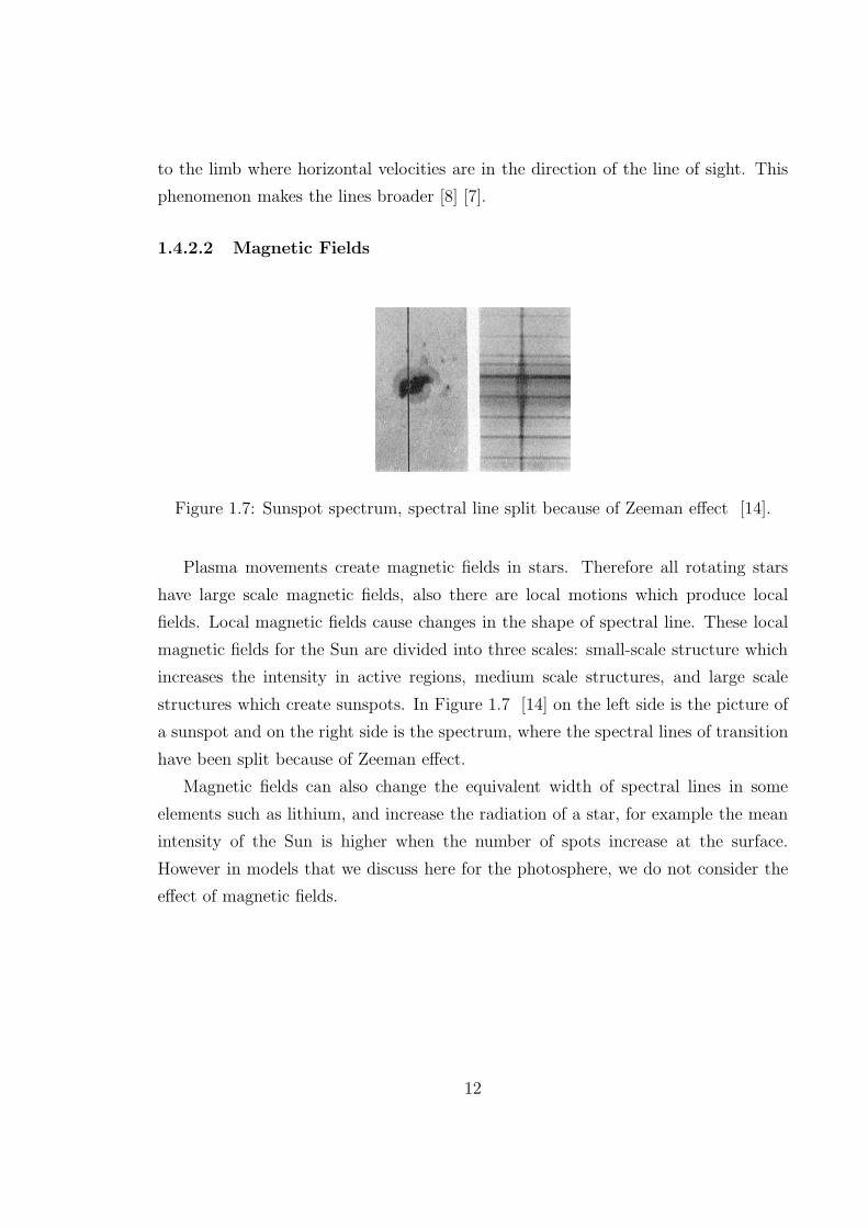
Figure 1.7: Sunspot spectrum, spectral line split because of Zeeman effect [14].

Plasma movements create magnetic fields in stars. Therefore all rotating stars

have large scale magnetic fields, also there are local motions which produce local

fields. Local magnetic fields cause changes in the shape of spectral line. These local

magnetic fields for the Sun are divided into three scales: small-scale structure which

increases the intensity in active regions, medium scale structures, and large scale

structures which create sunspots. In Figure 1.7 [14] on the left side is the picture of

a sunspot and on the right side is the spectrum, where the spectral lines of transition

have been split because of Zeeman effect.

Magnetic fields can also change the equivalent width of spectral lines in some

elements such as lithium, and increase the radiation of a star, for example the mean

intensity of the Sun is higher when the number of spots increase at the surface.

However in models that we discuss here for the photosphere, we do not consider the

effect of magnetic fields.

12

Chapter 2

Modeling and Observing Stellar

Structures

2.1 Stellar Models

Astronomers use spectral lines to measure stellar parameters such as temperature,

abundance of elements in stars, rotational velocity of star, velocity fields in the stellar

photosphere, surface gravity, etc. All of these parameters can be considered indepen-

dent from each other which makes it difficult to estimate stellar parameters. Therefore

there are simplified models of stellar atmospheres which simulate the stellar spectrum

based on wide range of mentioned parameters. By comparing the simulated spectrum

with the observed one, we will be able to measure stellar parameters. Here is a brief

explanation about stellar atmosphere models.

2.1.1 Classical Models

The first models of stellar atmospheres were one-dimensional, hydrostatic models. In

these models it is assumed that all the physical parameters are functions of one spatial

parameter, radial distance from the center, known as the plane parallel geometry.

Structures on the stellar disk, such as granulation and the effect of the magnetic fields,

are not taken into account in these models. It is also assumed that the acceleration

of gas particles in the photosphere are smaller than the surface gravity of the star.

The changes in velocity fields are averaged by turbulence parameters.

13

Modeling the stellar photosphere with these assumptions started in the beginning

of stellar spectroscopy. In 1928, Rosseland [25], used the term ”turbulence” for the

velocity fields in the photosphere. Depending on the size of the turbulence cells, there

are two different types, micro- and macroturbulence. The optical depth is used to

distinguish the turbulence type; any velocity field smaller than one unit of optical

depth is called micro and those larger are called macroturbulence. The turbulence

does not change the dynamic properties of stellar atmospheres, like temperature or

pressure. It only affects kinematics like changing the velocity of the gas particles. [13]

Microturbulence is used when velocity fields are smaller than the optical depth in

the atmosphere. It is assumed that microturbulence is isotropic in stars. The esti-

mation of its mean velocity fields is about 1− 2kms−1. Since microturbulence eddies

are small, micro turbulence velocity can be included in the velocity of particles in the

photosphere which will lead to an increase the thermal broadening in spectral lines.

Thus the spectral lines become broader and the line shape would have a Gaussian

distribution. [13]

The macroturbulence cells are larger than a unit of optical depth which means

that photons stay in a macroturbulence cell from the time of their creation until the

emission from the stellar surface. These velocity fields are related to the position at

stellar disk and can be divided into tangential and radial velocities. The value of

tangential velocity depends on x coordinate and the value of radial velocity depends

on the y coordinate on the stellar disk. If we assume the stellar disk as a disk with

radius 1, the x positions are the cosine of the polar angles and the y positions are

the sine of polar angle of the point on the disk in the polar coordinate system. Since

spectral lines are integrated over the stellar disk, the effect of tangential and radial

velocity of macroturbulence on lines are the same, thus they have the same function

and the same mean velocity. The shape of line profile after considering the effect of

macroturbulence will have a sharper depth with larger wings. [13]

It is easier to estimate the turbulence parameters for low temperature stars, be-

cause they have deeper convective layers; thus the turbulence has higher mean values

in these stars. Also rotational velocities of hot stars are higher which will lead to

some difficulties in estimating of stellar parameters. [13]

Although solar observations from 1950s showed that turbulence does not exist in

14

the sense that it was presumed in the photosphere models, the classical models are

still the most useful tools to measure stellar parameters via spectroscopy. They have

been produced for large grids of stellar parameters and they cover many physical

processes in detail.

Currently astronomers are producing 3-dimensional models of photospheres to get

more accurate and precise estimations of stellar parameters.

2.1.2 3-Dimensional Hydrodynamic Models

As it appears in the name of these models, stellar parameters are a function of three

dimensional coordinates. These models are also time dependent and thus the shape

of simulated spectral lines would be different in each time step.

In these models, the only free parameters are effective temperature, chemical

abundance and surface gravity [6]. Since these models have a small number of free

parameters and they are 3D, they can predict the stellar atmospheric parameters

from the chromosphere to convective layers below the photosphere [31], while 1D

simulations only predict the photosphere.

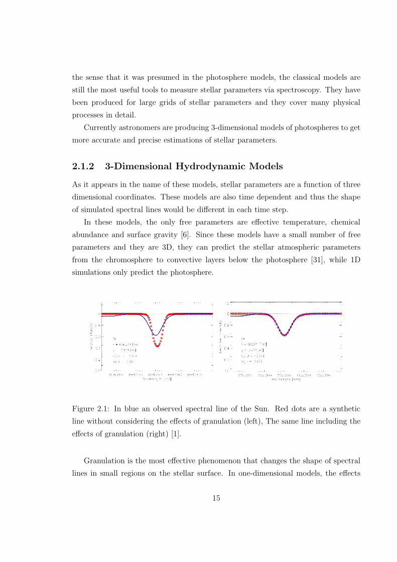
Figure 2.1: In blue an observed spectral line of the Sun. Red dots are a synthetic

line without considering the effects of granulation (left), The same line including the

effects of granulation (right) [1].

Granulation is the most effective phenomenon that changes the shape of spectral

lines in small regions on the stellar surface. In one-dimensional models, the effects

15

of granulations is not considered. Figure 2.1(left), shows an observed spectral line of

the solar flux atlas in blue (solid line) and the same line profile, is simulated without

considering the effects of granulation in red dots. Figure 2.1 (right), show the same

spectral line including the granulation effects (red dots) [1].

These simulations are made in LTE which is when the source of emission has the

shape of a Planck function, but in some cases the effect of non-LTE is also considered.

Later line profiles can extracted from the results of these simulations.

There are two ways to simulate stellar surfaces. In one, a cubic volume (grid) of

stellar surfaces is simulated. The length of each side of this grid might be perhaps 3

granules. In the other one, the whole star is simulated. This model is used for giants

and super giants where the size of granules is comparable to the radius of the star. In

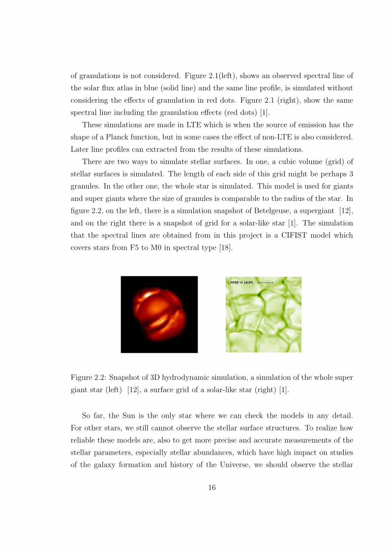
figure 2.2, on the left, there is a simulation snapshot of Betelgeuse, a supergiant [12],

and on the right there is a snapshot of grid for a solar-like star [1]. The simulation

that the spectral lines are obtained from in this project is a CIFIST model which

covers stars from F5 to M0 in spectral type [18].

Figure 2.2: Snapshot of 3D hydrodynamic simulation, a simulation of the whole super

giant star (left) [12], a surface grid of a solar-like star (right) [1].

So far, the Sun is the only star where we can check the models in any detail.

For other stars, we still cannot observe the stellar surface structures. To realize how

reliable these models are, also to get more precise and accurate measurements of the

stellar parameters, especially stellar abundances, which have high impact on studies

of the galaxy formation and history of the Universe, we should observe the stellar

16

structure with different methods.

In the rest of this chapter, we are looking at the goal of this project which is

discussing the methods and their limitation, to observe stellar surface structures with

current instruments, and what we can achieve in near future.

2.2 Observing Stellar Surface Structure

Observing stellar surfaces can be carried out in two ways, resolving a stellar disk

directly and take the spectrum of part of stellar surfaces, which is called ”direct

method”. Although one may use another object in the sky to isolate the spectrum of

the parts that we want to observe; this is called ”indirect method”.

2.2.1 Direct Methods

In direct methods, the stellar disk is resolved and stellar surface structures such as

convective features and big spots can be observed in the optical region of the spectrum.

In this method, we can use an array of small telescopes as an interferometer or we

can use a very large telescope.

The spatial resolution that can be achieved by telescopes is not infinite and it is

limited by the diameter of the telescope mirror or in the case of an interferometer,

the largest distance between telescopes, the baseline.

As soon as a series of plane wavefronts have encounters with a mirror or a lens

in telescopes, their shape changes into spherical wavefronts. Thus in the focal plane

we will see diffraction patterns. The size of this diffraction pattern is dependent on

the size of the mirror or the baseline. A point source object would appear as a disk,

surrounded by rings.

The smallest angular distance between two point sources that can be resolved with

telescopes is known as the diffraction limit which is 0.9 times the half-size of a point

source object in the focal plane. The angular size of this limit can be calculated by:

α = 2.5× 105λ

D(2.1)

Where α is the resolution in arcsec, λ is the wavelength and D is the diameter of

the telescope mirror, or the baseline which must be in the same units as the wave-

17

length. This means that the resolution is higher if we observe in shorter wavelengths

or use bigger telescopes.

We can reach the diffraction limit of the telescope in resolving objects when the

telescopes are outside the Earth’s atmosphere or if the effects of atmosphere are

removed by using Adaptive Optics (AO).

To use the direct method to spatially resolve the stellar disk is not a new idea.

The first detection was at Mount Wilson observatory by Michelson and Pease in

1921 [20]. In this observation the disk of Betelgeuse which is about 50 mas was

resolved. The idea was to use a small telescope parallel to the main telescope, serving

as an interferometer. The small telescope increases the baseline for the interferometer.

Since then, less than a hundred stars have had their angular disks size measured using

interferometry or by taking images with large telescopes.

2.2.1.1 Optical Interferometry

Using optical interferometers improves the diffraction limit, but it also has its techni-

cal difficulties. Currently, Center for High Angular Resolution Astronomy (CHARA)

is the largest optical interferometer with 350 m baseline and 6 Telescopes [24]. The

angular diameters of 74 stars with different spectral types have been measured using

this array [2].

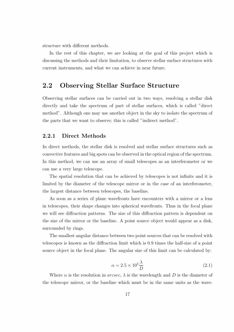
To show an example of detecting surface structures with optical interferometers,

the picture of Betelgeuse taken by Cambridge Optical Aperture Synthesis Telescope

(COAST) and the William Herschel Telescope (WHT), at three wavelengths, from

left to right in 700 nm, 905 nm and 1290 nm is shown in figure 2.3 [32]. Surface

structures on the disk can be detected in the left and the middle figures.

Another array is Magdalena Ridge Observatory Interferometer which is expected

to take the first light in the near future, with 6 telescopes and in its final phase will

have a baseline of about 13 km with 10 telescopes. [5]

This project investigates the two other methods that are explained in the rest of

this chapter.

18

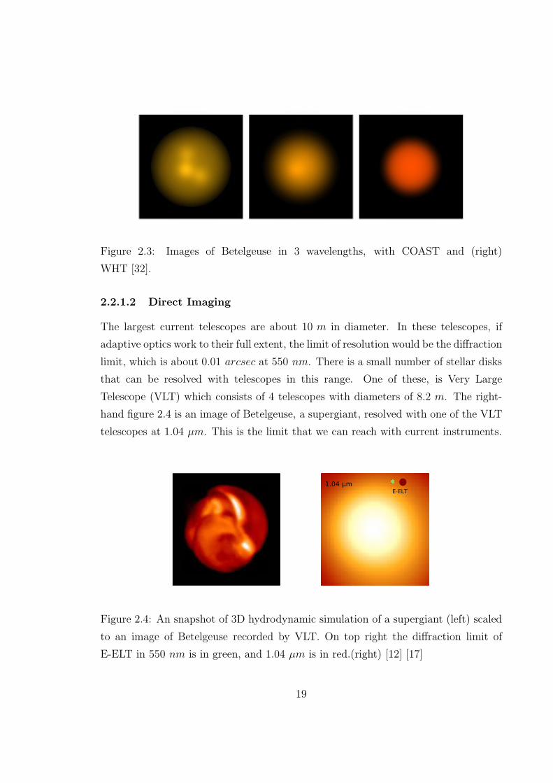
Figure 2.3: Images of Betelgeuse in 3 wavelengths, with COAST and (right)

WHT [32].

2.2.1.2 Direct Imaging

The largest current telescopes are about 10 m in diameter. In these telescopes, if

adaptive optics work to their full extent, the limit of resolution would be the diffraction

limit, which is about 0.01 arcsec at 550 nm. There is a small number of stellar disks

that can be resolved with telescopes in this range. One of these, is Very Large

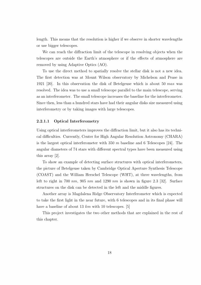
Telescope (VLT) which consists of 4 telescopes with diameters of 8.2 m. The right-

hand figure 2.4 is an image of Betelgeuse, a supergiant, resolved with one of the VLT

telescopes at 1.04 µm. This is the limit that we can reach with current instruments.

Figure 2.4: An snapshot of 3D hydrodynamic simulation of a supergiant (left) scaled

to an image of Betelgeuse recorded by VLT. On top right the diffraction limit of

E-ELT in 550 nm is in green, and 1.04 µm is in red.(right) [12] [17]

19

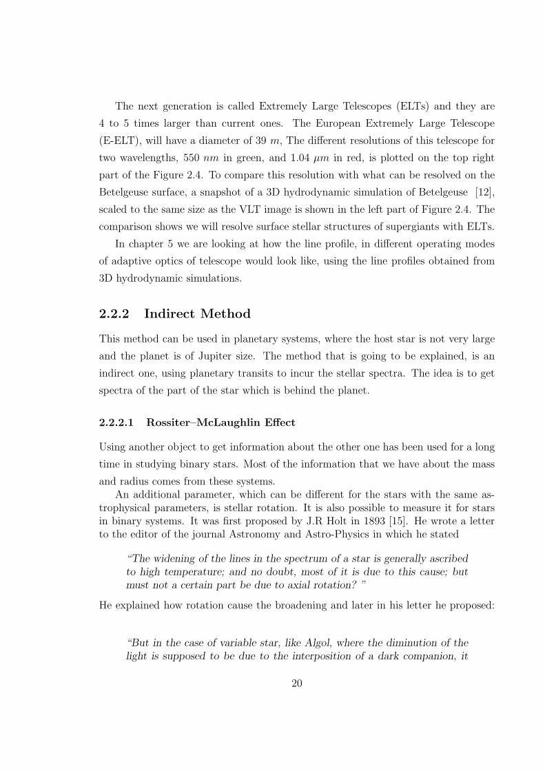
The next generation is called Extremely Large Telescopes (ELTs) and they are

4 to 5 times larger than current ones. The European Extremely Large Telescope

(E-ELT), will have a diameter of 39 m, The different resolutions of this telescope for

two wavelengths, 550 nm in green, and 1.04 µm in red, is plotted on the top right

part of the Figure 2.4. To compare this resolution with what can be resolved on the

Betelgeuse surface, a snapshot of a 3D hydrodynamic simulation of Betelgeuse [12],

scaled to the same size as the VLT image is shown in the left part of Figure 2.4. The

comparison shows we will resolve surface stellar structures of supergiants with ELTs.

In chapter 5 we are looking at how the line profile, in different operating modes

of adaptive optics of telescope would look like, using the line profiles obtained from

3D hydrodynamic simulations.

2.2.2 Indirect Method

This method can be used in planetary systems, where the host star is not very large

and the planet is of Jupiter size. The method that is going to be explained, is an

indirect one, using planetary transits to incur the stellar spectra. The idea is to get

spectra of the part of the star which is behind the planet.

2.2.2.1 Rossiter–McLaughlin Effect

Using another object to get information about the other one has been used for a long

time in studying binary stars. Most of the information that we have about the mass

and radius comes from these systems.An additional parameter, which can be different for the stars with the same as-

trophysical parameters, is stellar rotation. It is also possible to measure it for starsin binary systems. It was first proposed by J.R Holt in 1893 [15]. He wrote a letterto the editor of the journal Astronomy and Astro-Physics in which he stated

“The widening of the lines in the spectrum of a star is generally ascribed

to high temperature; and no doubt, most of it is due to this cause; but

must not a certain part be due to axial rotation? ”

He explained how rotation cause the broadening and later in his letter he proposed:

“But in the case of variable star, like Algol, where the diminution of the

light is supposed to be due to the interposition of a dark companion, it

20

seems to me that there ought to be a spectroscope difference between

the light at the commencement of the minimum phase, and that of the

end, inasmuch as different portions of the edge would be obscured. In

fact, during the progress of the partial eclipse, there should be a shift in

position of the line. ”

This effect is known as Rossiter-McLaughlin effect [26] [19]. They discovered

this effect separately in 1924 and published it in the Astrophysical Journal. As

Holt mentioned, during the minima in eclipsing binaries, one star covers the other.

Assuming that the orbits and stellar rotations have the same directions, during the

first half of the first minimum, the dimmer star covers part of brighter star. This part

is moving towards us and in the second half of the minimum, it covers the part which

is moving away from us. In the first part of the minimum it blocks the blue shifted

part which appears as red shift (lack of blue shift) in spectrum and in the second part

it blocks the redshifted part which in integrated starlight appears as the blue shift.

In the second minimum, the brighter star covers the dimmer one and if the dimmer

object is bright enough, we can detect the effect for the dimmer star as well.

This effect was observed by Queloz et.al. in 2000 for the HD209458 planetary

system [22]. However in planetary transits, the rotational axis of the orbit is not

always the same as the stellar rotation axis. From spectroscopic data with detection

of Rossiter-McLaughlin effect and transit data (photometry), it is possible to deduce

a lot of information about the host star and the planet. But that is not our aim

for this project because, as said before, the aim is to get spectral data from parts of

stellar surfaces.

21

2.2.2.2 Idea of Indirect method

r =

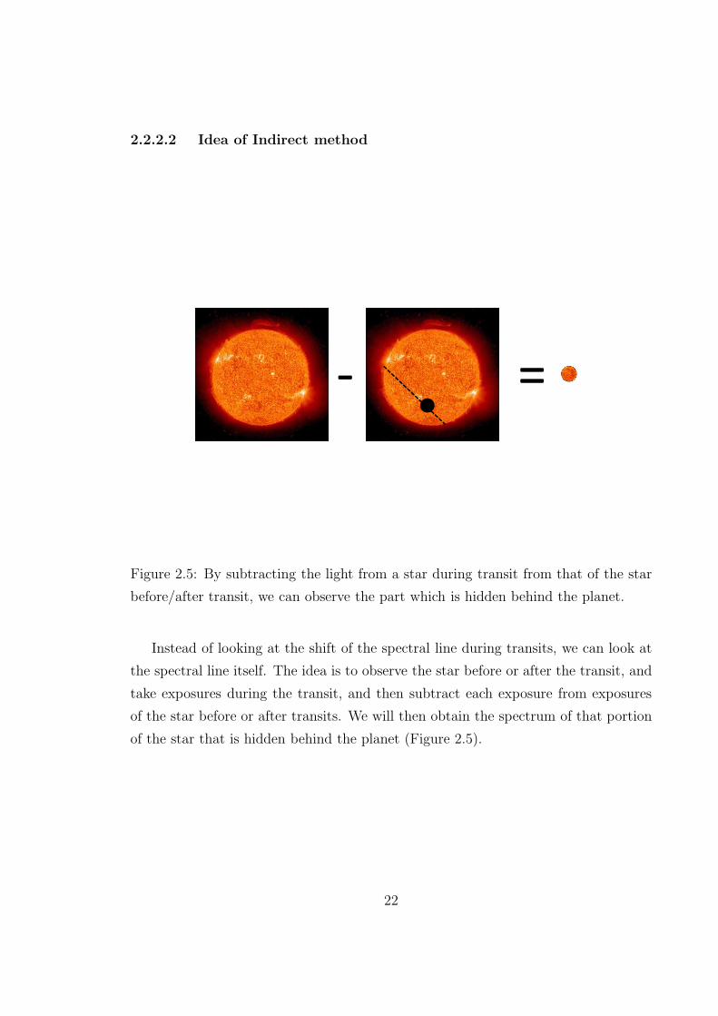
Figure 2.5: By subtracting the light from a star during transit from that of the star

before/after transit, we can observe the part which is hidden behind the planet.

Instead of looking at the shift of the spectral line during transits, we can look at

the spectral line itself. The idea is to observe the star before or after the transit, and

take exposures during the transit, and then subtract each exposure from exposures

of the star before or after transits. We will then obtain the spectrum of that portion

of the star that is hidden behind the planet (Figure 2.5).

22

Chapter 3

Simulation–Idealized Line Profile

3.1 Theory

As mentioned in previous chapter, we are going to simulate the spectrum of a part of

a stellar disk, hidden behind a planet during a transit. In this section, the simulation

method is elaborated. These simulations are estimates of what we expect to observe

with new instruments and technologies in the near future. The simulations were

coded and run in MATLAB.

In order to approximate the spectrum of a part of the stellar surface, we need to

generate spectral line profiles for a sufficient number of positions of a stellar disk.

The first step is to divide the stellar surface into segments, Figure 3.1 (right).

These segments will be called pixels. Using the polar coordinate system is the most

reasonable way of dividing the stellar disk into segments because the segments will

be only a function of the radial coordinate and independent of angular coordinate.

The space between the center and the limb is divided into 30 rings. The number

of rings is in principle arbitrary. 30 is a small number and it does not require a lot

of simulation time. However it is not too small, so that we would miss changes in

the line profiles. The shift of spectral lines between two adjacent rings should be

smaller than the spectral resolution of the spectrograph. Then each ring is covered

by a number of segments (pixels). The center of each pixel is located on a ring and

its radius is half of the distance of two adjacent rings.

Figure 3.1 (left) demonstrates how to find the maximum number of the pixels

23

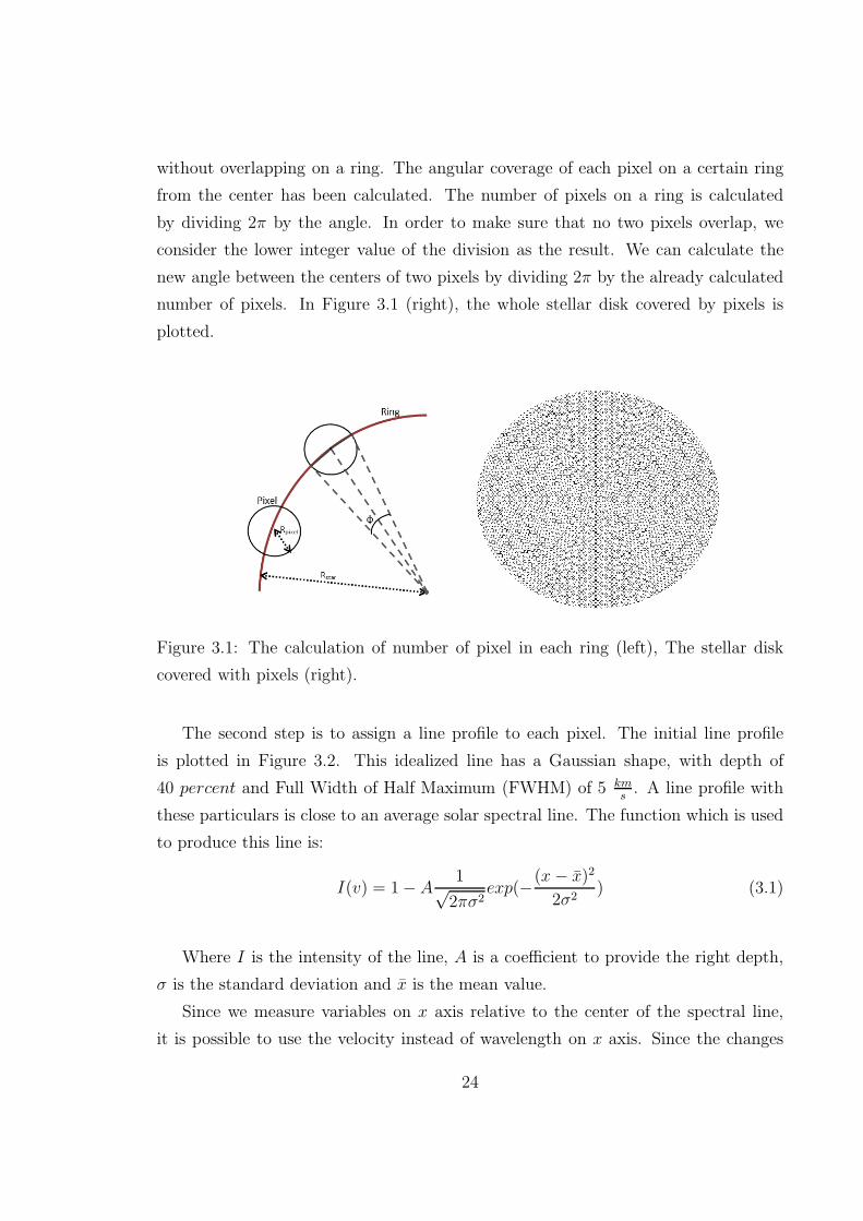
without overlapping on a ring. The angular coverage of each pixel on a certain ring

from the center has been calculated. The number of pixels on a ring is calculated

by dividing 2π by the angle. In order to make sure that no two pixels overlap, we

consider the lower integer value of the division as the result. We can calculate the

new angle between the centers of two pixels by dividing 2π by the already calculated

number of pixels. In Figure 3.1 (right), the whole stellar disk covered by pixels is

plotted.

Figure 3.1: The calculation of number of pixel in each ring (left), The stellar disk

covered with pixels (right).

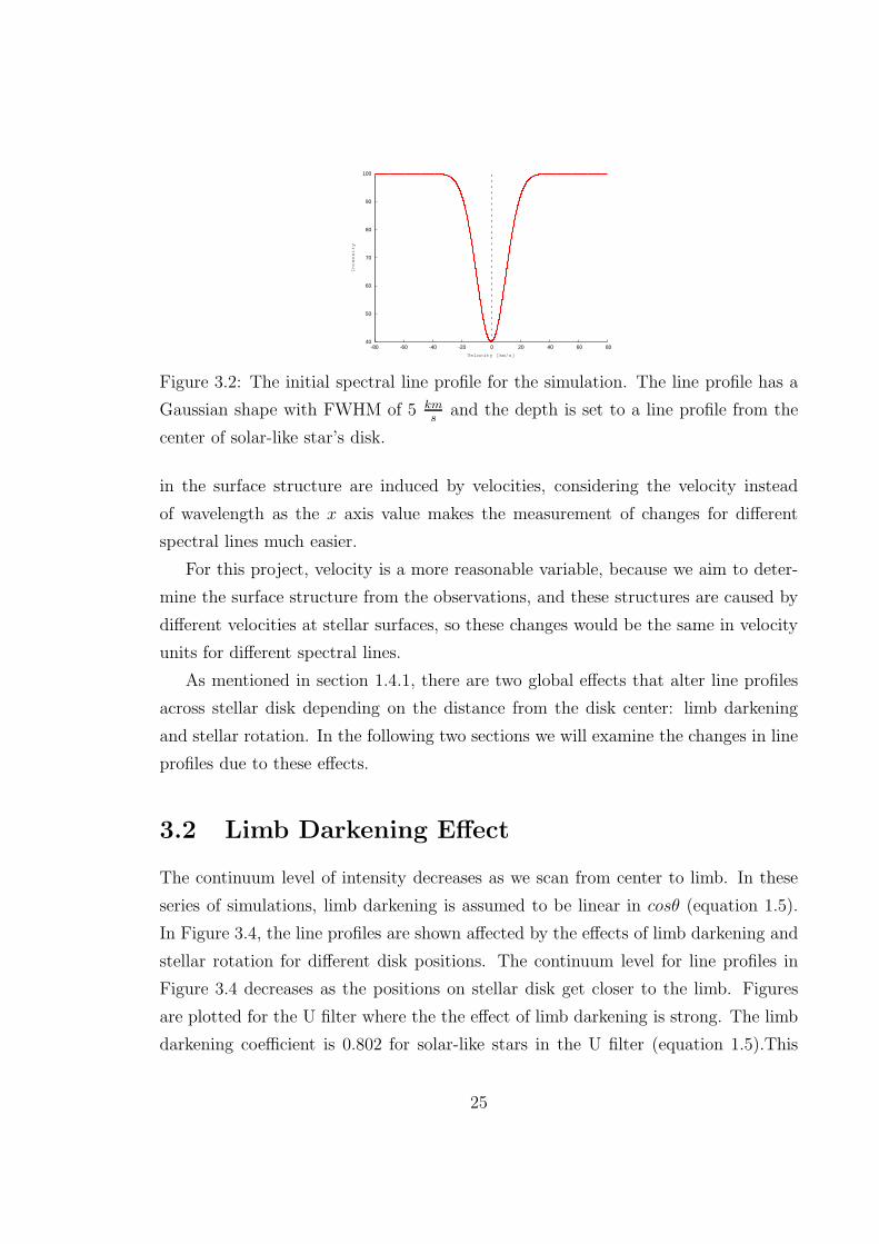
The second step is to assign a line profile to each pixel. The initial line profile

is plotted in Figure 3.2. This idealized line has a Gaussian shape, with depth of

40 percent and Full Width of Half Maximum (FWHM) of 5 km

s. A line profile with

these particulars is close to an average solar spectral line. The function which is used

to produce this line is:

I(v) = 1− A1√2πσ2

exp(−(x − x)2

2σ2) (3.1)

Where I is the intensity of the line, A is a coefficient to provide the right depth,

σ is the standard deviation and x is the mean value.

Since we measure variables on x axis relative to the center of the spectral line,

it is possible to use the velocity instead of wavelength on x axis. Since the changes

24

40

50

60

70

80

90

100

-80 -60 -40 -20 0 20 40 60 80Intensity

Velocity [km/s]

Figure 3.2: The initial spectral line profile for the simulation. The line profile has a

Gaussian shape with FWHM of 5 km

sand the depth is set to a line profile from the

center of solar-like star’s disk.

in the surface structure are induced by velocities, considering the velocity instead

of wavelength as the x axis value makes the measurement of changes for different

spectral lines much easier.

For this project, velocity is a more reasonable variable, because we aim to deter-

mine the surface structure from the observations, and these structures are caused by

different velocities at stellar surfaces, so these changes would be the same in velocity

units for different spectral lines.

As mentioned in section 1.4.1, there are two global effects that alter line profiles

across stellar disk depending on the distance from the disk center: limb darkening

and stellar rotation. In the following two sections we will examine the changes in line

profiles due to these effects.

3.2 Limb Darkening Effect

The continuum level of intensity decreases as we scan from center to limb. In these

series of simulations, limb darkening is assumed to be linear in cosθ (equation 1.5).

In Figure 3.4, the line profiles are shown affected by the effects of limb darkening and

stellar rotation for different disk positions. The continuum level for line profiles in

Figure 3.4 decreases as the positions on stellar disk get closer to the limb. Figures

are plotted for the U filter where the the effect of limb darkening is strong. The limb

darkening coefficient is 0.802 for solar-like stars in the U filter (equation 1.5).This

25

0

20

40

60

80

100

-100 -50 0 50 100Intensity

Velocity [km/s]

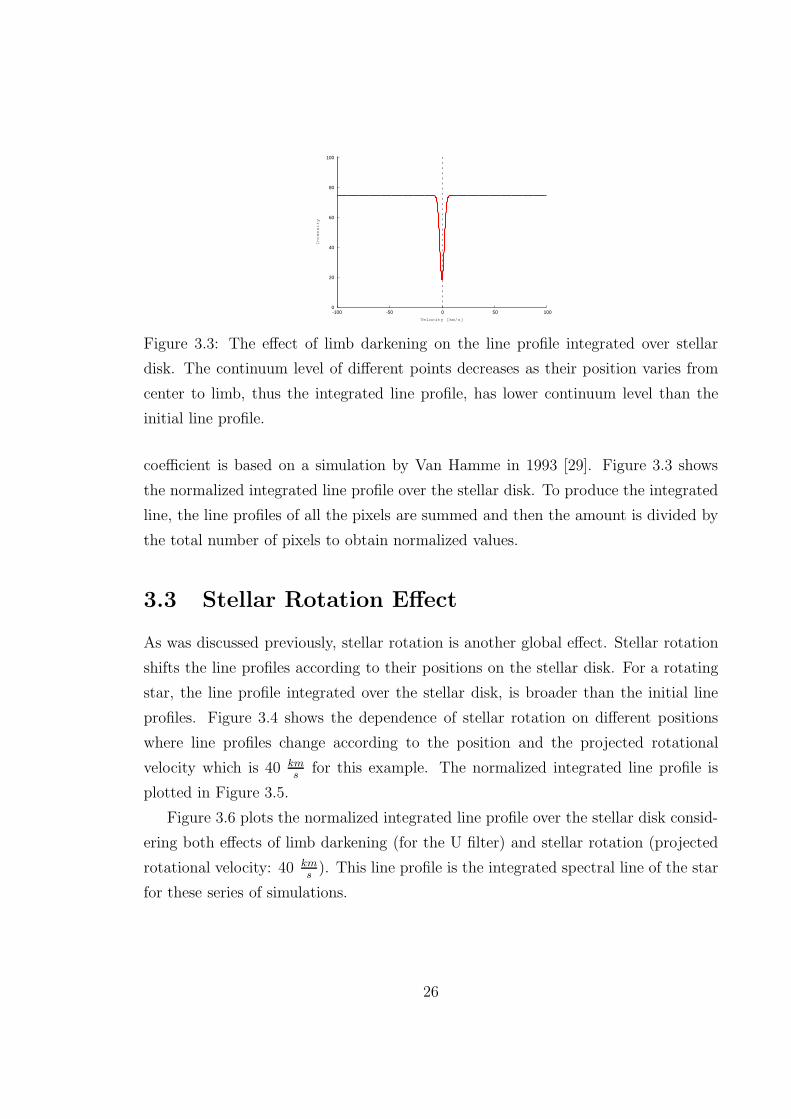
Figure 3.3: The effect of limb darkening on the line profile integrated over stellar

disk. The continuum level of different points decreases as their position varies from

center to limb, thus the integrated line profile, has lower continuum level than the

initial line profile.

coefficient is based on a simulation by Van Hamme in 1993 [29]. Figure 3.3 shows

the normalized integrated line profile over the stellar disk. To produce the integrated

line, the line profiles of all the pixels are summed and then the amount is divided by

the total number of pixels to obtain normalized values.

3.3 Stellar Rotation Effect

As was discussed previously, stellar rotation is another global effect. Stellar rotation

shifts the line profiles according to their positions on the stellar disk. For a rotating

star, the line profile integrated over the stellar disk, is broader than the initial line

profiles. Figure 3.4 shows the dependence of stellar rotation on different positions

where line profiles change according to the position and the projected rotational

velocity which is 40 kms

for this example. The normalized integrated line profile is

plotted in Figure 3.5.

Figure 3.6 plots the normalized integrated line profile over the stellar disk consid-

ering both effects of limb darkening (for the U filter) and stellar rotation (projected

rotational velocity: 40 kms). This line profile is the integrated spectral line of the star

for these series of simulations.

26

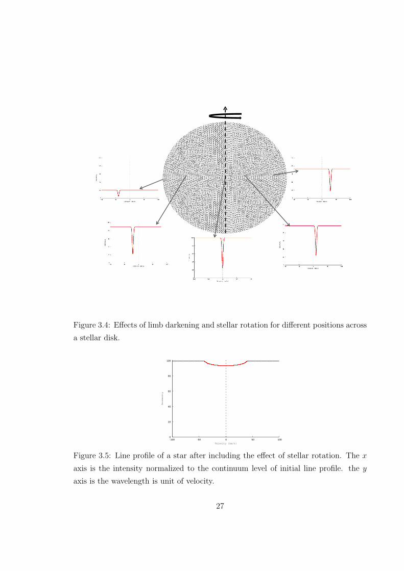
Figure 3.4: Effects of limb darkening and stellar rotation for different positions across

a stellar disk.

0

20

40

60

80

100

-100 -50 0 50 100

Intensity

Velocity [km/s]

Figure 3.5: Line profile of a star after including the effect of stellar rotation. The x

axis is the intensity normalized to the continuum level of initial line profile. the y

axis is the wavelength is unit of velocity.

27

0

20

40

60

80

100

-100 -50 0 50 100Intensity

Velocity [km/s]

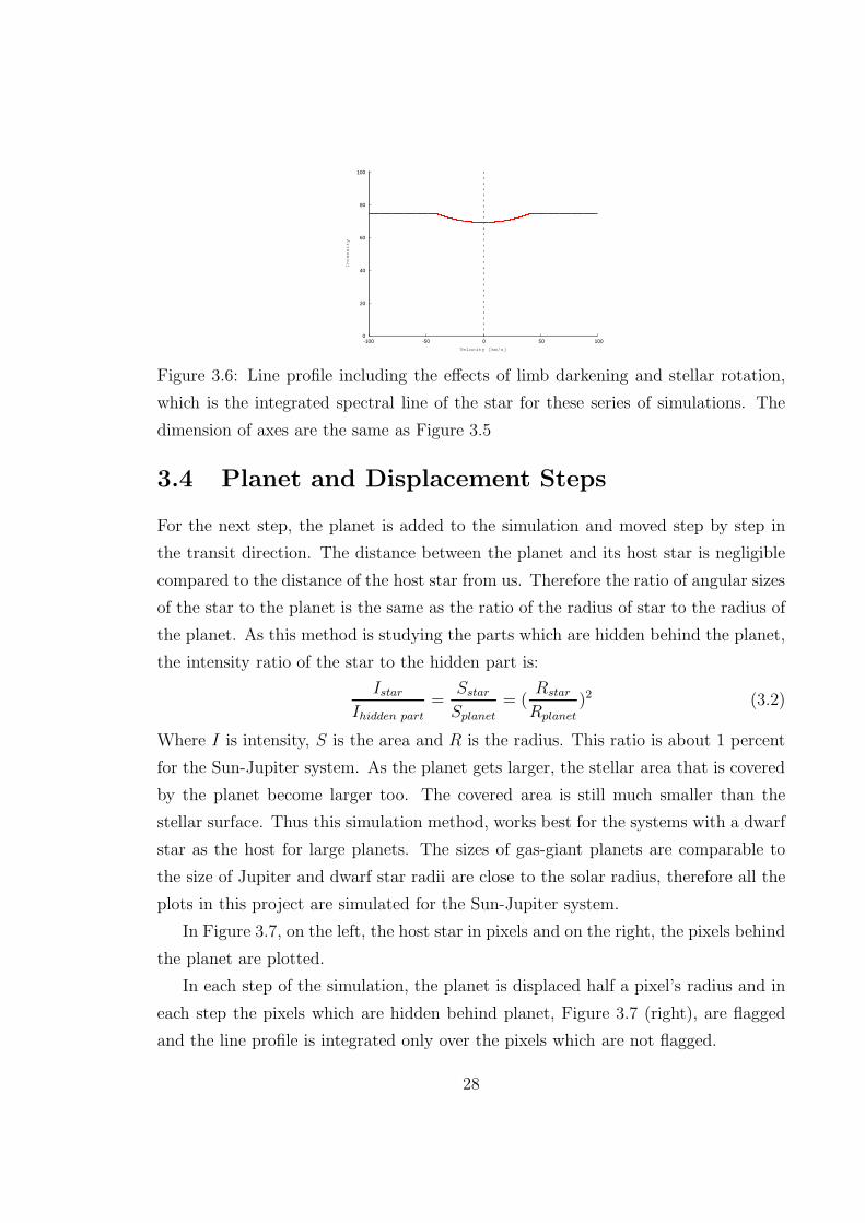
Figure 3.6: Line profile including the effects of limb darkening and stellar rotation,

which is the integrated spectral line of the star for these series of simulations. The

dimension of axes are the same as Figure 3.5

3.4 Planet and Displacement Steps

For the next step, the planet is added to the simulation and moved step by step in

the transit direction. The distance between the planet and its host star is negligible

compared to the distance of the host star from us. Therefore the ratio of angular sizes

of the star to the planet is the same as the ratio of the radius of star to the radius of

the planet. As this method is studying the parts which are hidden behind the planet,

the intensity ratio of the star to the hidden part is:

Istar

Ihidden part

=Sstar

Splanet

= (Rstar

Rplanet

)2 (3.2)

Where I is intensity, S is the area and R is the radius. This ratio is about 1 percent

for the Sun-Jupiter system. As the planet gets larger, the stellar area that is covered

by the planet become larger too. The covered area is still much smaller than the

stellar surface. Thus this simulation method, works best for the systems with a dwarf

star as the host for large planets. The sizes of gas-giant planets are comparable to

the size of Jupiter and dwarf star radii are close to the solar radius, therefore all the

plots in this project are simulated for the Sun-Jupiter system.

In Figure 3.7, on the left, the host star in pixels and on the right, the pixels behind

the planet are plotted.

In each step of the simulation, the planet is displaced half a pixel’s radius and in

each step the pixels which are hidden behind planet, Figure 3.7 (right), are flagged

and the line profile is integrated only over the pixels which are not flagged.

28

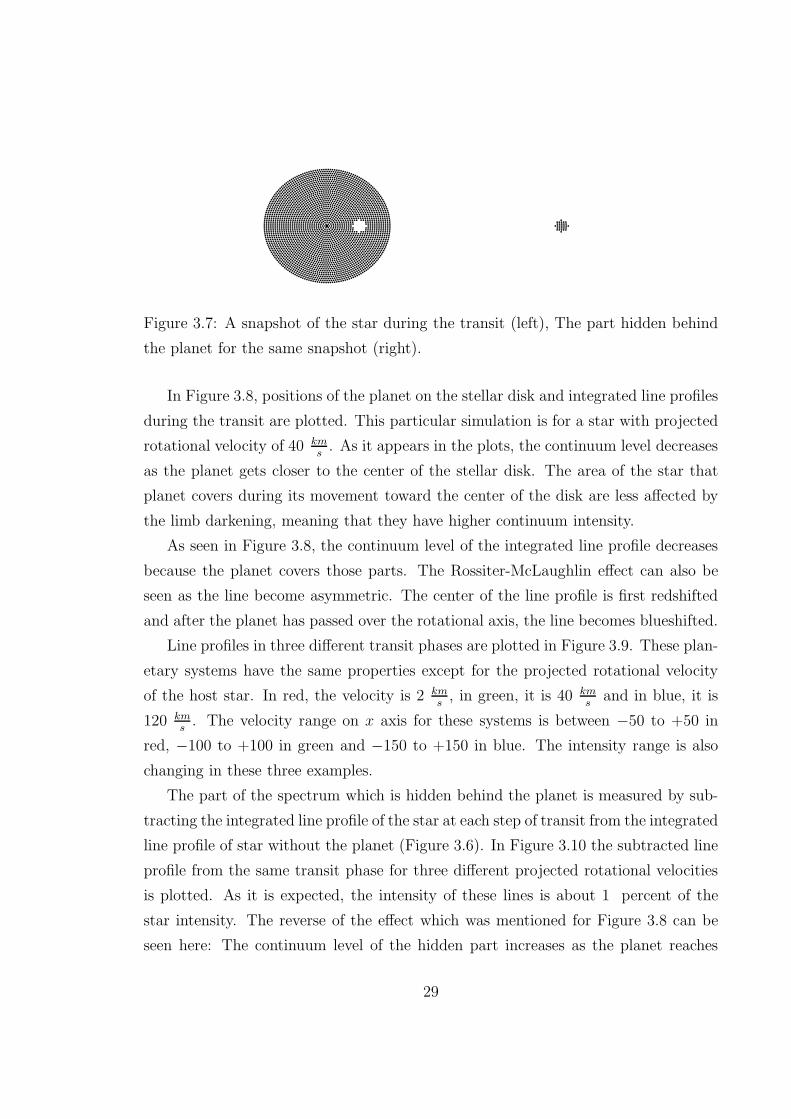
Figure 3.7: A snapshot of the star during the transit (left), The part hidden behind

the planet for the same snapshot (right).

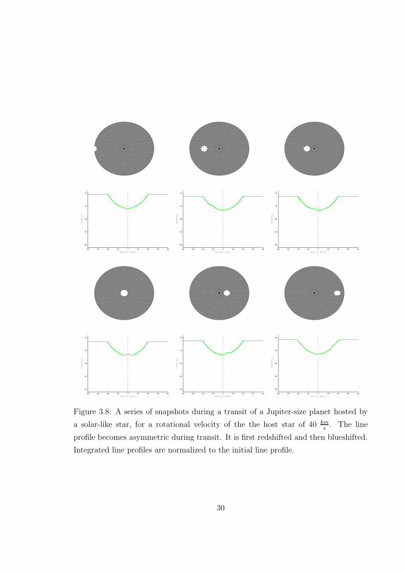
In Figure 3.8, positions of the planet on the stellar disk and integrated line profiles

during the transit are plotted. This particular simulation is for a star with projected

rotational velocity of 40 km

s. As it appears in the plots, the continuum level decreases

as the planet gets closer to the center of the stellar disk. The area of the star that

planet covers during its movement toward the center of the disk are less affected by

the limb darkening, meaning that they have higher continuum intensity.

As seen in Figure 3.8, the continuum level of the integrated line profile decreases

because the planet covers those parts. The Rossiter-McLaughlin effect can also be

seen as the line become asymmetric. The center of the line profile is first redshifted

and after the planet has passed over the rotational axis, the line becomes blueshifted.

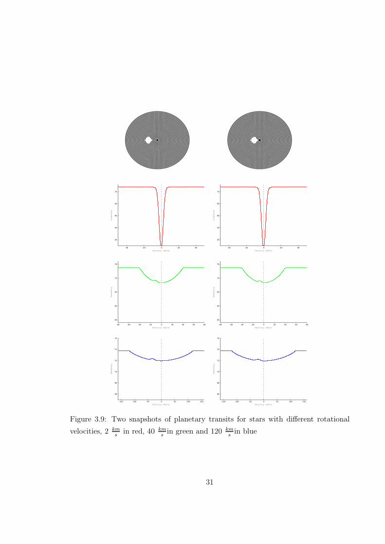
Line profiles in three different transit phases are plotted in Figure 3.9. These plan-

etary systems have the same properties except for the projected rotational velocity

of the host star. In red, the velocity is 2 km

s, in green, it is 40 km

sand in blue, it is

120 kms. The velocity range on x axis for these systems is between −50 to +50 in

red, −100 to +100 in green and −150 to +150 in blue. The intensity range is also

changing in these three examples.

The part of the spectrum which is hidden behind the planet is measured by sub-

tracting the integrated line profile of the star at each step of transit from the integrated

line profile of star without the planet (Figure 3.6). In Figure 3.10 the subtracted line

profile from the same transit phase for three different projected rotational velocities

is plotted. As it is expected, the intensity of these lines is about 1 percent of the

star intensity. The reverse of the effect which was mentioned for Figure 3.8 can be

seen here: The continuum level of the hidden part increases as the planet reaches

29

55

60

65

70

75

-80 -60 -40 -20 0 20 40 60 80

Intensity

Velocity [km/s]

55

60

65

70

75

-80 -60 -40 -20 0 20 40 60 80

Intensity

Velocity [km/s]

55

60

65

70

75

-80 -60 -40 -20 0 20 40 60 80

Intensity

Velocity [km/s]

55

60

65

70

75

-80 -60 -40 -20 0 20 40 60 80

Intensity

Velocity [km/s]

55

60

65

70

75

-80 -60 -40 -20 0 20 40 60 80

Intensity

Velocity [km/s]

55

60

65

70

75

-80 -60 -40 -20 0 20 40 60 80

Intensity

Velocity [km/s]

Figure 3.8: A series of snapshots during a transit of a Jupiter-size planet hosted by

a solar-like star, for a rotational velocity of the the host star of 40 km

s. The line

profile becomes asymmetric during transit. It is first redshifted and then blueshifted.

Integrated line profiles are normalized to the initial line profile.

30

30

40

50

60

70

-40 -20 0 20 40

Intensity

Velocity [km/s]

30

40

50

60

70

-40 -20 0 20 40

Intensity

Velocity [km/s]

55

60

65

70

75

-80 -60 -40 -20 0 20 40 60 80

Intensity

Velocity [km/s]

55

60

65

70

75

-80 -60 -40 -20 0 20 40 60 80

Intensity

Velocity [km/s]

66

68

70

72

74

76

-150 -100 -50 0 50 100 150

Intensity

Velocity [km/s]

66

68

70

72

74

76

-150 -100 -50 0 50 100 150

Intensity

Velocity [km/s]

Figure 3.9: Two snapshots of planetary transits for stars with different rotational

velocities, 2 km

sin red, 40 km

sin green and 120 km

sin blue

31

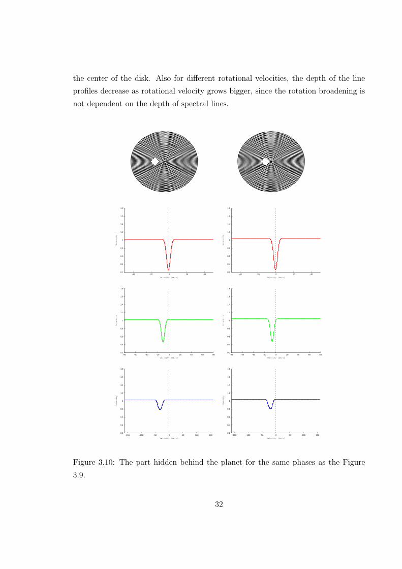
the center of the disk. Also for different rotational velocities, the depth of the line

profiles decrease as rotational velocity grows bigger, since the rotation broadening is

not dependent on the depth of spectral lines.

0.2

0.4

0.6

0.8

1

1.2

1.4

1.6

1.8

-40 -20 0 20 40

Intensity

Velocity [km/s]

0.2

0.4

0.6

0.8

1

1.2

1.4

1.6

1.8

-40 -20 0 20 40

Intensity

Velocity [km/s]

0.2

0.4

0.6

0.8

1

1.2

1.4

1.6

1.8

-80 -60 -40 -20 0 20 40 60 80

Intensity

Velocity [km/s]

0.2

0.4

0.6

0.8

1

1.2

1.4

1.6

1.8

-80 -60 -40 -20 0 20 40 60 80

Intensity

Velocity [km/s]

0.2

0.4

0.6

0.8

1

1.2

1.4

1.6

1.8

-150 -100 -50 0 50 100 150

Intensity

Velocity [km/s]

0.2

0.4

0.6

0.8

1

1.2

1.4

1.6

1.8

-150 -100 -50 0 50 100 150

Intensity

Velocity [km/s]

Figure 3.10: The part hidden behind the planet for the same phases as the Figure

3.9.

32

3.5 Instrumental Effects and Finite Resolution

In observations, there are effects caused by telescopes and attached instruments which

limits the quality of observations, such as bias levels in CCDs, inhomogeneous sensi-

tivity of the CCD pixels, etc. Although it is possible to remove some of these harmful

effects, there are some effects which we are unable to erase. The most important ones

in spectroscopy are finite spectral resolution of the spectrograph and photon noise of

the signal. An approximation of these effects has been added to the simulations.

3.5.1 Spectral Resolution

To approximate the finite spectral resolution ( λ∆λ

), the data points were convolved

with a series of Gaussian distributions with full width of half maximum equals to

the assumed spectrograph resolution. The limit for calculating the wings of the

Gaussian distribution is where the intensity at the wing reaches 0.01 percent of an

ideal continuum level. This is a reasonable value since the line hidden behind the

planet has the intensity about 1 percent of the continuum level (Figure 3.10).

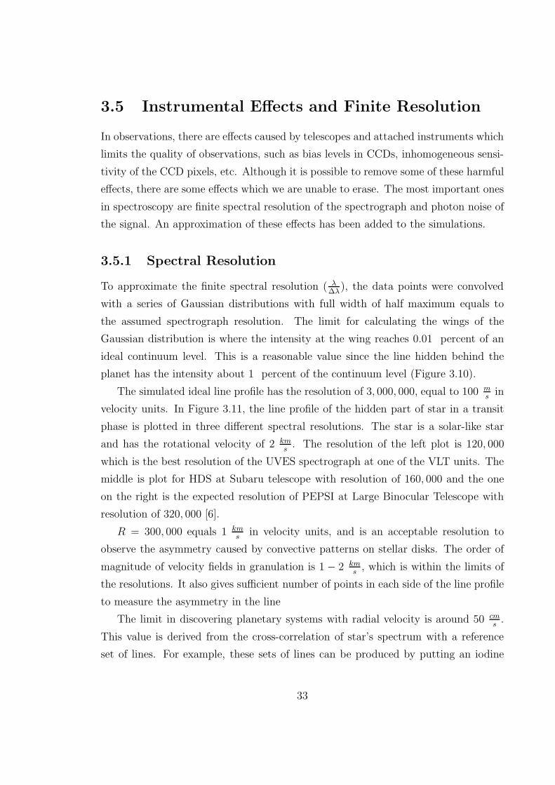
The simulated ideal line profile has the resolution of 3, 000, 000, equal to 100 msin

velocity units. In Figure 3.11, the line profile of the hidden part of star in a transit

phase is plotted in three different spectral resolutions. The star is a solar-like star

and has the rotational velocity of 2 km

s. The resolution of the left plot is 120, 000

which is the best resolution of the UVES spectrograph at one of the VLT units. The

middle is plot for HDS at Subaru telescope with resolution of 160, 000 and the one

on the right is the expected resolution of PEPSI at Large Binocular Telescope with

resolution of 320, 000 [6].

R = 300, 000 equals 1 kms

in velocity units, and is an acceptable resolution to

observe the asymmetry caused by convective patterns on stellar disks. The order of

magnitude of velocity fields in granulation is 1 − 2 kms, which is within the limits of

the resolutions. It also gives sufficient number of points in each side of the line profile

to measure the asymmetry in the line

The limit in discovering planetary systems with radial velocity is around 50 cm

s.

This value is derived from the cross-correlation of star’s spectrum with a reference

set of lines. For example, these sets of lines can be produced by putting an iodine

33

0.2

0.4

0.6

0.8

1

1.2

1.4

1.6

-40 -20 0 20 40

Intensity

Velocity [km/s]

0.2

0.4

0.6

0.8

1

1.2

1.4

1.6

-40 -20 0 20 40

Intensity

Velocity [km/s]

0.2

0.4

0.6

0.8

1

1.2

1.4

1.6

-40 -20 0 20 40

Intensity

Velocity [km/s]

Figure 3.11: The line profile of the hidden part of a star with rotational velocity of

2 km

sin three spectral resolutions. spectral resolution is 120, 000 at top left , 160, 000

at top right and 320, 000 in the bottom image.

34

cell in front of the spectrograph. The stellar light passes through this cell before

reaching the spectrograph and a series of spectral lines is superposed onto the stellar

spectrum. However, since we are looking at the full line profiles, we cannot easily use

the cross-correlation method and our measurements are limited by the spectrograph

resolution.

3.5.2 Noise

According to the central limit theorem, the sum of a large number of variables will

have approximately a normal Gaussian distribution. Therefore for estimating the

photon noise, normal-distributed noise has been added to the signal of the star

with/without a planet before subtraction. To show how the noise affects the line

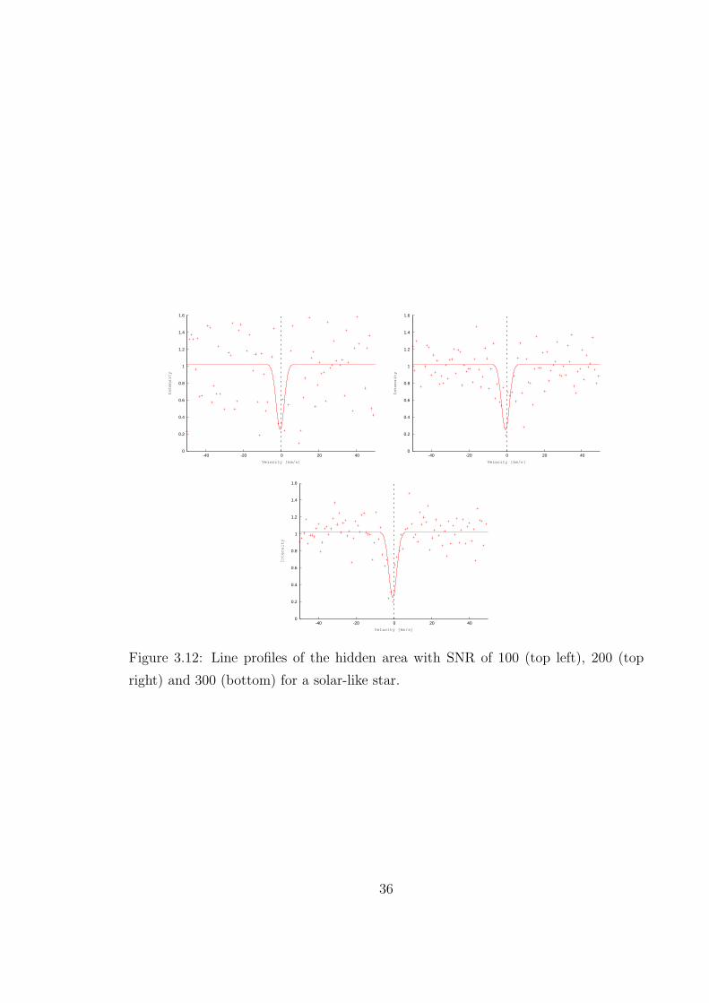
profile, Figure 3.12 is plotted. The solid line is the line profile of the hidden area of

the star without considering the effect of spectral resolution or noise and the points

are the data after convolving the line with resolution of 320, 000 and considering the

effect of noise with an assumed Signal-to-Noise-Ratio (SNR). The noise is added be-

fore subtraction thus SNR is related to the signal of the integrated line over the stellar

disk. On the left plot the SNR is 100 where the line profile cannot be detected. In

the middle, the SNR is 200, the line profile is detectable but still is too noisy for our

needs. On the right the SNR is 300 which is the estimation of the highest SNR that

we can obtain with resolution of 300, 000 during an observation with short exposure

times. Planetary transit times are of the order of hours, so to obtain the spectrum of

different parts, the exposure times must be short.

35

0

0.2

0.4

0.6

0.8

1

1.2

1.4

1.6

-40 -20 0 20 40

Intensity

Velocity [km/s]

0

0.2

0.4

0.6

0.8

1

1.2

1.4

1.6

-40 -20 0 20 40

Intensity

Velocity [km/s]

0

0.2

0.4

0.6

0.8

1

1.2

1.4

1.6

-40 -20 0 20 40

Intensity

Velocity [km/s]

Figure 3.12: Line profiles of the hidden area with SNR of 100 (top left), 200 (top

right) and 300 (bottom) for a solar-like star.

36

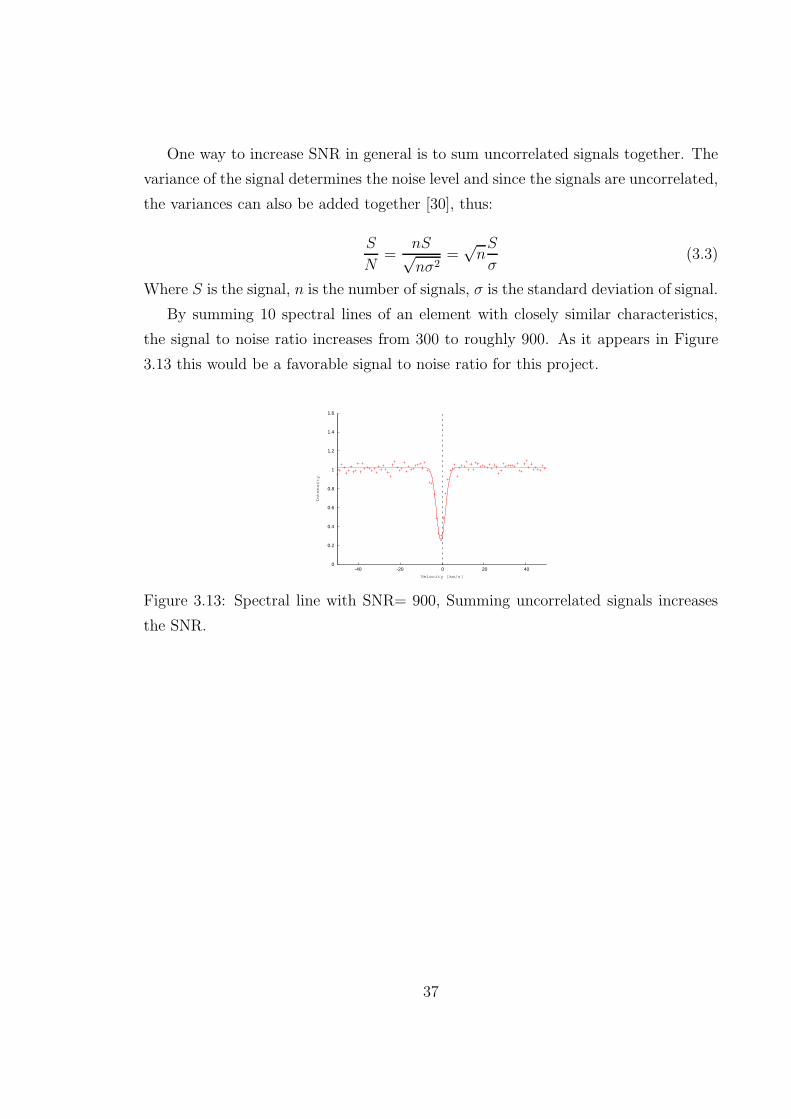
One way to increase SNR in general is to sum uncorrelated signals together. The

variance of the signal determines the noise level and since the signals are uncorrelated,

the variances can also be added together [30], thus:

S

N=

nS√nσ2

=√nS

σ(3.3)

Where S is the signal, n is the number of signals, σ is the standard deviation of signal.

By summing 10 spectral lines of an element with closely similar characteristics,

the signal to noise ratio increases from 300 to roughly 900. As it appears in Figure

3.13 this would be a favorable signal to noise ratio for this project.

0

0.2

0.4

0.6

0.8

1

1.2

1.4

1.6

-40 -20 0 20 40

Intensity

Velocity [km/s]

Figure 3.13: Spectral line with SNR= 900, Summing uncorrelated signals increases

the SNR.

37

In the series of plots in Figure 3.14, the line profiles have spectral resolution of

320, 000 and thr SNR of 300 for a spectral line.

0.2

0.4

0.6

0.8

1

1.2

1.4

1.6

1.8

-40 -20 0 20 40

Intensity

Velocity [km/s]

0.2

0.4

0.6

0.8

1

1.2

1.4

1.6

1.8

-40 -20 0 20 40

Intensity

Velocity [km/s]

0.2

0.4

0.6

0.8

1

1.2

1.4

1.6

1.8

-80 -60 -40 -20 0 20 40 60 80

Intensity

Velocity [km/s]

0.2

0.4

0.6

0.8

1

1.2

1.4

1.6

1.8

-80 -60 -40 -20 0 20 40 60 80

Intensity

Velocity [km/s]

0.2

0.4

0.6

0.8

1

1.2

1.4

1.6

1.8

-150 -100 -50 0 50 100 150

Intensity

Velocity [km/s]

0.2

0.4

0.6

0.8

1

1.2

1.4

1.6

1.8

-150 -100 -50 0 50 100 150

Intensity

Velocity [km/s]

Figure 3.14: Line profiles for two different transit phases, with the spectral resolution

of 320, 000 and SNR of 300. Different colors represent different stellar rotational

velocities.

38

Chapter 4

Simulation–Realistic Line Profile

4.1 Initial Conditions

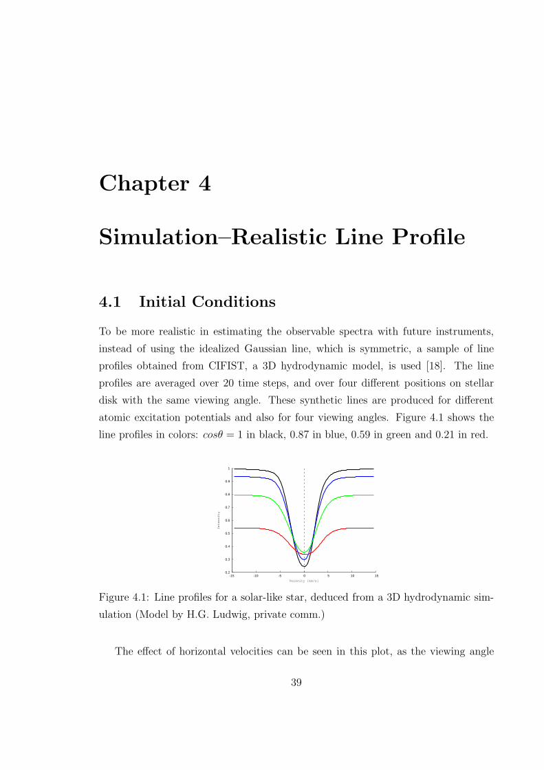
To be more realistic in estimating the observable spectra with future instruments,

instead of using the idealized Gaussian line, which is symmetric, a sample of line

profiles obtained from CIFIST, a 3D hydrodynamic model, is used [18]. The line

profiles are averaged over 20 time steps, and over four different positions on stellar

disk with the same viewing angle. These synthetic lines are produced for different

atomic excitation potentials and also for four viewing angles. Figure 4.1 shows the

line profiles in colors: cosθ = 1 in black, 0.87 in blue, 0.59 in green and 0.21 in red.

0.2

0.3

0.4

0.5

0.6

0.7

0.8

0.9

1

-15 -10 -5 0 5 10 15

Intensity

Velocity [km/s]

Figure 4.1: Line profiles for a solar-like star, deduced from a 3D hydrodynamic sim-

ulation (Model by H.G. Ludwig, private comm.)

The effect of horizontal velocities can be seen in this plot, as the viewing angle

39

become larger, or as we look closer to the limb, the line profiles become broadened

and shallower. Also the continuum level of these lines decreases which is the effect

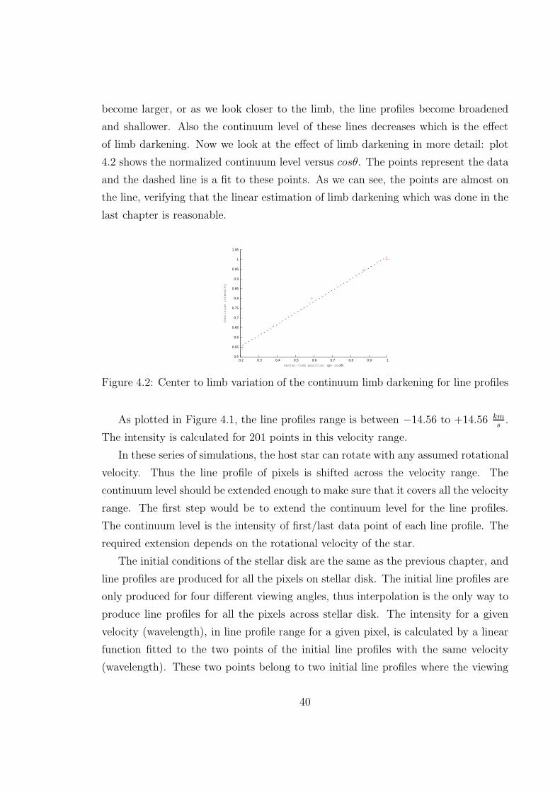
of limb darkening. Now we look at the effect of limb darkening in more detail: plot

4.2 shows the normalized continuum level versus cosθ. The points represent the data

and the dashed line is a fit to these points. As we can see, the points are almost on

the line, verifying that the linear estimation of limb darkening which was done in the

last chapter is reasonable.

0.5

0.55

0.6

0.65

0.7

0.75

0.8

0.85

0.9

0.95

1

1.05

0.2 0.3 0.4 0.5 0.6 0.7 0.8 0.9 1

Continuum intensity

Center-limb position (µ= cosθ)

Figure 4.2: Center to limb variation of the continuum limb darkening for line profiles

As plotted in Figure 4.1, the line profiles range is between −14.56 to +14.56 km

s.

The intensity is calculated for 201 points in this velocity range.

In these series of simulations, the host star can rotate with any assumed rotational

velocity. Thus the line profile of pixels is shifted across the velocity range. The

continuum level should be extended enough to make sure that it covers all the velocity

range. The first step would be to extend the continuum level for the line profiles.

The continuum level is the intensity of first/last data point of each line profile. The

required extension depends on the rotational velocity of the star.

The initial conditions of the stellar disk are the same as the previous chapter, and

line profiles are produced for all the pixels on stellar disk. The initial line profiles are

only produced for four different viewing angles, thus interpolation is the only way to

produce line profiles for all the pixels across stellar disk. The intensity for a given

velocity (wavelength), in line profile range for a given pixel, is calculated by a linear

function fitted to the two points of the initial line profiles with the same velocity

(wavelength). These two points belong to two initial line profiles where the viewing

40

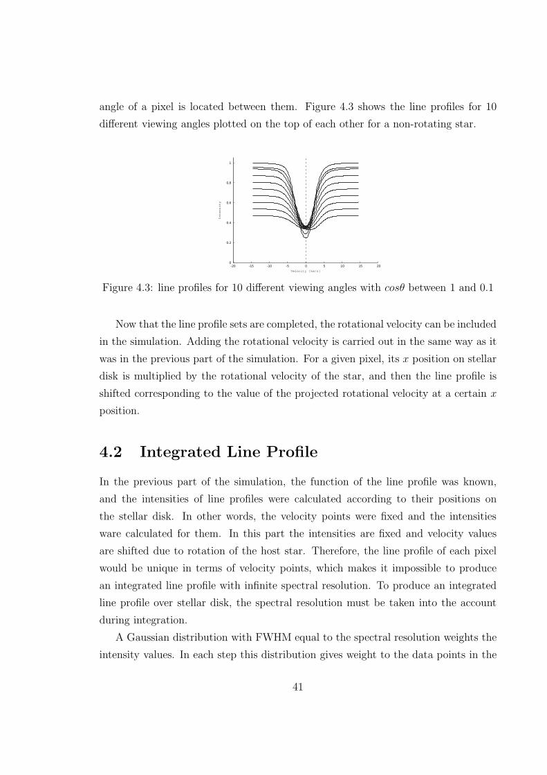
angle of a pixel is located between them. Figure 4.3 shows the line profiles for 10

different viewing angles plotted on the top of each other for a non-rotating star.

0

0.2

0.4

0.6

0.8

1

-20 -15 -10 -5 0 5 10 15 20

Intensity

Velocity [km/s]

Figure 4.3: line profiles for 10 different viewing angles with cosθ between 1 and 0.1

Now that the line profile sets are completed, the rotational velocity can be included

in the simulation. Adding the rotational velocity is carried out in the same way as it

was in the previous part of the simulation. For a given pixel, its x position on stellar

disk is multiplied by the rotational velocity of the star, and then the line profile is

shifted corresponding to the value of the projected rotational velocity at a certain x

position.

4.2 Integrated Line Profile

In the previous part of the simulation, the function of the line profile was known,

and the intensities of line profiles were calculated according to their positions on

the stellar disk. In other words, the velocity points were fixed and the intensities

ware calculated for them. In this part the intensities are fixed and velocity values

are shifted due to rotation of the host star. Therefore, the line profile of each pixel

would be unique in terms of velocity points, which makes it impossible to produce

an integrated line profile with infinite spectral resolution. To produce an integrated

line profile over stellar disk, the spectral resolution must be taken into the account

during integration.

A Gaussian distribution with FWHM equal to the spectral resolution weights the

intensity values. In each step this distribution gives weight to the data points in the

41

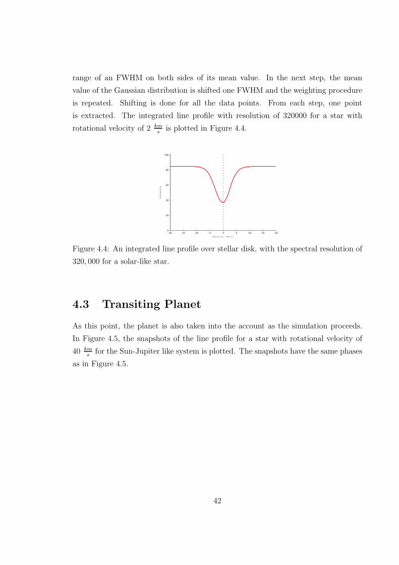
range of an FWHM on both sides of its mean value. In the next step, the mean

value of the Gaussian distribution is shifted one FWHM and the weighting procedure

is repeated. Shifting is done for all the data points. From each step, one point

is extracted. The integrated line profile with resolution of 320000 for a star with

rotational velocity of 2 km

sis plotted in Figure 4.4.

0

20

40

60

80

100

-20 -15 -10 -5 0 5 10 15 20

Intensity

Velocity [km/s]

Figure 4.4: An integrated line profile over stellar disk, with the spectral resolution of

320, 000 for a solar-like star.

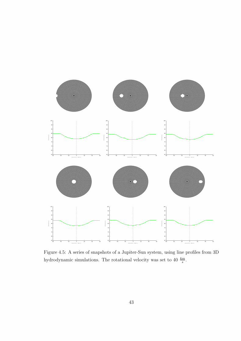
4.3 Transiting Planet

As this point, the planet is also taken into the account as the simulation proceeds.

In Figure 4.5, the snapshots of the line profile for a star with rotational velocity of

40 kms

for the Sun-Jupiter like system is plotted. The snapshots have the same phases

as in Figure 4.5.

42

60

65

70

75

80

85

90

95

100

-60 -40 -20 0 20 40 60

Intensity

Velocity [km/s]

60

65

70

75

80

85

90

95

100

-60 -40 -20 0 20 40 60

Intensity

Velocity [km/s]

60

65

70

75

80

85

90

95

100

-60 -40 -20 0 20 40 60

Intensity

Velocity [km/s]

60

65

70

75

80

85

90

95

100

-60 -40 -20 0 20 40 60

Intensity

Velocity [km/s]

60

65

70

75

80

85

90

95

100

-60 -40 -20 0 20 40 60

Intensity

Velocity [km/s]

60

65

70

75

80

85

90

95

100

-60 -40 -20 0 20 40 60

Intensity

Velocity [km/s]

Figure 4.5: A series of snapshots of a Jupiter-Sun system, using line profiles from 3D

hydrodynamic simulations. The rotational velocity was set to 40 km

s.

43

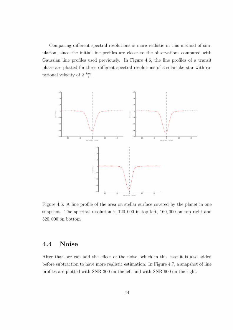
Comparing different spectral resolutions is more realistic in this method of sim-

ulation, since the initial line profiles are closer to the observations compared with

Gaussian line profiles used previously. In Figure 4.6, the line profiles of a transit

phase are plotted for three different spectral resolutions of a solar-like star with ro-

tational velocity of 2 km

s.

0.2

0.4

0.6

0.8

1

1.2

1.4

1.6

-20 -10 0 10 20

Intensity

Velocity [km/s]

0.2

0.4

0.6

0.8

1

1.2

1.4

1.6

-20 -10 0 10 20

Intensity

Velocity [km/s]

0.2

0.4

0.6

0.8

1

1.2

1.4

1.6

-20 -10 0 10 20

Intensity

Velocity [km/s]

Figure 4.6: A line profile of the area on stellar surface covered by the planet in one

snapshot. The spectral resolution is 120, 000 in top left, 160, 000 on top right and

320, 000 on bottom

4.4 Noise

After that, we can add the effect of the noise, which in this case it is also added

before subtraction to have more realistic estimation. In Figure 4.7, a snapshot of line

profiles are plotted with SNR 300 on the left and with SNR 900 on the right.

44

0

0.2

0.4

0.6

0.8

1

1.2

1.4

1.6

-20 -10 0 10 20

Intensity

Velocity [km/s]

0

0.2

0.4

0.6

0.8

1

1.2

1.4

1.6

-20 -10 0 10 20

Intensity

Velocity [km/s]

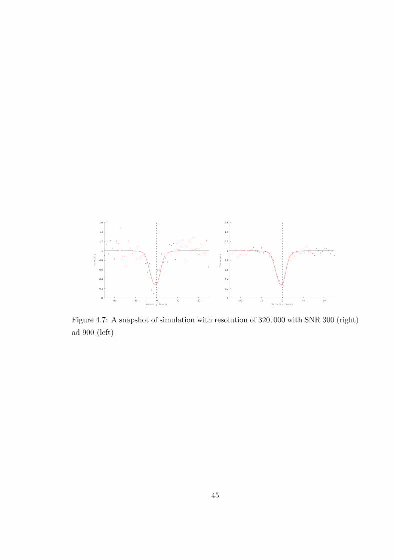
Figure 4.7: A snapshot of simulation with resolution of 320, 000 with SNR 300 (right)

ad 900 (left)

45

Chapter 5

Direct Imaging with E-ELT

In this chapter we are looking at possible diffraction-patterns limited imaging with

extremely large telescopes, and how intensity of an extended object would be affected.

5.1 Theory

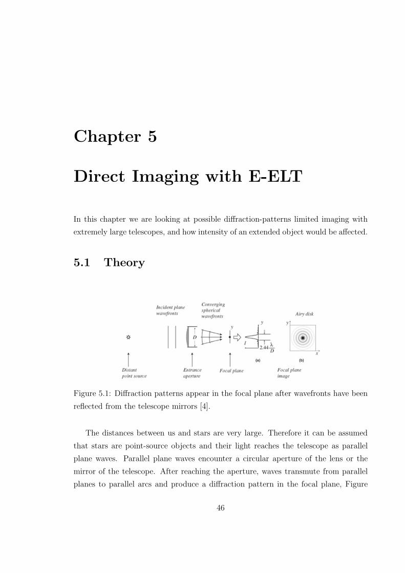
Figure 5.1: Diffraction patterns appear in the focal plane after wavefronts have been

reflected from the telescope mirrors [4].

The distances between us and stars are very large. Therefore it can be assumed

that stars are point-source objects and their light reaches the telescope as parallel

plane waves. Parallel plane waves encounter a circular aperture of the lens or the

mirror of the telescope. After reaching the aperture, waves transmute from parallel

planes to parallel arcs and produce a diffraction pattern in the focal plane, Figure

46

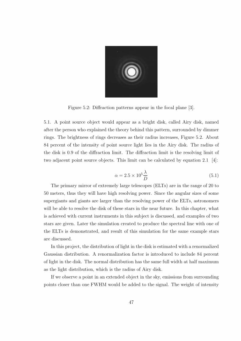
Figure 5.2: Diffraction patterns appear in the focal plane [3].

5.1. A point source object would appear as a bright disk, called Airy disk, named

after the person who explained the theory behind this pattern, surrounded by dimmer

rings. The brightness of rings decreases as their radius increases, Figure 5.2. About

84 percent of the intensity of point source light lies in the Airy disk. The radius of

the disk is 0.9 of the diffraction limit. The diffraction limit is the resolving limit of

two adjacent point source objects. This limit can be calculated by equation 2.1 [4]:

α = 2.5× 105λ

D(5.1)

The primary mirror of extremely large telescopes (ELTs) are in the range of 20 to

50 meters, thus they will have high resolving power. Since the angular sizes of some

supergiants and giants are larger than the resolving power of the ELTs, astronomers

will be able to resolve the disk of these stars in the near future. In this chapter, what

is achieved with current instruments in this subject is discussed, and examples of two

stars are given. Later the simulation created to produce the spectral line with one of

the ELTs is demonstrated, and result of this simulation for the same example stars

are discussed.

In this project, the distribution of light in the disk is estimated with a renormalized

Gaussian distribution. A renormalization factor is introduced to include 84 percent

of light in the disk. The normal distribution has the same full width at half maximum

as the light distribution, which is the radius of Airy disk.

If we observe a point in an extended object in the sky, emissions from surrounding

points closer than one FWHM would be added to the signal. The weight of intensity

47

for each point can be calculated as a function of the distance from the observing

point. Since the sum of the intensity of the observing point across the Airy disk is

84 percent of its initial intensity, the weight for the intensity of observing point is 84

percent. For other points in the extended object, the weight distribution would have

the same shape as light distribution and the re-normalization factor is the ratio 84

percent to the maximum value of a normal distribution.

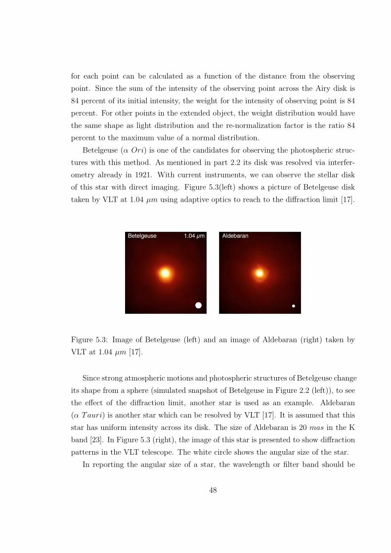
Betelgeuse (α Ori) is one of the candidates for observing the photospheric struc-

tures with this method. As mentioned in part 2.2 its disk was resolved via interfer-

ometry already in 1921. With current instruments, we can observe the stellar disk

of this star with direct imaging. Figure 5.3(left) shows a picture of Betelgeuse disk

taken by VLT at 1.04 µm using adaptive optics to reach to the diffraction limit [17].

Figure 5.3: Image of Betelgeuse (left) and an image of Aldebaran (right) taken by

VLT at 1.04 µm [17].

Since strong atmospheric motions and photospheric structures of Betelgeuse change

its shape from a sphere (simulated snapshot of Betelgeuse in Figure 2.2 (left)), to see

the effect of the diffraction limit, another star is used as an example. Aldebaran

(α Tauri) is another star which can be resolved by VLT [17]. It is assumed that this

star has uniform intensity across its disk. The size of Aldebaran is 20 mas in the K

band [23]. In Figure 5.3 (right), the image of this star is presented to show diffraction

patterns in the VLT telescope. The white circle shows the angular size of the star.

In reporting the angular size of a star, the wavelength or filter band should be

48

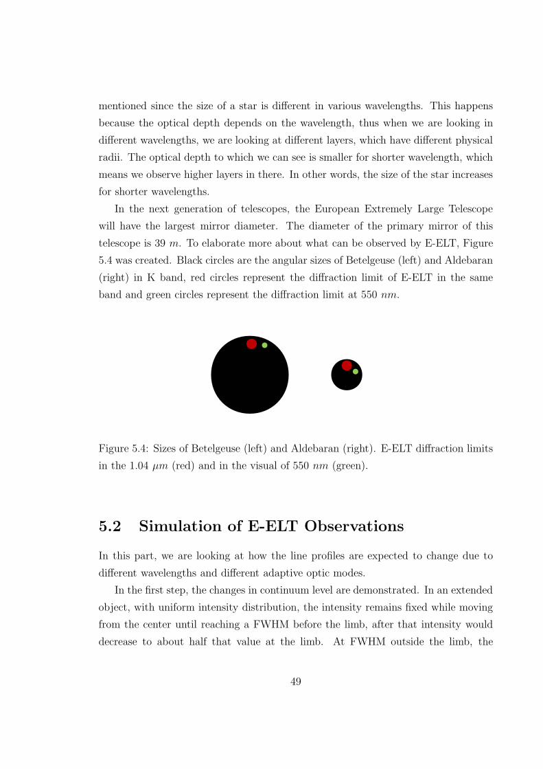
mentioned since the size of a star is different in various wavelengths. This happens

because the optical depth depends on the wavelength, thus when we are looking in

different wavelengths, we are looking at different layers, which have different physical

radii. The optical depth to which we can see is smaller for shorter wavelength, which

means we observe higher layers in there. In other words, the size of the star increases

for shorter wavelengths.

In the next generation of telescopes, the European Extremely Large Telescope

will have the largest mirror diameter. The diameter of the primary mirror of this

telescope is 39 m. To elaborate more about what can be observed by E-ELT, Figure

5.4 was created. Black circles are the angular sizes of Betelgeuse (left) and Aldebaran

(right) in K band, red circles represent the diffraction limit of E-ELT in the same

band and green circles represent the diffraction limit at 550 nm.

Figure 5.4: Sizes of Betelgeuse (left) and Aldebaran (right). E-ELT diffraction limits

in the 1.04 µm (red) and in the visual of 550 nm (green).

5.2 Simulation of E-ELT Observations

In this part, we are looking at how the line profiles are expected to change due to

different wavelengths and different adaptive optic modes.

In the first step, the changes in continuum level are demonstrated. In an extended

object, with uniform intensity distribution, the intensity remains fixed while moving

from the center until reaching a FWHM before the limb, after that intensity would

decrease to about half that value at the limb. At FWHM outside the limb, the

49

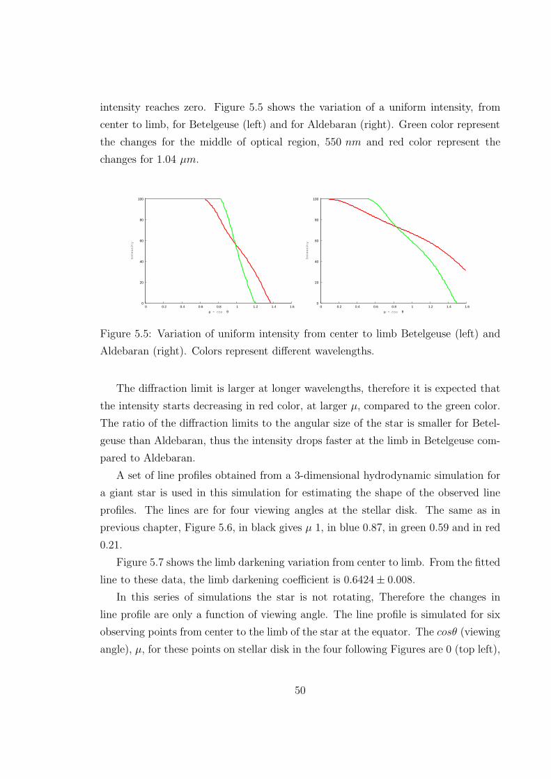
intensity reaches zero. Figure 5.5 shows the variation of a uniform intensity, from

center to limb, for Betelgeuse (left) and for Aldebaran (right). Green color represent

the changes for the middle of optical region, 550 nm and red color represent the

changes for 1.04 µm.

0

20

40

60

80

100

0 0.2 0.4 0.6 0.8 1 1.2 1.4 1.6

Intensity

µ = cos θ

0

20

40

60

80

100

0 0.2 0.4 0.6 0.8 1 1.2 1.4 1.6Intensity

µ = cos θ

Figure 5.5: Variation of uniform intensity from center to limb Betelgeuse (left) and

Aldebaran (right). Colors represent different wavelengths.

The diffraction limit is larger at longer wavelengths, therefore it is expected that

the intensity starts decreasing in red color, at larger µ, compared to the green color.

The ratio of the diffraction limits to the angular size of the star is smaller for Betel-

geuse than Aldebaran, thus the intensity drops faster at the limb in Betelgeuse com-

pared to Aldebaran.

A set of line profiles obtained from a 3-dimensional hydrodynamic simulation for

a giant star is used in this simulation for estimating the shape of the observed line

profiles. The lines are for four viewing angles at the stellar disk. The same as in

previous chapter, Figure 5.6, in black gives µ 1, in blue 0.87, in green 0.59 and in red

0.21.

Figure 5.7 shows the limb darkening variation from center to limb. From the fitted

line to these data, the limb darkening coefficient is 0.6424± 0.008.

In this series of simulations the star is not rotating, Therefore the changes in

line profile are only a function of viewing angle. The line profile is simulated for six

observing points from center to the limb of the star at the equator. The cosθ (viewing

angle), µ, for these points on stellar disk in the four following Figures are 0 (top left),

50

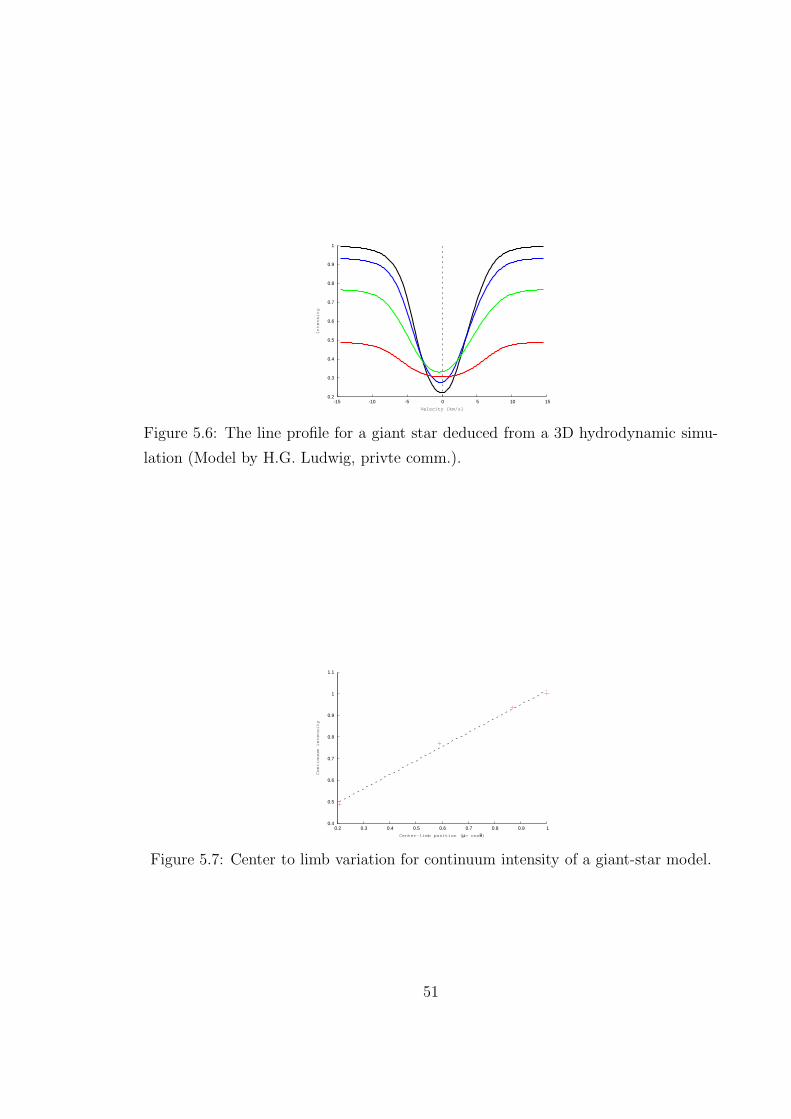
0.2

0.3

0.4

0.5

0.6

0.7

0.8

0.9

1

-15 -10 -5 0 5 10 15

Intensity

Velocity [km/s]

Figure 5.6: The line profile for a giant star deduced from a 3D hydrodynamic simu-

lation (Model by H.G. Ludwig, privte comm.).

0.4

0.5

0.6

0.7

0.8

0.9

1

1.1

0.2 0.3 0.4 0.5 0.6 0.7 0.8 0.9 1

Continuum intensity

Center-limb position (µ= cosθ)

Figure 5.7: Center to limb variation for continuum intensity of a giant-star model.

51

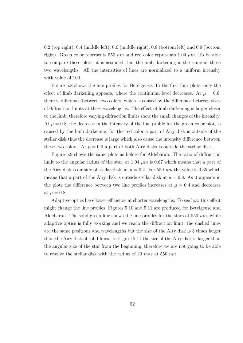
0.2 (top right), 0.4 (middle left), 0.6 (middle right), 0.8 (bottom left) and 0.9 (bottom

right). Green color represents 550 nm and red color represents 1.04 µm. To be able

to compare these plots, it is assumed that the limb darkening is the same at these

two wavelengths. All the intensities of lines are normalized to a uniform intensity

with value of 100.

Figure 5.8 shows the line profiles for Betelgeuse. In the first four plots, only the

effect of limb darkening appears, where the continuum level decreases. At µ = 0.6,

there is difference between two colors, which is caused by the difference between sizes

of diffraction limits at these wavelengths. The effect of limb darkening is larger closer

to the limb, therefore varying diffraction limits show the small changes of the intensity.

At µ = 0.8, the decrease in the intensity of the line profile for the green color plot, is

caused by the limb darkening; for the red color a part of Airy disk is outside of the

stellar disk thus the decrease is large which also cause the intensity difference between

these two colors. At µ = 0.9 a part of both Airy disks is outside the stellar disk.

Figure 5.9 shows the same plots as before for Aldebaran. The ratio of diffraction

limit to the angular radius of the star, at 1.04 µm is 0.67 which means that a part of

the Airy disk is outside of stellar disk, at µ = 0.4. For 550 nm the value is 0.35 which

means that a part of the Airy disk is outside stellar disk at µ = 0.8. As it appears in

the plots the difference between two line profiles increases at µ = 0.4 and decreases

at µ = 0.8.

Adaptive optics have lower efficiency at shorter wavelengths. To see how this effect

might change the line profiles, Figures 5.10 and 5.11 are produced for Betelgeuse and

Aldebaran. The solid green line shows the line profiles for the stars at 550 nm, while

adaptive optics is fully working and we reach the diffraction limit, the dashed lines

are the same positions and wavelengths but the size of the Airy disk is 3 times larger

than the Airy disk of solid lines. In Figure 5.11 the size of the Airy disk is larger than

the angular size of the star from the beginning, therefore we are not going to be able

to resolve the stellar disk with the radius of 20 mas at 550 nm.

52

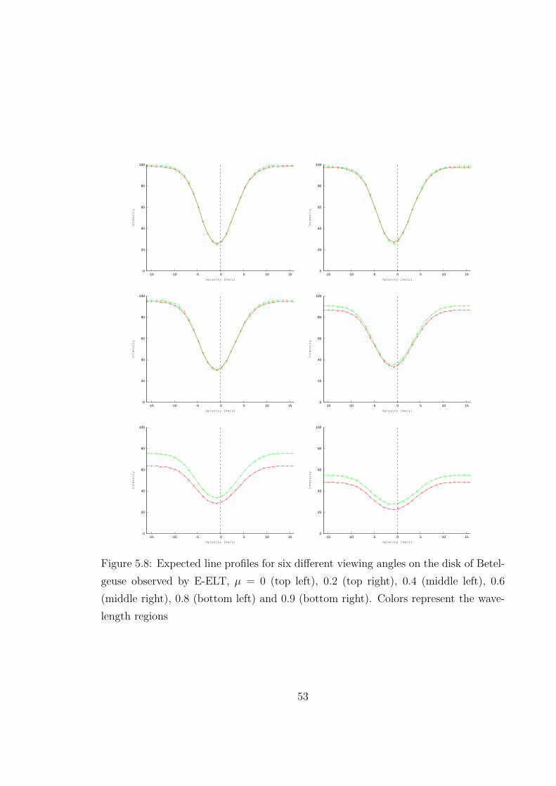
0

20

40

60

80

100

-15 -10 -5 0 5 10 15

Intensity

Velocity [km/s]

0

20

40

60

80

100

-15 -10 -5 0 5 10 15

Intensity

Velocity [km/s]

0

20

40

60

80

100

-15 -10 -5 0 5 10 15

Intensity

Velocity [km/s]

0

20

40

60

80

100

-15 -10 -5 0 5 10 15

Intensity

Velocity [km/s]

0

20

40

60

80

100

-15 -10 -5 0 5 10 15

Intensity

Velocity [km/s]

0

20

40

60

80

100

-15 -10 -5 0 5 10 15

Intensity

Velocity [km/s]

Figure 5.8: Expected line profiles for six different viewing angles on the disk of Betel-

geuse observed by E-ELT, µ = 0 (top left), 0.2 (top right), 0.4 (middle left), 0.6

(middle right), 0.8 (bottom left) and 0.9 (bottom right). Colors represent the wave-

length regions

53

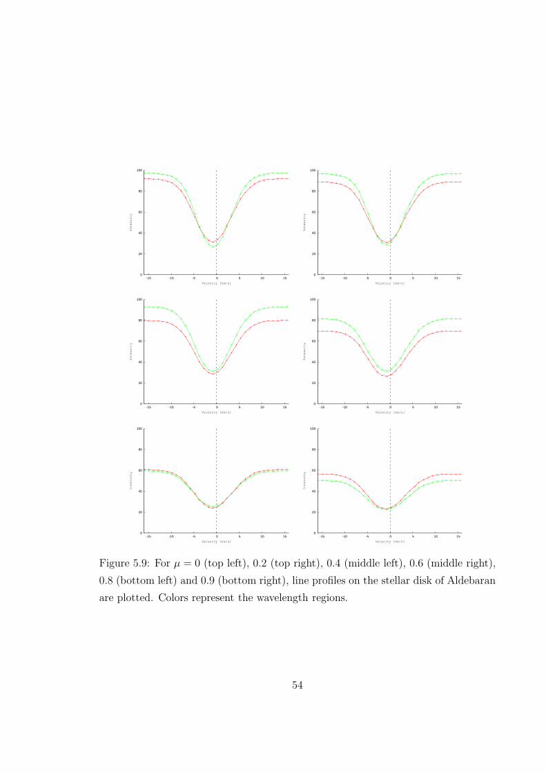
0

20

40

60

80

100

-15 -10 -5 0 5 10 15

Intensity

Velocity [km/s]

0

20

40

60

80

100

-15 -10 -5 0 5 10 15

Intensity

Velocity [km/s]

0

20

40

60

80

100

-15 -10 -5 0 5 10 15

Intensity

Velocity [km/s]

0

20

40

60

80

100

-15 -10 -5 0 5 10 15

Intensity

Velocity [km/s]

0

20

40

60

80

100

-15 -10 -5 0 5 10 15

Intensity

Velocity [km/s]

0

20

40

60

80

100

-15 -10 -5 0 5 10 15

Intensity

Velocity [km/s]

Figure 5.9: For µ = 0 (top left), 0.2 (top right), 0.4 (middle left), 0.6 (middle right),

0.8 (bottom left) and 0.9 (bottom right), line profiles on the stellar disk of Aldebaran

are plotted. Colors represent the wavelength regions.

54

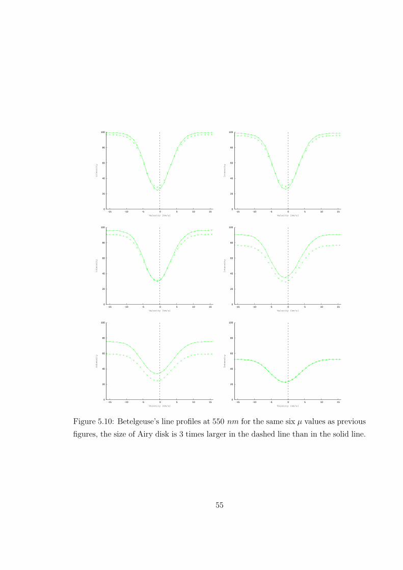
0

20

40

60

80

100

-15 -10 -5 0 5 10 15

Intensity

Velocity [km/s]

0

20

40

60

80

100

-15 -10 -5 0 5 10 15

Intensity

Velocity [km/s]

0

20

40

60

80

100

-15 -10 -5 0 5 10 15

Intensity

Velocity [km/s]

0

20

40

60

80

100

-15 -10 -5 0 5 10 15

Intensity

Velocity [km/s]

0

20

40

60

80

100

-15 -10 -5 0 5 10 15

Intensity

Velocity [km/s]

0

20

40

60

80

100

-15 -10 -5 0 5 10 15

Intensity

Velocity [km/s]

Figure 5.10: Betelgeuse’s line profiles at 550 nm for the same six µ values as previous

figures, the size of Airy disk is 3 times larger in the dashed line than in the solid line.

55

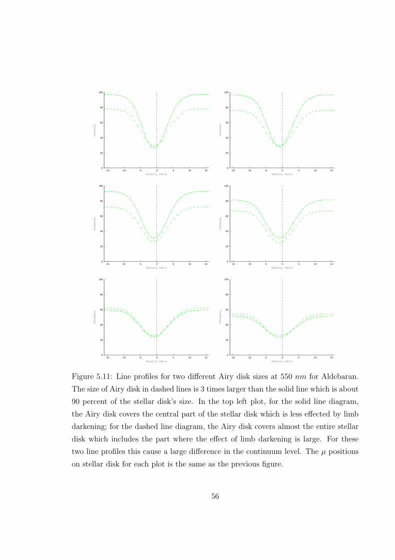
0

20

40

60

80

100

-15 -10 -5 0 5 10 15

Intensity

Velocity [km/s]

0

20

40

60

80

100

-15 -10 -5 0 5 10 15

Intensity

Velocity [km/s]

0

20

40

60

80

100

-15 -10 -5 0 5 10 15

Intensity

Velocity [km/s]

0

20

40

60

80

100

-15 -10 -5 0 5 10 15

Intensity

Velocity [km/s]

0

20

40

60

80

100

-15 -10 -5 0 5 10 15

Intensity

Velocity [km/s]

0

20

40

60

80

100

-15 -10 -5 0 5 10 15

Intensity

Velocity [km/s]

Figure 5.11: Line profiles for two different Airy disk sizes at 550 nm for Aldebaran.

The size of Airy disk in dashed lines is 3 times larger than the solid line which is about

90 percent of the stellar disk’s size. In the top left plot, for the solid line diagram,

the Airy disk covers the central part of the stellar disk which is less effected by limb

darkening; for the dashed line diagram, the Airy disk covers almost the entire stellar

disk which includes the part where the effect of limb darkening is large. For these

two line profiles this cause a large difference in the continuum level. The µ positions

on stellar disk for each plot is the same as the previous figure.

56

Chapter 6

Conclusion

In this chapter we are looking through what can be concluded from this project.

It is possible to measure the spectrum of part of stellar disk of low-temperature

dwarf main sequence stars during the planetary transits by measuring the spectrum of

star before/after the transit, and during different phases of transit. The subtraction

of these two spectra provides would be the spectrum of that part of stellar disk that

is hidden behind the planet at each phase. The optimum cases are systems of dwarf

stars with Jupiter-size planets. In these systems the ratio of the surface of the star to

the surface of the planet is about 0.01. This value is small enough to see the variation

of spectrum in different part of stellar disk, and it is also large enough for detecting

the signal of the part behind the planet.

Since the signal of the part hidden behind the planet is only about one percent of

stellar flux, the signal to noise ratio has to be high. However the exposure times must

be short due to the short time of duration of the transit. Still, for bright stars, it is

possible to get SNR of 300 in one exposure. One way to increase the SNR is to add

uncorrelated signals together. In this case we can add different line profiles of some

chemical element with closely similar characteristics such as comparable excitation

potential and line depth. This method would increase the SNR, by square root of

number of the lines.

In addition to use the ”indirect” method applicable to dwarf stars, for the other

end of stellar size range, giants and supergiants, a ”direct” method via interferometers

or extremely large telescope can be used to measure the spectrum of part of stellar

57

disks. Current instruments are beginning to resolve the angular sizes of stars, and

several have been measured.

The largest telescope in near future, European extremely large telescope, planed

to have a diameter 39 m. Assuming its adaptive optics work to their full extend, the

resolving power reaching to the diffraction limit would enable to resolve the disk of

stars larger than 7 mas with this telescope at 1 µm. For stars with angular size com-

parable to that of the supergiant Betelgeuse, the measurements would be acceptable

even if the adaptive optics produce an image size 3 times larger than the diffraction

limit. However to get reasonable measurements for stars with angular size compa-

rable to that of the giant Aldebaran, the adaptive optics must perform close to the

diffraction limit.

58

Bibliography

[1] M. Asplund, A. Nordlund, R. Trampedach, C. Allende Prieto, and R. F. Stein.

Line formation in solar granulation. I. Fe line shapes, shifts and asymmetries.

A&A, 359:729, July 2000.

[2] T. S. Boyajian, K. von Braun, G. van Belle, H. A. McAlister, T. A. ten Brum-

melaar, S. R. Kane, P. Muirhead, J. Jones, R. White, G. Schaefer, D. Ciardi,

T. Henry, M. Lopez-Morales, S. Ridgway, D. Gies, W.-C. Jao, B. Rojas-Ayala,

J. R. Parks, L. Sturmann, J. Sturmann, N. H. Turner, C. Farrington, P. J.

Goldfinger, and D. H. Berger. Stellar Diameters and Temperatures II. Main

Sequence K & M Stars. A&A ArXiv e-prints, Aug. 2012.

[3] M. Cagnet, M. Francon, J. C. Thrierr. Atlas optischer Erscheinungen. Springer,

1962.

[4] F. R. Chromey. To Measure the Sky An Introduction to Observational Astron-

omy. Cambridge University Press, first edition, 2010.

[5] M. J. Creech-Eakman, V. Romero, I. Payne, C. Haniff, D. Buscher, C. Aitken,

C. Anderson, E. Bakker, T. Coleman, C. Dahl, A. Farris, S. Jiminez, C. Jurgen-

son, R. King, D. Klinglesmith, III, K. McCord, T. McCracken, K. Nyland, A. Oli-

vares, M. Richmond, M. Romero, C. Salcido, J. Sandoval, F. Santoro, J. Sea-

mons, R. Selina, A. Shtromberg, J. Steenson, N. Torres, D. Westpfahl, F. Baron,

M. Fisher, E. Seneta, X. Sun, D. Wilson, and J. Young. Magdalena Ridge

Observatory Interferometer: advancing to first light and new science. (SPIE)

Conference Series, 7734, July 2010.

59

[6] D. Dravins. High-fidelity spectroscopy at the highest resolutions. Astronomische

Nachrichten, 331:535, May 2010.

[7] D. Dravins and A. Nordlund. Stellar Granulation - Part Five - Synthetic Spectral

Lines in Disk Integrated Starlight. A&A, 228:203, Feb. 1990.

[8] D. Dravins and A. Nordlund. Stellar Granulation - Part Four - Line Formation

in Inhomogeneous Stellar Photospheres. A&A, 228:184, Feb. 1990.

[9] B. Edlen. The identification of the coronal lines (George Darwin Lecture).

Monthly Not. Royal Astron. Soc., 105:323, 1945.

[10] J. Fraunhoffer. bla. Denkschriften der Koniglichen Akademie der Wissenschaften

zu Munchen fur das Jahre, 5:193, 1817.

[11] R. A. Freedman, R. M. Geller, and W. J. Kaufmann III. Universe. Cambridge

University Press, ninth edition, 2011.

[12] B. Freytag. Hot Spots in Numerical Simulations of Betelgeuse. The Future of

Cool-Star Astrophysics: 12th Cambridge Workshop on Cool Stars, Stellar Sys-

tems, and the Sun, 12:1024, Oct. 2003.

[13] D. F. Gray. The Observation and Analysis of Stellar Photospheres. Cambridge

University Press, third edition, 2008.

[14] G. E. Hale, F. Ellerman, S. B. Nicholson, and A. H. Joy. The Magnetic Polarity

of Sun-Spots. ApJ, 49:153, Apr. 1919.

[15] J. R. Holt. Spectroscopic Determination of Stellar Rotation. Astronomy and

Astro-Physics, 12:646, Aug. 1893.

[16] M. Hoskin. The Cambridge Illustrated History of Astronomy. Cambridge Uni-

versity Press, first edition, 1997.

[17] P. Kervella, T. Verhoelst, S. T. Ridgway, G. Perrin, S. Lacour, J. Cami, and

X. Haubois. The close circumstellar environment of Betelgeuse. Adaptive optics

spectro-imaging in the near-IR with VLT/NACO. A&A, 504:115, Sept. 2009.

60

[18] H.-G. Ludwig, E. Caffau, M. Steffen, B. Freytag, P. Bonifacio, and A. Kucinskas.

The CIFIST 3D model atmosphere grid. Mem.S.A.It., 80:711, 2009.

[19] D. B. McLaughlin. Some results of a spectrographic study of the Algol system.

ApJ, 60:22, July 1924.

[20] A. A. Michelson and F. G. Pease. Measurement of the diameter of alpha Orionis

with the interferometer. ApJ, 53:249, May 1921.

[21] D. J. Mullan. Physics of the Sun: A First Course. Chapman & Hall CRC,

Taylor & Francis group, first edition, 2010.

[22] D. Queloz, A. Eggenberger, M. Mayor, C. Perrier, J. L. Beuzit, D. Naef, J. P.

Sivan, and S. Udry. Detection of a spectroscopic transit by the planet orbiting

the star HD209458. A&A, 359:L13, July 2000.

[23] A. Richichi and V. Roccatagliata. Aldebaran’s angular diameter: How well do

we know it? A&A, 433:305, Apr. 2005.

[24] S. Ridgway. The Future of Ground-Based Optical Interferometry. Bulletin of

the American Astronomical Society, 37:1313, Dec. 2005.

[25] S. Rosseland. Viscosity in the stars. Monthly Not. Royal Astron. Soc., 89:49,

Nov. 1928.

[26] R. A. Rossiter. On the detection of an effect of rotation during eclipse in the

velocity of the brigher component of beta Lyrae, and on the constancy of velocity

of this system. ApJ, 60:15, July 1924.

[27] R. J. Rutten. Radiative Transfer in Stellar Atmospheres. http:

//www.staff.science.uu.nl/~rutte101/rrweb/rjr-edu/coursenotes/

rutten_rtsa_notes_2003.pdf, May 2003.

[28] H. C. van de Hulst. The electron density of the solar corona. Bulletin Astron.

Inst. Netherlands, 11:135, Feb. 1950.

[29] W. van Hamme. New limb-darkening coefficients for modeling binary star light

curves. AJ, 106:2096, Nov. 1993.

61

[30] J. V. Wall and C. R. Jenkins. Practical Statistics for Astronomers. Cambridge

University Press, third edition, 2008.

[31] S. Wedemeyer-Bohm. Dynamic models of the sun from the convection zone to

the chromosphere. IAU Symposium, 239:52, May 2007.

[32] J. S. Young, J. E. Baldwin, R. C. Boysen, C. A. Haniff, P. R. Lawson, C. D.

Mackay, D. Pearson, J. Rogers, D. St.-Jacques, P. J. Warner, D. M. A. Wilson,

and R. W. Wilson. New views of Betelgeuse: multi-wavelength surface imaging

and implications for models of hotspot generation. Monthly Not. Royal Astron.

Soc., 315:635, July 2000.

62