Spectrometry: Quantitative Determination of ASA by ... · PDF fileThis Experiment is a 3 hour Analytical Chemistry ... The beneficial properties of salicylic acid ... (Ethanoic Acid)

CHEMICAL, ENVIRONMENTAL, AND BIOTECHNOLOGY DEPARTMENT

Spectrometry: Quantitative Determination of ASA by

Absorbance of Visible Light

by Professor David Cash

September, 2008

Mohawk College is the author and owner of these materials (excluding copyright held by others) and all copyright and

intellectual property rights contained therein.

Use of these materials for teaching or other non-commercial purposes is allowed.

Contact information for Mohawk College will be found on

the following page.

This Experiment is a 3 hour Analytical Chemistry laboratory exercise. It is designed for students in a common

second term course of a 2-year diploma program (Biotechnology, Environmental, or Health Technician).

For Information or Assistance

Contact:

MOHAWK COLLEGE CHEMICAL, ENVIRONMENTAL, AND

BIOTECHNOLOGY DEPARTMENT

Professor Cindy Mehlenbacher [email protected]

905-575-1212 ext. 3122

Bill Rolfe (Chief Technologist) [email protected]

905-575-2234

1

Experiment 8

Spectrophotometry:

Analysis of the ASA content of a Tablet by Use of the Beer-Lambert Law

OBJECTIVE A spectrophotometric analysis will be performed. The comprehension and skills learned will be transferable to other laboratory and workplace situations. • A set of ASA solution standards will be prepared; the photometric absorbances of the

solution standards at 530 nm wavelength will be used to construct a least squares linear calibration curve.

• The calibration curve will be used to estimate the ASA content of an ASA tablet unknown. REFERENCE Harris, Chapter 4, pages 79-85 and Chapter 18, pages 378-390. INTRODUCTION Spectrophotometry This method of analysis, sometimes called spectrometry, refers to a method based on the measurement (metry) of light energy (photo) at a selected wavelength (spectro). Harris (Chapter 18) gives an introduction to the theory and practice of spectrometry. What follows is a practical introduction to using molecular absorption spectrometry in an analysis. Molecular Absorption Spectrometry Some molecular substances and some polyatomic ions in solution absorb ultraviolet, visible, or infrared light energy. The amount of the absorption of the light varies with the substance, with the selected wavelength of the light, and with the temperature.

2

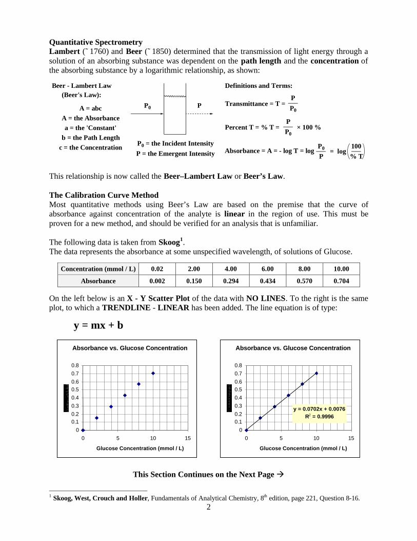
Quantitative Spectrometry Lambert (˜ 1760) and Beer (˜ 1850) determined that the transmission of light energy through a solution of an absorbing substance was dependent on the path length and the concentration of the absorbing substance by a logarithmic relationship, as shown:

P0 P

Definitions and Terms:

Transmittance = T =PP0

PP0

Percent T = % T = × 100 %b = the Path Length

c = the Concentration

Beer - Lambert Law(Beer's Law):

A = abc

a = the 'Constant'A = the Absorbance

P0 = the Incident IntensityP = the Emergent Intensity Absorbance = A = - log T = log

P0

P100% T

= log

This relationship is now called the Beer–Lambert Law or Beer’s Law. The Calibration Curve Method Most quantitative methods using Beer’s Law are based on the premise that the curve of absorbance against concentration of the analyte is linear in the region of use. This must be proven for a new method, and should be verified for an analysis that is unfamiliar. The following data is taken from Skoog1. The data represents the absorbance at some unspecified wavelength, of solutions of Glucose.

Concentration (mmol / L) 0.02 2.00 4.00 6.00 8.00 10.00

Absorbance 0.002 0.150 0.294 0.434 0.570 0.704

On the left below is an X - Y Scatter Plot of the data with NO LINES. To the right is the same plot, to which a TRENDLINE - LINEAR has been added. The line equation is of type:

y = mx + b

This Section Continues on the Next Page à

1 Skoog, West, Crouch and Holler, Fundamentals of Analytical Chemistry, 8th edition, page 221, Question 8-16.

Absorbance vs. Glucose Concentration

y = 0.0702x + 0.0076 R 2 = 0.9996

0 0.1 0.2 0.3 0.4 0.5 0.6 0.7 0.8

0 5 10 15 Glucose Concentration (mmol / L)

Absorbance vs. Glucose Concentration

0 0.1 0.2 0.3 0.4 0.5 0.6 0.7 0.8

0 5 10 15 Glucose Concentration (mmol / L)

3

The Calibration Curve Method (Cont.) The equation of the line and the R2 value are displayed on the plot. The closer the value of R2 is to 1.0000, the better the fit of the data is to a straight line. For this particular set of data the slope and intercept value of the linear trendline are very small numbers. In such a case, when the equation is displayed and selected, it is necessary to format the numbers in the equation to be displayed to a chosen number of decimal places. In this case, four (4) decimal places has been chosen. Using Beer’s Law in Analysis Beer’s Law can be used in an analysis in many ways. Starting from the best possible method: 1. The best way is to prepare a calibration curve from a set of independently prepared

calibration standard solutions. This means each calibration solution is prepared from a separate weighing operation. Solutions of unknowns will have their concentration determined by using the calibration curve equation.

2. The second best way is to prepare a calibration curve from a set of calibration standard

solutions prepared from a single stock solution. Solutions of unknowns will have their concentration determined by using the calibration curve equation. This method will fail if the stock solution is not properly prepared or if the dilutions are faulty, but this may not be immediately apparent. This is a normal method for experienced analysts, since all mass values and dilutions are assumed to be reliable, and quality assurance protocols are usually in effect to detect any problems in methodology.

3. A slightly less reliable method is standard addition. A known amount of analyte is added

into the unknown solution. The absorbance is measured with and without the addition. This can work well if you are certain that you are in a linear region of the calibration curve.

4. The least reliable method is by proportion. The absorbance of the unknown solution is

related to the absorbance of a single calibration standard solution. This can work well if you are certain that you are in a linear region of the calibration curve. In this method, the following relationship is utilized:

Concentration of Unknown

Concentration of Standard

Absorbance of Unknown

Absorbance of Standard=

4

Uncertainty in Using a Calibration Curve Method Skoog (8th edition, pages 207-208) discusses the uncertainty of using a calibration curve method in detail. Harris covers most of the same points without being as explicit. The uncertainty of the slope and intercept values lead to increasing uncertainty at the outer ends of the calibration region. When using a calibration curve with a linear trendline, always keep the unknowns at the centre of the linear calibration curve range. Precision and Accuracy in Spectrophotometry Harris discusses the precision and accuracy of using a spectrophotometer (page 385) and advises keeping the Absorbance of the solutions between the values 0.4 and 0.9. Skoog , 8th Edition gives a more detailed discussion (Figure 26-11, page 801); the accuracy and precision of every instrument is different. A Spectronic 20, the type of instrument you will probably use, is accurate and precise to within 2 % over the range of Absorbance from about 0.2 to 0.9. More expensive instruments can be accurate and precise to within 1 % or better over a range of Absorbance from 0.1 to 2.0 or greater. Constraints on a Beer’s Law Analysis To use Beer’s Law in analysis successfully, some caution is required. • Keep the temperature constant (room temperature is usually used). • Keep the wavelength fixed, and as narrow a range as possible.

This depends on the nature and quality of the instrument used. • Keep the cell path length constant (use the same cell for all measurements). • Keep solutions free of dust or other solids, which block or scatter the transmission of light. • Keep the cell surface clean, and free of dirt, grease, and scratches. • The absorbance curve may have a limited linear range of concentrations.

Keep to the linear range. • Instrument error increases at very low absorbance and at very high absorbance.

This depends on the instrument. See Harris, Figure 18-8, page 385. Keep to the middle range of absorbances (0.2 – 0.9) for all analysis solutions.

• Check for interference. If there is some other substance present that absorbs at the same wavelength, called a ‘matrix’ effect, this will increase error greatly. Check for background absorbance at the analytical wavelength.

5

Acetylsalicylic Acid The beneficial properties of salicylic acid (2-hydroxybenzoic acid) have probably been known to human beings for many tens of thousands of years. This compound, widely found in nature in the roots, bark, leaves and fruits of many plants and trees, is an analgesic (relieves pain), an antipyretic (reduces fever) and an anti-inflammatory (reduces swelling). It can be taken orally (by mouth), but is very acidic and irritates the stomach lining severely. The compound acetylsalicylic acid, also known as ASA or Aspirin®, was first synthesized in 1853. This compound breaks down rapidly in the body to form salicylic acid, giving all the same beneficial effects as salicylic acid, but it can be taken orally with far less irritation of the stomach. Acetylsalicylic acid is a solid at room temperature, existing as a white powder or white crystalline needles2. It has a melting point of 135 – 137 ºC, and decomposes at 140 ºC. It is not very soluble in water, about 0.33 g / 100 mL at 25 ºC, but is much more soluble in alcohols and acetone. Both salicylic acid and ASA are toxic and can be fatal in excess. The LD50

3 for acetylsalicylic acid4 in rats is about 200 mg / kg. The LD50 for salicylic acid5 in rats is about 900 mg / kg. Synthesis of Acetylsalicylic Acid The commercial synthesis of acetylsalicylic acid utilizes the reaction of salicylic acid with acetic anhydride, using acid catalysis as shown in the equation below. The byproduct acetic acid is also recovered and reused.

CO OH

OHH

HH

H

CCH3

O

OCCH3

O

+

H+

catalyst

CO OH

OCO

CH3H

HH

H

CCH3

O

OH+

Salicylic Acid (2-Hydroxybenzoic acid) C7H6O3 = 138.12 g / mol

Acetic Anhydride 102.09 g / mol Acetylsalicylic Acid

C9H8O4 = 180.17 g / mol

Acetic Acid (Ethanoic Acid)

60.05 g / mol

ASA as a Carboxylic Acid Since ASA is a carboxylic acid, it acts as a weak acid and can be neutralized by an alkali to form a salt. The Ka value of ASA is 3.3 × 10-4.

+

CO OH

OCO

CH3H2O

H

HH

H

CO O

OCO

CH3H

HH

H

+ H3O+ K = Ka

2 Merck Index, 9th Edition, 1976, Merck and Co., Entry 874, page 114. 3 LD50 (lethal dose 50 %): the amount of a toxic agent (as a poison, virus, or radiation) that is sufficient to kill 50 percent of a population of animals usually within a certain time. 4 http://www2.siri.org/msds/f2/cfg/cfgqj.html (retrieved 2006 06 08) 5 https://fscimage.fishersci.com/msds/20315.htm (retrieved 2006 06 08)

6

Stability of Acetylsalicylic Acid Acetylsalicylic acid is not chemically inert. If exposed to moisture, over time it breaks down to form salicylic acid and acetic acid. A sealed bottle of ASA tablets that is kept past its expiry date will often have an odour of acetic acid (vinegar) when opened:

CO OH

OH+ +

CO OH

OCO

CH3CCH3

O

OHH2O

H

HH

H

H

HH

H

The breakdown of ASA is much more rapid in the presence of acid or base, and at higher temperature. Bottles of low-dose ASA usually contain a small canister of silica gel mixed with activated carbon. The silica gel absorbs water vapour, and the activated carbon absorbs acetic acid vapour. Solubility Considerations ASA is not very soluble in water. Also, solid crystals of ASA are very slow to dissolve at room temperature. The ASA in tablets for human consumption are in the form of a very fine powder. The powdered ASA dissolves much more rapidly than large crystals of solid. Tablet Coatings and Binders ASA tablets sold as over-the-counter medications may have two kinds of coatings. Most tablets have a coating that makes them easy to swallow, but disintegrates rapidly in water. Some tablets are enteric6 coated. The enteric coating does not dissolve rapidly in the acidic solution present in the stomach, but does dissolve or soften in the neutral or slightly basic solution present in the small intestine. An enteric coating is used to prevent exposure of the stomach or esophagus to ASA. Some people find ASA to be a very irritating and dangerous drug. The enteric coating on an ASA tablet is usually a polymeric substance. Although it softens and allows the powder inside to escape, it does not fully dissolve. Most tablets contain binder substances, which hold the powdered material into a pill shape. Starch is often used as a binder. The binders are usually insoluble in water. Coating and binder substances can be removed by a filtration step, to prevent interference with the analytical measurements.

6 Merriam-Webster Dictionary: enteric - being a coating (as of an aspirin tablet) designed to pass through the stomach unaltered and disintegrate in the intestines.

7

Analysis of ASA by Spectrometry The analysis of ASA by spectrometry is actually the analysis of salicylic acid by spectrometry. Acetylsalicylic acid (ASA) is rapidly decomposed to salicylic acid by boiling in sodium hydroxide solution. It is a convenient fiction in the analysis to calculate solution concentrations as if the ASA were still present

CO OH

OCO

CH3H

HH

H

+ H2O NaOH

heat

CO OH

OHH

HH

H

+ CCH3

O

OH

Acetylsalicylic Acid Salicylic Acid Acetic Acid

Formation of the Ferric Ion Complex of Salicylic Acid Ferric ion is well known for its ability to form intensely coloured complexes with phenols. This reaction is characteristic of almost all phenols, including salicylic acid. This reaction is used as a test for the presence of a phenol.

Complex Ion formed by Salicylic Acid and Ferric Ion The complex ion formed may not be exactly as shown here. The unlabeled positions around the ferric ion are probably occupied by the oxygen atoms of water molecules. Regardless, in water solution, in the presence of an excess of ferric ions, salicylic acid reacts quantitatively to form an intensely coloured substance. To the human eye, the solution appears to be purple-violet in colour. A maximum of absorbance of visible light by the complex ion occurs at a wavelength of 530 nm. This is the wavelength which should be selected for photometry.

Wavelength Scan of the Ferric Ion – Salicylate Complex

Absorbance versus Wavelength

for a Calibration Standard Solution

Note the Absorbance Maximum at about 530 nm Wavelength

Scan Obtained on a NovaSpec Plus

Diode Array Spectrophotometer (2008 03 13)

330nm 400nm 500nm 600nm 700nm 800nm0.0A

0.1A

0.2A

0.3A

0.4A

0.5A Wavelength Scan

CO

H

H

H H

Fe

O

O

8

An Example Data Set and an Example of a Calibration Curve for the Experiment A single sample of pure ASA was weighed out using an analytical balance, heated in 1.0 M NaOH solution, and diluted with distilled water into a 250 mL volumetric flask to form a stock solution. Portions of this stock solution of ASA were measured out from a buret into a set of five (5) 50 mL volumetric flasks. This is Method 2 on page 3. The solutions were all diluted to 50 mL total volume with a solution of 0.02 M ferric ion in 0.1 M HCl solution. This latter solution was used as a blank or background to zero the instrument. All of the solution standards were violet – purple to the human eye. The absorbance of each solution was measured in duplicate at 530 nm wavelength on a Spectronic 20 instrument, using the same 1 cm path-length test tube cell for all measurements. The Table below gives the concentration and the mean absorbance of each of the five calibration solution standards as though the ASA were still present, a convenient fiction. The concentrations are given in mg / L units, also called ppm or parts per million units. An Excel X – Y Scatter plot of this data, the best-fit least-squares linear trendline, the line equation, and the R2 value are shown. For the data set of this experiment, it will be necessary to choose to display the slope and intercept values of the trendline equation to five (5) places after the decimal point.

ASA Conc. (mg / L)

Mean Absorbance

15.9 0.097

31.8 0.192

48.4 0.292

65.6 0.396

84.0 0.508

Absorbance at 530 nm vs. ASA Concentration (ppm)

y = 0.00604x + 0.00040R2 = 0.99999

0

0.1

0.2

0.3

0.4

0.5

0.6

0 10 20 30 40 50 60 70 80 90

ASA Concentration (mg / L = ppm)

Ab

sorb

ance

9

Dilution Dilution is a technical term used in the laboratory when the volume of a solution is increased. To dilute means to add solvent to increase the volume of a solution, so that the concentration of the solution goes from a higher value to a lower value. Dilution is used very often in the laboratory. Many reagents are purchased as highly concentrated solutions which must be reduced in concentration for daily use. In instrumental analysis, solutions of very low concentration are often required as standards of comparison. These are made by dilution of standard solutions. Dilution of reagent solutions used in excess or approximate quantity may be done approximately, using graduated cylinders and beakers. Standard solutions must be diluted as accurately and precisely as possible, using volumetric apparatus. Simple Dilution The most common dilution is the single step or simple dilution. The calculation of a simple dilution procedure is done using the dilution equation:

Cdilute × Vdilute = Cconcentrated × Vconcentrated This looks like the equation of a titration, because both sides represent a quantity. That quantity is the amount of dissolved substance, which does not change on dilution. So there is no balanced equation or mol to mol ratio to worry about in a dilution. The dilution equation may be rewritten in terms of ratios:

VconcentratedCdilute

VdiluteCconcentrated=

It may also be written in terms of a dilution factor:


Vdilute

Cconcentrated= ×DilutionFactor

When the volume of a solution is increased by a certain factor, say 10 mL to 50 mL, this is referred to as a 1 to 5 dilution or a five-fold dilution. In this case, the new concentration (Cdilute) is 1 / 5 of the old concentration (Cconcentrated). Always use your chemical common sense to check the result of a dilution calculation. (Does it compute?) Notice that you can use any concentration unit in a dilution calculation and any volume unit, as long as you do not change the units during the calculation.

10

Serial Dilution In a serial dilution, one dilution follows another. Serial dilution makes it easy to prepare solutions of very low concentration. For example: A stock standard solution of zinc chloride contains 1100 ppm (mg / L) zinc ion. An intermediate standard solution is prepared by diluting 10.00 mL of the stock solution to 100.0 mL in a volumetric flask. A working standard solution is prepared by diluting 5.00 mL of the intermediate standard solution to 100.0 mL volume. What is the concentration of each of the diluted solutions?

A Stock Solution of Zinc in

Water (1100 mg / L) First Dilution 10 to 100

(1 to 10) Second Dilution 5 to 100

(1 to 20)

1100 mg / L 110 mg / L 5.5 mg / L

The calculation can be done in two steps, each a simple dilution. It can also be done in one step for the final solution by multiplying the dilution factors together and using the ratio equation:


Vdilute

Cconcentrated= ×

In the above dilution scheme, the overall dilution factor is (1 / 10) × (1 / 20) = (1 / 200). Multiple Dilution This is a procedure carried out when a range of standard comparison solutions is needed for an analysis. In the example above, a set of solutions might have been prepared by taking 1.00, 2.00, 3.00, 4.00 and 5.00 mL of the intermediate standard solution and diluting each portion to 100 mL. The working standard solutions would be 1.10 ppm, 2.20 ppm, 3.30 ppm, 4.40 ppm and 5.50 ppm zinc respectively.

Intermediate

Standard Solution

Dilution of 1.00 mL to

100 mL (1 to 100)


100 mL (2 to 100)


100 mL (3 to 100)


100 mL (4 to 100)


100 mL (5 to 100)

110 mg / L 1.10 mg / L 2.20 mg / L 3.30 mg / L 4.40 mg / L 5.50 mg / L

11

Sample Calculations Preparation of a Stock Standard Solution of ASA Example 1 A precisely weighed sample of 0.2018 g of analytical-grade pure solid ASA was boiled in 1.0 M NaOH solution, following the instructions of this experiment. The resulting solution was washed quantitatively into a 250 mL (0.2500 L) volumetric flask, diluted to volume with distilled water, and mixed completely. The resulting solution was a stock standard solution of ASA. Calculate the concentration of the ASA in the stock standard solution in mg / L (ppm) units. State the value to 4 significant figures. Answer Use the definition of concentration in mg / L (ppm):

Concentration in mg / L (ppm) =

Mass Solute (mg)

Volume Solution (L)

Concentration in mg / L (ppm) =

1000 mg

1 g0.2018 g × ×

1

0.2500 L

Concentration of ASA = 807.2 mg / L (ppm)

Preparation of a Diluted Solution of Standard ASA Example 2 A 4.00 mL sample of the stock standard solution of ASA of Example 1 was pipetted into a 50.00 mL volumetric flask and diluted to volume with 0.02 M ferric ion solution in 0.1 M HCl solution. This is a diluted standard solution of ASA for a calibration curve. Calculate the concentration of the ASA in the diluted standard solution in mg / L (ppm) units. State the value to 3 significant figures. Answer Use the dilution relationship:


Vdilute

Cconcentrated= × 807.2 mg / L (ppm)=4.00 mL

50.00 mL×

Concentration of Diluted ASA = 64.6 mg / L (ppm)

The Sample Calculations Section Continues on the Next Page à

12

Sample Calculations (Cont.) Use of a Calibration Curve An ASA tablet, nominal ASA content 325 mg, was boiled in 1.0 M NaOH solution, following the instructions of this experiment. The resulting mixture was filtered and washed quantitatively into a 250 mL (0.2500 L) volumetric flask and diluted to volume with distilled water. The resulting solution is the stock solution of the tablet unknown. A 2.00 mL sample of the stock solution of the tablet unknown was pipetted into a 50.00 mL volumetric flask and diluted to volume with 0.02 M ferric ion solution in 0.1 M HCl solution. This is the diluted solution of the tablet unknown. The absorbance of this solution was meaured on the same instrument as for the calibration data and curve on page 8, using the same test tube sample cell, at the same time, without changing the wavelength setting.

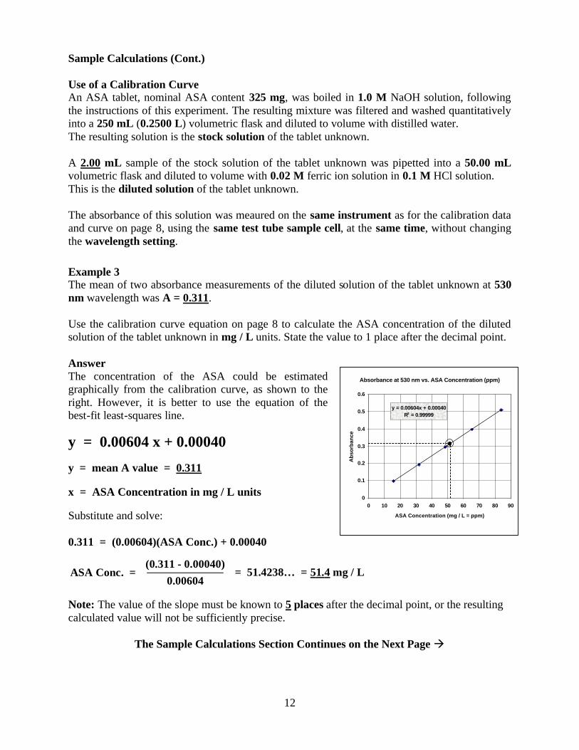
Example 3 The mean of two absorbance measurements of the diluted solution of the tablet unknown at 530 nm wavelength was A = 0.311. Use the calibration curve equation on page 8 to calculate the ASA concentration of the diluted solution of the tablet unknown in mg / L units. State the value to 1 place after the decimal point. Answer The concentration of the ASA could be estimated graphically from the calibration curve, as shown to the right. However, it is better to use the equation of the best-fit least-squares line.

y = 0.00604 x + 0.00040 y = mean A value = 0.311 x = ASA Concentration in mg / L units Substitute and solve: 0.311 = (0.00604)(ASA Conc.) + 0.00040

ASA Conc. =(0.311 - 0.00040)

0.00604= 51.4238… = 51.4 mg / L

Note: The value of the slope must be known to 5 places after the decimal point, or the resulting calculated value will not be sufficiently precise.


Absorbance at 530 nm vs. ASA Concentration (ppm)

y = 0.00604x + 0.00040R2 = 0.99999

0

0.1

0.2

0.3

0.4

0.5

0.6

0 10 20 30 40 50 60 70 80 90


Ab

sorb

ance

13

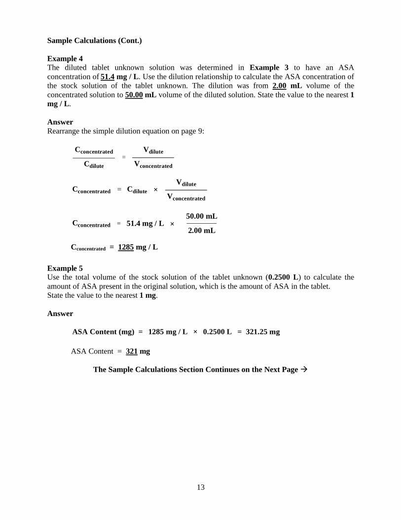
Sample Calculations (Cont.) Example 4 The diluted tablet unknown solution was determined in Example 3 to have an ASA concentration of 51.4 mg / L. Use the dilution relationship to calculate the ASA concentration of the stock solution of the tablet unknown. The dilution was from 2.00 mL volume of the concentrated solution to 50.00 mL volume of the diluted solution. State the value to the nearest 1 mg / L. Answer Rearrange the simple dilution equation on page 9:


VdiluteCconcentrated=

Vconcentrated

Cdilute

VdiluteCconcentrated = ×

2.00 mL51.4 mg / L

50.00 mLCconcentrated = ×

Cconcentrated = 1285 mg / L

Example 5 Use the total volume of the stock solution of the tablet unknown (0.2500 L) to calculate the amount of ASA present in the original solution, which is the amount of ASA in the tablet. State the value to the nearest 1 mg. Answer

1285 mg / L × 0.2500 L = 321.25 mgASA Content (mg) =

ASA Content = 321 mg


14

Sample Calculations (Cont.) Example 6 A weighed sample of analytical-grade ASA and an ASA tablet unknown were treated according to the experiment procedure. The data in the Table to the right were obtained. Calculate the ASA concentration in the diluted unknown solution by the method of proportion. State the value to the nearest 0.1 mg / L. Answer This is Method 4 on page 3. Rearrange the relationship as shown, substitute and solve:

Concentration of Unknown

Concentration of Standard


Absorbance of Standard=

Concentration of Unknown Concentration of Standard


Absorbance of Standard= ×

Concentration of Unknown 48.7 mg / L

0.314

0.295= ×

ASA Concentration in the Diluted Unknown Solution = 51.8366… = 51.8 mg / L

ASA Conc. (mg / L)

Mean Absorbance

48.7 0.295

Diluted Unknown 0.314

15

Name Day Start Time

PRE-LABORATORY PREPARATION To be completed before the laboratory session. To be submitted before beginning the experiment (20 points). Questions: Answer in the space provided. Show work.

Your Mohawk College ID Number is nnnnVWXYZ. Calibration Curve Exercise (7 points) Suppose that the data in the Table below were obtained by the method of this experiment. Use your Mohawk ID Number to determine and enter the value of each datum7.

ASA Conc. (mg / L)

ASA Conc. (mg / L)

Mean Absorbance

Mean Absorbance

15.V 0.09Z

31.W 0.19Y

48.X 0.29X

65.Y 0.39W

84.Z 0.50V

Instructions: a. Use a software package (e.g.: Microsoft Excel®) to display an X - Y Scatter Plot of the data.

Choose the no-lines option. b. Title the plot, including your name and the date, and label both axes. c. Choose a linear least-squares best-fit trendline to the data. d. Display the trendline on your plot and also display the equation and R2 value of the

trendline. e. Use the cursor to select the equation box.

Format as a number and choose the option five (5) places after the decimal point. f. Attach a print-out of your completed plot to the PRE-LABORATORY PREPARATION.

The PRE-LABORATORY PREPARATION Continues on the Next Page à

7 Datum (Merriam-Webster Dictionary) - something used as a basis for calculating or measuring. Plural: data or datums.

16

PRE-LABORATORY PREPARATION (Cont.) Preparation of a Stock Standard Solution of ASA A precisely weighed sample of 0.20XY g of analytical-grade pure solid ASA was boiled in 1.0 M NaOH solution, following the instructions of this experiment. The resulting solution was washed quantitatively into a 250 mL (0.2500 L) volumetric flask, diluted to volume with distilled water, and mixed completely. The resulting solution was a stock standard solution of ASA. Q-1. Calculate the concentration of the ASA in the stock standard solution in mg / L (ppm)

units. State the value to 4 significant figures. (2 points) Show work. See Example 1 on page 11.

0.20XY g = g

ASA Concentration of the Standard Stock Solution (mg / L) = mg / L

Preparation of a Diluted Solution of Standard ASA A 3.00 mL sample of the stock standard solution of ASA of Example 1 was pipetted into a 50.00 mL volumetric flask and diluted to volume with 0.02 M ferric ion solution in 0.1 M HCl solution. This is a diluted standard solution of ASA for a calibration curve. Q-2. Calculate the concentration of the ASA in the diluted standard solution in mg / L (ppm)

units. State the value to 3 significant figures. (2 points) Show work. See Example 2 on page 11.

ASA Concentration of the Diluted Stock Solution (mg / L) = mg / L


17

Name Day Start Time

PRE-LABORATORY PREPARATION (Cont.) Use of a Calibration Curve An ASA tablet, nominal ASA content 325 mg, was boiled in 1.0 M NaOH solution, following the instructions of this experiment. The resulting mixture was filtered and washed quantitatively into a 250 mL (0.2500 L) volumetric flask and diluted to volume with distilled water to prepare a stock solution. A 2.00 mL sample of the stock solution of the tablet unknown was pipetted into a 50.00 mL volumetric flask and diluted to volume with 0.02 M ferric ion solution in 0.1 M HCl solution. The mean of two absorbance measurements of the diluted solution of the tablet unknown at 530 nm wavelength was A = 0.31Z. Q-3. Use your calibration curve equation from the Calibration Curve Exercise to calculate

the ASA concentration of the diluted solution of the tablet unknown in mg / L units. State the value to 1 place after the decimal point. (5 points) Show work. See Example 3 on page 12.

A = 0.31Z =

ASA Conc. the Diluted Stock Solution of the Unknown (mg / L) = mg / L


18

PRE-LABORATORY PREPARATION (Cont.) Q-4. Use the dilution relationship to calculate the ASA concentration of the stock solution of

the tablet unknown. The dilution was from 2.00 mL volume of the concentrated solution to 50.00 mL volume of the diluted solution. (2 points) State the value to the nearest 1 mg / L. Show work. See Example 4 on page 13.

ASA Conc. of the Stock Solution of the Unknown (mg / L) = mg / L Q-5. Use the total volume of the stock solution of the tablet unknown (0.2500 L) to calculate

the total amount of ASA in the tablet. (2 points) State the value to the nearest 1 mg. Show work. See Example 5 on page 13.

Total ASA Content of the Tablet Unknown (mg) = mg

PRE-LABORATORY PREPARATION Total = / 20

19

PROCEDURE Ensure that the fume hood fans are switched ON and are operating. There are no special disposal instructions for this experiment. All solids and solutions may safely be disposed of by way of the municipal solid waste containers or the sinks. However, 1.0 M NaOH solution is moderately corrosive and hazardous, and must be used with caution and respect. A. Preparation of Glassware and Apparatus Work with a Partner You will be assigned to work with a partner on Parts A to E of the experiment. Record the name of your partner on page 33 in the DATA TABLES AND REPORT section. The data from three to five partnerships will be combined as a supergroup to produce a calibration curve for the analysis. The following clean glassware and laboratory apparatus is required for the experiment:

For each pair of students: 9 a spatula 9 a glass stirring rod 9 a long stem funnel 9 three small beakers 9 two erlenmeyer flasks

9 a weighing bottle and its lid* 9 two 250 mL volumetric flasks and their stoppers 9 two 50 mL volumetric flasks and their stoppers (extra equipment) 9 a 10 mL Mohr graduated pipet 9 a rubber pipet squeeze bulb

* The instructor may instead direct you to weigh the ASA using a clean, dry weighing boat. A-1. Clean the glassware and apparatus if necessary with a 1 % solution of detergent in warm

water. See Cleaning and Drying of Glassware on page Error! Bookmark not defined.. Rinse the cleaned glassware and apparatus with tap water and then with distilled water. To avoid breakage, do not leave any glassware standing in an unstable position.

A-2. Dry the spatula, and the weighing bottle and its lid (if using the weighing bottle) in the

oven at 110 or 120 ºC for 15 minutes. Carefully remove the spatula and the weighing bottle and its lid from the oven on to a heat proof pad, and allow them to cool to room temperature before using them.

A-3. The instructor will set up one or more hot-plates. Using large beakers, heat 25 mL of

distilled water per student for the filtration step in Part B. The filtration of Part B may be slow. Complete Part B as soon as possible.

20

Work with your Partner. Part B and Part C may be completed in sequence or simultaneously. B. ASA Unknown – Stock Solution Preparation B-1. Label your two erlenmeyer flasks, to avoid confusion or loss later in a crowd of similar

flasks. Label one to contain an ASA tablet unknown for analysis, and the other to contain a sample of analytical-grade ASA.

B-2. Record the brand of your assigned ASA tablet unknown sample in Table B. Record a

description of the tablet and the nominal ASA content (mg). Weigh the tablet accurately. Record the mass value in mg units in Table B. Place the tablet into its labeled flask.

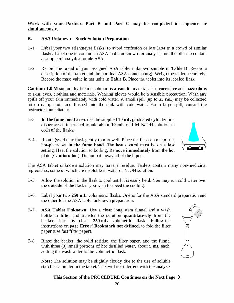
Caution: 1.0 M sodium hydroxide solution is a caustic material. It is corrosive and hazardous to skin, eyes, clothing and materials. Wearing gloves would be a sensible precaution. Wash any spills off your skin immediately with cold water. A small spill (up to 25 mL) may be collected into a damp cloth and flushed into the sink with cold water. For a large spill, consult the instructor immediately. B-3. In the fume hood area, use the supplied 10 mL graduated cylinder or a

dispenser as instructed to add about 10 mL of 1 M NaOH solution to each of the flasks.

B-4. Rotate (swirl) the flask gently to mix well. Place the flask on one of the

hot-plates set in the fume hood. The heat control must be on a low setting. Heat the solution to boiling. Remove immediately from the hot plate (Caution: hot). Do not boil away all of the liquid.

The ASA tablet unknown solution may have a residue. Tablets contain many non-medicinal ingredients, some of which are insoluble in water or NaOH solution. B-5. Allow the solution in the flask to cool until it is easily held. You may run cold water over

the outside of the flask if you wish to speed the cooling. B-6. Label your two 250 mL volumetric flasks. One is for the ASA standard preparation and

the other for the ASA tablet unknown preparation. B-7. ASA Tablet Unknown: Use a clean long stem funnel and a wash

bottle to filter and transfer the solution quantitatively from the beaker, into its clean 250 mL volumetric flask. Follow the instructions on page Error! Bookmark not defined. to fold the filter paper (use fast filter paper).

B-8. Rinse the beaker, the solid residue, the filter paper, and the funnel

with three (3) small portions of hot distilled water, about 5 mL each, adding the wash water to the volumetric flask.

Note: The solution may be slightly cloudy due to the use of soluble starch as a binder in the tablet. This will not interfere with the analysis.

This Section of the PROCEDURE Continues on the Next Page à

21

B. ASA Unknown – Stock Solution Preparation (Cont.) B-9. Add distilled water to the flask to about one cm below the mark line.

Fill the flask to the mark line using a dropper pipet. B-10. Stopper the flask with a clean stopper. Hold the stopper in place with one hand. Turn the

flask over slowly at least 17 times to ensure that the solution is completely uniform.

C. ASA Standard – Stock Solution Preparation C-1. If not already done, carefully remove the spatula and the weighing bottle and its lid

(if required) from the oven on to a heat proof pad, and allow them to cool to room temperature before using them.

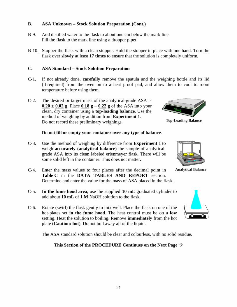
C-2. The desired or target mass of the analytical-grade ASA is

0.20 ± 0.02 g. Place 0.18 g – 0.22 g of the ASA into your clean, dry container using a top-loading balance. Use the method of weighing by addition from Experiment 1. Do not record these preliminary weighings.

Do not fill or empty your container over any type of balance. C-3. Use the method of weighing by difference from Experiment 1 to

weigh accurately (analytical balance) the sample of analytical-grade ASA into its clean labeled erlenmeyer flask. There will be some solid left in the container. This does not matter.

C-4. Enter the mass values to four places after the decimal point in

Table C in the DATA TABLES AND REPORT section. Determine and enter the value for the mass of ASA placed in the flask.

C-5. In the fume hood area, use the supplied 10 mL graduated cylinder to

add about 10 mL of 1 M NaOH solution to the flask. C-6. Rotate (swirl) the flask gently to mix well. Place the flask on one of the

hot-plates set in the fume hood. The heat control must be on a low setting. Heat the solution to boiling. Remove immediately from the hot plate (Caution: hot). Do not boil away all of the liquid.

The ASA standard solution should be clear and colourless, with no solid residue.


Top-Loading Balance

Analytical Balance

22

C. ASA Standard – Stock Solution Preparation (Cont.) C-7. Allow the solution in the flask to cool until it is easily held. You may run cold water over

the outside of the flask if you wish to speed the cooling. C-8. Use a clean long stem funnel and a wash bottle to transfer the solution

quantitatively from the flask, into its clean 250 mL volumetric flask. C-8. Rinse the flask and the funnel with several small portions of distilled

water, adding the wash water to the volumetric flask. C-9. Add distilled water to the flask to about one cm below the mark line.

Fill the flask to the mark line using a dropper pipet. C-10. Stopper the flask with a clean stopper. Hold the stopper in place with

one hand. Turn the flask over slowly at least 17 times to ensure that the solution is completely uniform.

C-11. Calculate and enter in Table C the ASA concentration of the stock standard solution in

mg / L units. See Example 1 on page 11. C-12. When Part B and Part C are completed, have your Table C initialed by the instructor.

23

Part D and Part E may be completed in sequence or simultaneously. The stock solutions of the ASA unknown and the standard will be diluted and placed in an excess of ferric ion solution to develop the purple colour intensity which will be measured for the analysis. D. ASA Unknown – Diluted Solution Preparation

D-1. Label your two 50 mL volumetric flasks. One is for the diluted ASA tablet unknown solution. The other is for the diluted ASA standard solution.

Pipetting the ASA Unknown Stock Solution D-2. Label one clean small beaker to be used for the ASA tablet unknown stock solution.

Into this beaker, pour about 20 mL of the ASA tablet unknown stock solution, using the beaker volume markings.

D-3. Rinse the inside walls of the beaker with the ASA tablet unknown stock solution. Use this

portion of the solution to rinse out the 10 mL graduated Mohr pipet as well. Collect and discard the rinsing solutions into the sink. Repeat the rinsing and discard the solution again. On the third refill, take about 10 mL to 20 mL of the ASA tablet unknown stock solution into the beaker.

For the ASA tablet unknown the objective is to have about 52 mg / L of ASA in the final diluted solution. This will put the unknown absorbance approximately at the mid-point of the calibration curve as desired. The amount of the unknown stock solution to be taken depends on the nominal content of your tablet unknown. You will probably be using a 325 mg tablet unknown. Dilute your ASA tablet unknown stock solution according to the appropriate entry in the Table following. Circle your assigned instruction here and also in Table D.

Nominal ASA Content of Tablet (mg) 81 325 650

Volume of ASA Tablet Unknown Stock Solution (mL) 8.00 2.00 1.00

Nominal Final Concentration of ASA (mg / L) 52 52 52

This Section of the PROCEDURE Continues on the Next Text Page à

24

The Mohr Graduated Pipet

10

9

8

7

6

5

4

3

2

1

0

9

8

7

6

5

4

3

2

1

0

Using a Mohr Graduated Pipet A Mohr graduated pipet is used in a very similar manner to a buret, rather than a transfer pipet. The graduated stem of the Mohr pipet makes it possible to deliver non-standard and variable measured volumes. This makes the Mohr pipet very flexible. But it is more difficult to control and use than a buret. Two Kinds of Mohr Pipets A complication to the use of a Mohr pipet is the fact that there are TWO different kinds of Mohr pipet. 1. One kind of Mohr pipet is graduated in exactly the same manner as a buret

(far left). The volume between the final graduation marking and the tip is “undefined” and unmeasured.

2. The other kind of Mohr pipet is more like a transfer pipet (near left). In this pipet,

the volume between the final graduation marking and the tip is part of the delivered volume.

10

9

8

7

6

5

4

3

2

1

0

4 mL

4 mL

> 4 mL

How to Use the Buret Type Mohr Pipet (At Left) For example, if you require a 4.0 mL delivery: Fill the pipet to the 0.0 mL line, and drain to the 4.0 mL line. Or, Fill the pipet to the 1.0 mL line, and drain to the 5.0 mL line. Etc. However, you cannot fill the pipet to the 6.0 mL line, and empty the pipet. The volume beyond the 10.0 mL mark is undefined.

4 mL

4 mL

4 mL

9

8

7

6

5

4

3

2

1

0

How to Use the Transfer Pipet Type Mohr Pipet (At Left) For example, if you require a 4.0 mL delivery: Fill the pipet to the 0.0 mL line, and drain to the 4.0 mL line. Or, Fill the pipet to the 1.0 mL line, and drain to the 5.0 mL line. Etc. In this case, you can fill the pipet to the 6.0 mL line, and empty the pipet. This pipet is designed to be emptied as part of the measured volume, making it easier to use and more precise in some applications.

The buret type of Mohr pipet is called a

Measuring Mohr Pipet

The transfer pipet type of Mohr pipet is called a

Serological Mohr Pipet

25

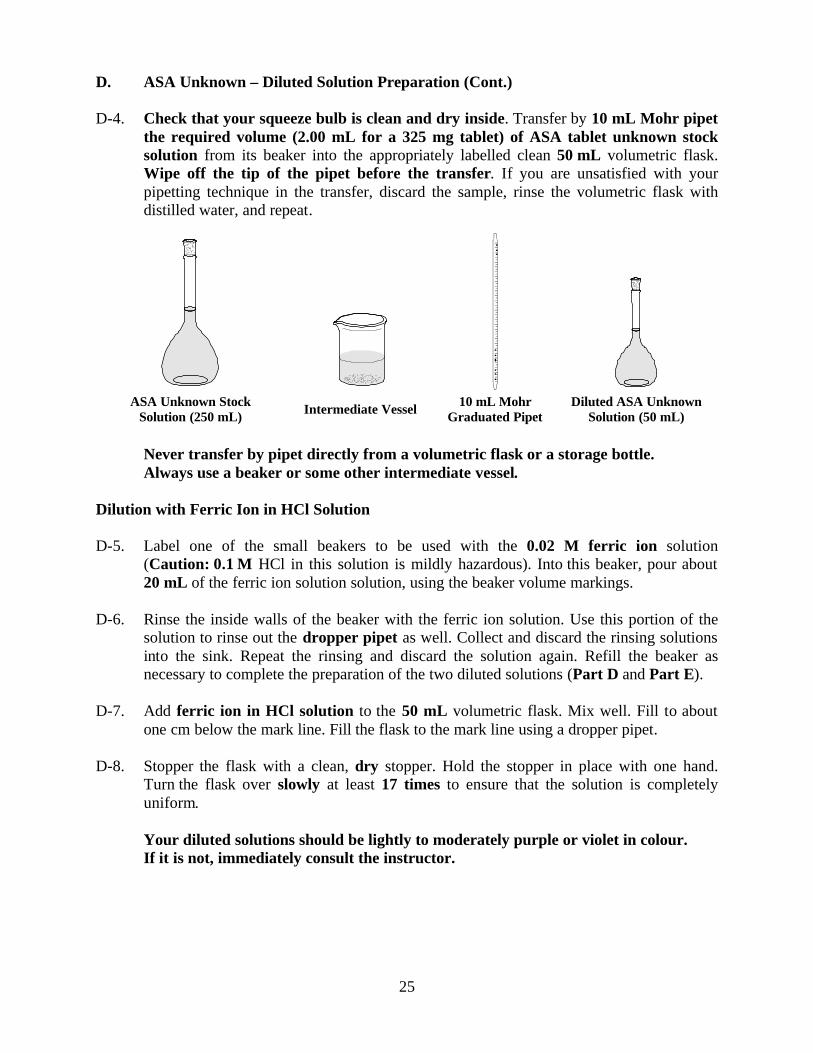
D. ASA Unknown – Diluted Solution Preparation (Cont.) D-4. Check that your squeeze bulb is clean and dry inside. Transfer by 10 mL Mohr pipet

the required volume (2.00 mL for a 325 mg tablet) of ASA tablet unknown stock solution from its beaker into the appropriately labelled clean 50 mL volumetric flask. Wipe off the tip of the pipet before the transfer. If you are unsatisfied with your pipetting technique in the transfer, discard the sample, rinse the volumetric flask with distilled water, and repeat.

ASA Unknown Stock

Solution (250 mL) Intermediate Vessel 10 mL Mohr Graduated Pipet

Diluted ASA Unknown Solution (50 mL)

Never transfer by pipet directly from a volumetric flask or a storage bottle. Always use a beaker or some other intermediate vessel. Dilution with Ferric Ion in HCl Solution D-5. Label one of the small beakers to be used with the 0.02 M ferric ion solution

(Caution: 0.1 M HCl in this solution is mildly hazardous). Into this beaker, pour about 20 mL of the ferric ion solution solution, using the beaker volume markings.

D-6. Rinse the inside walls of the beaker with the ferric ion solution. Use this portion of the

solution to rinse out the dropper pipet as well. Collect and discard the rinsing solutions into the sink. Repeat the rinsing and discard the solution again. Refill the beaker as necessary to complete the preparation of the two diluted solutions (Part D and Part E).

D-7. Add ferric ion in HCl solution to the 50 mL volumetric flask. Mix well. Fill to about

one cm below the mark line. Fill the flask to the mark line using a dropper pipet. D-8. Stopper the flask with a clean, dry stopper. Hold the stopper in place with one hand.

Turn the flask over slowly at least 17 times to ensure that the solution is completely uniform.

Your diluted solutions should be lightly to moderately purple or violet in colour. If it is not, immediately consult the instructor.

26

E. ASA Standard – Diluted Solution Preparation E-1. Transcribe the concentration of the stock standard ASA solution in mg / L units from

Table C to Table E in the DATA TABLES AND REPORT section. Pipetting the ASA Stock Standard Solution E-2. Label one clean small beaker to be used for the ASA stock standard solution. Into this

beaker, pour about 20 mL of the ASA standard solution, using the beaker volume markings.

E-3. Rinse the inside walls of the beaker with the ASA standard solution. Use this portion of

the solution to rinse out your 10 mL graduated Mohr pipet as well. Collect and discard the rinsing solutions into the sink. Repeat the rinsing and discard the solution again. On the third refill, take about 10 mL to 20 mL of the ASA standard solution into the beaker.

The instructor will assign your partnership to be one of three to five pairs working to produce a set of data for a calibration curve. You will dilute your ASA standard solution as one of the entries in the Table following. Circle your assigned number and volume here and also in Table E.

Diluted Calibration Standard No. 1 2 3 4 5

Volume of ASA Standard (mL) 1.00 2.00 3.00 4.00 5.00

Target Concentration of ASA (mg / L) 16 32 48 64 80

E-4. Check that your squeeze bulb is clean and dry inside. Transfer by 10 mL Mohr pipet your assigned volume of ASA standard solution from its beaker into the appropriately labelled clean 50 mL volumetric flask. Wipe off the tip of the pipet before the transfer. If you are unsatisfied with your pipetting technique in the transfer, discard the sample, rinse the volumetric flask with distilled water, and repeat.

ASA Standard Stock

Solution (250 mL) Intermediate Vessel 10 mL Mohr Graduated Pipet

Diluted ASA Calibration Solution (50 mL)

Never transfer by pipet directly from a volumetric flask or a storage bottle. Always use a beaker or some other intermediate vessel.


27

E. ASA Standard – Diluted Solution Preparation (Cont.) Dilution with Ferric Ion in HCl Solution E-5. Use the small beaker from Part D containing the 0.02 M ferric ion solution and the

dropper pipet (Caution: 0.1 M HCl in this solution is mildly hazardous). E-6. Add ferric ion in HCl solution to the 50 mL volumetric flask. Mix well. Fill to about

one cm below the mark line. Fill the flask to the mark line using the dropper pipet. E-7. Stopper the flask with a clean, dry stopper. Hold the stopper in place with one hand.

Turn the flask over slowly at least 17 times to ensure that the solution is completely uniform.

Your diluted solution should be lightly to moderately purple or violet in colour. If it are not, immediately consult the instructor.

28

F. Percent Transmission / Absorbance Measurements The instructor will assign your partnership and larger group to a specific spectrophotometer. There should be a large beaker near the spectrophotometer for rinse solutions and other discarded solutions. The instructor will demonstrate the preparation and use of the spectrophotometer. Each type of instrument used by the department has printed instructions for its use available in the laboratory. In general, the following steps are required: • Plug in, turn on and allow sufficient warm-up time (about 10 minutes). • Set the required wavelength (530 nm). • Adjust no transmission = 0 % transmission of light = infinite Absorbance value. • Adjust full transmission = 100 % transmission of light = zero Absorbance value.

These two adjustments are performed manually on the Spectronic 20, but are automatic on microprocessor equipped instruments.

• Clean your sample cell(s). • Reset full transmission with either distilled water or a blank solution in the cell.

F-1 You will be given a special sample test tube, or be asked to share a sample test tube with (an)other student pair(s). Clean the test tube. Rinse well with distilled water after cleaning. Be careful not to scratch the surface of the glass. You must use the same tube for all of your measurements.

Notice that the test-tube sample cell has a vertical white marker line at the top. This

marker line is used to ensure that the tube is always placed into the instrument in the same position.

F-2. When your turn on the spectrophotometer comes, check that the wavelength is set to 530

nm, but DO NOT TOUCH the wavelength setting dial if there is one. F-3. Fill your sample test tube three times with the blank solution, the 0.02 M solution of

ferric ions in 0.1 M HCl solution. Empty the blank solution out twice into a discard beaker. After the third refill, dry off the outside of the test tube carefully with the special low-lint wipes provided.

The tube needs to be only about two-thirds full; the light beam passes through the lower

part of the tube. F-4. Place the sample test tube in the sample compartment of the instrument with the white

marker line in line with the marker notch on the cell compartment. Reset full 100 % transmission (Zero Absorbance) with the blank solution in the test tube.


29

F. Percent Transmission / Absorbance Measurements (Cont.) F-5. Check and reset the 0 % transmission reading with the cell compartment empty. Be sure

that the compartment is closed to outside light for this operation. These settings interact, so you should repeat both settings at least twice more.

F-6. Empty the sample test tube into the discard beaker. Rinse the test tube with either one of

your prepared solutions twice and then fill the sample test tube a third time to be about two-thirds full. Dry the outside. Insert the test tube correctly into the instrument.

When the reading is stable, read and record the value for that solution in Table F (Trial

1) in the DATA TABLES AND REPORT section:

Spectronic 20 Other Direct Reading Instrument

Read % Transmission Scale Value to Nearest 1 %

Read Absorbance Value Displayed (All Digits)

Note: DO NOT attempt to read the Absorbance scale of the Spectronic 20 directly. The scale is not linear and is very difficult to interpret correctly. F-7. Repeat these steps for your other prepared solution. Record the value in Table F (Trial

1). F-8. Repeat the process for both solutions if time permits (Trial 2). Do not worry if the values

differ on the second reading by up to ± 2 % Transmission (or ± 0.01 Absorbance). If they differ by more than this amount, consult the instructor. F-9. Finally, repeat the process for the blank solution to check that the instrument reads 100

% Transmission (or 0.000 Absorbance) or very close to that value with the blank solution in the light beam. Do not worry if the value differs from these values by up to ± 2 % Transmission (or ± 0.01 Absorbance). If it differs by more than this amount, consult the instructor.

F-10. If you are using a Spectronic 20, you must CALCULATE the Absorbance of the two

solutions as follows:

a. Determine the mean value of % Transmission (= % T) for each solution. State the value to the nearest 1 %;

b. Calculate the value of Absorbance using this equation:

Absorbance = A = - log T = logP0

P100% T

= log

The PROCEDURE Continues on the Next Page à

30

G. Data Entry (Work with your Group) The instructor will combine your partnership with two, three, or four other partnerships as a supergroup. The data from all of the supergroup will be combined to prepare a calibration curve for the analysis which all of the pairs will be able to use for the report calculations. Each supergroup will require a recording secretary and a steering committee to assess the suitability of each point of the data set. If time permits, unsuitable data points may be re-measured. G-1 Enter the student names of each of the partnerships of the supergroup in the appropriate

cells in Table G in the DATA TABLES AND REPORT section. G-2. Enter the ASA mass and Absorbance value of the diluted solution standard for each of

the partnerships of the supergroup in the appropriate cells in Table G. G-3. Calculate and enter the values of Cconcentrated and Cdilute in each appropriate cell of Table

G. G-4. Plot the approximate positions of the values of Absorbance versus Cdilute for the data set.

Use the graph area below.

G-5. Show your Table G and the approximately plotted data values to the instructor for initialing and discussion. If your data set is to be useful, the plot should be relatively linear.

0.00

0.60

0.10

0.20

0.30

0.40

0.50

Abs

orba

nce


0 10 20 30 40 50 60 70 80 90

The REPORT Section is on the Next Page à

31

REPORT Steps R-1 to R-12 are to be carried out before leaving the laboratory.

Table B

R-1. Determine and enter the mass value of your ASA tablet unknown in Table B.

Table C

R-2. Enter your weighing data for the analytical-grade ASA in Table B.

R-3. Calculate the concentration of the ASA in the stock standard solution(Cconcentrated) in mg / L (ppm) units. State the value to 4 significant figures. Show work.

See Example 1 on page 11. Enter the value in Table C.

Table D

R-4. Circle the volume of Cconcentrated that you used in the Table.

Table E

R-5. Circle the volume of Cconcentrated that you used in the Table.

R-6. Calculate the concentration of the ASA in the diluted standard solution (Cdilute) in mg / L (ppm) units. State the value to 3 significant figures. Show work.

See Example 2 on page 11. Enter the value in Table D.

Table F

R-7. Enter the experimental values of either % Transmission or Absorbance (depending on the instrument used) measured for each of your two solutions in Table F.

R-8. Spectronic 20: Determine and enter the mean value of % Transmission for each of the two solutions in Table F, and calculate and enter the Absorbance value for each solution as instructed. Other Instruments: Determine and enter the mean value of Absorbance for each of the two solutions in Table F.

Table G

R-9. Enter the student names of the partnerships in your calibration curve supergroup in Table G.

R-10. Enter the experimental data values of ASA mass and Absorbance values of the diluted standard solutions for all partnerships in your calibration curve supergroup in Table G.

R-11. Enter the calculated values of experimental Cconcentrated and Cdilute for each standard prepared in your calibration curve group in Table G.

R-12. Verify that all of the experimental data points for the calibration set are acceptable by preparing a rough plot of the data. Re-calculate or if necessary re-measure any points which are not correctly situated, as time permits.

The REPORT Section Continues on the Next Page à

32

REPORT (Cont.)

Table G (Cont.)

The remaining steps are to be carried out after the laboratory period.

R-13. Produce a calibration curve for the analysis.

Plotting Instructions (may be done either individually or in pairs)

a. Use a software package (e.g.: Microsoft Excel®) to display an X - Y Scatter Plot of the data. Choose the no-lines option.

b. Title the plot, including your name(s) and the date, and label both axes.

c. Choose a linear least-squares best-fit trendline to the data.

d. Display the trendline on your plot and also display the equation and R2 value of the trend-line.

e. Use the cursor to select the equation box. Format as a number and choose the option five (5) places after the decimal point.

f. Attach a print-out of your completed plot to the REPORT. Analysis Calculations R-14. Use the experimental calibration curve equation to calculate the experimental ASA

concentration (Cdilute) of the diluted solution of YOUR tablet unknown in mg / L units. State the value to 1 place after the decimal point. Show work. See Example 3 on page 12. Enter the value in Analysis Calculations.

R-15. Use the dilution relationship to calculate the experimental ASA concentration

(Cconcentrated) of the stock solution of YOUR tablet unknown. For a 325 mg tablet, the dilution was from 2.00 mL volume of the concentrated solution to 50.00 mL volume of the diluted solution. State the value to the nearest 1 mg / L. Show work. See Example 4 on page 13.

Enter the value in Analysis Calculations. R-16 Use the total volume of the stock solution of the tablet unknown (0.2500 L) to calculate

the experimental total amount of ASA in YOUR tablet. State the value to the nearest 1 mg. Show work. See Example 5 on page 13.

Enter the value in Analysis Calculations. Bonus Questions (10 Points) See the Bonus Questions on page 39.

33

Name Day Start Time

DATA TABLES AND REPORT The following Tables are to be used for recording observations and measurements. Measured values are to be recorded in the heavily shaded cells IN INK. Leave this page open on your bench during the experiment period. Have it initialed by the instructor on completing each section. The completed and initialed DATA TABLES AND REPORT Section must be handed in along with any additional pages you may submit as your report. Partner’s Name: Table B: ASA Unknown – Stock Solution Preparation Description of the ASA Tablet Unknown

Brand Name and Description of the ASA Tablet Unknown

Tablet Mass (mg)

Nominal ASA Content (mg)

Table C: ASA Standard – Stock Solution Preparation ASA Target Mass: 0.20 ± 0.02 g

Weighings of Analytical-Grade Solid ASA (In Ink to 4 Places after the Decimal Point) Container + Solid (g) Container + Residue (g) Mass of ASA (g)

Instructor’s Initials: (5 points) Calculate the experimental concentration of the ASA in YOUR stock standard solution in mg / L (ppm) units. State the value to 4 significant figures. (2 points) Show work. See Example 1 on page 11. Volume of Flask Used: 250 mL = 0.2500 L

Experimental ASA Conc. of YOUR Stock Standard Solution = mg / L

The DATA TABLES AND REPORT Section Continues on the Next Page à

34

DATA TABLES AND REPORT (Cont.) Table D: ASA Unknown – Diluted Solution Preparation Circle Your Assigned Volume of Cconcentrated in the Table.

Nominal ASA Content of Tablet (mg) 81 325 650

Volume of ASA Tablet Unknown Stock Solution (mL) 8.00 2.00 1.00

Nominal Final Concentration of ASA (mg / L) 52 52 52

Table E: ASA Standard – Diluted Solution Preparation Circle Your Assigned Solution Number and Volume of Cconcentrated in the Table.

Diluted Calibration Standard No. 1 2 3 4 5

Volume of ASA Standard (mL) 1.00 2.00 3.00 4.00 5.00

Target Concentration of ASA (mg / L) 16 32 48 64 80 Concentration of the Stock Solution Standard (From Table C) = mg / L Calculate the experimental concentration of the ASA in YOUR diluted standard solution in mg / L (ppm) units. State the value to 3 significant figures. (2 points) Show work. See Example 2 on page 11. Volume of Flask Used: 50.00 mL Experimental ASA Concentration of YOUR Diluted Standard Solution = mg / L


35

Name Day Start Time

DATA TABLES AND REPORT (Cont.) Table F: Percent Transmission / Absorbance Measurements If Using the Spectronic 20

Percent Transmission Values (In Ink) to the Nearest 1 % Trial 1 Trial 2 Mean % T

% Transmission Value of Diluted Standard

% Transmission Value of Diluted Tablet Unknown

Calculated Absorbance Values to 3 Places

Absorbance = A = - log T = log

P0

P100% T

= log

Example: Mean % T = 35 %

10035

Absorbance = log = 0.456

Show a Sample Calculation If Using a Direct Reading Instrument

Absorbance Values (In Ink) to 3 Figures Trial 1 Trial 2 Mean A

Absorbance Value of Diluted Standard

Absorbance Value of Diluted Tablet Unknown

Instructor’s Initials on Completion: (10 points)


Mean % T Calculated Absorbance

Diluted Standard

Diluted Tablet Unknown

36

DATA TABLES AND REPORT (Cont.) Table G: Data Entry

Partnership Names

Standard 1 and

Standard 2 and

Standard 3 and

Standard 4 and

Standard 5 and

Calculated Concentrations and Absorbance Values of the ASA Solution Standards Standard 1 Standard 2 Standard 3 Standard 4 Standard 5

ASA Mass (g)

Calculated ASA Cconcentrated

(mg / L)

ASA Target Cdilute (mg / L) 16 32 48 64 80

Dilution of ? mL to 50.00 mL 1.00 mL 2.00 mL 3.00 mL 4.00 mL 5.00 mL

Calculated ASA Cdilute

(mg / L)

Mean Experimental Absorbance

Instructor’s Initials on Completion: (10 points)


37

Name Day Start Time

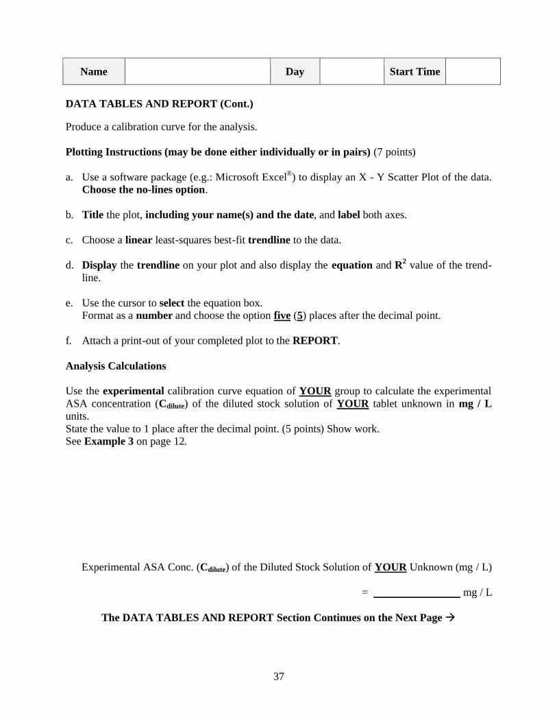
DATA TABLES AND REPORT (Cont.) Produce a calibration curve for the analysis. Plotting Instructions (may be done either individually or in pairs) (7 points) a. Use a software package (e.g.: Microsoft Excel®) to display an X - Y Scatter Plot of the data.

Choose the no-lines option. b. Title the plot, including your name(s) and the date, and label both axes. c. Choose a linear least-squares best-fit trendline to the data. d. Display the trendline on your plot and also display the equation and R2 value of the trend-

line. e. Use the cursor to select the equation box.

Format as a number and choose the option five (5) places after the decimal point. f. Attach a print-out of your completed plot to the REPORT. Analysis Calculations Use the experimental calibration curve equation of YOUR group to calculate the experimental ASA concentration (Cdilute) of the diluted stock solution of YOUR tablet unknown in mg / L units. State the value to 1 place after the decimal point. (5 points) Show work. See Example 3 on page 12.

Experimental ASA Conc. (Cdilute) of the Diluted Stock Solution of YOUR Unknown (mg / L)

= mg / L


38

DATA TABLES AND REPORT (Cont.) Analysis Calculations (Cont.) Use the dilution relationship to calculate the experimental ASA concentration (Cconcentrated) of the stock solution of YOUR tablet unknown. For a 325 mg tablet, the dilution was from 2.00 mL volume of the concentrated solution to 50.00 mL volume of the diluted solution. State the value to the nearest 1 mg / L. (2 points) Show work. See Example 4 on page 13.

Experimental ASA Conc. (Cconcentrated) of the Stock Solution of YOUR Unknown (mg / L)

= mg / L Use the total volume of the stock solution of the tablet unknown (0.2500 L) to calculate the experimental total amount of ASA in YOUR tablet. State the value to the nearest 1 mg. (2 points) Show work. See Example 5 on page 13.

Experimental Total ASA Content of YOUR Tablet Unknown (mg) = mg

The Bonus Questions and the Mark Sheet are on the Next Two Pages à

39

Name Day Start Time

DATA TABLES AND REPORT (Cont.) Bonus Questions (10 Points) Attach a separate page of calculations. 1. Calculate the ASA concentration (Cdilute) in YOUR diluted tablet unknown solution by the

method of proportion. Use only your own data for YOUR diluted standard and YOUR diluted tablet unknown solution. State the value to the nearest 0.1 mg / L. (6 points) Show work. See Example 6 on page 14.

2. Use the dilution relationship to calculate the ASA concentration (Cconcentrated) of the stock

solution of YOUR tablet unknown using the value of Cdilute calculated as the answer to Bonus Question 1. For a 325 mg tablet, the dilution was from 2.00 mL volume of the concentrated solution to 50.00 mL volume of the diluted solution. State the value to the nearest 1 mg / L. (2 points) Show work. See Example 4 on page 13.

3. Use the total volume of the stock solution of the tablet unknown (0.2500 L) to calculate the

total amount of ASA in YOUR tablet unknown using the value of Cconcentrated calculated as the answer to Bonus Question 2. State the value to the nearest 1 mg. (2 points) Show work. See Example 5 on page 13.

The Mark Sheet is on the Next Page à

40

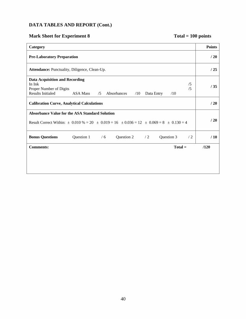
DATA TABLES AND REPORT (Cont.) Mark Sheet for Experiment 8 Total = 100 points Category Points

Pre-Laboratory Preparation / 20

Attendance: Punctuality, Diligence, Clean-Up. / 25

Data Acquisition and Recording In Ink /5 Proper Number of Digits /5 Results Initialed ASA Mass /5 Absorbances /10 Data Entry /10

/ 35

Calibration Curve, Analytical Calculations / 20

Absorbance Value for the ASA Standard Solution Result Correct Within: ± 0.010 % = 20 ± 0.019 = 16 ± 0.036 = 12 ± 0.069 = 8 ± 0.130 = 4

/ 20

Bonus Questions Question 1 / 6 Question 2 / 2 Question 3 / 2 / 10

Comments: Total = /120

Documents

Spectrometry: Quantitative Determination of ASA by ... · PDF fileThis Experiment is a 3 hour Analytical Chemistry ... The beneficial properties of salicylic acid ... (Ethanoic Acid)