Spectral Modelling for Transformation and Separation of

Spectral Modelling for

Transformation and Separation of

Audio Signals

Thomas Arvanitidis

MSc by research

University of York

Electronics

December 2014

Abstract

The Short-Time Fourier Transform is still one of the most promi-

nent time-frequency analysis techniques in many fields, due to its

intuitive nature and computationally-optimised basis functions. Nev-

ertheless, it is far from being the ultimate solution as it is plagued

with a variety of assumptions and user-specific design choices, which

result in a number of compromises. Numerous attempts have been

made to circumvent its inevitable internal deficiencies, which include

fixed time-frequency resolutions, static sample points, and highly bi-

ased outputs. However, its most important assumption, stationarity,

is yet to be dealt with effectively. A new concept is proposed, which

attempts to improve the credibility of the STFT results by allowing a

certain degree of deviation from stationarity to be incorporated into

the analysis. This novel approach utilises an ensemble of estimates

instead of a single estimation in order to investigate the short-time

phase behaviour of every frequency bin. The outcome is the defi-

nition of a quality measure, phase stability, that discriminates the

“structured” from the “artefact” frequency components. This quality

measure is then used in the framework of source separation as a sin-

gle application example where it is possible to investigate its potential

on the performance of the algorithm. Specifically, it was used in the

spectral peak picking step of a numerical model-based source separa-

tion algorithm. It was found that the phase stability quality measure

acts as an effective data reduction tool, which qualifies it as a more

appropriate thresholding technique than the conventional methods.

Based on this example, it is anticipated that this new method has

great potential. Its ability to discriminate between “structured” and

“noise” or edge effect/“artefacts” qualifies it as a promising new tool

that can be added in the arsenal of the STFT modifications and used

in the development of a hybrid super-STFT.

ii

Contents

Abstract ii

Contents iii

List of Figures vi

List of Tables x

Acknowledgements xi

Author’s Declarations xii

1 Introduction 1

1.1 Report Overview . . . . . . . . . . . . . . . . . . . . . . . . . . . 3

2 Background 4

2.1 Note Structure: ADSR, Partials and Harmonics . . . . . . . . . . 4

2.2 Sinusoidal Model . . . . . . . . . . . . . . . . . . . . . . . . . . . 7

2.3 Spectral Analysis . . . . . . . . . . . . . . . . . . . . . . . . . . . 8

2.3.1 Discrete Fourier Transform . . . . . . . . . . . . . . . . . . 10

2.3.1.1 Windowing . . . . . . . . . . . . . . . . . . . . . 16

2.3.2 Short-Time Fourier Transform . . . . . . . . . . . . . . . . 17

2.3.3 Discussion . . . . . . . . . . . . . . . . . . . . . . . . . . . 20

2.3.3.1 DFT versus FFT . . . . . . . . . . . . . . . . . . 20

2.3.3.2 Single-estimate versus Multiple-estimate Averaged

Spectrograms . . . . . . . . . . . . . . . . . . . . 20

iii

2.3.3.3 STFT parameter setting . . . . . . . . . . . . . . 20

2.3.3.4 Practical implementation of the STFT . . . . . . 22

2.3.3.5 ISTFT . . . . . . . . . . . . . . . . . . . . . . . . 23

2.3.4 STFT Modifications . . . . . . . . . . . . . . . . . . . . . 24

2.3.4.1 Multiresolution . . . . . . . . . . . . . . . . . . . 25

2.3.4.2 Adaptive STFT . . . . . . . . . . . . . . . . . . . 26

2.3.4.3 Frequency Reassignment . . . . . . . . . . . . . . 28

2.3.4.4 Multitapers . . . . . . . . . . . . . . . . . . . . . 28

2.3.5 Summary . . . . . . . . . . . . . . . . . . . . . . . . . . . 29

3 Phase Stability Quality Measure 31

3.1 Motivation: PASS with EASE . . . . . . . . . . . . . . . . . . . . 32

3.2 Research Hypothesis, Aims and Objectives . . . . . . . . . . . . . 32

3.3 Principles . . . . . . . . . . . . . . . . . . . . . . . . . . . . . . . 33

3.3.1 Stationary Signals . . . . . . . . . . . . . . . . . . . . . . . 34

3.3.2 Non-Stationary Signals . . . . . . . . . . . . . . . . . . . . 41

3.4 Examples . . . . . . . . . . . . . . . . . . . . . . . . . . . . . . . 49

3.5 Summary . . . . . . . . . . . . . . . . . . . . . . . . . . . . . . . 58

4 PhiStab Function 59

4.1 STFT Modification: Construction of the ensemble of estimates . . 59

4.2 PhiStab Function . . . . . . . . . . . . . . . . . . . . . . . . . . . 62

4.3 Testing . . . . . . . . . . . . . . . . . . . . . . . . . . . . . . . . . 64

4.3.1 STFT Testing . . . . . . . . . . . . . . . . . . . . . . . . . 64

4.3.2 PhiStab Testing . . . . . . . . . . . . . . . . . . . . . . . . 65

4.4 Summary . . . . . . . . . . . . . . . . . . . . . . . . . . . . . . . 66

5 Phase Stability with Source Separation 68

5.1 Source Separation: Definition and history of the problem . . . . . 68

5.2 Motivation, Aims and Objectives . . . . . . . . . . . . . . . . . . 70

5.3 The Algorithm . . . . . . . . . . . . . . . . . . . . . . . . . . . . 74

5.3.1 Specification . . . . . . . . . . . . . . . . . . . . . . . . . . 74

5.3.2 Design . . . . . . . . . . . . . . . . . . . . . . . . . . . . . 75

5.3.2.1 Declaration of the parameters . . . . . . . . . . . 76

iv

5.3.2.2 Import of the subject signals . . . . . . . . . . . 76

5.3.2.3 Analysis . . . . . . . . . . . . . . . . . . . . . . . 76

5.3.2.4 Voting system . . . . . . . . . . . . . . . . . . . . 77

5.3.2.5 Separation and resynthesis . . . . . . . . . . . . . 82

5.4 Result Review . . . . . . . . . . . . . . . . . . . . . . . . . . . . . 82

6 Conclusions 86

7 Further Work 88

7.1 Phase Stability . . . . . . . . . . . . . . . . . . . . . . . . . . . . 88

7.2 Source Separation . . . . . . . . . . . . . . . . . . . . . . . . . . . 90

Appendix A: Initial phase angles obtained from the analysis of the

cosine in chapter 3 93

Appendix B: Initial phase angles obtained from the analysis of the

cosine with vibrato in chapter 3 94

Appendix C: Initial phase angles obtained from the analysis of the

cosine with glissando in chapter 3 95

Appendix D: Application of artificial vibrato on the violin sample

in Cubase 7.5 96

Appendix E: Application of artificial glissando on the violin sample

in Cubase 7.5 97

Appendix F: The stft function 98

Appendix G: The phistab function 102

Nomenclature 106

References 109

v

List of Figures

2.1 ADSR model . . . . . . . . . . . . . . . . . . . . . . . . . . . . . 5

2.2 The spectral structure of a guitar pluck (frame length = 8192,

overlap = 98.4375% , zpf = 2) (The white spots are artefacts due

to screen resolution) . . . . . . . . . . . . . . . . . . . . . . . . . 6

2.3 The relationship between the temporal and spectral representa-

tions of a rectangular function [10]. . . . . . . . . . . . . . . . . . 9

2.4 Arbitrary selection of a portion of an infinite signal and its periodic

finite form as considered by DFT . . . . . . . . . . . . . . . . . . 14

2.5 The rectangular window and its spectrum . . . . . . . . . . . . . 15

2.6 Illustration of the case where the amplitude spectral components

of a signal coincide with the nulls of the sidebands of the ampli-

tude spectrum of the rectangular window function. The amplitude

spectrum of the window function has been delineated with the help

of zero padding . . . . . . . . . . . . . . . . . . . . . . . . . . . . 15

2.7 Spectrogram of a linear chirp sampled at 1024 Hz and total length

1024 samples that starts at DC at sample 1 and crosses 0.5859 at

sample 512. STFT parameters: frame length = 256, overlap =

75%, zpf = 0, window function = Hamming . . . . . . . . . . . . 18

2.8 Various time-frequency resolutions . . . . . . . . . . . . . . . . . . 21

2.9 Illustration of the obtainment of a spectrogram with the practical

implementation of STFT. The first quarter of the signal is depicted

in a), which is analysed with a Hamming window function (due

to spectrogram function in MATLAB). N = 12288, L = 1024,

H = 1024, zpf = 0 . . . . . . . . . . . . . . . . . . . . . . . . . . 23

vi

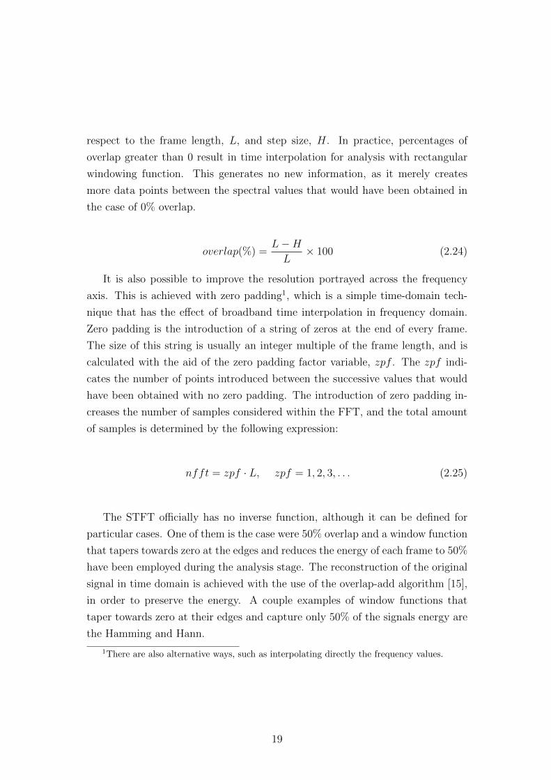
2.10 Grid representation of a multiresolution approach . . . . . . . . . 25

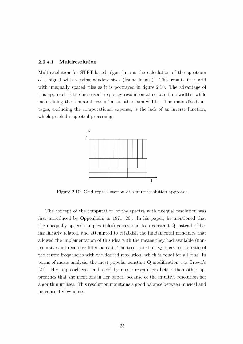
2.11 Grid representation of an ASTFT approach . . . . . . . . . . . . 26

2.12 ASTFT: Illustrating the use of variable block size with respect to

content, which results in smaller amounts of time smearing [22] . . 27

3.1 (a) Representation of an idealised cosine (N = 128, T = 16, ϕ(0) =

0). (b) The wrapped phase angle values of the signal depicted in a)

as calculated during its generation. (c) The logarithmic amplitude

spectrum of the signal depicted in a). A single peak is depicted as

expected due to the lack of discontinuities, with all the rest of the

sampled frequency components being virtually zero . . . . . . . . 35

3.2 Hypothetical scenario of ensemble of closely-related estimates ap-

plied to the signal of 3.1-a) . . . . . . . . . . . . . . . . . . . . . . 36

3.3 The periodic version of the wrapped phase angle values of the

framed signals depicted in figure 3.2, as considered by FFT . . . . 37

3.4 The logarithmic amplitude spectra of the framed signals of figure

3.2 . . . . . . . . . . . . . . . . . . . . . . . . . . . . . . . . . . . 37

3.5 Initial phase angle value variation for each estimate, as obtained

from FFT, for bins 4 and 18 . . . . . . . . . . . . . . . . . . . . . 39

3.6 Initial phase angle value variation for each estimate as obtained

from FFT against the modelled phase angle values of an idealistic

frequency component for two representative bins . . . . . . . . . . 40

3.7 (a) Deviation of the phase values calculated by FFT from the mod-

elled phase values of an idealistic frequency component for bin 4.

(b) Deviation of the phase values calculated by FFT from the mod-

elled phase values of an idealistic frequency component for bin 18.

(c) Phase Stability: The sum of the least squares of the deviation

for each bin . . . . . . . . . . . . . . . . . . . . . . . . . . . . . . 40

3.8 (a) Representation of the idealised cosine with vibrato. (b) The

wrapped phase angle values of the signal depicted in a) as calcu-

lated during its generation. (c) The logarithmic amplitude spec-

trum of the signal depicted in a) . . . . . . . . . . . . . . . . . . . 43

vii

3.9 (a) Representation of the idealised chirp. (b) The wrapped phase

angle values of the signal depicted in a) as calculated during its

generation. (c) The logarithmic amplitude spectrum of the signal

depicted in a) . . . . . . . . . . . . . . . . . . . . . . . . . . . . . 44

3.10 The unwrapped phase angle values of the cosine with vibrato de-

picted in fig. 3.8-a) as calculated during the signal’s generation. . 45

3.11 The unwrapped phase angle values of the chirp depicted in fig.

3.9-a) as calculated during the signal’s generation . . . . . . . . . 45

3.12 Phase coefficients as obtained from FFT for the cosine with vi-

brato against the modelled phase values of an idealistic frequency

component . . . . . . . . . . . . . . . . . . . . . . . . . . . . . . . 47

3.13 (a) Deviation of the actual phase values calculated by FFT from

the modelled phase values of an idealistic frequency component

with vibrato for bin 4. (b) Deviation of the actual phase values

calculated by FFT from the modelled phase values of an idealistic

frequency component with vibrato for bin 18. (c) Phase Stability:

The sum of the least squares of the deviation for each bin . . . . . 47

3.14 Phase coefficients as obtained from FFT for the chirp against the

modelled phase values of an idealistic frequency component . . . . 48

3.15 (a) Deviation of the actual phase values calculated by FFT from

the modelled phase values of an idealistic frequency sweep for bin

8. (b) Deviation of the actual phase values calculated by FFT

from the modelled phase values of an idealistic frequency sweep

for bin 18. (c) Phase Stability: The sum of the least squares of the

deviation for each bin. . . . . . . . . . . . . . . . . . . . . . . . . 48

3.16 Analysed data of the 2nd frame of the synthetic signal with 4 sta-

tionary components (a) Phase stability. (b) Inverse phase stability.

(c) Amplitude spectra . . . . . . . . . . . . . . . . . . . . . . . . 51

3.17 Analysed data of the 2nd frame of the synthetic signal with 3 near-

stationary components (signal with vibrato). (a) Phase stability.

(b) Inverse phase stability. (c) Amplitude spectra . . . . . . . . . 52

viii

3.18 Analysed data of the 2nd frame of the synthetic signal with 3 non-

stationary components (signal with glissando). (a) Phase stability.

(b) Inverse phase stability. (c) Amplitude spectra . . . . . . . . . 53

3.19 Analysed data of the 2nd frame of the signal of an A4 violin note.

(a) Phase stability. (b) Inverse phase stability. (c) Amplitude spectra 54

3.20 Analysed data of the 2nd frame of the signal of an A4 violin note

with vibrato. (a) Phase stability. (b) Inverse phase stability. (c)

Amplitude spectra . . . . . . . . . . . . . . . . . . . . . . . . . . 56

3.21 Analysed data of the 2nd frame of the signal of an A4 violin note

with glissando. (a) Phase stability. (b) Inverse phase stability. (c)

Amplitude spectra . . . . . . . . . . . . . . . . . . . . . . . . . . 57

5.1 Generic structure of an idealised model-based source separation

algorithm applied to a single-track audio signal . . . . . . . . . . 69

5.2 An example of a thresholded spectrum from Benson’s work [53] (a)

Original spectrum of mixture of cello and flute notes of different

pitches. (b) Processed (data-reduced) spectrum of a) with the aid

of a threshold. The units of the x and y axis are seconds and hertz,

respectively . . . . . . . . . . . . . . . . . . . . . . . . . . . . . . 71

5.3 Example of various thresholding functions. Spectrum of mixture

of violin and flute notes with a static threshold (Flute f0 = 293 Hz,

Violin f0 = 510 Hz) (b) Every’s adaptive thresholding technique

on the spectrum of an oboe note (f0 = 293 Hz) [54] . . . . . . . . 73

5.4 Analysis routine 1 of the source separation algorithm: Conven-

tional STFT Mode . . . . . . . . . . . . . . . . . . . . . . . . . . 78

5.5 Analysis routine 2 of the source separation algorithm: Phase Sta-

bility Enhanced Spectrum Mode . . . . . . . . . . . . . . . . . . . 79

5.6 Example of a harmonic model with 32 partials . . . . . . . . . . . 81

5.7 Analysis of a mixture of violin and flute notes. (a) Conventional

amplitude spectrum (b) Phase Stability Enhanced Spectrum (PSES)

with threshold value 0.009 (c) Phase Stability Enhanced Spectrum

(PSES) with threshold value 0.09 . . . . . . . . . . . . . . . . . . 84

ix

List of Tables

2.1 Specification of a few popular window functions . . . . . . . . . . 17

2.2 Lowest accurately estimated frequency with respect to different

frame lengths (based on [19]) . . . . . . . . . . . . . . . . . . . . 22

3.1 User-specific design choices of STFT and their implications . . . . 32

3.2 Initial phase for every frame estimate for bin 4 and 18 . . . . . . . 38

3.3 Initial phase angle values for bin 4 and 18 for the cosine with vibrato 46

3.4 Initial phase angle values for bin 8 and 18 for the chirp . . . . . . 46

3.5 Phase stability analysis parameters for the analysis of the signals . 50

3.6 Point values marked in graph b) and c) of figure 3.19. . . . . . . . 54

3.7 Point values marked in graph b) and c) of figure 3.21 . . . . . . . 57

4.1 Pseudo code of the conventional STFT algorithm . . . . . . . . . 61

4.2 Pseudo code of the modified STFT algorithm that implements the

ensemble of estimates approach . . . . . . . . . . . . . . . . . . . 62

4.3 Pseudo code of the function that calculates the phase stability

quality measure . . . . . . . . . . . . . . . . . . . . . . . . . . . . 63

4.4 List of arguments, along with their type and description, for the

stft function . . . . . . . . . . . . . . . . . . . . . . . . . . . . . . 65

4.5 List of arguments, along with their type and description, for the

phistab function . . . . . . . . . . . . . . . . . . . . . . . . . . . . 66

5.1 Analysis parameters for both conventional and phase stability en-

hanced modes . . . . . . . . . . . . . . . . . . . . . . . . . . . . . 83

x

Acknowledgements

I would like to express my deepest appreciation to all those who provided me the

possibility to complete this report. A special gratitude I give to my supervisor,

John, whose contribution in stimulating suggestions and encouragement helped

me to coordinate my project.

xi

Author’s Declarations

I declare that this thesis is a presentation of original work and I am the sole

author. This work has not previously been presented for an award at this, or any

other, University. All sources are acknowledged as References.

xii

Chapter 1

Introduction

The inspection of the frequency content of a signal is often required in order,

for instance, to learn more about the frequency behaviour of the system from

which the signal has come. Furthermore, the direct application of processing

routines, such as filtering, on the frequency content of a signal may be preferred

due to greater intuitiveness. It is, therefore, necessary to be able to transform the

signal from its temporal representation into a spectral representation to enable

such opportunities. This is achieved with the utilisation of spectral analysis

techniques.

There are several techniques that accomplish the transformation of a signal

from the time to frequency domain, and vice versa, with one of the most promi-

nent being the family of Fourier approaches. Fourier techniques continue to be

some of the dominant spectral analysis tools due to their intuitive nature and

computationally-optimised basis functions. They, in particular in the form of the

Short-Time Fourier Transform (STFT), can be found implemented in fields as

diverse as physics [1], astronomy [2], chemistry [3], medical engineering [4] and

geophysics [5].

Fourier approaches are plagued, however, with numerous assumptions and

user-specific design choices, which result in a variety of compromises. One of

the most important assumptions is stationarity. This may be disadvantageous

because the frequency content of the signal may vary with respect to time, which

may result in misleading data. In terms of user-specific design choices, the choice

to focus on the amplitude information of the analysed data and ignore the phase

1

information results in incomplete analysis.

Over the years, researchers have developed adaptations of the STFT in order

to compensate for its deficiencies but the assumption of stationarity is yet to

be tackled effectively. Moreover, the majority of the approaches solely focus

on the improvement of the credibility of the amplitude information without the

consideration of the phase information. It is, then, proposed in this project a

novel approach that involves the inspection of the short-time phase behaviour of

the signal with the construction of an ensemble of estimates, which allows the

incorporation of a certain degree of deviation from stationarity into the analysis

process. This method is based on the hypothesis that the phase behaviour of

the sampled frequency components that arise due to partials manifest structured

patterns, whereas the phase behaviour of the sampled frequency components

that arise due to statistical noise or Fourier related artefacts exhibit randomness.

This is then exploited in order to produce a quality measure that aids in the

discrimination of the “structured” from the “artefact” frequency components.

The attainment of a series of objectives is required for the implementation

of this novel concept, which include the thorough investigation of the phase be-

haviour of a set of elementary synthetic example signals as calculated at their

generation and obtained from the STFT in order to gain an insight and effi-

ciently exploit it in the analysis stage, and the development of the processing

tool that calculates the quality measure. The potential of this quality measure is

then investigated with its incorporation in the framework of source separation as

an application example.

The work conducted in this project is documented in the following chapters,

starting with the essential theoretical background of the concepts utilised. The

main research on the phase behaviour of simple synthetic signals, the calculation

of the quality measure, the documentation of the modifications applied on the

STFT algorithm in order to construct the ensemble of estimates, and the function

that calculates the phase stability are then detailed. Finally, the incorporation of

the phase stability quality measure in a numerical model-based source separation

algorithm is explained.

2

1.1 Report Overview

Chapter 1 - An introduction to this project is provided in order to inform the

reader about the topics on which this thesis elaborates and the scope of the re-

search.

Chapter 2 - This chapter provides the historical and theoretical background of

the main concepts and tools that are utilised in this project.

Chapter 3 - The main research conducted in this project is documented in this

chapter. An overview of the assumptions and user-specific design choices of the

STFT linked to their compromises is provided, followed by the motivation for

this project, the investigation of the phase behaviour of a set of elementary syn-

thetic signals with regards to the proposed method, and a few examples of the

behaviour of the phase stability of both synthetic and real signals.

Chapter 4 - The documentation of the two main functions developed for the

calculation of the phase stability is included in this chapter.

Chapter 5 - The work carried out on source separation is described in this chapter.

It initially provides a brief historical and theoretical background on source sepa-

ration with a focus on the type of the source separation algorithm implemented

in this project, the motivation and reasoning for the consideration of source sep-

aration as an application example, the documentation of the algorithm, and the

result analysis.

Chapter 6 - The findings and conclusions drawn for this projects are summarised

in this chapter.

Chapter 7 - An agenda is compiled with a set of objectives to be attained for

further validation and performance improvement of the proposed method.

3

Chapter 2

Background

This chapter provides the theoretical and historical background of the topics on

which this project elaborates. More specifically, it reviews the background of

the simplest structure found in a signal as considered by the source separation

algorithm in chapter 5, describes the model that was utilised for the generation

of the test signals that were used for the establishment of the principles of the

phase stability quality measure in chapter 3, and provides a thorough review of

the main spectral analysis method on which this research is conducted.

2.1 Note Structure: ADSR, Partials and Har-

monics

The ADSR (acronym for Attack-Sustain-Decay-Release) is a temporal represen-

tation of the different stages that a note goes through, starting from the moment

it is played until it ceases to exist. This model can be used for both real and

synthetic sounds1. Each stage manifests different properties, and varies for every

instrument. The following figure (fig. 2.1) portrays the generic structure of a note

as described by the ADSR model. It is not clear when it was first introduced but

according to Pinch [6] this model was suggested to Robert Moog from Vladimir

Ussachevsky, and first appeared in this form on the ARP Odyssey synthesiser in

1972 [7]. Moorer also uses this model for the production of digital signals in his

paper on computer music [8] but refers to it as ‘control function’. The following

1Often used in the amplification stage of synthesisers.

4

paragraphs detail the characteristics of each phase of the ADSR model.

Figure 2.1: ADSR model

The attack phase, which indicates the beginning of a note, is the first stage.

It is the phase where energy is first injected to the instrument. It may occur

in various ways depending on the type of instrument, i.e. pluck for stringed

instruments, blow for wind instruments, struck for percussive instruments. The

length of this phase is usually very short. It is also complex, in the sense that it is

not easily emulated with simple models, i.e. sinusoidal (detailed in section 2.2).

In terms of spectral behaviour, this stage is chaotic and wideband because the

energy has just been introduced to the vibrating medium and has not completely

spread across it in order to form standing waves or modes, depending on the type

of instrument.

Following the attack comes the decay phase, which is also relatively short in

time. This stage is the transition between the chaotic behaviour of the instrument

due to the travelling waves and the settling of the energy with the formation

of standing waves. It is usually very subtle in real instruments, but can have

dramatic effects in sounds generated by synthesisers.

The sustain is the next phase. It is usually the longest phase of a note. At this

stage the standing waves or modes have been formed and the chaotic wideband

spectral behaviour has become narrower and better defined. This stage may also

be prolonged due to the continuous input of energy, i.e. blowing a flute steadily.

The harmonic part (described in the following paragraphs) of the sound is more

dominant at this stage.

5

The last stage is the release, which indicates the beginning of the end of a note.

This is the stage where the amplitude of the note gradually tapers to zero. It may

be long as well as short, depending on the physical attributes of the instrument,

i.e. the sound of a bell and the sound of a snare.

All aforementioned stages differ for every instrument but also with respect

to performance styles. A hard struck on the tom of a drum kit may result in a

significantly long release, whereas a gentle strike might result in short release.

The spectral structure of a note describes its content in terms of partials, P

[9]. Partials are the frequency components that constitute the sound. They are

usually better defined in the sustain part of a note, where the standing waves and

modes have been formed. The following figure illustrates the spectral structure

of a guitar pluck.

Figure 2.2: The spectral structure of a guitar pluck (frame length = 8192, overlap= 98.4375% , zpf = 2) (The white spots are artefacts due to screen resolution)

Harmonics are the partials of a sound that are an integer multiple of the

fundamental partial [9]. A pleasant sound usually manifests a high degree of

harmonicity, i.e. a violin note. It is important to stress that the first harmonic

partial of a sound is the fundamental frequency. The expression that describes

6

the dth harmonic is:

fd = d · f0, d = 1, 2, . . . (2.1)

In the previous example (figure 2.2), there are 18 harmonics present in total.

Also it is worth noting the difference in length between the lower and higher

harmonics. High harmonics tend to decay faster than the lower harmonics for

real instruments.

2.2 Sinusoidal Model

The typical sinusoidal model is defined as the summation of numerous sinusoidal

components with different frequencies [8]. Each sinusoidal function is considered

to be a partial, p, with static amplitude, A, angular frequency, ω, and initial

phase angle, φ(0). This model is described by the following equation.

x(t) ,P∑p=1

Ap sin(ωpt+ φp(0)), t ∈ R (2.2)

A more realistic and complex version of this model, which is also the one that

is used in this project, considers the argument of the sinusoidal function as its

phase, and allows the amplitude and angular frequency of each component to

vary with respect to time.

x(t) ,P∑p=1

Ap(t) sin(ϕp(t)), t ∈ R (2.3)

where the following expressions hold:

ωp(t) =dϕpdt

(t) = 2πfp(t), p = 1, 2, . . . , P (2.4)

7

ϕp(t) = 2π

∫ t

0

fp(u)du+ φp(0), p = 1, 2, . . . , P (2.5)

The functions ωp(t) and fp(t) represent the angular frequency of the pth partial

in radians and hertz respectively, and the scalar φp(0) is the initial phase angle

of the pth partial.

The sinusoidal model allows the generation of sounds by manipulating their

spectral characteristics. It is very simple and achieves the faithful reproduction

of the sounds generated by many real instruments, such as flute and violin. More-

over, it achieves the generation of interesting synthetic soundscapes. The complex

version of the sinusoidal model (eq. 2.3) is preferred here because it allows the

production of non-stationary sound examples.

2.3 Spectral Analysis

Spectral analysis achieves the expression of the contents of a signal in terms

of amplitude and phase variations with respect to frequency. The observation

of the signal’s contents from this point of view is often beneficial because it

unveils patterns about its frequency contents that are not visible in the temporal

form. Also, certain processing routines become more intuitive and simpler, such

as filtering, since it provides direct access to the frequency components of the

signal.

There are numerous analysis techniques that achieve the transformation of

a signal into the frequency domain. However, there is not a single one that is

appropriate for all signals. This project concentrates on the Short-Time Fourier

Transform (STFT), and implicitly Discrete Fourier Transform (DFT), because of

its wide use in signal processing, and particularly on music signals.

The Discrete Fourier Transform transfers the whole signal from time to fre-

quency domain by describing it in terms of its basis. This basis is a set of

narrowband spectral components (sinusoids) that are described in terms of fre-

quency. When the transformation is finished, the entire signal is averaged into a

8

single spectrum, which describes the amount and initial phase of each sinusoid

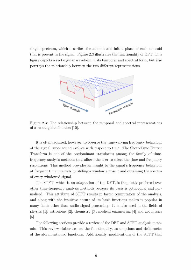
that is present in the signal. Figure 2.3 illustrates the functionality of DFT. This

figure depicts a rectangular waveform in its temporal and spectral form, but also

portrays the relationship between the two different representations.

Figure 2.3: The relationship between the temporal and spectral representationsof a rectangular function [10].

It is often required, however, to observe the time-varying frequency behaviour

of the signal, since sound evolves with respect to time. The Short-Time Fourier

Transform is one of the predominant transforms among the family of time-

frequency analysis methods that allows the user to select the time and frequency

resolutions. This method provides an insight to the signal’s frequency behaviour

at frequent time intervals by sliding a window across it and obtaining the spectra

of every windowed signal.

The STFT, which is an adaptation of the DFT, is frequently preferred over

other time-frequency analysis methods because its basis is orthogonal and nor-

malised. This attribute of STFT results in faster computation of the analysis,

and along with the intuitive nature of its basis functions makes it popular in

many fields other than audio signal processing. It is also used in the fields of

physics [1], astronomy [2], chemistry [3], medical engineering [4] and geophysics

[5].

The following sections provide a review of the DFT and STFT analysis meth-

ods. This review elaborates on the functionality, assumptions and deficiencies

of the aforementioned functions. Additionally, modifications of the STFT that

9

attempt to overcome particular limitations are examined. Finally, a list of com-

ments is consolidated regarding to the aspects that were not considered.

2.3.1 Discrete Fourier Transform

The Discrete Fourier Transform is the digital implementation of the Fourier series

[11]. The difference between the DFT and the rest of the Fourier transforms is

that its input and output signals are both discrete and finite. It also assumes

that the signal under analysis is periodic. The DFT transforms the signal, x[n]

of N samples, to the discrete frequency domain by sequentially projecting it on

a set of sinusoid functions, sk[n] of period N samples, which constitute the basis

of the Fourier dimension. The following material and equations can be found in

[11], unless otherwise stated. Different notation was used where necessary for

consistency purposes.

sk[n] , cos(ϕk[n]) + j sin(ϕk[n]) ≡ ejϕk[n], n = 0, 1, . . . , N − 1 (2.6)

X[k] ,N−1∑n=0

x[n]e−jϕk[n], k = 0, 1, . . . , N − 1 (2.7)

where

ϕk[n] = 2πfkn+ φk[0], n = 0, 1, . . . , N − 1 (2.8)

fk =k

N, k = 0, 1, . . . , N − 1 (2.9)

An alternative notation of the DFT uses the inner product operator. This

is more compact and intuitive because the projection of the signal, x[n], on the

Fourier basis, sk[n], is more apparent.

10

X[k] , 〈x[n], sk[n]〉 (2.10)

The transformation of the signal x[n] of N samples results in N complex

frequency coefficients, X[k]. These coefficients express the degree of correlation

of the signal, x[n], with the Fourier basis, sk[n]. In practice, they describe the

amplitude, A[k], and initial phase angle, φ[k], of each sinusoid. This set of com-

plex frequency coefficients, X[k], comprises the signal’s spectrum. Moreover, the

power spectral density (PSD) of a signal is often of interest, which is merely the

amplitude of every frequency component squared. According to Parseval’s theo-

rem, the total energy of the signal in time domain is equal to the total energy of

its normalised frequency coefficients.

A[k] ≡ |X[k]| ,√XR[k]2 +XI [k]2 (2.11)

φ[k] ≡ ∠X[k] , atan2XI [k]

XR[k](2.12)

E[k] = |X[k]|2 (2.13)

ETotal ≡N−1∑n=0

|x[n]|2 =1

N

N−1∑k=0

|X[k]|2 (2.14)

The spectra of a real valued signal, x[n] ∈ R, are Hermitian, which means

they exhibit conjugate symmetry. Therefore:

• Re {X} is even,

• and Im {X} is odd.

11

The DFT is fully reversible and the transformation from and to the frequency

domain is theoretically perfect without any loss or degradation of information1.

The transform that achieves the reversal of the DFT is the inverse Discrete Fourier

Transform (IDFT).

x[n] =1

N

N−1∑k=0

X[k]ejϕk[n], n = 0, 1, . . . , N − 1 (2.15)

where

ϕk[n] = 2πfkn+ φ[0], n = 0, 1, . . . , N − 1 (2.16)

fk =k

N, k = 0, 1, . . . , N − 1 (2.17)

The calculation of the DFT is computationally very expensive. The projec-

tion of the signal x[n] of length N on one out of the N sinusoidal components

sk[n], whose length is equal to the length of the subject signal, requires N × Noperations. Cooley and Tukey [12] developed an optimised modification that

requires O(Nlog10(N)). This modification exploits the periodicity of ejϑ, and sig-

nificantly reduces the amount of operations as the length of the signal increases.

The algorithm that implements this approach is called the Fast Fourier Transform

(FFT), and is commonly used instead of the DFT. This optimisation allows the

processing of longer signals, which is often the requirement, or the application

of DFT in near real-time with the use of buffers. The only prerequisite is the

length of the signal under investigation, which must be equal to the powers of

two, N = 2b, b ∈ Z.

The consideration of signals of finite length has important implications on

the signal’s spectrum. This can be thought as windowing in mathematical and

engineering terms. In particular, the rectangular window function is thought to

be applied, since it is perceived as a switch that allows information to pass only

1In practice there is a minuscule error due to machine limitations.

12

between the [0, N − 1] interval.

rect[n] ≡ Π[n] ,

1, 0 ≤ n ≤ N − 1

0, n ≥ N, n ∈ Z (2.18)

and since N is the signal’s length,

x[n] = x[n]× Π[n] (2.19)

The windowing of a signal with the rectangular window function may result

in discontinuities. It also means that the signal’s spectrum is convolved with the

spectrum of the window function. These are two very important deficiencies of

DFT, and are described further in the following paragraphs.

Discontinuities may occur due to the arbitrary selection of the signal’s length.

The DFT attempts to replicate the periodic version of the windowed signal, which

means it also attempts to reproduce the abnormal sudden change (fig 2.4). The

decomposition of a signal with such discontinuity requires several frequency com-

ponents, since the DFT basis is comprised of sinusoids that exhibit complete

periods in the interval [0, N − 1]. This phenomena is called spectral leakage, and

is defined as the introduction of sidebands in frequency domain due to disconti-

nuities in time domain.

The convolution of the signal’s and window function’s spectra is unavoidable.

However, there is one case where the effects of this convolution are concealed in

the amplitude spectrum. This is when there are no discontinuities, which may

occur by chance or careful selection of the signal’s starting and ending points. In

this case, the sidebands in the amplitude spectrum of the signal are just not vis-

ible because their sampled frequency values happen to coincide with the nulls of

the sidebands of the amplitude spectrum of the rectangular window (fig. 2.5). In

practice, the basis of the DFT happens to contain the correct frequency compo-

nents to map the total energy of the signal. This phenomenon is being portrayed

in figure 2.6, where the sidebands are delineated with the aid of zero padding.

Zero padding is a technique used to interpolate the sampled frequency values. A

13

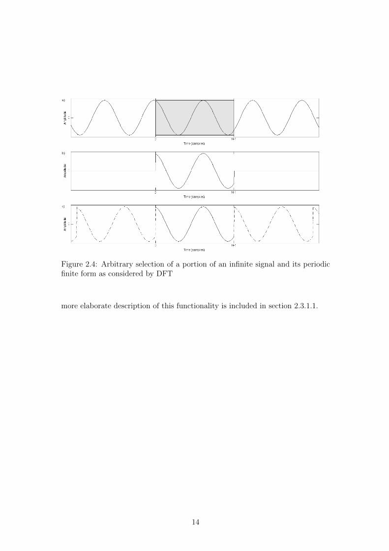
Figure 2.4: Arbitrary selection of a portion of an infinite signal and its periodicfinite form as considered by DFT

more elaborate description of this functionality is included in section 2.3.1.1.

14

Figure 2.5: The rectangular window and its spectrum

Figure 2.6: Illustration of the case where the amplitude spectral components of asignal coincide with the nulls of the sidebands of the amplitude spectrum of therectangular window function. The amplitude spectrum of the window functionhas been delineated with the help of zero padding

15

2.3.1.1 Windowing

It was described in the previous paragraph that the windowing of a signal and the

spectral convolution of the window’s spectrum with the signal’s spectrum are un-

avoidable. It was also discussed that the manifestation of spectral leakage can be

avoided with appropriate selection of the starting and ending points of the signal

in order to diminish discontinuities. Additional window functions were developed

to compromise with discontinuities. These window functions have weighted sam-

ple values that taper towards zero at the sides of the frame. Subsequently, they

force potential discontinuities towards zero.

The deficiency of these windowing functions, however, lies in the resolution

of their spectral lobes. The width of their spectral lobes is bigger than the width

of the spectral lobes of the rectangular windowing function, which results in less

accurate estimations of the frequency components that are responsible for the

height of the peak. Specifically, the spread of the main lobe is often of interest,

because it is the one that has the biggest contribution to the signal’s spectrum.

Two of the main topics that come with windowing were introduced so far;

spectral leakage and frequency resolution. The latter is a quality value that is

often considered in window picking. It is important to stress that there is no

‘best’ window function. Another quality measure that is usually considered is

the amplitude difference between the main and the first side-lobe. It is generally

true that the greater difference means less ‘blurring’ in the frequency domain.

Having introduced the main factors considered in the assessment of the suit-

ability of a window function, a few popular window functions along with their

parameters are listed for comparison in table 2.1. More window functions are

described in greater detail in Harris’ and Nuttall’s papers [13, 14].

The application of any window function other than the rectangular incurs

energy loss, since part of the signal’s amplitude is decreased. This results in loss

of information and data degradation. However, this is often exploited in STFT

depending on the application for which it is used. This is described in greater

detail in the following sub-section.

16

WindowFunction

Main-to-sidelobeamplitude difference (dB)

Main lobe width(sampled frequency

components)Rectangular -13 2Hamming -31 4Hann -41 4Blackman -57 6

Table 2.1: Specification of a few popular window functions

2.3.2 Short-Time Fourier Transform

The Short-Time Fourier Transform provides an insight on the frequency be-

haviour of a signal at certain points in time. This analysis method represents

the amplitude of the spectral components as a function of both frequency and

time. It achieves this by sliding a window along the signal and obtaining the

segment’s spectra. Every part of the signal that contributes one spectrum is

called frame m and it is of length L. The interval between successive frames is

determined by the step variable, H. The introduction of this variable allows the

overlap between successive frames. The total number of frames, M , obtained

from STFT depends on three factors; (1) the signal’s length N , (2) the frame

length L, and (3) the step size H. It is important to stress the discard of the last

frame in case it is incomplete.

Xm[k] ,L−1∑n=0

x[n]w[n− (m− 1)H]e−jϕk[n],k = 0, 1, . . . , L− 1

m = 1, 2, . . . ,M(2.20)

where

ϕk[n] = 2πfkn+ φ[0], n = 0, 1, . . . , L− 1 (2.21)

fk =k

N, k = 0, 1, . . . , L− 1 (2.22)

17

M = rounddown(N − (L−H)

L−H) (2.23)

The output of the STFT is the spectrogram, which is a 3D plot. A typical

representation includes the frames on the abscissa, the sampled frequencies on

the ordinate (or vice versa), and the spectral density as height. The spectrogram

is usually viewed from top as a 2D plot, where the time and frequency lie on the

x and y axis respectively. The energy density representation is achieved through

its mapping on a range of colours. An example spectrogram of a linear chirp is

portrayed in figure 2.7.

Figure 2.7: Spectrogram of a linear chirp sampled at 1024 Hz and total length1024 samples that starts at DC at sample 1 and crosses 0.5859 at sample 512.STFT parameters: frame length = 256, overlap = 75%, zpf = 0, window function= Hamming

The step variable, H, is responsible for the amount of overlap exhibited be-

tween successive frames. Setting the step size equal to the frame length, L, gives

0% overlap. Whereas, setting the step size to a quarter of the frame length equals

to 75% overlap. The following equation expresses the overlap in percentage with

18

respect to the frame length, L, and step size, H. In practice, percentages of

overlap greater than 0 result in time interpolation for analysis with rectangular

windowing function. This generates no new information, as it merely creates

more data points between the spectral values that would have been obtained in

the case of 0% overlap.

overlap(%) =L−HL

× 100 (2.24)

It is also possible to improve the resolution portrayed across the frequency

axis. This is achieved with zero padding1, which is a simple time-domain tech-

nique that has the effect of broadband time interpolation in frequency domain.

Zero padding is the introduction of a string of zeros at the end of every frame.

The size of this string is usually an integer multiple of the frame length, and is

calculated with the aid of the zero padding factor variable, zpf . The zpf indi-

cates the number of points introduced between the successive values that would

have been obtained with no zero padding. The introduction of zero padding in-

creases the number of samples considered within the FFT, and the total amount

of samples is determined by the following expression:

nfft = zpf · L, zpf = 1, 2, 3, . . . (2.25)

The STFT officially has no inverse function, although it can be defined for

particular cases. One of them is the case were 50% overlap and a window function

that tapers towards zero at the edges and reduces the energy of each frame to 50%

have been employed during the analysis stage. The reconstruction of the original

signal in time domain is achieved with the use of the overlap-add algorithm [15],

in order to preserve the energy. A couple examples of window functions that

taper towards zero at their edges and capture only 50% of the signals energy are

the Hamming and Hann.

1There are also alternative ways, such as interpolating directly the frequency values.

19

2.3.3 Discussion

2.3.3.1 DFT versus FFT

The development of an optimisation of the DFT function was discussed in 2.3.1,

the FFT. Its only prerequisite is the length of the signal under analysis to be

equal to a power of 2. This is not an issue in the context of this project, as there

are no constrains about the length of the signals considered. Thus, the FFT

algorithm is used in order to achieve lower computational expense.

2.3.3.2 Single-estimate versus Multiple-estimate Averaged Spectro-grams

The obtainment of a spectrum of lower variance, higher data credibility and re-

duced resolution has been suggested from Bartlett and Welch [16, 17, 18]. Both

Bartlett’s and Welch’s approaches involve the sectioning of the subject signal in

many frames, obtaining their spectra, and averaging their values. The difference

between the Bartlett’s and Welch’s spectra lies in the step size between the con-

secutive frames. Bartlett’s approach utilises 0% overlap, whereas Welch allows

50% overlap to be applied between the successive frames. These two approaches,

however, are not appropriate for the data with which this project deals, because

the averaging of the spectra deteriorates the resolution of the spectral peaks. The

frequency content of audio signals varies rapidly, and therefore, it is important to

not deteriorate the resolution. Thus, the single-estimate approach was utilised.

2.3.3.3 STFT parameter setting

There are many factors that require consideration prior to the analysis of a signal.

Every step and variable in the STFT algorithm introduces yet another layer of

complexity. It is important to carefully assess the available options in order to

optimise the output of this analysis method. As it has been thoroughly explained

in 2.3.1, the selection of the length of the signal alone may result in distorted

output information. It is, then, obvious that the inconsiderate setting of the

STFT parameters may incur significant inaccuracies on the signal’s spectra.

One of the most important matters for consideration is the time-frequency

resolution, which is fixed. This resolution is determined by the frame length, L,

20

and the sampling frequency of the signal, fs. So far this report has used nor-

malised examples, which means the sampling frequency was set to 1. In practice,

however, it is much greater than 1. For instance, the typical sampling frequency

used in most audio files is 44.100 Hz1. The expression that calculates the fre-

quency resolution of the sampled spectral components, which also happens to be

the lowest range of frequencies detected (fbin), is:

fbin =fsL

(2.26)

This indicates the range of frequencies that every sampled spectral component

represents (bandwidth). The frequency and time resolutions are associated to

the uncertainty principle, which was first observed by Heizenberg in quantum

physics. For STFT it means that longer frames result in better frequency reso-

lution, whereas shorter frames result in better temporal resolution. This effect

is depicted in figure 2.8. Furthermore, the product of the standard deviations

of the frequency and time elements of the spectrogram plane is always the same

constant.

Figure 2.8: Various time-frequency resolutions

1According to sampling theorem, this sampling frequency allows the representation of allaudible frequencies, having considered the necessary filtering applied at the high-end of thespectra, by the auditory system.

21

∆t∆f =1

4π(2.27)

It is important to consider the frame length prior to the analysis of a signal

for an additional reason. In his paper on the extraction of spectral peak parame-

ters, Depalle [19] states that components that exhibit less than 4 periods within

the frame result in considerable inaccuracies. The following table (2.2) trans-

lates what this statement means in terms of frame length and lowest frequency

component detected for fs = 44.100 Hz.

Frame length L (samples)Lowest accurately

detectable frequency (Hz)512 344.61024 172.32048 86.24096 43.18192 21.616384 10.8

Table 2.2: Lowest accurately estimated frequency with respect to different framelengths (based on [19])

Improving the time and frequency resolution with interpolation is also a mat-

ter of consideration. Although it is usually preferable to have more points because

of the aesthetically nicer portray, zero padding and high percentages of overlap

are not always an option. These functionalities are computationally expensive,

which might be undesired due to the already computationally expensive imple-

mentation of an algorithm. Therefore, careful thought must be given on the

advantages and disadvantages of these techniques prior to their employment.

2.3.3.4 Practical implementation of the STFT

Although the STFT description in 2.3.2 considers its functionality as a sliding

window along the signal, its practical implementation is different. In reality, the

STFT is calculated by sequentially considering a segmented portion of the signal

(frame m) of length L, and analysing it with the FFT. The rest of the parameters

22

remain the same. In terms of its equation, the only difference is the change of the

signal’s and window’s arguments. An example of the practical implementation of

the STFT is illustrated in figure 2.9, where the framed first quarter of the signal

analysed is included along with its spectrogram.

Xm[k] ,L−1∑n=0

x[n+ (m− 1)H]w[n]e−jϕk[n],k = 0, 1, . . . , L− 1

m = 1, 2, . . . ,M(2.28)

Figure 2.9: Illustration of the obtainment of a spectrogram with the practicalimplementation of STFT. The first quarter of the signal is depicted in a), whichis analysed with a Hamming window function (due to spectrogram function inMATLAB). N = 12288, L = 1024, H = 1024, zpf = 0

2.3.3.5 ISTFT

The ISTFT algorithm is defined here, since it is a vital part of the source sepa-

ration algorithm implemented by this project (see chapter 5). The overlap-add

method [15] is implemented in order to reconstruct the original signal in its tem-

poral form.

23

In the case of 0% overlap, the algorithm is straightforward. It merely trans-

forms each frame with IFFT and places it on the correct position. It is important

to stress that in the case where zero padding has been applied, only the first L

samples are kept.

x[(m− 1)L+ 1 : (m− 1)L+ L] ,∑nfft−1

k=0 Xm[k]e−jϕk[n]

n = 0, 1, . . . , nfft− 1, m = 1, 2, . . . ,M

(2.29)

In the case where 50% overlap has been applied, the algorithm is slightly

different. The calculation of the starting and ending points of the position of

each transformed frame are determined by the step variable, H. Again, if zero

padding has been applied, only the first L samples are kept.

x[(m− 1)H + 1 : (m− 1)H + L] ,∑nfft−1

k=0 Xm[k]e−jϕk[n]

n = 0, 1, . . . , nfft− 1 m = 1, 2, . . . ,M

(2.30)

2.3.4 STFT Modifications

The main limitation of the STFT, which is defined as soon as the analysis param-

eters are set, is the fixed time-frequency resolution. This limitation is directly

connected to the STFT’s (and implicitly the DFT’s) implementation, and is un-

avoidable. However, this is not the only issue. An additional matter that requires

attention is the lack of additional observations (estimations) in order to decrease

the variance and bias of the obtained results. This issue is also always present

but is much less considered in comparison to the limitations of the fixed grid.

These issues have been observed since very long ago (1970s), and various

approaches have been developed that attempt to tackle them. The three main

categories under which all STFT modifications can be catalogued are (1) mul-

tiresolution (which encompasses Adaptive STFT), (2) frequency reassignment,

and (3) multitapers. Although these have often been named differently, it will be

shown that despite the naming variations they share the same principles.

24

2.3.4.1 Multiresolution

Multiresolution for STFT-based algorithms is the calculation of the spectrum

of a signal with varying window sizes (frame length). This results in a grid

with unequally spaced tiles as it is portrayed in figure 2.10. The advantage of

this approach is the increased frequency resolution at certain bandwidths, while

maintaining the temporal resolution at other bandwidths. The main disadvan-

tages, excluding the computational expense, is the lack of an inverse function,

which precludes spectral processing.

Figure 2.10: Grid representation of a multiresolution approach

The concept of the computation of the spectra with unequal resolution was

first introduced by Oppenheim in 1971 [20]. In his paper, he mentioned that

the unequally spaced samples (tiles) correspond to a constant Q instead of be-

ing linearly related, and attempted to establish the fundamental principles that

allowed the implementation of this idea with the means they had available (non-

recursive and recursive filter banks). The term constant Q refers to the ratio of

the centre frequencies with the desired resolution, which is equal for all bins. In

terms of music analysis, the most popular constant Q modification was Brown’s

[21]. Her approach was embraced by music researchers better than other ap-

proaches that she mentions in her paper, because of the intuitive resolution her

algorithm utilises. This resolution maintains a good balance between musical and

perceptual viewpoints.

25

2.3.4.2 Adaptive STFT

The adaptive STFT (ASTFT) shares many principles with the multiresolution

techniques. Thus, it can be considered as a branch of the multiresolution time-

frequency analysis family. Similar to multiresolution techniques, ASTFT at-

tempts to circumvent the fixed time-frequency resolution. However, it follows

a slightly different approach. ASTFT analyses the data multiple times with

different frame lengths, and intelligently chooses the spectral coefficients that

exhibit the best signal representation, both temporally and spectrally. Unlike

multiresolution, it uses the homogenous axis of the highest resolution , but plots

a combination of the analysis coefficients of all analysis. A visual illustration of

the eventual result of this procedure is depicted in figure 2.11.

Figure 2.11: Grid representation of an ASTFT approach

The spectral coefficient combination can be achieved due to two constrains

set on the parameters of each analysis; (1) zero padding of the frames of all

analysis up to the frame length of the analysis with the biggest number of points

considered, and (2) overlapping at certain points in time, which are determined

by the overlap of the analysis with the smallest frame length. This results in the

obtainment of equal number of spectral coefficients that are accurately aligned in

time.

The ASTFT aims to decrease time and frequency smearing. Short frames

result in undistinguishable bass harmonics from the bass drum, while they main-

tain the temporal characteristics of the signal, whereas long frames result in time

26

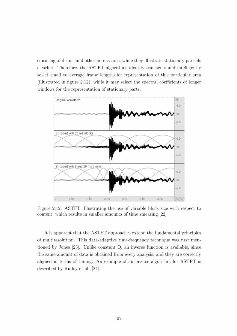
smearing of drums and other percussions, while they illustrate stationary partials

clearlier. Therefore, the ASTFT algorithms identify transients and intelligently

select small to average frame lengths for representation of this particular area

(illustrated in figure 2.12), while it may select the spectral coefficients of longer

windows for the representation of stationary parts.

Figure 2.12: ASTFT: Illustrating the use of variable block size with respect tocontent, which results in smaller amounts of time smearing [22]

It is apparent that the ASTFT approaches extend the fundamental principles

of multiresolution. This data-adaptive time-frequency technique was first men-

tioned by Jones [23]. Unlike constant Q, an inverse function is available, since

the same amount of data is obtained from every analysis, and they are correctly

aligned in terms of timing. An example of an inverse algorithm for ASTFT is

described by Rudoy et al. [24].

27

2.3.4.3 Frequency Reassignment

Frequency reassignment is a technique applied on the spectra after the STFT

analysis has been obtained, which attempts to provide more meaningful coordi-

nates for the spectral components [25]. Once the STFT has been obtained with a

fixed grid, the channelised instantaneous frequency (CIF) and local group delay

(LGD) parameters are calculated, which are the first derivatives of the complex

spectra with respect to time and frequency respectively. Then, the spectral com-

ponents are plotted at the points described by the estimated CIF and LGD, which

results in the reassigned spectrum of the signal.

This technique was first introduced by Kodera et al. [26] according to Fulop

and Fitz [25]. In their paper, Fulop and Fitz attempt to gather all the necessary

information about time-corrected instantaneous frequency (TCIF) analysis to es-

tablish a unified framework, and make information more accessible. They also

provide a few examples on the application of frequency reassignment. Addition-

ally, they provide more examples on speech and musical analysis in [27], where

they also include an explicit description of the algorithm.

Despite the greater localisation of the frequency components, both in time

and frequency, frequency reassigned spectra are very noisy. Meaningful results

are obtained around the neighbourhood of a component, while it might incur

random output at areas that contain no significant frequency components. A

de-noising method was proposed by Fulop and Fitz [27], inspired from empirical

observations. This method exploits the statistical behaviour that the 2nd deriva-

tive of the spectral coefficients manifests. Moreover, this technique is only used

for analysis, since the spectral components are arbitrarily placed, both in time

and frequency.

2.3.4.4 Multitapers

Multitapers approach the STFT from a different angle. From a statistical point

of view, the results of STFT lack validity, since the signal’s spectrogram is the

result of a single observation (estimation). The corresponding amplitude and

phase measures are not always correct due to the deficiencies of DFT, which

have been thoroughly examined in 2.3.1. Subsequently, the results are thought

28

to be biased and of great variance. This issue is tackled by multitapers, which

introduces multiple estimates for every frame.

Multitapers, first introduced by Thomson [28], and also named as multi-

window analysis in many papers [29, 30], is an approach that attempts to in-

crease the validity of the results and achieve higher credibility by obtaining more

than one measurement (transformation) for each frame. Every observation is

calculated with a different window function that is applied to the data, and the

final output is an average of the estimates obtained. The window functions are

all orthogonal to each other, and optimally concentrated in frequency. This was

judged to be necessary by Thomson in order to minimise the variance and the

bias of the estimates.

Pitton’s paper, named “Time-frequency spectrum estimation: An adaptive

multitaper method” [31], should not be confused with the adaptive as it is used

in the ASTFT. Pitton is following a different approach when he combines the

estimates for the obtainment of the spectrum. Instead of simple averaging, he

is intelligently weighting each observation with respect to a quality measure he

devised about the amount of spectral leakage they manifest.

2.3.5 Summary

This section has elaborated on the fundamentals of spectral processing by ex-

plaining the functionality of the STFT/DFT and its underlying technicalities,

and reviewed a number of modifications developed to compensate with the limi-

tations of STFT.

The ultimate STFT algorithm is envisioned as a combination of the modifi-

cations that were covered in 2.3.4, since the internal deficiencies that come with

the discrete implementation of the Fourier transform are inevitable. This version

of STFT should be adaptable, with unfixed time-frequency representation, whose

output will be credible due to the number of estimations obtained. Although this

idealistic product is far from what is currently available and it would require the

consideration of several factors (computational expensive), there are algorithms

that attempt to marry multiple modifications of STFT, as described in 2.3.4.

More specifically, Xiao et al. [32] have developed a hybrid modification of STFT

29

that combines multitapers with frequency reassignment. Although at very early

stages, it seems that the evolution of STFT is heading this way.

Despite the fact that the available modifications of the STFT attempt to tackle

most of its limitations, there is no modification that deals with the arbitrary

selection of the starting and ending points of each frame. It was shown in 2.3.1

that this can incur considerable amounts of spectral leakage. Also, the lack of

interest in the phase information obtained from the spectral analysis technically

results in incomplete analysis of the data. To the best of the authors knowledge,

there is no modification of the STFT that exploits phase information for the

improvement of the credibility of the analysed data. It is understandable that

phase might not be meaningful or coherent for signals in various fields, however, it

can be for audio signals. The following chapter focuses on the research conducted

in an attempt to address the aforementioned issues.

30

Chapter 3

Phase Stability Quality Measure

Fourier techniques are plagued with a variety of assumptions and user-specific

design choices, which result in a number of compromises.

• The foremost inevitable assumption is the stationarity of every framed sig-

nal considered by Fourier approaches. This often results in incoherent data,

since the varying frequency content of non-stationary signals is interpreted

as separate frequency components.

• Moreover, the arbitrary partition of the signal into frames in the STFT,

whose starting and ending points are determined by fixed offsets with re-

spect to the data start point, often results in edge effects, which also dete-

riorate the credibility of the data (described in 2.3.1).

In addition, a set of user-specific design choices require determination in

STFT, which result in further compromises. A detailed description of the user-

specific design choices can be found in 2.3.3.3 but a summary is provided in the

table 3.1, where each choice is linked to its subsequent compromise.

Numerous techniques have been developed that attempt to compensate the

deficiencies of the STFT (see 2.3.4). They, however, focus on the issues that are

described in table 3.1 (with the exception of the discard of phase information),

leaving the list of issues as described by the bullet points unaddressed. A rel-

atively simple concept is proposed of a different mindset to those described in

2.3.4 that attempts to address these issues. The aim of this novel modification

31

Frame length -Time vs.frequency resolution

Window function -Spectral leakage vs.peak bandwidth

Overlap -Temporal interpolationvs. computational expense

Points considered by FFT(> frame length,

if zero padding is applied)-

Frequency interpolationvs. computational expense

Discardof phase information

Table 3.1: User-specific design choices of STFT and their implications

of STFT is to improve the quality and credibility of the estimated results for the

analysis of stationary or near-stationary digital signals.

3.1 Motivation: PASS with EASE

This work is based on some unpublished initial studies carried out by the project

supervisor [33]. These studies focus on the development of an ensemble of estima-

tions in order to compensate some of the artefacts that arise due to discontinuities.

This approach also indicated that the phase content of a signal could carry useful

information. The earlier work, however, was neither fully tested nor applied to

any specific signal processing application. This project extends this initial stud-

ies with the development of a function that utilises phase information to define a

confidence level for the estimated data, and applies it in the framework of source

separation to assess its suitability and effectiveness.

3.2 Research Hypothesis, Aims and Objectives

It is hypothesised that the phase information for a sampled frequency com-

ponent arising from a partial observed at sufficiently small intervals manifests

structure which distinguishes it from phase information due to noise or Fourier-

related artefacts. This can then be exploited in order to obtain a confidence level

that can be attached to every frequency bin of the estimated spectrum, and pro-

32

duce the enhanced spectra of the signal. The end result is anticipated to be more

credible and of better quality, since it should be easier to discriminate between

“structure” and “noise” or “artefacts”.

The novelty of this work lies on the use of ensembles of STFT estimates

obtained around the area of the original starting point of the frame instead of a

single observation for every arbitrarily selected frame. In addition, the use of the

phase information in a meaningful fashion for the improvement of the credibility

of the data differentiates this approach from the available STFT modifications.

The aim of this research was the implementation, testing and validation of

this novel approach, the definition of the measure that will act as a confidence

level for every individual bin, and its employment in the framework of source

separation in order to assess its effectiveness (chapter 5).

The development of this project was achieved with the attainment of the

following objectives:

1. Investigation of the phase behaviour of simple synthetic signals and the

initial phase angles obtained from an STFT approach.

2. Development of the analysis tool and the necessary underlying functions.

3. The testing of this method on a set of signals in order to validate its func-

tionality.

4. Evaluation of the developed functionality with its incorporation in an exam-

ple application (chapter 5) and consolidation of a list of aims for attainment

in the future (chapter 7).

3.3 Principles

A set of simple synthetic signals, both stationary and non-stationary, are em-

ployed in this section to introduce the methodology proposed, illustrate the po-

tential of the ensemble of closely-related estimates approach, and define the phase

stability quality measure. The length of the signals and the number of additional

estimates were kept small to allow the portrayal of all relevant information.

33

3.3.1 Stationary Signals

An idealised cosine signal is considered in this sub-section.

y(t) = cos(ϕ(t)) (3.1)

ϕ(t) = ωt+ φ(0) (3.2)

The cosine, which is comprised of 128 samples in total, with a single period

containing 16 samples, is depicted in figure 3.1. In addition, the wrapped phase

coefficients of the cosine that are plotted against time and the amplitude spectrum

of the signal are provided and serve as a reference points. They allow comparisons

to be made between the phase and amplitude spectrum behaviour of the original

signal and the following framed signals.

Consider the application of an arbitrary frame on the cosine and 3 additional

frames of high overlap with respect to the first frame to obtain the ensemble of

closely-related estimates, with the application of rectangular window functions.

The additional 3 frames are required in order to obtain the short-time evolution

of the phase behaviour of the signal. The first frame is thought to be the original

as applied by STFT, and the rest 3 are the additional estimates as suggested by

this project’s approach. Therefore, each frame is named after the number of the

original frame and the number of estimate, i.e. for frame 1, the 6th estimate is

called Frame 1.6. Setting the frame length to 41 samples and a relatively short

sample shift for every additional estimate, 2 samples (corresponds to π8

shift in

phase in the particular example), results into the scenario illustrated in figure

3.2. The figures 3.3 and 3.4 accompany figure 3.2, and depict the subsequent

periodic wrapped phase behaviour of the framed signal as considered by FFT,

and its actual logarithmic amplitude spectrum in order to showcase the spectral

leakage levels.

Frame 1.1 of figure 3.2 is the frame that manifests the greatest degree of

edge discontinuity. The selected portion of the signal starts at the maximum

value and ends at the minimum. This discontinuity is expected to result in large

34

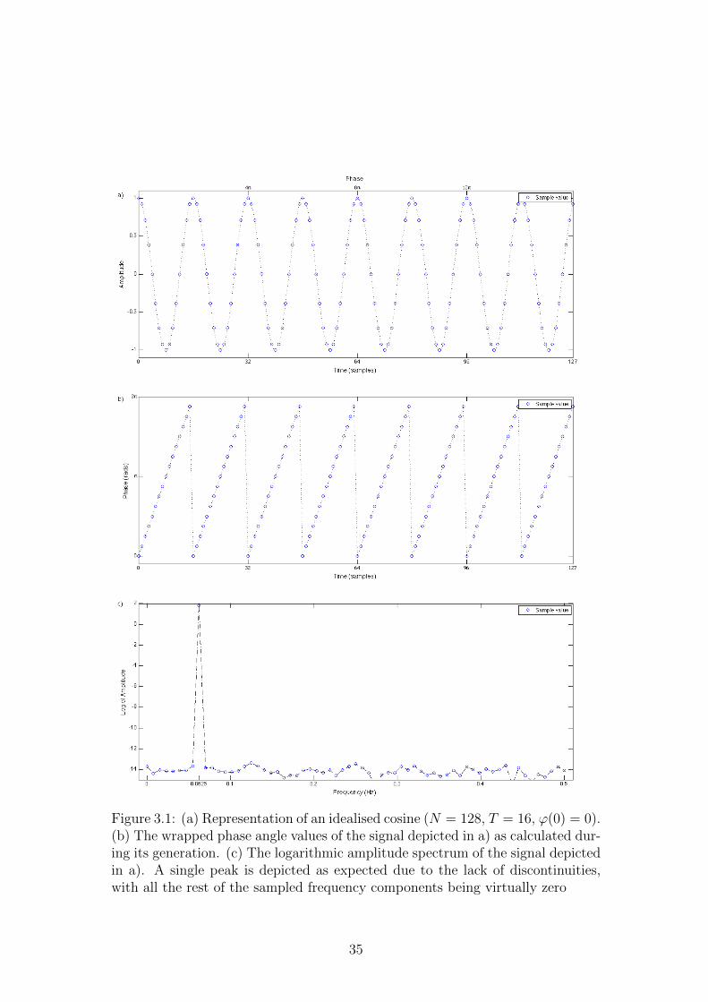
Figure 3.1: (a) Representation of an idealised cosine (N = 128, T = 16, ϕ(0) = 0).(b) The wrapped phase angle values of the signal depicted in a) as calculated dur-ing its generation. (c) The logarithmic amplitude spectrum of the signal depictedin a). A single peak is depicted as expected due to the lack of discontinuities,with all the rest of the sampled frequency components being virtually zero

35

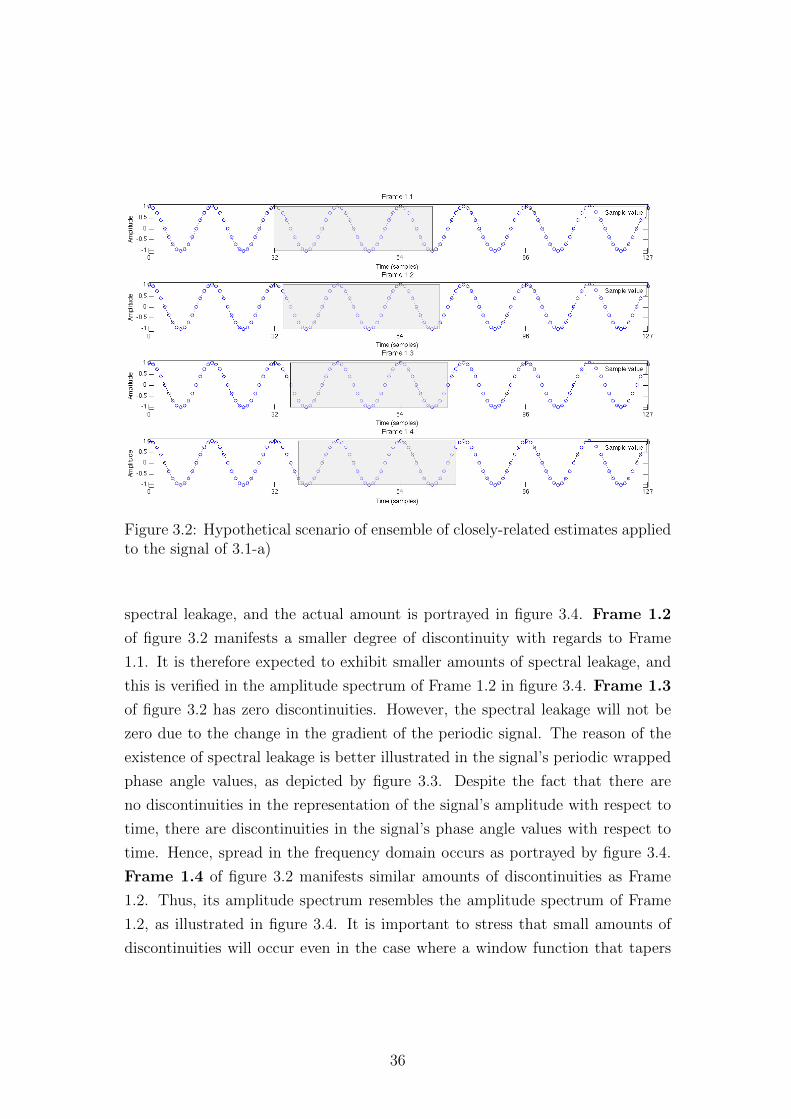
Figure 3.2: Hypothetical scenario of ensemble of closely-related estimates appliedto the signal of 3.1-a)

spectral leakage, and the actual amount is portrayed in figure 3.4. Frame 1.2

of figure 3.2 manifests a smaller degree of discontinuity with regards to Frame

1.1. It is therefore expected to exhibit smaller amounts of spectral leakage, and

this is verified in the amplitude spectrum of Frame 1.2 in figure 3.4. Frame 1.3

of figure 3.2 has zero discontinuities. However, the spectral leakage will not be

zero due to the change in the gradient of the periodic signal. The reason of the

existence of spectral leakage is better illustrated in the signal’s periodic wrapped

phase angle values, as depicted by figure 3.3. Despite the fact that there are

no discontinuities in the representation of the signal’s amplitude with respect to

time, there are discontinuities in the signal’s phase angle values with respect to

time. Hence, spread in the frequency domain occurs as portrayed by figure 3.4.

Frame 1.4 of figure 3.2 manifests similar amounts of discontinuities as Frame

1.2. Thus, its amplitude spectrum resembles the amplitude spectrum of Frame

1.2, as illustrated in figure 3.4. It is important to stress that small amounts of

discontinuities will occur even in the case where a window function that tapers

36

Figure 3.3: The periodic version of the wrapped phase angle values of the framedsignals depicted in figure 3.2, as considered by FFT

Figure 3.4: The logarithmic amplitude spectra of the framed signals of figure 3.2

37

to zero towards the edges is applied.

According to the amplitude spectra of the closely-related estimates as illus-

trated by figure 3.4, the bins that exhibit significant presence of a frequency

component and preserve their amplitude approximately on the same levels are

in the area of (0.03 − 0.1 Hz). It is known from the specifications of the signal

that its frequency lies within this area (T = 16, hence f =1

T= 0.0625). In

contrary, the amplitude of the rest of the bins vary greatly with regards to every

shifted estimate. Respectively, these are the bins that they do not relate to the

frequency of the signal component, and can be thought as the bins that arise

from algorithmic artefacts, specifically spectral leakage in this case.

Having examined the amplitude behaviour, attention is now focused on phase

and its variance with respect to frame position. Specifically, the sets of initial

phase angle values of two bins is investigated, one from the neighbourhood of

the frequency component and one from the spectral leakage neighbourhood. The

complete set of initial phase angle values obtained by FFT is included in Appendix

A on page 93, but the values of the two representative bins are copied in table

3.2. Moreover, a graph is plotted (figure 3.5) holding the values of each frame

sequentially in order to make their observation easier.

Frame 1.1Initial phase

(rads)


(rads)


(rads)


(rads)Bin 4 -1.341 -0.636 0.230 1.096Bin 18 -0.268 -0.214 1.303 2.819

Table 3.2: Initial phase for every frame estimate for bin 4 and 18

Figure 3.5 reveals interesting results. The phase values of the bin that holds

significant part of the frequency component’s energy are a linear function of the

shift number. On the other hand, the coefficients of the bin that occurs due to

spectral leakage exhibit some degree of randomness. This information is then

exploited in order to produce a quality measure for each bin.

A 1st order curve is fitted to the data, which represents the behaviour of the

phase of a stable frequency component (equation 3.2). Figure 3.6 portrays the

modelled phase values of the idealistic frequency component against the actual

38

Figure 3.5: Initial phase angle value variation for each estimate, as obtained fromFFT, for bins 4 and 18

values obtained by FFT in order to illustrate their difference. Then, the deviation

of the initial phase values obtained by FFT from the modelled data is calculated

in order to find the deviation of the actual measurement from the behaviour

of an idealistic frequency component (portrayed in figure 3.7-a & b). Finally,

calculating the least squares of the deviation of the phase values from the 1st order

curve results in the measure that indicates the variance of the actual frequency

component as perceived by FFT from an idealistic frequency component. This

measure is here defined as the phase stability.

39

Figure 3.6: Initial phase angle value variation for each estimate as obtained fromFFT against the modelled phase angle values of an idealistic frequency componentfor two representative bins

Figure 3.7: (a) Deviation of the phase values calculated by FFT from the modelledphase values of an idealistic frequency component for bin 4. (b) Deviation of thephase values calculated by FFT from the modelled phase values of an idealisticfrequency component for bin 18. (c) Phase Stability: The sum of the least squaresof the deviation for each bin

40

3.3.2 Non-Stationary Signals

The behaviour of a near-stationary signal and a non-stationary signal is examined

in this section. These signals have been tailored to represent common realistic

musical effects that are often incorporated in musical performances. The aim is to

investigate the performance of the ensemble of closely-related estimates approach

and the phase behaviour with regards to the frame shift on these cases of greater

complexity where conventional Fourier techniques are inadequate.

1. The first signal contains the same cosine examined in the previous section

but with vibrato applied on it.

y(t) = cos(ϕ(t)) (3.3)

ϕ(t) = Asin(ωvt) + ωct+ φ(0) (3.4)

The signal is 128 samples long, with centre frequency of fc = 0.0625 Hz.

A typical vibrato effect may vary the centre frequency by two semitones.

Thus, in order to find the interval of a semitone, an octave was devised with

starting note at 0.0625 Hz and ending at 0.125 Hz. It was then divided into

12 equal intervals, which unveiled the value of a semitone, Av = 0.0057

(Hz deviation from fc). Thus, the end result varied between 0.0568 Hz

and 0.0682 Hz four times in the span of these 128 samples (fv = 32 Hz)

(figure 3.8-a). The particular vibrato frequency was found appropriate for

illustrative purposes, although it differs largely with respect to realistic

vibrato rates.

2. The second signal represents a frequency sweep (chirp), which corresponds

to the glissando effect.

y(t) = cos(ϕ(t)) (3.5)

41

ϕ(t) = gπt2 + ωt+ φ(0) (3.6)

g =f1 − f0t1

(3.7)

where g is the chirp rate.

Glissandos may start at a note and terminate at the same note an octave

above. Therefore, the frequency of the subject signal starts at f0 = 0.0625

Hz and progresses linearly to f1 = 0.125 Hz in the span of the 128 samples

(figure 3.9-a)

The wrapped phase angle values as calculated during the generation of the

signals, and the amplitude spectra of the signals are provided in addition to

their temporal representations (figure 3.8-b & c, figure 3.9-b & c). Moreover, the

unwrapped phase angle values as calculated during the generation of the signals

are provided to demonstrate that these cases also exhibit trends (figure 3.10 &

3.11).

42

Figure 3.8: (a) Representation of the idealised cosine with vibrato. (b) Thewrapped phase angle values of the signal depicted in a) as calculated during itsgeneration. (c) The logarithmic amplitude spectrum of the signal depicted in a)

43

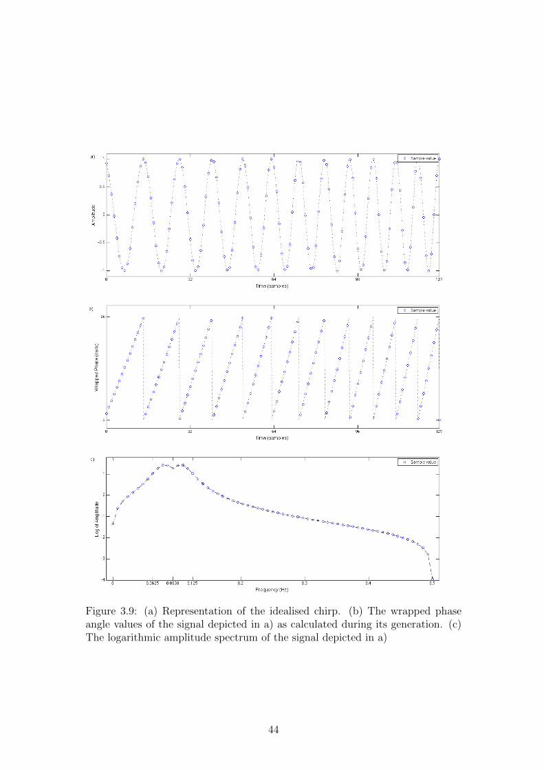
Figure 3.9: (a) Representation of the idealised chirp. (b) The wrapped phaseangle values of the signal depicted in a) as calculated during its generation. (c)The logarithmic amplitude spectrum of the signal depicted in a)

44

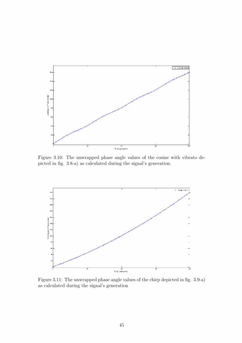
Figure 3.10: The unwrapped phase angle values of the cosine with vibrato de-picted in fig. 3.8-a) as calculated during the signal’s generation.

Figure 3.11: The unwrapped phase angle values of the chirp depicted in fig. 3.9-a)as calculated during the signal’s generation

45

The signals were subjected to four frames, as it was illustrated in figure 3.2 in

sub-section 3.3.1, and the amplitude spectrum of each frame was calculated with

FFT. The initial phase angle values of each analysis are included in Appendix B

& C, pages 94 and 95. Attention is focused on the same bins that were examined

in the previous example for the signal with vibrato, bin 4 and 18, whereas bin

8 and 18 are examined for the example with glissando due to the fact that bin

4 does not hold a significant component for the frequency sweep example (figure

3.9-c). Table 3.3 contains the phase values of the aforementioned bins for each

analysed frame of the signal with vibrato, whereas table 3.4 contains the phase

values of the signal with glissando.


(rads)


(rads)


(rads)


(rads)Bin 4 -0.657 0.195 1.063 1.759Bin 18 -0.221 0.567 2.816 2.878

Table 3.3: Initial phase angle values for bin 4 and 18 for the cosine with vibrato


(rads)


(rads)


(rads)


(rads)Bin 8 1.517 2.220 -3.077 -1.368Bin 18 2.761 2.890 3.135 2.8191

Table 3.4: Initial phase angle values for bin 8 and 18 for the chirp

Plotting the initial phase angle values sequentially for each bin reveals similar

results to the results obtained for the stationary signal (figure 3.12 represents the

vibrato signal, and figure 3.14 represents the chirp). The initial phase angle values

of the bins that contain a significant part of the subject signal are a function of

the shift number. Unlike with the stationary signal, the values are not linearly

related. Non-stationary signals that represent realistic musical performance styles

are best described with a second order curve.

1One π added to the original value for continuation purposes.

46

Figure 3.12: Phase coefficients as obtained from FFT for the cosine with vibratoagainst the modelled phase values of an idealistic frequency component

Figure 3.13: (a) Deviation of the actual phase values calculated by FFT from themodelled phase values of an idealistic frequency component with vibrato for bin4. (b) Deviation of the actual phase values calculated by FFT from the modelledphase values of an idealistic frequency component with vibrato for bin 18. (c)Phase Stability: The sum of the least squares of the deviation for each bin

47

Figure 3.14: Phase coefficients as obtained from FFT for the chirp against themodelled phase values of an idealistic frequency component

Figure 3.15: (a) Deviation of the actual phase values calculated by FFT from themodelled phase values of an idealistic frequency sweep for bin 8. (b) Deviation ofthe actual phase values calculated by FFT from the modelled phase values of anidealistic frequency sweep for bin 18. (c) Phase Stability: The sum of the leastsquares of the deviation for each bin.

48

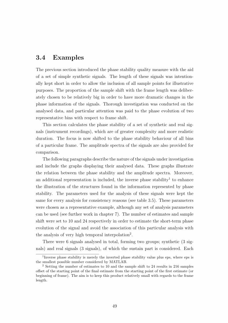
3.4 Examples

The previous section introduced the phase stability quality measure with the aid

of a set of simple synthetic signals. The length of these signals was intention-

ally kept short in order to allow the inclusion of all sample points for illustrative

purposes. The proportion of the sample shift with the frame length was deliber-

ately chosen to be relatively big in order to have more dramatic changes in the

phase information of the signals. Thorough investigation was conducted on the

analysed data, and particular attention was paid to the phase evolution of two

representative bins with respect to frame shift.

This section calculates the phase stability of a set of synthetic and real sig-

nals (instrument recordings), which are of greater complexity and more realistic

duration. The focus is now shifted to the phase stability behaviour of all bins

of a particular frame. The amplitude spectra of the signals are also provided for

comparison.

The following paragraphs describe the nature of the signals under investigation

and include the graphs displaying their analysed data. These graphs illustrate

the relation between the phase stability and the amplitude spectra. Moreover,

an additional representation is included, the inverse phase stability1 to enhance

the illustration of the structures found in the information represented by phase

stability. The parameters used for the analysis of these signals were kept the

same for every analysis for consistency reasons (see table 3.5). These parameters

were chosen as a representative example, although any set of analysis parameters

can be used (see further work in chapter 7). The number of estimates and sample

shift were set to 10 and 24 respectively in order to estimate the short-term phase

evolution of the signal and avoid the association of this particular analysis with

the analysis of very high temporal interpolation2.

There were 6 signals analysed in total, forming two groups; synthetic (3 sig-

nals) and real signals (3 signals), of which the sustain part is considered. Each

1Inverse phase stability is merely the inverted phase stability value plus eps, where eps isthe smallest possible number considered by MATLAB.

2 Setting the number of estimates to 10 and the sample shift to 24 results in 216 samplesoffset of the starting point of the final estimate from the starting point of the first estimate (orbeginning of frame). The aim is to keep this product relatively small with regards to the framelength.

49

Parameter Name ValueFrame length 4096Overlap 50%Zero paddingFactor

0

Window function HammingNumber of estimates 10Sample shift 24

Table 3.5: Phase stability analysis parameters for the analysis of the signals

group contained a stationary, a near-stationary (vibrato), and a non-stationary

(glissando) signal. All signals were comprised of multiple partials. Their length

was 1 second long and the sampling frequency was 44100 Hz. The graphs that

portray the analysed data of the synthetic signals display the second frame of

their analysis, which was arbitrarily selected. For the representation of the real

signals, however, the tenth frame is illustrated, which corresponds to the analysis

of the sustain part of the note.

The specification of the synthetic signals are described in the following list.

1. The first synthetic signal was comprised of four stationary frequency com-

ponents of [200 450 800 1300] Hz and amplitudes [0.2 0.1 0.03 0.08], respec-

tively.

2. The second synthetic signal was comprised of three partials of centre fre-

quency [300 800 1800] that each one deviates from the centre frequency by

20 Hz at a rate of 4 Hz. Their corresponding amplitudes are [0.2 0.1 0.5].

3. The synthetic signal with glissando consisted of three partials, starting at

[100 450 1100] Hz and terminating at [200 900 2200] Hz within the 1 second,

with amplitudes [0.2 0.1 0.5].

The real instrument recording was an A4 violin note obtained from the Music

Instrument Samples library of the University of Iowa [34]. The vibrato and glis-

sando effects were applied to the note artificially in Cubase 7.5 in order to know

the exact parameters of the signals. For the signal with vibrato, the pitch deviates

by 1 semitone from the original pitch at a rate of 5 Hz, and the processing with

50

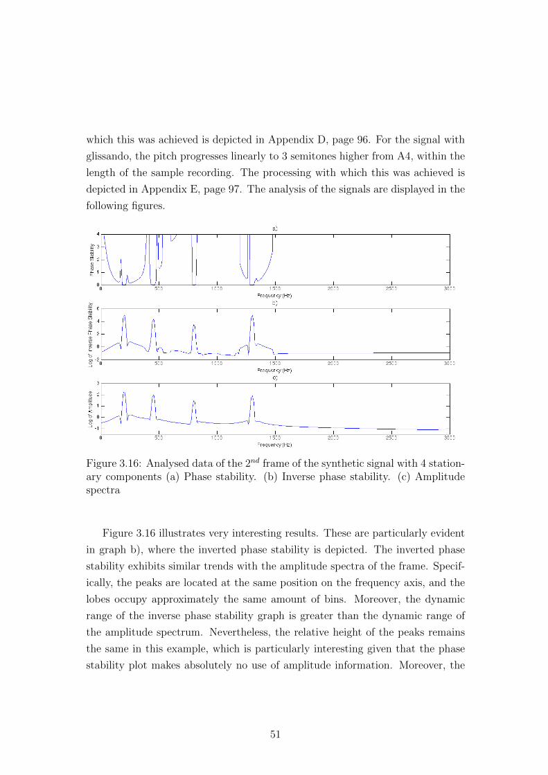
which this was achieved is depicted in Appendix D, page 96. For the signal with

glissando, the pitch progresses linearly to 3 semitones higher from A4, within the

length of the sample recording. The processing with which this was achieved is

depicted in Appendix E, page 97. The analysis of the signals are displayed in the

following figures.

Figure 3.16: Analysed data of the 2nd frame of the synthetic signal with 4 station-ary components (a) Phase stability. (b) Inverse phase stability. (c) Amplitudespectra

Figure 3.16 illustrates very interesting results. These are particularly evident

in graph b), where the inverted phase stability is depicted. The inverted phase

stability exhibits similar trends with the amplitude spectra of the frame. Specif-

ically, the peaks are located at the same position on the frequency axis, and the

lobes occupy approximately the same amount of bins. Moreover, the dynamic

range of the inverse phase stability graph is greater than the dynamic range of

the amplitude spectrum. Nevertheless, the relative height of the peaks remains

the same in this example, which is particularly interesting given that the phase

stability plot makes absolutely no use of amplitude information. Moreover, the

51

amplitude spectrum appears slightly smoother than the inverse phase stability

graph.

Figure 3.17: Analysed data of the 2nd frame of the synthetic signal with 3 near-stationary components (signal with vibrato). (a) Phase stability. (b) Inversephase stability. (c) Amplitude spectra

Similar results were obtained for the analysis of the stationary component

with vibrato, which can be seen in figure 3.17. The behaviour of the inverse

phase stability resembles the behaviour of the amplitude spectrum, with the

peaks located at the same place, occupying the same amount of bins. In this

example, however, the second lobe is much better defined by the inverse phase

stability. Again, the dynamic range is greater in the inverse phase stability than

the amplitude spectrum. Graph b) differs from graph c), however, towards the

high-end of the frequency axis where there seems to be a rise on the curve, which

does not exist in the amplitude spectrum.

52

Figure 3.18: Analysed data of the 2nd frame of the synthetic signal with 3 non-stationary components (signal with glissando). (a) Phase stability. (b) Inversephase stability. (c) Amplitude spectra

More noticable are the differences between the inverse phase stability and

the amplitude spectrum for the analysis of the synthetic example with glissando

effect. As with the previous examples, the inverse phase stability manifests similar

trends to the amplitude spectrum of the signal, and the lobes are approximately

of the same width. Also, the dynamic range of the graph that holds the inverse

phase stability is greater than the amplitude spectrum. However, the third lobe

exhibits interesting trends. The main peak is of the same width with respect to

the amplitude spectrum but there is an unexplainable increased activity around

it, which appears to be flat, that ends abruptly.

53

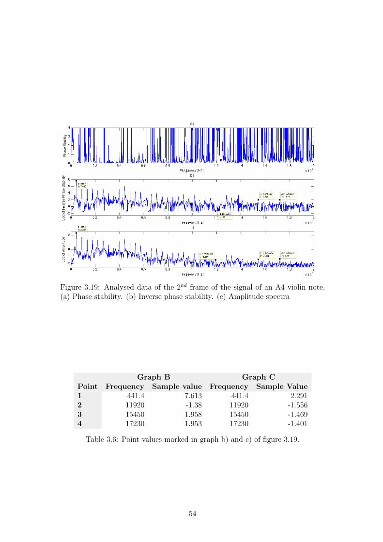
Figure 3.19: Analysed data of the 2nd frame of the signal of an A4 violin note.(a) Phase stability. (b) Inverse phase stability. (c) Amplitude spectra

Graph B Graph CPoint Frequency Sample value Frequency Sample Value1 441.4 7.613 441.4 2.2912 11920 -1.38 11920 -1.5563 15450 1.958 15450 -1.4694 17230 1.953 17230 -1.401

Table 3.6: Point values marked in graph b) and c) of figure 3.19.

54

Figure 3.19 is the first illustration of the behaviour of the phase stability (and

inverse phase stability) of real signals. The inverse phase stability graph appears

to manifest similar trends to the amplitude spectrum of the signal, where almost

all peaks can be spotted in both representations with the exception of the peak at

11920 Hz. The dynamic range of the inverse phase stability appears to be three

times greater than the dynamic range of the amplitude spectrum. The roll off of

the high frequencies of the inverse phase stability graph is considerably smaller

than the roll off of the amplitude spectrum. Having located the fundamental,

a few points were highlighted in the graphs that are thought to be harmonics,

whose values can be found in table 3.6.

55

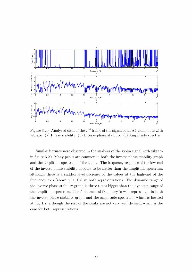
Figure 3.20: Analysed data of the 2nd frame of the signal of an A4 violin note withvibrato. (a) Phase stability. (b) Inverse phase stability. (c) Amplitude spectra

Similar features were observed in the analysis of the violin signal with vibrato

in figure 3.20. Many peaks are common in both the inverse phase stability graph

and the amplitude spectrum of the signal. The frequency response of the low-end

of the inverse phase stability appears to be flatter than the amplitude spectrum,

although there is a sudden level decrease of the values at the high-end of the

frequency axis (above 8000 Hz) in both representations. The dynamic range of

the inverse phase stability graph is three times bigger than the dynamic range of

the amplitude spectrum. The fundamental frequency is well represented in both

the inverse phase stability graph and the amplitude spectrum, which is located

at 453 Hz, although the rest of the peaks are not very well defined, which is the

case for both representations.

56

Figure 3.21: Analysed data of the 2nd frame of the signal of an A4 violin notewith glissando. (a) Phase stability. (b) Inverse phase stability. (c) Amplitudespectra

Graph B Graph CPoint Frequency Sample value Frequency Sample Value1 463 6.439 463 2.2682 7020 -3.091 7020 0.063 11680 1.347 11680 -0.84864 14020 1.464 14020 -1.028

Table 3.7: Point values marked in graph b) and c) of figure 3.21

57

Finally, the results of the analysis for the violin signal with glissando are de-

picted in figure 3.21. The inverse phase stability and amplitude spectrum manifest

similar trends, where it appears they have many peaks in common. The frequency

response of the inverse phase stability graph is not much flatter in comparison to

the frequency response of the amplitude spectrum. However its dynamic range is

greater than the dynamic range of the amplitude spectrum. Having located the

fundamental, 463 Hz, which is clearly depicted in both the inverse phase stability

and the amplitude spectrum, a few other peaks were highlighted that are consid-

ered to be harmonics. These peaks manifest a significant degree of prominence

in their neighbourhood.

3.5 Summary

The potential of the ensemble of closely-related estimates and the phase stability

quality measure have been investigated in this chapter. This approach circum-

vents a number of deficiencies that plague the conventional STFT approaches,

and provides more credible results. Specifically, it provides an additional insight

to the data, which also allows the incorporation of non-stationarity. A few anal-

ysis examples were provided, both synthetic and real signals, where interesting

results were obtained. Specifically, with the aid of the inverse phase stability, it

was found that the phase stability generally exhibits smaller roll off of the sample

values towards the high end of the frequency axis and has greater dynamic range

than the amplitude spectrum.

The two following chapters focus on the development of the function that im-

plements this approach and the application of the phase stability quality measure

in the framework of source separation.

58

Chapter 4

PhiStab Function

The development of the function that calculates the phase stability quality mea-

sure was achieved in two steps:

1. Modification of the conventional STFT algorithm in order to enable it to

construct the ensemble of estimates.

2. Processing of the data acquired from the modified STFT function to deter-

mine the phase stability quality measure for every bin of the spectra.

This chapter provides a thorough description of the steps carried out for the

implementation of the two objectives described in the previous bullet points. At

first, the development of the STFT modification is documented, followed by the

implementation of the method that calculates the phase stability quality measure.

Finally, the testing conducted on the newly developed functions is described.

4.1 STFT Modification: Construction of the en-

semble of estimates

The implementation of the methodology that produces the ensemble of closely-

related estimates in 3.3.1 and 3.3.2 requires the introduction of two additional

variables. These variables are (1) the number of estimates calculated for each

original frame (including the estimate of the conventional STFT), Q, and (2)

the corresponding sample shift of the frame for every estimate, C. These were

59

then incorporated into the conventional STFT algorithm in order to successfully

extend its functionality and enable it to construct the ensemble of estimates.

The first thing that required modification was the formula that determines the

number of frames in which the signal is segmented (see eq. 2.23). The discard of

the last incomplete frame for the conventional implementation of the STFT was

considered. This feature is also embodied in the modified version of the STFT,

which requires (Q−1) ·C additional samples for the construction of the ensemble

of estimates for the last frame. The modified formula that incorporates the two

new variables and calculates the number of frames is:

M = rounddown(N − (Q− 1) · C − (L−H)

L−H), 1 < H ≤ L (4.1)

The pseudo code of the practical implementation of the conventional STFT

algorithm is introduced in order to highlight the turn with which events occur.

Then, the additional steps that are required for the implementation of the en-

semble of estimates approach are defined and incorporated in the pseudo code

of the conventional STFT algorithm, which results in the desired modification of

the STFT.

The practical implementation of the STFT algorithm is described by eq. 2.28.

This equation is copied here (eq. 4.2) to allow comparisons to be made with the

modified version.

Xm[k] ,L−1∑n=0

x[n+ (m− 1)H]w[n]e−jϕk[n],k = 0, 1, . . . , L− 1

m = 1, 2, . . . ,M(4.2)

This equation can be translated into the following:

60

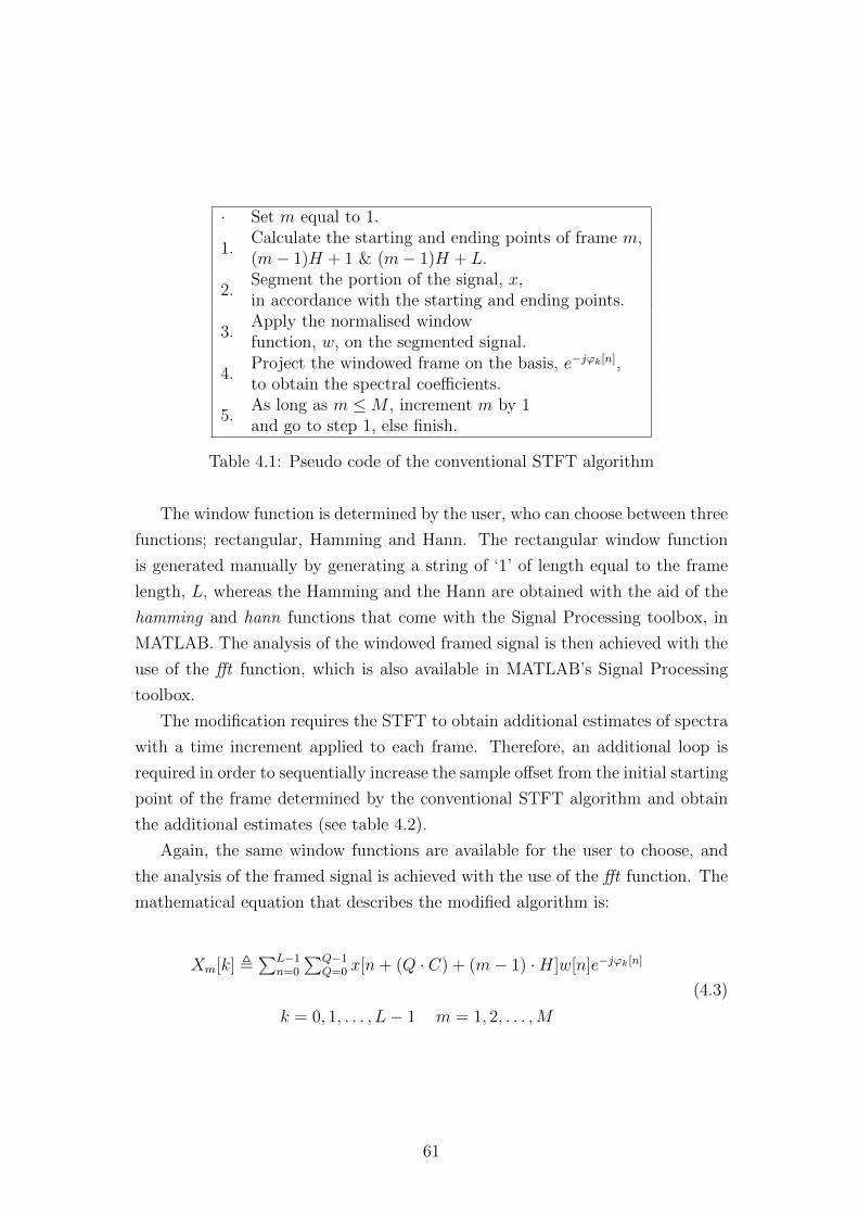
· Set m equal to 1.

1.Calculate the starting and ending points of frame m,(m− 1)H + 1 & (m− 1)H + L.

2.Segment the portion of the signal, x,in accordance with the starting and ending points.

3.Apply the normalised windowfunction, w, on the segmented signal.

4.Project the windowed frame on the basis, e−jϕk[n],to obtain the spectral coefficients.

5.As long as m ≤M , increment m by 1and go to step 1, else finish.

Table 4.1: Pseudo code of the conventional STFT algorithm

The window function is determined by the user, who can choose between three

functions; rectangular, Hamming and Hann. The rectangular window function

is generated manually by generating a string of ‘1’ of length equal to the frame

length, L, whereas the Hamming and the Hann are obtained with the aid of the

hamming and hann functions that come with the Signal Processing toolbox, in

MATLAB. The analysis of the windowed framed signal is then achieved with the

use of the fft function, which is also available in MATLAB’s Signal Processing

toolbox.

The modification requires the STFT to obtain additional estimates of spectra

with a time increment applied to each frame. Therefore, an additional loop is

required in order to sequentially increase the sample offset from the initial starting

point of the frame determined by the conventional STFT algorithm and obtain

the additional estimates (see table 4.2).

Again, the same window functions are available for the user to choose, and

the analysis of the framed signal is achieved with the use of the fft function. The

mathematical equation that describes the modified algorithm is:

Xm[k] ,∑L−1

n=0

∑Q−1Q=0 x[n+ (Q · C) + (m− 1) ·H]w[n]e−jϕk[n]

k = 0, 1, . . . , L− 1 m = 1, 2, . . . ,M

(4.3)

61

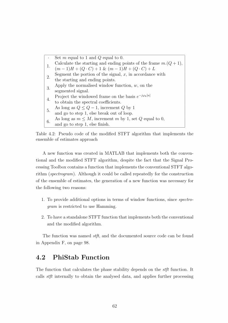
· Set m equal to 1 and Q equal to 0.

1.Calculate the starting and ending points of the frame m.(Q+ 1),(m− 1)H + (Q · C) + 1 & (m− 1)H + (Q · C) + L

2.Segment the portion of the signal, x, in accordance withthe starting and ending points.

3.Apply the normalised window function, w, on thesegmented signal.

4.Project the windowed frame on the basis e−jϕk[n]

to obtain the spectral coefficients.

5.As long as Q ≤ Q− 1, increment Q by 1and go to step 1, else break out of loop.

6.As long as m ≤M , increment m by 1, set Q equal to 0,and go to step 1, else finish.

Table 4.2: Pseudo code of the modified STFT algorithm that implements theensemble of estimates approach

A new function was created in MATLAB that implements both the conven-

tional and the modified STFT algorithm, despite the fact that the Signal Pro-

cessing Toolbox contains a function that implements the conventional STFT algo-

rithm (spectrogram). Although it could be called repeatedly for the construction

of the ensemble of estimates, the generation of a new function was necessary for

the following two reasons:

1. To provide additional options in terms of window functions, since spectro-

gram is restricted to use Hamming.

2. To have a standalone STFT function that implements both the conventional

and the modified algorithm.

The function was named stft, and the documented source code can be found

in Appendix F, on page 98.

4.2 PhiStab Function

The function that calculates the phase stability depends on the stft function. It

calls stft internally to obtain the analysed data, and applies further processing

62

in order to determine the quality measure. A pseudo code of the methodology

described in 3.3 is included in the following table.

1. Acquisition of the analysed data from the stft function.

2.Discard of the mirrored coefficients to optimisethe processing speed.

3.Calculation of the unwrapped initial phase anglevalues for all bins.

4.Calculation of the coefficients of the best fittingquadratic curve for the ensemble of phase anglevalues for each bin.

5. Calculation of the modelled phase angle values.

6.

Determination of the phase variance, which is theresidual between the subtraction of the modelled phaseangles and the actual initial phase angle valuesobtained from stft.

7.Calculation of the sum of the least squares ofthe phase variance for every bin.

Table 4.3: Pseudo code of the function that calculates the phase stability qualitymeasure

The unwrapped angle values of the spectral coefficients are calculated with

the aid of the angle and unwrap functions that are available in MATLAB. The

fitting of the quadratic curve is achieved with the use of the polyfit and polyval

functions, which are also available in MATLAB. These two functions work in

combination in order to calculate the modelled initial phase angle values. The

polyfit receives the ensemble of unwrapped angle values of each bin and the order

of the curve as arguments, and calculates the coefficients of the curve that fits the

data best. Then, the modelled coefficients are fed in the polyval function, along

with a set of indices (depending on the number of the data required), in order to

generate the values of the modelled phase angles. The aforementioned algorithm

was programmed as a function and named phistab. The source code of phistab

can be found in Appendix G, on page 102.

63

4.3 Testing

Thorough testing was conducted on both stft and phistab functions in order to

ensure their proper functionality. The numerical performance of both functions

was examined in order to eliminate potential errors due to incorrect indexing.

The following sub-sections describe the routines carried out, and includes their

conclusions.

4.3.1 STFT Testing

A number of elements required attention to ensure the proper functionality of

the stft function. These are listed in the following bullet points, and further

elaboration is included in the following paragraphs:

• Argument check.

• Correct calculation of the number of frames.

• Correct calculation of the starting and ending points of each frame.

• Appropriate windowing.

Argument check is the test routine carried out every time the function is

called. It is the first procedure that takes place prior to the conduction of any

processing, and prevents the user from feeding arguments of the wrong type to

the function. The following table (4.4) lists the arguments of the stft function,

their type and a brief description.

In the event where the user provides only the first five arguments, the function

automatically sets nEnsemble to ‘1′ and sampleshift to ‘0′. This allows the stft

function to be used in the conventional way without having to provide values for

the last two arguments.

The expression that calculates the number of frames (eq. 4.1) was tested for

numerous scenarios in debugging mode. Similar routines were applied for the

testing of the expressions that calculate the starting and ending points of each

frame (both for the conventional and the ensemble mode).

64

Argumentname

Type Description

xvector or2D matrix

The subject data. The function acceptsboth monophonic and stereophonic signals.If a stereophonic signal is fed as anargument, the function converts it tomonophonic.

frame scalar Frame length.overlap scalar Overlap.

zpf scalar Zero padding factor.

window stringWindow function.Options: rectwin, hamming and hann.

nEnsemble scalarNumber of estimatesincluding the original STFT estimate.

sampleshift scalarNumber of samples offset for every additionalestimate from the original starting point.

Table 4.4: List of arguments, along with their type and description, for the stftfunction

In terms of windowing, two factors required attention; the behaviour of the

window and its energy. It is important to normalise the window in order to

preserve the energy of the signal. This was achieved by introducing a section in

the stft function that calculates the energy of the windowing function as generated

by the hamming and hann functions, and normalises it by dividing each sample

value with it. Moreover, the hamming and hann functions were set to produce

periodic window functions to conserve the continuity of the signal. The two

aforementioned points were tested by analysing a simple synthetic signal with the

stft function and resynthesising it with the istft function (introduced in 2.3.3.5

and used in chapter 5).

4.3.2 PhiStab Testing

The only testing procedure that the phistab function required was the argument

check. The rest of the processing utilises built-in MATLAB functions. The

phistab function has many arguments in common with the stft because it calls

the function internally. Nevertheless, there are two additional arguments that

65

are solely used in the phistab function. The following table illustrates the list of

arguments of phistab, their type and description:

Argumentname

Type Description

xvector or2D matrix

The subject data. The function accepts bothmonophonic and stereophonic signals.If a stereophonic signal is fed as an argument,the function converts it to monophonic.

frame scalar Frame length.overlap scalar Overlap.

zpf scalar Zero padding factor.

window stringWindow function.Options: rectwin, hamming and hann.

nEnsemble scalarNumber of estimationsincluding the original STFT estimate.

sampleshift scalarNumber of sample offset from the originalframe points for every additional estimate.

det scalar

First order curve fitting. Enable (set to 1)or disable (set to 0) detrend functionality.This functionality was included for researchpurposes but it is not part of the phistabalgorithm.

order scalarOrder of the curve calculated bypolyfit/polyval. It can either be ‘1’- for 1st order - or ‘2’ - for 2nd order.

Table 4.5: List of arguments, along with their type and description, for the phistabfunction

4.4 Summary

This chapter documented the development of the stft and phistab functions, which

implement the concept of phase stability. It described the modification of the con-

ventional STFT algorithm in order to be able to obtain the additional estimates

required, and its incorporation in phistab for the calculation of the phase stability

quality measure for every bin of the spectra. These tools were then applied in

66

the framework of source separation (chapter 5) in order to test the potential of

the phase stability quality measure on a more complex and realistic scenario.

67

Chapter 5

Phase Stability with SourceSeparation

The phase stability quality measure is incorporated within a source separation

algorithm in order to investigate whether it can improve the algorithm’s perfor-

mance. Its ability to distinguish between “structure” and “noise” or “artefacts”

qualifies it as a measure that can potentially aid in distinguishing of the “impor-

tant” frequency components lying in the spectra and result in separated sources

of better quality.

This chapter details the work carried out on the development of the algorithm

and the manner in which phase stability is utilised. Specifically, it provides a brief

historical background and definition of the problem of source separation, followed

by the motivational reasons that prompted this experiment, the documentation

of the algorithm, and the assessment of the results.

5.1 Source Separation: Definition and history

of the problem

Source separation is the field of Digital Signal Processing (DSP) that focuses

on the retrieval of the original component signals that are mixed in a combined

signal(s). The algorithms that tackle this problem usually receive the mixed sig-

nal(s) as their input and they exploit different levels and types of information,

depending on the application, for the achievement of the separation. Some exam-

ples of the type of information exploited are (1) the statistical independence of the

68

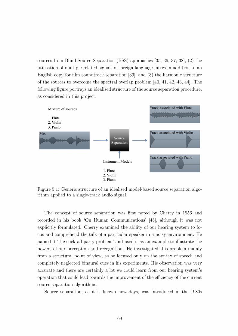
sources from Blind Source Separation (BSS) approaches [35, 36, 37, 38], (2) the

utilisation of multiple related signals of foreign language mixes in addition to an

English copy for film soundtrack separation [39], and (3) the harmonic structure

of the sources to overcome the spectral overlap problem [40, 41, 42, 43, 44]. The

following figure portrays an idealised structure of the source separation procedure,

as considered in this project.

Figure 5.1: Generic structure of an idealised model-based source separation algo-rithm applied to a single-track audio signal

The concept of source separation was first noted by Cherry in 1956 and

recorded in his book ‘On Human Communications’ [45], although it was not

explicitly formulated. Cherry examined the ability of our hearing system to fo-

cus and comprehend the talk of a particular speaker in a noisy environment. He

named it ‘the cocktail party problem’ and used it as an example to illustrate the

powers of our perception and recognition. He investigated this problem mainly

from a structural point of view, as he focused only on the syntax of speech and

completely neglected binaural cues in his experiments. His observation was very

accurate and there are certainly a lot we could learn from our hearing system’s

operation that could lead towards the improvement of the efficiency of the current

source separation algorithms.

Source separation, as it is known nowadays, was introduced in the 1980s

69

with the introduction of the first adaptive equalisers that were used in digital

communications [46, 47, 48, 49]. According to Comon et al. [50], the term

‘source separation’ was established only after 1987. A few other names were

used prior to it, such as source discrimination and source segmentation. The

first separation systems were dealing with instantaneous signals, which means

that the algorithms were memoryless. The objective was to cancel the effects of

a single-input, single-output (SISO) transmitting system to retrieve the original

signal at the terminal [50].

The technological advancement of the processing capabilities in combination

with the increase of the temporary and permanent storage space of today’s elec-

tronic equipment has enabled the processing of multiple-input, multiple-output

(MIMO) type of signals. Furthermore, it allows the development of sophisticated

source separation systems that can computationally afford the consideration of

several factors in order to achieve the separation of more complicated signals.

Today’s state of the art source separation algorithms manage the separation of

signals that contain more sources than the available mixtures that undergo pro-

cessing. Some examples are (1) Fitzgerald’s system that upmixes monophonic

recordings to stereophonic [51], (2) Audionamix’s algorithm that attempts to

separate the music and effects channels found in a soundtrack with the utilisa-

tion of additional copies of the soundtrack in different languages [39], and (3) a

commercial product that reduces/eliminates the spill of the adjacent drums in

the recording of the percussion of interest of a drum-kit [52].

5.2 Motivation, Aims and Objectives

Source separation algorithms are multi-dimensional systems that vary greatly

with respect to the methodology they follow and the nature of the data they

tackle. However, a generic model that can describe the vast majority is the

following:

• Transformation of the data to a representation where the structures of the

signal’s contents are well defined.

• Processing of the transformed data in order to distinguish and separate the

70

underlying sources.

• Transformation of the separated sources to the time domain to complete

the separation.

This project considers algorithms that apply processing in the frequency do-

main, and, more specifically, utilise the STFT for the transformation of the data.

Such algorithms attempt to distinguish and isolate the mixed sources by applying

processing to the spectral content of the signal. It is often, however, required to

further decrease the degree of complexity of the spectra of the signal prior to

the main processing in order to aid the algorithm distinguish between the “im-

portant” and the “unimportant” frequency components. This processing routine

is called spectral peak picking (see figure 5.2). The differentiation of the “im-

portant” from the “unimportant” frequency components is achieved with the

definition of a threshold. This technique is found in most of the projects that

focus on source separation in the University of York [53, 54, 55, 56, 57, 58, 59, 60].

It is, therefore, essential to investigate its performance and seek for optimisations,

where applicable.

Figure 5.2: An example of a thresholded spectrum from Benson’s work [53] (a)Original spectrum of mixture of cello and flute notes of different pitches. (b)Processed (data-reduced) spectrum of a) with the aid of a threshold. The unitsof the x and y axis are seconds and hertz, respectively

71

The estimation of this threshold may be achieved in numerous ways, some

of them being unintelligent and computationally inexpensive (static), and others

being sophisticated and computationally expensive (adaptive). The definition

of a static threshold is usually achieved through empirical observation of the

data by the developer and the utilisation of a simple model, such as linear or

exponential. This threshold is then assumed to be valid for every frame. Adaptive

thresholds are defined with regards to the contents of the subject frame, which

is achieved with the calculation of the spectral envelope and adjustment of its

parameters. An example of the function that achieves this is the moving average

filtering technique. Figure 5.3 portrays a set of static and adaptive examples of

thresholding.

The spectral peak picking technique has a number of weaknesses. Firstly,

setting a static threshold (1) results in the discard of the biggest part of the

amplitude spectrum, and hence the spectral coefficients, which can reduce the

credibility of processing techniques such as fundamental estimation (described in

5.3.2.4), and (2) may be particularly inefficient if the energy of the signal vary

with respect to time. Adaptive thresholding is not ideal either. The estimation

of the thresholding curve merely depends on the amplitude information of the

spectra, whose credibility and consistency varies greatly, as has been thoroughly

discussed in sub-section 2.3.1 on DFT and summarised in the introductory para-

graph of chapter 3. Moreover, there are many parameters that are user-specific

(window size, scaling etc.), which lead to yet another layer of complexity, whose

determination is made empirically.

These thresholding techniques are generic statistical tools that can be applied

to any data. On the other hand, phase stability, by definition, attempts to

differentiate the “structured” data from “noise” or edge effect/“artefacts”. Hence,

it is anticipated that the phase stability quality measure is more appropriate for

the reduction of the degree of complexity of the data, and thus can lead to

improved separation results.

The investigation of this hypothesis involves the development of a source sep-

aration algorithm that utilises the phase stability quality measure in the spectral

peak picking processing step. The aim here is to examine whether the phase

stability quality measure is effective. The idea is, instead of using any preset,

72

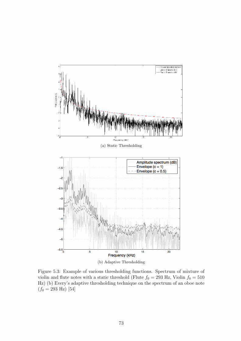
(a) Static Thresholding

(b) Adaptive Thresholding

Figure 5.3: Example of various thresholding functions. Spectrum of mixture ofviolin and flute notes with a static threshold (Flute f0 = 293 Hz, Violin f0 = 510Hz) (b) Every’s adaptive thresholding technique on the spectrum of an oboe note(f0 = 293 Hz) [54]

73

averaged or model threshold curve, to use a content-adaptive measure, which is

based entirely on phase information and consequently not dependent on the am-

plitude spectra and frame to frame variations in the amplitudes. The assessment

of the performance of the algorithm that incorporates the phase stability quality

measure will be achieved with its comparison to the performance of the same

algorithm that considers the unprocessed, conventional spectra.

5.3 The Algorithm

A numerical model-based source separation algorithm was programmed to test

the performance of the phase stability quality measure used as a threshold for

the reduction of the data of the conventional spectra. The algorithm, which is

instantiated twice, distinguishes the individual sources with the application of

a series of harmonic models on the (1) conventional amplitude spectra, and (2)

the data-reduced (with regards to phase stability) amplitude spectra. Then, the

fundamentals of the sources are estimated by processing the harmonic partials of

the selected models. Finally, the separation of the sources is achieved with the

application of spectral filters (binary masking), which are defined by the selected

harmonic models, on the original spectra obtained by the STFT algorithm and

transformation of the separated spectra in time domain.

The following sections describe the specification of the algorithm, document

its design, and examine the results for the assessment of the suitability of the

phase stability as a threshold measure in the data reduction step.

5.3.1 Specification

The specification of the source separation algorithm is directly related to the

nature of the signals that it attempts to separate. A set of restrictions were

imposed on the subject signals in order to make the goal attainable within the

time allocated for a masters programme.

Musical signals were considered with the following restrictions applied:

• Real instrument signals, excluding percussions and voice.

• Monophonic signals.

74

• A high Signal-to-Noise (SNR) ratio.

This is an important prerequisite due to the discrimination of the sources

with the aid of spectral models. It is therefore necessary for the partials

that exist due to the sources to be relatively greater in amplitude.

• Absence of artistic effects, such as reverb, distortion, delay etc.

Similarly, artistic effects are undesired because they introduce additional

partials that are not part of the instrument models or increase the noise

floor.

• Two instruments, approximately of the same amplitude with different fun-

damentals and not related in octave intervals, playing simultaneously.

• Consideration of the sustain part of the note.

• Stationarity.

• Harmonicity.

• A constrained range of possible note frequencies.

Further elaboration on the points with no comments of the previous bullet

list is included in the chapter regarding to further work 7.

5.3.2 Design

The algorithm is comprised of five main steps, which are included in the following

list. The description of each step is included in the following sub-sub sections.

1. Declaration of the parameters.

2. Import of the subject signals.

3. Analysis.

4. Voting system (fundamental estimation and generation of the spectral fil-

ters).

75

5. Separation and resynthesis.

Each of the above steps is a section of the main script, which serves as the

test-bench for the algorithm.

5.3.2.1 Declaration of the parameters

The declaration of the global settings of the entire algorithm is the first step

carried. The algorithm is completely parameterised, and every user-specific pa-

rameter is included in this section in order to make the testing of numerous cases

easier.

The parameters can be categorised in three main groups:

1. The STFT analysis parameters (frame size, overlap, zero padding factor,

windowing function, number of estimates for the ensemble approach (phase

stability mode), sample shift (phase stability mode)).

2. The mode of the algorithm (conventional or phase stability enhanced).

3. The parameters for the calculation of the harmonic models that are used for

the fundamental estimation and spectral filter generation in the voting stage

(the interval of frequencies where the fundamentals may lie, the number of

partials for each harmonic model, and the width of every partial).

5.3.2.2 Import of the subject signals

The sustain part of a violin and a flute note were selected in Cubase 7.5 from

the available recordings and mixed in a monophonic file, which is then imported

in the workspace of the algorithm. The subject signals used in this project are

courtesy of the Music Instrument Samples library produced by the University of

Iowa [34].

5.3.2.3 Analysis

Two analysis routines were programmed in order to obtain the necessary material

to assess the performance of the phase stability quality measure. Both routines

76

output two sets of data; (1) the complete set of spectra obtained from the con-

ventional STFT algorithm that is used in the separation and resynthesis stage,

and (2) an additional set of spectra, which differs for each routine, that is used

for the estimation of the fundamentals in the voting system.

The second set of data outputted from the first routine is the spectra obtained

from the conventional STFT algorithm with discarded mirrored coefficients. This

was necessary in order to reduce the computational expense of the algorithm.

The second set of data outputted from the second routine, which is also mirrored

coefficients-free, is the data-reduced (binary masked) spectra with regards to

the phase stability quality measure. The data reduction is a processing step

prior to the source separation that eliminates spectral components that are not

“structured”, according to the phase stability measure. Hence, they are assumed

to not be part of the sources. A threshold value was determined empirically

and kept the same for all frames. The flowcharts of the analysis routines are

depicted in figures 5.4 and 5.5. An example that illustrates the difference between

the unprocessed and processed amplitude spectra used in the voting system is

portrayed in figure 5.7, section 5.4. Additional comments on the differences are

provided.

5.3.2.4 Voting system

This step involves the generation of a set of harmonic models and their application

to the second set of data outputted by the analysis step in order to estimate the

fundamentals of the instruments and produce the appropriate spectral filters for

each source. This is achieved by correlating every individual model with the

data and, with some additional processing applied on the results, picking the

two models with the highest correlation degree for every frame. The partials of

the selected harmonic models are then processed for the determination of the

fundamentals for each frame, and the spectral filters are defined by allocating the

selected harmonic models in the corresponding variable.

The voting system section in the main script is comprised of three functions

that implement the aforementioned method; modelgen, modelpicker and specfilt.

Each function receives a combination of user-specific parameters and algorithm-

processed data. Their functionality is described in the following paragraphs.

77

Figure 5.4: Analysis routine 1 of the source separation algorithm: ConventionalSTFT Mode

78

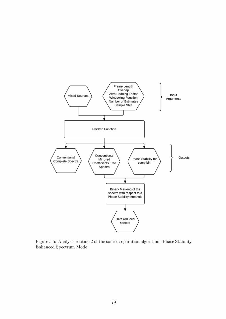
Figure 5.5: Analysis routine 2 of the source separation algorithm: Phase StabilityEnhanced Spectrum Mode

79

The modelgen function generates all possible harmonic models according to

the specification set by the user. The main arguments that determine the models

are the lowest possible fundamental (in Hz), the highest possible fundamental (in

Hz), the number of harmonics, and the width of every partial (in bins). Firstly,

the input arguments that describe the lowest and highest possible fundamental

frequencies in hertz are converted to the corresponding bins. Once this step has

been calculated, testing is applied in order to ensure that the highest partial,

which is comprised of the highest centre bin plus the additional bins specified

by the peakwidth argument, is within the limits of the analysed data (calculated

by the analysis step). The number of harmonic partials is adjusted accordingly,

if the highest harmonic partial exceeds the number of available bins. Then, the

harmonic partials of each model are calculated by dividing the highest possible

partial with the factor that describes the number of every lower partial. This

way the models describe all possible fundamental frequencies, even if it is undis-

tinguishable due to the fixed grid. The rest of the models are generated by

sequentially decreasing the centre bin of the highest harmonic partial by 1 bin,

until the centre bin of the lowest partial of the models reaches the limit set by the

user. Different weighting was applied for the first two harmonics, because of their

greater importance in the discrimination of the underlying sources. The first har-

monic peak contributes 3 times more and the second harmonic peak contributes

2 times more than the rest of the harmonic partials (see figure 5.6).

The modelpick function receives either the mirrored coefficient-free spectra or

the data reduced spectra and the generated models in order to determine the two

best fitting models for each frame, and calculate the fundamentals of the sources.

It calculates the correlation coefficient of each model with the subject frame by

multiplying the models with the amplitude spectrum element-wise and storing

the sum of the values of each product in a variable. Then, it selects the two

models with the highest correlation coefficient that meet the following criteria:

1. The model picked for the first instrument must not have a zero valued first

peak or great amplitude difference1 between the first and second peak.

2. The model picked for the second instrument must not (1) be an octave

1Empirically determined and set equal to 10.

80

Figure 5.6: Example of a harmonic model with 32 partials

above or below the model selected for instrument 1, and (2) have a zero

valued first peak or great amplitude difference1 between the first and second

peak.

Once these criteria are met, the index of the selected models for every frame

is stored in a variable and the fundamentals are calculated. This is achieved

by dividing every centre bin of each harmonic partial with the corresponding

partial number, and averaging the values. For instance, if bin 248 is the centre

bin of the 17th partial, the fundamental in hertz according to this estimate is24817×binresolution. The general expression for the estimation of the fundamental

is:

f0,v(m) =

∑Pp=1 centrebin(p)

p

P× binresolution (5.1)

Finally, the spectral filters for the separation of the sources for each frame are

compiled in specfilt. This function receives the indices of the selected models for

81

each instrument and frame, and the variable that holds the entire set of models. It

then creates two spectral filters, assigns the corresponding models, and calculates

the mirrored coefficients because they are applied to the original spectra obtained

by STFT. An additional spectral filter is generated for the residual components

that contains the bins that are not included either in the spectral filter of source

1 or 2. In the event of overlapping partials, the amplitude and the phase of

the frequency component are left intact. This may result in some augmented

frequency components in the instrument spectra, but it can be easily fixed with

simple filtering.

5.3.2.5 Separation and resynthesis

This step merely applies binary masking on the original spectra of the signal

with regards to the spectral filters obtained from the voting system. Finally, the

processed spectra (source 1, source 2 and residual) are transferred in time domain

with the utilisation of the istft function.

5.4 Result Review

The performance of the algorithm was judged successful by listening to the sep-

arated sources (available on the CD). The criteria for success was the lack of

sudden changes in pitch during the span of the note of the separated sources,

which could result from the incorrect selection of harmonic model for a particular

frame. Therefore, the separated sources had to resemble the pitch behaviour of

the original signals.

As was discussed in 5.3, the algorithm was instantiated twice, the only dif-

ference being the mode in which it ran and the number of partials comprising

the harmonic models. The number of the partials is of interest here because each

partial contributes an estimation of the fundamental for each source, in each

frame (see equation 5.1). Therefore, for a credible estimate of low variance, many

fundamental estimates are desired, and thus many partials. The rest of the pa-

rameters, which are included in table 5.1, remained the same for both instances

of the algorithm. Reasoning for the particular settings used is provided in the

following paragraphs.

82

The parameter of the analysis stage that required the most careful consid-

eration was the frame length. A window of 8192 samples long was found to be

appropriate, given the relative stationarity of the sources comprising the subject

signals used in this work. The application of a Hamming windowing function

was judged suitable for its accuracy in peak estimation (see table 2.1), which

also required the use of 50% overlap in order to achieve the resynthesis of the

separated sources without loss of energy. There was no need for frequency inter-

polation, since the length of the frame provided adequate frequency resolution.

The number of total estimates was set to 10, with a sample shift of 24, in the

case of phase stability mode.

Parameter Name ValueFrame length 8192

Overlap 4096Zero padding factor 0Windowing function HammingNumber of estimates 10

Sample shift 24

Table 5.1: Analysis parameters for both conventional and phase stability en-hanced modes

As was discussed in 5.3.2.3, the empirical definition of a threshold value with

regards to phase stability was required for the generation of the phase stability

enhanced spectra. The value of 0.009 was found appropriate, and kept constant

for all frames. Figure 5.7 illustrates the difference between the (1) conventional

amplitude spectrum and (2) the phase stability enhanced spectrum of the first

frame of the analysis for the aforementioned analysis parameters of the mixture

of signals as specified in 5.3.1. Moreover, an additional phase stability enhanced

spectrum is provided, which is produced with a different threshold value. This

graph is generated with a phase stability threshold value of 0.09 and is included

to showcase the difference in which it results.

Regarding to the voting system parameters, the interval of potential funda-

mental frequencies specified by the user was 130 - 670 Hz, which covers two

western musical octaves. This was found to be a satisfactory starting point, since

big part of the mainstream lead melodies lie within the aforementioned limits.

83

Figure 5.7: Analysis of a mixture of violin and flute notes. (a) Conventional am-plitude spectrum (b) Phase Stability Enhanced Spectrum (PSES) with thresholdvalue 0.009 (c) Phase Stability Enhanced Spectrum (PSES) with threshold value0.09

84

The width of every partial peak was set to 5 bins in order to abide by the prop-

erties of the main lobe of the Hamming window function (see table 2.1). Finally,

the number of harmonic partials varied for each mode. It was found that the

algorithm in conventional mode meets the performance criteria only with mod-

els that contain up to 23 harmonic partials, whereas in phase stability enhanced

mode can use 32 harmonic partials (maximum number that the models can fit

due to the available number of bins and the interval of potential fundamentals).

To conclude, the capability of the phase stability enhanced algorithm to sepa-

rate sources with the application of harmonic models of a larger number of partials

than the conventional instance proves that the phase stability quality measure

is appropriate for the efficient reduction of the complexity of the data. Having

eliminated the “unstable” frequency components (bins) results into an amplitude

spectrum that theoretically contains only the “important” components and no

baseline “noise”. This improves the performance of the step that correlates the

harmonic models with the analysed data, as there are less “unstable” bins to con-

tribute into the calculation of the correlation coefficient. Finally, it also improves

the performance of the algorithm in two ways:

1. the estimation of the fundamentals is more accurate, credible and of smaller

variations, since more partials contribute in the estimation of the fundamen-

tal frequency for every source, in every frame,

2. and the separated sources contain a higher number of harmonics, which

results in separated results of higher quality.

85

Chapter 6

Conclusions

One of the most important, yet least considered, assumptions of the STFT was

investigated in this work, stationarity. This principle that forms the foundation

of the STFT and also happens to be one of its greatest deficiencies often results

in potentially misleading data. A novel method was proposed and examined

that attempts to circumvent this limitation of STFT. This method attempts

to achieve comprehensible results of greater credibility with the allowance of a

certain degree of deviation from stationarity incorporated into the analysis. This

was achieved by constructing an ensemble of closely-related spectral estimates

instead of a single estimation in order to acquire the short-time phase evolution

of each frequency bin. The phase information is then compared to that of a

model of an idealised but not necessarily stationary partial of an acoustic source

in order to define a quality measure that discriminates the “structured” from

the “unstructured” frequency bins. This quality measure, named phase stability,

describes the degree of deviation of the phase behaviour of a subject frequency

bin from the behaviour of its corresponding idealistic frequency component. The

incorporation of a certain degree of deviation from stationarity is achieved with

the consideration of non-stationary idealistic frequency components. The results

of the phase stability of the sustain portion of real signals exhibited a flatter

frequency response in contrary to the common high-frequency roll off that is

found in the amplitude spectra and had greater dynamic range than the amplitude

spectra.

The potential of this quality measure was then investigated with its incor-

86

poration in the framework of source separation, as a single application example.

Used in the spectral peak picking step of a numerical model-based algorithm,

it was found that it effectively reduces the complexity of the spectra of a mix-

ture of signals without the discard of the “important” frequency components.

The assessment of the effectiveness of the processed spectra was achieved with

their consideration in the separation step, where numerous harmonic models were

applied to them in order to distinguish the underlying sources. The algorithm

successfully separated the mixture of the sustain parts of the two notes, flute

and violin, with the utilisation of harmonic models that contain a larger number

of partials than the instance of the algorithm that considered the conventional

amplitude spectra (in this simple exemplar case, success was judged entirely by

ear as opposed to using quantitative measures). This resulted in better informed

estimates of fundamental frequency, since more harmonic peak position estimates

are available.

The results obtained from the application of the phase stability in the frame-

work of source separation are promising. It is anticipated that this quality mea-

sure has great potential, in particular where there can be assumed relative phase

continuity. The aim of this project was to set the fundamental principles and

groundwork, which was successfully accomplished. However, there are multiple

aspects that were not examined due to the lack of time. A set of aims is de-

fined in the following chapter regarding further work in order to prompt further

investigation and development of the proposed method.

87

Chapter 7

Further Work

The complete and thorough investigation of the subject topics of this project was

impossible within the limited amount of time allocated for an one-year research

project. Careful consideration was given to select the vital aspects that required

investigation in order to obtain an essential insight to the problem, establish the

foundation and prompt further work, accordingly.

This chapter consolidates a framework that includes the additional aspects

that require investigation and further exploration. The two main topics on which

this project elaborates are phase stability and source separation. Hence, the

suggested further work is documented as such.

7.1 Phase Stability

The investigation of the behaviour of the phase stability quality measure of addi-

tional signals of greater variety is required. This project focused on the analysis

of musical signals, initially synthetic and then real, and, in particular, it consid-

ered the sustain part of harmonic instrument signals. This type of signals was

considered in order to introduce the notion of ‘stability’ in phase information.

However, phase stability is anticipated to yield interesting insights in all types of

musical signals (and not only!). Specifically, it is speculated that it can provide

interesting results in the analysis of transients (i.e. percussive sounds), where

there are “structured” components (i.e. the pitch in which the drum is tuned,

which results to a fundamental frequency component), as well as “unstructured”

(i.e. the attack phase of the percussive sound). It is likely that this measure can

88

be used as an indicator for the beginning and ending points of attack and sustain

phases. Moreover, this concept is expected to be applicable to any type of signals

that exhibit phase continuity.

The implementation of the proposed method that obtains the phase stability

quality measure resulted in two additional user-specific parameters; number of

additional estimates (Q) and sample shift (C). These variables have an impor-

tant impact on the analysed results. Large number of estimates, Q, may result

into more accurate phase behaviour modelling, but that might not be an option

depending on the frame length and hop size set in the STFT. Ideally, the rela-

tively short-term phase behaviour is of interest, and the total amount of sample

shift due to the additional estimates is desired to be relatively small with regards

to the predifined frame lenght of the analysis, because otherwise the analysis

could be associated with an analysis of very high temporal interpolation.

The aforementioned concerns have important impacts in speech and thus for-

mant analysis. Despite the fact that phase stability is expected to be appropriate

for the analysis of speech signals due to their structured spectral behaviour, it

might not be possible due to the very short frame lengths with which speech is

usually analysed (i.e. frames of 256 samples). The construction of an ensemble of

10 estimates with a shift of 4 samples in between, results in a total of 40 samples,

which corresponds to 15% of a frame length of 256 samples. Nevertheless, it is

definitely worthy of investigation, since even a sample shift of 2 could potentially

yield interesting results.

This method may also have uses of a different fashion. The allowance of a cer-

tain degree of deviation from stationarity within the analysis, which is achieved

with the comparision of the analysed data with the modelled short-time phase be-

haviour of non-stationary frequency components, is implemented with the fitting

of a quadratic curve to the data of the form:

at2 + bt+ c (7.1)

where a, b, and c are the calculated coefficients.

For stationary signals, a is approximately zero. However, for non-stationary

89

signals, a corresponds to the degree of linear change in phase, and hence frequency.

Therefore, it could be exploited for chirp rate estimation purposes.

Finally, the incorporation of the phase stability in additional areas and ap-

plications requires careful consideration. An example is provided in this project

with the incorporation of the phase stability in a numerical model-based source

separation algorithm, and it is shown that its potential is great.

7.2 Source Separation

The specification of the source separation algorithm have been introduced in 5.3.1

with the definition of the type of signals that it is able to separate. This restricted

sub-group of musical signals was selected as a starting point in order to obtain a

better insight into the problem of separation and establish the necessary ground-

work. The envisioned improved version of the project’s algorithm is expected

to be more versatile and capable. The aim is to develop it further in order to

enable it to process the standard type of musical signals that are common nowa-

days. The restrictions, as stated by the bullet points, that can be overcome are

included in the following paragraphs, along with the proposed work.

• Real instrument signals, excluding percussions and voice.

Expanding the algorithm’s capabilities to enable it to consider voice should

be relatively simple, since modelling formants in the frequency domain is

achievable. However, the consideration of percussions would be more chal-

lenging due to the unstructured behaviour of their spectral information.

Nevertheless, an interesting approach has been suggested for the separation

of percussive sounds from the rest of the mixture of instrumental signals in

the frequency domain by Fitzgerald [51], which is anticipated to be appro-

priate for incorporation in the current algorithm.

• Monophonic signals.

The consideration of stereophonic signals is anticipated not only to be pos-

sible but also to provide additional exploitable information (directionality)

that will help in the separation of the sources. Moreover, the phase stability

90

quality measure might be another measure for consideration in addition to

amplitude. Similar phase stability values with a certain delay between the

two channels is expected to aid in the discrimination of the sources.

• Two instruments, approximately of the same amplitude with different fun-

damentals and not related in octave intervals, playing simultaneously.

There has been done work on the discrimination of instrument notes that

are related in octave intervals in [57], and the incorporation of the proposed

method in the current algorithm is expected to be feasible. However, the

consideration of instrument notes of the same pitch is expected to be much

more challenging, since there is a great amount of overlap in pitch between

different instruments in today’s western music. Nevertheless, it is definitely

an area that requires attention.

• Consideration of the sustain part of the note.

The attack phase of a note is not considered because its modelling in fre-

quency domain is rather complicated. Nonetheless, preliminary work of a

different fashion that attempts to identify the non-allocated attack parts

found in the residual component source and assign them to the correspond-

ing source has been done in [60]. This is achieved by obtaining the ‘fin-

gerprint’ of the attack phases identified in the residual source and trying

to match it with the separated source to which it belongs. This approach

can be further investigated and developed in order to incorporate it in the

current algorithm and enable it consider whole notes.

• Stationarity.

The assumption of stationarity is implied in general in the use of Fourier

approaches and, of course, is in general not true. Part of the purpose of

this work is the development of a method that allows a certain degree of

deviation from stationarity to be incorporated into the analysis process, as

represented by the curvature of the phase evolution curve.

• Harmonicity.

91

Likewise, harmonicity is a widely used assumption and although exploited

here, for simplicity, more realistic spectral models can be used, as imple-

mented in [56].

• A constrained range of possible note frequencies.

This step requires additional investigation, since it has been noticed that

for the current settings of this project, the performance of the algorithm

varies (in terms of the number of harmonic partials with which successful

separation is achieved) with respect to the subject signals.

Finally, the energy allocation of overlapping partials is an issue that requires

attention. The current algorithm merely allocates the full amount of energy to

both sources. However, this results in the introduction of additional energy. It

is therefore required to implement a method that measures the relative energy of

each source for every frame in order to allocate the respective amount of energy

of the overlapping partial to each source accordingly. This way the preservation

of energy can be achieved. Moreover, the coherent reconstruction of the phase

of each modified bin is required. The modification of the amplitude information

of a bin during the energy allocation of overlapping partials may result in the

reconstruction of perceptually bad sounding sources. This issue is discussed in

Le Roux’s et al. [61] and Fitzgerald’s paper on masking filters [62] where methods

for tackling it are suggested.

92

Appendix A: Initial phase anglesobtained from the analysis of thecosine in chapter 3


(rads)


(rads)


(rads)


(rads)Bin 1 3.142 3.142 3.142 3.142Bin 2 1.647 2.85 -3.065 -2.697Bin 3 1.724 2.635 -2.988 -2.328Bin 4 -1.341 -0.636 0.23 1.096Bin 5 -1.264 -0.703 0.306 1.316Bin 6 -1.188 -0.729 0.383 1.495Bin 7 -1.111 -0.729 0.46 1.649Bin 8 -1.034 -0.712 0.536 1.784Bin 9 -0.958 -0.682 0.613 1.908Bin 10 -0.881 -0.645 0.69 2.024Bin 11 -0.805 -0.601 0.766 2.133Bin 12 -0.728 -0.552 0.843 2.238Bin 13 -0.651 -0.501 0.919 2.34Bin 14 -0.575 -0.447 0.996 2.439Bin 15 -0.498 -0.39 1.073 2.536Bin 16 -0.421 -0.332 1.149 2.631Bin 17 -0.345 -0.273 1.226 2.725Bin 18 -0.268 -0.214 1.303 2.819Bin 19 -0.192 -0.153 1.379 2.911Bin 20 -0.115 -0.092 1.456 3.004Bin 21 -0.038 -0.031 1.532 3.096

93

Appendix B: Initial phase anglesobtained from the analysis of thecosine with vibrato in chapter 3


(rads)


(rads)


(rads)


(rads)Bin 1 3.142 3.142 3.142 0Bin 2 2.235 3.088 -2.814 0.032Bin 3 2.62 -3.001 -2.35 -1.488Bin 4 -0.657 0.195 1.063 1.759Bin 5 -0.874 0.198 1.321 2.142Bin 6 -0.864 0.257 1.501 2.115Bin 7 -0.783 0.337 1.632 2.072Bin 8 -0.75 0.395 1.765 2.134Bin 9 -0.717 0.443 1.892 2.208Bin 10 -0.676 0.49 2.01 2.282Bin 11 -0.628 0.533 2.122 2.355Bin 12 -0.576 0.572 2.228 2.429Bin 13 -0.521 0.605 2.331 2.504Bin 14 -0.464 0.63 2.431 2.578Bin 15 -0.405 0.645 2.53 2.653Bin 16 -0.345 0.643 2.626 2.728Bin 17 -0.283 0.621 2.721 2.803Bin 18 -0.221 0.567 2.816 2.878Bin 19 -0.158 0.471 2.909 2.953Bin 20 -0.095 0.32 3.002 3.029Bin 21 -0.032 0.115 3.095 3.104

94

Appendix C: Initial phase anglesobtained from the analysis of thecosine with glissando in chapter 3


(rads)


(rads)


(rads)


(rads)Bin 1 3.142 0 0 0Bin 2 -2.926 -1.316 -0.07 0.267Bin 3 -2.763 -1.464 -0.193 0.449Bin 4 -2.974 -1.895 -0.668 0.232Bin 5 0.451 1.553 2.643 -2.42Bin 6 1.147 2.11 -3.041 -1.638Bin 7 1.355 2.171 -3.047 -1.487Bin 8 1.517 2.22 -3.077 -1.368Bin 9 1.666 2.276 -3.098 -1.253Bin 10 1.806 2.337 -3.114 -1.14Bin 11 1.939 2.402 -3.126 -1.031Bin 12 2.067 2.469 -3.134 -0.925Bin 13 2.19 2.537 -3.14 -0.822Bin 14 2.309 2.606 3.139 -0.721Bin 15 2.425 2.676 3.136 -0.622Bin 16 2.539 2.747 3.135 -0.524Bin 17 2.651 2.818 3.135 -0.427Bin 18 2.761 2.89 3.135 -0.331Bin 19 2.871 2.962 3.137 -0.236Bin 20 2.979 3.034 3.139 -0.142Bin 21 3.088 3.106 3.141 -0.047

95

Appendix D: Application ofartificial vibrato on the violinsample in Cubase 7.5

96

Appendix E: Application ofartificial glissando on the violinsample in Cubase 7.5

97

Appendix F: The stft function

1 function [ X ] = stft( ...x,frame,overlap,zpf,window,nEnsemble,sampleshift )

2 %STFT Short-Time Fourier Transform3 % [X]=STFT(X,FRAME,OVERLAP,ZPF,WINDOW) returns the ...

Short-Time Fourier4 % Transform of the vector x in the matrix X. Three window ...

functions are5 % available; rectangular, Hamming and Hanning. ...

[X<NFRAMES:NFFT>]6 %7 % ...

[X]=STFT(X,FRAME,OVERLAP,ZPF,WINDOW,NENSEMBLE,SAMPLESHIFT) ...implements

8 % the ensemble of closely-related estimates approach. It ...calculates

9 % (NENSEMBLE-1) additional spectra for each frame ...determined by the

10 % conventional STFT algorithm. An offset equal to ...SAMPLESHIFT is

11 % introduced to each additional estimate. ...[X<NENSEMBLE:NFFT:NFRAMES>]

12 %13 % This function can receive either monophonic or ...

stereophonic signals. If14 % the input signal is sterephonic, it converts it to ...

monophonic.15 %16 %Example:17 % x = sin(2*pi*(800/44100)*(0:44099));18 % X1 = stft(x,4096,0,0,'rectwin'); % Conventional STFT.19 % X2 = stft(x,4096,0,0,'rectwin',10,24); % Ensemble STFT ...

for PSES.20 %21 %Author:22 % Thomas Arvanitidis, thomasarvanitidis AT gmail DOT com23 %

98

24 %History:25 % 05/01/2014: Programmed and Documented.26 % 03/03/2014: Implemented ensemble of estimations approach ...

(PASS w EASE).27 % 30/06/2014: Thorough testing, bug fix and optimisation.28 % 08/07/2014: Corrected the zero-padding logic for the PASS ...

with EASE29 % functionality.30 % 10/07/2014: Modified to store the ensemble FT into a 3 ...

dimensional31 % matrix instead of a cell array.32 % 01/10/2014: Produced the generic formula for the ...

calculation of33 % nframes, which works for both conventional ...

and ensemble34 % approach.35 % 02/10/2014: Corrected the expression for the calculation ...

of the number36 % of frames. From ...

(L-(nEnsemble-1)*sampleshift-hop)/(hop)37 % to (L-(nEnsemble-1)*sampleshift-overlap)/(hop).38

39 % Argument check.40 if nargin < 6, nEnsemble = 1; end41 if nargin < 7, sampleshift = 0; end42 assert(all(isscalar(frame)==1&&isscalar(overlap)==1&&...43 isscalar(zpf)==1&&isscalar(nEnsemble)==1&&...44 isscalar(sampleshift)==1), ...45 'Ensure frame,overlap,zpf,nEnsemble and sampleshift are ...

scalars.')46 assert(all(ischar(window)),'Window should be char variable')47 assert(all(isvector(x)==1) | |(size(x,1)==2 | |size(x,2)==2),...48 'Subject signal must be either monophonic or stereo') % ...

Assert x is either monophonic or stereo.49 if size(x,1)==2 | | size(x,2)==250 if size(x,2)==2, x = x'; end % ...

If x is stereo51 x = 0.5.*(x(1,:) + x(2,:)); % ...

convert x to monophonic.52 end53 if iscolumn(x) == 1, x = x'; end % ...

Represent x as row-vector if it is not.54

55 % Generate window function.56 switch window % Window functions are (all =0 outside the ...

interval 0≤n≤wl)57 case 'rectwin'58 win=ones(1,frame); % Rectangular Window59 case 'hann'

99

60 win=hann(frame,'periodic')'; % Hann window ...w[n]=0.5-0.5*cos(2*pi*n/M), for 0≤n≤M

61 % win=hann2(frame)'; % Hann window ...w[n]=0.5-0.5*cos(2*pi*n/M), for 0≤n≤M

62 case 'hamming'63 win=hamming(frame,'periodic')'; % Hamming window ...

w[n]=0.54-.46*cos(2*pi*n/M) for 0≤n≤M64 % win=hamming2(frame)'; % Hamming ...

window w[n]=0.54-.46*cos(2*pi*n/M) for 0≤n≤M65 otherwise66 win=ones(1,frame);67 disp('Invalid window type, defaulting to rectangular ...

window.');68 end69

70 % General parameters.71 L = length(x);72 hop = frame - overlap;73 if zpf 6= 0, nfft = (zpf+1)*frame; else nfft = frame; end74 nframes = floor((L-(nEnsemble-1)*sampleshift-overlap)/(hop));75

76 % Instantiate FT variable.77 if nEnsemble == 1 % Conventional STFT variables.78 X = zeros(nframes,nfft);79 else % PASS with EASE variables.80 X = zeros(nEnsemble,nfft,nframes);81 end82

83 % Calculate window normalisation factor.84 if strcmp(window,'rectwin') && overlap == 085 wnorm = sum(win)/frame;86 elseif (strcmp(window,'hann') | | strcmp(window,'hamming')) && ...

overlap == frame/287 wnorm = 2.*sum(win)/frame;88 % else89 % error('myApp:argChk', 'Wrong combination of input ...

arguments, window and overlap.')90 end91 wnorm = 2.*sum(win)/frame;92 % Main function.93 str = 1; len = frame;94 if nEnsemble == 195 % Conventional STFT.96 for i = 1:nframes97 temp = x(str:len).*win/wnorm; % Frame picking ...

and normalised windowing. This (sum(win)/nfft) ...used to be (4.*sum(win)/nfft) but gave wrong ...results during the resynthesis stage.

98 X(i,:) = fft(temp,nfft); % Analysis.

100

99 str=str+hop; len=str+frame-1; % Index variables ...update.

100 end101 else102 % PASS with EASE.103 for i = 1:nframes104 for obs = 1:nEnsemble % Each ...

observation is a FT analysis.105 % Frame picking and normalised windowing.106 temp = x((obs-1)*sampleshift+str:...107 (obs-1)*sampleshift+len).*win/wnorm;108 X(obs,:,i) = fft(temp,nfft); % Analysis.109 end110 str=str+hop; len=str+frame-1; % Index variables ...

update.111 end112 end

101

Appendix G: The phistabfunction

1 function [ output,mode ] = ...phistab(data,frame,overlap,zpf,window,nEnsemble,...

2 sampleshift,det,order)3 %PHISTAB Phase Stability4 % ...

[OUTPUT]=PHISTAB(X,FRAMELENGTH,OVERLAP,ZPF,WINDOW,NENSEMBLE,...5 % SAMPLESHIFT,DET,ORDER) calculates the phase stability ...

quality ...6 % measure for the analysed data.7 %8 %Notes:9 % This function is dependent on the modified STFT function ...

developed by10 % Thomas Arvanitidis.11 %12 %Example:13 % x = sin(2*pi*(80/44100)*(0:44099));14 % [data,¬] = phistab(x,4096,0,0,'rectwin',10,24);15 %16 %Author:17 % Thomas Arvanitidis, thomasarvanitidis AT gmail DOT com18 %19 %History:20 % 26/04/2014: Programmed and documented.21 % 09/07/2014: Substituted detrend with polyfit/polyval.22 % 29/07/2014: Added progress feedback.23 % 29/09/2014: Renamed the function from IPV to PSES.24 % 16/10/2014: Renamed the function from PSES to PHISTAB.25

26 % Argument check.27 if nargin < 8, det = 0; end % Preset det to 0 to disable ...

functionality.

102

28 if nargin < 9, order = 2; end % Order of polynomial fit by ...polyfit.

29 assert(all(isscalar(frame)==1&&isscalar(overlap)==1&&...30 isscalar(zpf)==1&&isscalar(nEnsemble)==1&&...31 isscalar(sampleshift)==1&&isscalar(det)==1&&...32 isscalar(order)==1),'Ensure frame,overlap,zpf,nEnsemble ...

and sampleshift are scalars.')33 assert(all(ischar(window)),'Window should be char variable')34 assert(all((nEnsemble>1)),'nEnsemble must be bigger than 1')35 assert(all((sampleshift>0)),'sampleShift must be bigger than 0')36 assert(all((det==1 | |det==0)),'Det can either be on (1) or off ...

(0)')37 assert(all((order>0&&order<3)),'Polynomial can either be of ...

1st or 2nd order')38

39

40 % Data calculation.41 DATA = stft(data,frame,overlap,zpf,window,nEnsemble,sampleshift);42 DATA = DATA(:,1:size(DATA,2)/2+1,:); % Discard mirrored ...

coefficients.43

44 % Parameter setting.45 nObs = size(DATA,1); % # of ensemble.46 nBins = size(DATA,2); % # of bins.47 nFrames = size(DATA,3); % # of frames.48

49 % Variable declaration: Polyfit/Polyval.50 idx = (1:nObs)'; % Polyval input indices.51 r = zeros(nObs,nBins,nFrames); % Phase variance.52 r2 = zeros(nFrames,nBins); % Sum of least ...

squares (Phase Stability).53 r2i = zeros(nFrames,nBins); % Inverse Phase Variance.54 angles = zeros(nObs,nBins,nFrames); % STFT unwrapped angles.55 coef = zeros(order+1,nBins,nFrames); % Polyfit coefficients.56 modelang = zeros(nObs,nBins,nFrames); % Polyval output ...

values (modelled angles).57

58 % The followings are available for comparison purposes (det ...vs. polyfit/val).

59 % This comparison can only be made if the order of the ...polyfit is set to 1.

60 % Variable declaration: Detrend.61 if det == 1 % Instantiate only if ...

requested.62 rdet = zeros(nObs,nBins,nFrames); % Phase variance.63 r2det = zeros(nFrames,nBins); % Sum of least ...

squares (Phase Stability).64 r2idet = zeros(nFrames,nBins); % Inverse Phase Variance.65 end

103

66

67 % Monitoring the progress of the function.68 ur = 0.2; % Update rate 20%.69 step = nFrames*ur; % Step interval.70 nsteps = 1:(1/ur); % Number of steps.71 updatesteps = step.*nsteps; % Feedback display indeces.72 updatesteps = ceil(updatesteps); % Rounded-up indeces.73 countPrint = 1; % Feedback algorithm flag.74

75 % Main: Phase stability algorithm.76 for i = 1:nFrames77 angles(:,:,i) = unwrap(angle(DATA(:,:,i))); % Unwrap ...

the angles.78 for ii = 1:nBins79 coef(:,ii,i) = polyfit(idx,angles(:,ii,i),order); % ...

Calculate the curve coefficients for each bin.80 modelang(:,ii,i) = polyval(coef(:,ii,i),idx); % ...

Calculate the modelled angles.81 r(:,ii,i) = angles(:,ii,i)' - modelang(:,ii,i)'; % ...

Phase variance.82 end83 r2(i,:) = sum(r(:,:,i).*r(:,:,i)); % Sum of ...

least squares of phase variance (Phase Stability).84 r2i(i,:) = 1./(r2(i,:)+eps); % Inverse ...

Phase Variance <nFrames x nBins>85

86 % The followings are available for comparison purposes ...(det vs. polyfit/val).

87 % Curve fitting with DETREND.88 if det == 189 rdet(:,:,i) = detrend(angles(:,:,i)); % ...

Phase variance.90 r2det(i,:) = sum(rdet(:,:,i).*rdet(:,:,i)); % Sum ...

of least squares of phase variance (Phase Stability).91 r2idet(i,:) = 1./(r2det(i,:)+eps); % ...

Inverse Phase Variance <nFrames x nBins>92 end93

94 % Progress feedback.95 if any(i==updatesteps) % Display percentage on ...

specific steps.96 done = (i*100)/nFrames; % Calculate percentage completed.97 if countPrint == 1, fprintf('PS analysis percentage: ...

%.1f\n',done);98 else fprintf('\b\b\b\b\b%.1f\n',done); end99 countPrint = countPrint +1;

100 end101 end102

104

103 % Select return variables.104 switch nargout105 case 1106 output = r2i; % Inverse Phase ...

Variance <nFrames x nBins>107 otherwise108 output.IPV = r2i; % Inverse Phase ...

Variance <nFrames x nBins>109 output.r = r; % Phase variance.110 output.PS = r2; % Least squares of ...

phase variance (Phase Stability).111 output.angles = angles; % Unwrapped angles ...

{nFrames,1}(nObs x nBins)112 output.modelang = modelang; % Modelled angles ...

{nFrames,1}(nObs x nBins)113 output.coef = coef; % Polynomial ...

coefficients {nFrames,1}(3 x nBins). 3 due to 2nd ...order polyfit.

114 mode = 'monitoring'; % Dummy variable.115 if det == 1116 output.IPVdet = r2idet; % DETREND Inverse ...

Phase Variance <nFrames x nBins>117 output.rdet = rdet; % DETREND Phase variance.118 output.PS = r2det; % DETREND Least ...

squares of phase variance (Phase Stability).119 end120 end

105

Nomenclature

Roman Symbols

A Amplitude

C Sample shift

E Energy

f Frequency

fs Sampling Frequency

H Step size

I Imaginary

L Frame Length

M Number of Frames

N Signal length

n Time (discrete)

P Number of Partials

Q Number of spectral estimates

R Real

s Fourier basis

t Time (continuous)

106

X Fourier transform of signal x

x Signal

Greek Symbols

ω Angular frequency

φ(0) Initial phase angle

π ' 3.14 . . .

ϕ Phase angle

Superscripts

j unit imaginary number√−1

Subscripts

d Harmonic partial index

k Frequency counter

m Frame counter

p Partial index

v Source index

Acronyms

ADSR Attack-Decay-Sustain-Release

ASTFT Adaptive Short-Time Fourier Transform

BSS Blind Source Separation

CIF Channelised Instantaneous Frequency

DFT Discrete Fourier Transform

DSP Digital Signal Processing

107

FFT Fast Fourier Transform

IDFT Inverse Discrete Fourier Transform

IFFT Inverse Fast Fourier Transform

ISTFT Inverse Short-Time Fourier Transform

LGD Local Group Delay

MIMO Multiple-input, multiple-output

nfft Number of points considered by FFT

PSD Power Spectral Density

PSES Phase Stability Enhanced Spectra

SISO Single-input, single-output

SNR Signal-to-Noise ratio

STFT Short-Time Fourier Transform

TCIF Time-Corrected Instantaneous Frequency

zpf Zero padding factor

108

References

[1] G. Pokol, L. Horvath, N. Lazanyi, G. Papp, G. Por, and V. Igochine, “Con-

tinuous linear time-frequency transforms in the analysis of fusion plasma

transients,” in 40th EPS Conf. on Plasma Physics, Espoo, Jul. 1-5, 2013,

pp. 1306–1309.

[2] R. Thirumalainambi and D. E. Thompson, “Gravitational Wave Signal iden-

tification and transformations in time-frequency domain,” NASA, Tech.

Rep.

[3] K. Darowicki and W. Felisiak, “On the joint time-frequency characteristics

of chemical oscillations,” J. of Computational Chemistry, vol. 27, no. 8, pp.

961–965, 2006.

[4] D. Tuncel, A. Dizibuyuk, and M. Kiymik, “Time Frequency Based Coherence

Analysis Between EEG and EMG Activities in Fatigue Duration,” J. of

Medical Syst., vol. 34, no. 2, pp. 131–138, 2010.

[5] Z. N. E. and H. R. Siahkoohi, “Single Frequency Seismic Attribute Based

on Short Time Fourier Transform, Continuous Wavelet Transform, and S

Transform,” in 6th Conf. & Exposition on Petroleum Geophysics, Kolkata,

Jan. 2006.

[6] T. Pinch and F. Trocco, Analog days : the invention and impact of the Moog

synthesizer. Cambridge, MA: Harvard University Press, 2002.

[7] Wikipedia. Arp odyssey. Accessed: 2014-12-17. [Online]. Available:

http://en.wikipedia.org/wiki/ARP Odyssey

109

http://en.wikipedia.org/wiki/ARP_Odyssey

[8] J. Moorer, “Signal processing aspects of computer music: A survey,” in Proc.

of the IEEE, vol. 65, no. 8, Aug. 1977, pp. 1108–1137.

[9] D. M. Howard and J. S. Angus, Acoustics and psychoacoustics, 4th ed. Ox-

ford: Focal, 2009.

[10] L. V. Barbosa, “Fourier Transform Time and Fre-

quency domains,” accessed: 2014-12-17. [Online]. Avail-

able: http://en.wikipedia.org/wiki/Fourier transform#mediaviewer/File:

Fourier transform time and frequency domains (small).gif

[11] J. O. Smith. Spectral Audio Signal Processing. Accessed: 2014-12-17.

[Online]. Available: http://www.dsprelated.com/dspbooks/sasp/

[12] J. W. Cooley and J. W. Tukey, “An Algorithm for the Machine Calculation

of Complex Fourier Series,” Math. of Computation, vol. 19, no. 90, pp. 297–

301, Apr. 1965.

[13] F. J. Harris, “On the use of windows for harmonic analysis with the discrete

Fourier transform,” Proc. of the IEEE, vol. 66, no. 1, pp. 51–83, Jan. 1978.

[14] A. H. Nuttall, “Some windows with very good sidelobe behavior,” IEEE

Trans. Acoust., Speech, Signal Process., vol. 29, no. 1, pp. 84–91, Feb. 1981.

[15] J. B. Allen, “Short term spectral analysis, synthesis, and modification by

discrete fourier transform,” IEEE Trans. Acoust., Speech, Signal Process.,

vol. 25, no. 3, pp. 235–238, Jun. 1977.

[16] M. S. Bartlett, “Smoothing Periodograms from Time-Series with Continuous

Spectra,” Nature, vol. 161, pp. 686–687, May 1948.

[17] ——, “Periodogram Analysis and Continuous Spectra,” Biometrika, vol. 37,

no. 1/2, pp. 1–16, Jun. 1950.

[18] P. D. Welch, “The use of fast Fourier transform for the estimation of power

spectra: A method based on time averaging over short, modified peri-

odograms,” IEEE Trans. Audio Electroacoust., vol. 15, no. 2, pp. 70–73,

Jun. 1967.

110

http://en.wikipedia.org/wiki/Fourier_transform#mediaviewer/File:Fourier_transform_time_and_frequency_domains_(small).gif

http://en.wikipedia.org/wiki/Fourier_transform#mediaviewer/File:Fourier_transform_time_and_frequency_domains_(small).gif

http://www.dsprelated.com/dspbooks/sasp/

[19] P. Depalle and T. Helie, “Extraction of spectral peak parameters using a

short-time Fourier transform modeling and no sidelobe windows,” in IEEE

ASSP Workshop on Applications of Signal Processing to Audio and Acous-

tics, Oct. 1997, p. 4.

[20] A. Oppenheim, D. Johnson, and K. Steiglitz, “Computation of spectra with

unequal resolution using the fast Fourier transform,” in Proc. of the IEEE,

vol. 59, no. 2, Feb. 1971, pp. 299–301.

[21] J. C. Brown, “Calculation of a constant Q spectral transform,” The J. of the

Acoustical Soc. of America, vol. 89, no. 1, pp. 425–434, 1991.

[22] A. Lukin, “Multiresolution STFT for Analysis and Processing of Audio,”

Talk at B.U., September 2010. [Online]. Available: audio.rightmark.org/

lukin/temp/exchange/LukinTalk.ppt

[23] D. L. Jones and T. W. Parks, “A high resolution data-adaptive time-

frequency representation,” in IEEE Trans. Acoust., Speech, Signal Process.,

vol. 38, no. 12, pp. 2127–2135, Dec. 1990.

[24] D. Rudoy, P. Basu, T. Quatieri, B. Dunn, and P. Wolfe, “Adaptive short-time

analysis-synthesis for speech enhancement,” in IEEE Int. Conf. on Acoustics,

Speech, and Signal Processing (ICASSP 2008), Mar. 2008, pp. 4905–4908.

[25] S. A. Fulop and K. Fitz, “Algorithms for computing the time-corrected in-

stantaneous frequency (reassigned) spectrogram, with applications,” The J.

of the Acoustical Soc. of America, vol. 119, no. 1, pp. 360–371, 2006.

[26] K. Kodera, C. De Villedary, and R. Gendrin, “A new method for the numer-

ical analysis of non-stationary signals,” Physics of the Earth and Planetary

Interiors, vol. 12, no. 2-3, pp. 142–150, 1976.

[27] S. A. Fulop and K. Fitz, “Separation of components from impulses in re-

assigned spectrograms,” The J. of the Acoustical Soc. of America, vol. 121,

no. 3, pp. 1510–1518, 2007.

[28] D. J. Thomson, “Spectrum estimation and harmonic analysis,” in Proc.

IEEE, vol. 70, no. 9, Sep. 1982, pp. 1055–1096.

111

audio.rightmark.org/lukin/temp/exchange/LukinTalk.ppt

audio.rightmark.org/lukin/temp/exchange/LukinTalk.ppt

[29] M. Bayram and R. Baraniuk, “Multiple window time-frequency analysis,”

in Proc. of the IEEE-SP Int. Symp. on Time-Frequency and Time-Scale

Analysis, Jun. 1996, pp. 173–176.

[30] F. Cakrak and P. J. Loughlin, “Multiwindow time-varying spectrum with

instantaneous bandwidth and frequency constraints,” IEEE Trans. Signal

Process., vol. 49, no. 8, pp. 1656–1666, Aug. 2001.

[31] J. W. Pitton, “Time-frequency spectrum estimation: an adaptive multitaper

method,” in Proc. of the IEEE-SP Int. Symp. on Time-Frequency and Time-

Scale Analysis, Oct. 1998, pp. 665–668.

[32] J. Xiao and P. Flandrin, “Multitaper time-frequency reassignment,” in 14th

European Signal Processing Conf. (EUSIPCO 2006), Florence, Sep. 4-8,

2006.

[33] J. E. Szymanski, “PASS with EASE - Phase Amplitude Shift Stability via

Ensemble Averaged Spectral Estimation,” unpublished.

[34] University of Iowa. Music Instrument Samples. Accessed: 2014-12-17.

[Online]. Available: http://theremin.music.uiowa.edu/MIS.html

[35] K. J. Pope and R. E. Bogner, “Blind Signal Separation I. Linear, Instanta-

neous Combinations: I. Linear, Instantaneous Combinations,” Digital Signal

Process., vol. 6, no. 1, pp. 5–16, 1996.

[36] ——, “Blind Signal Separation II. Linear, Convolutive Combinations: II.

Linear, Convolutive Combinations,” Digital Signal Process., vol. 6, no. 1,

pp. 17–28, 1996.

[37] O. Yilmaz and S. Rickard, “Blind separation of speech mixtures via time-

frequency masking,” IEEE Trans. Signal Process., vol. 52, no. 7, pp. 1830–

1847, Jul. 2004.

[38] H. Shim, J. S. Abel, and K.-M. Sung, “Stereo Music Source Separation for

3-D Upmixing,” in 127th AES Conv., New York, NY, Oct. 9-12, 2009, p.

7938.

112

http://theremin.music.uiowa.edu/MIS.html

[39] J. Burred and P. Leveau, “Geometric multichannel common signal separa-

tion with application to music and effects extraction from film soundtracks,”

in IEEE Int. Conf. on Acoustics, Speech, and Signal Processing (ICASSP

2011), May 2011, pp. 201–204.

[40] A. Klapuri, T. Virtanen, and T. Heittola, “Sound source separation in

monaural music signals using excitation-filter model and em algorithm,”

in IEEE Int. Conf. on Acoustics, Speech, and Signal Processing (ICASSP

2010), Mar. 2010, pp. 5510–5513.

[41] T. Virtanen, “Sound source separation in monaural music signals,” Ph.D.

dissertation, Tampere Univ. of Technology, 2006.

[42] T. Virtanen and A. Klapuri, “Separation of harmonic sounds using linear

models for the overtone series,” in IEEE Int. Conf. on Acoustics, Speech,

and Signal Processing (ICASSP 2002), vol. 2, May 2002, pp. II–1757–II–

1760.

[43] ——, “Separation of harmonic sounds using multipitch analysis and itera-

tive parameter estimation,” IEEE Workshop on the Applications of Signal

Processing to Audio and Acoustics, pp. 83–86, 2001.

[44] ——, “Separation of harmonic sound sources using sinusoidal modeling,” in

Proc. in 2000 IEEE Int. Conf. on Acoustics, Speech, and Signal Processing

(ICASSP ’00), vol. 2, 2000, pp. II765–II768.

[45] C. Cherry, On human communication : a review, a survey, and a criticism.

Cambridge, MA: MIT Press, 1957.

[46] A. Benveniste, M. Goursat, and G. Ruget, “Robust identification of a non-

minimum phase system: Blind adjustment of a linear equalizer in data com-

munications,” IEEE Trans. Autom. Control, vol. 25, no. 3, pp. 385–399, Jun.

1980.

[47] D. L. Donoho, “On minimum entropy deconvolution,” in Applied Time Se-

ries Analysis II, pp. 565–608, 1981.

113

[48] D. Godard, “Self-Recovering Equalization and Carrier Tracking in Two-

Dimensional Data Communication Systems,” IEEE Trans. Commun.,

vol. 28, no. 11, pp. 1867–1875, Nov. 1980.

[49] Y. Sato, “A Method of Self-Recovering Equalization for Multilevel

Amplitude-Modulation Systems,” IEEE Trans. Commun., vol. 23, no. 6,

pp. 679–682, Jun. 1975.

[50] P. Comon and C. Jutten, Handbook of blind source separation: Indepen-

dent component analysis and blind deconvolution. Amsterdam & London ;

Oxford: Elsevier ; Academic Press, 2010.

[51] D. FitzGerald, “Upmixing from mono - A source separation approach,” in

17th Int. Conf. on Digital Signal Processing (DSP), Jul. 2011, pp. 1–7.

[52] Accusonus. Drumatom. Accessed: 2014-12-17. [Online]. Available: http:

//drumatom.com

[53] G. Benson, “Musical signal separation: Separation of harmonic sounds using

a model-based numeric approach,” M.S. thesis, Dept. Elec. Eng., Univ. of

York, York, 2003.

[54] M. R. Every, “Separation of musical sources and structure from single-

channel polyphonic recordings,” Ph.D. dissertation, Dept. Elec. Eng., Univ.

of York, York, 2006.

[55] T. Vandecasteele, “Source separation and possibilities in music genre recog-

nition,” M.Eng. thesis, Dept. Elec. Eng., Univ. of York, York, 2012.

[56] T. W. Stokes, “Mono-To-Stereo & Beyond,” M.Eng. thesis, Dept. Elec. Eng.,

Univ. of York, York, 2011.

[57] R. J. G. Graham, “Mono-To-Stereo & Beyond: Audio Signal Separation,”

M.Eng. thesis, Dept. Elec. Eng., Univ. of York, York, 2005.

[58] R. Mani, “Signal Source Separation: The Analysis and Separation of Audio

Signals with Intersecting Pitch Trajectories,” M.S. thesis, Dept. Elec. Eng.,

Univ. of York, York, 2005.

114

http://drumatom.com

http://drumatom.com

[59] J. E. McMillan, “Mono-To-Stereo & Beyond: An adaptable approach to

monophonic audio signal segmentation for use in audio applications,” M.S.

thesis, Dept. Elec. Eng., Univ. of York, York, 2004.

[60] J. Dickin, “Audio Signal Separation,” B.Eng. thesis, Dept. Elec. Eng., Univ.

of York, York, 2004.

[61] J. Le Roux, N. Ono, and S. Sagayama, “Explicit consistency constraints for

stft spectrograms and their application to phase reconstruction,” in Proc.

SAPA 2008 Workshop on Statistical and Perceptual Audition (SAPA 2008),

2008.

[62] D. FitzGerald and R. Jaiswal, “On the use of masking filters in sound source

separation,” in Proc. 15th Int. Conf. on Digital Audio Effects (DAFx-12),

York, Sep. 17-21, 2012.

115

Documents

Spectral Modelling for Transformation and Separation of