SPECTRAL METHODS FOR OUTLIER DETECTION IN MACHINE LEARNING

by

Goker Erdogan

B.S., Computer Engineering, Istanbul Technical University, 2008

Submitted to the Institute for Graduate Studies in

Science and Engineering in partial fulfillment of

the requirements for the degree of

Master of Science

Graduate Program in Computer Engineering

Bogazici University

2012

ii

SPECTRAL METHODS FOR OUTLIER DETECTION IN MACHINE LEARNING

APPROVED BY:

Prof. Ethem Alpaydın . . . . . . . . . . . . . . . . . . .

(Thesis Supervisor)

Assist. Prof. Arzucan Ozgur . . . . . . . . . . . . . . . . . . .

Assoc. Prof. Olcay T. Yıldız . . . . . . . . . . . . . . . . . . .

DATE OF APPROVAL: 31.05.2012

iii

ACKNOWLEDGEMENTS

First and foremost, I would like to express my deepest gratitude to my supervisor

Prof. Ethem Alpaydın for motivating me to carry out research in this field with his

inspiring lectures. He always showed me the right way, reviewed countless revisions

carefully and more importantly taught me how to perform research. This thesis would

not have been possible without his invaluable guidance. I would also like to thank the

members of my thesis committee, Assist. Prof. Arzucan Ozgur and Assoc. Prof. Olcay

T. Yıldız, for their precious reviews.

I sincerely thank The Scientific and Technological Research Council of Turkey

(TUBITAK) for the scholarship that made it possible to channel my whole energy to

my studies.

I would also like to express my heartfelt appreciation to my closest friend Akın

Unan for all he provided throughout our 12 years of friendship. He beared with me

even when I got bored of myself and motivated me with his sarcastic attitude in times

I lost my faith.

No words are enough to describe my love and gratitude to Ilayda Gumus. She

gave me the strength to quit my job and follow my dreams and the reason to better

myself everyday. She will always have a very special place in my heart.

Above all, I consider myself lucky to have such a wonderful family. My whole

family stood by me at all times and supported all my decisions in every possible way.

I’m deeply grateful to my mother, father and brother for trusting me fully and believing

in my success. It is not possible to express my love for them adequately.

iv

ABSTRACT

SPECTRAL METHODS FOR OUTLIER DETECTION IN

MACHINE LEARNING

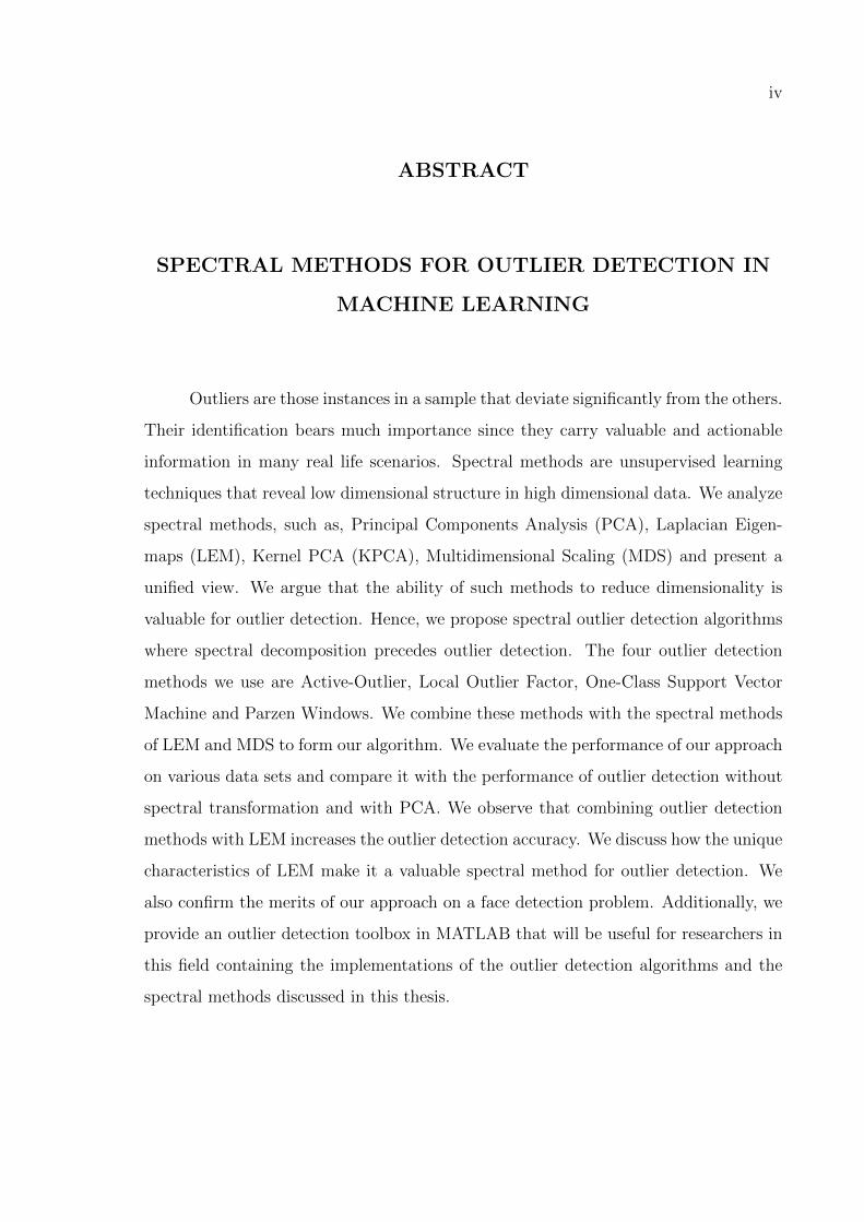
Outliers are those instances in a sample that deviate significantly from the others.

Their identification bears much importance since they carry valuable and actionable

information in many real life scenarios. Spectral methods are unsupervised learning

techniques that reveal low dimensional structure in high dimensional data. We analyze

spectral methods, such as, Principal Components Analysis (PCA), Laplacian Eigen-

maps (LEM), Kernel PCA (KPCA), Multidimensional Scaling (MDS) and present a

unified view. We argue that the ability of such methods to reduce dimensionality is

valuable for outlier detection. Hence, we propose spectral outlier detection algorithms

where spectral decomposition precedes outlier detection. The four outlier detection

methods we use are Active-Outlier, Local Outlier Factor, One-Class Support Vector

Machine and Parzen Windows. We combine these methods with the spectral methods

of LEM and MDS to form our algorithm. We evaluate the performance of our approach

on various data sets and compare it with the performance of outlier detection without

spectral transformation and with PCA. We observe that combining outlier detection

methods with LEM increases the outlier detection accuracy. We discuss how the unique

characteristics of LEM make it a valuable spectral method for outlier detection. We

also confirm the merits of our approach on a face detection problem. Additionally, we

provide an outlier detection toolbox in MATLAB that will be useful for researchers in

this field containing the implementations of the outlier detection algorithms and the

spectral methods discussed in this thesis.

v

OZET

YAPAY OGRENMEDE AYKIRILIK SEZIMI ICIN

IZGESEL YONTEMLER

Aykırılıklar verinin genelinden onemli farklılık gosteren orneklerdir. Gercek

yasamda karsımıza cıkan pek cok uygulamada aykırı orneklerin bulunması hem kavram-

sal hem de eylemsel acıdan degerli bilgi tasıdıkları icin onemlidir. Izgesel yontemler

yuksek boyutlu verilerdeki dusuk boyutlu yapıları ortaya cıkarabilen gozetimsiz ogrenme

yaklasımlarıdır. Bu yontemlerden Temel Bilesenler Cozumlemesi (TBC), Laplasyen

Ozharitalar (LOH) ve Cok Boyutlu Olcekleme incelenerek ortak bir catı altında sunul-

maktadır. Bu calısmada, izgesel yontemlerin boyut dusurme ozelliklerinin aykırılık bul-

makta degerli oldugu one surulmekte ve aykırılık bulma oncesinde izgesel yaklasımla

veriyi donusturen izgesel aykırılık bulma yontemi onerilmektedir. Etkin-Aykırı, Yerel

Aykırılık Etkeni, Tek Sınıflı Karar Vektor Makineleri ve Parzen Pencereleri aykırılık

bulma yontemleri olarak kullanılmakta ve bu yontemler Temel Bilesenler Cozumlemesi

(TBC), Laplasyen Ozharitalar (LOH) ve Cok Boyutlu Olcekleme’yle birlestirilerek

farklı veri kumeleri uzerinde aykırılık bulma basarımı sınanmaktadır. Deney sonucları

ozellikle LOH izgesel yonteminin basarımı artırdıgını gostermektedir. Sonrasında,

LOH yontemini aykırılık bulma icin degerli kılan ozgun ozellikleri tartısılmaktadır.

Onerdigimiz yaklasım yuz tanıma problemine de uygulanarak, one surulen yontemin

gecerliligi dogrulanmaktadır. Ayrıca, bu alandaki arastırmalarda kullanılmak icin,

aykırılık bulma ve izgesel yontemlerin gerceklenmesini iceren bir MATLAB kutuphanesi

de bu tez ile paylasılmaktadır.

vi

TABLE OF CONTENTS

ACKNOWLEDGEMENTS . . . . . . . . . . . . . . . . . . . . . . . . . . . . . iii

ABSTRACT . . . . . . . . . . . . . . . . . . . . . . . . . . . . . . . . . . . . . iv

OZET . . . . . . . . . . . . . . . . . . . . . . . . . . . . . . . . . . . . . . . . . v

LIST OF FIGURES . . . . . . . . . . . . . . . . . . . . . . . . . . . . . . . . . viii

LIST OF TABLES . . . . . . . . . . . . . . . . . . . . . . . . . . . . . . . . . . xii

LIST OF SYMBOLS . . . . . . . . . . . . . . . . . . . . . . . . . . . . . . . . . xv

LIST OF ACRONYMS/ABBREVIATIONS . . . . . . . . . . . . . . . . . . . . xvii

1. INTRODUCTION . . . . . . . . . . . . . . . . . . . . . . . . . . . . . . . . 1

1.1. Outlier Detection Problem Definition . . . . . . . . . . . . . . . . . . . 3

1.2. Outlier Detection Methods . . . . . . . . . . . . . . . . . . . . . . . . . 4

1.3. Outline of Thesis . . . . . . . . . . . . . . . . . . . . . . . . . . . . . . 6

2. OUTLIER DETECTION METHODS . . . . . . . . . . . . . . . . . . . . . 7

2.1. Outlier Detection by Active Learning . . . . . . . . . . . . . . . . . . . 7

2.2. LOF: Identifying Density-Based Local Outliers . . . . . . . . . . . . . . 10

2.2.1. Feature Bagging for Outlier Detection . . . . . . . . . . . . . . 13

2.3. One-Class Support Vector Machine . . . . . . . . . . . . . . . . . . . . 16

2.4. Parzen Windows . . . . . . . . . . . . . . . . . . . . . . . . . . . . . . 18

3. SPECTRAL METHODS . . . . . . . . . . . . . . . . . . . . . . . . . . . . . 21

3.1. Principal Components Analysis . . . . . . . . . . . . . . . . . . . . . . 22

3.2. Kernel Principal Components Analysis . . . . . . . . . . . . . . . . . . 23

3.3. Multidimensional Scaling . . . . . . . . . . . . . . . . . . . . . . . . . . 25

3.4. Laplacian Eigenmaps . . . . . . . . . . . . . . . . . . . . . . . . . . . . 25

3.5. Discussion . . . . . . . . . . . . . . . . . . . . . . . . . . . . . . . . . . 26

3.5.1. Approximating Dot Products or Euclidean Distances . . . . . . 28

3.5.2. Mean Centered KPCA is Equivalent to Classical MDS . . . . . 29

3.5.3. How LEM Differs from MDS and KPCA . . . . . . . . . . . . . 29

4. SPECTRAL OUTLIER DETECTION . . . . . . . . . . . . . . . . . . . . . 30

4.1. The Idea . . . . . . . . . . . . . . . . . . . . . . . . . . . . . . . . . . . 30

4.2. Related Work . . . . . . . . . . . . . . . . . . . . . . . . . . . . . . . . 32

vii

5. EXPERIMENTS . . . . . . . . . . . . . . . . . . . . . . . . . . . . . . . . . 34

5.1. Evaluated Methods and Implementation Notes . . . . . . . . . . . . . . 34

5.2. Synthetic Data . . . . . . . . . . . . . . . . . . . . . . . . . . . . . . . 35

5.3. Real Data . . . . . . . . . . . . . . . . . . . . . . . . . . . . . . . . . . 43

5.3.1. Data Sets . . . . . . . . . . . . . . . . . . . . . . . . . . . . . . 44

5.4. Face Detection . . . . . . . . . . . . . . . . . . . . . . . . . . . . . . . 78

6. CONCLUSIONS AND FUTURE WORK . . . . . . . . . . . . . . . . . . . . 81

APPENDIX A: OUTLIER DETECTION TOOLBOX IN MATLAB . . . . . . 84

REFERENCES . . . . . . . . . . . . . . . . . . . . . . . . . . . . . . . . . . . . 88

viii

LIST OF FIGURES

Figure 2.1. Active-Outlier method. . . . . . . . . . . . . . . . . . . . . . . . . 10

Figure 2.2. Example data set. . . . . . . . . . . . . . . . . . . . . . . . . . . . 11

Figure 2.3. LOF method. . . . . . . . . . . . . . . . . . . . . . . . . . . . . . 13

Figure 2.4. Feature bagging method. . . . . . . . . . . . . . . . . . . . . . . . 14

Figure 2.5. Feature bagging breadth-first combination. . . . . . . . . . . . . . 15

Figure 2.6. Feature bagging cumulative-sum combination. . . . . . . . . . . . 16

Figure 2.7. Parzen Windows algorithm. . . . . . . . . . . . . . . . . . . . . . 20

Figure 3.1. LEM, KPCA, KPCA-Mean centered and MDS transformations of

a synthetic sample with Gaussian kernel with σ = .1 and neighbor

count k = 2. . . . . . . . . . . . . . . . . . . . . . . . . . . . . . . 28

Figure 4.1. Boundary learned by Active-Outlier on a synthetic circular data set. 31

Figure 4.2. Boundary learned by Active-Outlier on a synthetic circular data

set after KPCA with Gaussian kernel (k = 2, σ = .4). . . . . . . . 32

Figure 4.3. Spectral outlier detection algorithm. . . . . . . . . . . . . . . . . . 33

Figure 5.1. Synthetic data set 1. . . . . . . . . . . . . . . . . . . . . . . . . . 37

Figure 5.2. Synthetic data set 2. . . . . . . . . . . . . . . . . . . . . . . . . . 37

ix

Figure 5.3. Outlier scores and discriminants for outlier count 2, 10, 50 with the

Active-Outlier method. . . . . . . . . . . . . . . . . . . . . . . . . 38

Figure 5.4. Outlier scores and discriminants for outlier count 2, 10, 50 with the

LOF method. . . . . . . . . . . . . . . . . . . . . . . . . . . . . . 40

Figure 5.5. Outlier scores and discriminants for outlier count 2, 10, 50 with the

Parzen Windows method. . . . . . . . . . . . . . . . . . . . . . . . 41

Figure 5.6. Outlier scores and discriminants for outlier count 2, 10, 50 with the

One-Class Support Vector Machine. . . . . . . . . . . . . . . . . . 42

Figure 5.7. AUC vs. kernel type on Optdigits data set. . . . . . . . . . . . . . 48

Figure 5.8. AUC vs. kernel type on Shuttle data set. . . . . . . . . . . . . . . 49

Figure 5.9. AUC vs. neighbor count on Optdigits data set with constant kernel. 50

Figure 5.10. AUC vs. neighbor count on Shuttle data set with constant kernel. 50

Figure 5.11. AUC vs. neighbor count on Optdigits data set with Gaussian kernel. 51

Figure 5.12. AUC vs. neighbor count on Shuttle data set with Gaussian kernel. 51

Figure 5.13. AUC vs. neighbor count on Optdigits data set with quadratic kernel. 52

Figure 5.14. AUC vs. neighbor count on Shuttle data set with quadratic kernel. 52

Figure 5.15. AUC vs. input dimensionality on Optdigits data set. . . . . . . . . 53

Figure 5.16. AUC vs. input dimensionality on Shuttle data set. . . . . . . . . . 54

x

Figure 5.17. Plots of AUCs for the semi-supervised case. . . . . . . . . . . . . . 56

Figure 5.18. Plots of AUCs for the unsupervised case. . . . . . . . . . . . . . . 57

Figure 5.19. Plots of AUCs for spectral outlier detection with PCA for the semi-

supervised case. . . . . . . . . . . . . . . . . . . . . . . . . . . . . 60

Figure 5.20. Plots of AUCs for spectral outlier detection with PCA for the un-

supervised case. . . . . . . . . . . . . . . . . . . . . . . . . . . . . 60

Figure 5.21. Plots of AUCs for spectral outlier detection with LEM for the semi-

supervised case. . . . . . . . . . . . . . . . . . . . . . . . . . . . . 64

Figure 5.22. Plots of AUCs for spectral outlier detection with LEM for the un-

supervised case. . . . . . . . . . . . . . . . . . . . . . . . . . . . . 64

Figure 5.23. Plots of AUCs for spectral outlier detection with MDS for the semi-

supervised case. . . . . . . . . . . . . . . . . . . . . . . . . . . . . 65

Figure 5.24. Plots of AUCs for spectral outlier detection with MDS for the un-

supervised case. . . . . . . . . . . . . . . . . . . . . . . . . . . . . 68

Figure 5.25. Plots of AUCs for AO with different spectral methods for the semi-

supervised case. . . . . . . . . . . . . . . . . . . . . . . . . . . . . 70

Figure 5.26. Plots of AUCs for AO with different spectral methods for the un-

supervised case. . . . . . . . . . . . . . . . . . . . . . . . . . . . . 70

Figure 5.27. Plots of AUCs for LOF with different spectral methods for the

semi-supervised case. . . . . . . . . . . . . . . . . . . . . . . . . . 72

xi

Figure 5.28. Plots of AUCs for LOF with different spectral methods for the

unsupervised case. . . . . . . . . . . . . . . . . . . . . . . . . . . . 72

Figure 5.29. Plots of AUCs for SVM with different spectral methods for the

semi-supervised case. . . . . . . . . . . . . . . . . . . . . . . . . . 73

Figure 5.30. Plots of AUCs for SVM with different spectral methods for the

unsupervised case. . . . . . . . . . . . . . . . . . . . . . . . . . . . 73

Figure 5.31. Plots of AUCs for PW with different spectral methods for the semi-

supervised case. . . . . . . . . . . . . . . . . . . . . . . . . . . . . 74

Figure 5.32. Plots of AUCs for PW with different spectral methods for the un-

supervised case. . . . . . . . . . . . . . . . . . . . . . . . . . . . . 74

Figure 5.33. CBCL Face data set reduced to two dimensions with PCA. . . . . 79

Figure 5.34. CBCL Face data set reduced to two dimensions with LEM (Gaus-

sian kernel, k = 3 and σ = 101.70). . . . . . . . . . . . . . . . . . 80

Figure A.1. Spectral methods demonstration demo script’s first screen where

points and kernel parameters are selected. . . . . . . . . . . . . . . 85

Figure A.2. Spectral methods demonstration demo script’s second screen where

spectral transformations are plotted. . . . . . . . . . . . . . . . . . 85

Figure A.3. Outlier detection toolbox demonstration od script’s GUI. . . . . . 86

xii

LIST OF TABLES

Table 1.1. Summary of outlier detection methods. . . . . . . . . . . . . . . . 6

Table 3.1. Comparison of cost functions optimized by dimensionality reduction

methods. . . . . . . . . . . . . . . . . . . . . . . . . . . . . . . . . 27

Table 5.1. Data sets used in the experiments. . . . . . . . . . . . . . . . . . . 47

Table 5.2. Average values and standard deviations of AUCs for the semi-

supervised case. . . . . . . . . . . . . . . . . . . . . . . . . . . . . 55

Table 5.3. Average values and standard deviations of AUCs for the unsuper-

vised case. . . . . . . . . . . . . . . . . . . . . . . . . . . . . . . . 56

Table 5.4. Wins/ties/losses of each algorithm with 5× 2 cv F test. . . . . . . 57

Table 5.5. Average values and standard deviations of AUCs for spectral outlier

detection with PCA, semi-supervised case. . . . . . . . . . . . . . . 58

Table 5.6. Average values and standard deviations of AUCs for spectral outlier

detection with PCA, unsupervised case. . . . . . . . . . . . . . . . 59

Table 5.7. Wins/ties/losses of outlier detection methods combined with PCA

with 5× 2 cv F test. . . . . . . . . . . . . . . . . . . . . . . . . . . 59

Table 5.8. Average values and standard deviations of AUCs for spectral outlier

detection with LEM, semi-supervised case. . . . . . . . . . . . . . 62

xiii

Table 5.9. Average values and standard deviations of AUCs for spectral outlier

detection with LEM, unsupervised case. . . . . . . . . . . . . . . . 63

Table 5.10. Wins/ties/losses of outlier detection methods combined with LEM

with 5× 2 cv F test. . . . . . . . . . . . . . . . . . . . . . . . . . . 65

Table 5.11. Average values and standard deviations of AUCs for spectral outlier

detection with MDS, semi-supervised case. . . . . . . . . . . . . . 66

Table 5.12. Average values and standard deviations of AUCs for spectral outlier

detection with MDS, unsupervised case. . . . . . . . . . . . . . . . 67

Table 5.13. Wins/ties/losses of outlier detection methods combined with MDS. 68

Table 5.14. Average ranks of outlier detection methods. . . . . . . . . . . . . . 69

Table 5.15. Significant differences between outlier detection methods for each

spectral method for the semi-supervised case. . . . . . . . . . . . . 69

Table 5.16. Significant differences between outlier detection methods for each

spectral method for the unsupervised case. . . . . . . . . . . . . . 69

Table 5.17. Average ranks of spectral methods with respect to outlier detection

methods. . . . . . . . . . . . . . . . . . . . . . . . . . . . . . . . . 71

Table 5.18. Significant differences between spectral methods for each outlier

detection method for the semi-supervised case. . . . . . . . . . . . 75

Table 5.19. Significant differences between spectral methods for each outlier

detection method for the unsupervised case. . . . . . . . . . . . . . 75

xiv

Table 5.20. Wins/ties/losses of outlier detection methods combined with spec-

tral methods for the semi-supervised case. . . . . . . . . . . . . . . 76

Table 5.21. Wins/ties/losses of outlier detection methods combined with spec-

tral method for the unsupervised case. . . . . . . . . . . . . . . . . 77

xv

LIST OF SYMBOLS

B Background distribution

B Dot product matrix

Ci Class i

C Cost function

d Number of input dimensions

D Distribution

D Diagonal matrix of row/column sums

e(x) Error function

E Distance matrix

g(x) Model/Classifier

G(x) Set of classifiers

H Subset of input space

H Set of subsets of input space

k Neighbor count

kmin Minimum neighbor count

kmax Maximum neighbor count

K Kernel function

L Lagrangian function

K Kernel matrix

m Number of output dimensions

M Number of combined/trained methods

M(G|x) Margin for the instance x with classifiers in set G

N Number of instances

p(x) Probability function

p(x) Estimated probability

r Output vector

s Variance

S Similarity matrix

xvi

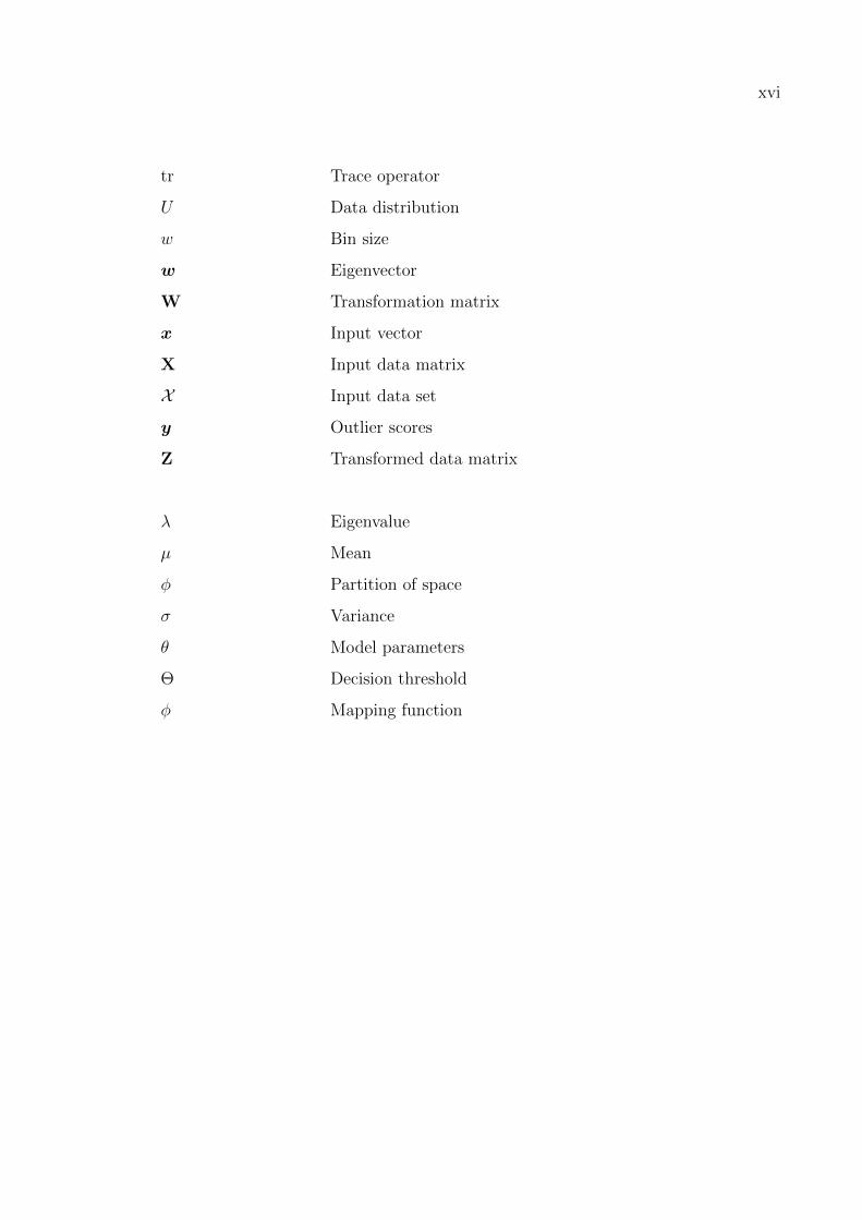
tr Trace operator

U Data distribution

w Bin size

w Eigenvector

W Transformation matrix

x Input vector

X Input data matrix

X Input data set

y Outlier scores

Z Transformed data matrix

λ Eigenvalue

µ Mean

φ Partition of space

σ Variance

θ Model parameters

Θ Decision threshold

φ Mapping function

xvii

LIST OF ACRONYMS/ABBREVIATIONS

AO Active-Outlier

ANOVA Analysis of Variances

AUC Area Under the Curve

CV Cross Validation

GUI Graphical User Interface

KPCA Kernel Principal Components Analysis

LEM Laplacian Eigenmaps

LOF Local Outlier Factor

MDS Multidimensional Scaling

ML Machine Learning

PCA Principal Components Analysis

PR Precision-Recall

PW Parzen Windows

ROC Receiver Operating Characteristic

SS Semi-Supervised

SVM One-Class Support Vector Machine

US Unsupervised

1

1. INTRODUCTION

Machine learning (ML) is the engineering of methods that enable machines, i.e.,

computers to adapt their behavior based on empirical data. ML analyzes example data

or past experience and uses the theory of statistics to build mathematical models to

predict events in the future and/or describe the observed behavior [1]. ML methods are

generally categorized according to the nature of the learning problem or the statistical

assumptions they make. According to the nature of the learning problem, ML methods

can be classified as supervised or unsupervised. The following paragraphs are largely

adopted from [1].

In supervised learning, the data set contains the actual output value for each

input instance. For example, for the task of determining if a person is a high-risk

customer for giving loans, we have past customer attributes together with the label for

each customer indicating if they are a high-risk customer or not. Here our training set

consists of input pairs

X = {(x(t), r(t))}Nt=1 (1.1)

where x(t) ∈ Rd is the vector denoting instance t in our sample of size N and r(t)

specifies the output for the instance. If r(t) takes only discrete values, such as 1 for high-

risk and otherwise 0, this problem is called a classification problem. In classification

problems, we aim to predict the class that a future instance belongs to by making

inference from the past data X . For a classification problem with m classes denoted

as Ci, i = 1, ...,m, r(t) is m-dimensional and

r(t)i =

1 if x(t) ∈ Ci0 if x(t) ∈ Cj, j 6= i

(1.2)

2

If there are only two classes, which is called a binary classification problem, one class

is chosen as positive with r(t) = 1 and the other as negative class with r(t) = 0. If

the output values are continuous, it is a regression problem. For instance, estimating

the life expectancy of a person from his/her personal data is a regression problem.

In supervised learning, our aim is to learn a model g(x|θ) where θ are the model pa-

rameters that we need to estimate from the sample X . We look for θ∗ that minimize

a loss function measuring the difference between actual r(t) values and our model’s

predictions g(x(t)|θ). For classification problems, g(x|θ) divides the input space into

regions for each class and the boundaries that separate classes are called discriminants.

In unsupervised learning, we only have the input data x(t) and no r(t). The aim

is to find patterns, regularities or groupings in data. This type of learning is known

as density estimation in statistics. An important problem in unsupervised learning is

clustering, that is, extracting a mapping function from training set that assigns each

instance to a group. For example, discovering customer profiles from customer data

can be achieved by clustering. The middle road between supervised and unsupervised

learning is where only labels or output values for a subset of the training set are avail-

able.

Every ML method makes some statistical assumptions in order to solve an oth-

erwise intractable problem. Parametric methods assume that the sample X is drawn

from a distribution and estimate the values of the parameters of this distribution. In

the case of classification, every class conditional density p(x|Ci) is assumed to be of

some form and p(x|Ci), p(Ci) densities are estimated to calculate the posterior prob-

ability p(Ci|x) using Bayes’ rule to make our predictions. Parametric methods are

advantageous since learning is reduced to estimating the values of a small number of

parameters. However, these assumptions may not always hold and we need to turn

to non-parametric methods. In non-parametric methods, we only assume that similar

instances have similar outputs and our algorithm finds similar instances from X and

uses them to predict the right output. However, this lack of assumptions comes with

a price on time and space complexity. Non-parametric methods need to store the past

3

data and carry out extra computation to find the similar instances whereas paramet-

ric methods only store the values of a few parameters and are less time and memory

consuming.

1.1. Outlier Detection Problem Definition

In this thesis, we deal with the problem of outlier detection. Outlier (or anomaly)

is just another one of those concepts where we all know one when we see one. However,

our every attempt at delineating a formal definition falls short, perhaps because of

the unconscious processes of our brain in identifying outliers. One widely referenced

definition by Grubbs [2] is as follows.

“An outlying observation, or outlier, is one that appears to deviate markedlyfrom other members of the sample in which it occurs.”

Although it is quite hard to frame outlierness without resorting to ambiguous concepts

such as ”deviation”, the detection of outliers bears high importance since such outliers

convey valuable and actionable information in many real life scenarios. An outlier

may be an attack in a network, a potential fault in a machine or denote a cancerous

tumor [3]. Apart from the practical applications, outliers also have theoretical value

from the perspective of learning theory. In his inspiring book Society of Mind [4],

Minsky elaborates on various types of learning and also mentions the importance of

outliers. Uniframing, as called by Minsky, refers to our abilities of combining several

distinct descriptions into one and inferring a general model that largely explains our

observations. However, uniframing does not always work, since some of our experiences

may lack a common ground to be included in our established models. In that case,

another type of learning, accumulation, plays a role where incompatible observations

are collected and stored as exceptions to our models. This dual strategy of learning en-

ables us to efficiently create descriptions of things without getting lost in details of the

individual objects and prevents our models from losing their generalization capabilities

by wrongly incorporating examples that deviate from the description into the model.

In such a learning method, detecting outliers bears importance since it determines the

4

learning type to employ for the observation in question.

From a more formal perspective, outlier detection can be considered as a classifi-

cation problem. We want to calculate a function g(x) that predicts if an instance is an

outlier. This function may provide hard decisions, e.g., 0 for typicals and 1 for outliers,

or return a real number corresponding to the degree of being an outlier. However, the

availability of labels as typical vs. outlier is not always possible. We may have only

a sample from the class of typical examples or a mixed sample without any labels.

Hence, outlier detection is sometimes a supervised learning problem and in some cases,

an unsupervised or a semi-supervised learning problem.

Outlier detection differs from classification in a few aspects. Class distributions in

outlier detection problems are highly unbalanced, since the outlier instances are much

fewer compared to the typical ones. Additionally, classification costs are not symmetric.

Generally, the misclassification of an outlier as typical, e.g., missing a cancerous tumor,

is more costly than assigning a typical instance as outlier. Another consideration for

outlier detection problems is that the noisy instances are usually similar to the outliers

and they may be hard to remove or to disregard. Lastly, it is usually the case that we

do not have labeled outlier instances. These characteristics of outlier detection limit

the applicability of classification methods and call for specially designed algorithms.

1.2. Outlier Detection Methods

In this section, we present a taxonomy of outlier detection methods; see [3] for a

more extended review.

Discriminant based methods learn a discriminative model over the input space,

separating outliers and the typical instances. The most distinctive property of these

methods is the requirement that data be labeled as typical or outlier and this re-

quirement limits their applicability. However, once labeled data are available, the

well-established theory of classification and the vast number of diverse methods can be

5

used. These methods can be further categorized into two. Two-class methods require

data labeled as typical vs. outlier, while one-class methods use only the sample of typ-

icals to learn a boundary that discriminates typical and outlier instances. There are

outlier detection methods that use multi-layered perceptrons trained with the sample

of typicals and identify an instance as outlier if the network rejects it [5,6]. Autoasso-

ciative networks, adaptive resonance theory and radial basis function based techniques

are also proposed [7–9]. Rule based methods extract rules that describe typical behav-

ior and detect outliers based on these rules [10]. Support Vector Machines have been

applied to outlier detection as one-class methods [11, 12]. Kernel Fisher discriminants

have also been used as a one-class method for outlier detection [13].

Density based methods assume that the outliers occur far from the typical in-

stances, that is, in low density regions of the input space. Estimating the density

can be carried out using parametric methods that assume an underlying model, semi-

parametric ones such as clustering methods, or non-parametric methods like Parzen

Windows [14]. In parametric methods, sample of typical instances is assumed to obey a

known distribution and statistical tests are used for identifying outliers [15,16]. There

are also regression based methods where the residuals for test instances are used as out-

lier scores [17]. Semi-parametric methods assume a mixture of parametric distributions

for the typical and/or outlier sample and use statistical tests to find outliers [18, 19].

Non-parametric methods use histogram based or kernel based techniques to estimate

densities to calculate outlier scores [20, 21]. Then, these estimated densities are trans-

formed into a measure of being an outlier. Semi-parametric clustering based methods

make different assumptions to decide on the outliers. In [22], an instance that does not

belong to any cluster is deemed outlier while in [23], an instance that is far from any

cluster center and/or in a small sized cluster is considered an outlier. Non-parametric

nearest neighbor based methods use different measures to determine the outliers, such

as distance to the kth neighbor [24], the sum of distances to the k nearest neighbors [25]

or the number of neighbors in the neighborhood of a certain size [26]. There are also

techniques that take into account the relative densities around an instance to calculate

an outlier score such as the Local Outlier Factor (LOF) method [27].

6

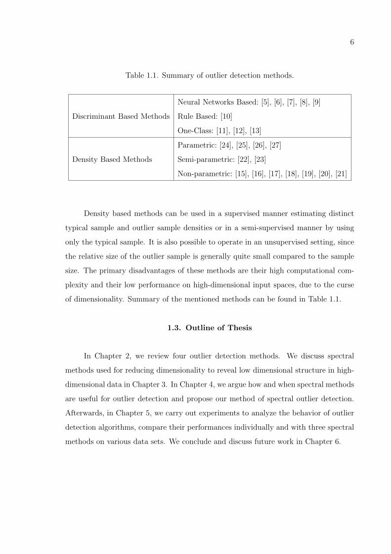
Table 1.1. Summary of outlier detection methods.

Discriminant Based Methods

Neural Networks Based: [5], [6], [7], [8], [9]

Rule Based: [10]

One-Class: [11], [12], [13]

Density Based Methods

Parametric: [24], [25], [26], [27]

Semi-parametric: [22], [23]

Non-parametric: [15], [16], [17], [18], [19], [20], [21]

Density based methods can be used in a supervised manner estimating distinct

typical sample and outlier sample densities or in a semi-supervised manner by using

only the typical sample. It is also possible to operate in an unsupervised setting, since

the relative size of the outlier sample is generally quite small compared to the sample

size. The primary disadvantages of these methods are their high computational com-

plexity and their low performance on high-dimensional input spaces, due to the curse

of dimensionality. Summary of the mentioned methods can be found in Table 1.1.

1.3. Outline of Thesis

In Chapter 2, we review four outlier detection methods. We discuss spectral

methods used for reducing dimensionality to reveal low dimensional structure in high-

dimensional data in Chapter 3. In Chapter 4, we argue how and when spectral methods

are useful for outlier detection and propose our method of spectral outlier detection.

Afterwards, in Chapter 5, we carry out experiments to analyze the behavior of outlier

detection algorithms, compare their performances individually and with three spectral

methods on various data sets. We conclude and discuss future work in Chapter 6.

7

2. OUTLIER DETECTION METHODS

2.1. Outlier Detection by Active Learning

Supervised, classification based Active-Outlier (AO) method [28] is an ensemble

of classifiers that are trained on selectively sampled subsets of training data in order

to learn a tight boundary around typical instances. When compared to outlier detec-

tion methods based on probabilistic or nearest-neighbor approaches, the Active-Outlier

method requires much less computation since it does not need the training data in the

testing phase and also provides a much more rational and semantic explanation for

being an outlier.

Assuming that our data is drawn from a distribution U , our purpose is to find the

partition π with the minimum size that covers all the instances from U and none of the

other instances; these latter are assumed to originate from a background distribution

B. The error for this unsupervised learning problem can be defined as follows:

eU,B(π) =1

2(px∼U(x /∈ π) + px∼B(x ∈ π)) (2.1)

We may convert the above unsupervised learning problem to a classification problem

by drawing instances evenly from U and B and by considering data and background

distribution to be labelled as different classes. Let us assume that instances X =

{(x(t), r(t))}Nt=1, where r(t) ∈ {0, 1}, are drawn from a distribution D, our purpose is

find a classifier g : x→ r that minimizes the classification error:

eD(g) = px,r∼D(g(x) 6= r) (2.2)

Let us say D is composed of instances from U and B in equal sizes and that we

label instances from U with class label 1 and instances from B with class label 0.

Then, minimizing the classification error is equivalent to minimizing the error for the

8

unsupervised learning problem:

eD(g) = px,r∼D(g(x) 6= 0|r = 0)px,r∼D(r = 0) (2.3)

+ px,r∼D(g(x) 6= 1|r = 1)px,r∼D(r = 1) (2.4)

= 0.5px∼B(x ∈ π) + 0.5px∼U(x /∈ π) (2.5)

With the above reduction, the outlier detection problem can be interpreted as a clas-

sification problem where we look for an accurate classifier that discriminates between

the labeled training instances which are considered typical and the artificially gener-

ated instances that we insert into training data as potential outliers. In this manner,

the classifier learns a tight boundary around the sample of typical instances and any

instance outside is deemed an outlier. However, the accuracy of this approach relies

heavily on the quality of background distribution. In order to decrease the dependence

of the method on the background distribution, authors employ the active learning ap-

proach where the training instances given to the classifier are chosen dynamically. For

the specific case of Active-Outlier, the next instance is drawn from regions close to the

classification boundaries in order to have the boundary as tight as possible. Moreover,

instead of training a single classifier on the generated data set, an ensemble of classifiers

is formed by training multiple classifiers consecutively on selectively sampled subsets

of data. This combination of active learning and sampling based on margin is called

ensemble-based minimum margin active learning [28].

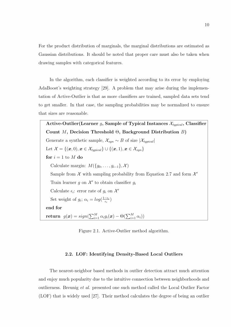
The pseudo-code of the algorithm is given in Figure 2.1. Given a data set con-

taining typical instances, in the first step, synthetically generated data are added as

potential outliers to the data set. In the selective sampling step, margins, indicating

the confidence of classifier in its decision, are calculated for each instance. A new data

set is formed by drawing a sample from our original data set in a manner that gives

higher probability to instances with low margin. Then, the next classifier is trained on

this new data set and these selective sampling and training steps are repeated as many

times as necessary to form an ensemble of classifiers. In testing, we apply majority

voting on the classifier outputs.

9

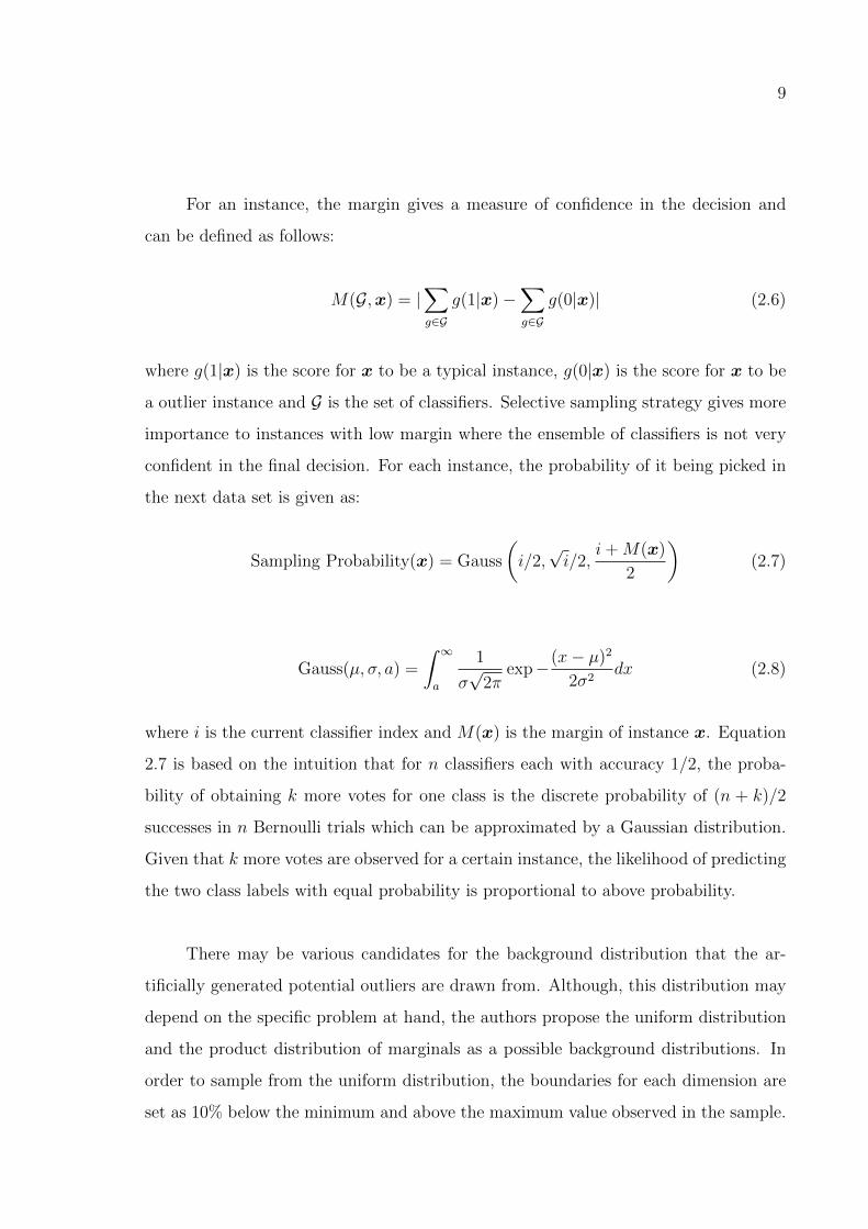
For an instance, the margin gives a measure of confidence in the decision and

can be defined as follows:

M(G,x) = |∑g∈G

g(1|x)−∑g∈G

g(0|x)| (2.6)

where g(1|x) is the score for x to be a typical instance, g(0|x) is the score for x to be

a outlier instance and G is the set of classifiers. Selective sampling strategy gives more

importance to instances with low margin where the ensemble of classifiers is not very

confident in the final decision. For each instance, the probability of it being picked in

the next data set is given as:

Sampling Probability(x) = Gauss

(i/2,√i/2,

i+M(x)

2

)(2.7)

Gauss(µ, σ, a) =

∫ ∞a

1

σ√

2πexp−(x− µ)2

2σ2dx (2.8)

where i is the current classifier index and M(x) is the margin of instance x. Equation

2.7 is based on the intuition that for n classifiers each with accuracy 1/2, the proba-

bility of obtaining k more votes for one class is the discrete probability of (n + k)/2

successes in n Bernoulli trials which can be approximated by a Gaussian distribution.

Given that k more votes are observed for a certain instance, the likelihood of predicting

the two class labels with equal probability is proportional to above probability.

There may be various candidates for the background distribution that the ar-

tificially generated potential outliers are drawn from. Although, this distribution may

depend on the specific problem at hand, the authors propose the uniform distribution

and the product distribution of marginals as a possible background distributions. In

order to sample from the uniform distribution, the boundaries for each dimension are

set as 10% below the minimum and above the maximum value observed in the sample.

10

For the product distribution of marginals, the marginal distributions are estimated as

Gaussian distributions. It should be noted that proper care must also be taken when

drawing samples with categorical features.

In the algorithm, each classifier is weighted according to its error by employing

AdaBoost’s weighting strategy [29]. A problem that may arise during the implemen-

tation of Active-Outlier is that as more classifiers are trained, sampled data sets tend

to get smaller. In that case, the sampling probabilities may be normalized to ensure

that sizes are reasonable.

Active-Outlier(Learner g, Sample of Typical Instances Xtypical, Classifier

Count M , Decision Threshold Θ, Background Distribution B)

Generate a synthetic sample, Xsyn ∼ B of size |Xtypical|

Let X = {(x, 0),x ∈ Xtypical} ∪ {(x, 1),x ∈ Xsyn}

for i = 1 to M do

Calculate margin: M({g0, . . . , gi−1},X )

Sample from X with sampling probability from Equation 2.7 and form X ′

Train learner g on X ′ to obtain classifier gi

Calculate εi: error rate of gi on X ′

Set weight of gi; αi = log(1−εiεi

)

end for

return g(x) = sign(∑M

i=1 αigi(x)−Θ(∑M

i=1 αi))

Figure 2.1. Active-Outlier method algorithm.

2.2. LOF: Identifying Density-Based Local Outliers

The nearest-neighbor based methods in outlier detection attract much attention

and enjoy much popularity due to the intuitive connection between neighborhoods and

outlierness. Breunig et al. presented one such method called the Local Outlier Factor

(LOF) that is widely used [27]. Their method calculates the degree of being an outlier

11

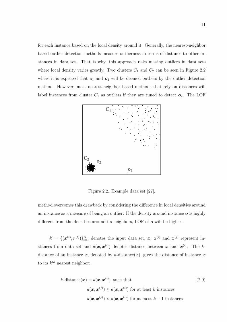
for each instance based on the local density around it. Generally, the nearest-neighbor

based outlier detection methods measure outlierness in terms of distance to other in-

stances in data set. That is why, this approach risks missing outliers in data sets

where local density varies greatly. Two clusters C1 and C2 can be seen in Figure 2.2

where it is expected that o1 and o2 will be deemed outliers by the outlier detection

method. However, most nearest-neighbor based methods that rely on distances will

label instances from cluster C1 as outliers if they are tuned to detect o2. The LOF

Figure 2.2. Example data set [27].

method overcomes this drawback by considering the difference in local densities around

an instance as a measure of being an outlier. If the density around instance o is highly

different from the densities around its neighbors, LOF of o will be higher.

X = {(x(t), r(t))}Nt=1 denotes the input data set, x, x(i) and x(j) represent in-

stances from data set and d(x,x(i)) denotes distance between x and x(i). The k-

distance of an instance x, denoted by k-distance(x), gives the distance of instance x

to its kth nearest neighbor:

k-distance(x) ≡ d(x,x(i)) such that (2.9)

d(x,x(j)) ≤ d(x,x(i)) for at least k instances

d(x,x(j)) < d(x,x(i)) for at most k − 1 instances

12

The k-distance neighborhood of an instance x, denoted by Nk(x), contains all the

instances that are closer to x than its k-distance(x) value:

Nk(x) = {x(t) ∈ X \ {x}|d(x,x(t)) < k-distance(x)} (2.10)

The reachability distance of an instance x with respect to another instance x(i) is the

distance between the two instances, but in order to prevent unnecessary fluctuations,

reachability distances are smoothed in k-distance neighborhoods by assigning the same

reachability distance to instances that are in the neighborhood of x(i):

reachdistk(x,x(i)) = max{k-distance(x(i)), d(x,x(i))} (2.11)

The local reachability density measures how easy it is to reach a certain instance and

is calculated as the inverse of the average reachability distances of instances in the

k-distance neighborhood:

lrdk(x) =|Nk(x)|∑

x(i)∈Nk(x)reachdistk(x,x(i))

(2.12)

After defining the local reachability density, we may move on to the final step where

we calculate the local outlier factor for each instance. We expect instances with high

variance between local reachability densities of its neighbors to take higher LOF values:

LOFk(x) =

∑x(i)∈Nk(x)

lrdk(x(i))

lrdk(x)

|Nk(x)|(2.13)

Each specific problem requires a separate parameter search step to find the op-

timum k value. Moreover, the LOF values are quite sensitive to the value of k and

may exhibit unstable behavior as k changes. In order to minimize the instability of the

LOF values, authors propose calculating LOF values for various k values and taking

the maximum of them for each instance. Although, it is possible to apply different

heuristics to combine multiple LOF values, taking the maximum gives more impor-

13

tance to the LOF values individually and does not risk missing any possible outliers.

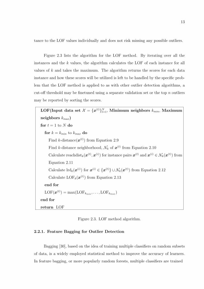
Figure 2.3 lists the algorithm for the LOF method. By iterating over all the

instances and the k values, the algorithm calculates the LOF of each instance for all

values of k and takes the maximum. The algorithm returns the scores for each data

instance and how these scores will be utilized is left to be handled by the specific prob-

lem that the LOF method is applied to as with other outlier detection algorithms, a

cut-off threshold may be finetuned using a separate validation set or the top n outliers

may be reported by sorting the scores.

LOF(Input data set X = {x(t)}Nt=1, Minimum neighbors kmin, Maximum

neighbors kmax)

for t = 1 to N do

for k = kmin to kmax do

Find k-distance(x(t)) from Equation 2.9

Find k-distance neighborhood, Nk of x(t) from Equation 2.10

Calculate reachdistk(x(t),x(i)) for instance pairs x(t) and x(i) ∈ Nk(x(t)) from

Equation 2.11

Calculate lrdk(x(i)) for x(i) ∈ {x(t)} ∪ Nk(x(t)) from Equation 2.12

Calculate LOFk(x(t)) from Equation 2.13

end for

LOF(x(t)) = max(LOFkmin, . . . ,LOFkmax)

end for

return LOF

Figure 2.3. LOF method algorithm.

2.2.1. Feature Bagging for Outlier Detection

Bagging [30], based on the idea of training multiple classifiers on random subsets

of data, is a widely employed statistical method to improve the accuracy of learners.

In feature bagging, or more popularly random forests, multiple classifiers are trained

14

on random feature subsets of data [31]. By using random subspaces, high dimensional

data can be more easily processed and the accuracy of the learner will be less affected

by the noisy features in the data set. Lazarevic et al. apply feature bagging to the

outlier detection problem and propose two alternatives to combine the outlier scores

[32]. These scores need not come from the same outlier detection method, since only

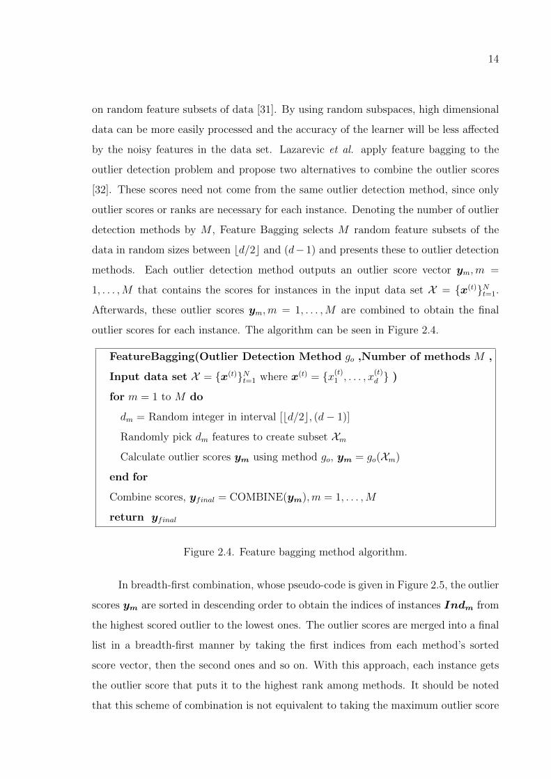
outlier scores or ranks are necessary for each instance. Denoting the number of outlier

detection methods by M , Feature Bagging selects M random feature subsets of the

data in random sizes between bd/2c and (d− 1) and presents these to outlier detection

methods. Each outlier detection method outputs an outlier score vector ym,m =

1, . . . ,M that contains the scores for instances in the input data set X = {x(t)}Nt=1.

Afterwards, these outlier scores ym,m = 1, . . . ,M are combined to obtain the final

outlier scores for each instance. The algorithm can be seen in Figure 2.4.

FeatureBagging(Outlier Detection Method go ,Number of methods M ,

Input data set X = {x(t)}Nt=1 where x(t) = {x(t)1 , . . . , x(t)d } )

for m = 1 to M do

dm = Random integer in interval [bd/2c, (d− 1)]

Randomly pick dm features to create subset XmCalculate outlier scores ym using method go, ym = go(Xm)

end for

Combine scores, yfinal = COMBINE(ym),m = 1, . . . ,M

return yfinal

Figure 2.4. Feature bagging method algorithm.

In breadth-first combination, whose pseudo-code is given in Figure 2.5, the outlier

scores ym are sorted in descending order to obtain the indices of instances Indm from

the highest scored outlier to the lowest ones. The outlier scores are merged into a final

list in a breadth-first manner by taking the first indices from each method’s sorted

score vector, then the second ones and so on. With this approach, each instance gets

the outlier score that puts it to the highest rank among methods. It should be noted

that this scheme of combination is not equivalent to taking the maximum outlier score

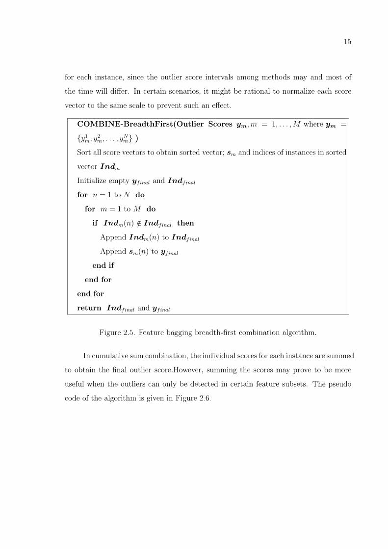
15

for each instance, since the outlier score intervals among methods may and most of

the time will differ. In certain scenarios, it might be rational to normalize each score

vector to the same scale to prevent such an effect.

COMBINE-BreadthFirst(Outlier Scores ym,m = 1, . . . ,M where ym =

{y1m, y2m, . . . , yNm} )

Sort all score vectors to obtain sorted vector; sm and indices of instances in sorted

vector Indm

Initialize empty yfinal and Indfinal

for n = 1 to N do

for m = 1 to M do

if Indm(n) /∈ Indfinal then

Append Indm(n) to Indfinal

Append sm(n) to yfinal

end if

end for

end for

return Indfinal and yfinal

Figure 2.5. Feature bagging breadth-first combination algorithm.

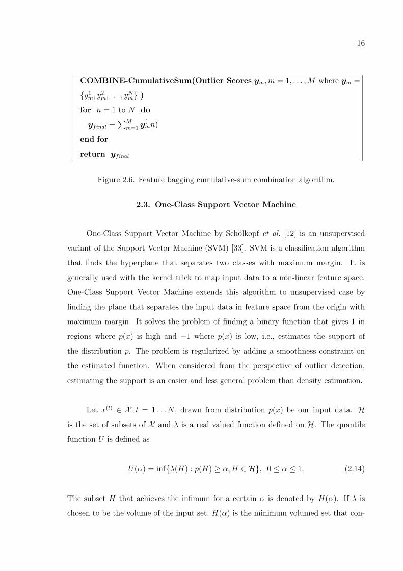
In cumulative sum combination, the individual scores for each instance are summed

to obtain the final outlier score.However, summing the scores may prove to be more

useful when the outliers can only be detected in certain feature subsets. The pseudo

code of the algorithm is given in Figure 2.6.

16

COMBINE-CumulativeSum(Outlier Scores ym,m = 1, . . . ,M where ym =

{y1m, y2m, . . . , yNm} )

for n = 1 to N do

yfinal =∑M

m=1 y(mn)

end for

return yfinal

Figure 2.6. Feature bagging cumulative-sum combination algorithm.

2.3. One-Class Support Vector Machine

One-Class Support Vector Machine by Scholkopf et al. [12] is an unsupervised

variant of the Support Vector Machine (SVM) [33]. SVM is a classification algorithm

that finds the hyperplane that separates two classes with maximum margin. It is

generally used with the kernel trick to map input data to a non-linear feature space.

One-Class Support Vector Machine extends this algorithm to unsupervised case by

finding the plane that separates the input data in feature space from the origin with

maximum margin. It solves the problem of finding a binary function that gives 1 in

regions where p(x) is high and −1 where p(x) is low, i.e., estimates the support of

the distribution p. The problem is regularized by adding a smoothness constraint on

the estimated function. When considered from the perspective of outlier detection,

estimating the support is an easier and less general problem than density estimation.

Let x(t) ∈ X , t = 1 . . . N , drawn from distribution p(x) be our input data. H

is the set of subsets of X and λ is a real valued function defined on H. The quantile

function U is defined as

U(α) = inf{λ(H) : p(H) ≥ α,H ∈ H}, 0 ≤ α ≤ 1. (2.14)

The subset H that achieves the infimum for a certain α is denoted by H(α). If λ is

chosen to be the volume of the input set, H(α) is the minimum volumed set that con-

17

tains a fraction α of the probability mass. For α = 1, H(1) contains the support of the

distribution p. If we can find the subset H for a specified α value, we can predict if a

test instance is an outlier by checking if it is out of H.

One-Class Support Vector algorithm chooses a λmeasure that controls the smooth-

ness of the estimated function instead of the volume of the set. The subset H is defined

by the function f that depends on the parameter of the hyperplane w, Hw = {x :

fw(x ≥ ρ)}, and the magnitude of the weight vector w is minimized, λ(Hw) = ||w||2.

Here, ρ is an offset parameterizing the hyperplane. The input data is mapped to a

non-linear space by function φ : X → F and the inner product in this new space

defines a kernel function K(x(i),x(j)) = φ(x(i))Tφ(x(j)). The aim is to find a function

f that returns 1 in a small region capturing most of the data and −1 elsewhere. This

is achieved by mapping the input data to the feature space and separating it from the

origin with maximum margin. The value of f for a test point is determined by the

side of the hyperplane it falls on in feature space. The binary function f is found by

solving the following quadratic program:

minw,ξ,ρ

1

2||w||2 +

1

νN

∑i

ξi − ρ

subject to (wTφ(x(i))) ≥ ρ− ξi, ξi ≥ 0.

(2.15)

Here, ν ∈ (0, 1] is a trade-off parameter that controls the effect of smoothness and the

error on the estimated function. The decision function f is then given as:

f(x) = sgn(wTφ(x)− ρ) (2.16)

where sgn(x) is the sign function that equals 1 for x ≥ 0. We write the Lagrangian by

using the multipliers αi, βi ≥ 0:

L(w, ξ, ρ,α,β) =1

2||w||2+

1

νN

∑i

ξi−ρ−∑i

αi(wTφ(x(i))−ρ+ξi)−

∑i

βiξi. (2.17)

18

We set the derivatives with respect to w, ξ and ρ equal to zero and get

w =∑i

αiφ(x(i)) (2.18)

αi =1

νN− βi,

∑i

αi = 1. (2.19)

All training instances x(i) that have αi ≥ 0 are called support vectors and they define

the hyperplane along with ρ. If we substitute w into the decision function f , we get

f(x) = sgn

(∑i

αiK(x(i),x)− ρ

). (2.20)

The support vectors are the instances that lie on the hyperplane and their ξi values

are zero. Therefore, we can calculate the value of ρ from any of the support vectors by

ρ = wTφ(x(i)) =∑j

αjK(x(j),x(i)). (2.21)

As we have pointed out earlier, ν controls the trade-off between error and smoothness.

If ν approaches zero, all the training instances are forced to lie on the same side of the

hyperplane since errors are punished severely. However, as ν increases, the smoothness

of the decision function becomes more and more important and more margin errors are

allowed. Scholkopf et al. show that ν is an upper bound on the fraction of outliers,

i.e., training instances that are not covered by the decision function [12]. It is also a

lower bound on the fraction of support vectors.

2.4. Parzen Windows

Parzen Windows (PW) is a non-parametric density estimation method [14]. While

a naive estimation for the density around an instance x can be calculated by counting

the number of instances that fall into the same neighborhood with it, Parzen Windows

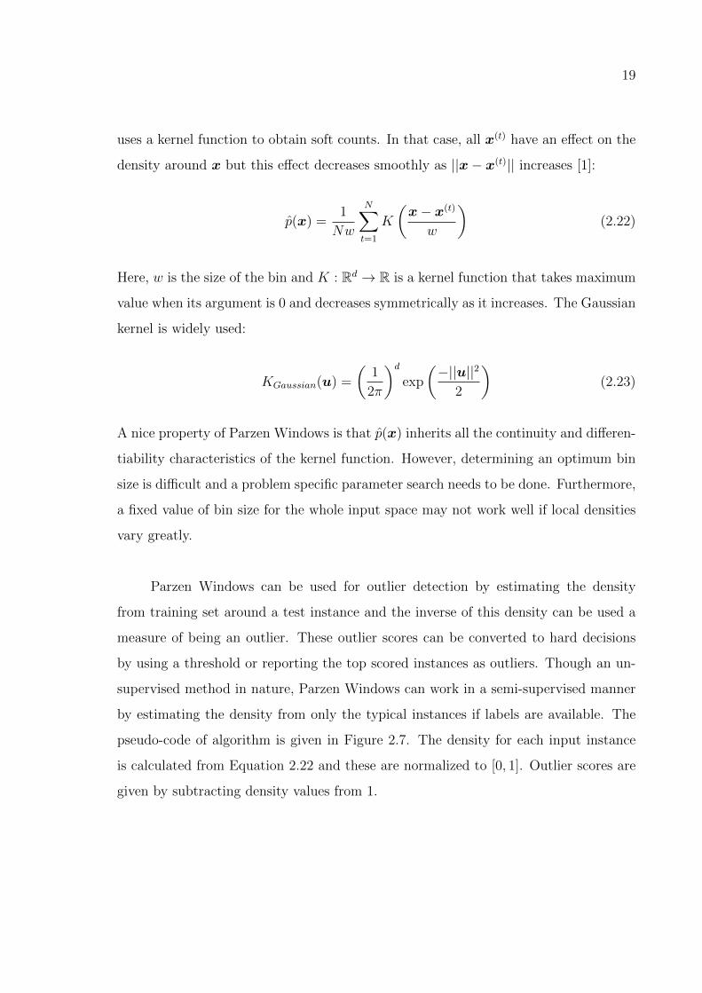
19

uses a kernel function to obtain soft counts. In that case, all x(t) have an effect on the

density around x but this effect decreases smoothly as ||x− x(t)|| increases [1]:

p(x) =1

Nw

N∑t=1

K

(x− x(t)

w

)(2.22)

Here, w is the size of the bin and K : Rd → R is a kernel function that takes maximum

value when its argument is 0 and decreases symmetrically as it increases. The Gaussian

kernel is widely used:

KGaussian(u) =

(1

2π

)dexp

(−||u||2

2

)(2.23)

A nice property of Parzen Windows is that p(x) inherits all the continuity and differen-

tiability characteristics of the kernel function. However, determining an optimum bin

size is difficult and a problem specific parameter search needs to be done. Furthermore,

a fixed value of bin size for the whole input space may not work well if local densities

vary greatly.

Parzen Windows can be used for outlier detection by estimating the density

from training set around a test instance and the inverse of this density can be used a

measure of being an outlier. These outlier scores can be converted to hard decisions

by using a threshold or reporting the top scored instances as outliers. Though an un-

supervised method in nature, Parzen Windows can work in a semi-supervised manner

by estimating the density from only the typical instances if labels are available. The

pseudo-code of algorithm is given in Figure 2.7. The density for each input instance

is calculated from Equation 2.22 and these are normalized to [0, 1]. Outlier scores are

given by subtracting density values from 1.

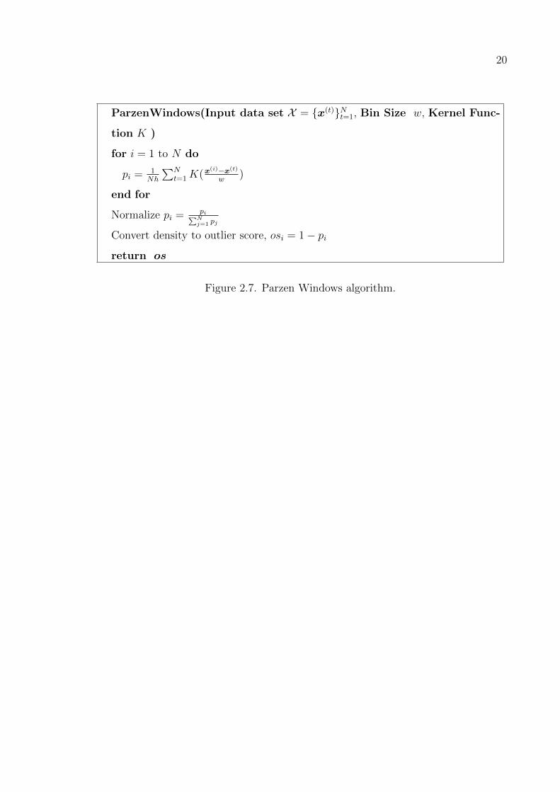
20

ParzenWindows(Input data set X = {x(t)}Nt=1, Bin Size w, Kernel Func-

tion K )

for i = 1 to N do

pi = 1Nh

∑Nt=1K(x

(i)−x(t)

w)

end for

Normalize pi = pi∑Nj=1 pj

Convert density to outlier score, osi = 1− pireturn os

Figure 2.7. Parzen Windows algorithm.

21

3. SPECTRAL METHODS

Spectral methods are unsupervised learning techniques that reveal low dimen-

sional structure in dimensional data [34]. These methods use the spectral decomposi-

tion of specially constructed matrices to reduce dimensionality and transform the input

data to a new space.

We define the following problem. Let us assume that we have N × d data matrix

X = [x(t)]Nt=1 where x(t) ∈ Rd. We want to reach a lower dimensional representation

ZN×m for the N instances such that z(t) ∈ Rm where m < d. We assume, without loss

of generality, that X is centered, i.e.,∑

t x(t) = 0.

Spectral methods find Z by first constructing a similarity matrix S or distance

matrix E. Let us say that we have a similarity matrix S. Then, its spectral decompo-

sition S = WΛWT is calculated, where W is a N × d matrix whose columns are the

eigenvectors of S and Λ is a d× d diagonal matrix whose entries are the corresponding

eigenvalues. Assuming that eigenvalues are sorted in ascending order, we take the last

m eigenvectors from W to be our transformed data Z for dimensionality reduction. If

we use a distance matrix, we take the first m eigenvectors. Before reviewing various

spectral methods, we analyze this generic algorithm in order to understand why this

approach works and what it minimizes as the cost function. We carry out the following

analysis with a similarity matrix S but it is equally valid for a distance matrix since

every distance matrix E can be used as a similarity matrix by setting simply S = −E.

Let us say that we want to find a lower dimensional representation ZN×m for

input data where the dot products in this new space matches the similarities as closely

as possible. In other words, we need to minimize the following cost function:

Cgeneric ≡ ||S− ZZT ||2F = tr[(S− ZZT )T (S− ZZT )] =∑i,j

[(Sij − (z(i))T

(z(j))]2 (3.1)

22

Equation 3.1 is known as low rank matrix approximation problem and its solution is

given by the singular value decomposition of S = UΣVT [35]. Hence, taking the m

left singular vectors with the greatest singular values from V gives Z (in order for

the actual dot product values in the new space to match S values, we need to take

Z = UΣ1/2 but this is not necessary as Σ is only a scaling matrix and does not affect

the transformation). The cost function in Equation 3.1 can also be reformulated as:

∑i,j

(Sij − (z(i))T

(z(j)))2 = tr(SST )− tr(2ZTSZ) + tr(ZZTZZT ) (3.2)

If we add the constraint ZTZ = I to remove the effect of arbitrary scaling and note

that tr(ZZT ) = tr(ZTZ), tr(SST ) is constant and does not depend on Z, minimization

of Equation 3.1 is equivalent to the maximization of

Cgeneric2 ≡ tr(ZTSZ) (3.3)

This is a trace maximization problem and its solution is given by the eigenvectors of

S with the greatest eigenvalues [36]. Therefore, using spectral decomposition of a

similarity matrix corresponds to assuming that the matrix gives the dot products of

instances and we minimize the cost function of Equation 3.1 or maximize the Equation

3.3 to approximate these values in the new space as closely as possible.

3.1. Principal Components Analysis

Principal Components Analysis (PCA) is a well-known dimensionality reduction

method that minimizes the projection error [37]. We have a transformation matrix

Wd×m that is orthonormal WTW = I and our transformed data is Z = XW. We

project Z back to the original space as X = ZWT and then minimize the reconstruction

error:

CPCA ≡ ||X− X||2F = ||X− ZWT ||2F (3.4)

23

By expanding this cost function, we can show that the minimization of the projection

error is equivalent to variance maximization in the transformed space:

||X− ZWT ||2F = tr[(X− ZWT )(X− ZWT )T ]

= tr(XTX−XWZT − ZWTXT + ZWTWZT )

= tr(XTX− ZZT − ZZT + ZZT )

= tr(XTX)− tr(ZTZ)

Therefore, an alternative formulation for the cost function is as follows:

CPCA2 ≡ tr(WTXTXW) (3.5)

Hence, the transformation matrix W that minimizes the projection error and max-

imizes the variance is given by the m greatest eigenvectors of XTX, which is the

covariance matrix when E[X] = 0.

In practice, for very high dimensional and low size samples PCA is carried out

with the Grammian matrix G = XXT instead of the covariance matrix. In that case,

the eigenvectors of G gives directly the transformed data Z because (w is an eigenvector

and λ is its eigenvalue):

(XTX)w = λw (multiply from left with X)

(XX)TXw = λXw

3.2. Kernel Principal Components Analysis

Kernel Principal Components Analysis (KPCA) is a non-linear generalization of

PCA [38]. It is motivated by the desire to apply PCA in the feature space F which

is possibly infinite dimensional and the mapping function φ : Rd → F defines this

nonlinear transformation. If we have a kernel function K : Rd × Rd → R where

24

K(x(i),x(j)) = φ(x(i))Tφ(x(j)), we can apply PCA by taking the eigenvectors as our

transformed points (in that case we do not have an explicit transformation matrix but

only the transformed data):

(φ(X)Tφ(X))w = λw (multiply from left with φ(X))

(φ(X)φ(X)T )φ(X)w = λφ(X)w

Kz = λz

Therefore, the spectral decomposition of K gives us our transformed points, Z. When

φ(x) = x, KPCA reduces to PCA. This is equivalent to using K as our similarity

matrix. Hence, KPCA tries to find a low dimensional representation where dot products

in the new space closely matches the dot products in the feature space. The cost

function minimized by KPCA is:

CKPCA ≡∑i,j

(φ(x(i))Tφ(x(j))− (z(i))

T(z(j)))2 (3.6)

Although, the input data is centered, it may not be in the feature space. However, we

do not have the data in the feature space explicitly, meaning that we cannot simply

calculate the mean and subtract it. Instead, we write φ(x) = φ(x)− (1/N)∑

t φ(x(t))

and K = φ(x)T φ(x) to reach the following normalization to center K where 1N is an

N ×N matrix with (1N)ij := 1/N [39]:

K = K− 1NK−K1N + 1NK1N (3.7)

The mean subtraction step augments the minimized cost function:

CKPCAmc ≡∑i,j

((φ(x(i))− φ(x))T (φ(x(j))− φ(x))− (z(i))T

(z(j)))2 (3.8)

25

3.3. Multidimensional Scaling

Multidimensional Scaling (MDS) is a family of dimensionality reduction methods

with many variants. Here, we discuss the Classical (or Metric) MDS where the aim

is to preserve the Euclidean distances in the projected space as closely as possible

[40]. MDS uses the distance matrix EN×N where Eij is assumed to be the Euclidean

distance between x(i) and x(j): ||x(i)−x(j)||. In order to find the best low dimensional

representation that approximates the pairwise Euclidean distances as well as possible,

the dot product matrix B = XXT is obtained from E [1]:

B = −1

2(E− 1NE− E1N + 1NE1N) (3.9)

We use the spectral decomposition of B to get our transformed data Z by taking the

desired number of eigenvectors of B starting from the ones with the greatest eigenvalues

again. It is clear that we are trying to match the dot products of the transformed

instances z to the actual values in B. In addition, since B is obtained from the

Euclidean distance matrix E, the Euclidean distances between the points in the new

space approximate the original distances in E. MDS minimizes the cost function:

CMDS ≡∑i,j

(||x(i) − x(j)||2 − ||z(i) − z(j)||2)2 (3.10)

If E contains the actual Euclidean distances calculated in the original space, MDS is

equivalent to PCA.

3.4. Laplacian Eigenmaps

Laplacian Eigenmaps (LEM) assumes that each input instance denotes a node

in a graph and uses the adjacency matrix as a similarity matrix [41]. Each instance

is connected to only a small number of nearby instances resulting in a sparse adja-

cency matrix. Edges between connected instances Sij are given constant weight or

are weighted by a Gaussian kernel. However, we may use any similarity measure for

26

weighting the edges. LEM solves the following generalized eigenvalue problem to trans-

form the input data where DN×N is the diagonal matrix of column (or row) sums of

S, Dii =∑

j Sij.

(D− S)z = λDz (3.11)

We omit the eigenvector with the eigenvalue 0 and take the desired number of

eigenvectors starting from the ones with smallest eigenvalues to obtain our transformed

data z. It is known that LEM minimizes the following cost function:

CLEM ≡∑i,j

||z(i) − z(j)||2Sij (3.12)

Let us assume that the new z are one dimensional. Then, z is a N × 1 vector where

∑i,j

(z(i) − z(j))2Sij =∑i,j

((x(i))2 + (x(j))2 − 2x(i)x(j))Sij

=∑i

(x(i))2Dii +∑j

(x(j))2Djj − 2∑i,j

x(i)x(j)Sij

= 2zT (D− S)z

Therefore, in order to minimize Equation 3.12, we need to minimize zT (D− S)z. We

add the constraint zTDz = 1 to remove the effect of arbitrary scaling in the solution.

This optimization problem is solved by the generalized eigenvalue problem given in

Equation 3.11.

3.5. Discussion

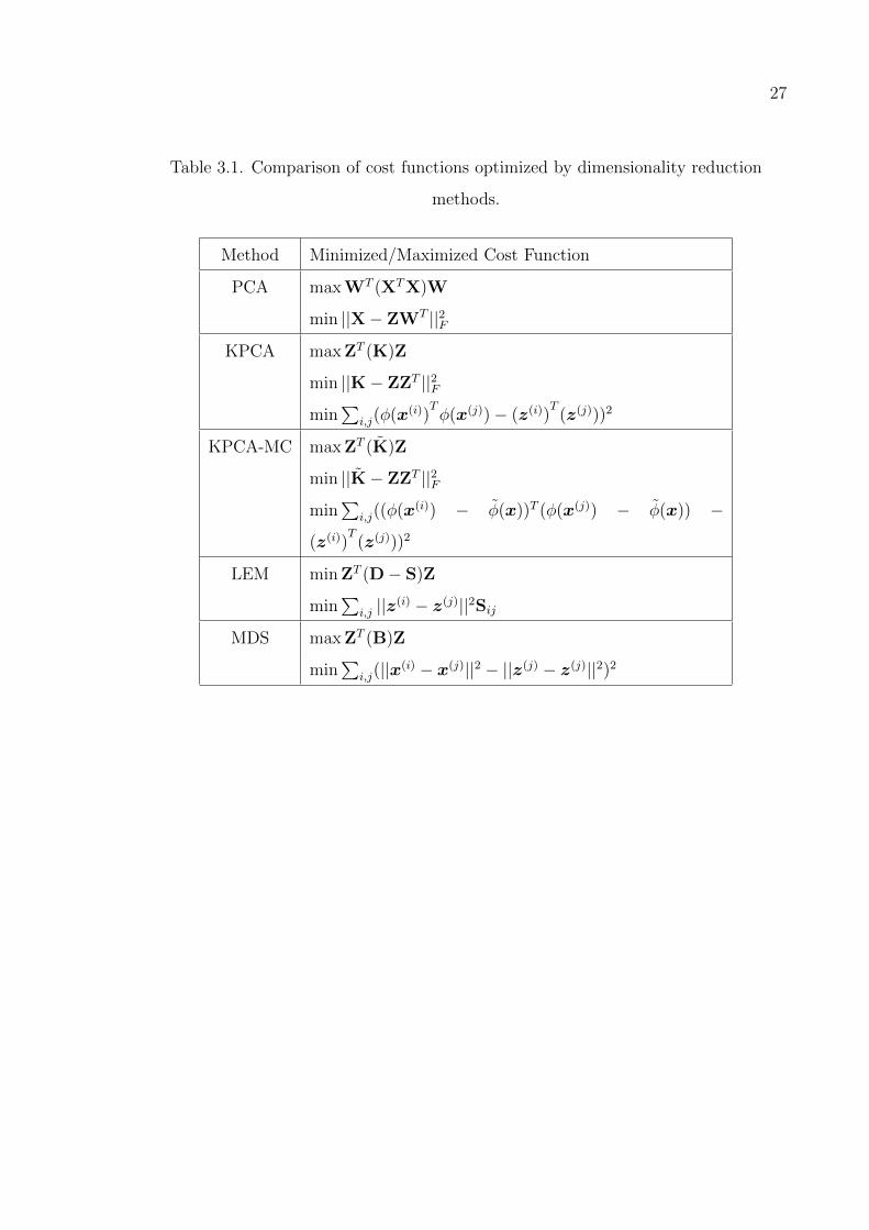
In Table 3.1, we list the cost functions minimized/maximized by the dimensional-

ity reduction methods. We assume that the reduced number of dimensions is 1, m = 1,

in order to get rid of trace operators for the sake of simplicity.

27

Table 3.1. Comparison of cost functions optimized by dimensionality reduction

methods.

Method Minimized/Maximized Cost Function

PCA max WT (XTX)W

min ||X− ZWT ||2FKPCA max ZT (K)Z

min ||K− ZZT ||2Fmin

∑i,j(φ(x(i))

Tφ(x(j))− (z(i))

T(z(j)))2

KPCA-MC max ZT (K)Z

min ||K− ZZT ||2Fmin

∑i,j((φ(x(i)) − φ(x))T (φ(x(j)) − φ(x)) −

(z(i))T

(z(j)))2

LEM min ZT (D− S)Z

min∑

i,j ||z(i) − z(j)||2SijMDS max ZT (B)Z

min∑

i,j(||x(i) − x(j)||2 − ||z(j) − z(j)||2)2

28

−1 −0.5 0 0.5 1−1

−0.5

0

0.5

1Original Data

1 2 3 4 5

−1 −0.5 0 0.5 1−1

−0.5

0

0.5

1PCA

Var=1.000

Var

=0.

000

12345

−1 −0.5 0 0.5 1−1

−0.5

0

0.5

1Laplacian EM

Var=0.316

Var

=0.

490

1

2 3 4

5

−1 −0.5 0 0.5 1−1

−0.5

0

0.5

1Classical MDS

Var=0.652

Var

=0.

501

1

2 3 4

5

−1 −0.5 0 0.5 1−1

−0.5

0

0.5

1KPCA

Var=2.843

Var

=1.

159

1

2

3

4

5

−1 −0.5 0 0.5 1−1

−0.5

0

0.5

1KPCA − Mean Centered

Var=1.228

Var

=1.

159

1

2

3

4

5

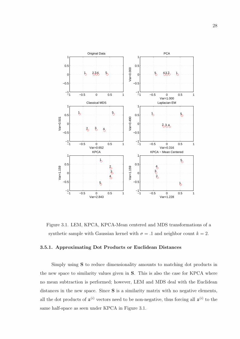
Figure 3.1. LEM, KPCA, KPCA-Mean centered and MDS transformations of a

synthetic sample with Gaussian kernel with σ = .1 and neighbor count k = 2.

3.5.1. Approximating Dot Products or Euclidean Distances

Simply using S to reduce dimensionality amounts to matching dot products in

the new space to similarity values given in S. This is also the case for KPCA where

no mean subtraction is performed; however, LEM and MDS deal with the Euclidean

distances in the new space. Since S is a similarity matrix with no negative elements,

all the dot products of z(i) vectors need to be non-negative, thus forcing all z(i) to the

same half-space as seen under KPCA in Figure 3.1.

29

3.5.2. Mean Centered KPCA is Equivalent to Classical MDS

It is apparent that the mean subtraction step in KPCA is identical to the extrac-

tion of dot products from the Euclidean matrix E. Similarity matrix S can be used as

a distance matrix as E = −S, then mean-centered KPCA is identical to MDS. There-

fore, we can claim that mean subtraction modifies the cost function to approximate

Euclidean distances instead of dot products. A similar transition to the Euclidean

distances from the dot products is achieved in LEM by using D− S matrix. Whereas

using spectral decomposition of S approximates dot products, LEM minimizes the cost

function in Equation 3.12 involving Euclidean distances by using D− S matrix.

3.5.3. How LEM Differs from MDS and KPCA

The cost function minimized by MDS shows us that it approximates the distances

in the original space with the Euclidean distances in the new space. LEM’s cost function

is different in the sense that it weights the Euclidean distances with similarity values

paying more attention to keeping highly similar points close in the new space. For

example in Figure 3.1, three points in the middle, which are more similar to each

other, are mapped to relatively closer points by LEM, while this is not the case for

MDS.

30

4. SPECTRAL OUTLIER DETECTION

4.1. The Idea

In this chapter, we propose our spectral outlier detection method that combines

spectral decomposition with outlier detection. We argue that applying spectral decom-

position on input data before outlier detection has various advantages.

Methods that rely on distances between instances, for instance, density estimation

techniques for outlier detection such as LOF or Parzen Windows, perform poorly as the

number of dimensions increases. The amount of instances that fall into a fixed size bin

decreases dramatically as the dimensionality increases, thus, making it impossible to

estimate a smooth density. Furthermore, distance functions lose their meaning in high

dimensions since pairwise distances tend to be similar for all instances. Although not

as vulnerable as density estimation methods, discriminative methods suffer from high

dimensionality too. For instance, suppose that our method learns a tight boundary, like

in Active-Outlier, then, it is possible to learn a tighter boundary in a lower dimensional

space if data can be projected to lower dimensions with minimal loss of information.

Moreover, processing a higher dimensional data requires more computation. Hence,

reducing input dimensionality with a spectral method alleviates the effect of the curse

of dimensionality and possibly improves outlier detection performance.

Spectral methods find low dimensional structures in data and transform possibly

complicated patterns to smoother ones, therefore, making it possible for discriminative

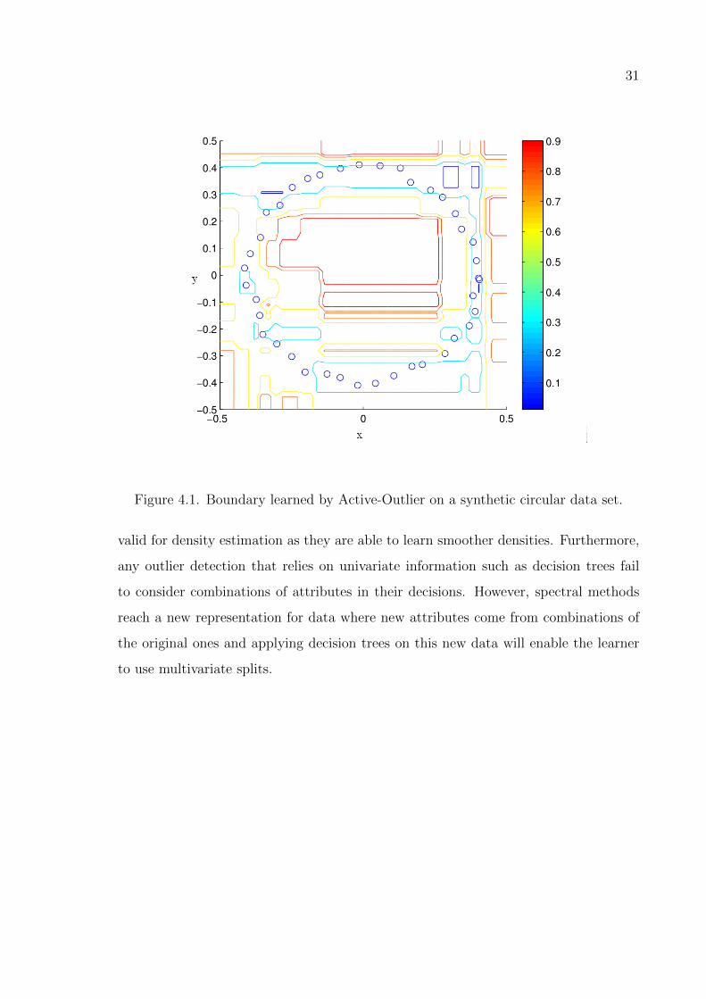
methods to fit simpler boundaries. In Figure 4.1, a circular data set is seen along with

the boundaries learned by the Active-Outlier method. Different contours correspond

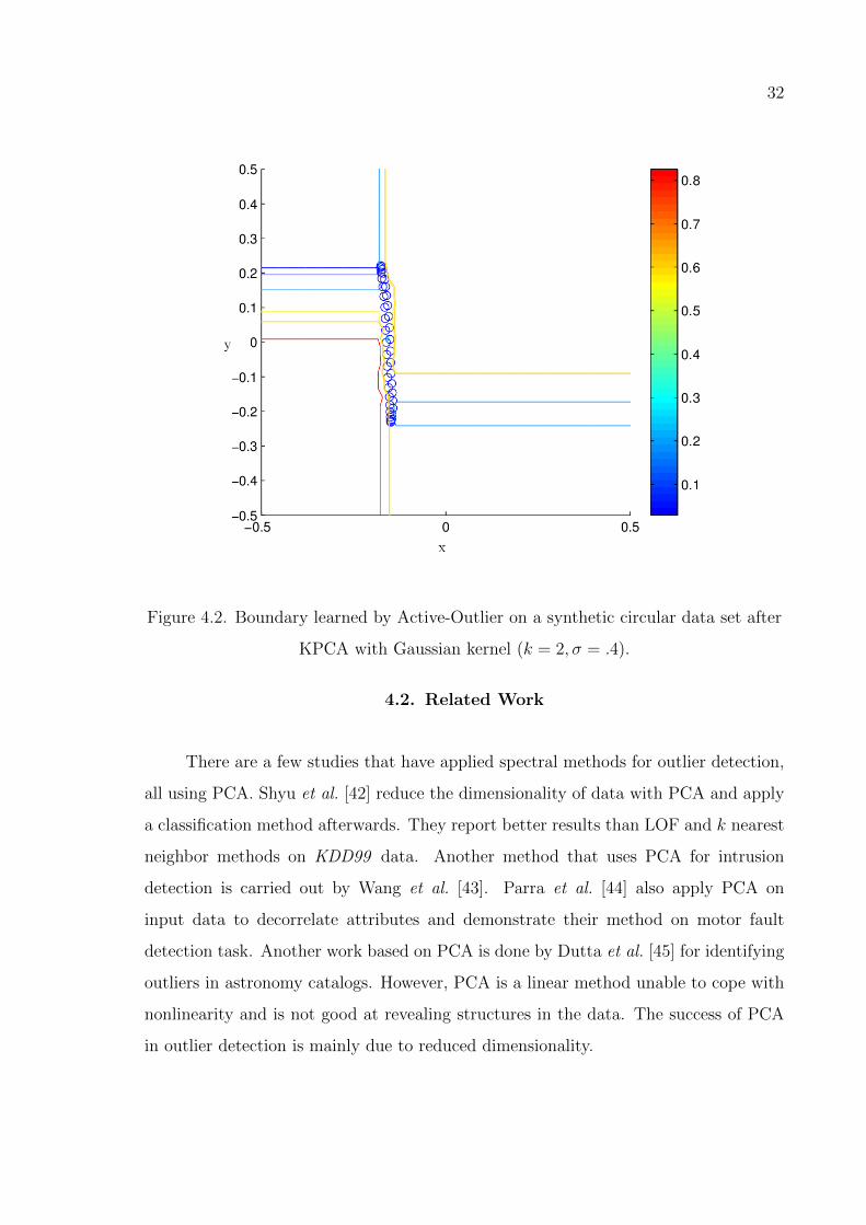
to boundaries for a different threshold value Θ. After applying KPCA on this data set,

we obtain the boundaries seen in Figure 4.2. It is clear that the nonlinear to linear

transformation achieved by the spectral method makes it possible for Active-Outlier

method to learn much simpler boundaries. This advantage of spectral methods is also

31

Figure 4.1. Boundary learned by Active-Outlier on a synthetic circular data set.

valid for density estimation as they are able to learn smoother densities. Furthermore,

any outlier detection that relies on univariate information such as decision trees fail

to consider combinations of attributes in their decisions. However, spectral methods

reach a new representation for data where new attributes come from combinations of

the original ones and applying decision trees on this new data will enable the learner

to use multivariate splits.

32

Figure 4.2. Boundary learned by Active-Outlier on a synthetic circular data set after

KPCA with Gaussian kernel (k = 2, σ = .4).

4.2. Related Work

There are a few studies that have applied spectral methods for outlier detection,

all using PCA. Shyu et al. [42] reduce the dimensionality of data with PCA and apply

a classification method afterwards. They report better results than LOF and k nearest

neighbor methods on KDD99 data. Another method that uses PCA for intrusion

detection is carried out by Wang et al. [43]. Parra et al. [44] also apply PCA on

input data to decorrelate attributes and demonstrate their method on motor fault

detection task. Another work based on PCA is done by Dutta et al. [45] for identifying

outliers in astronomy catalogs. However, PCA is a linear method unable to cope with

nonlinearity and is not good at revealing structures in the data. The success of PCA

in outlier detection is mainly due to reduced dimensionality.

33

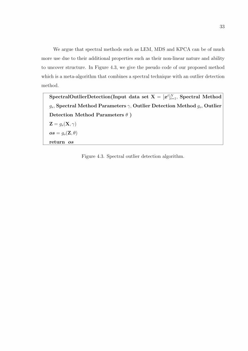
We argue that spectral methods such as LEM, MDS and KPCA can be of much

more use due to their additional properties such as their non-linear nature and ability

to uncover structure. In Figure 4.3, we give the pseudo code of our proposed method

which is a meta-algorithm that combines a spectral technique with an outlier detection

method.

SpectralOutlierDetection(Input data set X = [xt]Nt=1, Spectral Method

gs, Spectral Method Parameters γ, Outlier Detection Method go, Outlier

Detection Method Parameters θ )

Z = gs(X, γ)

os = go(Z, θ)

return os

Figure 4.3. Spectral outlier detection algorithm.

34

5. EXPERIMENTS

Much like the definition of outliers, the evaluation of outlier detection methods is

also a problematic issue. In order to be able to calculate the performance of a method,

it is necessary to have labeled data; however, due to the ambiguity of the outlier

concept, there are various perspectives on evaluating outlier detection methods. In our

experiments, we employ the widely-accepted and well-justified approach of considering

outlier detection as a rare-class classification problem. Assuming that anomalous events

take place much rarely than typical ones, we apply outlier detection methods to real

life scenarios such as network intrusion detection, fault detection, face detection. By

considering the rare classes as outliers, we form multiple data sets and evaluate the

outlier detection methods by their accuracies obtained on these data sets. Apart from

observing accuracies, we also analyze the behavior of the methods on synthetic data

and try to assess these methods visually.

5.1. Evaluated Methods and Implementation Notes

In Active-Outlier (AO) method, we employ C4.5 decision tree [46] as the base

learner and apply no conversion on categorical variables since C4.5 can handle discrete

and numeric attributes together. An important point to note is that in order to reach

high accuracies, learned decision trees should not overfit. Although a decision tree

may be able to classify perfectly a specific data set, such classifiers do not achieve high

accuracies when combined. This problem can be overcome by stopping splitting when

a leaf contains fewer than a certain number of instances; this is known as prepruning.

In our experiments, we observed that limiting the minimum number of instances in a

leaf to bN/16c where N is the sample size leads to good results. For Local Outlier

Factor (LOF) method, due to the high computational requirements of the method, we

have modified it to calculate LOF values for k in the range of kmin to kmax. Instead of

incrementing k from kmin to kmax one by one, we choose a step size s and increment k

by s until we reach kmax. This strategy decreased running time significantly hopefully

35

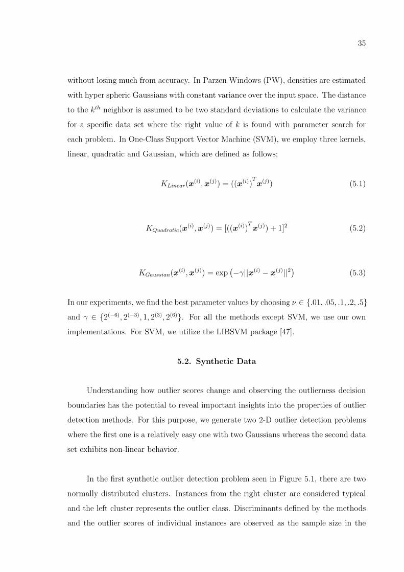
without losing much from accuracy. In Parzen Windows (PW), densities are estimated

with hyper spheric Gaussians with constant variance over the input space. The distance

to the kth neighbor is assumed to be two standard deviations to calculate the variance

for a specific data set where the right value of k is found with parameter search for

each problem. In One-Class Support Vector Machine (SVM), we employ three kernels,

linear, quadratic and Gaussian, which are defined as follows;

KLinear(x(i),x(j)) = ((x(i))

Tx(j)) (5.1)

KQuadratic(x(i),x(j)) = [((x(i))

Tx(j)) + 1]2 (5.2)

KGaussian(x(i),x(j)) = exp(−γ||x(i) − x(j)||2

)(5.3)

In our experiments, we find the best parameter values by choosing ν ∈ {.01, .05, .1, .2, .5}

and γ ∈ {2(−6), 2(−3), 1, 2(3), 2(6)}. For all the methods except SVM, we use our own

implementations. For SVM, we utilize the LIBSVM package [47].

5.2. Synthetic Data

Understanding how outlier scores change and observing the outlierness decision

boundaries has the potential to reveal important insights into the properties of outlier

detection methods. For this purpose, we generate two 2-D outlier detection problems

where the first one is a relatively easy one with two Gaussians whereas the second data

set exhibits non-linear behavior.

In the first synthetic outlier detection problem seen in Figure 5.1, there are two

normally distributed clusters. Instances from the right cluster are considered typical

and the left cluster represents the outlier class. Discriminants defined by the methods

and the outlier scores of individual instances are observed as the sample size in the

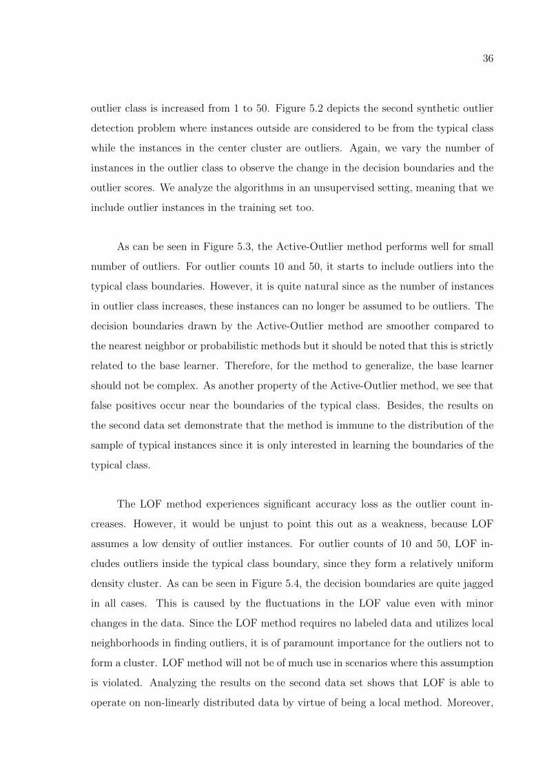
36

outlier class is increased from 1 to 50. Figure 5.2 depicts the second synthetic outlier

detection problem where instances outside are considered to be from the typical class

while the instances in the center cluster are outliers. Again, we vary the number of

instances in the outlier class to observe the change in the decision boundaries and the

outlier scores. We analyze the algorithms in an unsupervised setting, meaning that we

include outlier instances in the training set too.

As can be seen in Figure 5.3, the Active-Outlier method performs well for small

number of outliers. For outlier counts 10 and 50, it starts to include outliers into the

typical class boundaries. However, it is quite natural since as the number of instances

in outlier class increases, these instances can no longer be assumed to be outliers. The

decision boundaries drawn by the Active-Outlier method are smoother compared to

the nearest neighbor or probabilistic methods but it should be noted that this is strictly

related to the base learner. Therefore, for the method to generalize, the base learner

should not be complex. As another property of the Active-Outlier method, we see that

false positives occur near the boundaries of the typical class. Besides, the results on

the second data set demonstrate that the method is immune to the distribution of the

sample of typical instances since it is only interested in learning the boundaries of the

typical class.

The LOF method experiences significant accuracy loss as the outlier count in-

creases. However, it would be unjust to point this out as a weakness, because LOF

assumes a low density of outlier instances. For outlier counts of 10 and 50, LOF in-

cludes outliers inside the typical class boundary, since they form a relatively uniform

density cluster. As can be seen in Figure 5.4, the decision boundaries are quite jagged

in all cases. This is caused by the fluctuations in the LOF value even with minor

changes in the data. Since the LOF method requires no labeled data and utilizes local

neighborhoods in finding outliers, it is of paramount importance for the outliers not to

form a cluster. LOF method will not be of much use in scenarios where this assumption

is violated. Analyzing the results on the second data set shows that LOF is able to

operate on non-linearly distributed data by virtue of being a local method. Moreover,

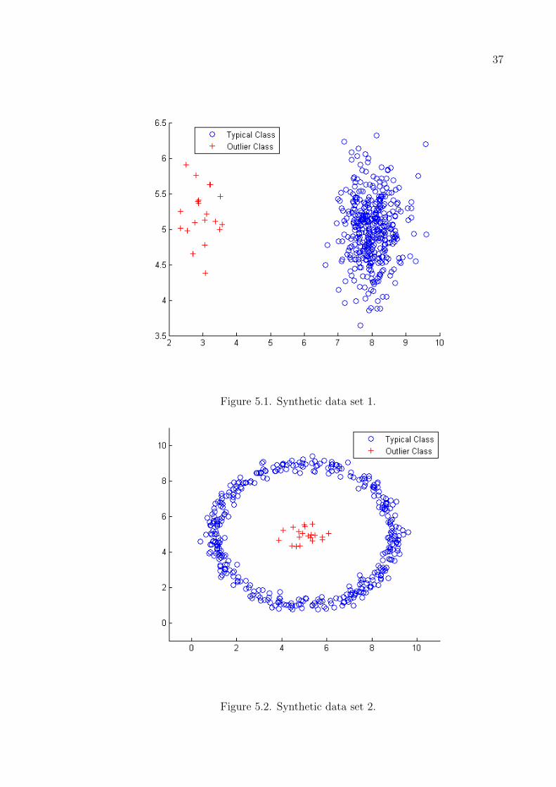
37

Figure 5.1. Synthetic data set 1.

Figure 5.2. Synthetic data set 2.

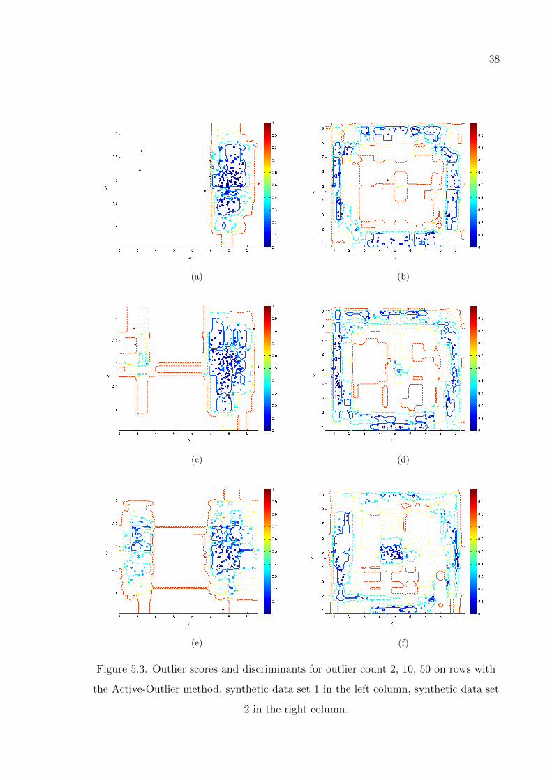
38

(a) (b)

(c) (d)

(e) (f)

Figure 5.3. Outlier scores and discriminants for outlier count 2, 10, 50 on rows with

the Active-Outlier method, synthetic data set 1 in the left column, synthetic data set

2 in the right column.

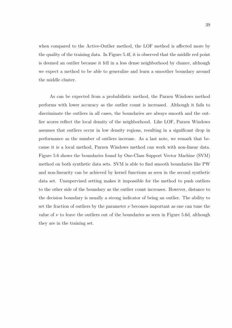
39

when compared to the Active-Outlier method, the LOF method is affected more by

the quality of the training data. In Figure 5.4f, it is observed that the middle red point

is deemed an outlier because it fell in a less dense neighborhood by chance, although

we expect a method to be able to generalize and learn a smoother boundary around

the middle cluster.

As can be expected from a probabilistic method, the Parzen Windows method

performs with lower accuracy as the outlier count is increased. Although it fails to

discriminate the outliers in all cases, the boundaries are always smooth and the out-

lier scores reflect the local density of the neighborhood. Like LOF, Parzen Windows

assumes that outliers occur in low density regions, resulting in a significant drop in

performance as the number of outliers increase. As a last note, we remark that be-

cause it is a local method, Parzen Windows method can work with non-linear data.

Figure 5.6 shows the boundaries found by One-Class Support Vector Machine (SVM)

method on both synthetic data sets. SVM is able to find smooth boundaries like PW

and non-linearity can be achieved by kernel functions as seen in the second synthetic

data set. Unsupervised setting makes it impossible for the method to push outliers

to the other side of the boundary as the outlier count increases. However, distance to

the decision boundary is usually a strong indicator of being an outlier. The ability to

set the fraction of outliers by the parameter ν becomes important as one can tune the

value of ν to leave the outliers out of the boundaries as seen in Figure 5.6d, although

they are in the training set.

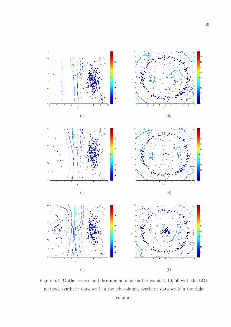
40

(a) (b)

(c) (d)

(e) (f)

Figure 5.4. Outlier scores and discriminants for outlier count 2, 10, 50 with the LOF

method, synthetic data set 1 in the left column, synthetic data set 2 in the right

column.

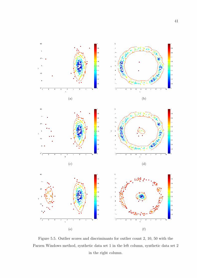
41

(a) (b)

(c) (d)

(e) (f)

Figure 5.5. Outlier scores and discriminants for outlier count 2, 10, 50 with the

Parzen Windows method, synthetic data set 1 in the left column, synthetic data set 2

in the right column.

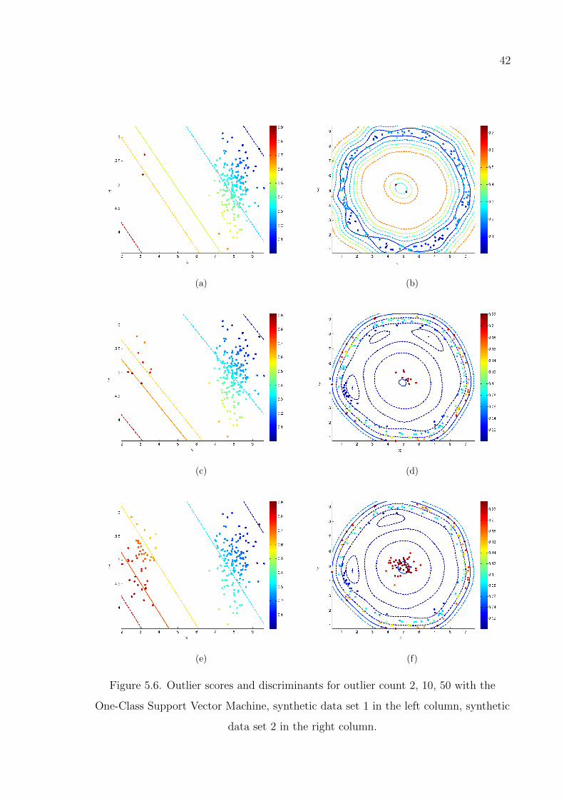
42

(a) (b)

(c) (d)

(e) (f)

Figure 5.6. Outlier scores and discriminants for outlier count 2, 10, 50 with the

One-Class Support Vector Machine, synthetic data set 1 in the left column, synthetic

data set 2 in the right column.

43

5.3. Real Data

We evaluate the performances of Active-Outlier (AO), Local Outlier Factor (LOF),

One-Class SVM (SVM) and Parzen Windows (PW) methods individually and com-

bined with spectral methods on various real data sets. Since we approach the outlier

detection problem from a rare-class classification perspective, we can use the classifica-

tion accuracy as the performance measure. However, in settings where the class priors

are heavily unbalanced, it is much more rational to evaluate methods with measures

invariant under class priors. For this reason, we choose to use the area under the re-

ceiver operating characteristics (AUC) curve [1].

We use 2/3 of each data set as the training/validation set and the rest as the test

set. We carry out a parameter search on the training/validation set to obtain the opti-

mum values of the parameters specific to each method. We obtain 10 AUC values per

data set for each method by applying 5×2 cross validation (CV) on training/validation

sets and report the performance on the test set with the optimum parameters. We

carry out two sets of experiments. For the unsupervised case, the training/validation

set contains both the typical and the outlier sample and in the semi-supervised case,

only the typical sample forms the training/validation set meaning that there are no

outlier instances in the data set.

In our spectral detection algorithm, we combine each of the above methods with

PCA, Laplacian Eigenmaps (LEM) and Multidimensional Scaling (MDS). We apply

PCA on the covariance of the centered input data. LEM requires a similarity matrix

W calculated from the input data. Wij denotes the similarity between inputs x(i)

and x(j). For each instance, we calculate its similarity to its k neighbors and for the

instances not in its k-neighborhood, Wij is set to 0. In our experiments, we use three

different kernels; constant, Gaussian and quadratic polynomial:

KConstant(x(i),x(j)) = 1 (5.4)

44

KGaussian(x(i),x(j)) = exp

(−||x

(i) − x(j)||2

2σ2

)(5.5)

KQuadratic(x(i),x(j)) = [((x(i))

Tx(j)) + 1]2 (5.6)

The variance for the Gaussian kernel, σ, is set to s, half of the average of distances

to kth neighbors. The constant and quadratic kernels require no extra parameters.

For MDS, we convert the similarity matrix W to a distance matrix by negating it,

E = −W. In our experiments, for the neighbor count, k, we try 3, 6, 12, 25 and 80.

We also vary σ value to s/2, 2s and 4s. In PCA, for the number of dimensions in

the transformed space, we try the values that explain 80%, 90%, 95% and 99% of the

variance. For LEM and MDS, we choose four values linearly spaced in the interval

[2, d] where d is the input dimensionality.

5.3.1. Data Sets

The attributes of the data sets used are summarized in Table 5.1.

• Shuttle data set is a low dimensional and large data set collected from the oper-

ation of a shuttle. Approximately 80% of data belongs to the typical class while

the five rare classes have very few instances. We create an outlier detection prob-

lem from this data set by forming a binary classification problem between class

1 and one of the five rare classes, class 3.

• Optdigits data set contains 1024-dimensional images of handwritten digits from

10 classes [48]. We form a problem by taking all the instances from a certain

class as the typical sample and adding a few instances from the other classes as

outliers.

• KDD99 data set [48] is about network intrusion detection and was provided by the

annual International Knowledge Discovery and Data Mining Tools Competition as

a contest problem in 1999. It contains 41 attributes denoting various properties

of network activity and contains labeled network intrusions. Although there

45

are many intrusion classes, the smallest intrusion class, u2r, is chosen as the

outlier class following the general approach in previous publications. The data

set contains separate training and test splits which are known to come from

different distributions. For this reason, we apply the outlier detection methods

on two separate data sets; KDD99Train and KDD99Test.

• Pageblocks data set consists of 10 dimensional instances containing features ex-

tracted from blocks of the page layout of several documents. There are four

classes; text, horizontal line, vertical line, picture and graphic. Nearly 90% of

documents belong to the text class which is considered as the typical sample. We

again discriminate between the typical class and one of the rare classes.

• Abalone data set contains physical measurements of abalones and the task is to

predict the age. We take the class with the most instances to be the typical class

and add a low sample sized class as outliers.

• In Glass data set, the properties of glasses are used to discriminate between

different types. We take window glasses as the typical class and combine the

others as the outliers.

• Yeast data set contains various properties of protein sequences and the class labels

indicate their localization sites. Cytosolic sequences are considered to be typical

whereas peroxisomal ones are the outliers.

• Cardiotocography data set consists of fetal cardiotocograms (CTG) where experts

classified CTGs both with respect to the morphological pattern and the fetal

state. We use the fetal state classification and try to discriminate between normal

and pathologic instances.

• Spam data set contains various word and character frequency related attributes of

e-mails from a large corpora and their labels. We assume that non-spam e-mails

are typical and the spams are the outliers.

• Ecoli data set is very similar to Yeast, also concerning the localization sites of

proteins. The class with the most instances is the typical one while the outer

membrane proteins are considered to be the outliers.

• Letter data set is made up of the numerical attributes of the letters in the English

alphabet obtained from black and white letter images. We choose one letter to

46

be typical and add a few instances from others to form the outlier class.

• Satellite data set consists of the multi-spectral values of pixels in 3 × 3 neigh-

bourhoods in a satellite image and the classification of the region with respect to

soil type. We take the largest class to be the typical one and one of the others as

the outlier.

• Wine data set contains various attributes concerning the chemical properties of

wines and each wine is classified with respect to its quality. We consider the

medium quality to be typical and add poor quality instances as outliers.

• Breast and Mammography are cancer diagnosis data sets containing features ex-

tracted from images of breast masses and medical tests. We take the benign

instances as the typical class and add the malignant instances as outliers.

• In Pima data set, patient information is used to decide whether the patient shows

signs of diabetes. Healthy patients are considered typical and patients diagnosed

with diabetes are the outliers.

• Robot data set contains force and torque measurements on a robot after fail-

ure detection in five different learning problems. We form the outlier detection

problem by taking the normal instances from all problems against the collision

instances from the first problem.

• Vehicle data set consists of shape features extracted from vehicle silhouettes and

their classification into four classes. We group three classes into one and use it

as the typical class where the bus class is the outlier class because it is relatively

different than the other classes.

• Secom data set deals with fault detection in a semi-conductor manufacturing

process. The features are gathered from sensors and each product is classified as

pass or fail. We consider the faulty products to be outliers.

Whereas the Active-Outlier method can operate directly on categorical features,

for other methods, we convert these features to continuous ones by replacing them with

inverse document frequencies and in order to prevent the effect of different scales on

methods relying on distances, data are normalized to the [0, 1] interval.

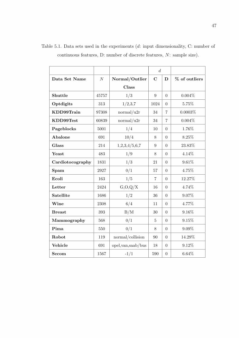
47

Table 5.1. Data sets used in the experiments (d: input dimensionality, C: number of

continuous features, D: number of discrete features, N : sample size).

d

Data Set Name N Normal/Outlier

Class

C D % of outliers

Shuttle 45757 1/3 9 0 0.004%

Optdigits 313 1/2,3,7 1024 0 5.75%

KDD99Train 97308 normal/u2r 34 7 0.0003%

KDD99Test 60839 normal/u2r 34 7 0.004%

Pageblocks 5001 1/4 10 0 1.76%

Abalone 691 10/4 8 0 8.25%

Glass 214 1,2,3,4/5,6,7 9 0 23.83%

Yeast 483 1/9 8 0 4.14%

Cardiotocography 1831 1/3 21 0 9.61%

Spam 2927 0/1 57 0 4.75%

Ecoli 163 1/5 7 0 12.27%

Letter 2424 G,O,Q/X 16 0 4.74%

Satellite 1686 1/2 36 0 9.07%

Wine 2308 6/4 11 0 4.77%

Breast 393 B/M 30 0 9.16%

Mammography 568 0/1 5 0 9.15%

Pima 550 0/1 8 0 9.09%

Robot 119 normal/collision 90 0 14.29%

Vehicle 691 opel,van,saab/bus 18 0 9.12%

Secom 1567 -1/1 590 0 6.64%

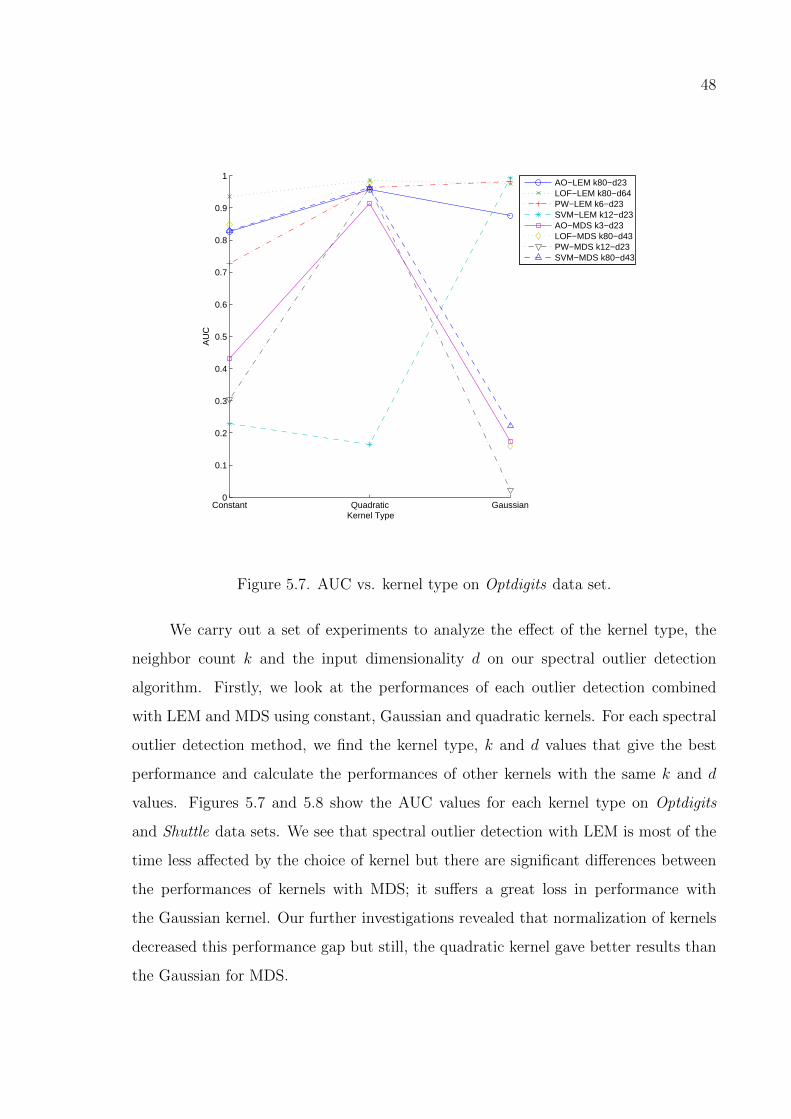
48

Constant Quadratic Gaussian0

0.1

0.2

0.3

0.4

0.5

0.6

0.7

0.8

0.9

1

Kernel Type

AU

C

AO−LEM k80−d23LOF−LEM k80−d64PW−LEM k6−d23SVM−LEM k12−d23AO−MDS k3−d23LOF−MDS k80−d43PW−MDS k12−d23SVM−MDS k80−d43

Figure 5.7. AUC vs. kernel type on Optdigits data set.

We carry out a set of experiments to analyze the effect of the kernel type, the

neighbor count k and the input dimensionality d on our spectral outlier detection

algorithm. Firstly, we look at the performances of each outlier detection combined

with LEM and MDS using constant, Gaussian and quadratic kernels. For each spectral

outlier detection method, we find the kernel type, k and d values that give the best

performance and calculate the performances of other kernels with the same k and d

values. Figures 5.7 and 5.8 show the AUC values for each kernel type on Optdigits

and Shuttle data sets. We see that spectral outlier detection with LEM is most of the

time less affected by the choice of kernel but there are significant differences between

the performances of kernels with MDS; it suffers a great loss in performance with

the Gaussian kernel. Our further investigations revealed that normalization of kernels

decreased this performance gap but still, the quadratic kernel gave better results than

the Gaussian for MDS.

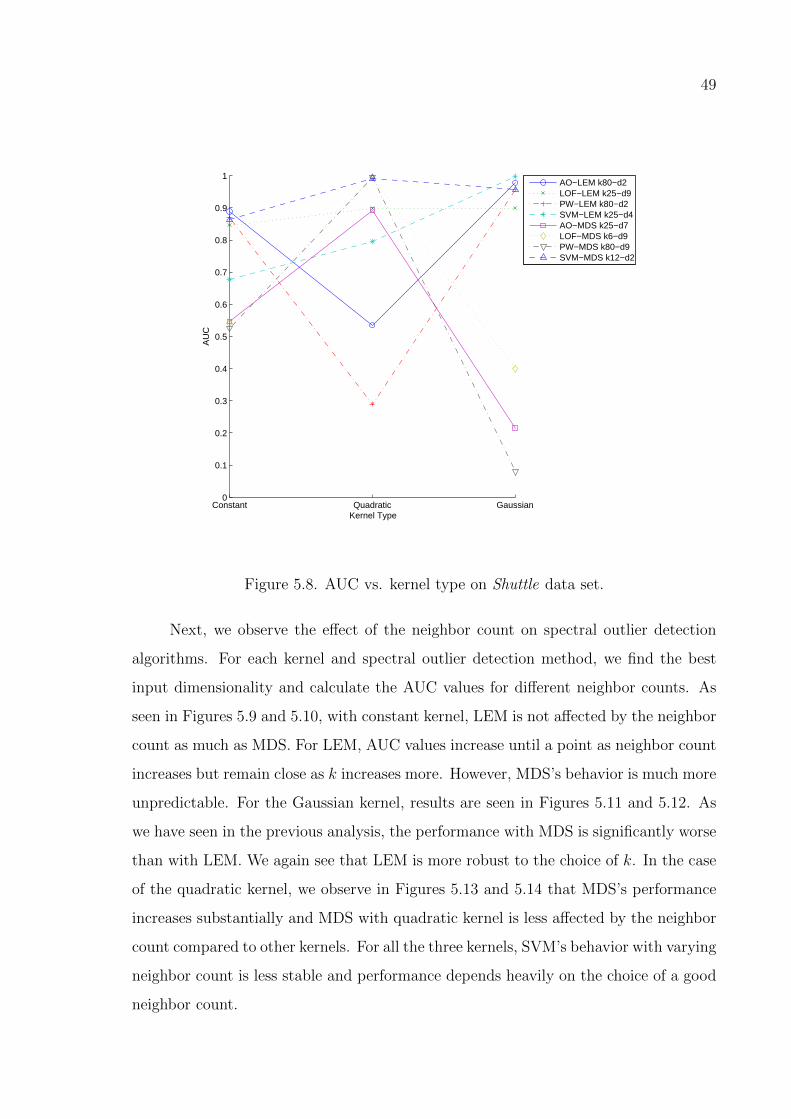
49

Constant Quadratic Gaussian0

0.1

0.2

0.3

0.4

0.5

0.6

0.7

0.8

0.9

1

Kernel Type

AU

C

AO−LEM k80−d2LOF−LEM k25−d9PW−LEM k80−d2SVM−LEM k25−d4AO−MDS k25−d7LOF−MDS k6−d9PW−MDS k80−d9SVM−MDS k12−d2

Figure 5.8. AUC vs. kernel type on Shuttle data set.

Next, we observe the effect of the neighbor count on spectral outlier detection

algorithms. For each kernel and spectral outlier detection method, we find the best

input dimensionality and calculate the AUC values for different neighbor counts. As

seen in Figures 5.9 and 5.10, with constant kernel, LEM is not affected by the neighbor

count as much as MDS. For LEM, AUC values increase until a point as neighbor count

increases but remain close as k increases more. However, MDS’s behavior is much more

unpredictable. For the Gaussian kernel, results are seen in Figures 5.11 and 5.12. As

we have seen in the previous analysis, the performance with MDS is significantly worse

than with LEM. We again see that LEM is more robust to the choice of k. In the case

of the quadratic kernel, we observe in Figures 5.13 and 5.14 that MDS’s performance

increases substantially and MDS with quadratic kernel is less affected by the neighbor

count compared to other kernels. For all the three kernels, SVM’s behavior with varying

neighbor count is less stable and performance depends heavily on the choice of a good

neighbor count.

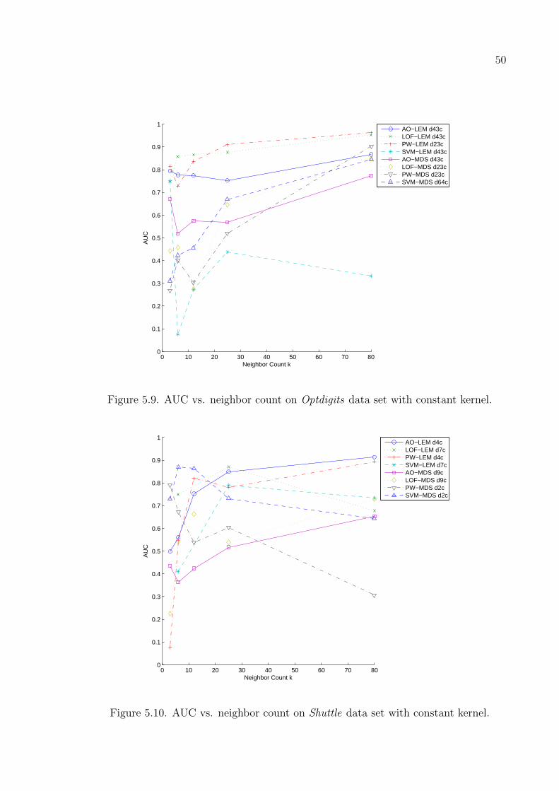
50

0 10 20 30 40 50 60 70 800

0.1

0.2

0.3

0.4

0.5

0.6

0.7

0.8

0.9

1

Neighbor Count k

AU

C

AO−LEM d43cLOF−LEM d43cPW−LEM d23cSVM−LEM d43cAO−MDS d43cLOF−MDS d23cPW−MDS d23cSVM−MDS d64c

Figure 5.9. AUC vs. neighbor count on Optdigits data set with constant kernel.

0 10 20 30 40 50 60 70 800

0.1

0.2

0.3

0.4

0.5

0.6

0.7

0.8

0.9

1

Neighbor Count k

AU

C

AO−LEM d4cLOF−LEM d7cPW−LEM d4cSVM−LEM d7cAO−MDS d9cLOF−MDS d9cPW−MDS d2cSVM−MDS d2c

Figure 5.10. AUC vs. neighbor count on Shuttle data set with constant kernel.

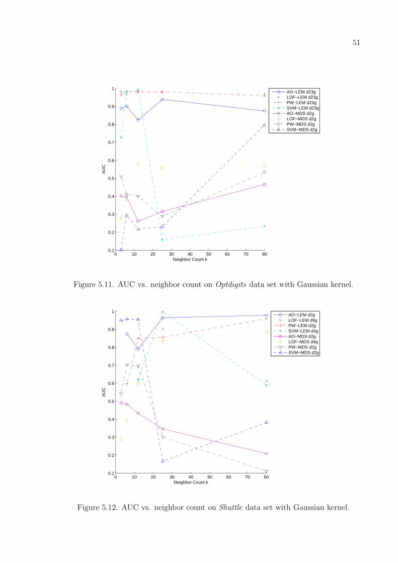
51

0 10 20 30 40 50 60 70 800.1

0.2

0.3

0.4

0.5

0.6

0.7

0.8

0.9

1

Neighbor Count k

AU

C

AO−LEM d23gLOF−LEM d23gPW−LEM d23gSVM−LEM d23gAO−MDS d2gLOF−MDS d2gPW−MDS d2gSVM−MDS d2g

Figure 5.11. AUC vs. neighbor count on Optdigits data set with Gaussian kernel.

0 10 20 30 40 50 60 70 800.1

0.2

0.3

0.4

0.5

0.6

0.7

0.8

0.9

1

Neighbor Count k

AU

C

AO−LEM d2gLOF−LEM d9gPW−LEM d2gSVM−LEM d4gAO−MDS d2gLOF−MDS d4gPW−MDS d2gSVM−MDS d2g

Figure 5.12. AUC vs. neighbor count on Shuttle data set with Gaussian kernel.

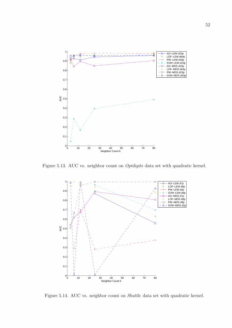
52

0 10 20 30 40 50 60 70 800

0.1

0.2

0.3

0.4

0.5

0.6

0.7

0.8

0.9

1

Neighbor Count k

AU

C

AO−LEM d23pLOF−LEM d64pPW−LEM d43pSVM−LEM d23pAO−MDS d23pLOF−MDS d43pPW−MDS d23pSVM−MDS d43p

Figure 5.13. AUC vs. neighbor count on Optdigits data set with quadratic kernel.

0 10 20 30 40 50 60 70 800

0.1

0.2

0.3

0.4

0.5

0.6

0.7

0.8

0.9

1

Neighbor Count k

AU

C

AO−LEM d7pLOF−LEM d9pPW−LEM d4pSVM−LEM d9pAO−MDS d7pLOF−MDS d9pPW−MDS d9pSVM−MDS d2p

Figure 5.14. AUC vs. neighbor count on Shuttle data set with quadratic kernel.

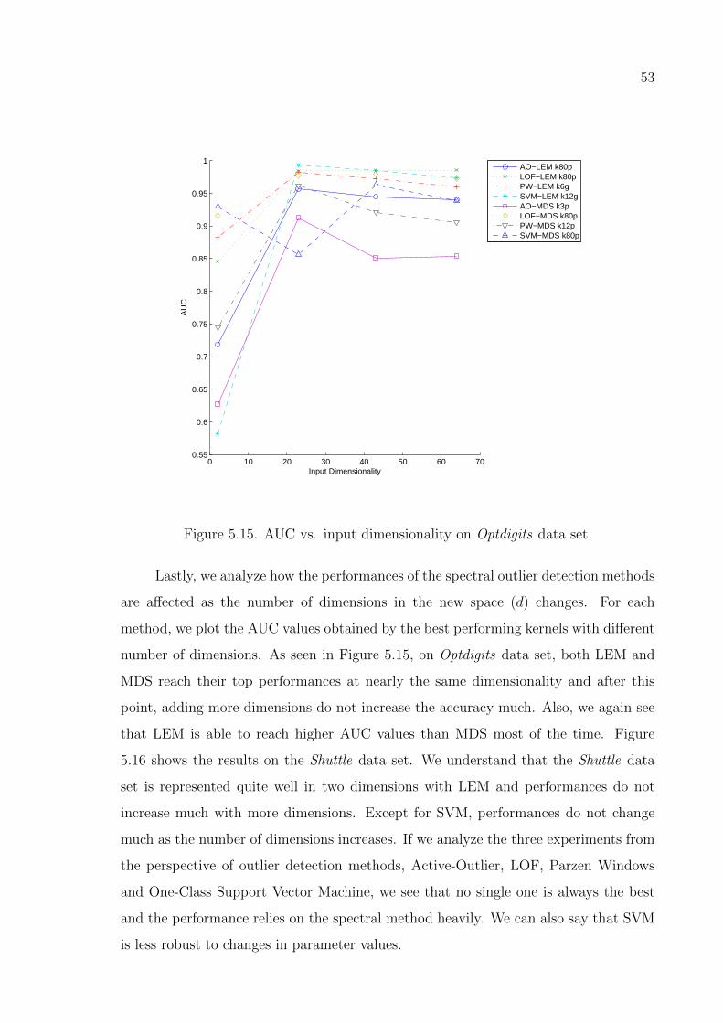
53

0 10 20 30 40 50 60 700.55

0.6

0.65

0.7

0.75

0.8

0.85

0.9

0.95

1

Input Dimensionality

AU

C

AO−LEM k80pLOF−LEM k80pPW−LEM k6gSVM−LEM k12gAO−MDS k3pLOF−MDS k80pPW−MDS k12pSVM−MDS k80p

Figure 5.15. AUC vs. input dimensionality on Optdigits data set.

Lastly, we analyze how the performances of the spectral outlier detection methods

are affected as the number of dimensions in the new space (d) changes. For each

method, we plot the AUC values obtained by the best performing kernels with different

number of dimensions. As seen in Figure 5.15, on Optdigits data set, both LEM and

MDS reach their top performances at nearly the same dimensionality and after this

point, adding more dimensions do not increase the accuracy much. Also, we again see

that LEM is able to reach higher AUC values than MDS most of the time. Figure

5.16 shows the results on the Shuttle data set. We understand that the Shuttle data

set is represented quite well in two dimensions with LEM and performances do not

increase much with more dimensions. Except for SVM, performances do not change

much as the number of dimensions increases. If we analyze the three experiments from

the perspective of outlier detection methods, Active-Outlier, LOF, Parzen Windows

and One-Class Support Vector Machine, we see that no single one is always the best

and the performance relies on the spectral method heavily. We can also say that SVM

is less robust to changes in parameter values.

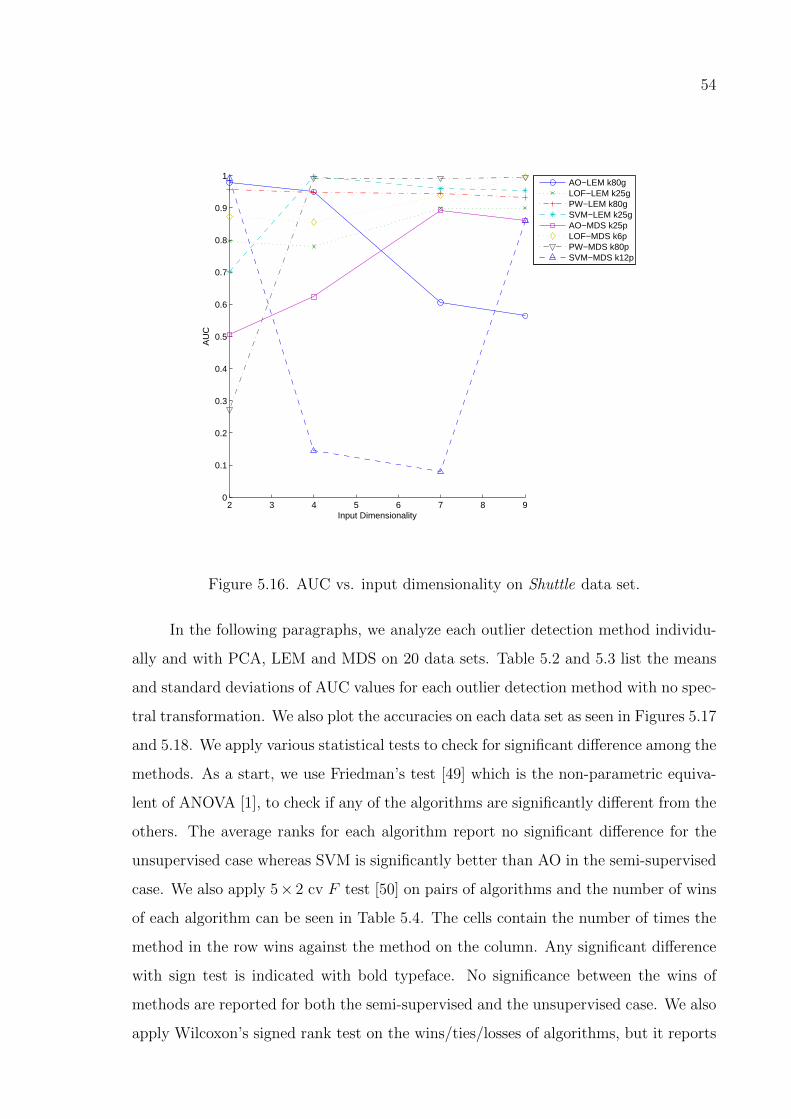
54

2 3 4 5 6 7 8 90

0.1

0.2

0.3

0.4

0.5

0.6

0.7

0.8

0.9

1

Input Dimensionality

AU

C

AO−LEM k80gLOF−LEM k25gPW−LEM k80gSVM−LEM k25gAO−MDS k25pLOF−MDS k6pPW−MDS k80pSVM−MDS k12p

Figure 5.16. AUC vs. input dimensionality on Shuttle data set.

In the following paragraphs, we analyze each outlier detection method individu-

ally and with PCA, LEM and MDS on 20 data sets. Table 5.2 and 5.3 list the means

and standard deviations of AUC values for each outlier detection method with no spec-

tral transformation. We also plot the accuracies on each data set as seen in Figures 5.17

and 5.18. We apply various statistical tests to check for significant difference among the

methods. As a start, we use Friedman’s test [49] which is the non-parametric equiva-

lent of ANOVA [1], to check if any of the algorithms are significantly different from the

others. The average ranks for each algorithm report no significant difference for the

unsupervised case whereas SVM is significantly better than AO in the semi-supervised

case. We also apply 5× 2 cv F test [50] on pairs of algorithms and the number of wins

of each algorithm can be seen in Table 5.4. The cells contain the number of times the

method in the row wins against the method on the column. Any significant difference

with sign test is indicated with bold typeface. No significance between the wins of

methods are reported for both the semi-supervised and the unsupervised case. We also

apply Wilcoxon’s signed rank test on the wins/ties/losses of algorithms, but it reports

55

Table 5.2. Average values and standard deviations of AUCs for the semi-supervised

case.

ActiveOutlier LOF ParzenWindow Svm

shuttle2 1.00±0.0004 0.96±0.010 0.87±0.015 1.00±0.0003

optdigits2 0.93±0.023 0.99±0.006 1.00±0.002 0.99±0.005

kdd99Half 0.91±0.034 0.88±0.009 0.99±0.001 0.99±0.001

kdd99trainHalf 0.99±0.026 0.90±0.023 0.99±0.0003 0.99±0.002

pageblocks3 0.87±0.056 0.93±0.008 0.88±0.016 0.95±0.003

abalone 0.95±0.062 1.00±0.004 1.00±0.001 1.00±0.000

glass 0.89±0.055 0.97±0.009 0.96±0.007 0.98±0.004

yeast 0.60±0.122 0.66±0.023 0.62±0.008 0.71±0.014

cardiotocography 0.62±0.141 0.92±0.012 0.95±0.002 0.97±0.005

spam 0.79±0.064 0.67±0.005 0.74±0.013 0.83±0.003

ecoli 0.96±0.031 0.98±0.011 0.99±0.010 0.99±0.007

letter 0.79±0.050 0.98±0.005 0.87±0.004 0.97±0.005

satellite 1.00±0.001 1.00±0.000 1.00±0.000 1.00±0.000

wine 0.69±0.041 0.76±0.015 0.75±0.006 0.75±0.022

breast 0.89±0.034 0.94±0.015 0.94±0.006 0.93±0.010

mammography 0.72±0.052 0.58±0.048 0.72±0.017 0.70±0.004

pima 0.66±0.022 0.62±0.022 0.78±0.008 0.73±0.028

robot 0.89±0.138 0.99±0.020 0.66±0.046 0.95±0.039

vehicle 0.71±0.059 0.67±0.039 0.57±0.028 0.81±0.030

secom 0.54±0.021 0.58±0.012 0.56±0.009 0.56±0.017

Average Ranks 3.30 2.60 2.35 1.75

no significant differences either. Any significant difference according to Wilcoxon’s test

is marked with an asterisk.

We carry out the same statistical tests to check for differences between the out-

lier detection methods when combined with a spectral method. For PCA, Tables 5.5

and 5.6 list the accuracies and Figures 5.19 and 5.20 show the plots. The number of

dimensions that give the best performance on each data set are given in parentheses.

Friedman’s test reports no significant differences in the semi-supervised case while SVM

is significantly better than LOF in the unsupervised case. Sign test and Wilcoxon’s

signed rank test on the wins of methods, seen in Table 5.7, report no significant differ-

ences except SVM is better than LOF in the unsupervised case according to Wilcoxon’s

signed rank test. The results for LEM can be seen in Tables 5.8, 5.9, 5.10 and Figures

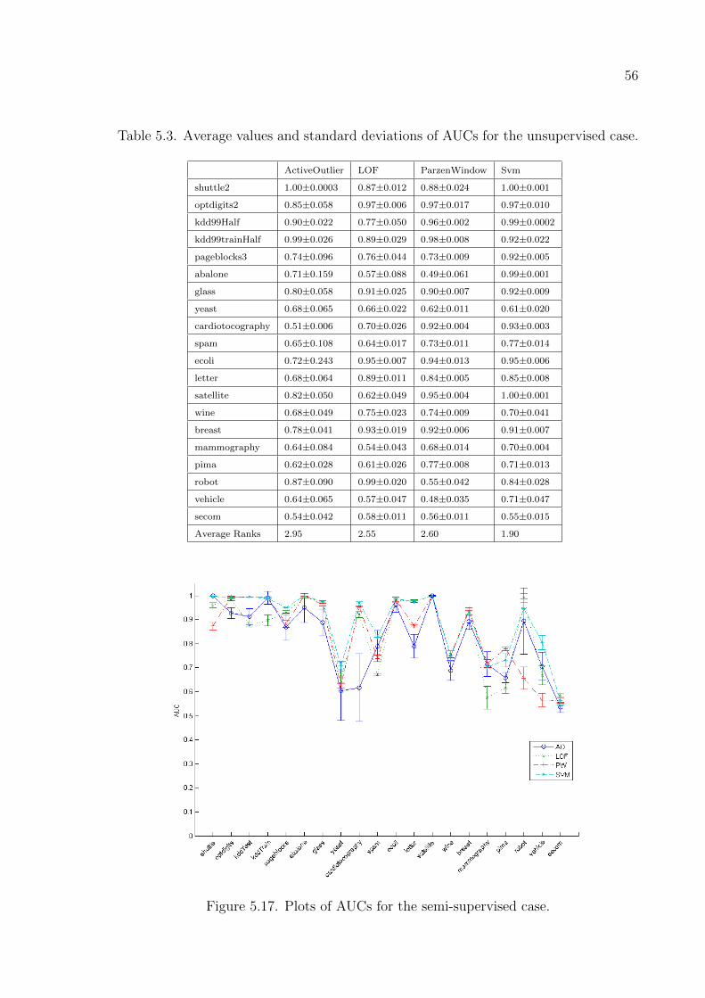
56

Table 5.3. Average values and standard deviations of AUCs for the unsupervised case.

ActiveOutlier LOF ParzenWindow Svm

shuttle2 1.00±0.0003 0.87±0.012 0.88±0.024 1.00±0.001

optdigits2 0.85±0.058 0.97±0.006 0.97±0.017 0.97±0.010

kdd99Half 0.90±0.022 0.77±0.050 0.96±0.002 0.99±0.0002

kdd99trainHalf 0.99±0.026 0.89±0.029 0.98±0.008 0.92±0.022

pageblocks3 0.74±0.096 0.76±0.044 0.73±0.009 0.92±0.005

abalone 0.71±0.159 0.57±0.088 0.49±0.061 0.99±0.001

glass 0.80±0.058 0.91±0.025 0.90±0.007 0.92±0.009

yeast 0.68±0.065 0.66±0.022 0.62±0.011 0.61±0.020

cardiotocography 0.51±0.006 0.70±0.026 0.92±0.004 0.93±0.003

spam 0.65±0.108 0.64±0.017 0.73±0.011 0.77±0.014

ecoli 0.72±0.243 0.95±0.007 0.94±0.013 0.95±0.006

letter 0.68±0.064 0.89±0.011 0.84±0.005 0.85±0.008

satellite 0.82±0.050 0.62±0.049 0.95±0.004 1.00±0.001

wine 0.68±0.049 0.75±0.023 0.74±0.009 0.70±0.041

breast 0.78±0.041 0.93±0.019 0.92±0.006 0.91±0.007

mammography 0.64±0.084 0.54±0.043 0.68±0.014 0.70±0.004

pima 0.62±0.028 0.61±0.026 0.77±0.008 0.71±0.013

robot 0.87±0.090 0.99±0.020 0.55±0.042 0.84±0.028

vehicle 0.64±0.065 0.57±0.047 0.48±0.035 0.71±0.047

secom 0.54±0.042 0.58±0.011 0.56±0.011 0.55±0.015

Average Ranks 2.95 2.55 2.60 1.90

Figure 5.17. Plots of AUCs for the semi-supervised case.

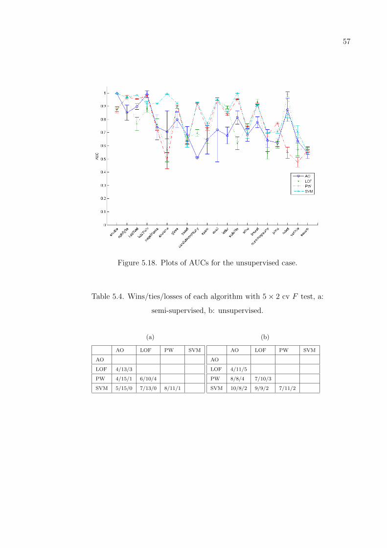
57

Figure 5.18. Plots of AUCs for the unsupervised case.

Table 5.4. Wins/ties/losses of each algorithm with 5× 2 cv F test, a:

semi-supervised, b: unsupervised.

(a)

AO LOF PW SVM

AO

LOF 4/13/3

PW 4/15/1 6/10/4

SVM 5/15/0 7/13/0 8/11/1

(b)

AO LOF PW SVM

AO

LOF 4/11/5

PW 8/8/4 7/10/3

SVM 10/8/2 9/9/2 7/11/2

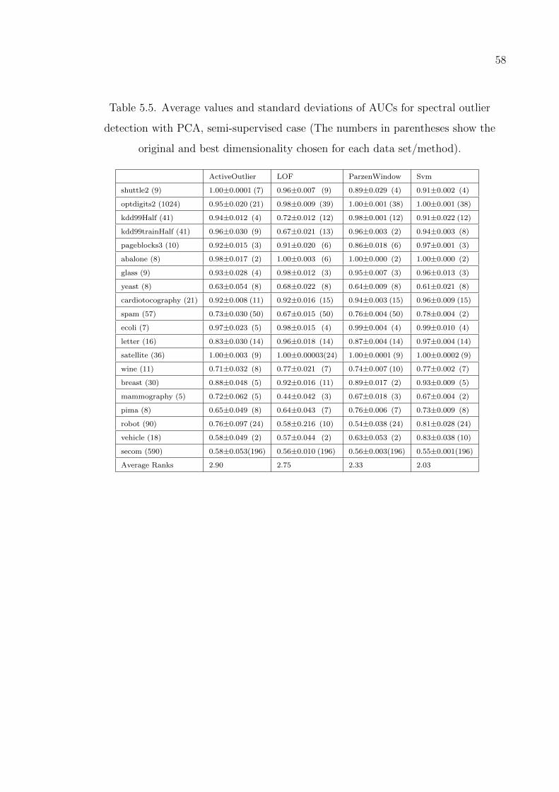
58

Table 5.5. Average values and standard deviations of AUCs for spectral outlier

detection with PCA, semi-supervised case (The numbers in parentheses show the

original and best dimensionality chosen for each data set/method).

ActiveOutlier LOF ParzenWindow Svm

shuttle2 (9) 1.00±0.0001 (7) 0.96±0.007 (9) 0.89±0.029 (4) 0.91±0.002 (4)

optdigits2 (1024) 0.95±0.020 (21) 0.98±0.009 (39) 1.00±0.001 (38) 1.00±0.001 (38)

kdd99Half (41) 0.94±0.012 (4) 0.72±0.012 (12) 0.98±0.001 (12) 0.91±0.022 (12)

kdd99trainHalf (41) 0.96±0.030 (9) 0.67±0.021 (13) 0.96±0.003 (2) 0.94±0.003 (8)

pageblocks3 (10) 0.92±0.015 (3) 0.91±0.020 (6) 0.86±0.018 (6) 0.97±0.001 (3)

abalone (8) 0.98±0.017 (2) 1.00±0.003 (6) 1.00±0.000 (2) 1.00±0.000 (2)

glass (9) 0.93±0.028 (4) 0.98±0.012 (3) 0.95±0.007 (3) 0.96±0.013 (3)

yeast (8) 0.63±0.054 (8) 0.68±0.022 (8) 0.64±0.009 (8) 0.61±0.021 (8)

cardiotocography (21) 0.92±0.008 (11) 0.92±0.016 (15) 0.94±0.003 (15) 0.96±0.009 (15)

spam (57) 0.73±0.030 (50) 0.67±0.015 (50) 0.76±0.004 (50) 0.78±0.004 (2)

ecoli (7) 0.97±0.023 (5) 0.98±0.015 (4) 0.99±0.004 (4) 0.99±0.010 (4)

letter (16) 0.83±0.030 (14) 0.96±0.018 (14) 0.87±0.004 (14) 0.97±0.004 (14)

satellite (36) 1.00±0.003 (9) 1.00±0.00003(24) 1.00±0.0001 (9) 1.00±0.0002 (9)

wine (11) 0.71±0.032 (8) 0.77±0.021 (7) 0.74±0.007 (10) 0.77±0.002 (7)

breast (30) 0.88±0.048 (5) 0.92±0.016 (11) 0.89±0.017 (2) 0.93±0.009 (5)

mammography (5) 0.72±0.062 (5) 0.44±0.042 (3) 0.67±0.018 (3) 0.67±0.004 (2)

pima (8) 0.65±0.049 (8) 0.64±0.043 (7) 0.76±0.006 (7) 0.73±0.009 (8)

robot (90) 0.76±0.097 (24) 0.58±0.216 (10) 0.54±0.038 (24) 0.81±0.028 (24)

vehicle (18) 0.58±0.049 (2) 0.57±0.044 (2) 0.63±0.053 (2) 0.83±0.038 (10)

secom (590) 0.58±0.053(196) 0.56±0.010 (196) 0.56±0.003(196) 0.55±0.001(196)

Average Ranks 2.90 2.75 2.33 2.03

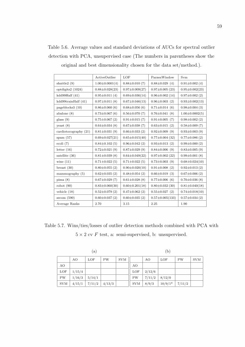
59

Table 5.6. Average values and standard deviations of AUCs for spectral outlier

detection with PCA, unsupervised case (The numbers in parentheses show the

original and best dimensionality chosen for the data set/method.).

ActiveOutlier LOF ParzenWindow Svm

shuttle2 (9) 1.00±0.0001(4) 0.88±0.010 (7) 0.88±0.029 (4) 0.91±0.002 (4)

optdigits2 (1024) 0.88±0.028(23) 0.97±0.009(27) 0.97±0.005 (23) 0.95±0.002(23)

kdd99Half (41) 0.95±0.011 (4) 0.69±0.036(14) 0.96±0.002 (14) 0.97±0.002 (2)

kdd99trainHalf (41) 0.97±0.011 (8) 0.67±0.046(13) 0.96±0.003 (2) 0.93±0.002(13)

pageblocks3 (10) 0.86±0.060 (6) 0.68±0.056 (6) 0.71±0.014 (6) 0.98±0.004 (3)

abalone (8) 0.73±0.067 (6) 0.56±0.070 (7) 0.76±0.041 (8) 1.00±0.0002(5)

glass (9) 0.75±0.067 (2) 0.91±0.015 (7) 0.91±0.005 (7) 0.98±0.002 (2)

yeast (8) 0.64±0.034 (8) 0.67±0.038 (7) 0.63±0.015 (2) 0.58±0.009 (7)

cardiotocography (21) 0.81±0.031 (9) 0.66±0.033 (2) 0.92±0.009 (9) 0.93±0.003 (9)

spam (57) 0.69±0.027(21) 0.65±0.015(40) 0.77±0.004 (32) 0.77±0.086 (2)

ecoli (7) 0.84±0.102 (5) 0.96±0.042 (2) 0.93±0.013 (2) 0.99±0.000 (2)

letter (16) 0.72±0.021 (9) 0.87±0.029 (9) 0.84±0.006 (9) 0.83±0.005 (9)

satellite (36) 0.81±0.039 (8) 0.64±0.049(22) 0.97±0.002 (22) 0.99±0.001 (8)

wine (11) 0.71±0.022 (5) 0.71±0.022 (5) 0.73±0.003 (9) 0.68±0.024(10)

breast (30) 0.80±0.055 (2) 0.90±0.020(10) 0.91±0.008 (2) 0.92±0.013 (2)

mammography (5) 0.62±0.035 (2) 0.48±0.054 (2) 0.66±0.019 (3) 0.67±0.006 (2)

pima (8) 0.67±0.029 (7) 0.61±0.028 (8) 0.77±0.006 (6) 0.70±0.036 (8)

robot (90) 0.83±0.060(30) 0.60±0.201(18) 0.80±0.032 (30) 0.81±0.040(18)

vehicle (18) 0.52±0.079 (2) 0.47±0.062 (2) 0.55±0.027 (2) 0.74±0.018(10)

secom (590) 0.60±0.037 (2) 0.60±0.035 (2) 0.57±0.005(133) 0.57±0.034 (2)

Average Ranks 2.70 3.15 2.25 1.90

Table 5.7. Wins/ties/losses of outlier detection methods combined with PCA with

5× 2 cv F test, a: semi-supervised, b: unsupervised.

(a)

AO LOF PW SVM

AO

LOF 1/15/4

PW 1/16/3 5/14/1

SVM 4/15/1 7/11/2 4/13/3

(b)

AO LOF PW SVM

AO

LOF 2/12/6

PW 7/11/2 8/12/0

SVM 8/9/3 10/9/1* 7/11/2

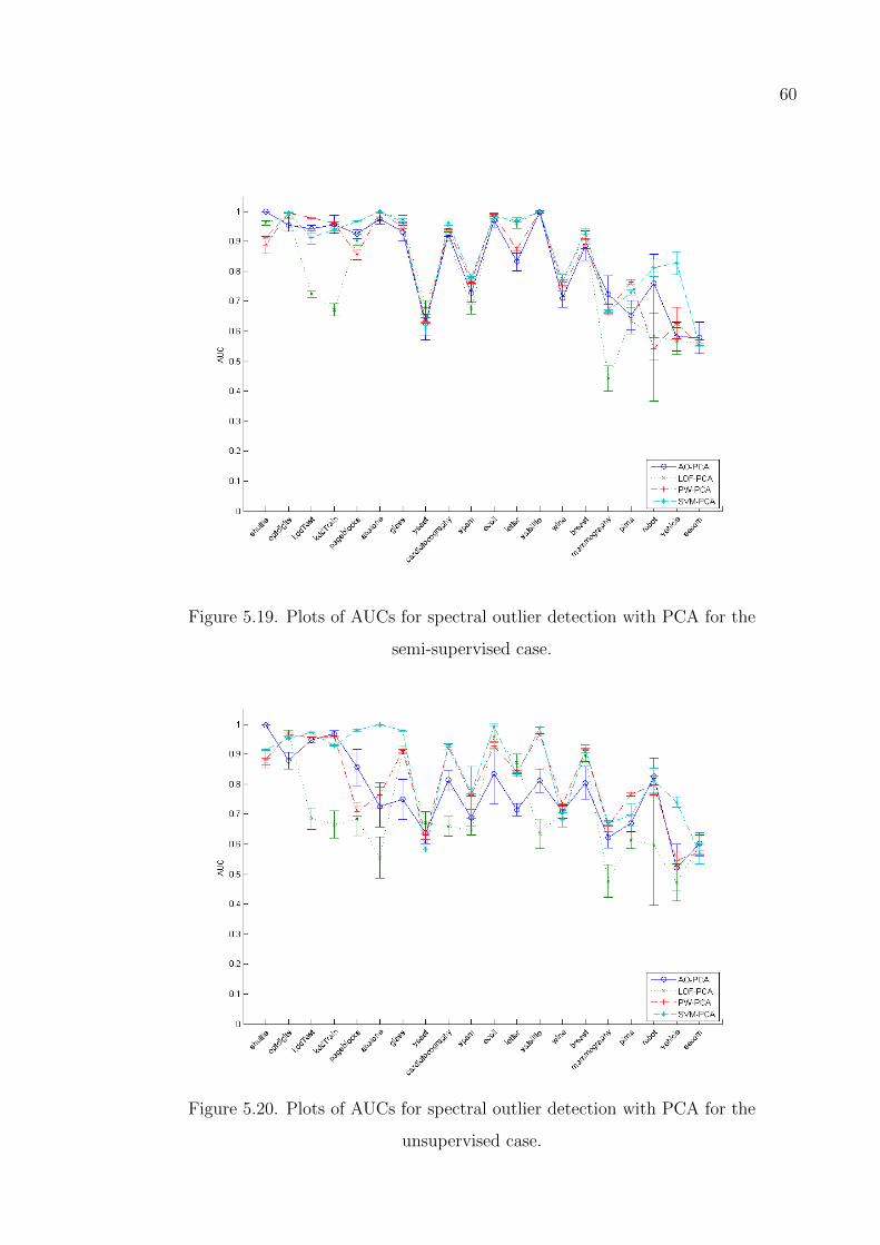
60

Figure 5.19. Plots of AUCs for spectral outlier detection with PCA for the

semi-supervised case.

Figure 5.20. Plots of AUCs for spectral outlier detection with PCA for the

unsupervised case.

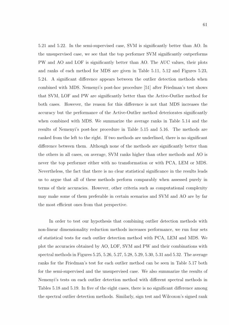
61

5.21 and 5.22. In the semi-supervised case, SVM is significantly better than AO. In

the unsupervised case, we see that the top performer SVM significantly outperforms

PW and AO and LOF is significantly better than AO. The AUC values, their plots

and ranks of each method for MDS are given in Table 5.11, 5.12 and Figures 5.23,

5.24. A significant difference appears between the outlier detection methods when

combined with MDS. Nemenyi’s post-hoc procedure [51] after Friedman’s test shows

that SVM, LOF and PW are significantly better than the Active-Outlier method for

both cases. However, the reason for this difference is not that MDS increases the

accuracy but the performance of the Active-Outlier method deteriorates significantly

when combined with MDS. We summarize the average ranks in Table 5.14 and the

results of Nemenyi’s post-hoc procedure in Table 5.15 and 5.16. The methods are

ranked from the left to the right. If two methods are underlined, there is no significant

difference between them. Although none of the methods are significantly better than

the others in all cases, on average, SVM ranks higher than other methods and AO is

never the top performer either with no transformation or with PCA, LEM or MDS.

Nevertheless, the fact that there is no clear statistical significance in the results leads

us to argue that all of these methods perform comparably when assessed purely in

terms of their accuracies. However, other criteria such as computational complexity

may make some of them preferable in certain scenarios and SVM and AO are by far

the most efficient ones from that perspective.

In order to test our hypothesis that combining outlier detection methods with

non-linear dimensionality reduction methods increases performance, we run four sets

of statistical tests for each outlier detection method with PCA, LEM and MDS. We

plot the accuracies obtained by AO, LOF, SVM and PW and their combinations with

spectral methods in Figures 5.25, 5.26, 5.27, 5.28, 5.29, 5.30, 5.31 and 5.32. The average

ranks for the Friedman’s test for each outlier method can be seen in Table 5.17 both

for the semi-supervised and the unsupervised case. We also summarize the results of

Nemenyi’s tests on each outlier detection method with different spectral methods in

Tables 5.18 and 5.19. In five of the eight cases, there is no significant difference among

the spectral outlier detection methods. Similarly, sign test and Wilcoxon’s signed rank

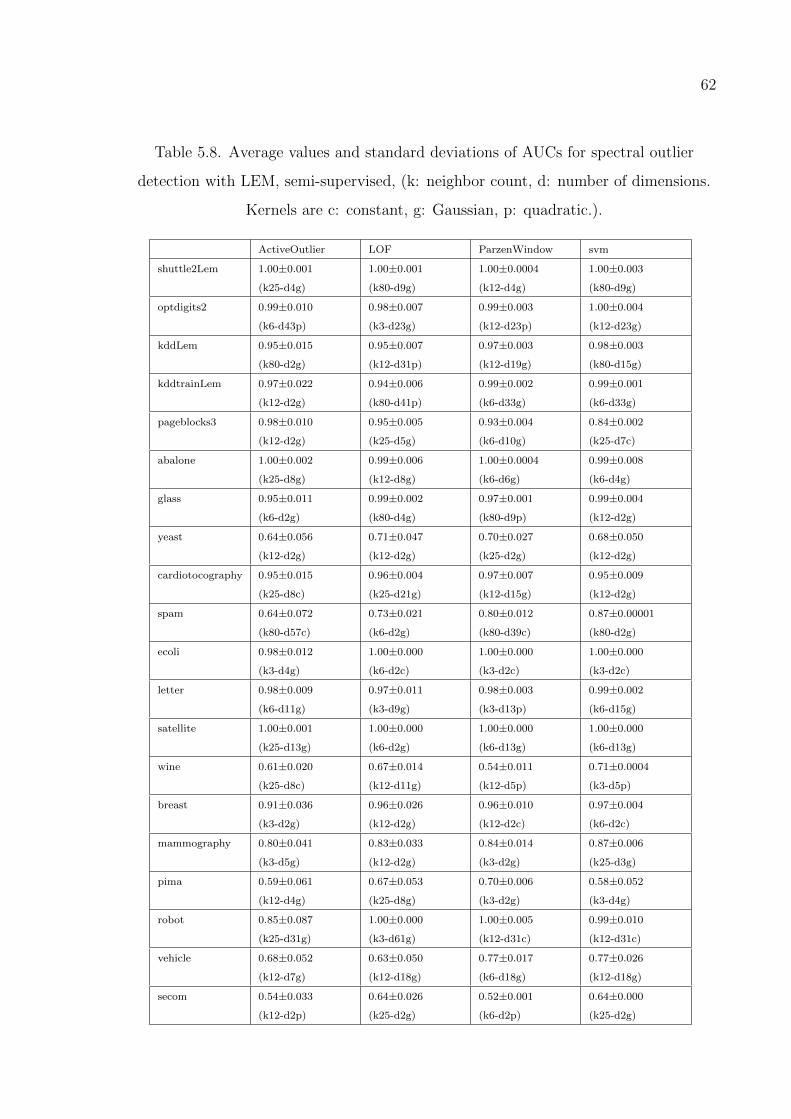
62

Table 5.8. Average values and standard deviations of AUCs for spectral outlier

detection with LEM, semi-supervised, (k: neighbor count, d: number of dimensions.

Kernels are c: constant, g: Gaussian, p: quadratic.).

ActiveOutlier LOF ParzenWindow svm

shuttle2Lem 1.00±0.001

(k25-d4g)

1.00±0.001

(k80-d9g)

1.00±0.0004

(k12-d4g)

1.00±0.003

(k80-d9g)

optdigits2 0.99±0.010

(k6-d43p)

0.98±0.007

(k3-d23g)

0.99±0.003

(k12-d23p)

1.00±0.004

(k12-d23g)

kddLem 0.95±0.015

(k80-d2g)

0.95±0.007

(k12-d31p)

0.97±0.003

(k12-d19g)

0.98±0.003

(k80-d15g)

kddtrainLem 0.97±0.022

(k12-d2g)

0.94±0.006

(k80-d41p)

0.99±0.002

(k6-d33g)

0.99±0.001

(k6-d33g)

pageblocks3 0.98±0.010

(k12-d2g)

0.95±0.005

(k25-d5g)

0.93±0.004

(k6-d10g)

0.84±0.002

(k25-d7c)

abalone 1.00±0.002

(k25-d8g)

0.99±0.006

(k12-d8g)

1.00±0.0004

(k6-d6g)

0.99±0.008

(k6-d4g)

glass 0.95±0.011

(k6-d2g)

0.99±0.002

(k80-d4g)

0.97±0.001

(k80-d9p)

0.99±0.004

(k12-d2g)

yeast 0.64±0.056

(k12-d2g)

0.71±0.047

(k12-d2g)

0.70±0.027

(k25-d2g)

0.68±0.050

(k12-d2g)

cardiotocography 0.95±0.015

(k25-d8c)

0.96±0.004

(k25-d21g)

0.97±0.007

(k12-d15g)

0.95±0.009

(k12-d2g)

spam 0.64±0.072

(k80-d57c)

0.73±0.021

(k6-d2g)

0.80±0.012

(k80-d39c)

0.87±0.00001

(k80-d2g)

ecoli 0.98±0.012

(k3-d4g)

1.00±0.000

(k6-d2c)

1.00±0.000

(k3-d2c)

1.00±0.000

(k3-d2c)

letter 0.98±0.009

(k6-d11g)

0.97±0.011

(k3-d9g)

0.98±0.003

(k3-d13p)

0.99±0.002

(k6-d15g)

satellite 1.00±0.001

(k25-d13g)

1.00±0.000

(k6-d2g)

1.00±0.000

(k6-d13g)

1.00±0.000

(k6-d13g)

wine 0.61±0.020

(k25-d8c)

0.67±0.014

(k12-d11g)

0.54±0.011

(k12-d5p)

0.71±0.0004

(k3-d5p)

breast 0.91±0.036

(k3-d2g)

0.96±0.026

(k12-d2g)

0.96±0.010

(k12-d2c)

0.97±0.004

(k6-d2c)

mammography 0.80±0.041

(k3-d5g)

0.83±0.033

(k12-d2g)

0.84±0.014

(k3-d2g)

0.87±0.006

(k25-d3g)

pima 0.59±0.061

(k12-d4g)

0.67±0.053

(k25-d8g)

0.70±0.006

(k3-d2g)

0.58±0.052

(k3-d4g)

robot 0.85±0.087

(k25-d31g)

1.00±0.000

(k3-d61g)

1.00±0.005

(k12-d31c)

0.99±0.010

(k12-d31c)

vehicle 0.68±0.052

(k12-d7g)

0.63±0.050

(k12-d18g)

0.77±0.017

(k6-d18g)

0.77±0.026

(k12-d18g)

secom 0.54±0.033

(k12-d2p)

0.64±0.026

(k25-d2g)

0.52±0.001

(k6-d2p)

0.64±0.000

(k25-d2g)

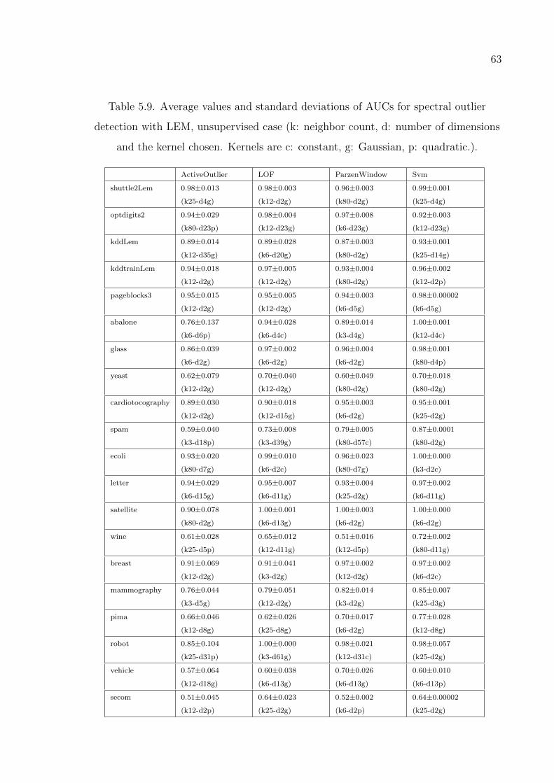
63

Table 5.9. Average values and standard deviations of AUCs for spectral outlier

detection with LEM, unsupervised case (k: neighbor count, d: number of dimensions

and the kernel chosen. Kernels are c: constant, g: Gaussian, p: quadratic.).

ActiveOutlier LOF ParzenWindow Svm

shuttle2Lem 0.98±0.013

(k25-d4g)

0.98±0.003

(k12-d2g)

0.96±0.003

(k80-d2g)

0.99±0.001

(k25-d4g)

optdigits2 0.94±0.029

(k80-d23p)

0.98±0.004

(k12-d23g)

0.97±0.008

(k6-d23g)

0.92±0.003

(k12-d23g)

kddLem 0.89±0.014

(k12-d35g)

0.89±0.028

(k6-d20g)

0.87±0.003

(k80-d2g)

0.93±0.001

(k25-d14g)

kddtrainLem 0.94±0.018

(k12-d2g)

0.97±0.005

(k12-d2g)

0.93±0.004

(k80-d2g)

0.96±0.002

(k12-d2p)

pageblocks3 0.95±0.015

(k12-d2g)

0.95±0.005

(k12-d2g)

0.94±0.003

(k6-d5g)

0.98±0.00002

(k6-d5g)

abalone 0.76±0.137

(k6-d6p)

0.94±0.028

(k6-d4c)

0.89±0.014

(k3-d4g)

1.00±0.001

(k12-d4c)

glass 0.86±0.039

(k6-d2g)

0.97±0.002

(k6-d2g)

0.96±0.004

(k6-d2g)

0.98±0.001

(k80-d4p)

yeast 0.62±0.079

(k12-d2g)

0.70±0.040

(k12-d2g)

0.60±0.049

(k80-d2g)

0.70±0.018

(k80-d2g)

cardiotocography 0.89±0.030

(k12-d2g)

0.90±0.018

(k12-d15g)

0.95±0.003

(k6-d2g)

0.95±0.001

(k25-d2g)

spam 0.59±0.040

(k3-d18p)

0.73±0.008

(k3-d39g)

0.79±0.005

(k80-d57c)

0.87±0.0001

(k80-d2g)

ecoli 0.93±0.020

(k80-d7g)

0.99±0.010

(k6-d2c)

0.96±0.023

(k80-d7g)

1.00±0.000

(k3-d2c)

letter 0.94±0.029

(k6-d15g)

0.95±0.007

(k6-d11g)

0.93±0.004

(k25-d2g)

0.97±0.002

(k6-d11g)

satellite 0.90±0.078

(k80-d2g)

1.00±0.001

(k6-d13g)

1.00±0.003

(k6-d2g)

1.00±0.000

(k6-d2g)

wine 0.61±0.028

(k25-d5p)

0.65±0.012

(k12-d11g)

0.51±0.016

(k12-d5p)

0.72±0.002

(k80-d11g)

breast 0.91±0.069

(k12-d2g)

0.91±0.041

(k3-d2g)

0.97±0.002

(k12-d2g)

0.97±0.002

(k6-d2c)

mammography 0.76±0.044

(k3-d5g)

0.79±0.051

(k12-d2g)

0.82±0.014

(k3-d2g)

0.85±0.007

(k25-d3g)

pima 0.66±0.046

(k12-d8g)

0.62±0.026

(k25-d8g)

0.70±0.017

(k6-d2g)

0.77±0.028

(k12-d8g)

robot 0.85±0.104

(k25-d31p)

1.00±0.000

(k3-d61g)

0.98±0.021

(k12-d31c)

0.98±0.057

(k25-d2g)

vehicle 0.57±0.064

(k12-d18g)

0.60±0.038

(k6-d13g)

0.70±0.026

(k6-d13g)

0.60±0.010

(k6-d13p)

secom 0.51±0.045

(k12-d2p)

0.64±0.023

(k25-d2g)

0.52±0.002

(k6-d2p)

0.64±0.00002

(k25-d2g)

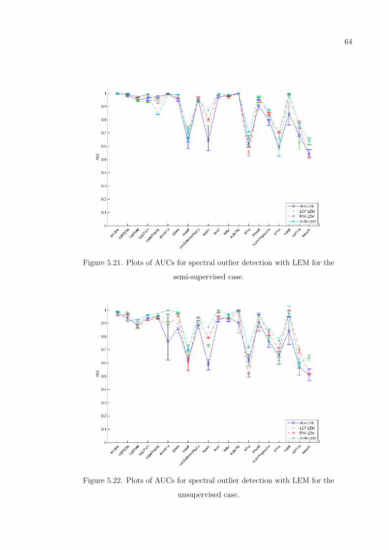
64

Figure 5.21. Plots of AUCs for spectral outlier detection with LEM for the

semi-supervised case.

Figure 5.22. Plots of AUCs for spectral outlier detection with LEM for the

unsupervised case.

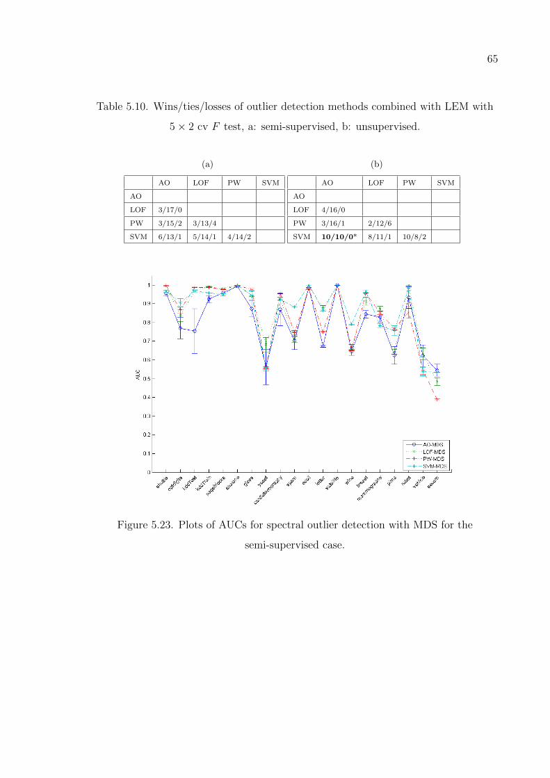
65

Table 5.10. Wins/ties/losses of outlier detection methods combined with LEM with

5× 2 cv F test, a: semi-supervised, b: unsupervised.

(a)

AO LOF PW SVM

AO

LOF 3/17/0

PW 3/15/2 3/13/4

SVM 6/13/1 5/14/1 4/14/2

(b)

AO LOF PW SVM

AO

LOF 4/16/0

PW 3/16/1 2/12/6

SVM 10/10/0* 8/11/1 10/8/2

Figure 5.23. Plots of AUCs for spectral outlier detection with MDS for the

semi-supervised case.

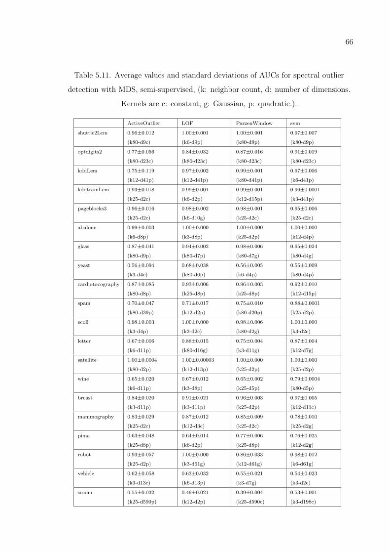
66

Table 5.11. Average values and standard deviations of AUCs for spectral outlier

detection with MDS, semi-supervised, (k: neighbor count, d: number of dimensions.

Kernels are c: constant, g: Gaussian, p: quadratic.).

ActiveOutlier LOF ParzenWindow svm

shuttle2Lem 0.96±0.012

(k80-d9c)

1.00±0.001

(k6-d9p)

1.00±0.001

(k80-d9p)

0.97±0.007

(k80-d9p)

optdigits2 0.77±0.056

(k80-d23c)

0.84±0.032

(k80-d23c)

0.87±0.016

(k80-d23c)

0.91±0.019

(k80-d23c)

kddLem 0.75±0.119

(k12-d41p)

0.97±0.002

(k12-d41p)

0.99±0.001

(k80-d41p)

0.97±0.006

(k6-d41p)

kddtrainLem 0.93±0.018

(k25-d2c)

0.99±0.001

(k6-d2p)

0.99±0.001

(k12-d15p)

0.96±0.0001

(k3-d41p)

pageblocks3 0.96±0.016

(k25-d2c)

0.98±0.002

(k6-d10g)

0.98±0.001

(k25-d2c)

0.95±0.006

(k25-d2c)

abalone 0.99±0.003

(k6-d8p)

1.00±0.000

(k3-d8p)

1.00±0.000

(k25-d2p)

1.00±0.000

(k12-d4p)

glass 0.87±0.041

(k80-d9p)

0.94±0.002

(k80-d7p)

0.98±0.006

(k80-d7g)

0.95±0.024

(k80-d4g)

yeast 0.56±0.094

(k3-d4c)

0.68±0.038

(k80-d6p)

0.56±0.005

(k6-d4p)

0.55±0.009

(k80-d4p)

cardiotocography 0.87±0.085

(k80-d8p)

0.93±0.006

(k25-d8p)

0.96±0.003

(k25-d8p)

0.92±0.010

(k12-d15p)

spam 0.70±0.047

(k80-d39p)

0.71±0.017

(k12-d2p)

0.75±0.010

(k80-d20p)

0.88±0.0001

(k25-d2p)

ecoli 0.98±0.003

(k3-d4p)

1.00±0.000

(k3-d2c)

0.98±0.006

(k80-d2g)

1.00±0.000

(k3-d2c)

letter 0.67±0.006

(k6-d11p)

0.88±0.015

(k80-d16g)

0.75±0.004

(k3-d11g)

0.87±0.004

(k12-d7g)

satellite 1.00±0.0004

(k80-d2p)

1.00±0.00003

(k12-d13p)

1.00±0.000

(k25-d2p)

1.00±0.000

(k25-d2p)

wine 0.65±0.020

(k6-d11p)

0.67±0.012

(k3-d8p)

0.65±0.002

(k25-d5p)

0.79±0.0004

(k80-d5p)

breast 0.84±0.020

(k3-d11p)

0.91±0.021

(k3-d11p)

0.96±0.003

(k25-d2p)

0.97±0.005

(k12-d11c)

mammography 0.83±0.029

(k25-d2c)

0.87±0.012

(k12-d3c)

0.85±0.009

(k25-d2c)

0.78±0.010

(k25-d2g)

pima 0.63±0.048

(k25-d8p)

0.64±0.014

(k6-d2p)

0.77±0.006

(k25-d8p)

0.76±0.025

(k12-d2g)

robot 0.93±0.057

(k25-d2p)

1.00±0.000

(k3-d61g)

0.86±0.033

(k12-d61g)

0.98±0.012

(k6-d61g)

vehicle 0.62±0.058

(k3-d13c)

0.63±0.032

(k6-d13p)

0.55±0.021

(k3-d7g)

0.54±0.023

(k3-d2c)

secom 0.55±0.032

(k25-d590p)

0.49±0.021

(k12-d2p)

0.39±0.004

(k25-d590c)

0.53±0.001

(k3-d198c)

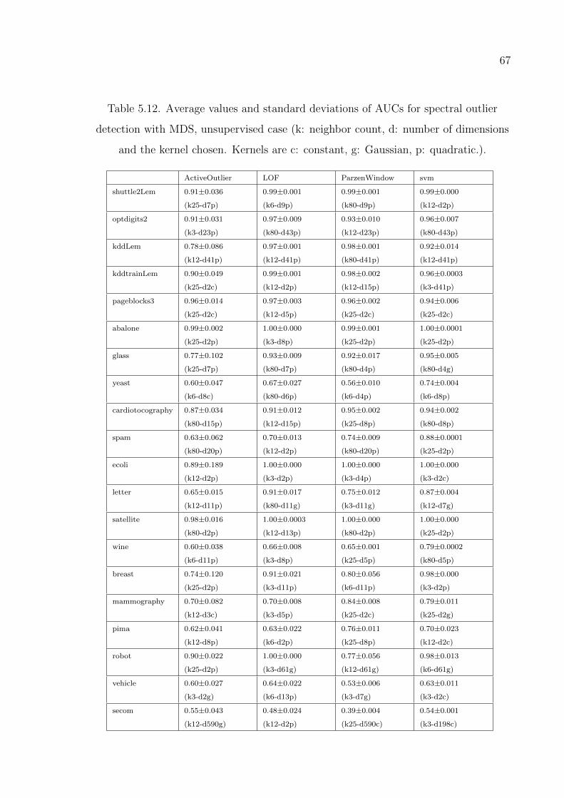
67

Table 5.12. Average values and standard deviations of AUCs for spectral outlier

detection with MDS, unsupervised case (k: neighbor count, d: number of dimensions

and the kernel chosen. Kernels are c: constant, g: Gaussian, p: quadratic.).

ActiveOutlier LOF ParzenWindow svm

shuttle2Lem 0.91±0.036

(k25-d7p)

0.99±0.001

(k6-d9p)

0.99±0.001

(k80-d9p)

0.99±0.000

(k12-d2p)

optdigits2 0.91±0.031

(k3-d23p)

0.97±0.009

(k80-d43p)

0.93±0.010

(k12-d23p)

0.96±0.007

(k80-d43p)

kddLem 0.78±0.086

(k12-d41p)

0.97±0.001

(k12-d41p)

0.98±0.001

(k80-d41p)

0.92±0.014

(k12-d41p)

kddtrainLem 0.90±0.049

(k25-d2c)

0.99±0.001

(k12-d2p)

0.98±0.002

(k12-d15p)

0.96±0.0003

(k3-d41p)

pageblocks3 0.96±0.014

(k25-d2c)

0.97±0.003

(k12-d5p)

0.96±0.002

(k25-d2c)

0.94±0.006

(k25-d2c)

abalone 0.99±0.002

(k25-d2p)

1.00±0.000

(k3-d8p)

0.99±0.001

(k25-d2p)

1.00±0.0001

(k25-d2p)

glass 0.77±0.102

(k25-d7p)

0.93±0.009

(k80-d7p)

0.92±0.017

(k80-d4p)

0.95±0.005

(k80-d4g)

yeast 0.60±0.047

(k6-d8c)

0.67±0.027

(k80-d6p)

0.56±0.010

(k6-d4p)

0.74±0.004

(k6-d8p)

cardiotocography 0.87±0.034

(k80-d15p)

0.91±0.012

(k12-d15p)

0.95±0.002

(k25-d8p)

0.94±0.002

(k80-d8p)

spam 0.63±0.062

(k80-d20p)

0.70±0.013

(k12-d2p)

0.74±0.009

(k80-d20p)

0.88±0.0001

(k25-d2p)

ecoli 0.89±0.189

(k12-d2p)

1.00±0.000

(k3-d2p)

1.00±0.000

(k3-d4p)

1.00±0.000

(k3-d2c)

letter 0.65±0.015

(k12-d11p)

0.91±0.017

(k80-d11g)

0.75±0.012

(k3-d11g)

0.87±0.004

(k12-d7g)

satellite 0.98±0.016

(k80-d2p)

1.00±0.0003

(k12-d13p)

1.00±0.000

(k80-d2p)

1.00±0.000

(k25-d2p)

wine 0.60±0.038

(k6-d11p)

0.66±0.008

(k3-d8p)

0.65±0.001

(k25-d5p)

0.79±0.0002

(k80-d5p)

breast 0.74±0.120

(k25-d2p)

0.91±0.021

(k3-d11p)

0.80±0.056

(k6-d11p)

0.98±0.000

(k3-d2p)

mammography 0.70±0.082

(k12-d3c)

0.70±0.008

(k3-d5p)

0.84±0.008

(k25-d2c)

0.79±0.011

(k25-d2g)

pima 0.62±0.041

(k12-d8p)

0.63±0.022

(k6-d2p)

0.76±0.011

(k25-d8p)

0.70±0.023

(k12-d2c)

robot 0.90±0.022

(k25-d2p)

1.00±0.000

(k3-d61g)

0.77±0.056

(k12-d61g)

0.98±0.013

(k6-d61g)

vehicle 0.60±0.027

(k3-d2g)

0.64±0.022

(k6-d13p)

0.53±0.006

(k3-d7g)

0.63±0.011

(k3-d2c)

secom 0.55±0.043

(k12-d590g)

0.48±0.024

(k12-d2p)

0.39±0.004

(k25-d590c)

0.54±0.001

(k3-d198c)

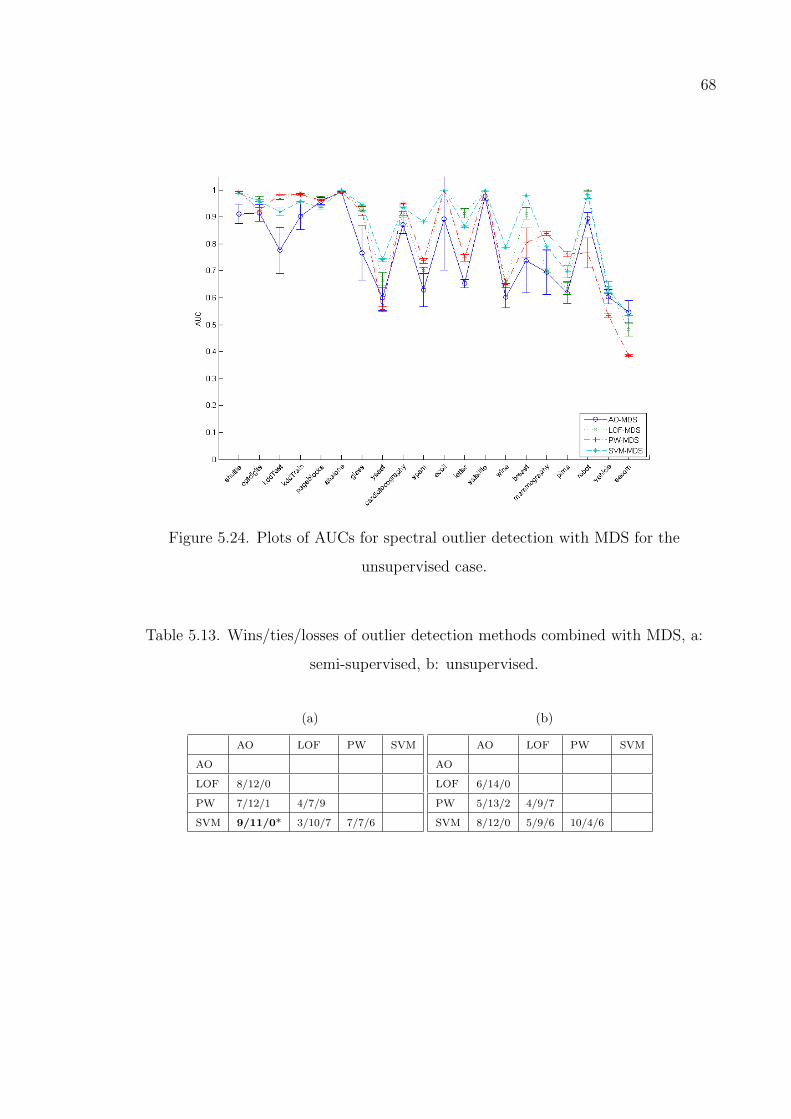
68

Figure 5.24. Plots of AUCs for spectral outlier detection with MDS for the

unsupervised case.

Table 5.13. Wins/ties/losses of outlier detection methods combined with MDS, a:

semi-supervised, b: unsupervised.

(a)

AO LOF PW SVM

AO

LOF 8/12/0

PW 7/12/1 4/7/9

SVM 9/11/0* 3/10/7 7/7/6

(b)

AO LOF PW SVM

AO

LOF 6/14/0

PW 5/13/2 4/9/7

SVM 8/12/0 5/9/6 10/4/6

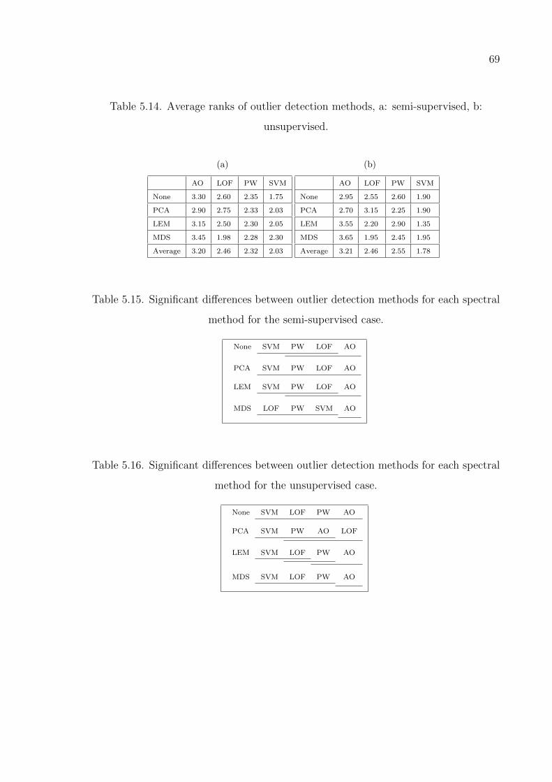
69

Table 5.14. Average ranks of outlier detection methods, a: semi-supervised, b:

unsupervised.

(a)

AO LOF PW SVM

None 3.30 2.60 2.35 1.75

PCA 2.90 2.75 2.33 2.03

LEM 3.15 2.50 2.30 2.05

MDS 3.45 1.98 2.28 2.30

Average 3.20 2.46 2.32 2.03

(b)

AO LOF PW SVM

None 2.95 2.55 2.60 1.90

PCA 2.70 3.15 2.25 1.90

LEM 3.55 2.20 2.90 1.35

MDS 3.65 1.95 2.45 1.95

Average 3.21 2.46 2.55 1.78

Table 5.15. Significant differences between outlier detection methods for each spectral

method for the semi-supervised case.

None SVM PW LOF AO

PCA SVM PW LOF AO

LEM SVM PW LOF AO

MDS LOF PW SVM AO

Table 5.16. Significant differences between outlier detection methods for each spectral

method for the unsupervised case.

None SVM LOF PW AO

PCA SVM PW AO LOF

LEM SVM LOF PW AO

MDS SVM LOF PW AO

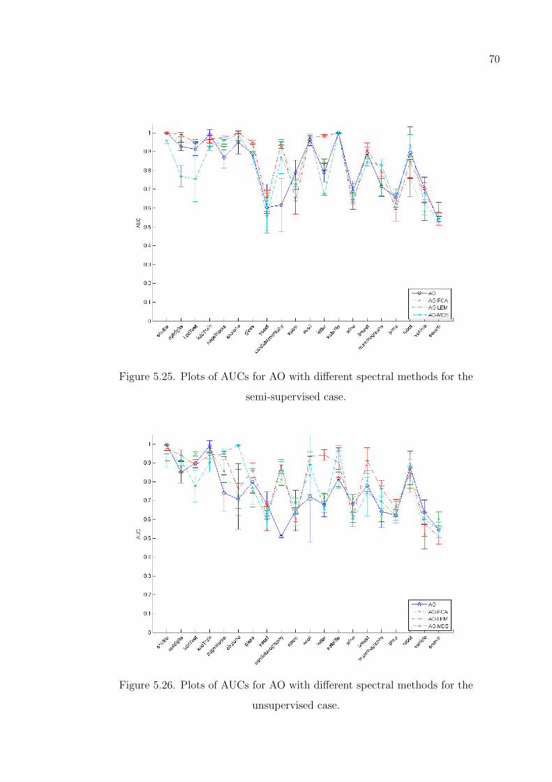
70

Figure 5.25. Plots of AUCs for AO with different spectral methods for the

semi-supervised case.

Figure 5.26. Plots of AUCs for AO with different spectral methods for the

unsupervised case.

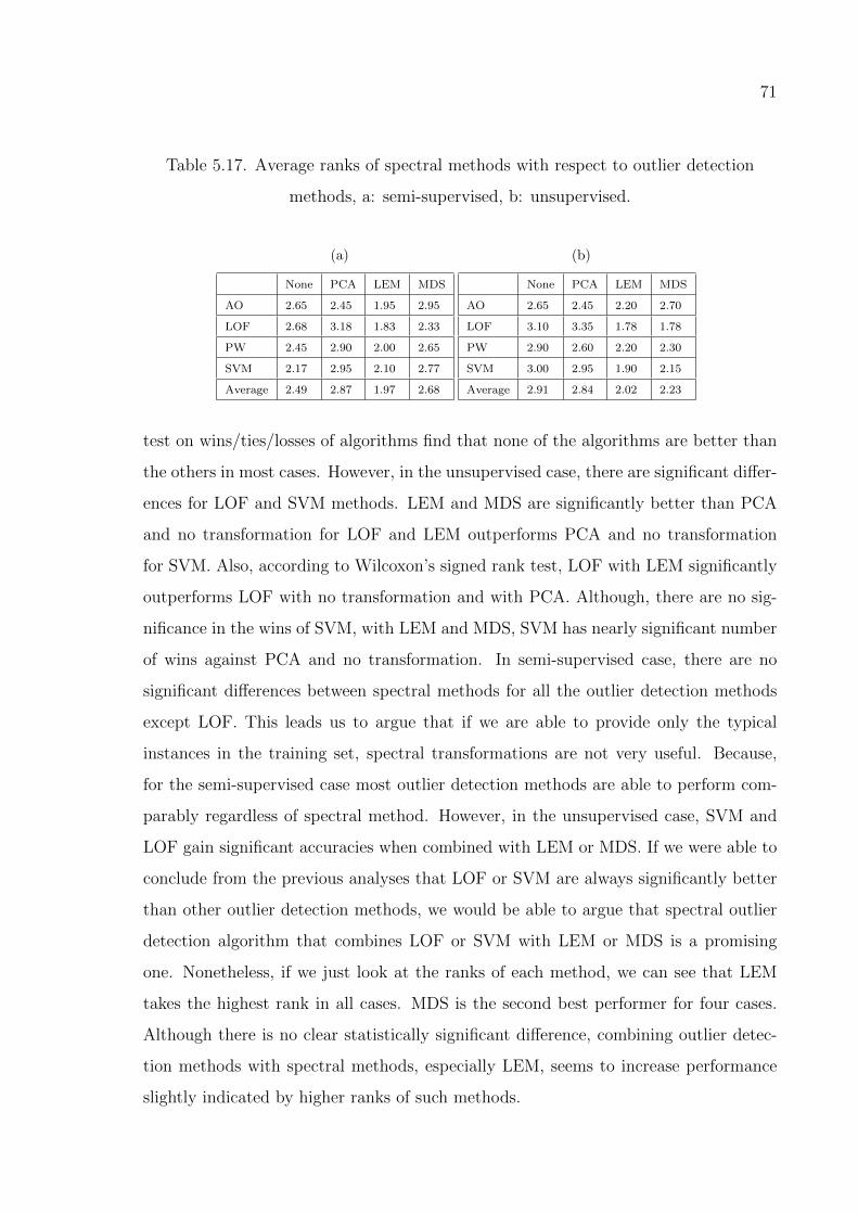
71

Table 5.17. Average ranks of spectral methods with respect to outlier detection

methods, a: semi-supervised, b: unsupervised.

(a)

None PCA LEM MDS

AO 2.65 2.45 1.95 2.95

LOF 2.68 3.18 1.83 2.33

PW 2.45 2.90 2.00 2.65

SVM 2.17 2.95 2.10 2.77

Average 2.49 2.87 1.97 2.68

(b)

None PCA LEM MDS

AO 2.65 2.45 2.20 2.70

LOF 3.10 3.35 1.78 1.78

PW 2.90 2.60 2.20 2.30

SVM 3.00 2.95 1.90 2.15

Average 2.91 2.84 2.02 2.23

test on wins/ties/losses of algorithms find that none of the algorithms are better than

the others in most cases. However, in the unsupervised case, there are significant differ-

ences for LOF and SVM methods. LEM and MDS are significantly better than PCA

and no transformation for LOF and LEM outperforms PCA and no transformation

for SVM. Also, according to Wilcoxon’s signed rank test, LOF with LEM significantly

outperforms LOF with no transformation and with PCA. Although, there are no sig-

nificance in the wins of SVM, with LEM and MDS, SVM has nearly significant number

of wins against PCA and no transformation. In semi-supervised case, there are no

significant differences between spectral methods for all the outlier detection methods

except LOF. This leads us to argue that if we are able to provide only the typical

instances in the training set, spectral transformations are not very useful. Because,

for the semi-supervised case most outlier detection methods are able to perform com-

parably regardless of spectral method. However, in the unsupervised case, SVM and

LOF gain significant accuracies when combined with LEM or MDS. If we were able to

conclude from the previous analyses that LOF or SVM are always significantly better

than other outlier detection methods, we would be able to argue that spectral outlier

detection algorithm that combines LOF or SVM with LEM or MDS is a promising

one. Nonetheless, if we just look at the ranks of each method, we can see that LEM

takes the highest rank in all cases. MDS is the second best performer for four cases.

Although there is no clear statistically significant difference, combining outlier detec-

tion methods with spectral methods, especially LEM, seems to increase performance

slightly indicated by higher ranks of such methods.

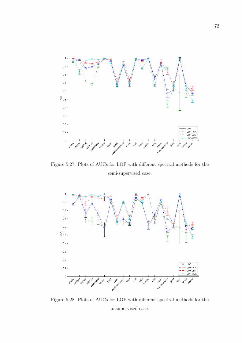
72

Figure 5.27. Plots of AUCs for LOF with different spectral methods for the

semi-supervised case.

Figure 5.28. Plots of AUCs for LOF with different spectral methods for the

unsupervised case.

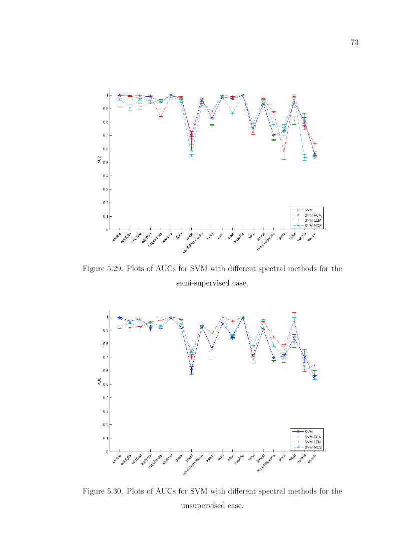
73

Figure 5.29. Plots of AUCs for SVM with different spectral methods for the

semi-supervised case.

Figure 5.30. Plots of AUCs for SVM with different spectral methods for the

unsupervised case.

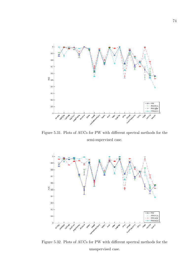
74

Figure 5.31. Plots of AUCs for PW with different spectral methods for the

semi-supervised case.

Figure 5.32. Plots of AUCs for PW with different spectral methods for the

unsupervised case.

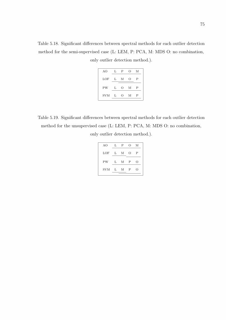
75

Table 5.18. Significant differences between spectral methods for each outlier detection

method for the semi-supervised case (L: LEM, P: PCA, M: MDS O: no combination,

only outlier detection method.).

AO L P O M

LOF L M O P

PW L O M P

SVM L O M P

Table 5.19. Significant differences between spectral methods for each outlier detection

method for the unsupervised case (L: LEM, P: PCA, M: MDS O: no combination,

only outlier detection method.).

AO L P O M

LOF L M O P

PW L M P O

SVM L M P O

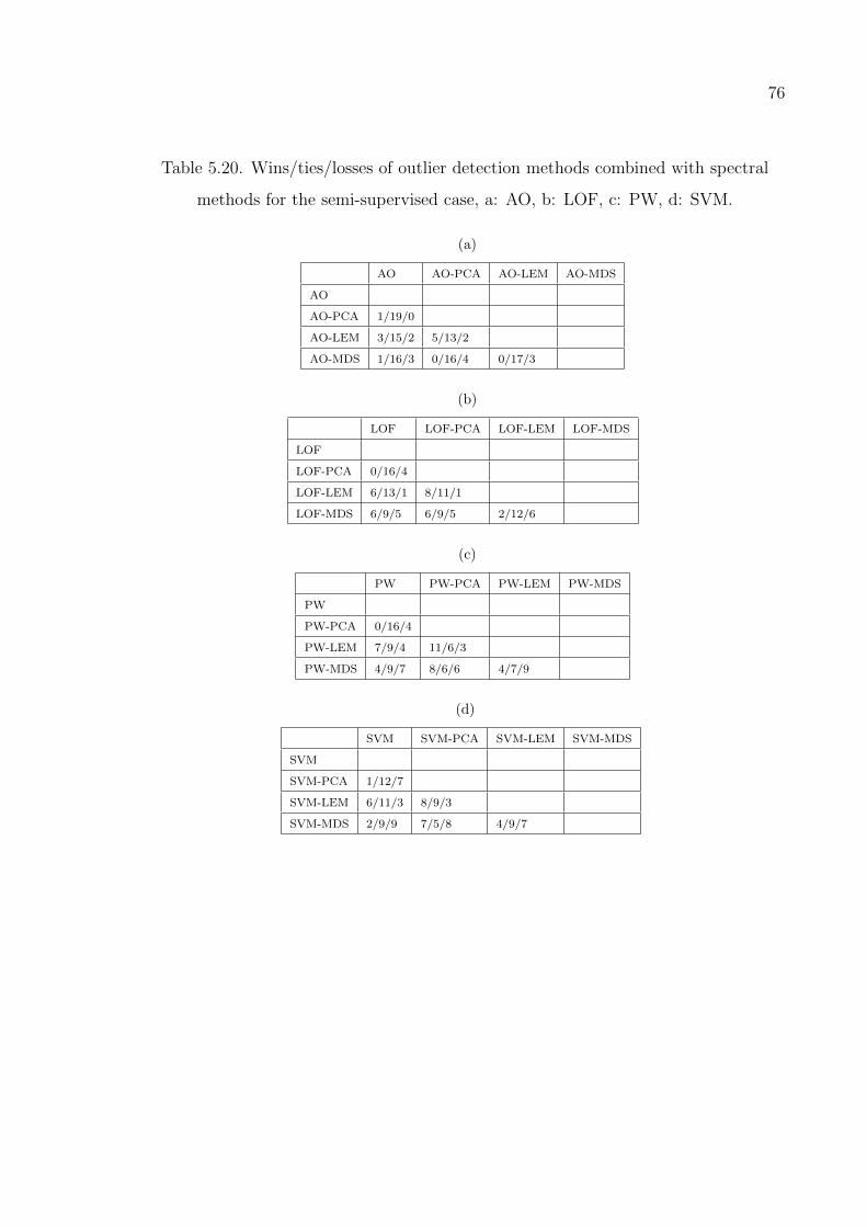
76

Table 5.20. Wins/ties/losses of outlier detection methods combined with spectral

methods for the semi-supervised case, a: AO, b: LOF, c: PW, d: SVM.

(a)

AO AO-PCA AO-LEM AO-MDS

AO

AO-PCA 1/19/0

AO-LEM 3/15/2 5/13/2

AO-MDS 1/16/3 0/16/4 0/17/3

(b)

LOF LOF-PCA LOF-LEM LOF-MDS

LOF

LOF-PCA 0/16/4

LOF-LEM 6/13/1 8/11/1

LOF-MDS 6/9/5 6/9/5 2/12/6

(c)

PW PW-PCA PW-LEM PW-MDS

PW

PW-PCA 0/16/4

PW-LEM 7/9/4 11/6/3

PW-MDS 4/9/7 8/6/6 4/7/9

(d)

SVM SVM-PCA SVM-LEM SVM-MDS

SVM

SVM-PCA 1/12/7

SVM-LEM 6/11/3 8/9/3

SVM-MDS 2/9/9 7/5/8 4/9/7

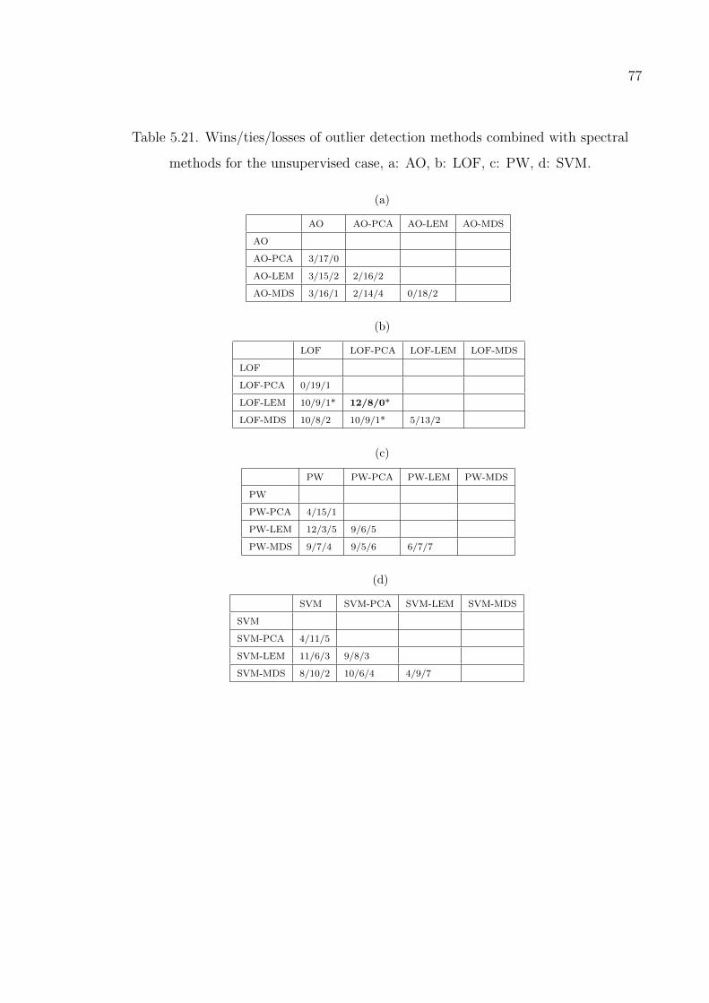
77

Table 5.21. Wins/ties/losses of outlier detection methods combined with spectral

methods for the unsupervised case, a: AO, b: LOF, c: PW, d: SVM.

(a)

AO AO-PCA AO-LEM AO-MDS

AO

AO-PCA 3/17/0

AO-LEM 3/15/2 2/16/2

AO-MDS 3/16/1 2/14/4 0/18/2

(b)

LOF LOF-PCA LOF-LEM LOF-MDS

LOF

LOF-PCA 0/19/1

LOF-LEM 10/9/1* 12/8/0*

LOF-MDS 10/8/2 10/9/1* 5/13/2

(c)

PW PW-PCA PW-LEM PW-MDS

PW

PW-PCA 4/15/1

PW-LEM 12/3/5 9/6/5

PW-MDS 9/7/4 9/5/6 6/7/7

(d)

SVM SVM-PCA SVM-LEM SVM-MDS

SVM

SVM-PCA 4/11/5

SVM-LEM 11/6/3 9/8/3

SVM-MDS 8/10/2 10/6/4 4/9/7

78

5.4. Face Detection

We evaluate our spectral outlier detection method on a face detection problem.

CBCL Face Detection data set [52] contains 19× 19 images of face and non-faces. The

training set contains 291 instances from the face class and the test set consists of 124

face and 1205 non-face instances. The typical class is considered to be the face class.

We evaluate the accuracy of the Active-Outlier method individually and with PCA

and LEM. With no transformation, AUC is 0.85 while PCA reports 0.76. The spectral

outlier detection approach with LEM significantly increases accuracy and reaches 0.97.

Furthermore, LEM reaches this reported accuracy using only two dimensions. We also

plot the instances in two dimensions, seen in Figures 5.34 and 5.33, to show that the

transformation achieved by LEM is superior to PCA.

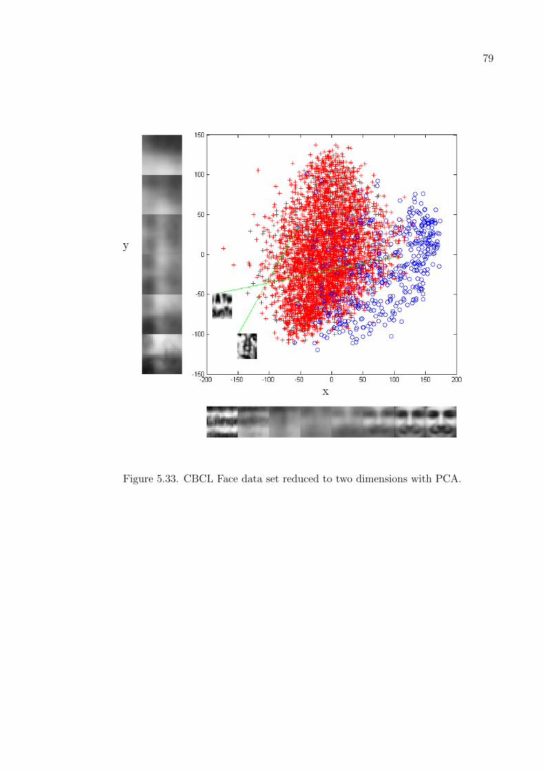
79

Figure 5.33. CBCL Face data set reduced to two dimensions with PCA.

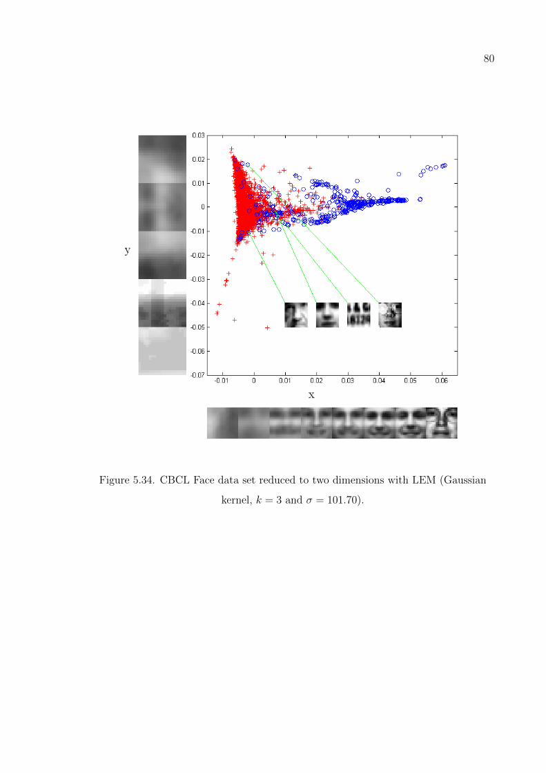
80

Figure 5.34. CBCL Face data set reduced to two dimensions with LEM (Gaussian

kernel, k = 3 and σ = 101.70).

81

6. CONCLUSIONS AND FUTURE WORK

In this thesis, we propose a new method for outlier detection. Reducing the di-

mensionality of the data and transforming it to get a representation where the outliers

are more easily identifiable has been shown to increase accuracy in previous works.

We argue that the ability of spectral methods to reveal the non-linear structure in the

data would be valuable for outlier detection. We review various spectral methods and

discuss the similarities and the differences between them. Our spectral outlier detec-

tion algorithm involves having a spectral method before outlier detection. In order to

evaluate the performance of our method, we carry out experiments on 20 data sets with

four different outlier detection methods. The results of our experiments show us that

although SVM seems to perform well overall, none of the outlier detection methods is

significantly superior to the others and choosing the best one depends heavily on the

specific setting of the problem in question.

All the methods discussed in this thesis, for outlier detection and spectral de-

composition are implemented in MATLAB and this toolbox is made available; details

are given in Appendix A.

When we compare the different combinations of outlier detection methods with

spectral methods, we see that the performance differences between methods vanish

in the semi-supervised case. This leads us to argue that all the methods are able to

perform comparably well when only the typical data are given in the training set. The

differences between methods appear in the unsupervised case, which is a more realistic

scenario for outlier detection, since, most of the time we do not have labelled data.

In the unsupervised case, using spectral transformation beforehand does not affect the

accuracies of AO or PW much. This is expected for AO, because, it never deals with

the distribution of input data and thus is not affected by it. The reason for similar

performances in the case of PW with different spectral methods can be attributed to

the fact that all of the spectral methods preserve local information in the data. So, it

82

is possible to find a parameter for PW method that gives good results in different input

spaces. However, spectral transformations have an effect on the performances of LOF

and SVM. The increase in LOF’s performance when combined with LEM probably

stems from the fact that LEM maps similar instances to closer points in the new space.

This property increases the differences in the local densities, hence, making it easier

to find outliers. Since the transformed instances are contained in a smaller volume

compared to the original input space, SVM is also able to learn a smoother function.

Therefore, by combining SVM or LOF with LEM, we are able to increase the outlier

detection accuracy. If we compare SVM with LOF, we can say that SVM usually

outperforms LOF and more importantly, being a discriminative method, SVM has a

significantly lower time complexity.

Due to the ambiguity of the outlier concept and the lack of available data sets, we

assumed the rare class classification approach for creating outlier detection problems.

We have a very diverse set of data sets where some are artificial problems and most of

them are actually not really outlier detection problems. There are even some data sets

that have such high outlier percentages that it may not be rational to consider them

outlier detection problems. More importantly, since we assume that the instances from

the rare class to be outliers, outliers form clusters which is not quite realistic.

As future work, a more solid analysis from the perspective of spectral meth-

ods is possible that looks at the performances according to the properties of the data

sets. Analyzing the data sets that LOF and SVM perform well will reveal when these

methods are able to increase performance and in which scenarios they are more appli-

cable.

Another future work would be to compare other spectral methods, such as Lo-

cally Linear Embedding [53] and ISOMAP [54], to see if they give better results than

Laplacian Eigenmaps. Although we have carried out experiments for both the semi-

supervised and the unsupervised case, our spectral methods were all unsupervised.

One could modify Laplacian Eigenmaps to operate in a semi-supervised manner by

83

calculating the transformation using only the sample of typical examples. Then, for a

test instance, we may find its neighbors in the input space and map to the new space

by using the transformed neighbors. This approach may increase the accuracy of our

method. A bolder future endeavor would be the design of a novel spectral method by

defining a cost function that is specially crafted for outlier detection. It is important for

the cost function to be convex and in particular, it would be better if the optimization

problem could be written as a trace maximization/minimization problem.

84

APPENDIX A: OUTLIER DETECTION TOOLBOX IN

MATLAB

For the evaluation of our spectral outlier detection algorithm, we have developed

an outlier detection toolbox in MATLAB which can be downloaded from http://goker

erdogan.com/files/thesis/odtoolbox.zip. It features:

• Implementations of the outlier detection methods; Active-Outlier [28], Local Out-

lier Factor [27], Parzen Windows [14], Feature Bagging [32] and decision tree (De-

cision tree is implemented by classregtree class which is available in MATLAB

statistics toolbox)

• Implementations of the spectral methods; Principal Components Analysis [37],

Laplacian Eigenmaps [41], Multidimensional Scaling [40] and Kernel Principal

Components Analysis [38]

• A data set format, routines to read and pre-process data sets

• An experiment result format and functions for calculation of AUC for ROC and

precision-recall (PR) curves

• Routines to visualize discriminants of methods, plot ROC (ROC curves are calcu-

lated with croc and auroc functions implemented by Dr Gavin C. Cawley taken

from http://theoval.cmp.uea.ac.uk/matlab/) and PR curves

The source code is properly documented and information on any function can be seen

by calling help functionName. We provide two GUIs for demonstration under demo

folder. First demonstration, demo.m, lets the user to choose input points in 2D and

kernel parameters and plots the spectral transformations. This demonstration can

be started by typing demo in the MATLAB command line. A sample run of this

demonstration can be seen in Figures A.1 and A.2.

In the second demonstration, od.m, the user is able to run the outlier detection

methods, AO, LOF and PW with PCA, LEM, MDS and KPCA (without mean cen-

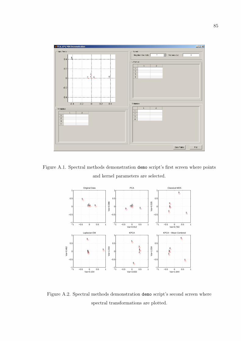
85

Figure A.1. Spectral methods demonstration demo script’s first screen where points

and kernel parameters are selected.

−1 −0.5 0 0.5 1−1

−0.5

0

0.5

1Original Data

123 4

5

6

−1 −0.5 0 0.5 1−1

−0.5

0

0.5

1PCA

Var=0.912

Var

=0.

088

1234

56

−1 −0.5 0 0.5 1−1

−0.5

0

0.5

1Laplacian EM

Var=0.154

Var

=0.

462

1234 5

6

−1 −0.5 0 0.5 1−1

−0.5

0

0.5

1Classical MDS

Var=0.763

Var

=0.

535

12

3

4

5

6

−1 −0.5 0 0.5 1−1

−0.5

0

0.5

1KPCA

Var=3.833

Var

=1.

034

123

4

5

6

−1 −0.5 0 0.5 1−1

−0.5

0

0.5

1KPCA − Mean Centered

Var=1.644

Var

=1.

034

123

4

5

6

Figure A.2. Spectral methods demonstration demo script’s second screen where

spectral transformations are plotted.

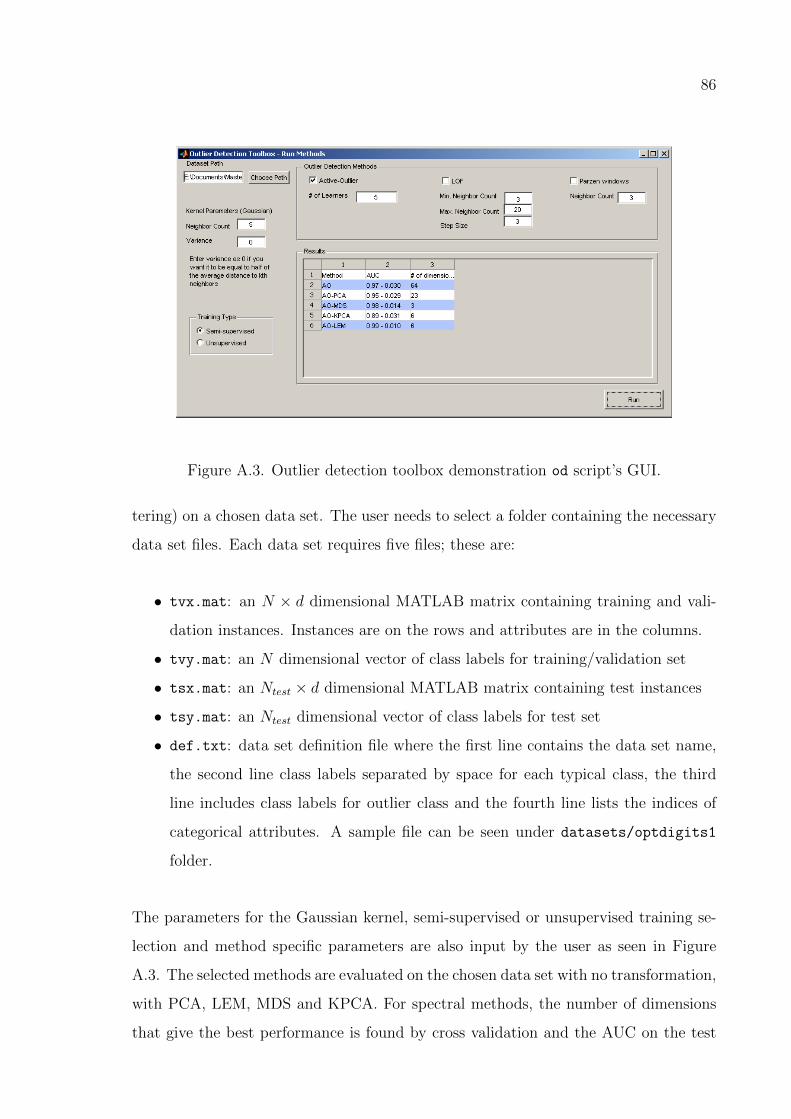
86

Figure A.3. Outlier detection toolbox demonstration od script’s GUI.

tering) on a chosen data set. The user needs to select a folder containing the necessary

data set files. Each data set requires five files; these are:

• tvx.mat: an N × d dimensional MATLAB matrix containing training and vali-

dation instances. Instances are on the rows and attributes are in the columns.

• tvy.mat: an N dimensional vector of class labels for training/validation set

• tsx.mat: an Ntest × d dimensional MATLAB matrix containing test instances

• tsy.mat: an Ntest dimensional vector of class labels for test set

• def.txt: data set definition file where the first line contains the data set name,

the second line class labels separated by space for each typical class, the third

line includes class labels for outlier class and the fourth line lists the indices of

categorical attributes. A sample file can be seen under datasets/optdigits1

folder.

The parameters for the Gaussian kernel, semi-supervised or unsupervised training se-

lection and method specific parameters are also input by the user as seen in Figure

A.3. The selected methods are evaluated on the chosen data set with no transformation,

with PCA, LEM, MDS and KPCA. For spectral methods, the number of dimensions

that give the best performance is found by cross validation and the AUC on the test

87

set is calculated with this dimensionality. The results are given in the GUI when the

run completes. Additionally, the MATLAB structures containing the results for each

run and ROC/PR curve plots are saved into the data set folder. An extra script to

od.m, od script.m, is also provided that shows how to run experiments with different

methods and parameters. odToolbox is distributed under the GNU General Public Li-

cense. It can be redistributed and modified freely for non-commercial use. We kindly

request users of this toolbox to reference this thesis in their publications.

88

REFERENCES

1. Alpaydın, E., Introduction to Machine Learning , MIT Press, Cambridge, MA,

USA, 2004.

2. Grubbs, F. E., “Procedures for Detecting Outlying Observations in Samples”, Tech-

nometrics , Vol. 11, No. 1, pp. 1–21, 1969.

3. Chandola, V., A. Banerjee and V. Kumar, “Anomaly Detection: A Survey”, ACM

Computing Surveys , Vol. 41, pp. 15:1–15:58, 2009.

4. Minsky, M., The Society of Mind , Simon and Schuster, New York, NY, USA, 1986.

5. Augusteijn, M. F. and B. A. Folkert, “Neural Network Classification and Novelty

Detection”, International Journal of Remote Sensing , Vol. 23, No. 14, pp. 2891–

2902, 2002.

6. Cun, L., B. Boser, J. S. Denker, D. Henderson, R. E. Howard, W. Hubbard and

L. D. Jackel, “Handwritten Digit Recognition with a Back-Propagation Network”,

Advances in Neural Information Processing Systems , pp. 396–404, 1990.

7. Hwang, B. and S. Cho, “Characteristics of Auto-associative MLP as a Novelty

Detector”, International Joint Conference on Neural Networks , Vol. 5, pp. 3086–

3091, 1999.

8. Dasgupta, D. and F. Nino, “A Comparison of Negative and Positive Selection Al-

gorithms in Novel Pattern Detection”, IEEE International Conference on Systems,

Man, and Cybernetics , Vol. 1, pp. 125 –130, 2000.

9. Albrecht, S., J. Busch, M. Kloppenburg, F. Metze and P. Tavan, “Generalized

Radial Basis Function Networks for Classification and Novelty Detection: Self-

organization of Optimal Bayesian Decision”, Neural Networks , Vol. 13, No. 10, pp.

89

1075 – 1093, 2000.

10. Fan, W., M. Miller, S. J. Stolfo and W. Lee, “Using Artificial Anomalies to De-

tect Unknown and Known Network Intrusions”, Proceedings of the First IEEE

International Conference on Data Mining , pp. 123–130, 2001.

11. Ratsch, G., S. Mika, B. Scholkopf and K.-R. Muller, “Constructing Boosting Algo-

rithms from SVMs: An Application to One-Class Classification”, IEEE Transac-

tions on Pattern Analysis and Machine Intelligence, Vol. 24, No. 9, pp. 1184–1199,

2002.

12. Scholkopf, B., J. C. Platt, J. C. Shawe-Taylor, A. J. Smola and R. C. Williamson,

“Estimating the Support of a High-Dimensional Distribution”, Neural Computa-

tion, Vol. 13, No. 7, pp. 1443–1471, 2001.

13. Roth, V., “Kernel Fisher Discriminants for Outlier Detection”, Neural Computa-

tion, Vol. 18, No. 4, pp. 942–960, 2006.

14. Parzen, E., “On Estimation of a Probability Density Function and Mode”, The

Annals of Mathematical Statistics , Vol. 33, No. 3, pp. 1065–1076, 1962.

15. Laurikkala, J., M. Juhola and E. Kentala, “Informal Identification of Outliers in

Medical Data”, The Fifth International Workshop on Intelligent Data Analysis in

Medicine and Pharmacology , pp. 17–29, 2000.

16. Ye, N. and Q. Chen, “An Anomaly Detection Technique Based on a Chi-square

Statistic for Detecting Intrusions into Information Systems”, Quality and Reliabil-

ity Engineering International , Vol. 17, No. 2, pp. 105–112, 2001.

17. Rousseeuw, P. J. and A. M. Leroy, Robust Regression and Outlier Detection, John

Wiley & Sons, Inc., New York, NY, USA, 1987.

18. Eskin, E., “Anomaly Detection over Noisy Data Using Learned Probability Distri-

90

butions”, Proceedings of the International Conference on Machine Learning , pp.

255–262, 2000.

19. Abraham, B. and G. E. P. Box, “Bayesian Analysis of Some Outlier Problems in

Time Series”, Biometrika, Vol. 66, No. 2, pp. 229–236, 1979.

20. Eskin, E., “Modeling System Calls for Intrusion Detection with Dynamic Window

Sizes”, Proceedings of DARPA Information Survivabilty Conference and Exposition

II (DISCEX), pp. 143–152, 2001.

21. Desforges, M. J., P. J. Jacob and J. E. Cooper, “Applications of Probability Density

Estimation to the Detection of Abnormal Conditions in Engineering”, Proceedings

of the Institution of Mechanical Engineers, Part C: Journal of Mechanical Engi-

neering Science, Vol. 212, No. 8, pp. 687–703, 1998.

22. Yu, J. X., W. Qian, H. Lu and A. Zhou, “Finding Centric Local Outliers in Cat-

egorical/Numerical Spaces”, Knowledge Information Systems , Vol. 9, No. 3, pp.

309–338, 2006.

23. He, Z., X. Xu and S. Deng, “Discovering Cluster-based Local Outliers”, Pattern

Recognition Letters , Vol. 24, No. 9-10, pp. 1641–1650, 2003.

24. Byers, S. and A. E. Raftery, “Nearest-Neighbor Clutter Removal for Estimating

Features in Spatial Point Processes”, Journal of the American Statistical Associa-

tion, Vol. 93, No. 442, pp. 577–584, 1998.

25. Eskin, E., A. Arnold, M. Prerau, L. Portnoy and S. Stolfo, “A Geometric Frame-

work for Unsupervised Anomaly Detection: Detecting Intrusions in Unlabeled

Data”, Applications of Data Mining in Computer Security , pp. 319–330, 2002.

26. Knorr, E. M., R. T. Ng and V. Tucakov, “Distance-based Outliers: Algorithms

and Applications”, The International Journal on Very Large Data Bases , Vol. 8,

No. 3-4, pp. 237–253, 2000.

91

27. Breunig, M. M., H. P. Kriegel, R. T. Ng and J. Sander, “LOF: Identifying Density-

based Local Outliers”, SIGMOD Record , Vol. 29, pp. 93–104, 2000.

28. Abe, N., B. Zadrozny and J. Langford, “Outlier Detection by Active Learning”,

Proceedings of the 12th ACM SIGKDD International Conference on Knowledge

Discovery and Data Mining , pp. 504–509, 2006.

29. Freund, Y. and R. E. Schapire, “A Decision-theoretic Generalization of Online

Learning and An Application to Boosting”, Proceedings of the Second European

Conference on Computational Learning Theory , pp. 23–37, 1995.

30. Breiman, L., “Bagging Predictors”, Machine Learning , Vol. 24, pp. 123–140, 1996.

31. Breiman, L., “Random Forests”, Machine Learning , Vol. 45, No. 1, pp. 5–32, 2001.

32. Lazarevic, A. and V. Kumar, “Feature Bagging for Outlier Detection”, Proceedings

of the Eleventh ACM SIGKDD International Conference on Knowledge Discovery

in Data Mining , pp. 157–166, 2005.

33. Vapnik, V., The Nature of Statistical Learning Theory , Springer, New York, NY,

USA, 2000.

34. L.K. Saul, J. H. H. F. S., K.Q. Weinberger and D. D. Lee, “Spectral methods for

dimensionality reduction”, Semi-Supervised Learning , pp. 293–300, 2006.

35. Eckart, C. and G. Young, “The Approximation of One Matrix by Another of Lower

Rank”, Psychometrika, Vol. 1, pp. 211–218, 1936.

36. Saad, Y., Numerical Methods for Large Eigenvalue Problems , Halstead Press, New

York, NY, USA, 1992.

37. Jolliffe, I., Principal Component Analysis , Springer-Verlag, New York, NY, USA,

2002.

92

38. Scholkopf, B., A. J. Smola and K.-R. Muller, “Kernel Principal Component Anal-

ysis”, International Conference on Artificial Neural Networks , pp. 583–588, 1997.

39. Scholkopf, B., A. J. Smola and K.-R. Muller, “Nonlinear Component Analysis as a

Kernel Eigenvalue Problem”, Neural Computation, Vol. 10, No. 5, pp. 1299–1319,

1998.

40. Cox, T. and M. Cox, Multidimensional Scaling , Chapman & Hall, London, UK,

1994.

41. Belkin, M. and P. Niyogi, “Laplacian Eigenmaps for Dimensionality Reduction and

Data Representation”, Neural Computation, Vol. 15, No. 6, pp. 1373–1396, 2003.

42. Shyu, M.-L., S.-C. Chen, K. Sarinnapakorn and L. Chang, “A Novel Anomaly

Detection Scheme Based on Principal Component Classifier”, Proceedings of the

IEEE Foundations and New Directions of Data Mining Workshop, in Conjunction

with the Third IEEE International Conference on Data Mining (ICDM’03), pp.

172–179, 2003.

43. Wang, W., X. Guan and X. Zhang, “A Novel Intrusion Detection Method Based

on Principal Component Analysis”, Advances in Neural Networks, International

IEEE Symposium on Neural Networks , pp. 657–662, 2004.

44. Parra, L., G. Deco and S. Miesbach, “Statistical Independence and Novelty Detec-

tion with Information Preserving Nonlinear Maps”, Neural Computation, Vol. 8,

pp. 260–269, 1995.

45. Dutta, H., C. Giannella, K. D. Borne and H. Kargupta, “Distributed Top-K Outlier

Detection from Astronomy Catalogs Using the DEMAC System.”, SIAM Interna-

tional Conference on Data Mining , pp. 110–121, 2007.

46. Salzberg, S. L., “C4.5: Programs for Machine Learning”, Machine Learning ,

Vol. 16, pp. 235–240, 1994.

93

47. Chang, C.-C. and C.-J. Lin, “LIBSVM: A Library For Support Vector Machines”,

ACM Transactions on Intelligent Systems and Technology , Vol. 2, No. 3, pp. 27:1–

27:27, 2011.

48. Frank, A. and A. Asuncion, UCI Machine Learning Repository , 2010,

http://archive.ics.uci.edu/ml, 10.09.2011.

49. Friedman, M., “The Use of Ranks to Avoid the Assumption of Normality Implicit in

the Analysis of Variance”, Journal of the American Statistical Association, Vol. 32,

No. 200, pp. 675–701, 1937.

50. Alpaydın, E., “Combined 5×2 Cv F Test for Comparing Supervised Classification

Learning Algorithms.”, Neural Computation, Vol. 11, No. 8, pp. 1885–1892, 1999.

51. Nemenyi, P. B., Distribution-free Multiple Comparisons , Ph.D. Thesis, Princeton

University, 1963.

52. MIT Center For Biological and Computation Learning, CBCL Face Database, 2000,

http://cbcl.mit.edu/software-datasets/FaceData2.html, 15.01.2012.

53. Roweis, S. T. and L. K. Saul, “Nonlinear Dimensionality Reduction by Locally

Linear Embedding”, Science, Vol. 290, No. 5500, pp. 2323–2326, 2000.

54. Tenenbaum, J. B., V. d. Silva and J. C. Langford, “A Global Geometric Framework

for Nonlinear Dimensionality Reduction”, Science, Vol. 290, No. 5500, pp. 2319–

2323, 2000.