1

Spectral Method for Phase Retrieval: an ExpectationPropagation Perspective

Junjie Ma, Rishabh Dudeja, Ji Xu, Arian Maleki, Xiaodong Wang

Abstract—Phase retrieval refers to the problem of recoveringa signal x? ∈ Cn from its phaseless measurements yi = |aH

i x?|,where {ai}mi=1 are the measurement vectors. Spectral method iswidely used for initialization in many phase retrieval algorithms.The quality of spectral initialization can have a major impacton the overall algorithm. In this paper, we focus on the modelwhere A = [a1, . . . ,am]H has orthonormal columns, and studythe spectral initialization under the asymptotic setting m,n→ ∞with m/n → δ ∈ (1,∞). We use the expectation propagationframework to characterize the performance of spectral initializa-tion for Haar distributed matrices. Our numerical results confirmthat the predictions of the EP method are accurate for not-onlyHaar distributed matrices, but also for realistic Fourier basedmodels (e.g. the coded diffraction model). The main findings ofthis paper are the following:• There exists a threshold on δ (denoted as δweak) below which

the spectral method cannot produce a meaningful estimate.We show that δweak = 2 for the column-orthonormal model.In contrast, previous results by Mondelli and Montanarishow that δweak = 1 for the i.i.d. Gaussian model.

• The optimal design for the spectral method coincides withthat for the i.i.d. Gaussian model, where the latter wasrecently introduced by Luo, Alghamdi and Lu.

Index Terms—Phase retrieval, spectral method, coded diffrac-tion pattern, expectation propagation (EP), approximate messagepassing (AMP), state evolution, orthogonal AMP, vector AMP.

I. INTRODUCTION

In many scientific and engineering applications, it is expen-sive or even impossible to measure the phase of a signal dueto physical limitations [1]. Phase retrieval refers to algorith-mic methods for reconstructing signals from magnitude-onlymeasurements. The measuring process for the phase retrievalproblem can be modeled as

yi = |(Ax?)i| , i = 1, 2 . . . ,m, (1)

where A ∈ Cm×n (m > n) is the measurement matrix,x? ∈ Cn×1 is the signal to be recovered, and (Ax?)i denotes

This work was supported in part by National Science Foundation (NSF)under grant CCF 1814803 and Office of Naval Research (ONR) under grantN000141712827.

J. Ma was with the Department of Statistics and the Department of ElectricalEngineering of Columbia University, New York, USA. He is now with theInstitute of Computational Mathematics and Scientific/Engineering Comput-ing, Academy of Mathematics and Systems Science, Chinese Academy ofSciences, Beijing, China. (e-mail:majunjie@lsec.cc.ac.cn)

R. Dudeja and Arian Maleki are with the Department of Statistics,Columbia University, New York, USA. (e-mail: rd2714@columbia.edu; ar-ian@stat.columbia.edu)

J. Xu is with the Department of Computer Science, Columbia University,New York, USA. (e-mail: jixu@cs.columbia.edu)

X. Wang is with the Department of Electrical Engineering, ColumbiaUniversity, New York, USA. (e-mail: xw2008@columbia.edu)

the ith entry of the vector Ax?. Phase retrieval has importantapplications in areas ranging from X-ray crystallography,astronomical imaging, and many others [1].

Phase retrieval has attracted a lot of research interests sincethe work of Candes et al [2], where it is proved that a convexoptimization based algorithm can provably recover the signalunder certain randomness assumptions on A. However, thehigh computational complexity of the PhaseLift algorithm in[2] prohibits its practical applications. More recently, a lotof algorithms were proposed as low-cost iterative solvers forthe following nonconvex optimization problem (or its variants)[3]–[6]:

argminx∈Cm

1

m

m∑i=1

(|yi|2 − |(Ax)i|2

)2. (2)

These algorithms typically initialize their estimates using aspectral method [7] and then refine the estimates via alternativeminimization [7], gradient descend (and variants) [3]–[6] orapproximate message passing [8]. Since the problem in (2) isnonconvex, the initialization step plays a crucial role for manyof these algorithms.

Spectral methods are widely used for initializing localsearch algorithms in many signal processing applications. Inthe context of phase retrieval, spectral initialization was firstproposed in [7] and later studied in [4], [5], [9]–[12]. To bespecific, a spectral initial estimate is given by the leadingeigenvector (after proper scaling) of the following data matrix[10]:

D∆= AHdiag{T (y1), . . . , T (ym)}A, (3)

where diag{a1, . . . , am} denotes a diagonal matrix formed by{ai}mi=1 and T : R+ 7→ R is a nonlinear processing function.A natural measure of the quality of the spectral initializationis the cosine similarity [10] between the estimate and the truesignal vector:

P 2T (x?, x)

∆=

|xH? x|2

‖x?‖2‖x‖2, (4)

where x denotes the spectral estimate. The performance ofthe spectral initialization highly depends on the processingfunction T . Popular choices of T include the “trimming”function Ttrim proposed in [4] (the name follows [10]), the“subset method” in [5], TMM(y) proposed by Mondelli and

arX

iv:1

903.

0250

5v2

[cs

.IT

] 9

Sep

202

0

2

Montanari in [11], and T? recently proposed in [12]:

Ttrim(y) = δy2 · I(δy2 < c22), (5a)

Tsubset(y) = I(δy2 > c1), (5b)

TMM(y) = 1−√δ

δy2 +√δ − 1

, (5c)

T?(y) = 1− 1

δy2. (5d)

In the above expressions, c1 > 0 and c2 > 0 are tunablethresholds, and I(·) denotes an indicator function that equalsone when the condition is satisfied and zero otherwise.

The asymptotic performance of the spectral method wasstudied in [10] under the assumption that A contains i.i.d.Gaussian entries. The results of [10] unveil a phase tran-sition phenomenon in the regime where m,n → ∞ withm/n = δ ∈ (0,∞) fixed. Specifically, there exists a thresholdon the measurement ratio δ: below this threshold the cosinesimilarity P 2

T (x,x?) converges to zero (meaning that x isnot a meaningful estimate) and above it P 2

T (x,x?) is strictlypositive. Later, Mondelli and Montanari showed in [11] thatTMM defined in (5) minimizes the above-mentioned recon-struction threshold. Following [11], we will call the minimumthreshold (over all possible T ) the weak threshold. It is provedin [11] that the weak thresholds are 0.5 and 1, respectively,for real and complex valued models. Further, [11] showed thatthese thresholds are also information-theoretically optimal forweak recovery. Notice that TMM minimizes the reconstructionthreshold, but does not necessarily maximize P 2

T (x,x?) whenδ is larger than the weak threshold. The latter criterion ismore relevant in practice, since intuitively speaking a largerP 2T (x,x?) implies better initialization, and hence the overall

algorithm is more likely to succeed. This problem was recentlystudied by Luo, Alghamdi and Lu in [12], where it wasshown that the function T? defined in (5) uniformly maximizesP 2T (x,x?) for an arbitrary δ (and hence also achieves the weak

threshold).Notice that the analyses of the spectral method in [10]–

[12] are based on the assumption that A has i.i.d. Gaussianelements. This assumption is key to the random matrix theory(RMT) tools used in [10]. However, the measurement matrixA for many (if not all) important phase retrieval applicationsis a Fourier matrix [13]. In certain applications, it is possible torandomize the measuring mechanism by adding random masks[14]. Such models are usually referred to as coded diffractionpatterns (CDP) models [14]. In the CDP model, A can beexpressed as

A =

FP1

FP2

. . .FPL

, (6)

where F n×n is a square discrete Fourier transform (DFT)matrix, and Pl = diag{ejθl,1 , . . . , ejθl,n} represents the effectof random masks. For the CDP model, A has orthonormalcolumns, namely,

AHA = I. (7)

In this paper, we assume A to be an isotropically randomunitary matrix (or simply Haar distributed). We study the

performance of the spectral method and derive a formula topredict the cosine similarity ρ2

T (x,x?). We conjecture thatour prediction is asymptotically exact as m,n → ∞ withm/n = δ ∈ (1,∞) fixed. Based on this conjecture, we areable to show the following.• There exists a threshold on δ (denoted as δweak) below

which the spectral method cannot produce a meaningfulestimate. We show that δweak = 2 for the column-orthonormal model. In contrast, previous results by Mon-delli and Montanari show that δweak = 1 for the i.i.d.Gaussian model.

• The optimal design for the spectral method coincides withthat for the i.i.d. Gaussian model, where the latter wasrecently derived by Luo, Alghamdi and Lu.

Our asymptotic predictions are derived by analyzing anexpectation propagation (EP) [15] type message passing algo-rithm [16], [17] that aims to find the leading eigenvector. A keytool in our analysis is a state evolution (SE) technique that hasbeen extensively studied for the compressed sensing problem[17]–[22]. Several arguments about the connection betweenthe message passing algorithm and the spectral estimator isheuristic, and thus the results in this paper are not rigorousyet. Nevertheless, numerical results suggest that our analysisaccurately predicts the actual performance of the spectralinitialization under the practical CDP model. This is perhaps asurprising phenomenon, considering the fact that the sensingmatrix in (6) is still quite structured although the matrices{Pl} introduce certain randomness.

We point out that the predictions of this paper have beenrigorously proved using RMT tools in [23]. It is also expectedthat the same results can be obtained by using the replicamethod [24]–[26], which is a non-rigorous, but powerful toolfrom statistical physics. Compared with the replica method,our method seems to be technically simpler and more flexible(e.g., we might be able to handle the case where the signal isknown to be positive).

Finally, it should be noted that although the coded diffrac-tion pattern model is much more practical than the i.i.d.Gaussian model, it is still far from practical for some importantphase retrieval applications (e.g., X-ray crystallography). Aspointed out in [27], [28], designing random masks for X-raycrystallography would correspond to manipulating the masksat sub-nanometer resolution and thus physically infeasible. Onthe other hand, it has been suggested to use multiple illumina-tions for certain types of imaging applications (see [29, Section2.3] for discussions and related references). We emphasize thatthe results in this paper only apply to (empirically) the random-masked Fourier model, and the theory for the challenging non-random Fourier case is still open.

Notations: a∗ denotes the conjugate of a complex num-ber a. We use bold lower-case and upper case letters forvectors and matrices respectively. For a matrix A, AT andAH denote the transpose of a matrix and its Hermitianrespectively. diag{a1, a2, . . . , an} denotes a diagonal matrixwith {ai}ni=1 being the diagonal entries. x ∼ CN (0, σ2I)is circularly-symmetric Gaussian if Re(x) ∼ N (0, σ2/2I),Im(x) ∼ N (0, σ2/2I), and Re(x) is independent of Im(x).For a, b ∈ Cm, define 〈a, b〉 =

∑mi=1 a

∗i bi. For a Hermitian

3

matrix H ∈ Cn×n, λ1(H) and λn(H) denote the largest andsmallest eigenvalues of H respectively. For a non-Hermitianmatrix Q, λ1(Q) denotes the eigenvalue of Q that has thelargest magnitude. Tr(·) denotes the trace of a matrix. P→denotes convergence in probability.

II. ASYMPTOTIC ANALYSIS OF THE SPECTRAL METHOD

This section presents the main results of this paper. Ourresults have not been fully proved, we call them “claims”throughout this section to avoid confusion. The rationales forour claims will be discussed in Section IV.

A. Assumptions

In this paper, we make the following assumption on thesensing matrix A.

Assumption 1. The sensing matrix A ∈ Cm×n (m > n)is sampled uniformly at random from column orthogonalmatrices satisfying AHA = I .

Assumption 1 introduces certain randomness assumptionabout the measurement matrix A. However, in practice, themeasurement matrix is usually a Fourier matrix or somevariants of it. One particular example is the coded diffractionpatterns (CDP) model in (6). For this model, the only freedomone has is the “random masks” {Pl}, and the overall matrixis still quite structured. In this regard, it is perhaps quitesurprising that the predictions developed under Assumption1 are very accurate even for the CDP model. Please refer toSection V for our numerical results.

We further make the following assumption about the pro-cessing function T : R+ 7→ R.

Assumption 2. The processing function T : R+ 7→ R satisfiessupy≥0 T (y) = Tmax, where Tmax <∞.

As pointed out in [10], the boundedness of T in Assumption2-(I) is the key to the success of the truncated spectralinitializer proposed in [4]. (Following [10], we will call itthe trimming method in this paper.) Notice that we assumeTmax = 1 without any loss of generality. To see this, considerthe following modification of T :

T (y)∆=C + T (y)

C + Tmax,

where C > max{0,−Tmax}. It is easy to see that

AHdiag{T (y1), . . . , T (ym)}A

=C

C + TmaxI +

1

C + TmaxAHTA,

where we used AHA = I . Clearly, the top eigenvector ofAHTA is the same as that of AHdiag{T (y1), . . . , T (ym)}A,where for the latter matrix we have supy≥0 T (y) = 1.

B. Asymptotic analysis

Let x be the principal eigenvector of the following datamatrix:

D∆= AHTA, (8)

where T = diag{T (y1), . . . , T (ym)}. Following [10], we usethe squared cosine similarity defined below to measure theaccuracy of x:

P 2T (x,x?)

∆=

|xH? x|2

‖x?‖2‖x‖2. (9)

Our goal is to understand how P 2T (x,x?) behaves when

m,n → ∞ with a fixed ratio m/n = δ. It seems possibleto solve this problem by adapting the tools developed in [10].Yet, we take a different approach which we believe to be tech-nically simpler and more flexible. Specifically, we will derivea message passing algorithm to find the leading eigenvectorof the data matrix. Central to our analysis is a deterministicrecursion, called state evolution (SE), that characterizes theasymptotic behavior of the message passing algorithm. Byanalyzing the stationary points of the SE, we obtain certainpredictions about the spectral estimator. This approach hasbeen adopted in [30] to analyze the asymptotic performanceof the LASSO estimator and in [31] for the nonnegative PCAestimator, based on the approximate message passing (AMP)algorithm [32], [33]. However, the SE analysis of AMP doesnot apply to the partial orthogonal matrix model consideredin this paper.

Different from [31], our analysis is based on a variant ofthe expectation propagation (EP) algorithm [15], [16], calledPCA-EP in this paper. Different from AMP, such EP-stylealgorithms could be analyzed via SE for a wider class ofmeasurement matrices, including the Haar model consideredhere [17]–[22], [34], [35]. The derivations of PCA-EP and itsSE analysis will be introduced in Section IV.

Our characterization of P 2T (x,x?) involves the following

functions (for µ ∈ (0, 1]):

ψ1(µ)∆=

E[δ|Z?|2G

]E[G]

,

ψ2(µ)∆=

E[G2]

(E[G])2 ,

ψ3(µ)∆=

√E [δ|Z?|2G2]

E[G],

(10)

where Z? ∼ CN (0, 1/δ) and G is a shorthand for

G(|Z?|, µ)∆=

1

1/µ− T (|Z?|). (11)

We note that ψ1, ψ2 and ψ3 all depend on the processingfunction T . However, to simplify notation, we will not makethis dependency explicit. Claim 1 below summarizes ourasymptotic characterization of the cosine similarity P 2

T (x,x?).

Claim 1 (Cosine similarity). Define

ρ2T (µ, δ)

∆=

(δδ−1

)2

− δδ−1 · ψ2(µ)

ψ23(µ)− δ

δ−1 · ψ2(µ), (12)

and

Λ(µ)∆=

1

µ− δ − 1

δ· 1

E[G(|Z?|, µ)], (13)

4

where Z? ∼ CN (0, 1/δ). Let

µ(δ)∆= argmin

µ∈(0,1]

Λ(µ). (14)

Then, as m,n→∞ with a fixed ratio m/n = δ > 1, we have

limm→∞

P 2T (x,x?)

P→ ρ2T (δ), (15)

where with a slight abuse of notations,

ρ2T (δ)

∆=

{ρ2T(µ(δ), δ

), if ψ1 (µ(δ)) ≥ δ

δ−1 ,

0 if ψ1 (µ(δ)) < δδ−1 ,

(16)

and µ(δ) is a solution to

ψ1(µ) =δ

δ − 1, µ ∈ (0, µ(δ)]. (17)

Claim 1, which is reminiscent of Theorem 1 in [10], revealsa phase transition behavior of P 2

T (x,x?): P 2T (x,x?) is strictly

positive when ψ1(µ(δ)) > δδ−1 and is zero otherwise. In the

former case, the spectral estimator is positively correlated withthe true signal and hence provides useful information aboutx?; whereas in the latter case P 2

T (x,x?) → 0, meaning thatthe spectral estimator is asymptotically orthogonal to the truesignal and hence performs no better than a random guess.Claim 1 is derived from the analysis of an EP algorithm whosefixed points correspond to the eigenvector of the matrix D.The main difficulty for making this approach rigorous is toprove the EP estimate converges to the leading eigenvector.Currently, we do not have a proof yet, but we will providesome heuristic arguments in Section IV.

Remark 1. For notational simplicity, we will write µ(δ) andµ(δ) as µ and µ, respectively.

Some remarks about the phase transition condition are givenin Lemma 1 below. Item (i) guarantees the uniqueness of thesolution to (17). Item (ii) is the actual intuition that leads to theconjectured phase transition condition. The proof of Lemma1 can be found in Appendix A.

Lemma 1. (i) Eq. (17) has a unique solution if ψ1 (µ) > δδ−1 ,

where µ is defined in (14). (ii) ψ1 (µ) > δδ−1 if and only if

there exists a µ ∈ (0, 1] such that

ψ1(µ) =δ

δ − 1and 0 < ρ2

T (µ, δ) < 1.

The latter statement is equivalent to

ψ1(µ) =δ

δ − 1and ψ2(µ) <

δ

δ − 1.

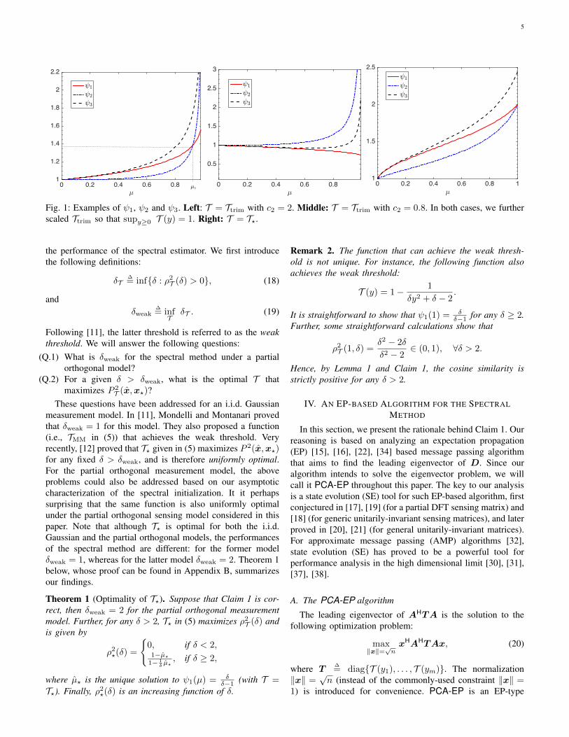
Fig. 1 plots ψ1, ψ2 and ψ3 for various choices of T . Thefirst two subfigures employ the trimming function Ttrim in (5a)(with different truncation thresholds), and third subfigure usesthe function T? in (5d).

Notice that for the first and third subfigures of Fig. 1, ψ1 andψ2 have unique nonzero crossing points in µ ∈ (0, 1], whichwe denote as µ�. Further, ψ1 > ψ2 for µ < µ�, and ψ1 < ψ2

for µ > µ� (for the first subfigure). Then by Lemma 1-(ii), aphase transition happens when ψ1(µ�) > δ

δ−1 , or equivalently

δ >ψ1(µ�)

ψ1(µ�)− 1

∆= δT .

The spectral estimator is positively correlated with the signalwhen δ > δT , and perpendicular to it otherwise.

Now consider the second subfigure of Fig. 1. Note that Tonly depends on δ through δy2, and it is straightforward tocheck that ψ1, ψ2 and ψ3 do not depend on δ for such T .Hence, there is no solution to ψ1(µ) = δ

δ−1 for any δ ∈ [1,∞).According to Lemma 1 and Claim 1, we have P 2

T (x,x?)→ 0.The situation for T? is shown in the figure on the right panelof Fig. 1.

C. Discussions

The main finding of this paper (namely, Claim 1) is acharacterization of the asymptotic behavior of the spectralmethod. As will be explained in Section IV, the intuition forClaim 1 is that the fixed point of an expectation-propagationtype algorithm (called PCA-EP in this paper) coincides withan eigenvector with a particular eigenvalue (see Lemma 2) ofthe data matrix which the spectral estimator uses. Furthermore,the asymptotic behavior PCA-EP could be conveniently an-alyzed via the state evolution (SE) platform. This motivatesus to study the spectral estimator by studying the fixedpoint of PCA-EP. The difficulty here is to prove that thestationary points of the PCA-EP converge to the eigenvectorcorresponding to the largest eigenvalue. Currently, we do nothave a rigorous proof for Claim 1.

We would like to mention two closely-related work [30],[36] where the approximate message passing (AMP) algorithmand the state evolution formalism was employed to study thehigh-dimensional asymptotics of the LASSO problem and thenonnegative PCA problem respectively. Unfortunately, neitherapproach is applicable to our problem. In [30], the convexityof the LASSO problem is crucial to prove that the AMPestimate converges to the minimum of the LASSO problem. Incontrast, the variational formulation of the eigenvalue problemis nonconvex. In [36], the authors used a Gaussian comparisoninequalities to upper bound the cosine similarity between thesignal vector and the PCA solution and use the AMP estimatesto lower bound the same quantity, and combining the lowerand upper bound yields the desired result. For our problem,however, the sensing matrix is not Gaussian and the Gaussiancomparison inequality is not immediately applicable.

Although we do not have a rigorous proof for Claim 1 yet,we will present some heuristic arguments in Section IV-D.Our main heuristic arguments for Claim 1 is Lemma 3 andLemma 4, which establishes a connection between the extremeeigenvalues of the original matrix D (see (3)) and the matrixE(µ) (see definition in (21a)) that originates from the PCA-EP algorithm. These two lemmas provide some interestingobservations that might shed light on Claim 1. The detaileddiscussions can be found in Section IV-D.

III. OPTIMAL DESIGN OF T

Claim 1 characterizes the condition under which the leadingeigenvector x is positively correlated with the signal vector x?for a given T . We would like to understand how does T affect

5

70 0.2 0.4 0.6 0.81

1.2

1.4

1.6

1.8

2

2.2

A1

A2

A3

7&7

0 0.2 0.4 0.6 0.8

0.5

1

1.5

2

2.5

3

A1

A2

A3

70 0.2 0.4 0.6 0.8 11

1.5

2

2.5A1

A2

A3

Fig. 1: Examples of ψ1, ψ2 and ψ3. Left: T = Ttrim with c2 = 2. Middle: T = Ttrim with c2 = 0.8. In both cases, we furtherscaled Ttrim so that supy≥0 T (y) = 1. Right: T = T?.

the performance of the spectral estimator. We first introducethe following definitions:

δT∆= inf{δ : ρ2

T (δ) > 0}, (18)

andδweak

∆= infT

δT . (19)

Following [11], the latter threshold is referred to as the weakthreshold. We will answer the following questions:

(Q.1) What is δweak for the spectral method under a partialorthogonal model?

(Q.2) For a given δ > δweak, what is the optimal T thatmaximizes P 2

T (x,x?)?These questions have been addressed for an i.i.d. Gaussian

measurement model. In [11], Mondelli and Montanari provedthat δweak = 1 for this model. They also proposed a function(i.e., TMM in (5)) that achieves the weak threshold. Veryrecently, [12] proved that T? given in (5) maximizes P 2(x,x?)for any fixed δ > δweak, and is therefore uniformly optimal.For the partial orthogonal measurement model, the aboveproblems could also be addressed based on our asymptoticcharacterization of the spectral initialization. It it perhapssurprising that the same function is also uniformly optimalunder the partial orthogonal sensing model considered in thispaper. Note that although T? is optimal for both the i.i.d.Gaussian and the partial orthogonal models, the performancesof the spectral method are different: for the former modelδweak = 1, whereas for the latter model δweak = 2. Theorem 1below, whose proof can be found in Appendix B, summarizesour findings.

Theorem 1 (Optimality of T?). Suppose that Claim 1 is cor-rect, then δweak = 2 for the partial orthogonal measurementmodel. Further, for any δ > 2, T? in (5) maximizes ρ2

T (δ) andis given by

ρ2?(δ) =

{0, if δ < 2,1−µ?

1− 1δ µ?

, if δ ≥ 2,

where µ? is the unique solution to ψ1(µ) = δδ−1 (with T =

T?). Finally, ρ2?(δ) is an increasing function of δ.

Remark 2. The function that can achieve the weak thresh-old is not unique. For instance, the following function alsoachieves the weak threshold:

T (y) = 1− 1

δy2 + δ − 2.

It is straightforward to show that ψ1(1) = δδ−1 for any δ ≥ 2.

Further, some straightforward calculations show that

ρ2T (1, δ) =

δ2 − 2δ

δ2 − 2∈ (0, 1), ∀δ > 2.

Hence, by Lemma 1 and Claim 1, the cosine similarity isstrictly positive for any δ > 2.

IV. AN EP-BASED ALGORITHM FOR THE SPECTRALMETHOD

In this section, we present the rationale behind Claim 1. Ourreasoning is based on analyzing an expectation propagation(EP) [15], [16], [22], [34] based message passing algorithmthat aims to find the leading eigenvector of D. Since ouralgorithm intends to solve the eigenvector problem, we willcall it PCA-EP throughout this paper. The key to our analysisis a state evolution (SE) tool for such EP-based algorithm, firstconjectured in [17], [19] (for a partial DFT sensing matrix) and[18] (for generic unitarily-invariant sensing matrices), and laterproved in [20], [21] (for general unitarily-invariant matrices).For approximate message passing (AMP) algorithms [32],state evolution (SE) has proved to be a powerful tool forperformance analysis in the high dimensional limit [30], [31],[37], [38].

A. The PCA-EP algorithm

The leading eigenvector of AHTA is the solution to thefollowing optimization problem:

max‖x‖=√n

xHAHTAx, (20)

where T∆= diag{T (y1), . . . , T (ym)}. The normalization

‖x‖ =√n (instead of the commonly-used constraint ‖x‖ =

1) is introduced for convenience. PCA-EP is an EP-type

6

message passing algorithm that aims to solve (20). Startingfrom an initial estimate z0, PCA-EP proceeds as follows (fort ≥ 1):

PCA-EP : zt+1 =(δAAH − I

)( G

〈G〉− I

)︸ ︷︷ ︸

E(µ)

zt,

(21a)where G is a diagonal matrix defined as

G∆= diag

{1

µ−1 − T (y1), . . . ,

1

µ−1 − T (ym)

}, (21b)

and〈G〉 ∆

=1

mTr(G). (21c)

In (21b), µ ∈ (0, 1] is a parameter that can be tuned. At everyiteration of PCA-EP , the estimate for the leading eigenvectoris given by

xt+1 =

√n

‖AHzt+1‖·AHzt+1. (21d)

The derivations of PCA-EP can be found in Appendix C.Before we proceed, we would like to mention a couple ofpoints:• The PCA-EP algorithm is a tool for performance analy-

sis, not an actual numerical method for finding the leadingeigenvector. Further, our analysis is purely based on theiteration defined in (21), and the heuristic behind (21) isirrelevant for our analysis.

• The PCA-EP iteration has a parameter: µ ∈ (0, 1], whichdoes not change across iterations. To calibrate PCA-EPwith the eigenvector problem, we need to choose thevalue of µ carefully. We will discuss the details in SectionIV.

• From this representation, (21a) can be viewed as a powermethod applied to E(µ). This observation is crucial forour analysis. We used the notation E(µ) to emphasizethe impact of µ.

• The two matrices involved in E(µ) satisfy the following“zero-trace” property (referred to as “divergence-free” in[18]):

1

mTr

(G

〈G〉− I

)= 0 and

1

mTr(δAAH − I) = 0.

(22)This zero-trace property is the key to the correctness ofthe state evolution (SE) characterization.

B. State evolution analysis

State evolution (SE) was first introduced in [32], [33] toanalyze the dynamic behavior of AMP. However, the originalSE technique for AMP only works when the sensing matrixA has i.i.d. entries. Similar to AMP, PCA-EP can also bedescribed by certain SE recursions, but the SE for PCA-EP works for a wider class of sensing matrices (specifically,unitarily-invariant A [18], [20], [21]) that include the randompartial orthogonal matrix considered in this paper.

Denote z? = Ax?. Assume that the initial estimate z0 d=

α0z?+σ0w0, where w0 ∼ CN (0, 1/δI) is independent of z?.

Then, intuitively speaking, PCA-EP has an appealing propertythat zt+1 in (21a) is approximately

zt+1 ≈ αt+1z z? + σt+1wt+1, (23)

where αt and σt are the variables defined in (24), and wt+1 isan iid Gaussian vector. Due to this property, the distribution ofzt is fully specified by αt and σt. Further, for a given T anda fixed value of δ, the sequences {αt}t≥1 and {σ2

t }t≥1 canbe calculated recursively from the following two-dimensionalmap:

αt+1 = (δ − 1) · αt ·(ψ1(µ)− 1

), (24a)

σ2t+1 = (δ − 1) ·

[|αt|2 ·

(ψ2

3(µ)− ψ21(µ)

)+ σ2

t ·(ψ2(µ)− 1

)],

(24b)

where the functions ψ1, ψ2 and ψ3 are defined in (10). Togain some intuition on the SE, we present a heuristic way ofderiving the SE in Appendix D. The conditioning techniquedeveloped in [20], [21] is promising to prove Claim 2, butwe need to generalize the results to handle complex-valuednonlinear model with possibly non-continuous T . Given thefact that the connection between PCA-EP and the spectralestimator is already non-rigorous, we did not make such aneffort.

Claim 2 (SE prediction). Consider the PCA-EP algorithmin (21). Assume that the initial estimate z0 d

= α0z? + σ0w0

where w0 ∼ CN (0, 1/δI) is independent of z?. Then, almostsurely, the following hold for t ≥ 1:

limn→∞

〈z?, zt〉‖z?‖2

= αt and limn→∞

‖zt − αtz?‖2

‖z?‖2= σ2

t ,

where αt and σ2t are defined in (24). Furthermore, almost

surely we have

limn→∞

P 2T (xt,x) = lim

n→∞|〈x?,xt〉|2

‖x?‖2‖xt‖2=

|αt|2

|αt|2 + δ−1δ · σ

2t

,

(25)

where xt is defined in (21d).

C. Connection between PCA-EP and the PCA problem

Lemma 2 below shows that any nonzero stationary point ofPCA-EP in (21) is an eigenvector of the matrix D = AHTA.This is our motivation for analyzing the performance of thespectral method through PCA-EP.

Lemma 2. Consider the PCA-EP algorithm in (21) with µ ∈(0, 1]. Let z∞ be an arbitrary stationary point of PCA-EP .Suppose that AHz∞ 6= 0, then (x∞, λ(µ)) is an eigen-pairof D = AHTA, where the eigenvalue λ(µ) is given by

λ(µ) =1

µ− δ − 1

δ

1

〈G〉. (26)

Proof. We introduce the following auxiliary variable:

pt∆=

(G

〈G〉− I

)zt. (27)

When z∞ is a stationary point of (21a), we have

p∞ =

(1

〈G〉(1/µI − T )−1 − I

)(δAAH − I)p∞. (28)

7

Rearranging terms, we have(1

〈G〉(1/µI − T )−1

)p∞

=

(1

〈G〉(1/µI − T )−1 − I

)δAAHp∞.

Multiplying AH〈G〉(1/µI −T ) from both sides of the aboveequation yields

AHp∞ = AH (I − 〈G〉(1/µI − T )) δAAHp∞

= δ(1− µ−1〈G〉)AHp∞ + δ〈G〉 ·AHTAAHp∞.

After simple calculations, we finally obtain

AHTA(AHp∞

)=

(1

µ− δ − 1

δ

1

〈G〉

)(AHp∞

). (29)

In the above, we have identified an eigen-pair for the matrixAHTA. To complete our proof, we note from (21a) and (27)that z∞ = (δAAH − I)p∞ and so

AHz∞ = AH(δAAH − I)p∞

= (δ − 1)AHp∞.

Hence,

x∞∆=

√n

‖AHz∞‖·AHz∞ =

√n

‖AHp∞‖·AHp∞ (30)

is also an eigenvector.

Remark 3. Notice that the eigenvalue identified in (26) isclosely related to the function Λ(·) in (13). In fact, theonly difference between (26) and (13) is that the normal-ized trace 〈G〉 in (26) is replaced by E[G(|Z?|, µ)], whereZ? ∼ CN (0, 1/δ). Under certain mild regularity conditions onT , it is straightforward to use the weak law of large numbersto prove 〈G〉 p→ E[G(|Z?|, µ)].

Lemma 2 shows that the stationary points of the PCA-EPalgorithm are eigenvectors of AHTA. Since the asymptoticperformance of PCA-EP can be characterized via the SEplatform, it is conceivable that the fixed points of the SEdescribe the asymptotic performance of the spectral estimator.However, the answers to the following questions are stillunclear:• Even though x∞ is an eigenvector of AHTA, does it

correspond to the largest eigenvalue?• The eigenvalue in (26) depends on µ, which looks like a

free parameter. How should µ be chosen?In the following section, we will discuss these issues andprovide some heuristic arguments for Claim 1.

D. Heuristics about Claim 1

The SE equations in (24) have two sets of solutions (interms of α, σ2 and µ):

Uninformative solution: α = 0, σ2 6= 0,

(31a)

ψ2(µ) =δ

δ − 1, (31b)

and

Informative solution:|α|2

σ2=

δδ−1 − ψ2(µ)

ψ23(µ)−

(δδ−1

)2 ,

(31c)

ψ1(µ) =δ

δ − 1. (31d)

Remark 4. Both solutions in (31) do not have a constraint onthe norm of the estimate (which corresponds to a constrainton |α|2 +σ2). This is because we ignored the norm constraintin deriving our PCA-EP algorithm in Appendix C-A. If ourderivations explicitly take into account the norm constraint,we would get an additional equation that can specify theindividual values of |α| and σ. However, only the ratio |α|2/σ2

matters for our phase transition analysis. Hence, we haveignored the constraint on the norm of the estimate.

Remark 5. α = σ = 0 is also a valid fixed point to (24).However, this solution corresponds to the all-zero vector andis not of interest for our purpose.

For the uninformative solution, we have α = 0 and henceP 2T (x∞,x?) → 0 according to (25). On the other hand, the

informative solution (if exists) corresponds to an estimate thatis positively correlated with the signal, namely, P 2

T (x∞,x?) >0. Recall from (21) that µ ∈ (0, 1] is a parameter of the PCA-EP algorithm. Claim 1 is obtained based on the followingheuristic argument: P 2

T (x,x?) > 0 if and only if there existsa µ ∈ (0, 1] so that the informative solution is valid. Morespecifically, there exists a µ so that the following conditionshold:

|α|2

σ2=

δδ−1 − ψ2(µ)

ψ23(µ)−

(δδ−1

)2 > 0 and ψ1(µ) =δ

δ − 1. (32)

Further, we have proved that (see Lemma 1) the abovecondition is equivalent to the phase transition presented inClaim 1. Note that σ2 ≥ 0 (and so |α|2/σ2 ≥ 0) is animplicit condition in our derivations of the SE. Hence, fora valid informative solution, we must have |α|2/σ2 > 0.

We now provide some heuristic rationales about Claim 1.Our first observation is that if the informative solution existsand we set µ in PCA-EP properly, then αt and σ2

t+1 neithertend to zero or infinity. A precise statement is given in Lemma3 below. The proof is straightforward and hence omitted.

Lemma 3. Suppose that ψ1(µ) > δδ−1 , where µ is defined in

(14). Consider the PCA-EP algorithm with µ set to µ, whereµ ∈ (0, µ] is the unique solution to

ψ1(µ) =δ

δ − 1.

Let |α0| <∞ and 0 < σ20 <∞. Then, {αt}t≥1 and {σ2

t }t≥1

generated by (24) converge and

0 < |α∞|2 + σ2∞ <∞.

From Claim 2, we have almost surely (see Lemma 3)

limt→∞

limm→∞

‖zt‖2

m=|α∞|2 + σ2

∞δ

∈ (0,∞). (33)

8

Namely, the norm ‖zt‖2/m does not vanish or explode, undera particular limit order. Now, suppose that for a finite anddeterministic problem instance we still have

limt→∞

‖zt‖2

m= C ∈ (0,∞), (34)

for some constant C. Recall that PCA-EP can be viewed as apower iteration applied to the matrix E(µ) (see (21)). Hence,(34) implies

|λ1(E(µ))| = 1,

where |λ1(E(µ))| denotes the spectral radius of E(µ).Based on these heuristic arguments, we conjecture thatlimm→∞ |λ1(E(µ)| = 1 almost surely. Further, we show inAppendices D-C and D-D that PCA-EP algorithm convergesin this case. Clearly, this implies that (1, z∞) is an eigen-pairof E(µ), where z∞ is the limit of the estimate zt. Combiningthe above arguments, we have the following conjecture

limm→∞

λ1(E(µ)) = 1. (35)

If (35) is indeed correct, then the following lemma showsthat the largest eigenvalue of D = AHTA is Λ(µ). A proofof the lemma can be found in Appendix E-A.

Lemma 4. Consider the matrix E(µ) defined in (21a), whereµ ∈ (0, 1]. Let λ1 (E(µ)) be the eigenvalue of E(µ) that hasthe largest magnitude and z is the corresponding eigenvector.If λ1 (E(µ)) = 1 and AHz 6= 0, then

λ1(AHTA) =1

µ− δ − 1

δ

1

〈G〉. (36)

Recall from Lemma 2 that if PCA-EP converges, then thestationary estimate is an eigenvector of D = AHTA, but itis unclear whether it is the leading eigenvector. Our heuristicarguments in this section and Lemma 4 imply that PCA-EPindeed converges to the leading eigenvector of D. Therefore,we conjecture that the fixed points of the SE characterize theasymptotic behavior of the spectral estimator.

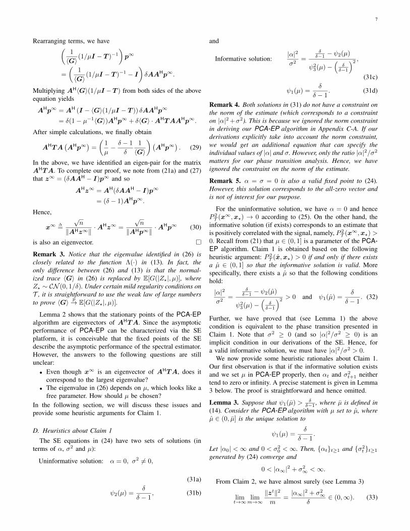
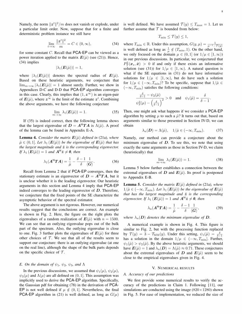
The above argument is not rigorous. However, our numericalresults suggest that the conclusions are correct. An exampleis shown in Fig. 2. Here, the figure on the right plots theeigenvalues of a random realization of E(µ) with n = 1500.We can see that an outlying eigenvalue pops out of the bulkpart of the spectrum. Also, the outlying eigenvalue is closeto one. Fig. 3 further plots the eigenvalues of E(µ) for threeother choices of T . We see that all of the results seem tosupport our conjecture: there is an outlying eigenvalue (at oneon the real line), although the shape of the bulk parts dependson the specific choice of T .

E. On the domain of ψ1, ψ2, ψ3, and Λ

In the previous discussions, we assumed that ψ1(µ), ψ2(µ),ψ3(µ) and Λ(µ) are all defined on (0, 1]. This assumption wasimplicitly used to derive the PCA-EP algorithm. Specifically,the Gaussian pdf for obtaining (78) in the derivation of PCA-EP is not well defined if µ /∈ (0, 1]. Nevertheless, the finalPCA-EP algorithm in (21) is well defined, as long as G(µ)

is well defined. We have assumed T (y) ≤ Tmax = 1. Let usfurther assume that T is bounded from below:

Tmin ≤ T (y) ≤ 1,

where Tmin ∈ R. Under this assumption, G(y, µ) = 1µ−1−T (y)

is well defined as long as 1µ /∈ (Tmin, 1). On the other hand,

we only focused on the domain µ ∈ (0, 1] (or 1/µ ∈ [1,∞))in our previous discussions. In particular, we conjectured thatP 2T (x?, x) > 0 if and only if there exists an informative

solution (see (31)) for 1/µ ∈ [1,∞). A natural question iswhat if the SE equations in (31) do not have informativesolutions for 1/µ ∈ [1,∞), but do have such a solutionfor 1/µ ∈ (−∞, Tmin)? To be specific, suppose that 1/µ ∈(−∞, Tmin) satisfies the following conditions:

δδ−1 − ψ2(µ)

ψ23(µ)−

(δδ−1

)2 > 0 and ψ1(µ) =δ

δ − 1.

Then, one might ask what happens if we consider a PCA-EPalgorithm by setting µ to such a µ? It turns out that, based onarguments similar to those presented in Section IV-D, we canobtain

λn(D) = Λ(µ), 1/µ ∈ (−∞, Tmin). (37)

Namely, our method can provide a conjecture about theminimum eigenvalue of D. To see this, we note that usingexactly the same arguments as those in Section IV-D, we claim(heuristically) that

limm→∞

λ1(E(µ)) = 1. (38)

Lemma 5 below further establishes a connection between theextremal eigenvalues of D and E(µ). Its proof is postponedto Appendix E-B.

Lemma 5. Consider the matrix E(µ) defined in (21a), where1/µ ∈ (−∞, Tmin). Let λ1 (E(µ)) be the eigenvalue of E(µ)that has the largest magnitude and z is the correspondingeigenvector. If λ1 (E(µ)) = 1 and AHz 6= 0, then

λn(AHTA) =1

µ− δ − 1

δ

1

〈G〉, (39)

where λn(D) denotes the minimum eigenvalue of D.

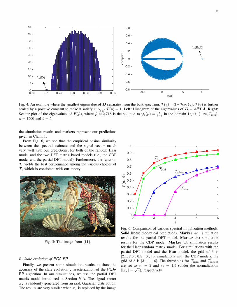
A numerical example is shown in Fig. 4. This figure issimilar to Fig. 2, but with the processing function replacedby T (y) = 3 − TMM(y). Under this setting, ψ1(µ) = δ

δ−1has a solution in the domain 1/µ ∈ (−∞, Tmin]. Further,ψ1(µ) > ψ2(µ). By the above heuristic arguments, we shouldhave E(µ) = 1 and λn(D) = Λ(µ) ≈ 0.71. These conjecturesabout the extremal eigenvalues of D and E(µ) seem to beclose to the empirical eigenvalues given in Fig. 4.

V. NUMERICAL RESULTS

A. Accuracy of our predictions

We first provide some numerical results to verify the ac-curacy of the predictions in Claim 1. Following [11], oursimulations are conducted using the image (820×1280) shownin Fig. 5. For ease of implementation, we reduced the size of

9

-0.5 -0.4 -0.3 -0.2 -0.1 0 0.1 0.2 0.30

5

10

15

20

25

30

35

40

45

61(D)

real-0.5 0 0.5 1

complex

-0.8

-0.6

-0.4

-0.2

0

0.2

0.4

0.6

0.8

61(E(7))

Fig. 2: Left: Histogram of the eigenvalues of D = AHTA. Right: Scatter plot of the eigenvalues of E(µ). µ is set to theunique solution to ψ1(µ) = δ

δ−1 . T = TMM. δ = 5. n = 1500. The signal x? is randomly generated from an i.i.d. zeroGaussian distribution.

real-0.5 0 0.5 1

complex

-0.8

-0.6

-0.4

-0.2

0

0.2

0.4

0.6

0.8

outlier

real-0.5 0 0.5 1

complex

-0.8

-0.6

-0.4

-0.2

0

0.2

0.4

0.6

0.8

outlier

real-0.5 0 0.5 1

complex

-0.8

-0.6

-0.4

-0.2

0

0.2

0.4

0.6

0.8

outlier

Fig. 3: Scatter plot of the eigenvalues of D2(µ1) in the complex plane. x? are sampled from an i.i.d. Gaussian distribution.n = 700, δ = 5. Left: T?, Middle: TMM, Right: Tsubset with c2 = 1.5.

the original image by a factor of 20 (for each dimension).The length of the final signal vector is 2624. We will comparethe performances of the spectral method under the followingmodels of A:• Random Haar model: A is a subsampled Haar matrix;• Coded diffraction patterns (CDP):

A =

FP1

FP2

. . .FPL

,where F is a two-dimensional DFT matrix and Pl =diag{ejθl,1 , . . . , ejθl,n} consists of i.i.d. uniformly ran-dom phases;

• Partial DFT model:

A = FSP ,

where, with slight abuse of notations, F ∈ Cm×m isnow a unitary DFT matrix, and S ∈ Rm×n is a random

selection matrix (which consists of randomly selectedcolumns of the identity matrix), and finally P is adiagonal matrix comprised of i.i.d. random phases.

Fig. 6 plots the cosine similarity of the spectral methodwith various choices of T . Here, the leading eigenvectoris computed using a power method. In our simulations, weapproximate T? by the function 1 −

(δy2 + 0.01

)−1. For

TMM and T?, the data matrix AHTA can have negativeeigenvalues. To compute the largest eigenvector, we run thepower method on the modified data matrix AHTA + εI fora large enough ε. In our simulations, we set ε to 10 forTMM and ε to 50 for T?. The maximum number of poweriterations is set to 10000. Finally, following [11], we measurethe images from the three RGB color-bands using independentrealizations of A. For each of the three measurement vectors,we compute the spectral estimator x and measure the cosinesimilarity PT (x?, x) and then average the cosine similarityover the three color-bands. Finally, we further average thecosine similarity over 5 independent runs. Here, the lines show

10

0.65 0.7 0.75 0.8 0.85 0.9 0.950

5

10

15

20

25

30

35

40

45

6n(D)

real-0.5 0 0.5 1

complex

-0.8

-0.6

-0.4

-0.2

0

0.2

0.4

0.6

0.8

61(E(7))

Fig. 4: An example where the smallest eigenvalue of D separates from the bulk spectrum. T (y) = 3−TMM(y). T (y) is furtherscaled by a positive constant to make it satisfy supy≥0 T (y) = 1. Left: Histogram of the eigenvalues of D = AHTA. Right:Scatter plot of the eigenvalues of E(µ), where µ ≈ 2.718 is the solution to ψ1(µ) = δ

δ−1 in the domain 1/µ ∈ (−∞, Tmin].n = 1500 and δ = 5.

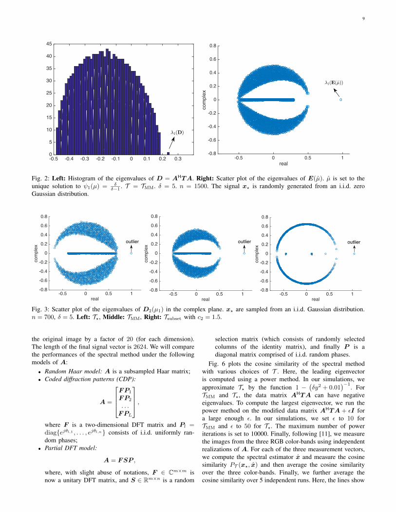
the simulation results and markers represent our predictionsgiven in Claim 1.

From Fig. 6, we see that the empirical cosine similaritybetween the spectral estimate and the signal vector matchvery well with our predictions, for both of the random Haarmodel and the two DFT matrix based models (i.e., the CDPmodel and the partial DFT model). Furthermore, the functionT? yields the best performance among the various choices ofT , which is consistent with our theory.

Fig. 5: The image from [11].

B. State evolution of PCA-EPFinally, we present some simulation results to show the

accuracy of the state evolution characterization of the PCA-EP algorithm. In our simulations, we use the partial DFTmatrix model introduced in Section V-A. The signal vectorx? is randomly generated from an i.i.d. Gaussian distribution.The results are very similar when x? is replaced by the image

/

2 3 4 5 6

P(x

?;x

)

0

0.1

0.2

0.3

0.4

0.5

0.6

0.7

0.8

0.9

1

Tsubset

Ttrim

TMM

T?

Fig. 6: Comparison of various spectral initialization methods.Solid lines: theoretical predictions. Marker +: simulationresults for the partial DFT model. Marker 4: simulationresults for the CDP model. Marker �: simulation resultsfor the Haar random matrix model. For simulations with thepartial DFT model and the Haar model, the grid of δ is[2.1, 2.5 : 0.5 : 6]; for simulations with the CDP models, thegrid of δ is [3 : 1 : 6]. The thresholds for Ttrim and Tsubset

are set to c1 = 2 and c2 = 1.5 (under the normalization‖x?‖ =

√n), respectively.

11

shown in Fig. 5. We consider an PCA-EP algorithm withµ = µ where µ is the solution to ψ1(µ) = δ

δ−1 .

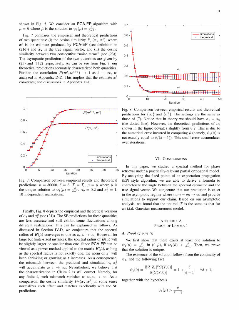
Fig. 7 compares the empirical and theoretical predictionsof two quantities: (i) the cosine similarity PT (x?,x

t), wherext is the estimate produced by PCA-EP (see definition in(21d)) and x? is the true signal vector, and (ii) the cosinesimilarity between two consecutive “noise terms” (see (23)).The asymptotic prediction of the two quantities are given by(25) and (112) respectively. As can be see from Fig. 7, ourtheoretical predictions accurately characterized both quantities.Further, the correlation P (wt,wt+1) → 1 as t → ∞, asanalyzed in Appendix D-D. This implies that the estimate xt

converges; see discussions in Appendix D-C.

iteration0 5 10 15 20 25 30 35

0

0.2

0.4

0.6

0.8

1

simulationstheoretical

P (wt!1;wt)

P (x?;xt)

Fig. 7: Comparison between empirical results and theoreticalpredictions. n = 30000. δ = 3. T = T?. µ = µ where µ isthe unique solution to ψ1(µ) = δ

δ−1 . α0 = 0.2 and σ20 = 1.

10 independent realizations.

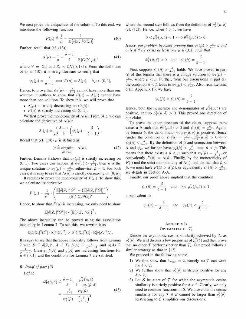
Finally, Fig. 8 depicts the empirical and theoretical versionsof αt and σ2

t (see (24)). The SE predictions for these quantitiesare less accurate and still exhibit some fluctuations amongdifferent realizations. This can be explained as follows. Asdiscussed in Section IV-D, we conjecture that the spectralradius of E(µ) converges to one as m,n→∞. However, forlarge but finite-sized instances, the spectral radius of E(µ) willbe slightly larger or smaller than one. Since PCA-EP can beviewed as a power method applied to the matrix E(µ), as longas the spectral radius is not exactly one, the norm of zt willkeep shrinking or growing as t increases. As a consequence,the mismatch between the predicted and simulated αt, σ

2t

will accumulate as t → ∞. Nevertheless, we believe thatthe characterization in Claim 2 is still correct. Namely, forany finite t, such mismatch vanishes as m,n → ∞. As acomparison, the cosine similarity PT (x?,x

t) in some sensenormalizes such effect and matches excellently with the SEpredictions.

iteration0 10 20 30 40 500

0.1

0.2

0.3

0.4

0.5

0.6

0.7

simulationstheoretical

,

<2

Fig. 8: Comparison between empirical results and theoreticalpredictions for {αt} and {σ2

t }. The settings are the same asthose of (7). Notice that in theory we should have αt = α0

(the dotted line). However, the theoretical predictions of αtshown in the figure deviates slightly from 0.2. This is due tothe numerical error incurred in computing µ (namely, ψ1(µ) isnot exactly equal to δ/(δ − 1)). This small error accumulatesover iterations.

VI. CONCLUSIONS

In this paper, we studied a spectral method for phaseretrieval under a practically-relevant partial orthogonal model.By analyzing the fixed points of an expectation propagation(EP) style algorithm, we are able to derive a formula tocharacterize the angle between the spectral estimator and thetrue signal vector. We conjecture that our prediction is exactin the asymptotic regime where n,m = δn→∞ and providesimulations to support our claim. Based on our asymptoticanalysis, we found that the optimal T is the same as that foran i.i.d. Gaussian measurement model.

APPENDIX APROOF OF LEMMA 1

A. Proof of part (i)

We first show that there exists at least one solution toψ1(µ) = δ

δ−1 in (0, µ), if ψ1(µ) > δδ−1 . Then, we prove

that the solution is unique.The existence of the solution follows from the continuity of

ψ1, and the following fact

ψ1(0) =E[δ|Z?|2G(Y, 0)]

E[G(Y, 0)]= 1 <

δ

δ − 1, ∀δ > 1,

together with the hypothesis

ψ1(µ) >δ

δ − 1.

12

We next prove the uniqueness of the solution. To this end, weintroduce the following function

F (µ)∆=

1

µ− 1

E [δ|Z?|2G(µ)]. (40)

Further, recall that (cf. (13))

Λ(µ) =1

µ− δ − 1

δ· 1

E [G(Y, µ)], (41)

where Y = |Z?| and Z? ∼ CN (0, 1/δ). From the definitionof ψ1 in (10), it is straightforward to verify that

ψ1(µ) =δ

δ − 1⇐⇒ F (µ) = Λ(µ), ∀µ ∈ (0, 1],

Hence, to prove that ψ1(µ) = δδ−1 cannot have more than one

solution, it suffices to show that F (µ) = Λ(µ) cannot havemore than one solution. To show this, we will prove that• Λ(µ) is strictly decreasing on (0, µ);• F (µ) is strictly increasing on (0, 1).We first prove the monotonicity of Λ(µ). From (41), we can

calculate the derivative of Λ(µ):

Λ′(µ) =1

µ2

δ − 1

δ

(ψ2(µ)− δ

δ − 1

).

Recall that (cf. (14)) µ is defined as

µ∆= argmin

µ∈(0,1]

Λ(µ). (42)

Further, Lemma 8 shows that ψ2(µ) is strictly increasing on(0, 1). Two cases can happen: if ψ2(1) > δ

δ−1 , then µ is theunique solution to ψ2(µ) = δ

δ−1 ; otherwise, µ = 1. For bothcases, it is easy to see that Λ(µ) is strictly decreasing on (0, µ).

It remains to prove the monotonicity of F (µ). To show this,we calculate its derivative:

F ′(µ) =1

µ2·

(E[δ|Z?|2G2]−

(E[δ|Z?|2G]

)2(E[δ|Z?|2G])

2

).

Hence, to show that F (µ) is increasing, we only need to show

E[δ|Z?|2G2] >(E[δ|Z?|2G]

)2.

The above inequality can be proved using the associationinequality in Lemma 7. To see this, we rewrite it as

E[δ|Z?|2G2] · E[δ|Z?|2] > E[δ|Z?|2G] · E[δ|Z?|2G].

It is easy to see that the above inequality follows from Lemma7 with B

∆= δ|Z?|2, A ∆

= T , f(A)∆= 1

µ−1−A , and g(A)∆=

1µ−1−A . Clearly, f(A) and g(A) are increasing functions forµ ∈ (0, 1], and the conditions for Lemma 7 are satisfied.

B. Proof of part (ii)

Define

θ2T (µ, δ)

∆=δ − 1

δ· ρ2

T (µ, δ)

1− ρ2T (µ, δ)

=δδ−1 − ψ2(µ)

ψ23(µ)−

(δδ−1

)2

(43)

where the second step follows from the definition of ρ2T (µ, δ)

(cf. (12)). Hence, when δ > 1, we have

0 < ρ2T (µ, δ) < 1⇐⇒ θ2

T (µ, δ) > 0.

Hence, our problem becomes proving that ψ1(µ) > δδ−1 if and

only if there exists at least one µ ∈ (0, 1] such that

θ2T (µ, δ) > 0 and ψ1(µ) =

δ

δ − 1.

First, suppose ψ1(µ) > δδ−1 holds. We have proved in part

(i) of this lemma that there is a unique solution to ψ1(µ) =δδ−1 , where µ < µ. Further, from our discussions in part (i),the condition µ < µ leads to ψ2(µ) < δ

δ−1 . Also, from Lemma6 (in Appendix F), we have

ψ3(µ) > ψ1(µ) =δ

δ − 1.

Hence, both the numerator and denominator of ρ2T (µ, δ) are

positive, and so ρ2T (µ, δ) > 0. This proved one direction of

our claim.To prove the other direction of the claim, suppose there

exists a µ such that θ2T (µ, δ) > 0 and ψ1(µ) = δ

δ−1 . Again,by lemma 6, the denominator of ρT (µ, δ) is positive. Hence(under the condition of ψ1(µ) = δ

δ−1 ), ρ2T (µ, δ) > 0 ⇐⇒

ψ2(µ) < δδ−1 . By the definition of µ and connection between

Λ and ψ2, we further have ψ2(µ) < δδ−1 ⇐⇒ µ < µ. This

means that there exists a µ < µ such that ψ1(µ) = δδ−1 , or

equivalently F (µ) = Λ(µ). Finally, by the monotonicity ofF (·) and the strict monotonicity of Λ(·), and the fact that µ <µ, we must have F (µ) > Λ(µ), or equivalently ψ1(µ) > δ

δ−1 ;see details in Section A-A.

Finally, our proof above implied that the condition

ψ1(µ) =δ

δ − 1and 0 < ρ2

T (µ, δ) < 1,

is equivalent to

ψ1(µ) =δ

δ − 1and ψ2(µ) <

δ

δ − 1.

APPENDIX BOPTIMALITY OF T?

Denote the asymptotic cosine similarity achieved by T? asρ2?(δ). We will discuss a few properties of ρ2

?(δ) and then provethat no other T performs better than T?. Our proof follows asimilar strategy as that in [12].

We proceed in the following steps:1) We first show that δweak = 2, namely no T can work

for δ < 2;2) We further show that ρ2

?(δ) is strictly positive for anyδ > 2;

3) Let S be a set of T for which the asymptotic cosinesimilarity is strictly positive for δ > 2. Clearly, we onlyneed to consider functions in S. We prove that the cosinesimilarity for any T ∈ S cannot be larger than ρ2

?(δ).Restricting to S simplifies our discussions.

13

A. Weak threshold

We first prove that δT is lower bounded by 2. Namely, ifδ < 2, then ρ2

T (δ) = 0 for any T . According to Claim 1, ifρ2T (δ) > 0, we must have ψ1(µ) ≥ δ

δ−1 . Further, Lemma 1shows that there is a unique solution to the following equation(denoted as µ)

ψ1(µ) =δ

δ − 1, µ ∈ (0, µ].

In Section A-A we have proved that

ψ2(µ) <δ

δ − 1⇐⇒ µ ∈ (0, µ].

Hence,ψ1(µ) > ψ2(µ).

From the definitions in (10) and noting G(y, µ) > 0 for anyµ ∈ (0, 1) and y ≥ 0, we can rewrite the condition ψ1(µ) >ψ2(µ) as

E[G2

1

]< E [G1] · E[δ|Z?|2G1], (44)

where we denoted G1∆= G(|Z?|, µ). Further, applying the

Cauchy-Schwarz inequality yields

(E[δ|Z?|2G1])2 ≤ E[δ2|Z?|4] · E[G21]

= 2 · E[G21],

(45)

where the second step (i.e., E[δ2|Z?|4] = 2) follows fromthe definition Z? ∼ CN (0, 1/δ) and direct calculations of thefourth order moment of |Z?|. Combining (44) and (45) yields

(E[δ|Z?|2G1])2 ≤ 2E [G1] · E[δ|Z?|2G1],

which further leads to

E[δ|Z?|2G1]

E [G1]≤ 2. (46)

On the other hand, the condition ψ1(µ) = δδ−1 gives us

E[δ|Z?|2G1]

E [G1]=

δ

δ − 1. (47)

Combining (46) and (47) leads to δδ−1 ≤ 2, and so δ ≥ 2.

This completes the proof.

We now prove that δ = 2 can be achieved by T?. When δ >2, we have δ

δ−1 ∈ (1, 2). Since T? is an increasing function, byLemma 8, both ψ1(µ) and ψ2(µ) are increasing functions onµ ∈ (0, 1). Further, it is straightforward to show that ψ1(0) =ψ2(0) = 1 and ψ1(1) = ψ2(1) = 2. Further, Lemma 9 (inAppendix F) shows that for T = T?

ψ2(µ) < ψ1(µ), ∀µ ∈ (0, 1).

The above facts imply that when δ > 2 we have

ψ1(µ) >δ

δ − 1,

where µ is the unique solution to

ψ2(µ) =δ

δ − 1.

Then, using Lemma 1 we proved ρ2?(δ) > 0 for δ > 2.

B. Properties of ρ2?(δ)

Since δweak = 2, we will focus on the regime δ > 2 in therest of this appendix.

For notational brevity, we will put a subscript ? to a variable(e.g., µ?) to emphasize that it is achieved by T = T?. Further,for brevity, we use the shorthand G? for G(|Z?|, µ). Letρ2?(δ) be the function value of achieved by T?. Further, for

convenience, we also define (see (43))

θ2?(δ)

∆=δ − 1

δ· ρ2

?(δ)

1− ρ2?(δ)

=

δδ−1 −

E[G2?]

E2[G?]

E[δ|Z?|2G2?]

E2[G?] −(

δδ−1

)2 ,(48)

where the last equality is from the definition in (12). We nextshow that P 2

? (δ) can be expressed compactly as

θ2?(δ) =

1

µ?− 1, (49)

where µ? is the unique solution to ψ1(µ) = δδ−1 in (0, 1).

Then, from (48), it is straightforward to obtain

ρ2?(δ) =

1− µ?1− 1

δ µ?.

For T? = 1− 1δ|Z?|2 , the function G?(|Z?|, µ?) (denoted as

G? hereafter) is given by

G?(|Z?|, µ?) =1

µ−1? − T?(|Z?|)

=µ?δ|Z?|2

(1− µ?)δ|Z?|2 + µ?,

(50)where µ? ∈ (0, 1] is the unique solution to

ψ1(µ?) =E[δ|Z?|2G?]

E[G?]=

δ

δ − 1. (51)

The existence and uniqueness of µ? (for δ > 2) is guaranteedby the monotonicity of ψ1 under T? (see Lemma 8). Ourfirst observation is that G? in (50) satisfies the followingrelationship:

µ?δ|Z?|2 − (1− µ?)δ|Z?|2G? = µ?G?. (52)

Further, multiplying both sides of (52) by G? yields

µ?δ|Z?|2G? − (1− µ?)δ|Z?|2G2? = µ?G

2?. (53)

Taking expectations over (52) and (53), and notingE[δ|Z?|2] = 1, we obtain

µ? − (1− µ?)E[δ|Z?|2G?

]= µ?E[G?],

(54a)

µ? · E[δ|Z?|2G?

]− (1− µ?)E

[δ|Z?|2G2

?

]= µ?E

[G2?

].

(54b)

Substituting (54b) into (48), and after some calculations, wehave

θ2?(δ) =

1− µ?µ?

·E[δ|Z?|2G2

?]E2[G?] − δ

δ−1 ·µ?

1−µ? ·(

1E[G?] − 1

)E[δ|Z?|2G2

?]E2[G?] −

(δδ−1

)2 ,

(55)

14

where we have used the identity ψ1(µ?) =E[δ|Z?|2G?]/E[G?] = δ/(δ − 1). From (55), to proveθ2?(δ) = µ−1

? − 1, we only need to prove

µ?1− µ?

·(

1

E[G?]− 1

)=

δ

δ − 1, (56)

which can be verified by combining (51) and (54a).Before leaving this section, we prove the monotonicity

argument stated in Theorem 1. From (49), to prove that ρ2?(δ)

(or equivalently θ2?(δ)) is an increasing function of δ, it suffices

to prove that µ?(δ) is a decreasing function of δ. This is adirect consequence of the following facts: (1) µ?(δ) is theunique solution to ψ1(µ) = δ

δ−1 in (0, 1), and (2) ψ1(µ) isan increasing function of µ. The latter follows from Lemma8 (T?(y) = 1− 1

δy2 is an increasing function).

C. Optimality of G?In the previous section, we have shown that the weak

threshold is δweak = 2. Consider a fixed δ (where δ > 2)and our goal is to show that ρ2

T (δ) ≤ ρ2?(δ) for any T .

We have proved ρ2?(δ) > 0 (the asymptotic cosine similar-

ity) for δ > 2. Hence, we only need to consider T satisfyingρ2T (δ) > 0 (in which case we must have ψ1(µ) > δ

δ−1 ),since otherwise T is already worse than T?. In Lemma 1,we showed that the phase transition condition ψ1(µ) > δ

δ−1can be equivalently reformulated as

∃µ ∈ (0, 1], 0 < ρ2T (µ, δ) < 1 and ψ1(µ) =

δ

δ − 1.

Also, from (43) we see that

0 < ρ2T (µ, δ) < 1⇐⇒ θ2

T (µ, δ) > 0.

From the above discussions, the problem of optimally design-ing T can be formulated as

supT , µ∈(0,1)

θ2T (δ, µ)

s.t. θ2T (δ, µ) > 0,

ψ1(µ) =δ

δ − 1.

(57)

In the above formulation, µ ∈ (0, µ) is treated as a variablethat can be optimized. In fact, for a given T , there cannotexist more than one µ ∈ (0, 1) such that ψ1(µ) = δ

δ−1 andθ2T (δ, µ) > 0 hold simultaneously (from Lemma 1). There

can no such µ, though. In such cases, it is understood thatθ2T (δ, µ) = 0.

Substituting in (10) and after straightforward manipulations,we can rewrite (57) as

supG(·)>0

δδ−1 −

E[G2]E2[G]

E[δ|Z?|2G2]E2[G] −

(δδ−1

)2 > 0

s.t.E[δ|Z?|2G]

E[G]=

δ

δ − 1,

(58)

where G(y, µ) is

G(y, µ) =1

µ−1 − T (y). (59)

Note that G(y, µ) ≥ 0 for µ ∈ (0, 1].At this point, we notice that the function to be optimized has

been changed to the nonnegative function G(·) (with µ beinga parameter). Hence, the optimal G(·) is clearly not unique.In the following, we will show that the optimal value of theobjective function cannot be larger than that ρ?(δ).

Consider G(·) be an arbitrary feasible function (satisfyingE[G] = 1), and let θ2(δ) (or simply θ2) be the correspondingfunction value of the objective in (58). We now prove thatθ(δ) ≤ θ?(δ) for any δ > 2. First, note that scaling thefunction G(·) by a positive constant does not change theobjective function and the constraint of the problem. Hence,without loss of generality and for simplicity of discussions,we assume

E[G] = 1.

Since θ2 is the objective function value achieved by G, bysubstituting the definition of G into (58), we have

δδ−1 − E[G2]

E[δ|Z?|2G2]−(

δδ−1

)2 = θ2. (60)

Some straightforward manipulations give us

E[(θ2δ|Z?|2 + 1)G2

]= θ2

(δ

δ − 1

)2

+δ

δ − 1. (61)

We assume θ2 > 0, since otherwise it already means thatG is worse than G? (note that θ2

? = µ−1? − 1 is strictly

positive). Hence, θ2δ|Z?|2 + 1 > 0, and we can lower boundE[(θ2δ|Z?|2 + 1)G2

]by

E[(θ2δ|Z?|2 + 1)G2

]≥

(E[δ|Z?|2G]

)2

E

[(δ|Z?|2√θ2δ|Z?|2+1

)2]

=

(δδ−1

)2

E[

δ2|Z?|4θ2δ|Z?|2+1

] ,(62)

where the first line follows from the Cauchy-Swarchz inequal-ity E[X2] ≥ E2[XY ]/E[Y 2], and the second equality is dueto the constraint E[|Z?|2G] = δ

δ−1 . Combining (61) and (62)yields

E[

δ2|Z?|4

θ2δ|Z?|2 + 1

]≥ 1

θ2 + δ−1δ

. (63)

Further, we note that

E[

δ2|Z?|4

θ2δ|Z?|2 + 1

]=

1

θ2

(E[δ|Z?|2]− E

[δ|Z?|2

θ2δ|Z?|2 + 1

])=

1

θ2

(1− E

[δ|Z?|2

θ2δ|Z?|2 + 1

]).

(64)

Then, substituting (64) into (63) gives us

E[

δ|Z?|2

θ2δ|Z?|2 + 1

]≤

δ−1δ

θ2 + δ−1δ

. (65)

15

Combining (64) and (65), we can finally get

E[

δ2|Z?|4θ2δ|Z?|2+1

]E[

δ|Z?|2θ2δ|Z?|2+1

] ≥ δ

δ − 1. (66)

It remains to prove

θ2 < θ2? =

1

µ?− 1. (67)

To this end, we note that substituting (50) into (51) yields

E[

δ2|Z?|4(µ−1? −1)δ|Z?|2+1

]E[

δ|Z?|2(µ−1? −1)δ|Z?|2+1

] =δ

δ − 1. (68)

From Lemma 8, the LHS of (66) (which is ψ1(1/(1 + θ2))under T?) is a strictly decreasing function of θ ∈ (0,∞).Hence, combining (66) and (68) proves (67).

APPENDIX CDERIVATIONS OF THE PCA-EP ALGORITHM

In this appendix, we provide detailed derivations for thePCA-EP algorithm, which is an instance of the algorithmproposed in [22], [34], [35], [39]. The PCA-EP algorithmis derived based on a variant of expectation propagation [15],referred to as scalar EP in [40]. The scalar EP approximationwas first mentioned in [16, pp. 2284] (under the name ofdiagonally-restricted approximation) and independently stud-ied in [17]1. An appealing property of scalar EP is thatits asymptotic dynamics could be characterized by a stateevolution (SE) procedure under certain conditions. Such SEcharacterization for scalar EP was first observed in [17]–[19]and later proved in [20], [21]. Notice that the SE actually holdsfor more general algorithms that might not be derived fromscalar EP [18], [20].

For simplicity of exposition, we will focus on the real-valued setting in this appendix. We then generalize the PCA-EP algorithm to the complex-valued case in a natural way(e.g., replacing matrix transpose to conjugate transpose, etc).

A. The overall idea

The leading eigenvector of D is a solution to the followingproblem:

min‖x‖=√n

−xTDx, (69)

where D is defined in (3), and the normalization ‖x‖ =√n

(instead of ‖x‖ = 1) is imposed for discussion convenience.By introducing a Lagrange multiplier λ, we further transformthe above problem into an unconstrained one:

minx∈Rn

−xTDx+ λ‖x‖2. (70)

To yield the principal eigenvector, λ should be set to

λ = λ1(D), (71)

1The algorithm in [17] is equivalent to scalar EP, but derived (heuristically)in a different way.

where λ1(D) denotes the maximum eigenvalue of D. Notethat the unconstrained formulation is not useful algorithmicallysince λ1(D) is not known a priori. Nevertheless, based onthe unconstrained reformulation, we will derive a set of self-consistent equations that can provide useful information aboutthe eigen-structure of D. Such formulation of the maximumeigenvector problem using a Lagrange multiplier has also beenadopted in [41].

Following [34], we introduce an auxiliary variable z = Axand reformulate (70) as

minx∈Rn,z∈Rm

−m∑a=1

|za|2 · T (ya)︸ ︷︷ ︸f2(z)

+λ‖x‖2︸ ︷︷ ︸f1(x)

+I(z = Ax). (72)

Our first step is to construct a joint pdf of x ∈ Rn and z ∈Rm:

`(x, z) =1

Zexp(−β · f2(z))︸ ︷︷ ︸

F2(z)

· exp(−β · f1(x))︸ ︷︷ ︸F1(x)

·I(z = Ax),

(73)where Z is a normalizing constant and β > 0 is a parameter(the inverse temperature). The factor graph corresponding tothe above pdf is shown in Fig. 9. Similar to [42], we derivePCA-EP based on the following steps:• Derive an EP algorithm, referred to as PCA-EP-β, for

the factor graph shown in Fig. 9;• Obtain PCA-EP as the zero-temperature limit (i.e., β →∞) of PCA-EP-β.

Intuitively, as β → ∞, the pdf `(x, z) concentrates aroundthe minimizer of (72). The PCA-EP algorithm is a low-costmessage passing algorithm that intends to find the minimizer.Similar procedure has also been used to derive an AMPalgorithm for solving an amplitude-loss based phase retrievalproblem [8, Appendix A].

We would like to point out that, for the PCA problem in(72), the resulting PCA-EP-β algorithm becomes invariant toβ (the effect of β cancels out). This is essentially due to theGaussianality of the factors F1(x) and F2(z) defined in (73),as will be seen from the derivations in the next subsections.Note that this is also the case for the AMP.S algorithm derivedin [8], which is an AMP algorithm for solving (72).

B. Derivations of PCA-EP-β

As shown in Fig. 9, the factor graph has three factor nodes,represented in the figure as F1(x), F2(z) and z = Axrespectively.

Before we proceed, we first point out that the message fromnode x to node z = Ax is equal to F1(x) = exp(−λ‖x‖2),and is invariant to its incoming message. This is essentiallydue to the fact that F1(x) is a Gaussian pdf with identicalvariances, as will be clear from the scalar EP update ruledetailed below. As a consequence, we only need to updatethe messages exchanged between node z = Ax and nodeF2(z); see Fig. 9. Also, due to the Gaussian approximationsadopted in EP algorithms, we only need to track the mean andvariances of these messages.

16

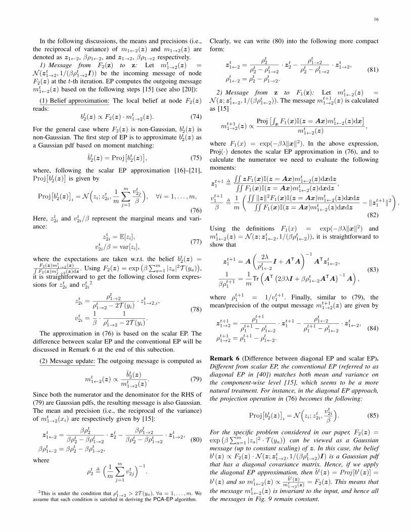
In the following discussions, the means and precisions (i.e.,the reciprocal of variance) of m1←2(z) and m1→2(z) aredenoted as z1←2, βρ1←2, and z1→2, βρ1→2 respectively.

1) Message from F2(z) to z: Let mt1→2(z) =

N (zt1→2, 1/(βρt1→2I)) be the incoming message of node

F2(z) at the t-th iteration. EP computes the outgoing messagemt

1←2(z) based on the following steps [15] (see also [20]):

(1) Belief approximation: The local belief at node F2(z)reads:

bt2(z) ∝ F2(z) ·mt1→2(z). (74)

For the general case where F2(z) is non-Gaussian, bt2(z) isnon-Gaussian. The first step of EP is to approximate bt2(z) asa Gaussian pdf based on moment matching:

bt2(z) = Proj[bt2(z)

], (75)

where, following the scalar EP approximation [16]–[21],Proj

[bt2(z)

]is given by

Proj[bt2(z)

]i

= N(zi; z

t2i,

1

m

m∑j=1

vt2jβ

), ∀i = 1, . . . ,m,

(76)Here, zt2i and vt2i/β represent the marginal means and vari-ance:

zt2i = E[zi],

vt2i/β = var[zi],(77)

where the expectations are taken w.r.t. the belief bt2(z) =F2(z)mt1→2(z)∫F2(z)mt1→2(z)dz

. Using F2(z) = exp(β∑ma=1 |za|2T (ya)

),

it is straightforward to get the following closed form expres-sions for zt2i and vt2i

2

zt2i =ρt1→2

ρt1→2 − 2T (yi)· zt1→2,i,

vt2i =1

β· 1

ρt1→2 − 2T (yi).

(78)

The approximation in (76) is based on the scalar EP. Thedifference between scalar EP and the conventional EP will bediscussed in Remark 6 at the end of this subection.

(2) Message update: The outgoing message is computed as

mt1←2(z) ∝ bt2(z)

mt1→2(z)

. (79)

Since both the numerator and the denominator for the RHS of(79) are Gaussian pdfs, the resulting message is also Gaussian.The mean and precision (i.e., the reciprocal of the variance)of mt

1→2(xi) are respectively given by [15]:

zt1←2 =βρt2

βρt2 − βρt1→2

· zt2 −βρt1→2

βρt2 − βρt1→2

· zt1→2,

βρt1←2 = βρt2 − βρt1→2,

(80)

where

ρt2∆=( 1

m

m∑j=1

vt2j

)−1

.

2This is under the condition that ρt1→2 > 2T (ya), ∀a = 1, . . . ,m. Weassume that such condition is satisfied in deriving the PCA-EP algorithm.

Clearly, we can write (80) into the following more compactform:

zt1←2 =ρt2

ρt2 − ρt1→2

· zt2 −ρt1→2

ρt2 − ρt1→2

· zt1→2,

ρt1←2 = ρt2 − ρt1→2.

(81)

2) Message from z to F1(z): Let mt1←2(z) =

N (z; zt1←2, 1/(βρt1←2)). The message mt+1

1→2(z) is calculatedas [15]

mt+11→2(z) ∝

Proj[∫xF1(x)I(z = Ax)mt

1←2(z)dx]

mt1←2(z)

,

where F1(x) = exp(−βλ‖x‖2). In the above expression,Proj(·) denotes the scalar EP approximation in (76), and tocalculate the numerator we need to evaluate the followingmoments:

zt+11

∆=

∫∫zF1(x)I(z = Ax)mt

1←2(z)dxdz∫∫F1(x)I(z = Ax)mt

1←2(z)dxdz,

vt+11

β

∆=

1

m

(∫∫‖z‖2F1(x)I(z = Ax)mt

1←2(z)dxdz∫∫F1(x)I(z = Ax)mt

1←2(z)dxdz− ‖zt+1

1 ‖2).

(82)

Using the definitions F1(x) = exp(−βλ‖x‖2) andmt

1←2(z) = N (z; zt1←2, 1/(βρt1←2)), it is straightforward to

show that

zt+11 = A

(2λ

ρt1←2

I +ATA

)−1

ATzt1←2,

1

βρt+11

=1

mTr(AT

(2βλI + βρt1←2A

TA)−1

A),

(83)

where ρt+11 = 1/vt+1

1 . Finally, similar to (79), themean/precision of the output message mt+1

1→2(z) are given by

zt+11→2 =

ρt+11

ρt+11 − ρt1←2

· zt+11 − ρt1←2

ρt+11 − ρt1←2

· zt1←2,

ρt+11→2 = ρt+1

1 − ρt1←2.

(84)

Remark 6 (Difference between diagonal EP and scalar EP).Different from scalar EP, the conventional EP (referred to asdiagonal EP in [40]) matches both mean and variance onthe component-wise level [15], which seems to be a morenatural treatment. For instance, in the diagonal EP approach,the projection operation in (76) becomes the following:

Proj[bt2(z)

]i

= N(zi; z

t2i,vt2iβ

). (85)

For the specific problem considered in our paper, F2(z) =exp

(β∑ma=1 |za|2 · T (ya)

)can be viewed as a Gaussian

message (up to constant scaling) of z. In this case, the beliefbt(z) ∝ F2(z) · N (z; zt1→2, 1/(βρ

t1→2)I) is a Gaussian pdf

that has a diagonal covariance matrix. Hence, if we applythe diagonal EP approximation, then bt(z) = Proj [bt(z)] =

bt(z) and so mt1←2(z) ∝ bt(z)

mt1→2(z)= F2(z). This means that

the message mt1←2(z) is invariant to the input, and hence all

the messages in Fig. 9 remain constant.

17

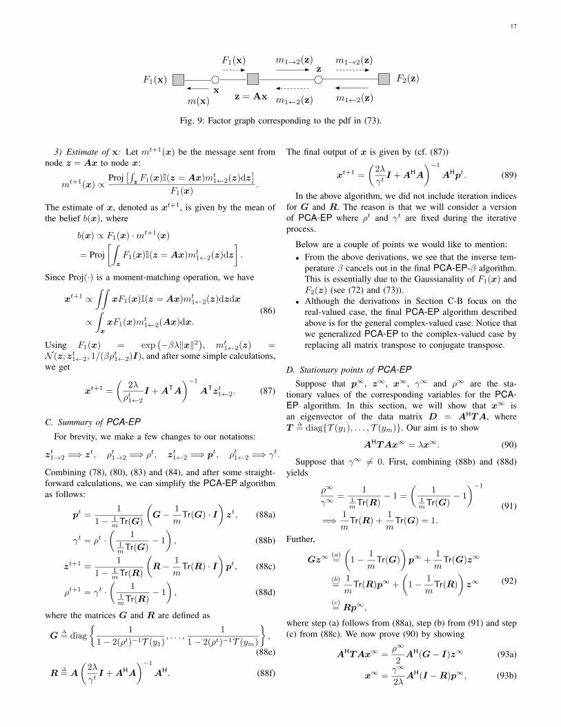
xz = Ax

m1→2(z)F1(x)

F2(z)

m1→2(z)

m1←2(z)

zF1(x)

m1←2(z)m(x)

Fig. 9: Factor graph corresponding to the pdf in (73).

3) Estimate of x: Let mt+1(x) be the message sent fromnode z = Ax to node x:

mt+1(x) ∝Proj

[∫zF1(x)I(z = Ax)mt

1←2(z)dz]

F1(x).

The estimate of x, denoted as xt+1, is given by the mean ofthe belief b(x), where

b(x) ∝ F1(x) ·mt+1(x)

= Proj[∫z

F1(x)I(z = Ax)mt1←2(z)dz

].

Since Proj(·) is a moment-matching operation, we have

xt+1 ∝∫∫

xF1(x)I(z = Ax)mt1←2(z)dzdx

∝∫x

xF1(x)mt1←2(Ax)dx.

(86)

Using F1(x) = exp(−βλ‖x‖2

), mt

1←2(z) =N (z; zt1←2, 1/(βρ

t1←2)I), and after some simple calculations,

we get

xt+1 =

(2λ

ρt1←2

I +ATA

)−1

ATzt1←2. (87)

C. Summary of PCA-EP

For brevity, we make a few changes to our notations:

zt1→2 =⇒ zt, ρt1→2 =⇒ ρt, zt1←2 =⇒ pt, ρt1←2 =⇒ γt.

Combining (78), (80), (83) and (84), and after some straight-forward calculations, we can simplify the PCA-EP algorithmas follows:

pt =1

1− 1mTr(G)

(G− 1

mTr(G) · I

)zt, (88a)

γt = ρt ·(

11mTr(G)

− 1

), (88b)

zt+1 =1

1− 1mTr(R)

(R− 1

mTr(R) · I

)pt, (88c)

ρt+1 = γt ·(

11mTr(R)

− 1

), (88d)

where the matrices G and R are defined as

G∆= diag

{1

1− 2(ρt)−1T (y1), . . . ,

1

1− 2(ρt)−1T (ym)

},

(88e)

R∆= A

(2λ

γtI +AHA

)−1

AH. (88f)

The final output of x is given by (cf. (87))

xt+1 =

(2λ

γtI +AHA

)−1

AHpt. (89)

In the above algorithm, we did not include iteration indicesfor G and R. The reason is that we will consider a versionof PCA-EP where ρt and γt are fixed during the iterativeprocess.

Below are a couple of points we would like to mention:• From the above derivations, we see that the inverse tem-

perature β cancels out in the final PCA-EP-β algorithm.This is essentially due to the Gaussianality of F1(x) andF2(z) (see (72) and (73)).

• Although the derivations in Section C-B focus on thereal-valued case, the final PCA-EP algorithm describedabove is for the general complex-valued case. Notice thatwe generalized PCA-EP to the complex-valued case byreplacing all matrix transpose to conjugate transpose.

D. Stationary points of PCA-EPSuppose that p∞, z∞, x∞, γ∞ and ρ∞ are the sta-

tionary values of the corresponding variables for the PCA-EP algorithm. In this section, we will show that x∞ isan eigenvector of the data matrix D = AHTA, whereT

∆= diag{T (y1), . . . , T (ym)}. Our aim is to show

AHTAx∞ = λx∞. (90)

Suppose that γ∞ 6= 0. First, combining (88b) and (88d)yields

ρ∞

γ∞=

11mTr(R)

− 1 =

(1

1mTr(G)

− 1

)−1

=⇒ 1

mTr(R) +

1

mTr(G) = 1.

(91)

Further,

Gz∞(a)=

(1− 1

mTr(G)

)p∞ +

1

mTr(G)z∞

(b)=

1

mTr(R)p∞ +

(1− 1

mTr(R)

)z∞

(c)= Rp∞,

(92)

where step (a) follows from (88a), step (b) from (91) and step(c) from (88c). We now prove (90) by showing

AHTAx∞ =ρ∞

2AH(G− I)z∞ (93a)

x∞ =γ∞

2λAH(I −R)p∞, (93b)

18

and

(G− I)z∞ =γ∞

ρ∞(I −R)p∞. (93c)

We next prove (93a). By using (89), we have

AHTAx∞ = AHTA

(2λ

γ∞I +AHA

)−1

AHp∞

(a)= AHTRp∞

(b)= AHTGz∞

(c)=ρ∞

2AH(G− I)z∞,

where (a) is from the definition of R in (88f), (b) is due to(92), and finally (c) is from the identity TG = ρ∞

2 (G − I)that can be verified from the definition of G in (88e).

We now prove (93b). From (88f), we have

AH(I −R)z∞ =

(AH −AHA

(2λ

γ∞I +AHA

)−1

AH

)z∞

=

(I −AHA

(2λ

γ∞I +AHA

)−1)AHz∞

=2λ

γ∞

(2λ

γ∞I +AHA

)−1

AHz∞

=2λ

γ∞x∞

where the last step is from the definition of x∞ in (89).Finally, we prove (93c). From (88a) and (88c), we have

(G− I)z∞ =

(1− 1

mTr(G)

)(p∞ − z∞) ,

(R− I)p∞ =

(1− 1

mTr(R)

)(z∞ − p∞) .

Then, (93c) follows from these identities together with (91).

E. PCA-EP with fixed tuning parameters

We consider a version of PCA-EP where ρt = ρ and γt =γ, ∀t, where ρ > 0 and γ ∈ R are understood as tuningparameters. We further assume that ρ and γ are chosen suchthat the following relationship holds (cf. 91):

1

mTr(G) +

1

mTr(R) = 1.

Under the above conditions, the PCA-EP algorithm in (88)can be written into the following compact form:

zt+1 =

(R

1mTr(R)

− I)(

G1mTr(G)

− I)zt, (94)

where G and R are defined in (88e) and (88f), respectively.Further, there are three tuning parameters involved, namely, λ,ρ and γ.

F. PCA-EP for partial orthogonal matrix

The PCA-EP algorithm simplifies considerably for partialorthogonal matrices satisfying AHA = I . To see this, notethat R in (88f) becomes (with γt = γ)

R =1

2λγ + 1

·AAH. (95)

Since1

mTr(AAH) =

n

m=

1

δ,

we haveR

1mTr(R)

= δAAH.

Then, using the above identity and noting the constraint1mTr(R) + 1

mTr(G) = 1 (cf. (91)), we could write (94) intothe following update:

zt+1 =(δAAH − I

)( G1mTr(G)

− I)zt, (96)

where

G∆= diag

{1

1− 2(ρ)−1T (y1), . . . ,

1

1− 2(ρ)−1T (ym)

}We will treat the parameter ρ as a tunable parameter for PCA-EP . Finally, we note that (96) is invariant to a scaling of G.We re-define G into the following form:

G = diag

{1

µ−1 − T (y1), . . . ,

1

µ−1 − T (ym)

},

where µ is a tunable parameter. This form of G is moreconvenient for certain parts of our discussions.

APPENDIX DHEURISTIC DERIVATIONS OF STATE EVOLUTION

The PCA-EP iteration is given by

zt+1 = (δAAH − I)

(G

〈G〉− I

)zt, (97a)

with the initial estimate distributed as

z0 d= α0z? + σ0w

0, (97b)

and w0 ∼ CN (0, 1/δI) is independent of z?. An appealingproperty of PCA-EP is that zt (for t ≥ 1) also satisfies theabove “signal plus white Gaussian noise” property:

ztd= αtz? + σ0w

t,

where wt is independent of z?. In the following sections, wewill present a heuristic way of deriving• The mapping (αt, σ

2t ) 7→ (αt+1, σ

2t+1);

• The correlation between the estimate xt+1 and and truesignal x?:

ρ(X?, Xt+1)

∆= limm→∞

〈x?,xt+1〉‖xt+1‖‖x?‖

;

• The correlation between two consecutive “noise” terms:

ρ(W t,W t+1)∆= limm→∞

〈wt,wt+1〉‖wt‖‖wt+1‖

.

19

A. Derivations of {αt} and {σt}

We now provide a heuristic derivation for the SE recursiongiven in (24). For convenience, we introduce an auxiliaryvariable:

pt∆=

(G

〈G〉− I

)zt︸ ︷︷ ︸

Hdf(zt,y;µ)

(98)

where 〈G〉 ∆= 1

mTr(G). Further, based on a heuristic concen-tration argument, we have

〈G〉 ≈ G = E [G] ,

where

G∆=

1

µ−1 − T (|Z?|)

and the expectation is taken over Z? ∼ CN (0, 1/δ). The intu-ition of PCA-EP is that, in each iteration, zt is approximatelydistributed as

ztd= αtz? + σtw

t, (99)

where wt ∼ CN (0, 1/δI) is independent of z?. Due to thisproperty, the distribution of zt is fully characterized by αtand σt. State evolution (SE) refers to the map (αt, σ

2t ) 7→

(αt+1, σ2t+1). It is possible to justify this property using the

conditioning lemma developed in [20], [21]. A rigorous proofis beyond the scope of this paper. Instead, we will only providea heuristic way of deriving the SE maps.

We first decompose pt into a vector parallel to z? and avector perpendicular to it:

pt =〈z?,pt〉‖z?‖2︸ ︷︷ ︸αpt

·z? +

(pt − 〈z?,p

t〉‖z?‖2

· z?)

︸ ︷︷ ︸ξ

, (100)

where

αpt ≈ δ · E[Z∗?Pt]

= δ · E[Z∗?

(G

G− 1

)Zt]

(a)= δ · E

[|Z?|2

(G

G− 1

)]· αt

(b)=(ψ1(µ)− 1

)· αt,

(101)

where step (a) is from our assumption Zt = αtZ?+W t whereW t is independent of Z? and step (b) is from the definitionof ψ1 (see (10)). Now, consider the update of zt+1 given in(94):

zt+1 = (δAAH − I)pt

= (δAAH − I) (αptz? + ξ)

= (δ − 1) · αpt · z? + (δAAH − I)ξ︸ ︷︷ ︸wt+1

,(102)

where in the last step we used AAHz? = AAHAx? =Ax? = z?. To derive the SE map, it remains to calculatethe (average) variance of the “effective noise” (δAAH− I)ξ:

1

mE‖(δAAH − I)ξ‖2

(a)=

tr(δAAH − I)2

m· E[|Ξ|2]

(b)= (δ − 1) · E[|Ξ|2]

(c)= (δ − 1) ·

(E[|Hdf |2

]− |αpt |

2 · E[|Z?|2])

(d)= (δ − 1) ·

(E[|Hdf |2

]− 1

δ· (ψ1(µ)− 1)

2 |αt|2)

(103)

where step (a) follows from the heuristic assumption that ξis “independent” of A3, step (b) is from AHA = I and thedefinition δ = m

n , step (c) is from the orthogonality betweenZ? and Ξ = Hdf − αptZ?, and step (d) from (101).

Next, we simplify the map (αt, σ2t ) 7→ σ2

t+1. Similar to step(c) of (103), we have

E[|Ξ|2] = E[|Hdf |2

]− |αpt |

2 · E[|Z?|2]

(a)= |αt|2 · E

[(G

G− 1

)2

|Z?|2]

+σ2t

δ· E

[(G

G− 1

)2]− 1

δ|αpt |

2

= |αt|2 ·

(E[|Z?|2G2

]G2

+1

δ−

2E[|Z?|2G

]G

)

+σ2t

δ

(E[G2]

G2− 1

)− 1

δ|αpt |

2

(b)= |αt|2

(ψ2

3(µ) + 1− 2ψ1(µ)

δ

)+σ2t

δ(ψ2(µ)− 1)

− |αt|2

δ·(ψ1(µ)− 1

)2=

1

δ·[|αt|2 ·

(ψ2

3(µ)− ψ21(µ)

)+ σ2

t ·(ψ2(µ)− 1

)],

(104)

where step (a) follows from the definition Zt = αtZ? + σtWwith W ∼ CN (0, 1/δ), and step (b) follows from the defini-tions in (10), and (c) from (10) and (101).

From (100), and (102)-(104), and recalling our definitionsof αt+1, σt+1 in (99), we have

αt+1 = (δ − 1) · (ψ1(µ)− 1) · αt, (105a)

σ2t+1 = (δ − 1)δ · E[|Ξ|2] (105b)

= (δ − 1) ·(|αt|2

(ψ2

3(µ)− ψ21(µ)

)+ σ2

t

(ψ2(µ)− 1

)).

Notice that the extra scaling δ in (105b) (compared with (103))is due to our assumption that E[|W |2] = 1/δ rather thanE[|W |2] = 1. In what follows, we will express the SE mapsin (105) using the functions ψ1, ψ2 and ψ3 defined in (10).

B. Derivations of ρ(X?, Xt+1)

From (102), we have

zt+1 = (δ − 1) · αpt · z? + (δAAH − I)ξ,

3We do not expect them to be truly independent. However, we expect theSE maps derived under this assumption to be correct.

20

where ξ is assumed to be independent of A. Recall that thefinal estimate xt+1 is defined as (cf. (21d))

xt+1 ∝ AHzt+1

= (δ − 1) · αpt ·AHAx? + (δ − 1)AHξ

= (δ − 1) · αpt︸ ︷︷ ︸αt+1

x? + (δ − 1)AHξ.

Intuitively, AHξ is a Gaussian noise term independent of x?,and composed of i.i.d. entries. Its average variance is given by

1

nE[|AHξ|2

]=

1

nTrE

[AHξξHA

]= E[|Ξ|2] · 1

nTrE

[AHA

]= E[|Ξ|2],

where the first two steps are from our heuristic assumptionsthat ξ is independent of A and consists of i.i.d. entries. Thecosine similarity is then given by

〈x?,xt+1〉‖xt+1‖‖x?‖

≈ αt+1√|αt+1|2 + (δ − 1)2E[|Ξ|2]

=αt+1√

|αt+1|2 + δ−1δ · σ

2t+1

,

where the last step is from (103) and (105b).

C. Derivations of ρ(W t,W t+1)

For notational convenience, we rewrite (99) as

ztd= αtz? + wt, (106)

where we defined wt ∆= σtw

t. In this section, we assumethat α0 ∈ R and so αt ∈ R for t ≥ 1; see (24a). Toanalyze the behavior of the PCA-EP algorithm, we needto understand the evolution of the correlation between twoconsecutive estimates, or equivalently the correlation betweentwo noise terms wt and wt+1:

ρ(wt,wt+1) = ρ(wt, wt+1)∆=〈wt, wt+1〉‖wt‖‖wt+1‖

. (107)

We assume that this empirical correlation term converges asm,n→∞, namely,

ρ(W t, W t+1)∆= limm→∞

ρ(wt, wt+1).

Suppose that ρ(wt, wt+1) → 1 as t → ∞, and the variablesαt and σ2

t converge to nonzero constants. Then, from (106), itis straightforward to show that zt converges under an appro-priate order, namely, limt→∞ limm→∞ 1

m‖zt − zt+1‖2 = 0.

This implies limt→∞ limn→∞ 1n‖x

t − xt+1‖ → 0 (wherext ∝ AHzt), since

‖AHzt −AHzt+1‖ ≤ ‖A‖ · ‖zt − zt+1‖ = ‖zt − zt+1‖.

Similarly, we can also show that 1n‖x

t − xt+s‖ → 0 for anys ≥ 1, under the above convergence order. This implies theconvergence of {xt}.

From Claim 2, as m,n→∞, almost surely we have

1

m‖wt‖‖wt+1‖ → σtσt+1

δ. (108)

Hence, to understand the evolution of ρ(wt, wt+1), it sufficesto understand the evolution of 1

m 〈wt, wt+1〉. We assume that

this empirical correlation term converges as m,n → ∞,namely,

1

m〈wt, wt+1〉 → E

[(W t)∗W t+1

],

where W t ∼ CN (0, σ2t /δ) and W t+1 ∼ CN (0, σ2

t+1/δ).To this end, we will derive a recursive formula for calculat-ing E

[(W t)∗W t+1

], namely, the map E

[(W t)∗W t+1

]7→

E[(W t+1)∗W t+2

].

First, given E[(W t)∗W t+1], we can calculate E[(P t)∗P t+1]as

E[(P t)∗P t+1](a)= E

[(G

G− 1

)2

(Zt)∗Zt+1

]

= E

[(G

G− 1

)2 (αtZ? + W t

)∗ (αt+1Z? + W t+1

)](b)= αtαt+1E

[(G

G− 1

)2

|Z?|2]

+ E

[(G

G− 1

)2]E[(W t)∗W t+1]

(c)=αtαt+1

δ

(ψ2

3(µ) + 1− 2ψ1(µ))

+ (ψ2(µ)− 1)E[(W t)∗W t+1],

(109)

where step (a) is from (98), step (b) is due to the independencebetween (W t, W t+1) and Z?, and step (c) follows from thedefinitions of ψ1, ψ2 and ψ3 in (10).

From (100), we have

P t = αtpZ? + Ξt,

where Ξt is orthogonal to Z? (i.e., E[(Z?)∗Ξ] = 0). Hence,

E[(Ξt)∗Ξt+1] = E[(P t)∗P t+1]−αptα

pt+1

δ. (110)

Finally, we establish the relationship between E[(Ξt)∗Ξt+1]and E[(W t+1)∗W t+2]. This step is similar to our derivationsof the SE map in (103). Note that

wt+1 = (δAAH − I)ξt.

Then,

E[(W t+1)∗W t+2] ≈ 1

m(wt+1)Hwt+2

=1

mTr((δAAH − I)ξt+1(ξt)H(δAAH − I)

)=

1

mTr((δAAH − I)2ξt+1(ξt)H

)(a)≈ 1

mTr((δAAH − I)2

)· 1

mTr(ξt+1(ξt)H)

≈ (δ − 1) · E[(Ξt)∗Ξt+1],(111)

where step (a) follows from a heuristic assumption that(ξt, ξt+1) are “independent of” (δAAH − I). Combining(109), (110) and (111) yields the following (see equation onthe top of next page).

Finally, we derive the initial condition for the above re-cursion (i.e., E[(W 0)∗W 1]). Recall that we assumed z0 =

21

E[(W t+1)∗W t+2] = (δ − 1) ·(αtαt+1

δ·(ψ2

3(µ) + 1− 2ψ1(µ))

+ (ψ2(µ)− 1) · E[(W t)∗W t+1]−αptα

pt+1

δ

)= (δ − 1) ·

(αtαt+1

δ·(ψ2

3(µ)− ψ21(µ)

)+ (ψ2(µ)− 1) · E[(W t)∗W t+1]

).

(112)

α0z?+ w0, where w0 ∼ CN (0, σ20/δI) is independent of z?.

Similar to the above derivations, w1 can be expressed as

w1 = (δAAH − I)ξ0.

Then,

E[(W 0)∗W 1] ≈ 1

m(w0)Hw1

=1

mTr((δAAH − I)ξ0(w0)H

)(a)≈ 1

mTr((δAAH − I)

)· 1

mTr(ξ0(w0)H

)= 0,

where step (a) is due to the heuristic assumption that (w0, ξ0)are “independent of” δAAH − I (similar to (111)).

D. Convergence of ρ(W t,W t+1)

Suppose that the phase transition condition in Claim 1 issatisfied. Specifically, ψ1(µ) > δ

δ−1 , where µ is defined in(14). Let µ ∈ (0, µ] be the unique solution to ψ1(µ) = δ

δ−1 .Consider an PCA-EP algorithm with µ = µ. Under thischoice, it is straightforward to show that

αt = α0, ∀t ≥ 1,

where {αt}t≥1 is generated according to (24a). Assume thatα0 6= 0. (We have assumed α0 ∈ R in the previous section.)The recursion in (112) becomes

E[(W t+1)∗W t+2] =(δ − 1)α2

0

δ·(ψ2

3(µ)− ψ21(µ)

)+ (δ − 1) (ψ2(µ)− 1) · E[(W t)∗W t+1].

From Lemma A, we have ψ2(µ) < δδ−1 , and so

(δ − 1) (ψ2(µ)− 1) < 1.

Further, Lemma 6 shows that ψ23(µ) − ψ2

1(µ) > 0. Hence,E[(W t+1)∗W t+2] converges:

limt→∞

E[(W t+1)∗W t+2] =α2

0

δ· ψ

23(µ)− ψ2

1(µ)δδ−1 − ψ2(µ)

=1

δ· limt→∞

σ2t ,

(113)where the second equality can be easily verified from (24b).Combining (107), (108), and (113) leads to

limt→∞

ρ(W t,W t+1) = limt→∞

ρ(W t, W t+1)

=limt→∞ E[(W t+1)∗W t+2]

σ2/δ= 1.

APPENDIX ECONNECTIONS BETWEEN THE EXTREME EIGENVALUES OF

D AND E(µ)

A. Proof of Lemma 4

Note that we assumed µ ∈ (0, 1] in Lemma 4. As mentionedin Remark 3, we could replace the average trace 〈G〉 in E(µ)by its asymptotic limit G = E[G(|Z?|, µ)], and consider thefollowing matrix instead:

E(µ) =(δAAH − I

)(GG− I

)= δAAH

(G

G− I

)−(G

G− I

),

where throughout this appendix we denote

G∆= (1/µI − T )−1.

We next prove that if the spectral radius of E(µ) is one, i.e.,

|λ1(E(µ))| = 1,

then

λ1(D) ≤ Λ(µ) =1

µ− δ − 1

δ· 1

E[G(|Z?|, µ)].

The characteristic polynomial of E(µ) is given by

f(t) = det(tI −E(µ))

= det

(tI +

(G

G− I

)− δAAH

(G

G− I

))= det

((t− 1)I +

G

G− δAAH

(G

G− I

) ).

(114)

Under the condition that |λ1(E(µ)| = 1, the characteristicpolynomial f(t) would have no root in t ∈ (1,∞):

f(t) 6= 0, ∀t > 1. (115)

(Here we focus on real-valued t, which will be enough forour purpose.) Note that the diagonal matrix (t − 1)I + G

Gis

invertible for t > 1 since G is a diagonal matrix with positiveentries:

Gi,i =1

1/µ− T (yi)> 0. (116)

Further, G = E[G(|Z?|, µ)] is also positive. Hence, f(t) in(114) can be rewritten as (117) (see the top of the next page),where step (a) is from the identity det(PQ) = det(P ) det(Q)and step (b) from det(I−PQ) = det(I−QP ). Recall from(115) that f(t) 6= 0 for t > 1. Hence,

g(t) 6= 0, t > 1. (118)

22

f(t) = det

((t− 1)I +

G

G− δAAH

(G

G− I

))(a)= det

((t− 1)I +

G

G

)· det

[I − δAAH

(G

G− I

)((t− 1)I +

G

G

)−1]

(b)= det

((t− 1)I +

G

G

)· det

[I − δAH

(G

G− I

)((t− 1)I +

G

G

)−1

A

]︸ ︷︷ ︸

g(t)

,

(117)

Define

B(t)∆= δAH

((t− 1)I +

G

G

)−1(G

G− I

)A, t > 1.

(119)The condition g(t) = det(I − B(t)) 6= 0 for t > 1 isequivalent to

λi(B(t)) 6= 1, ∀i = 1, . . . ,m, and t > 1,

where λi(B(t)) denotes the ith largest eigenvalue of B(t). Itis straightforward to see that the entries of B(t) converge tozero as t→∞:

limt→∞

B(t) = 0. (120)

Hence, all the eigenvalues of B(t) converge to zero as t→∞.At this point, we note that the eigenvalues of a matrix arecontinuous functions of it entries. (This observation has beenused in [11], but for a different purpose.) Hence, as t variesin [1,∞], λ1(B(t)) can take any value in [0, λ1(B(1))]. Inother words, for any C ∈ [0, λ1(B(1))], there exists somet? ∈ [1,∞] such that λ1(B(t?)) = C. Hence, (120) implies

λ1(B(t)) 6= 1, ∀t > 1. (121)

This means that the interval [0, λ1(B(1))) does not contain 1.Therefore, we must have

λ1(B(1)) 6 1. (122)

From (119) when t = 1, B(t) simplifies into

B(1) =

[δAH

((t− 1)I +

G

G

)−1(G

G− I

)A

]∣∣∣∣∣t=1

= δAH

(G

G

)−1(G

G− I

)A

= δAH[I − GG−1]A

= δ

(1− G

µ

)I + δGAHTA,

where the last step follows from the definition G = (1/µI −T )−1, and the assumption AHA = I . Hence, λ1(B(1)) 6 1(see (122)) readily leads to

λ1(AHTA) 61− (δ − δG/µ)

δG

=1

µ− δ − 1

δ· 1

G= Λ(µ),

where the last step is from (13). Also, we assumed 1 is aneigenvalue of E(µ). By Lemma 2, this implies that Λ(µ) isan eigenvalue of D. Summarizing, we have

λ1(AHTA) = Λ(µ).

B. Proof of Lemma 5

We only need to make a few minor changes to the proof inAppendix E-A. When 1/µ ∈ (−∞, Tmin), we have

G(y, µ) =1

µ−1 − T (y)< 0, ∀y ≥ 0,

1

µ∈ (−∞, Tmin).

Hence,

G = E[

1

1/µ− T (|Z?|)

]< 0,

1

µ∈ (−∞, Tmin).

(On the other hand, G(y, µ) > 0 when 1/µ ∈ [1,∞).) SinceG(y, µ) < 0 for arbitrary y ≥ 0, the diagonal matrix G/Ghas positive entries and is invertible. Following the proof inAppendix E-A, we still have

λ1(B(1)) ≤ 1, (123a)

whereB(1) = (δ − δG/µ) + δGAHTA. (123b)

Different from Appendix E-A, here we have G < 0, and from(123) and (123b) we have

λn(AHTA) ≥ 1

µ− δ − 1

δ· 1

G= Λ(µ).

Also, we assumed 1 is an eigenvalue of E(µ). By Lemma 2,this implies that Λ(µ) is an eigenvalue of D. Summarizing,we have

λn(AHTA) = Λ(µ).

APPENDIX FAUXILIARY LEMMAS

In this appendix, we collect some results regarding thefunctions ψ1, ψ2 and ψ3 defined in (10).

Lemma 6 (Auxiliary lemma). For any µ ∈ [0, 1], we have

ψ3(µ) ≥ ψ1(µ), (124)

Further, equality only holds at µ = 0.

23

Proof: From the definitions in (10), it’s equivalent toprove the following:

E[δ|Z?|2G2(Y, µ)

]≥(E[δ|Z?|2G(Y, µ)

])2.

This follows from the Cauchy-Schwarz inequality:

E[δ|Z?|2G(Y, µ)

]= E [δ|Z?|G(Y, µ) · |Z?|]≤√

E [δ|Z?|2G2(Y, µ)] · E [δ|Z?|2]

=√

E [δ|Z?|2G2(Y, µ)],

where the last equality is due to E[δ|Z?|2

]= 1.

Lemma 7 (Chebyshev’s association inequality [43]). Let fand g be nondecreasing real-valued functions. If A is a real-valued random variable and B is a nonnegative randomvariable, then

E[B] · E[Bf(A)g(A)] ≥ E[Bf(A)] · E[Bg(A)].

Lemma 8 (Monotonicity of ψ1 and ψ2). The function ψ2 in(10) is strictly increasing on (0, 1). Further, if T (y) is anincreasing function, then ψ1(µ) is strictly increasing on (0, 1).

Proof: Let Z? ∼ CN (0, 1/δ). For brevity, we denoteG(|Z?|, µ) as G. Further, the derivative G′(|Z?|, µ) (or simplyG′) is with respect to µ. From the definition of ψ2 in (10), itis straightforward to show that

ψ′2(µ) = 2 · E[GG′] · E[G]− E[G2] · E[G′]

(E[G])3

(a)=

2

µ2·E[G3] · E[G]− E

([G2]

)2(E[G])

3 ,

(125)

where step (a) follows from

G′(Y, µ) =1

(1− µT (Y ))2=G2

µ2.

Hence, to prove the monotonicity of ψ2, it remains to prove

E[G3] · E[G] > E([G2]

)2, ∀µ ∈ (0, 1),

which is a direct consequence of Lemma 7 (with A = B = G,f(A) = g(A) = A).

We next prove that ψ1 is also an increasing function underthe additional assumption that T (y) is an increasing functionof y. The derivative of ψ1 is given by (cf. 10):

ψ′1(µ) =E[δ|Z?|2G′

]· E [G]− E

[δ|Z?|2G

]· E [G′]

(E[G])2

(126a)

=1

µ2· E[δ|Z?|2G2] · E[G]− E[δ|Z?|2G] · E[G2]

(E[G])2

(126b)

Hence, we only need to prove

E[δ|Z?|2G2] · E[G] > E[δ|Z?|2G] · E[G2]

under the condition that T (y) is an increasing function. Again,this inequality follows from Lemma 7 by letting B = G,A = |Z?|, f(A) = A2 and g(A) = G(A,µ). Note that in thiscase G(|Z?|, µ) > 0 is an increasing function is |Z?| for any

µ ∈ (0, 1). Hence, both f(·) and g(·) are increasing functionsand the conditions in Lemma 7 are satisfied.

Lemma 9. When T (y) = T?(y)∆= 1− 1

δy2 , we have

ψ1(µ) > ψ2(µ), for µ ∈ (0, 1). (127)

Proof: From the definitions in (10), (127) is equivalent to

E[δ|Z?|2G(Y, µ)

]·E[G(Y, µ)] > E[G2(Y, µ)], for µ ∈ (0, 1),

(128)where Y = |Z?| and Z? ∼ CN (0, 1/δ). Since E[δ|Z?|2] = 1,we can write (128) as

E[δ|Z?|2G(Y, µ)

]· E[G(Y, µ)] > E[G2(Y, µ)] · E[δ|Z?|2].

(129)We will use Lemma 7 to prove (129). Specifically, we applyLemma 7 by specifying the random variables A and B, andthe functions f and g as follows:

A = |Z?|,B = G(Y, µ),

f(A) = δA2 · 1

G(A,µ),

g(A) = G(A,µ).

It is easy to show that B > 0 and g(·) is an increasing function;it only remains to prove that f(·) is an increasing function.From the definitions G(y, µ) = (1/µ− T (y))

−1 and T (y) =1− 1/(δy2), we have

f(A) = δA2 · 1

G(A,µ)

= δA2 ·(

1

µ− T (A)

)= δA2 ·

(1

µ−(

1− 1

δA2

))=

1− µµ

δA2 + 1,

which is an increasing function of A (which is defined on R+)when µ ∈ (0, 1). This completes our proof.

REFERENCES

[1] Y. Shechtman, Y. C. Eldar, O. Cohen, H. N. Chapman, J. Miao, andM. Segev, “Phase retrieval with application to optical imaging: Acontemporary overview,” IEEE Signal Process. Mag., vol. 32, no. 3,pp. 87–109, May 2015.

[2] E. J. Candes, T. Strohmer, and V. Voroninski, “Phaselift: Exact andstable signal recovery from magnitude measurements via convex pro-gramming,” Communications on Pure and Applied Mathematics, vol. 66,no. 8, pp. 1241–1274, Nov. 2013.

[3] E. J. Candes, X. Li, and M. Soltanolkotabi, “Phase retrieval via wirtingerflow: Theory and algorithms,” IEEE Trans. Inf. Theory, vol. 61, no. 4,pp. 1985–2007, April 2015.

[4] Y. Chen and E. J. Candes, “Solving random quadratic systems ofequations is nearly as easy as solving linear systems,” Communicationson Pure and Applied Mathematics, vol. 70, pp. 822–883, May 2017.

[5] G. Wang, G. B. Giannakis, and Y. C. Eldar, “Solving systems of randomquadratic equations via truncated amplitude flow,” IEEE Trans. Inf.Theory, vol. 64, no. 2, pp. 773–794, Feb 2018.

[6] H. Zhang and Y. Liang, “Reshaped wirtinger flow for solving quadraticsystem of equations,” in Advances in Neural Information ProcessingSystems, 2016, pp. 2622–2630.

[7] P. Netrapalli, P. Jain, and S. Sanghavi, “Phase retrieval using alternatingminimization,” in Advances in Neural Information Processing Systems,2013, pp. 2796–2804.

24

[8] J. Ma, J. Xu, and A. Maleki, “Optimization-based AMP for phaseretrieval: The impact of initialization and `2 regularization,” IEEE Trans.Inf. Theory, vol. 65, no. 6, pp. 3600–3629, 2019.

[9] B. Gao and Z. Xu, “Phaseless recovery using the Gauss–Newtonmethod,” IEEE Trans. Signal Process., vol. 65, no. 22, pp. 5885–5896,2017.

[10] Y. M. Lu and G. Li, “Phase transitions of spectral initialization forhigh-dimensional non-convex estimation,” Information and Inference: AJournal of the IMA, vol. 9, Sep 2020.

[11] M. Mondelli and A. Montanari, “Fundamental limits of weak recoverywith applications to phase retrieval,” Foundations of ComputationalMathematics, Sep 2018.

[12] W. Luo, W. Alghamdi, and Y. M. Lu, “Optimal spectral initializationfor signal recovery with applications to phase retrieval,” IEEE Trans.Signal Process., vol. 67, no. 9, pp. 2347–2356, 2019.

[13] R. P. Millane, “Phase retrieval in crystallography and optics,” JOSA A,vol. 7, no. 3, pp. 394–411, 1990.

[14] E. J. Candes, X. Li, and M. Soltanolkotabi, “Phase retrieval from codeddiffraction patterns,” Applied and Computational Harmonic Analysis,vol. 39, no. 2, pp. 277–299, 2015.

[15] T. P. Minka, “Expectation propagation for approximate bayesian infer-ence,” in Proceedings of the Seventeenth conference on Uncertainty inartificial intelligence. Morgan Kaufmann Publishers Inc., 2001, pp.362–369.

[16] M. Opper and O. Winther, “Expectation consistent approximate infer-ence,” Journal of Machine Learning Research, vol. 6, no. Dec, pp. 2177–2204, 2005.

[17] J. Ma, X. Yuan, and L. Ping, “Turbo compressed sensing with partialDFT sensing matrix,” IEEE Signal Processing Letters, vol. 22, no. 2,pp. 158–161, 2015.

[18] J. Ma and L. Ping, “Orthogonal AMP,” IEEE Access, vol. 5, pp. 2020–2033, 2017.

[19] T. Liu, C.-K. Wen, S. Jin, and X. You, “Generalized turbo signalrecovery for nonlinear measurements and orthogonal sensing matrices,”in Information Theory (ISIT), 2016 IEEE International Symposium on.IEEE, 2016, pp. 2883–2887.

[20] S. Rangan, P. Schniter, and A. K. Fletcher, “Vector approximate messagepassing,” IEEE Trans. Inf. Theory, vol. 65, no. 10, pp. 6664–6684, 2019.

[21] K. Takeuchi, “Rigorous dynamics of expectation-propagation-based sig-nal recovery from unitarily invariant measurements,” IEEE Trans. Inf.Theory, vol. 66, no. 1, pp. 368–386, 2020.

[22] H. He, C.-K. Wen, and S. Jin, “Generalized expectation consistent signalrecovery for nonlinear measurements,” in Information Theory (ISIT),2017 IEEE International Symposium on. IEEE, 2017, pp. 2333–2337.

[23] R. Dudeja, M. Bakhshizadeh, J. Ma, and A. Maleki, “Analysis of spectralmethods for phase retrieval with random orthogonal matrices,” IEEETrans. Inf. Theory, vol. 66, no. 8, pp. 5182–5203, 2020.

[24] K. Takeda, S. Uda, and Y. Kabashima, “Analysis of CDMA systems thatare characterized by eigenvalue spectrum,” EPL (Europhysics Letters),vol. 76, no. 6, p. 1193, 2006.

[25] A. Tulino, G. Caire, S. Verdu, and S. Shamai, “Support recoverywith sparsely sampled free random matrices,” IEEE Trans. Inf. Theory,vol. 59, no. 7, pp. 4243–4271, Jul. 2013.

[26] M. Vehkaper, Y. Kabashima, and S. Chatterjee, “Analysis of regularizedLS reconstruction and random matrix ensembles in compressed sensing,”IEEE Trans. Inf. Theory, vol. 62, no. 4, pp. 2100–2124, April 2016.

[27] D. R. Luke, “Phase retrieval, whats new,” SIAG/OPT Views and News,vol. 25, no. 1, pp. 1–5, 2017.

[28] V. Elser, T.-Y. Lan, and T. Bendory, “Benchmark problems for phaseretrieval,” SIAM Journal on Imaging Sciences, vol. 11, no. 4, pp. 2429–2455, 2018.

[29] A. Fannjiang and T. Strohmer, “The numerics of phase retrieval,” arXivpreprint arXiv:2004.05788, 2020.

[30] M. Bayati and A. Montanari, “The LASSO risk for Gaussian matrices,”IEEE Trans. Inf. Theory, vol. 58, no. 4, pp. 1997–2017, April 2012.

[31] A. Montanari and E. Richard, “Non-negative principal componentanalysis: Message passing algorithms and sharp asymptotics,” IEEETransactions on Information Theory, vol. 62, no. 3, pp. 1458–1484,March 2016.

[32] D. L. Donoho, A. Maleki, and A. Montanari, “Message-passing algo-rithms for compressed sensing,” Proceedings of the National Academyof Sciences, vol. 106, no. 45, pp. 18 914–18 919, 2009.

[33] M. Bayati and A. Montanari, “The dynamics of message passing ondense graphs, with applications to compressed sensing,” IEEE Trans.Inf. Theory, vol. 57, no. 2, pp. 764–785, Feb. 2011.

[34] A. Fletcher, M. Sahraee-Ardakan, S. Rangan, and P. Schniter, “Ex-pectation consistent approximate inference: Generalizations and conver-gence,” in Information Theory (ISIT), 2016 IEEE International Sympo-sium on. IEEE, 2016, pp. 190–194.

[35] P. Schniter, S. Rangan, and A. K. Fletcher, “Vector approximate messagepassing for the generalized linear model,” in 2016 50th AsilomarConference on Signals, Systems and Computers, Nov 2016, pp. 1525–1529.

[36] A. Montanari and E. Richard, “Non-negative principal componentanalysis: Message passing algorithms and sharp asymptotics,” IEEETransactions on Information Theory, vol. 62, no. 3, pp. 1458–1484,2016.

[37] H. Weng, A. Maleki, and L. Zheng, “Overcoming the limitations ofphase transition by higher order analysis of regularization techniques,”arXiv preprint arXiv:1603.07377, 2016.

[38] L. Zheng, A. Maleki, H. Weng, X. Wang, and T. Long, “Does `p -minimization outperform `1 -minimization?” IEEE Trans. Inf. Theory,vol. 63, no. 11, pp. 6896–6935, Nov. 2017.

[39] X. Meng, S. Wu, and J. Zhu, “A unified bayesian inference frameworkfor generalized linear models,” IEEE Signal Process. Lett., vol. 25, no. 3,pp. 398–402, March 2018.

[40] B. Cakmak and M. Opper, “Expectation propagation for approximate in-ference: Free probability framework,” arXiv preprint arXiv:1801.05411,2018.

[41] Y. Kabashima, H. Takahashi, and O. Watanabe, “Cavity approach tothe first eigenvalue problem in a family of symmetric random sparsematrices,” in Journal of Physics: Conference Series, vol. 233, no. 1.IOP Publishing, 2010, p. 012001.

[42] A. Maleki, Approximate message passing algorithms for compressedsensing. Stanford University, 2010.

[43] S. Boucheron, G. Lugosi, and P. Massart, Concentration inequalities: Anonasymptotic theory of independence. Oxford university press, 2013.