Spectral Measures of Risk

Coherence in theory and practice

Budapest – September 11, 2003

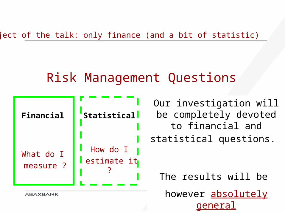
Subject of the talk: only finance (and a bit of statistic)

Risk Management Questions

Financial Statistical ProbabilisticComputation

al

What do I measure ?

How do I estimate it ?

What hypotheses

should I make ?

How can I carry out the computation

(in time) ?

Our investigation will be completely devoted to financial and statistical

questions.

The results will be

however absolutely general

Part 1:

Defining a Risk Measure

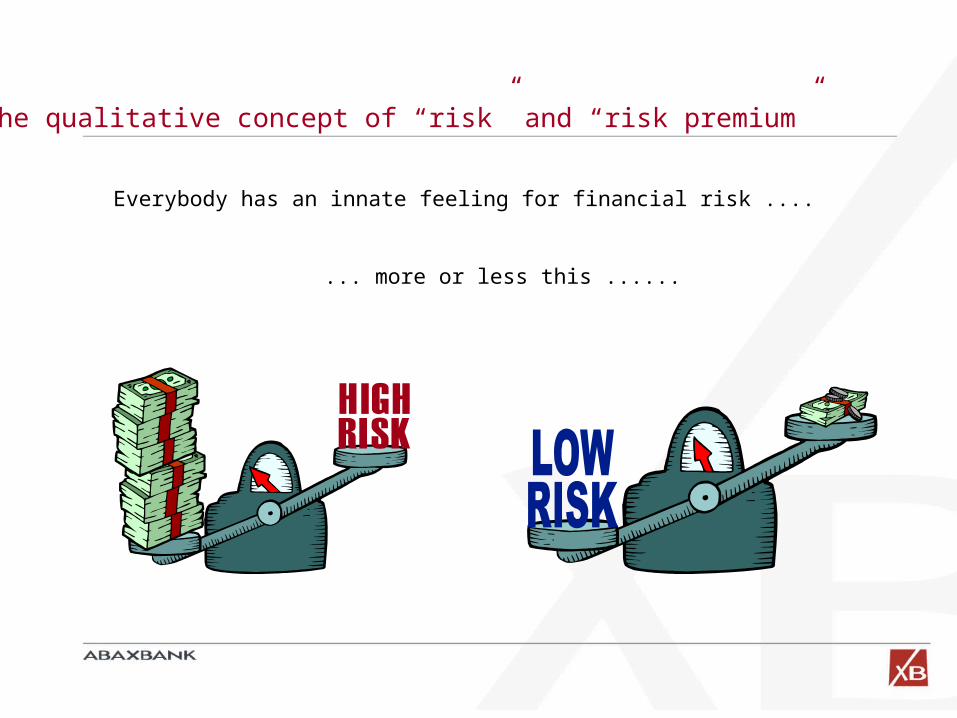
The qualitative concept of “risk” and “risk premium”

Everybody has an innate feeling for financial risk ....

... more or less this ......

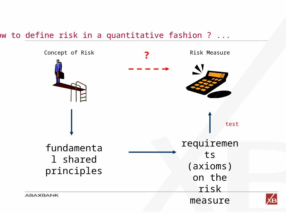
How to define risk in a quantitative fashion ? ...

fundamental shared

principles

requirements (axioms) on the risk measure

Concept of Risk Risk Measure?

test

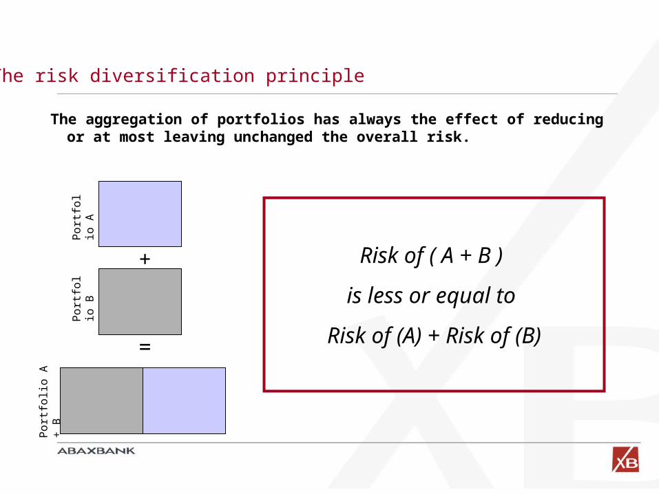
The risk diversification principle

The aggregation of portfolios has always the effect of reducing or at most leaving unchanged the overall risk.

+

=

Port

folio

A

Port

folio

B

Port

folio

A +

B

Risk of ( A + B )

is less or equal to

Risk of (A) + Risk of (B)

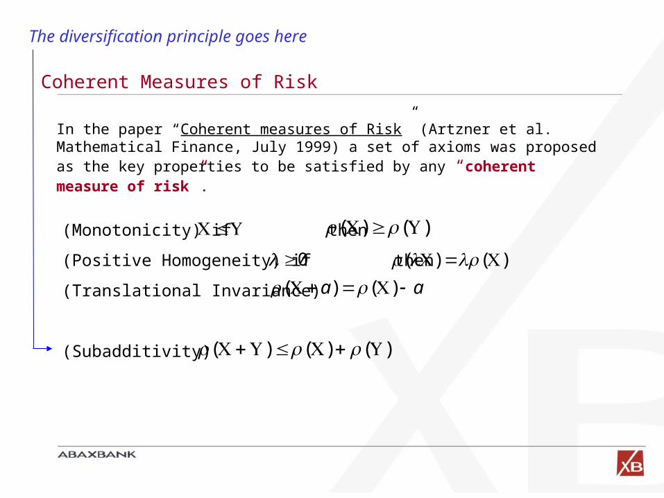
Coherent Measures of Risk

(Monotonicity) if then

(Positive Homogeneity) if then

(Translational Invariance)

(Subadditivity)

)()(

)()()(

0 )()( aa )()(

In the paper “Coherent measures of Risk” (Artzner et al. Mathematical Finance, July 1999) a set of axioms was proposed as the key properties to be satisfied by any “coherent measure of risk”.

The diversification principle goes here

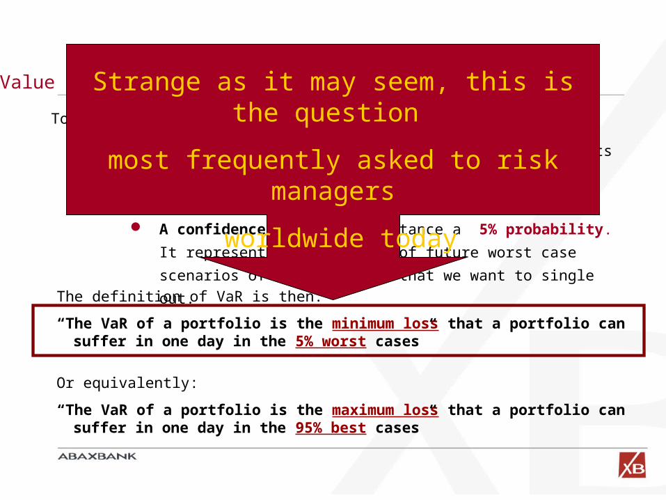
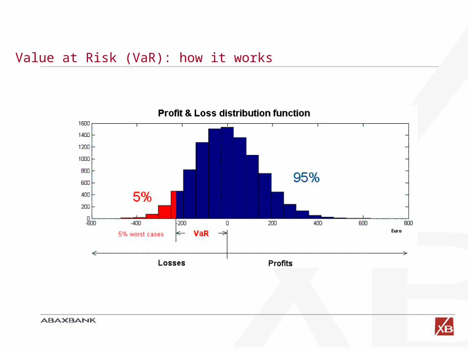
Value at Risk (VaR): how it works

To compute VaR, we need to specify

A time horizon: for instance one day. It represents the

future period over which we measure the risks of a portfolio

A confidence level: for instance a 5% probability. It

represents the fraction of future worst case scenarios of the

portfolio that we want to single out.

The definition of VaR is then:

“The VaR of a portfolio is the minimum loss that a portfolio can suffer in one day in the 5% worst cases”

Strange as it may seem, this is the question

most frequently asked to risk managers

worldwide today

Or equivalently:

“The VaR of a portfolio is the maximum loss that a portfolio can suffer in one day in the 95% best cases”

Value at Risk (VaR): how it works

The formidable advantages introduced by VaR

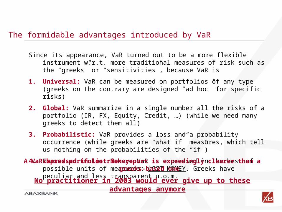
Since its appearance, VaR turned out to be a more flexible instrument w.r.t. more traditional measures of risk such as the “greeks” or “sensitivities”, because VaR is

1. Universal: VaR can be measured on portfolios of any type (greeks on the contrary are designed “ad hoc” for specific risks)

2. Global: VaR summarize in a single number all the risks of a portfolio (IR, FX, Equity, Credit, …) (while we need many greeks to detect them all)

3. Probabilistic: VaR provides a loss and a probability occurrence (while greeks are “what if” measures, which tell us nothing on the probabilities of the “if”)

4. Expressed in Lost Money: VaR is expressed in the best of possible units of measures: LOST MONEY. Greeks have peculiar and less transparent u.o.m.

A VaR-based portfolio risk report is exceedingly clearer than a greeks-based one

No practitioner in 2003 would ever give up to these advantages anymore

The deadly sin of VaR

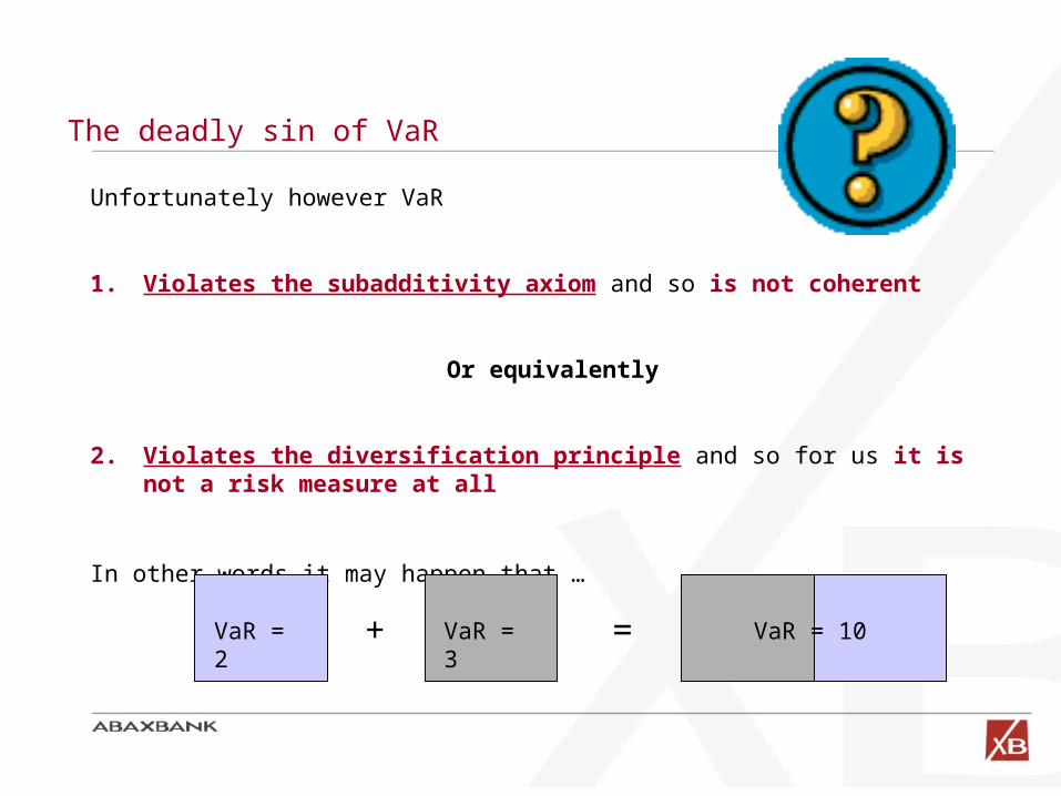
Unfortunately however VaR

1. Violates the subadditivity axiom and so is not coherent

Or equivalently

2. Violates the diversification principle and so for us it is not a risk measure at all

In other words it may happen that …

+ =VaR = 2

VaR = 3

VaR = 10

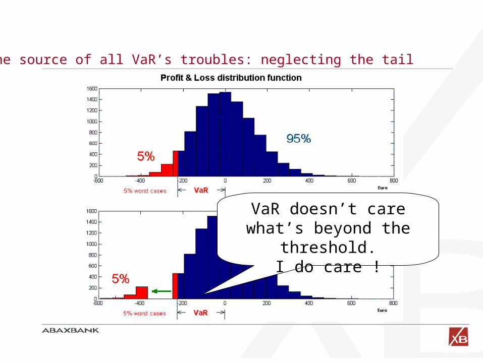
The source of all VaR’s troubles: neglecting the tail

VaR doesn’t care what’s beyond the

threshold.I do care !

Subadditivity and capital allocation

BANK

business unit: Fixed

Income

business unit:

Equities

business unit: Forex

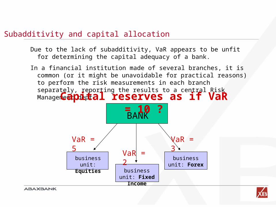
Due to the lack of subadditivity, VaR appears to be unfit for determining the capital adequacy of a bank.

In a financial institution made of several branches, it is common (or it might be unavoidable for practical reasons) to perform the risk measurements in each branch separately, reporting the results to a central Risk Management dept.

VaR = 5

VaR = 3

VaR = 2

Capital reserves as if VaR = 10 ?

What is the concept of risk of VaR ?

From an epistemologic point of view however,

the main problem of VaR is not its lack of subadditivity

but the very lack of any associated consistent set of axioms

We still wonder what concept of risk Value at Risk has in mind !

A natural question

Is it possible to find coherent measures which are as versatile and flexible as VaR ?

The answer is fortunately YES

(… and they are also infinitely many …)

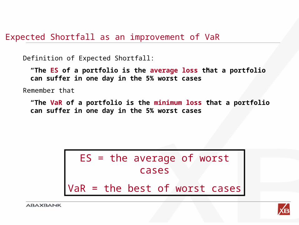
Expected Shortfall as an improvement of VaR

Definition of Expected Shortfall:

“The ES of a portfolio is the average loss that a portfolio can suffer in one day in the 5% worst cases”

Remember that

“The VaR of a portfolio is the minimum loss that a portfolio can suffer in one day in the 5% worst cases”

ES = the average of worst cases

VaR = the best of worst cases

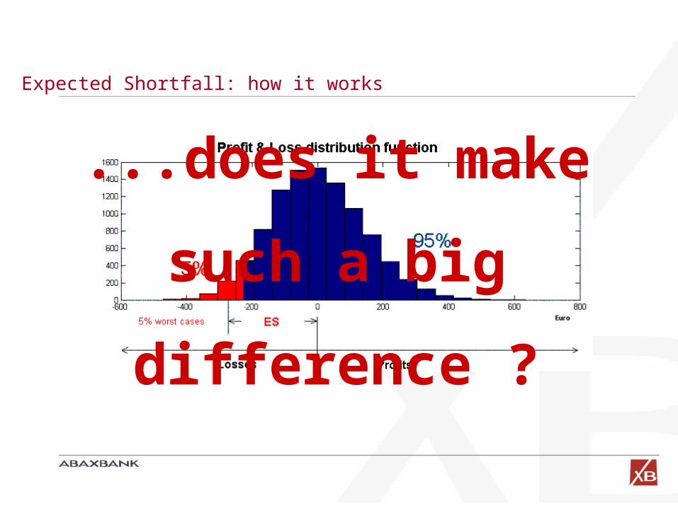
Expected Shortfall: how it works

...does it make

such a big

difference ?

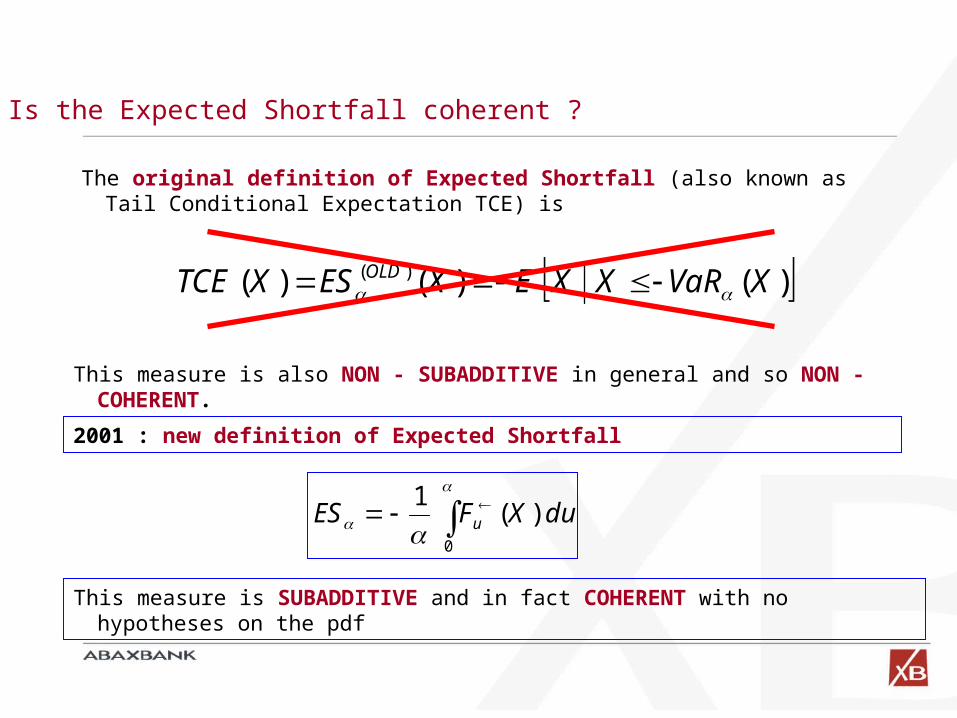
Is the Expected Shortfall coherent ?

)()()( )( XVaRXXEXESXTCE OLD

The original definition of Expected Shortfall (also known as Tail Conditional Expectation TCE) is

This measure is also NON - SUBADDITIVE in general and so NON - COHERENT.

2001 : new definition of Expected Shortfall

duXFES u )(1

0

This measure is SUBADDITIVE and in fact COHERENT with no hypotheses on the pdf

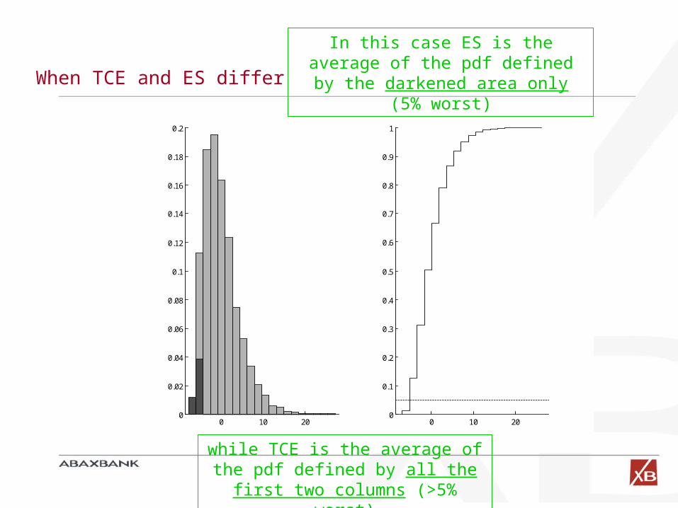
When TCE and ES differ

0 10 200

0.02

0.04

0.06

0.08

0.1

0.12

0.14

0.16

0.18

0.2

0 10 200

0.1

0.2

0.3

0.4

0.5

0.6

0.7

0.8

0.9

1

while TCE is the average of the pdf defined by all the first two

columns (>5% worst)

In this case ES is the average of the pdf defined by the darkened

area only (5% worst)

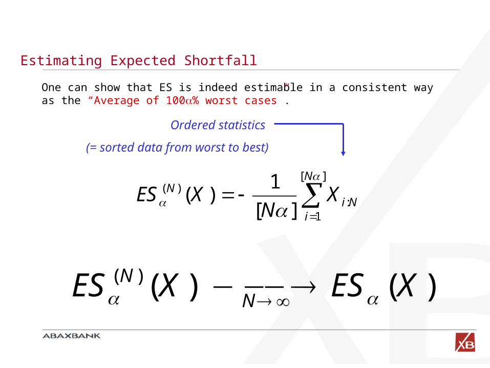
Estimating Expected Shortfall

][

1:

)(

][

1)(

N

iNi

N XN

XES

One can show that ES is indeed estimable in a consistent way as the “Average of 100% worst cases”.

Ordered statistics

(= sorted data from worst to best)

)()()( XESXESN

N

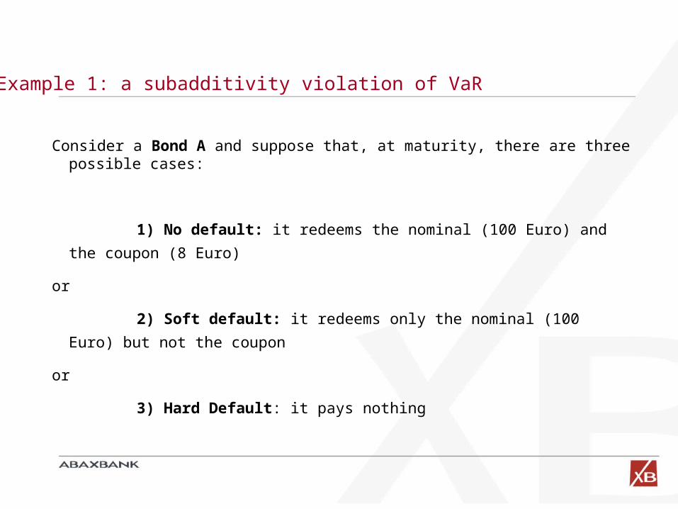
Example 1: a subadditivity violation of VaR

Consider a Bond A and suppose that, at maturity, there are three possible cases:

1) No default: it redeems the nominal (100 Euro) and the

coupon (8 Euro)

or

2) Soft default: it redeems only the nominal (100 Euro) but not

the coupon

or

3) Hard Default: it pays nothing

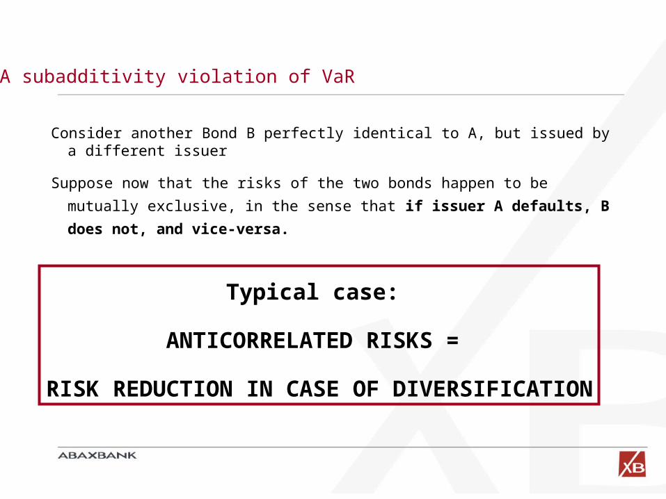
A subadditivity violation of VaR

Consider another Bond B perfectly identical to A, but issued by a different issuer

Suppose now that the risks of the two bonds happen to be mutually

exclusive, in the sense that if issuer A defaults, B does not, and vice-

versa.

Typical case:

ANTICORRELATED RISKS =

RISK REDUCTION IN CASE OF DIVERSIFICATION

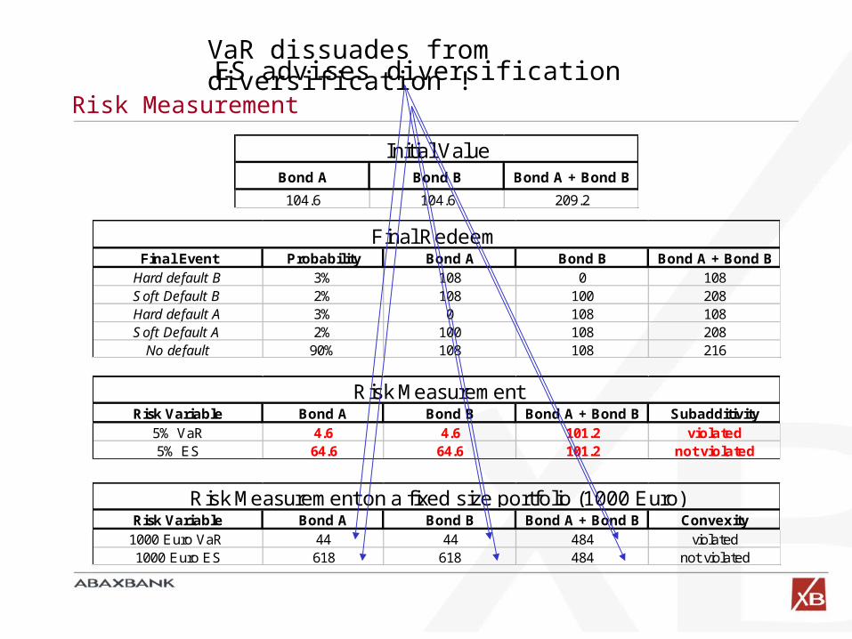
Risk Measurement

Final Event Probability Bond A Bond B Bond A + Bond BHard default B 3% 108 0 108Soft Default B 2% 108 100 208Hard default A 3% 0 108 108Soft Default A 2% 100 108 208

No default 90% 108 108 216

Final Redeem

Bond A Bond B Bond A + Bond B

104.6 104.6 209.2

Initial Value

Risk Variable Bond A Bond B Bond A + Bond B Subadditivity5% VaR 4.6 4.6 101.2 violated5% ES 64.6 64.6 101.2 not violated

Risk Measurement

Risk Variable Bond A Bond B Bond A + Bond B Convexity1000 Euro VaR 44 44 484 violated1000 Euro ES 618 618 484 not violated

Risk Measurement on a fixed size portfolio (1000 Euro)

VaR dissuades from diversification !ES advises diversification

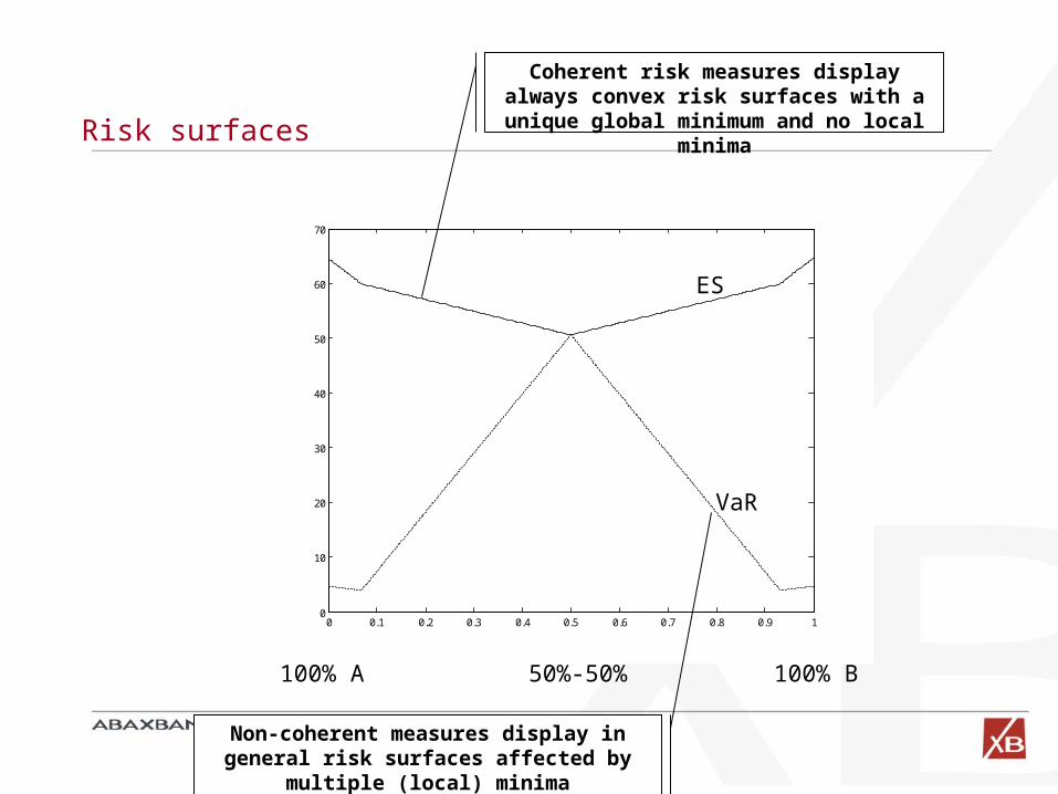
Risk surfaces

0 0.1 0.2 0.3 0.4 0.5 0.6 0.7 0.8 0.9 10

10

20

30

40

50

60

70

100% A 100% B50%-50%

VaR

ES

Coherent risk measures display always convex risk surfaces with a

unique global minimum and no local minima

Non-coherent measures display in general risk surfaces affected by

multiple (local) minima

Example 2: a simple prototype portfolio

Consider a portfolio made of n risky bonds all of which have a 3% default probability and suppose for simplicity that all the default probabilities are independent of one another.

Portfolio = { 100 Euro invested in n independent identical distributed Bonds }

Bond payoff = Nominal (or 0 with probability 3%)

Question: let’s choose n in such a way to minimize the risk of the portfolio

Let’s try to answer this question with a 5% VaR, ES and TCE (= ES (old)) with a time horizon equal to the maturity of the bond.

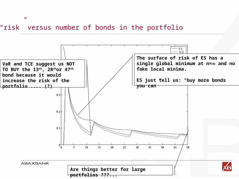
0 5 10 15 20 25 30 35 40 45 500

0.1

0.2

0.3

0.4

0.5

ESTCEVaR

“risk” versus number of bonds in the portfolio

VaR and TCE suggest us NOT TO BUY the 13th, 28thor 47th

bond because it would increase the risk of the portfolio .... (?)

The surface of risk of ES has a single global minimum at n= and no fake local minima.

ES just tell us: “buy more bonds you can”

Are things better for large portfolios ???...

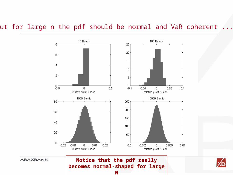
...but for large n the pdf should be normal and VaR coherent ... (!!!)

Notice that the pdf really becomes normal-shaped for

large N

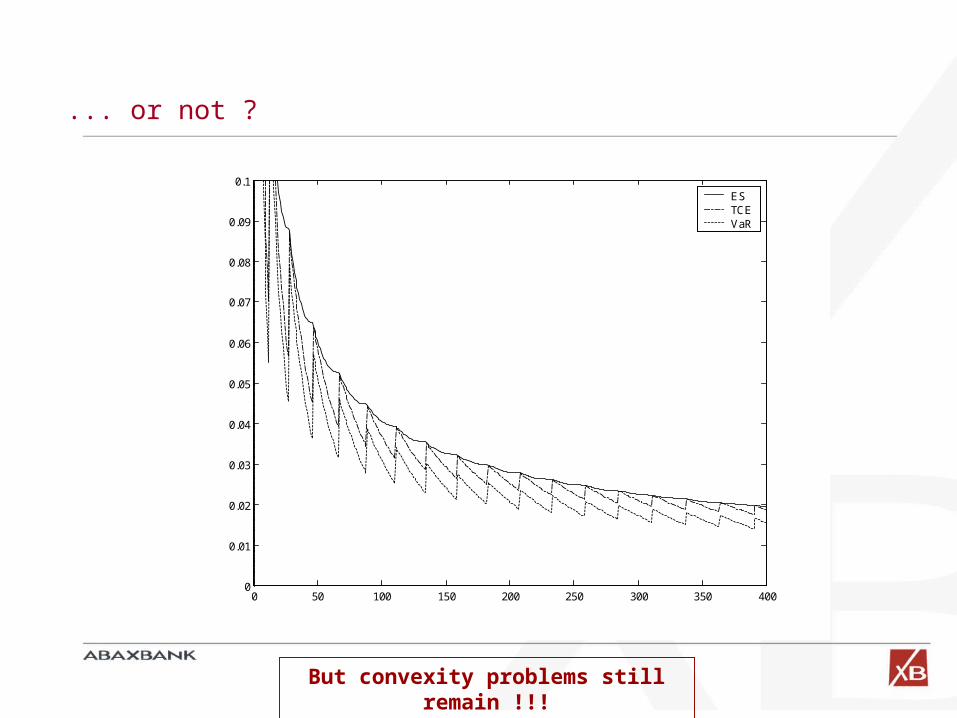
... or not ?

0 50 100 150 200 250 300 350 4000

0.01

0.02

0.03

0.04

0.05

0.06

0.07

0.08

0.09

0.1ESTCEVaR

But convexity problems still remain !!!

Part 2:

Defining a space of risk measures

A natural question: ... other coherent measures ?

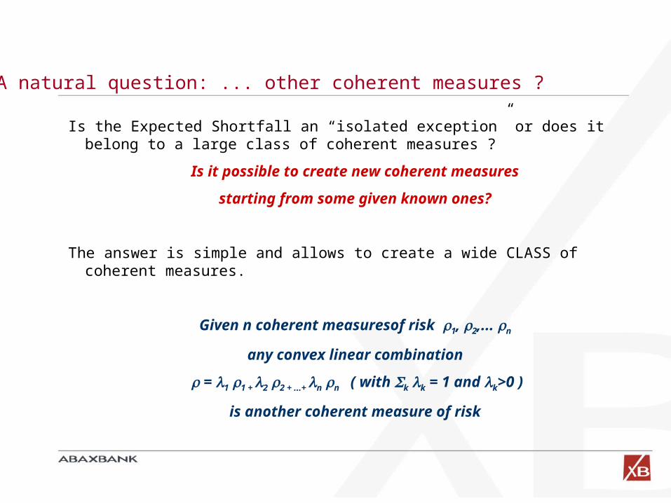
Is the Expected Shortfall an “isolated exception” or does it belong to a large class of coherent measures ?

Is it possible to create new coherent measures

starting from some given known ones?

The answer is simple and allows to create a wide CLASS of coherent measures.

Given n coherent measuresof risk 1, 2,... n

any convex linear combination

= 1 1 + 2 2 + ...+ n n ( with k k = 1 and k>0 )

is another coherent measure of risk

Geometrical interpretation

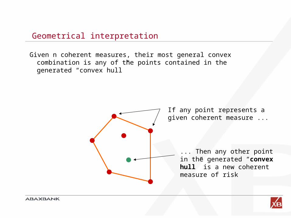
If any point represents a given coherent measure ...

... Then any other point in the generated “convex hull” is a new coherent measure of risk

Given n coherent measures, their most general convex combination is any of the points contained in the generated “convex hull”

Our strategy ....

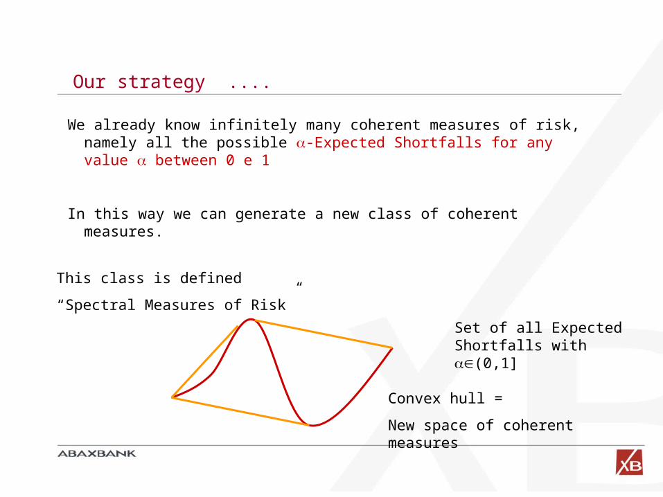
Set of all Expected Shortfalls with (0,1]

Convex hull =

New space of coherent measures

We already know infinitely many coherent measures of risk, namely all the possible -Expected Shortfalls for any value between 0 e 1

In this way we can generate a new class of coherent measures.

This class is defined

“Spectral Measures of Risk”

Spectral measures of risk: explicit characterization

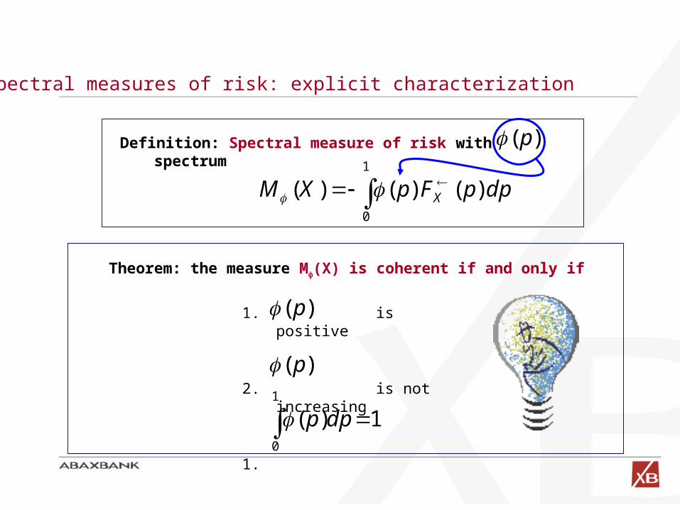
Definition: Spectral measure of risk with spectrum

1

0

)()()( dppFpXM X

)( p

Theorem: the measure M(X) is coherent if and only if

1. is positive

2. is not increasing

1.

)( p

)( p

1)(1

0

dpp

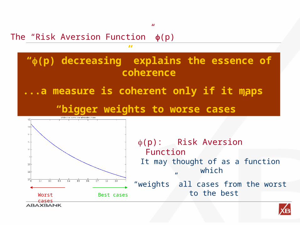
The “Risk Aversion Function” (p)

Any admissible (p) represents a possible legitimate rational attitude toward risk

A rational investor may express her own subjective risk aversion through her own subjective (p) which in turns give her own spectral

measure M

(p): Risk Aversion Function

Best cases Worst cases

It may thought of as a function which

“weights” all cases from the worst to the best

“(p) decreasing” explains the essence of coherence

...a measure is coherent only if it maps

“bigger weights to worse cases”

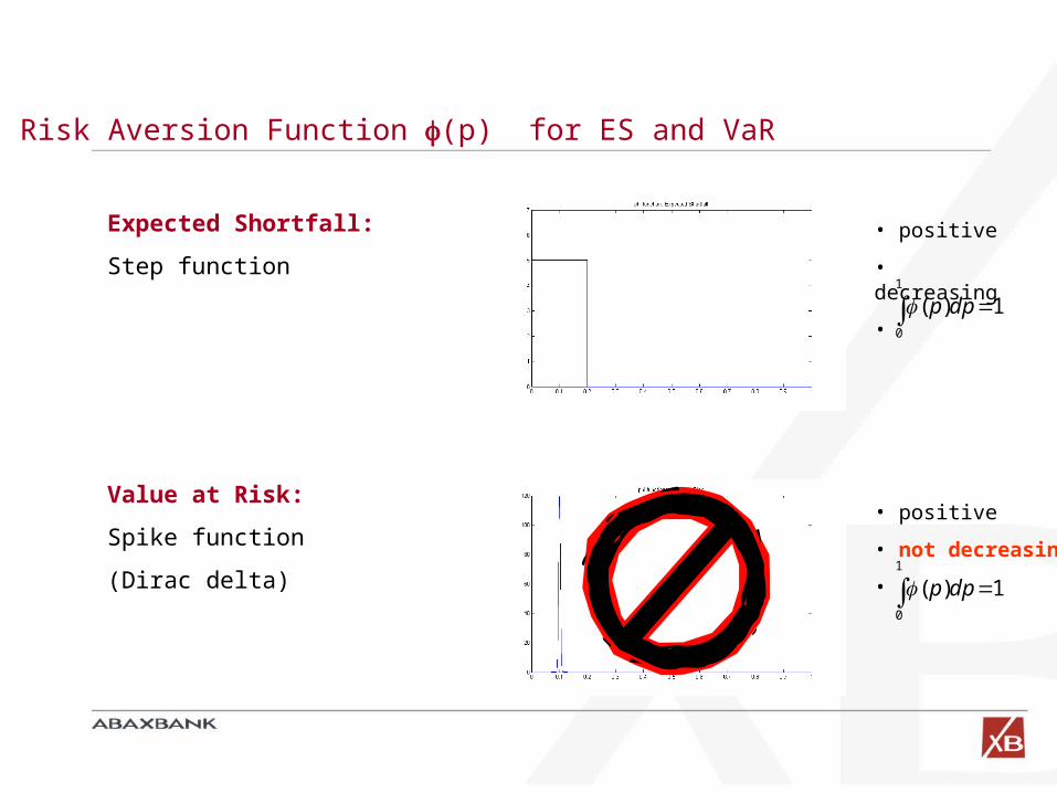
Risk Aversion Function (p) for ES and VaR

Expected Shortfall:

Step function

• positive

• decreasing

• 1)(1

0

dpp

Value at Risk:

Spike function

(Dirac delta)

• positive

• not decreasing

• 1)(1

0

dpp

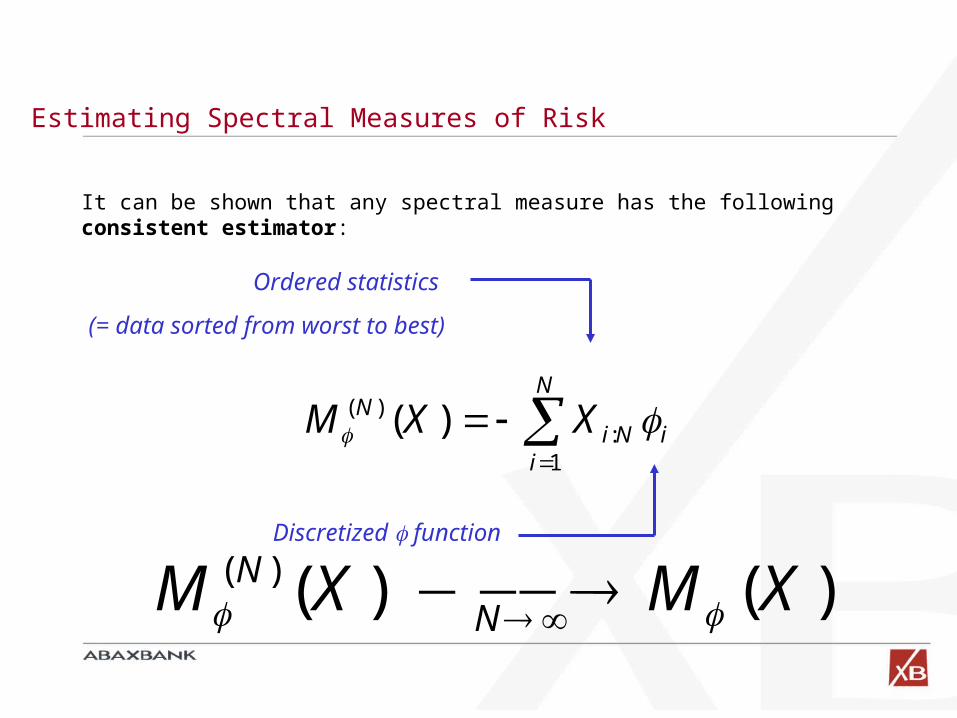
Estimating Spectral Measures of Risk

N

iiNi

N XXM1

:)( )(

It can be shown that any spectral measure has the following consistent estimator:

Discretized function

Ordered statistics

(= data sorted from worst to best)

)()()( XMXMN

N

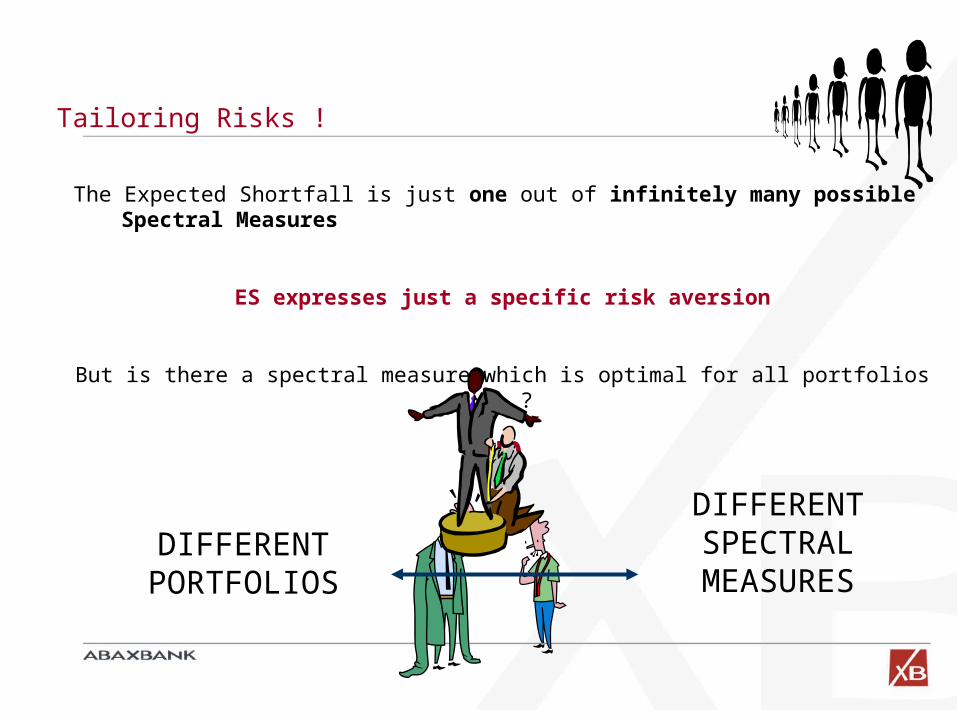
Tailoring Risks !

The Expected Shortfall is just one out of infinitely many possible Spectral Measures

ES expresses just a specific risk aversion

But is there a spectral measure which is optimal for all portfolios ?

NO

DIFFERENT PORTFOLIOS

DIFFERENT SPECTRAL MEASURES

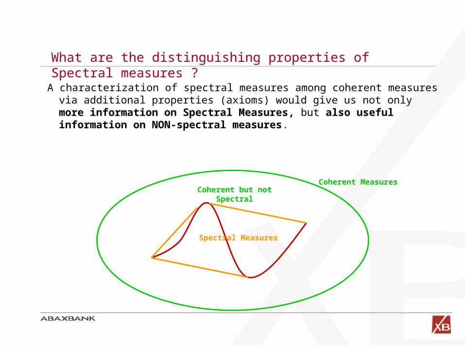
What are the distinguishing properties of Spectral measures ?

A characterization of spectral measures among coherent measures via additional properties (axioms) would give us not only more information on Spectral Measures, but also useful information on NON-spectral measures.

Coherent Measures

Spectral Measures

Coherent but not Spectral

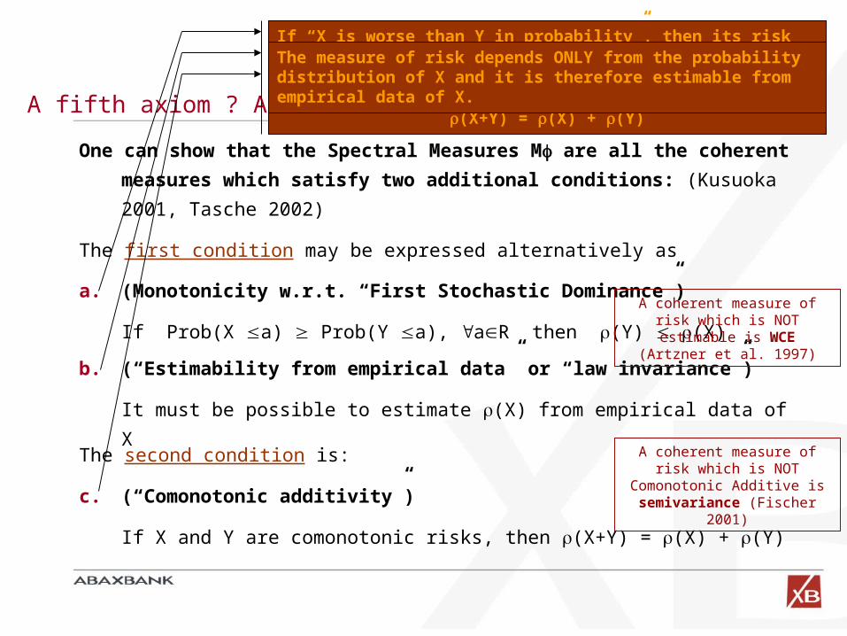
A fifth axiom ? A sixth one ?

One can show that the Spectral Measures M are all the coherent

measures which satisfy two additional conditions: (Kusuoka

2001, Tasche 2002)

The first condition may be expressed alternatively as

The second condition is:

c. (“Comonotonic additivity”)

If X and Y are comonotonic risks, then (X+Y) = (X) + (Y)

a. (Monotonicity w.r.t. “First Stochastic Dominance”)

If Prob(X a) Prob(Y a), aR then (Y) (X)

b. (“Estimability from empirical data” or “law invariance”)

It must be possible to estimate (X) from empirical data of X

If X and Y are “perfectly correlated”, then the risk of X+Y must be the sum of the risks of X and Y.

(X+Y) = (X) + (Y)

If “X is worse than Y in probability”, then its risk must be biggerThe measure of risk depends ONLY from the probability distribution of X and it is therefore estimable from empirical data of X.

A coherent measure of risk which is NOT estimable is WCE (Artzner et al. 1997)

A coherent measure of risk which is NOT Comonotonic Additive is semivariance

(Fischer 2001)

Part 3:

A wider class: Convex Measures of Risk

Handle with care

Liquidity Risk: when coherency violations make sense

When an asset position in a portfolio has a size which is comparable with the capacity of the market (market depth) of absorbing a sudden sell off, we are in presence of liquidity risk. Selling large asset amounts moves market bids downwards.

In this case clearly

Risk (A+A) = Risk (2 A) > 2 Risk (A) = Risk(A) + Risk (A)

Subadditivity fails )()()(

Positive Homogeneity fails 0 )()(

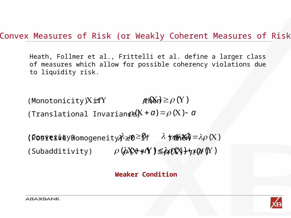
Convex Measures of Risk (or Weakly Coherent Measures of Risk)

(Monotonicity) if then

(Translational Invariance)

)()( aa )()(

Heath, Follmer et al., Frittelli et al. define a larger class of measures which allow for possible coherency violations due to liquidity risk.

(Positive Homogeneity) if then

(Subadditivity) )()()( 0 )()( (Convexity)

)()()(

10,

Weaker Condition

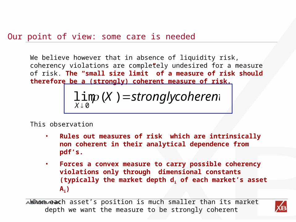
Our point of view: some care is needed

We believe however that in absence of liquidity risk, coherency violations are completely undesired for a measure of risk. The “small size limit” of a measure of risk should therefore be a (strongly) coherent measure of risk.

coherentstronglyXX

)(lim0

This observation

• Rules out measures of risk which are intrinsically non coherent in their analytical dependence from pdf’s.

• Forces a convex measure to carry possible coherency violations only through dimensional constants (typically the market depth di of each market’s asset Ai)

When each asset’s position is much smaller than its market depth we want the measure to be strongly coherent

Convex measures: a step forward ?

We are persuaded that convex measures of risk may represent a significant step forward in risk market practice provided that they respect the “small size coherent limit”. Otherwise, trying to take liquidity into account we may jeopardize the properties of coherency where it should hold in a strong sense.

A convex measure “beyond coherency” is therefore typically NOT a smarter formula which allows coherency violations, because it should be sensitive to positions sizes.

A convex measure “beyond coherency” is more probably a measure with a coherent analytical structure PLUS a database of each assets’ market depths to which the position sizes have to be compared in the search for illiquidities.

A natural solution

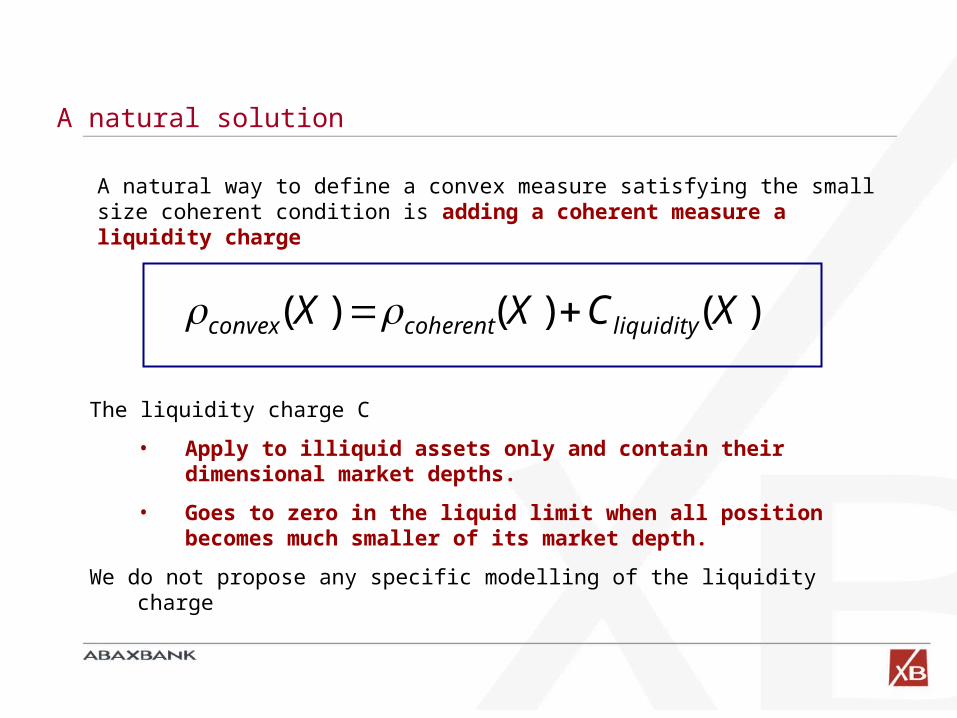
A natural way to define a convex measure satisfying the small size coherent condition is adding a coherent measure a liquidity charge

)()()( XCXX liquiditycoherentconvex

The liquidity charge C

• Apply to illiquid assets only and contain their dimensional market depths.

• Goes to zero in the liquid limit when all position becomes much smaller of its market depth.

We do not propose any specific modelling of the liquidity charge

Part 4:

Coherency and convexity: optimizing spectral measures

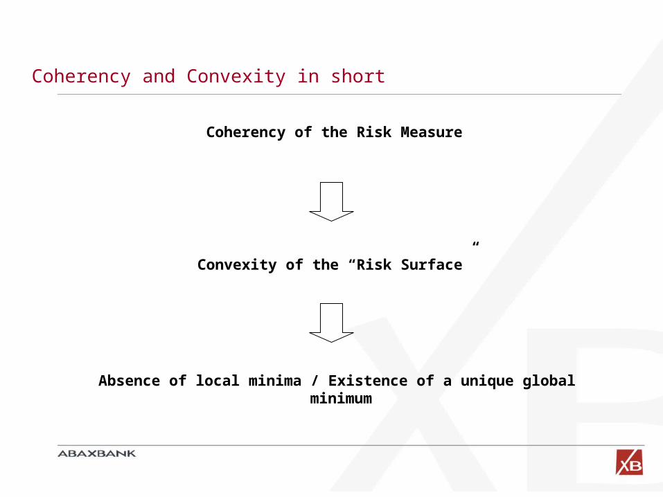
Coherency and Convexity in short

Coherency of the Risk Measure

Convexity of the “Risk Surface”

Absence of local minima / Existence of a unique global minimum

Minimizing the Expected Shortfall

][

1:

)( )(][

1min))((min

N

iNi

w

N

wwX

NwXES

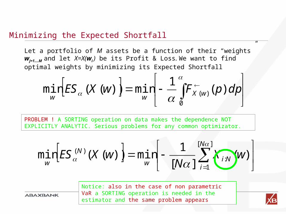
Let a portfolio of M assets be a function of their “weights” wj=1....M and let X=X(wi ) be its Profit & Loss. We want to find optimal weights by minimizing its Expected Shortfall

In the case of a N scenarios estimator we have

0

)( )(1

min))((min dppFwXES wXww

Notice: also in the case of non parametric VaR a SORTING operation is needed in the estimator and the same problem appears

PROBLEM ! A SORTING operation on data makes the dependence NOT EXPLICITLY ANALYTIC. Serious problems for any common optimizator.

The Pflug-Uryasev-Rockafellar solution

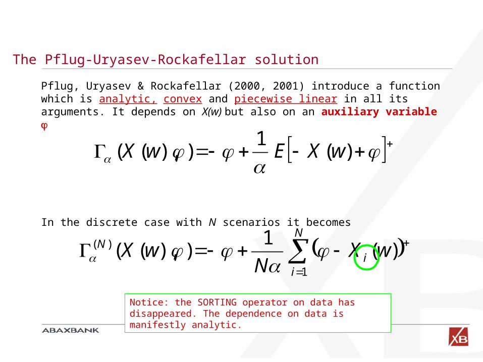
Pflug, Uryasev & Rockafellar (2000, 2001) introduce a function which is analytic, convex and piecewise linear in all its arguments. It depends on X(w) but also on an auxiliary variable

In the discrete case with N scenarios it becomes

)(1

)),(( wXEwX

N

ii

N wXN

wX1

)( )(1

)),((

Notice: the SORTING operator on data has disappeared. The dependence on data is manifestly analytic.

Properties of : the Pflug-Uryasev-Rockafellar theorem

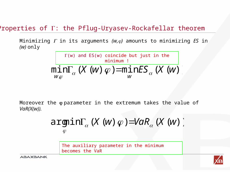
Minimizing in its arguments (w,) amounts to minimizing ES in (w) only

Moreover the parameter in the extremum takes the value of VaR(X(w)).

))((min)),((min,

wXESwXww

))(()),((minarg wXVaRwX

The auxiliary parameter in the minimum becomes the VaR

(w) and ES(w) coincide but just in the minimum !

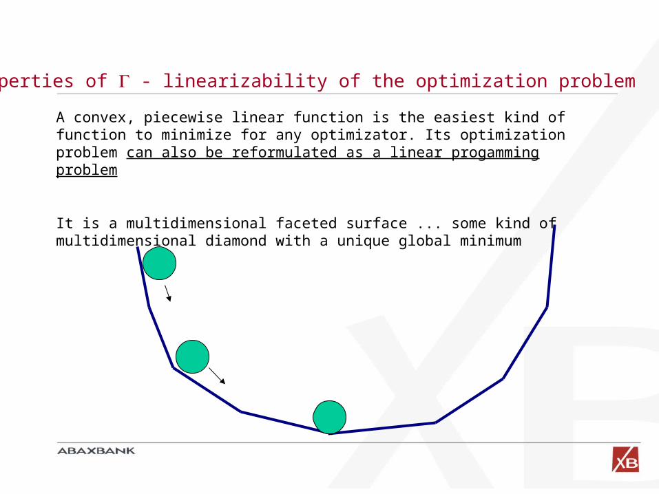
Properties of - linearizability of the optimization problem

A convex, piecewise linear function is the easiest kind of function to minimize for any optimizator. Its optimization problem can also be reformulated as a linear progamming problem

It is a multidimensional faceted surface ... some kind of multidimensional diamond with a unique global minimum

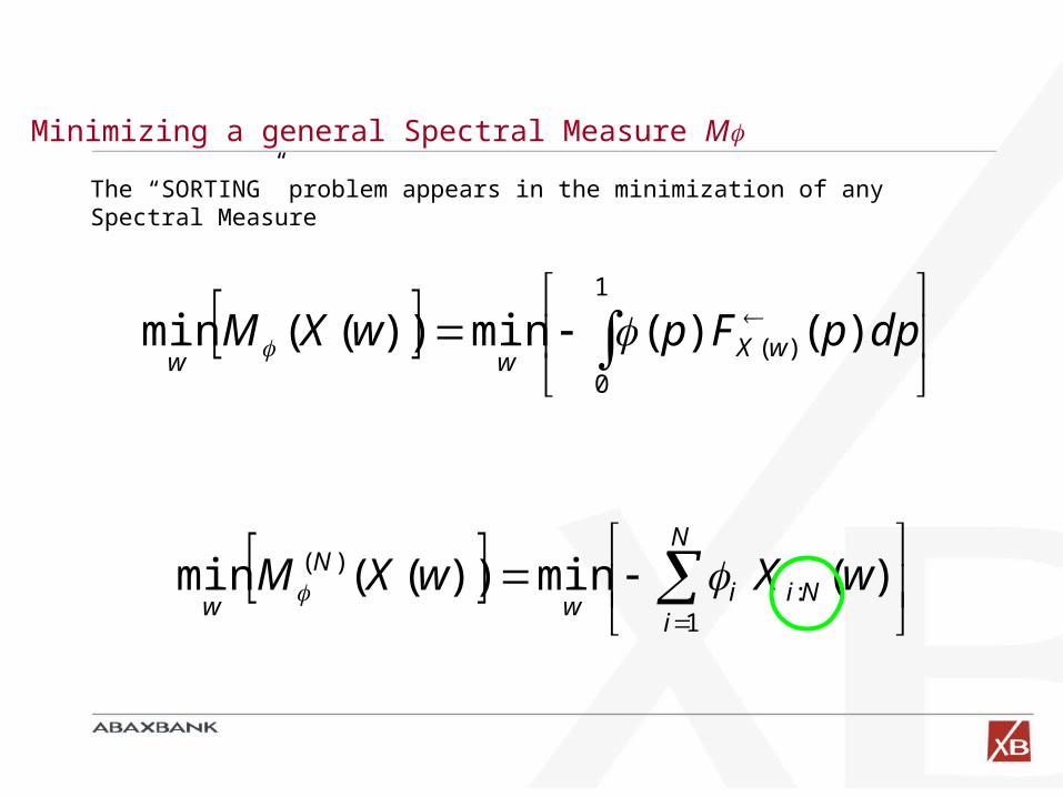
Minimizing a general Spectral Measure M

N

iNii

w

N

wwXwXM

1:

)( )(min))((min

The “SORTING” problem appears in the minimization of any Spectral Measure

1

0

)( )()(min))((min dppFpwXM wXww

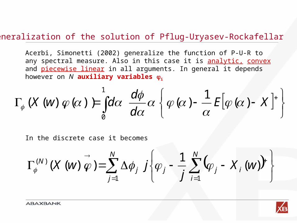
Generalization of the solution of Pflug-Uryasev-Rockafellar

Acerbi, Simonetti (2002) generalize the function of P-U-R to any spectral measure. Also in this case it is analytic, convex and piecewise linear in all arguments. In general it depends however on N auxiliary variables i

In the discrete case it becomes

1

0

)(1

)())(),(( XEd

ddwX

N

iijj

N

jj

N wXj

jwX11

)( )(1

)),((

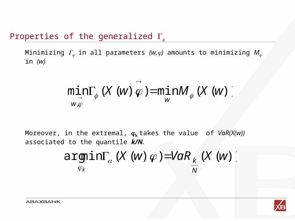
Properties of the generalized

Minimizing in all parameters (w,) amounts to minimizing M in (w)

Moreover, in the extremal, k takes the value of VaR(X(w)) associated to the quantile k/N.

))((min)),((min,

wXMwXw

w

))(()),((minarg wXVaRwXN

kk

Part 5:

Some hints for an internal model ?

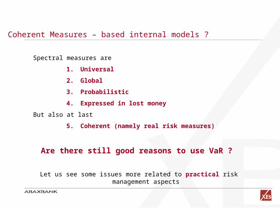
Coherent Measures – based internal models ?

Spectral measures are

1. Universal

2. Global

3. Probabilistic

4. Expressed in lost money

But also at last

5. Coherent (namely real risk measures)

Are there still good reasons to use VaR ?

Let us see some issues more related to practical risk management aspects

Spectral Measures: worse statistical properties ?

Definitely not

1. The statistical error of Spectral Measures is easily computable and is by no means worse in general than VaR’s (Acerbi, Meucci, Tasche: in preparation).

2. It is not true that “ES is Extreme Value Theory and VaR not”. They are probably both EVT in most cases, and this depend mostly on the size of the chosen confidence levels.

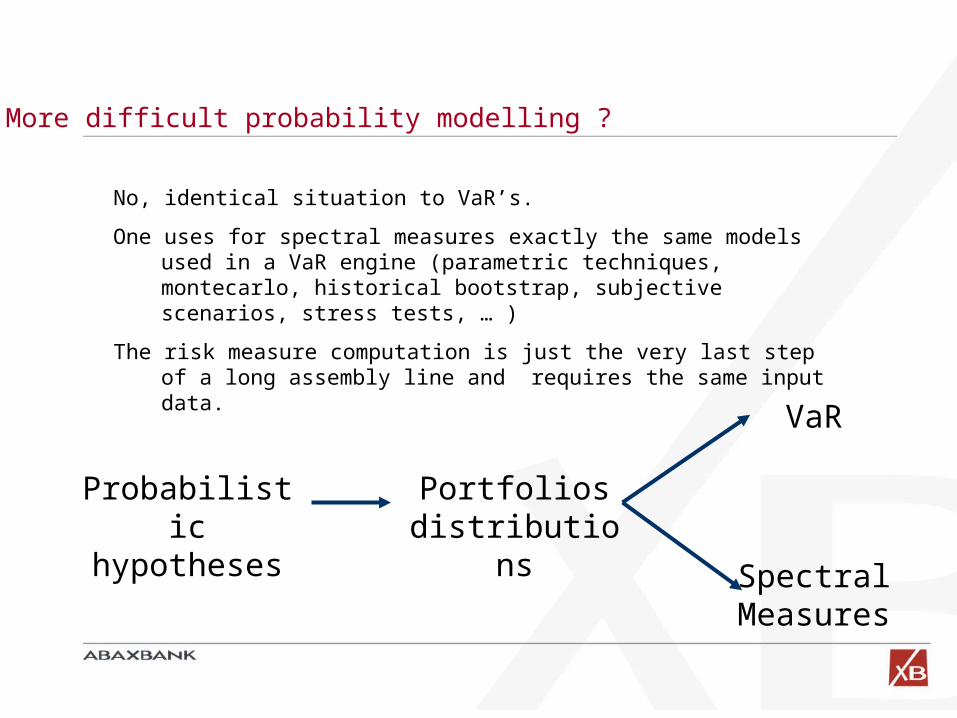
More difficult probability modelling ?

No, identical situation to VaR’s.

One uses for spectral measures exactly the same models used in a VaR engine (parametric techniques, montecarlo, historical bootstrap, subjective scenarios, stress tests, … )

The risk measure computation is just the very last step of a long assembly line and requires the same input data.

Probabilistic hypotheses

Portfolios distributions

VaR

Spectral Measures

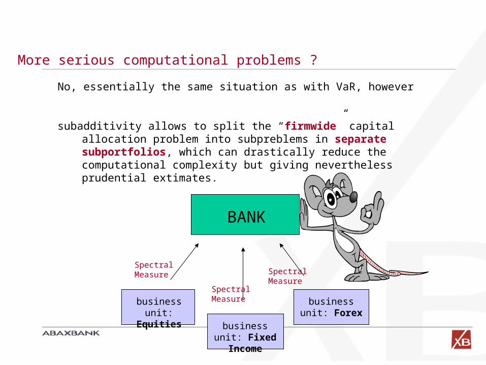
More serious computational problems ?

No, essentially the same situation as with VaR, however

subadditivity allows to split the “firmwide” capital allocation problem into subpreblems in separate subportfolios, which can drastically reduce the computational complexity but giving nevertheless prudential extimates.

BANK

business unit: Fixed

Income

business unit:

Equities

business unit: Forex

Spectral Measure

Spectral Measure

Spectral Measure

Optimization is more difficult ?

The contrary is certainly true !

Coherence in optimization problems implies convexity of risk measures.

Optimizing VaR on a portfolio of 100 assets may turn out to be a formidable NON-CONVEX problem of huge complexity.

Optimizing a Spectral Measure on a portfolio of thousands of assets is a problem that can always been faced since it is

1. CONVEX

2. LINEARIZABLE

Pflug, Rockafellar, Uryasev, (2000 –2001), Acerbi, Simonetti (2002)

Different Risk Measures in any bank ?

Regulating a bank industry where any bank could in principle use a different risk measure would prompt complications that are beyond the scope of our talk.

We note however that

1. No measure of risk fits any portfolio of a generic financial institution. The risk aversion function is a precision instrument which allows to better detect the risks of portfolios in different business styles (e.g.: insurance portfolios from bank portfolios …).

2. The possibility of providing market players with different risk measures could cancel the suspect that a unique measure of risk could prompt “flock effects” in the case of market crises.

However, we personally don’t believe that VaR has been a source for systemic risk in recent crises. Panic selling had been invented long

before !!

Conclusions

The space of Spectral Measures M provides the representation of a huge class of coherent measures suitable for applications. Coherent measures which are not spectral display properties which are undesirable in real life finance.

Any coherent measure of this space is in one-to-one correspondence with any possible rational aversion to risk of an investor.

For any spectral measure M a consistent estimator is available based on empirical data.

The practical application of any spectral measure is elementary and the conversion of a VaR engine straightforward.

Optimization of spectral measures is a convex and linearizable problem.

There’s nothing special with ES. It is just one out of infinitely many other spectral measures.