Embed Size (px)
Citation preview
1
Spectral Decomposition of Seismic Data with Continuous
Wavelet Transform
Satish Sinha
School of Geology and Geophysics,
University of Oklahoma, Norman, OK 73019 USA
Partha Routh
Department of Geosciences,
Boise State University, Boise, ID 83725 USA
Phil Anno
Seismic Imaging and Prediction,
ConocoPhillips, Houston, TX 77252 USA
John Castagna
School of Geology and Geophysics,
University of Oklahoma, Norman, OK 73019 USA
(Revision Date: March, 14, 2005)
2
ABSTRACT
In this paper we present a new methodology for computing a time-frequency map
for non-stationary signals using the continuous wavelet transform (CWT). The
conventional method of producing a time-frequency map using the Short Time Fourier
Transform (STFT) limits the time-frequency resolution by a pre-defined window length.
In contrast, the CWT method does not require pre-selecting a window length and does
not have a fixed time-frequency resolution over the time-frequency space. The CWT
utilizes dilation and translation of a wavelet to produce a time-scale map. One scale
encompasses a frequency band, and is inversely proportional to the time support of the
dilated wavelet. Previous workers have converted a time-scale map into a time-frequency
map by taking the center frequencies of each scale. We transform the time-scale map by
taking the Fourier transform of the inverse CWT to produce a time-frequency map. Thus,
a time-scale map is converted into a time-frequency map in which the amplitudes of
individual frequencies rather than frequency bands are represented. We refer to such a
map as the time-frequency CWT (TFCWT).
We validate our approach with a non-stationary synthetic example and compare
the results with the STFT and a typical CWT spectrum. Two field examples illustrate that
the TFCWT can potentially be utilized to detect frequency shadows caused by
hydrocarbons and identify subtle stratigraphic features for reservoir characterization.
3
INTRODUCTION
Seismic data, being non-stationary in nature, have varying frequency content in
time. Time-frequency decomposition, also called spectral decomposition, of a seismic
signal aims to characterize the time-dependent frequency response of subsurface rocks
and reservoirs. Castagna et al. (2003) used matching pursuit decomposition for
instantaneous spectral analysis to detect low frequency shadows beneath hydrocarbon
reservoirs. A case history of using spectral decomposition and coherency to interpret
incised valleys was shown by Peyton et al. (1998). Partyka et al. (1999) used windowed
spectral analysis to produce discrete-frequency energy cubes for applications in reservoir
characterization. Hardy et al. (2003) showed that an average frequency attribute produced
from sine-curve fitting strongly correlates with shale volume in a particular area.
Since time-frequency mapping is a non-unique process, there exist various
methods for time-frequency analysis of non-stationary signals. Jones and Baraniuk
(1995) describe a data-adaptive method that is not addressed in this paper. The first and
widely used method is the short-time Fourier transform (STFT) in which a time-
frequency spectrum is produced by taking the Fourier transform over a chosen time
window (Cohen, 1995). In this method time-frequency resolution is fixed over the entire
time-frequency space by pre-selecting a window length. Therefore, resolution in seismic
data analysis becomes dependent on a user specified window length.
In the past two decades, the wavelet transform has been applied in many branches
of science and engineering. The continuous wavelet transform (CWT) provides a
different approach to time-frequency analysis. Instead of a time-frequency spectrum, it

4
produces a time-scale map called a scalogram (Rioul and Vetterli, 1991). Since scale
represents a frequency band, it is not intuitive if we wish to interpret the frequency
content of the signal. Previous workers (Abry et al., 1993; Hlawatsch and Bartels, 1992)
took scale to be inversely proportional to the center frequency of the wavelet and
represented the scalogram as a time-frequency map.
This paper provides a novel approach for mapping the time-scale map into a time-
frequency map. Time-frequency CWT (TFCWT, Sinha, 2002) analysis provides high
frequency resolution at low frequencies and high time resolution at high frequencies. This
optimal time-frequency resolution property of the TFCWT makes it useful in seismic data
analysis.
Computation of the TFCWT in the Fourier domain is a fast process. Furthermore,
TFCWT is an invertible process such that the inverse Fourier transform of the time
summation of the TFCWT reconstructs the original signal provided the inverse wavelet
transform exists. For our analysis purpose we require only the forward transform and
reproducibility is not a strict requirement.
Seismic data analysts sometimes observe low frequency shadows in association
with hydrocarbon reservoirs. The shadow is probably caused by attenuation of high
frequency energy in the reservoir itself (Mitchell et at., 1996; Dilay and Eastwood, 1995)
such that the local dominant frequency moves towards the low frequency range. Thus,
anomalous low frequency energy is concentrated at or beneath the reservoir level. The
low frequencies are probably not caused by inelastic attenuation. Ebrom (2004) lists
about 10 possible mechanisms. High frequency resolution at low frequencies, given by
the TFCWT, helps detect these shadows. On the other hand, high time resolution at high
5
frequencies can be utilized to enhance stratigraphic features from seismic data. Marfurt
and Kirlin (2001) investigated how tuning frequency varies with thickness and used
spectrally decomposed data to resolve thin beds.
In this paper, we derive a formula to convert a scalogram to a TFCWT and we
begin by comparing the TFCWT spectrum for a hyperbolic chirp signal with the CWT
spectrum and the STFT. Then we calculate TFCWT spectra for two real data sets, one
from Nigeria and another publicly available data set from the Stratton field, South Texas.
In the first example, we show that single frequency visualization of a seismic section in
the frequency domain with the TFCWT reveals low frequency anomalies associated with
hydrocarbon reservoirs. In the second example we show that single frequency slices
along a horizon can be used to enhance stratigraphic features.
TIME-FREQUENCY MAP FROM STFT
The Fourier transform )(ˆ ωf of a signal )(tf is the inner product of the signal
with the basis function tie ω i.e.
∫∞
∞−
−== dtetfetff titi ωωω )(),()(ˆ . (1)
A seismic signal, when transformed into the frequency domain using the Fourier
transform, gives the overall frequency behavior; such a transformation is inadequate for
analyzing a non-stationary signal. We can include the time dependence by windowing the
signal (i.e. taking short segments of the signal) and then performing the Fourier transform
on the windowed data to obtain local frequency information. Such an approach of time-
6
frequency analysis is called the short-time Fourier transform (STFT) and the time-
frequency map is called a spectrogram (Cohen, 1995). The STFT is given by the inner
product of the signal )(tf with a time shifted window function )(tφ . Mathematically, it
can be expressed as:
∫ −−=−= dtettfettfSTFT titi ωω τφτφτω )()()(),(),( , (2)
where the window function φ is centered at time τ=t and φ is the complex conjugate
of φ .
We show a spectrogram computed for a chirp signal (Figure 1) with two
hyperbolic frequency sweeps in Figure 2. We used the “Hanning” window of 400ms
length for this computation. We note in the spectrogram that the low frequencies are well
resolved and the high frequencies are either poorly resolved or not visible at all. The
reason is that the frequency resolution is fixed by the pre-selected window length and it is
recognized as the fundamental problem of the STFT in spectral analysis of a non-
stationary signal.
TIME-FREQUENCY MAP FROM CWT (TFCWT)
The continuous wavelet transform (CWT) is an alternative method to analyze a
signal. In the CWT, wavelets dilate in such a way that the time support changes for
different frequencies. When the time support increases or decreases, the frequency
support of the wavelet is shifted towards high frequencies or low frequencies

7
respectively. Thus, when the frequency resolution increases, the time resolution decreases
and vice-versa (Mallat, 1999).
A wavelet is defined as a function )()( 2 ℜ∈ Ltψ with a zero mean, which is
localized in both time and frequency. By dilating and translating this wavelet )(tψ we
produce a family of wavelets
⎟⎠⎞
⎜⎝⎛ −
=στψ
στψ τσ
t1)(, (3)
where ℜ∈τσ , and 0≠σ . σ is the dilation parameter or scale and τ is the translation
parameter. Note that the wavelet is normalized such that the L2 norm ψ is equal to
unity. The continuous wavelet transform is defined as the inner product of the family of
wavelets )(, tτσψ with the signal )(tf . This is given by
dtttfttfFW ⎟⎠⎞
⎜⎝⎛ −
== ∫∞
∞− στψ
σψτσ τσ
1)()(),(),( , , (4)
where ψ is the complex conjugate of ψ . ),( τσWF is the time-scale map (i.e. the
scalogram). The convolution integral in equation (4) can be easily computed in the
Fourier domain. The choice for the scale and the translation parameter can be arbitrary
and we can chose to represent it any way we like. To reconstruct the function )(tf from
the wavelet transform we use Calderon's identity (Daubechies, 1992), given by,
∫ ∫∞
∞−
∞
∞−
⎟⎠⎞
⎜⎝⎛ −
=στ
σσ
στψτσ
ψ
ddtFC
tf W 2),(1)( . (5)
For the inverse transform to exist we require that the analyzing wavelet satisfy the
"admissibility condition" given by,
8
∫ ∞<= ωωωψ
πψ dC2)(ˆ
2 , (6)
where )(ˆ ωψ is the Fourier transform of )(tψ . The integrand in equation (6) has an
integrable discontinuity at 0=ω and also implies that ∫ = 0)( dttψ . A commonly used
wavelet in continuous wavelet transform is the Morlet wavelet and is defined as
(Torrence and Compo, 1998):
2/4/10
20)( tti eet −−= ωπψ , (7)
where 0ω is the frequency and is taken as π2 to satisfy the admissibility condition. The
center frequency of the Morlet wavelet being inversely proportional to the scale provides
an easy interpretation from scale to frequency.
We note that a scale represents a frequency band and not a single frequency. The
scalogram doesn't provide a direct intuitive interpretation of frequency. In order to
interpret the time-scale map in terms of a time-frequency map a number of approaches
can be taken. The easiest step would be to stretch the scale to an equivalent frequency
depending on the scale-frequency mapping of the wavelet. Typically for time-frequency
analysis one converts a scalogram to a time-frequency spectrum using ff c / where cf is
the center frequency of the wavelet (Hlawatsch and Bartels, 1992). Such a typical CWT
spectrum of the chirp signal using the Morlet wavelet is shown in Figure 3. However, we
take an alternative approach and compute a frequency spectrum of the signal using the
wavelet as an adaptive window. Because of the dilation property of the Morlet wavelet, it
is a natural window for signals that require high frequency resolution at low frequencies
and high time resolution at high frequencies. The translation property allows us to
examine the frequency content at various times, thus leading to a time-frequency map
9
that is adaptive to non-stationary nature of seismic signals, by taking the Fourier
transform of the inverse continuous wavelet transform.
Replacing )(tf from equation (5) into equation (1) gives
∫ ∫ ∫∞
∞−
∞
∞−
∞
∞−
−⎟⎠⎞
⎜⎝⎛ −
= dtddetFC
f tiW τσ
στψτσ
σσω ω
ψ
),(11)(ˆ2
. (8)
Using the scaling and shifting theorem of the Fourier transform, we get
( )σωψσστψ ωτω ˆiti edtet −
∞
∞−
− =⎟⎠⎞
⎜⎝⎛ −
∫ . (9)
By interchanging the integrals and substituting equation (9) in equation (8), we
obtain
∫ ∫∞
∞−
−∞
∞−
= τσσωψστσσσ
ω ωτ
ψ
ddeFC
f iW )(ˆ),(11)(ˆ
2, (10)
where )(ˆ ωψ is the Fourier transform of the mother wavelet.
In order to obtain a time-frequency map we remove the integration over the
translation parameter τ and replace )(ˆ ωf by ),(ˆ τωf . This is given by
2/3)(ˆ),(1),(ˆσσσωψτστω ωτ
ψ
deFC
f iW∫
∞
∞−
−= . (11)
Equation (11) is the fundamental equation that allows us to compute the time-
frequency spectrum from the continuous wavelet transform (TFCWT) of a signal. This
can also be represented as the inner product between the wavelet transform of the signal
),( τσWF and a scaled and modulated window given by )(ˆ σψω , where the scaling is over
the frequency. We note that for a particular frequency we have an appropriately scaled
10
window. The integration in the inner product space is over all scales as denoted by
equation (11). This can be represented by
)(ˆ),,(),(ˆ σψτστω ωWFf = , (12)
where the scaled and modulated window is given by
2/3
)(ˆ)(ˆ
σσωψσψψ
ωτ
ω Ce i−
= , (13)
where )(ˆ σψω is the complex conjugate of )(ˆ σψω . Equation (12) shows that the effective
window is the scaled and modulated wavelet that acts on the transformed signal in the
wavelet domain. In contrast, the chosen window in the STFT directly operates on the
time-domain signal given in equation (2) and the inner product space is integrated over
all times. The time-frequency map generated by equation (11) or equation (12) from the
scalogram ),( τσWF is not obtained by the direct transformation of a scale to its center
frequency, rather this map provides energy at the desired frequency and avoids the
complication of overlapping frequency bands common to a scale-frequency
transformation. Equation (11) can be computed using a two-step procedure. First we
evaluate the convolution integral in equation (4) to obtain ),( τσWF using the Fourier
transform method. In the second step we use the Fourier transformation of the scaled and
modulated wavelet to compute the inner product over all scales. Also note that the time
summation of equation (11) gives the Fourier transform of the signal. Thus,
reconstruction of the original signal is a two-step process: a) time summation of the
TFCWT and b) inverse Fourier transform of the resultant sum.
The synthetic signal (Figure 1) is made up of two hyperbolic sweep frequencies,
each having constant amplitude i.e. energy in each frequency sweep is constant with time.
11
The typical CWT spectrum (Figure 3) for the synthetic signal has improved time-
frequency resolution compared to the STFT spectrum (Figure 2). We note in the CWT
spectrum that the energies in both frequency trends erroneously decrease with increasing
frequency. Considering the fact that the typical CWT spectrum is computed in terms of
frequency bands (i.e. scales) and represented by taking the center frequency of the
frequency bands, these frequency bands overlap each other the overlap increases with
increasing frequency. This results in an apparent loss of energy in the CWT spectrum that
can be confused with attenuation effects which are not present in the signal. However, the
TFCWT spectrum (Figure 4) does not show any erroneous attenuation. The blurring
effect on each end is due to the fact the TFCWT has high frequency resolution and low
time resolution at low frequencies and low frequency resolution and high time resolution
at high frequencies. Thus the TFCWT provides an improved resolution for a non-
stationary signal. In addition to the improvement in the time-frequency resolution, the
new methodology inheriting the CWT avoids the subjective choice of window length
necessary for the STFT.
APPLICATIONS OF TFCWT TO FIELD DATA
Time-frequency spectra produced from the TFCWT can be used to interpret
seismic data in the frequency domain. We have carried out such analyses with post-stack
data sets. Adding a frequency axis to a 2D seismic section makes the data 3D.
Comparison of single frequency sections from such a 3D volume can be utilized to detect
low frequency shadows sometimes caused by hydrocarbon reservoirs. Sun et al. (2002)
12
used instantaneous spectral analysis (ISA) based on matching pursuit decomposition for
direct hydrocarbon detection. A matching pursuit isolates the signal structures that are
coherent with respect to a given wavelet dictionary (Mallat and Zhang, 1993). However,
if the signal is composed of several combinations of fundamental dictionaries, it will be
difficult to choose a particular one to analyze the non-stationary nature. In the TFCWT
time-frequency decomposition is carried out by a mother wavelet. We have noted that the
TFCWT method provides good resolution at low frequencies and is, therefore, effective
in detecting low frequency shadows.
A seismic section from Nigeria data set shown in Figure 5 shows bright
amplitudes (yellow arrows) adjacent to the faults (green arrows) indicative of known
hydrocarbon zones. A preferentially illuminated single frequency section at 20 Hz from
the TFCWT data volume shows high amplitude low frequency anomalies (colored red) at
the reservoir level (yellow arrow) in Figure 6. Furthermore, we observe that at 33 Hz
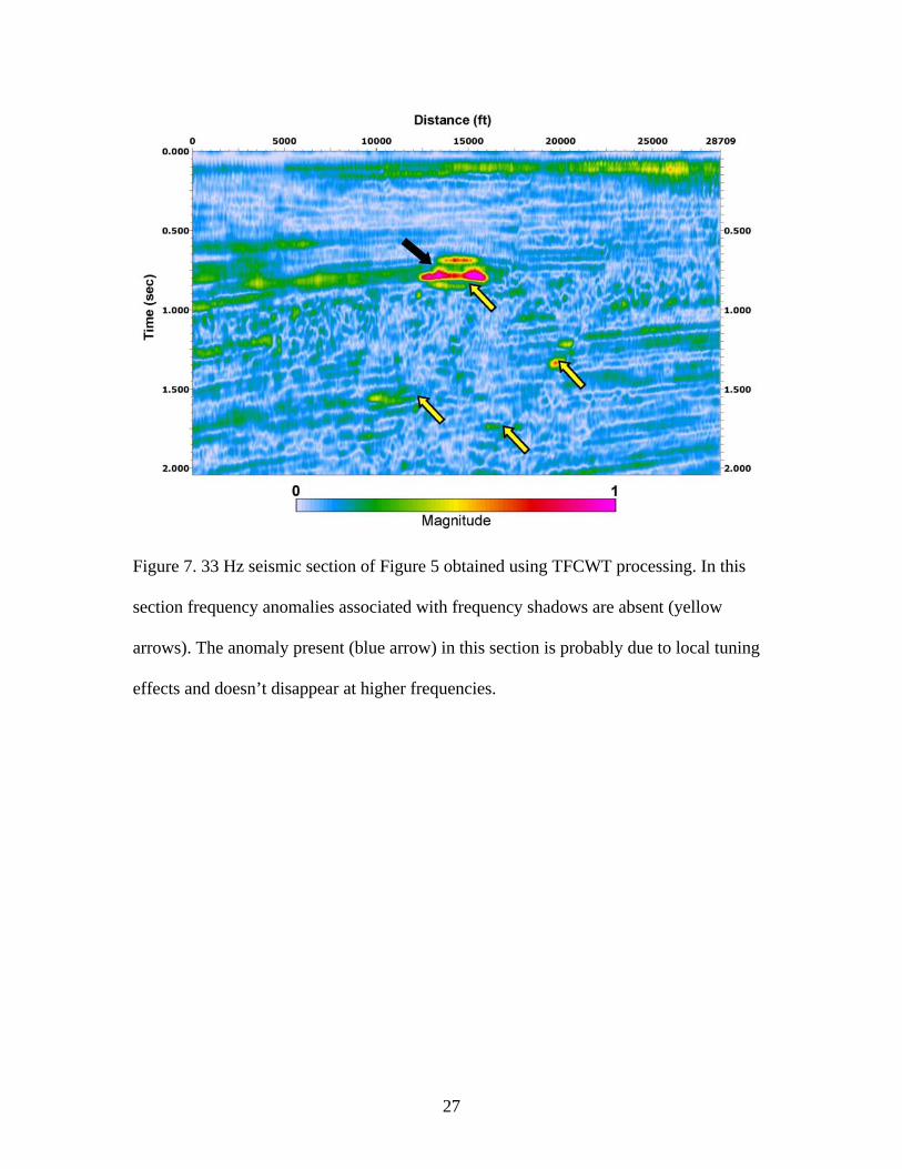
these anomalies disappear as shown in Figure 7. In this example these low frequency
anomalies appear only at the known hydrocarbon reservoirs. Mechanisms for this low
frequency anomaly are not known. Ebrom (2004) suggested 10 possible mechanisms of
frequency shadow effect. The challenge is to determine which are of the first-order
effects, and which are less important. The anomaly above the hydrocarbon reservoir level
(blue arrow) in the 33 Hz section is most likely a very thin bed interference effect which
remains anomalous at higher frequencies. This example shows that the comparison of
single low frequency sections from TFCWT has been able to detect low frequency
anomalies caused by hydrocarbons.
13
We extend this idea to stratigraphic analysis by observing a horizon slice from a
3D volume. Addition of a frequency axis to a 3D seismic data volume makes the time-
frequency volume 4D and makes the visualization difficult. To make visualization
simple, a 3D seismic data volume can be rearranged in 2D according to the trace numbers
or CDPs. Time-frequency analysis will extend it in the third dimension adding a
frequency axis to it. From this time-frequency-CDP volume, we can take extract horizon
or time slice and rearrange the trace numbers according to their inline and crossline
numbers to produce a frequency-space cube (similar to the tuning cube (Partyka et al.,
1999)) . Visualization of single frequency attributes for the horizon from such a 3D cube
can be utilized to identify geologic features which otherwise wouldn't be visible on a
usual horizon amplitude map. We utilize the fact that the varying thicknesses tune at
varying frequencies (for details on tuning frequency modeling, see Marfurt and Kirlin,
2001).
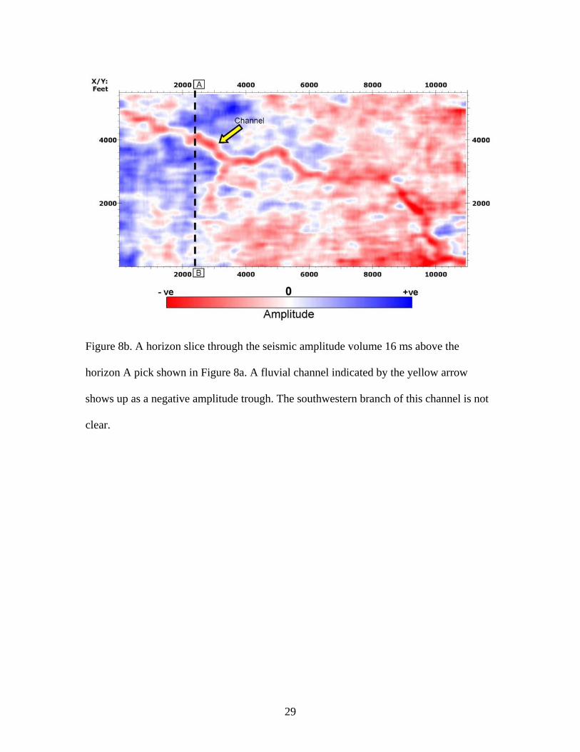
A horizon slice from the Stratton 3D seismic data volume is shown in Figure 8b.
A channel indicated in red appears to have branches in the middle towards south. From
an interpreter's point of view knowing the extension of the possible channel is important
information for reservoir characterization. A 32 Hz frequency slice for the same horizon
slice presented in Figure 9 shows what could be detail of a fluvial channel system. We
observe a pattern similar to that of a complex meandering channel system in the
southwestern part. Also note that the apparent internal heterogeneity of the main fluvial
channel system enhanced by spectral decomposition. The relatively low spectral
amplitude of the channel is indicative of a lithology change (possibly brine filled sand).
14
CONCLUSIONS
A conventional method of computing a time-frequency spectrum, or spectrogram,
using the STFT, requires a pre-defined time window and therefore, has fixed time-
frequency resolution. However, to analyze a non-stationary signal where frequency
changes with time, we require a time varying window. The CWT utilizes the dilation and
compression of wavelets and provides a time-scale spectrum instead of a time-frequency
spectrum. Converting a scalogram into a time-frequency spectrum using the center
frequency of a scale gives an erroneous attenuation in the spectrum. The TFCWT
overcomes this problem and gives a more robust technique of time-frequency
localization. Since TFCWT is fundamentally derived from the continuous wavelet
transform, the dilation and compression of wavelets effectively provides the optimal
window length depending upon the frequency content of the signal. Thus, it eliminates
the subjective choice of a window length and provides an optimal time-frequency
spectrum without any erroneous attenuation effect for a non-stationary signal. It has high
frequency resolution at low frequencies and high time resolution at high frequencies,
whereas the spectrogram has fixed time-frequency resolution throughout. Thus, in non-
stationary seismic data analysis the TFCWT has a natural advantage over the STFT and
the typical CWT spectrum. Though STFT allows one to analyze an entire stratigraphic
interval, this method is focused on the spectral attributes of horizons rather than intervals.
The STFT may be more efficient for estimating the spectral characteristics of long
intervals as compared to the support of the CWT. However, the TFCWT can be summed
over time to resolve the spectrum of any desired interval. The field examples on single

15
frequency sections and maps from the TFCWT presented in this work suggest that such
analysis can potentially be utilized as direct hydrocarbon indicators and for improved
stratigraphic visualization.
ACKNOWLEDGEMENTS
The authors acknowledge the Conoco research scientists for their valuable input.
We would also like to thank Conoco (now ConocoPhillips) for providing a field data set
and logistical support for this research. We particularly thank Dr. Dale Cox of Conoco for
many useful discussions and for his help in the practical implementation in SeismicUnix
(SU). We are grateful to the Shell Crustal Imaging Facility at the University of Oklahoma
for the software support. We thank Dr. Kurt Marfurt, the associate editor of Geophysics,
and two reviewers for their valuable comments and suggestions.
16
REFERENCES
Abry, P., Goncalves, P., and Flandrin, P., 1993, Wavelet-based spectral analysis of 1/f
processes: IEEE Internat. Conf. Acoustic, Speech and Signal Processing, 3, 237-240.
Castagna, J. P., Sun, S., and Seigfried, R. W., 2003, Instantaneous spectral analysis:
Detection of low-frequency shadows associated with hydrocarbons: The Leading Edge,
22, 120-127.
Cohen, L., 1995, Time-frequency analysis: Prentice Hall.
Daubechies, I., 1992, Ten Lectures on wavelets: SIAM Publ.
Dilay, A. and Eastwood, J., 1995, Spectral analysis applied to seismic monitoring of
thermal recovery: The Leading Edge, 14, 1117-1122.
Ebrom, D., 2004, The low frequency gas shadows in seismic sections: The Leading Edge,
23, 772.
Hardy, H. H., Richard, A. B.,and Gaston, J. D., 2003, Frequency estimates of seismic
traces: Geophysics, 68, 370--380.

17
Jones, D. L. and Baraniuk, R. G., 1995, An adaptive optimal-kernel time-frequency
representation: IEEE transactions on signal processing, 43, 2361-2371.
Mallat, S., 1999, A wavelet tour of signal processing, 2nd ed.: Academic Press.
Mallat, S., and Zhang, Z., 1993, Matching pursuits with time-frequency dictionaries:
IEEE transactions on signal processing, 41, 3397-3415.
Marfurt, K. J., and Kirlin, R. L., 2001, Narrow-band spectral analysis and thin-bed
tuning: Geophysics, 66, 1274-1283.
Mitchell, J. T., Derzhi, N., and Lickman, E., 1997, Low frequency shadows: The rule, or
the exception?, 67th Ann.Internat. Mtg. Soc. Expl. Geophys., 685-686.
Partyka, G., Gridley, J., and Lopez, J., 1999, Interpretational applications of spectral
decomposition in reservoir characterization: The Leading Edge, 18, 353-360.
Peyton, L., Bottjer, R., and Partyka, G., 1998, Interpretation of incised valleys using new
3-D seismic techniques: A case history using spectral decomposition and coherency: The
Leading Edge, 17, 1294-1298.
Rioul, O. and Vetterli, M., 1991, Wavelets and signal processing: IEEE Signal Processing
Magazine, Oct, 14-38.
18
Sinha, S., 2002, Time-frequency localization with wavelet transform and its application
in seismic data analysis: Master's thesis, Univ. of Oklahoma.
Sun, S., Castagna, J. P., and Seigfried, R. W., 2002, Examples of wavelet transform time-
frequency analysis in direct hydrocarbon detection: 72nd Ann. Internat. Mtg. Soc. Expl.
Geophys., 457- 460.
Torrence, C., and Compo, G., P., 1998, A practical guide to wavelet analysis: Bulletin of
the American Meteorological Society, 79, 61-78.
19
LIST OF FIGURES
Figure 1. A chirp signal consisting of two known hyperbolic sweep frequencies with
constant amplitude for each frequency.
Figure 2. A spectrogram of the chirp signal using a 400 ms window length. Notice that
the lower frequencies are well resolved but the higher frequencies are not resolved.
Figure 3. A typical CWT spectrum obtained for the chirp signal shown in Figure 1. It is
converted from the scalogram, described by equation (4), using the center frequencies of
scales.
Figure 4. TFCWT spectrum, described by equation 11, obtained for the chirp signal
shown in Figure 1 using a complex Morlet wavelet.
Figure 5. A seismic section from Nigeria data set. Bright amplitudes indicated by yellow
arrows adjacent to the faults (green arrows) in this seismic section are known
hydrocarbon zones.
Figure 6. 20 Hz seismic section of obtained using TFCWT processing of the seismic data
shown in Figure 5. High amplitude low frequency anomalies shown in red are at the
hydrocarbon zones (yellow arrows).
20
Figure 7. 33 Hz seismic section of Figure 5 obtained using TFCWT processing. In this
section frequency anomalies associated with frequency shadows are absent (yellow
arrows). The anomaly present (blue arrow) in this section is due to local tuning effects
and doesn't disappear at higher frequencies.
Figure 8a. A vertical seismic section through the Stratton 3D data set corresponding to
line AB shown in Figure 8b. A channel indicated by yellow arrow corresponds to the
channel shown in Figure 8b.
Figure 8b. A horizon slice through the seismic amplitude volume 16 ms above the
horizon A pick shown in Figure 8a. A fluvial channel indicated by the yellow arrow
shows up as a negative amplitude trough. The southwestern branch of this channel is not
clear.
Figure 9. A horizon slice at 32 Hz through the TFCWT volume corresponding to the
seismic amplitude map shown in Figure 8b. Note the channel extension (blue arrows) and
internal heterogeneity of the fluvial channel system.

21
Figure 1. A chirp signal consisting of two known hyperbolic sweep frequencies with
constant amplitude for each frequency.
22
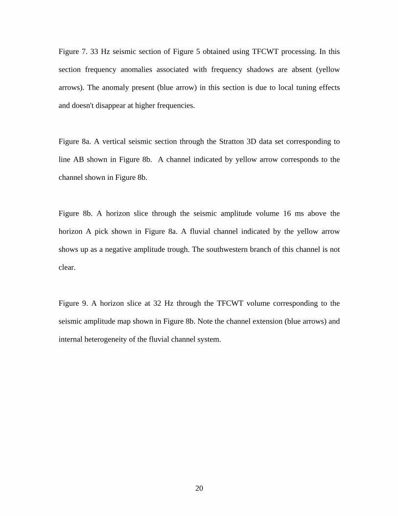
Figure 2. A spectrogram of the chirp signal using a 400 ms window length. Notice that
the lower frequencies are well resolved but the higher frequencies are not resolved.
23
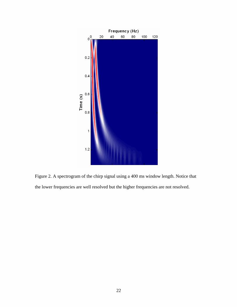
Figure 3. A typical CWT spectrum obtained for the chirp signal shown in Figure 1. It is
converted from the scalogram, described by equation (4), using the center frequencies of
scales.

24
Figure 4. TFCWT spectrum, described by equation 11, obtained for the chirp signal
shown in Figure 1 using a complex Morlet wavelet.
25
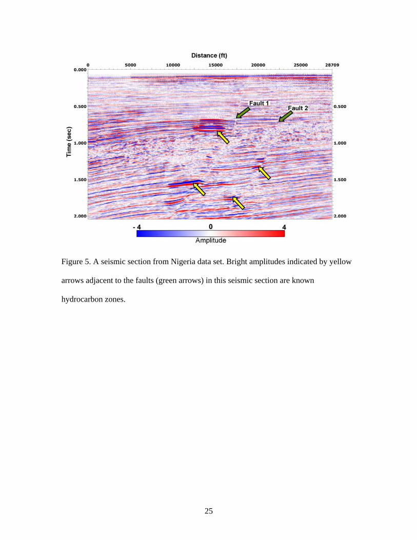
Figure 5. A seismic section from Nigeria data set. Bright amplitudes indicated by yellow
arrows adjacent to the faults (green arrows) in this seismic section are known
hydrocarbon zones.

26
Figure 6. 20 Hz seismic section obtained using TFCWT processing of the seismic data
shown in Figure 5. High amplitude low frequency anomalies shown in red are at the
hydrocarbon zones (yellow arrows).
27
Figure 7. 33 Hz seismic section of Figure 5 obtained using TFCWT processing. In this
section frequency anomalies associated with frequency shadows are absent (yellow
arrows). The anomaly present (blue arrow) in this section is probably due to local tuning
effects and doesn’t disappear at higher frequencies.

28
Figure 8a. A vertical seismic section through the Stratton 3D data set corresponding to
line AB shown in Figure 8b. A channel indicated by yellow arrow corresponds to the
channel shown in Figure 8b.
29
Figure 8b. A horizon slice through the seismic amplitude volume 16 ms above the
horizon A pick shown in Figure 8a. A fluvial channel indicated by the yellow arrow
shows up as a negative amplitude trough. The southwestern branch of this channel is not
clear.

30
Figure 9. A horizon slice at 32 Hz through the TFCWT volume corresponding to the
seismic amplitude map shown in Figure 8b. Note the channel extension (blue arrows) and
internal heterogeneity of the fluvial channel system.