Spectral characteristics of salt-affected soils: A ... · Spectral characteristics of salt-affected soils: A laboratory experiment 58 a b Figure 3.1: a) Kubiena boxes including sponges

Chapter 3

Spectral characteristics of salt-affected soils: A laboratory experiment

Abstract This study focuses on the use of laboratory spectroscopy to recognize the presence and abundance of salts in soils. To create soil samples with large variations in soil salinity, six different saline solutions in various densities were prepared (containing either MgCl2, NaCl, KCl, K2SO4, MgSO4 or Na2SO4). The saline solutions were used to sub-irrigate three sets of soil samples with silty clay loam (nobs = 65), sandy loam (nobs = 41) and sand textures (nobs = 41). After sub-irrigation, soil spectra and soil salinity were measured for each of the 147 samples. Statistical techniques were used to detect and characterise diagnostic absorption bands and to develop predictive regression models between spectral signature and soil salinity levels. Spectral analyses revealed that salt-affected soil samples do not exhibit all of the diagnostic absorption features that were found in the spectra of salt minerals used to treat them. It also showed that the number and clearness of diagnostic

This chapter is based on:

Farifteh, J., van der Meer, F., van der Meijde, M., Atzberger, C. (2006). Spectral characteristics of salt-affected soils: A laboratory experiment. Under review, Geoderma.


54

bands reduces as the salt concentration in the samples decreases. Even if salts were present in high concentrations (EC ≥ 8 dS/m), two commercially available software packages (PimaView and TSG algorithm) were unable to correctly recognize presence of different salts. To quantify salt-abundances across soil types, none of the investigated regression models proved optimal for all salts. In general, predictive models using continuum-removed absorption features gave higher accuracies compared to models using either spectral reflectances at selected wavelengths or models based on overall albedo. Amongst the investigated salts, MgCl2 and MgSO4 were estimated with the highest accuracies (cross-validated R2CV ≥ 0.80 and PRMSECV < 40%). For NaCl, estimation of soil salinity gave an accuracy (R2CV = 0.65 with PRMSECV = 50.3%). Only weak relations could be established to quantify KCl and Na2SO4. Given the high PRMSECV values for these two salts (67.2% and 60.6%, respectively), application of these models must be considered very limited. No useful relation could be established between K2SO4 and the investigated spectral features. The results highlight the limitations of remote sensing for mapping soil salinity. With regard to up-scaling from experiment data to field and eventually to air-borne and space-borne sensors, a number of constraints have to be considered. The main limitation is that most diagnostic spectral features occur close to the water absorption bands around 1400 and 1900 nm and are very small and not diagnostic. Hence, their detection would require a very high spectral resolution, continuous spectral sampling and high signal-to-noise ratio. The recognition of presence and abundance of salts in soils is further complicated by the fact that in natural conditions, soil water and roughness effects, organic matter content, soil mineralogy and BRDF (Bidirectional reflectance distribution function) effects are superimposed on the measured signal. This illustrates the complexity of the implementation of laboratory findings in the analysis of air- and space-borne data where the crucial spectral information is not completely available and/or influenced by other soil constituents.

3.1 Introduction Identification of salt-affected areas is essential for sustainable agricultural management, especially in (semi-) arid environments. Salt-affected soils contain various proportions of cations (Na+, Mg++, K+, and Ca++) and anions (Cl-, SO4- -, CO3- - and HCO3-) that lead to different degrees of salinity. The main source of salt constituents are the primary minerals found in soils and exposed rocks, which appear in the form of a (1) salt crust as a result of evaporation, (2) deposit as a result of precipitation, or (3) solution as a result of dissolving in water in a soil profile (FAO, 1988; Richards, 1954). The minerals mainly responsible for soil

Chapter 3

55

salinity are found within four chemical groups namely carbonates, halides, sulphates, and borates. The mineral groups and their characteristics are extensively discussed by Klein and Hurlbut (1999). Soil salinity is generally measured by soil electrical conductivity (EC) with values ranging between 2 to more than 32 dS/m (Richards, 1954). Remote sensing has been widely used to identify and map saline areas at various scales (e.g., Farifteh, et al., 2006a; Dehaan and Taylor, 2003; Metternicht and Zinck, 2003; Ben-Dor et al., 2002, Evans and Caccetta, 2000; Dwivedi and Sreenivas, 1998; De Jong, 1992; Everitt et al., 1988; Sharma and Bhargava, 1988). Application of broadband remote sensing (e.g. Landsat, SPOT, Aster) in salinity studies is restricted due to the limitations in spatial and spectral resolution and sampling bandwidth that masks detailed spectral signatures (Cloutis, 1996). Three major problems interfere in the detection of salt-affected soils by means of remote sensing: (1) the process goes often undetected, especially when salt minerals have not (yet) severely affected the soils, (2) the physical boundaries separating saline areas of different degrees are fuzzy, and (3) the process of salinization occurs not only at the soil surface but also in the soil profile, which can not be detected by optical sensors. Moreover, in nature, salt minerals are rarely pure, since trace elements are often trapped in crystal lattices during crystallization. This affects the reflectance properties of minerals (Hunt and Salisbury, 1970, 1971) and thus hampers the use of already established experimental models. To map saline soils, different direct and indirect methods have been developed. Besides detecting altered soil optical properties, salt-induced roughness changes and/or modified plant growth pattern can be detected (Ben-Dor 2002; Dehaan and Tayor, 2002; Szilagyi and Baumgardner, 1991; Baumgardner, et al., 1985; Stoner and Baumgardner, 1981). For the analysis of altered soil optical properties, various analytical techniques have been developed. Methods encompass monovariate regressions to multivariate approaches. Recently, partial least squares regression (PLSR) has been extensively used for quantitative analysis of reflectance spectra (Yang et al., 2003; Udelhoven et al., 2003; Wold et al., 2001; Anderson and Bro, 2000; Haaland and Thomas, 1988a, b). Despite all efforts, differentiation between saline areas of different degrees and automatic salt identification are still not sufficiently researched. Technological advances such as (airborne) imaging spectrometry offer considerable potential as the instruments provide high spatial resolution data in a large number of narrow contiguous spectral bands in the VNIR-SWIR region (400 to 2500 nm). As salt minerals have characteristic features occurring in the VNIR-SWIR region, they can be distinguished from one another (Drake, 1995; Crowley, 1991a, b; Gaffey, 1987; Hunt et. al., 1971, 1972).


56

Success in discrimination of saline areas of different degrees can be increased if the spectral characteristics of salt-affected soils and the underlying factors are examined. In this regard, more attention should be given to the analysis of reflectance spectra obtained from soils containing various amount of salts. Through carefully designed laboratory experiments, the contribution of the spectral information derived from the salt minerals in identification of minerals and discrimination of saline areas can be examined. At the same time, the strength of the relationship between amount of salts in soils (electrical conductivity) and their influence on soil spectral characteristics can be analysed in more detail. Consequently, the main aim of this chapter is to provide insight spectral information that leads to a better understanding of spectral behaviour of salt-affected soils and to define a guideline for development of spectrometric techniques with capabilities of recognizing the presence and abundance of salts in soils. To study the relationship between salt concentration in soil samples and its spectral response, a laboratory experiment was designed involving soils with three textures and six salt minerals. The artificially induced soil salinity covered the whole range from non-saline (ECe < 2 dS/m) to extremely saline soils (ECe > 16 dS/m). For predicting salinity levels focus was on monovariate linear regression approaches between EC and spectral features. For salt identification in the soil reflectance spectra, two commercially available software packages (PimaView and TSG algorithm) were used and evaluated.

3.2 Materials and methods

3.2.1 Laboratory experiment design Ideally, it is desired to obtain direct and simultaneous measurements of soil properties, including reflectance, as salinization process progress under natural conditions. To obtain such ideal set of data, essentially requires lysimeter1 facilities, which allow study of soil profiles under various conditions as salinity levels progress due to changing depths of saline water table. However, for practical reasons, a simpler laboratory experiment was designed to control salt accumulation in soil samples. In such a controlled experimental set up, salt concentration in soil samples were varied by simulation of ground water rise and of evaporation processes while soil constituents were kept almost constant in the short period of the experiment. This means any change in soil reflectance

1 The lysimeter is much like a pot that sits in the ground and can accommodate soil, plants, air and water resources. It was developed by Bill Pruitt, and has been used in hundreds of experiments to study e.g., the water and material movement in soil profile, the effects of different soil surface formations and plant covers on the water regime of the soil.

Chapter 3

57

spectra is mainly due to variations in salt content of the soil samples because the other soil properties remain almost the same. Quality assurance and control were formulated according to the published literature concerning guidelines of field and laboratory methods. The fieldwork activities and data collection and their relevance are described separately (see fieldwork actives and materials). The quality control of the experiment activities can be present in steps of samples preparation and measurements. The preparation of the solution was guided by the published methods namely Handbook of chemistry and physics (Lide, 1993). The preparation of the soil samples was guided by soil survey laboratory methods (Burt, 2004; Van Reeuwijk, 1993). The spectral measurements followed procedures found in Hunt and Salisbury (1970 and 1971), Csillag (1993), Crowley (1991a, b), Congalton and Green (1999), NASA (2001) and USGS websites. The ASD user manual (Hatchell, 1999) was consulted for calibration of the spectrometer and the spectral data collection.

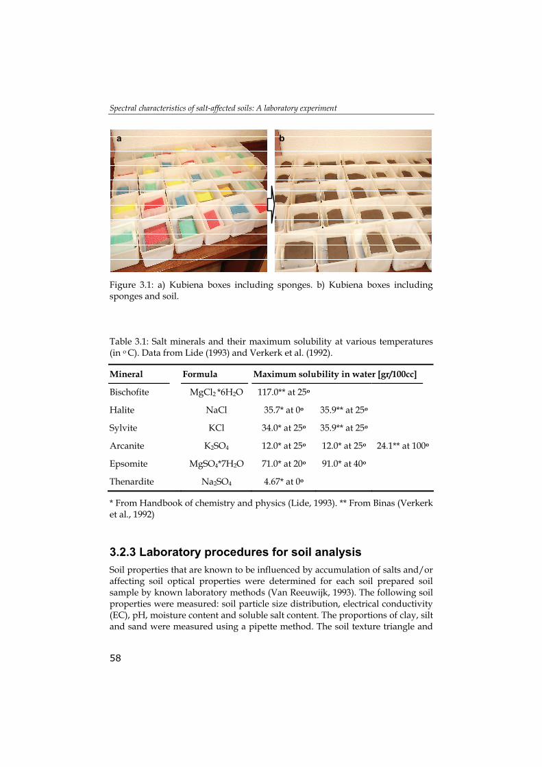
3.2.2 Sample preparation Soil material was air-dried, crushed and passed through a 2 mm sieve (Van Reeuwijk, 1993). The soil samples were, according to texture, divided in three sets. In total, 147 top-open Kubiena boxes were prepared in three sets (65, 41 and 41) each representing a soil texture. The Kubiena boxes in each set were filled with about 50 to 60 grams of soil after a sponge was placed at the bottom of each box (Figure 3.1). The samples were placed in bigger plastic boxes in such a way that added salt solution could move up to the soil through the sponge (simulating groundwater level change). The aqueous salt solutions were prepared in 100 cc of distilled water using standard methods applied in laboratories (Max et al., 2001, Lide, 1993). The technical-grade salts used to prepare the solution are listed in Table 3.1. All salts were purchased as pure (99 or 98 %) from Merck Bv. (http://www.merck.nl). The soil samples were sub-irrigated with saline water and left to dry at room temperature (simulating evaporation process). One sample of each set was treated with distilled water. Different levels of soil salinity were artificially created in this way.


58

a b

Figure 3.1: a) Kubiena boxes including sponges. b) Kubiena boxes including sponges and soil. Table 3.1: Salt minerals and their maximum solubility at various temperatures (in o C). Data from Lide (1993) and Verkerk et al. (1992).

Mineral Formula Maximum solubility in water [gr/100cc]

Bischofite MgCl2 *6H2O 117.0** at 25o

Halite NaCl 35.7* at 0o 35.9** at 25o

Sylvite KCl 34.0* at 25o 35.9** at 25o

Arcanite K2SO4 12.0* at 25o 12.0* at 25o 24.1** at 100o

Epsomite MgSO4*7H2O 71.0* at 20o 91.0* at 40o

Thenardite Na2SO4 4.67* at 0o

* From Handbook of chemistry and physics (Lide, 1993). ** From Binas (Verkerk et al., 1992)

3.2.3 Laboratory procedures for soil analysis Soil properties that are known to be influenced by accumulation of salts and/or affecting soil optical properties were determined for each soil prepared soil sample by known laboratory methods (Van Reeuwijk, 1993). The following soil properties were measured: soil particle size distribution, electrical conductivity (EC), pH, moisture content and soluble salt content. The proportions of clay, silt and sand were measured using a pipette method. The soil texture triangle and

Chapter 3

59

distribution percentages measurements were used to define the soil texture of the samples (Table 3.2). The EC of the samples were determined from soil water extract (1:2 by weight) using air-dry soil and distilled water. The amount of salt cations present in each sample was measured using the ICP-AES (liberty series II Inductively Coupled Plasma Atomic Emission Spectrometer).

3.2.4 Laboratory procedures for spectral data acquisition A portable ASD FieldSpec FR spectrometer (manufactured by Analytical Spectral Devices, Inc.) was employed for the reflectance measurements. The instrument covers the visible to short-wave infrared wavelength range (350 to 2500 nm) using three separate detectors: the VNIR (350 – 1050 nm), the SWIR1 (1000-1800 nm), and the SWIR2 spectrometer (1800 -2500 nm). The spectrometer has a sampling interval of 1.4 nm for the region 350 - 1000 nm and 2 nm for the region 1000 - 2500 nm with a spectral resolution of 3 and 10 nm, respectively (Hatchell, 1999). Reflectance measurements were acquired in a laboratory setting using a 25° foreoptic. A light source (Lowel Light Pro, with JCV 14.5V-50WC halogen lamp) illuminated the sample surface with a 45o zenith angle from a distance of 20 cm. Spectral measurements were taken from nadir at 3 cm height above the sample. Integration time was set to 1 sec. Reflectance was calibrated against a white panel of known reflectance (Spectralon Diffuse Reflectance Panel). All spectral measurements were made in a completely dark room to avoid contamination by stray light.

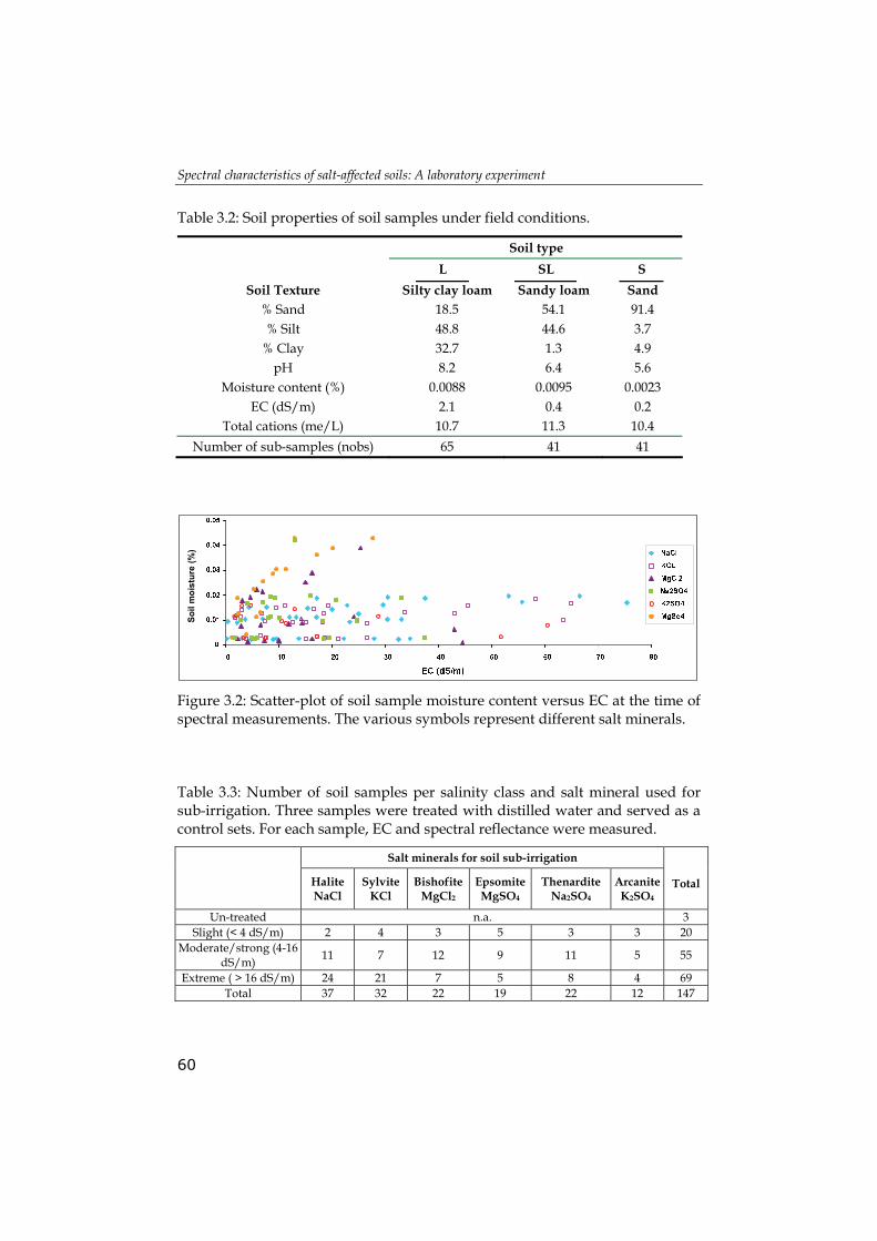
3.2.5 Laboratory measurements The soil samples used in this study were collected from field area in northeast Hungary (silty clay loam soil) and from Texel island in the northwest of The Netherlands (sandy loam and sand).The properties of these soil samples under field conditions are given in Table 3.2. Once the treated samples were dried, their properties were measured. The experimental set-up ensured that soil moisture contents remained low, thus minimizing the effect of soil moisture on the measured spectra. Soil moisture content never exceeded 0.05 %, with more than ¾ of samples having moisture contents of less than 0.02 percent (Figure 3.2). The number of samples per salinity class is shown in Table 3.3 for each of the six salt minerals. Sample numbers varied between 12 (arcanite) and 37 (halite).


60

Table 3.2: Soil properties of soil samples under field conditions.

Soil type L SL S

Soil Texture Silty clay loam Sandy loam Sand % Sand 18.5 54.1 91.4 % Silt 48.8 44.6 3.7

% Clay 32.7 1.3 4.9 pH 8.2 6.4 5.6

Moisture content (%) 0.0088 0.0095 0.0023 EC (dS/m) 2.1 0.4 0.2

Total cations (me/L) 10.7 11.3 10.4 Number of sub-samples (nobs) 65 41 41

Soil

moi

stur

e (%

)

Figure 3.2: Scatter-plot of soil sample moisture content versus EC at the time of spectral measurements. The various symbols represent different salt minerals. Table 3.3: Number of soil samples per salinity class and salt mineral used for sub-irrigation. Three samples were treated with distilled water and served as a control sets. For each sample, EC and spectral reflectance were measured.

Salt minerals for soil sub-irrigation Halite

NaCl Sylvite

KCl Bishofite

MgCl2 EpsomiteMgSO4

Thenardite Na2SO4

Arcanite K2SO4

Total

Un-treated n.a. 3 Slight (< 4 dS/m) 2 4 3 5 3 3 20

Moderate/strong (4-16 dS/m) 11 7 12 9 11 5 55

Extreme ( > 16 dS/m) 24 21 7 5 8 4 69 Total 37 32 22 19 22 12 147

Chapter 3

61

In total, 147 laboratory derived spectra were collected from the saline and air dried soil samples. Reflectance spectra of the six salt minerals (will be discussed later) that were used for sub-irrigating soil samples were also measured. In addition, the spectra of the aqueous solutions of the technical-grade salts (Table 3.1) were measured almost at the limit of their solubility range. The salts in the solution are completely ionized and the ions by themselves do not exhibit absorptions features in the range of 400 - 2500 nm (Figure 3.3). However, the salts solvated water have distinctive spectra which are slightly different from that of pure water and can be analyzed using various techniques (Max and Chapados 2001; Max et al., 2001). Nevertheless, such detailed differences in spectra of salt aqueous solutions do not have a significant impact on remote sensing application of salt-affected soils.

Ref

lect

ance

(Sta

cked

)

Figure 3.3: The spectra of pure water and salt solutions at maximum concentration. The white reference panel was placed under the solution to enhance the measured spectra. The spectra presented in this figure are offset vertically for viewing purpose. To further reduce noise present in the soil spectra, a (polynomial) Savitzky-Golay filter (Savitzky and Golay, 1964) was applied to the measured spectra (order of 2 and frame size of 51 nm). The salt induced variability in soil reflectance is depicted in Figure 3.4 for each soil type separately. The graph shows the spectral signature of the soil treated with distilled water (solid line), as well as the 5% and 95% percentiles per wavelength (dashed lines). For later analysis, only the spectral range between 1000 and 2400 nm has been considered.


62

Ref

lect

ance

Ref

lect

ance

Ref

lect

ance

Figure 3.4: Soil reflectance variability (5% and 95%-percentiles) resulting from sub-irrigation of three soils with saline solutions of various densities (dashed lines). The solid lines correspond to the soils treated with distilled water. All soil spectra were measured in air-dried conditions.

3.2.6 Spectral analysis techniques To analyse and exploit relationships between soil salinity and soil optical properties, linear relations between EC and spectral characteristics were assumed. Two categories of spectral characteristics were analyzed: (1) soil reflectances and (2) absorption features. The measured soil reflectances were either analyzed as a function of wavelength (yielding spectral correlograms in steps of 50 nm) or were spectrally integrated into overall albedo values before analysis. In both cases, analysis was restricted to the wavelength range between 1000 and 2400 nm. As regards the absorption features, characteristics such as depth, depth position (λd) and area of the absorption feature were considered (van der Meer, 2000b; Kruse, 1995). These characteristics were calculated from continuum-removed spectra to enhance absorption features in the recorded soil reflectance spectra. Clark and Roush (1984) were the first to suggest

Chapter 3

63

continuum–removal (CR) analysis to isolate individual absorption features of interest. The continuum is a convex “hull” of straight-line segments fitted over the top of a spectrum that connect local spectral maxima and represents the “background” absorption onto which other absorption features are superimposed (Huang et al., 2004). The continuum is removed by dividing the reflectance value for each point in the absorption feature by the reflectance level of the convex hull at the corresponding wavelength. The local shoulder positions were determined through visual analysis and fixed independent of soil type. They are indicated by circles in the right hand side of Figure 3.5. To assess the validity and accuracy of the various regression models, the cross-validation procedure was used (Duckworth, 1998). In this approach (also called leave-one-out method), n different regression equations are calculated from n-1 samples (n being the sample number). Each time a regression variant is calculated, the calibration model is used to predict the observation that was left out. As the predicted samples are not the same as the samples used to establish the model, the cross-validated root-mean-square error (RMSECV) and coefficient of determination (R2CV) are good indicators of the accuracy of the model in predicting unknown samples. To make the effects of different salts more comparable, differences in average salinity levels were corrected by calculating the cross-validated percentage root-mean-square error (PRMSECV). Using standard statistical software (SPSS), statistics were tested for significance at the 0.01 level. Two commercially available mineral identification algorithms were used to identify salt minerals from the recorded soil spectra (PimaView user manual, 1999; TSG user manual, 2005). The algorithms are based on statistical methods identifying an unknown mineral from a reference library. The PimaView algorithm finds the mixture percentage of that mineral in relation to other minerals identified (PimaView user manual, 1999). The TSG algorithm calculates similarities between mineral spectral and soil samples spectra in 3 spectral regions (1304-1400, 1600-1850 and 2100-2496 nm), thus excluding the water absorption bands. The matching value is scaled between 0 and 1 and is a measure of the “goodness of fit” with 1 being a perfect match and 0 indicating no similarity between reference (i.e. mineral) and sample spectra.

3.3. Results and discussion

3.3.1 Spectral features of salt minerals The reflectance spectra collected from pure salt minerals are shown in Figure 3.5. The absorption features identified in the spectra of these minerals corroborate well with other published results (Drake, 1995; Crowley, 1991a;


64

Gaffey, 1987). Only occasionally, the positions of the absorption features are slightly different probably related to variations in mineral purity, grain size, shape and structural order (Drake, 1995). The VNIR-SWIR absorption features seen in most of these mineral spectra are mainly associated with internal vibration modes of anion groups such as HOH, -OH, and SO4-2 or of water, molecules which are trapped, adsorbed or associated in some way with the crystal structure (Crowley, 1991a; Hunt and Salisbury, 1970). For example, the absorption features seen near 1000, 1200, 1400 and 1900 nm in the spectra of hydrated minerals such as epsomite and bischofite are related to vibrations of these anion groups. They show relatively broad absorption features, due to the overlapping bands of water molecules while less hydrated species show narrower absorption bands (Crowley, 1991a). The broad absorption bands near 1400 and 1900 nm in spectra of halite and thenardite are related to the presence of fluid inclusions and/or absorbed water (Crowley, 1991a).

3.2.2 Salt-induced absorption features in CR-spectra Continuum-removed (CR) reflectance spectra of soils treated with six different salt minerals are displayed in Figure 3.6 with different colours representing three levels of salinity. The soil samples in Figure 3.6 (a) and (b) contain halite (NaCl) and sylvite (KCl) as the dominant evaporite minerals. In arid and semi-arid regions, these minerals are amongst the most widespread. The salts mainly occur in form of crystals or efflorescence as a result of evaporation of trapped bodies of salt water. The continuum-removed soil spectra show consistent absorption features at approximately 1440 and 1933 nm, which are also present in the pure mineral spectra of halite and sylvite (Figure 3.5). The features noted at 1440 nm in the spectra of the minerals appear at around 1420 nm in the soil spectra. For both minerals, there is a slight trend of increasing absorption depths with increasing salt concentration. The band at approximately 2204 nm becomes less developed as samples become more saline. The degradation of this band may occur as a result of loss of crystallinity in the clay minerals. This result coincides with findings of Dehaan and Taylor (2002).

Chapter 3

65

1000

1500

2000

0.6

0.7

0.8

0.91

Hal

ite (N

aCl)

1000

1500

2000

Sylv

ite (K

Cl)

1000

1500

2000

Bis

chof

ite (M

gCl 2*

6 H

2O)

1000

1500

2000

00.2

0.4

0.6

0.81

Wav

elen

gth

Then

ardi

te (N

a 2SO

4)

1000

1500

2000

0.9

0.92

0.94

0.96

0.981

Arc

anite

(K2S

O4)

1000

1500

2000

0.9

0.92

0.94

0.96

0.981

Epso

mite

(MgS

O4 *7

H2O

)

0.6

0.7

0.8

0.91

00.2

0.4

0.6

0.81

Wav

elen

gth

Wav

elen

gth

1000

1500

2000

2500

00.1

0.2

0.30.4

0.5

0.6

0.7

0.8

0.91

Wav

elen

gth

Hal

ite

Sylv

ite

Bis

chof

ite

Arc

anite

Then

ardi

te

Epso

mite

Figu

re 3

.5: L

abor

ator

y sp

ectr

a (1

000-

2500

nm

) of s

ix s

alt m

iner

als

used

in th

is s

tudy

: (le

ft) r

efle

ctan

ce s

pect

ra; (

righ

t) ab

sorp

tion

feat

ures

en

hanc

ed t

hrou

gh c

ontin

uum

rem

oval

(so

lid l

ines

) an

d re

flect

ance

spe

ctra

(da

shed

lin

es).

All

mea

sure

men

ts h

ave

been

filt

ered

with

a

Savi

tzky

-Gol

ay (p

olyn

omia

l) sm

ooth

ing

filte

r (p

olyn

omia

l ord

er o

f 2 a

nd fr

ame

size

of 5

1 nm

) bef

ore

disp

lay.

On

the

righ

t han

d si

de, t

he

orig

inal

ref

lect

ance

spe

ctra

(da

shed

lin

es)

are

disp

laye

d to

geth

er w

ith t

he a

ppro

xim

ate

posi

tions

of

the

abso

rptio

n sh

ould

ers

(cir

cles

). O

ccas

iona

lly, t

he re

flect

ance

spe

ctra

had

to b

e of

fset

for b

ette

r dis

play

.


66

The spectra in Figure 3.6c (bischofite) were obtained from soil samples treated with MgCl2 solution. Compared to the bischofite spectra (Figure 3.5), they lack the absorption features at wavelength 1190 and 1824 nm. The shoulder observed at 1556 nm is comparable with the one noted in the spectrum of bischofite. The features at around 1451 and 1952 nm are weaker in the soil spectra and their positions shift as the amount of the salt abundance in the soil decreases. This is due to the fact that soil absorption features around 1400 and 1900 nm broaden as the salt concentration in soil increases.

Halite (NaCl)

CR

refle

ctan

ce

a

0.2

0.4

0.6

0.8

1

b

Sylvite (KCl)

Wavelength

Arcanite (K2SO4)

e

24001200 1400 1600 1800 2000 2200

CR

refle

ctan

ce

0.2

0.4

0.6

0.8

1

Bischofite (MgCl2 *6H2O)

c

CR

refle

ctan

ce

0.2

0.4

0.6

0.8

1

Thenardite (Na2SO4)

d

4<EC<16

EC<4

EC>16

Epsomite (MgSO4 *7H2O)

f

Wavelength

24001200 1400 1600 1800 2000 2200

Figure 3.6: Continuum-removed reflectance spectra of soils treated with different salt minerals. Colours correspond to different levels of salinity: EC< 4 (blue line), 4 < EC < 16 (green line), and EC > 16 (red line). The results are calculated across soil types. The numbers of observations per class are given in Table 3.3. The absorption bands (1410 and 1929 nm) noted in the thenardite spectrum (Na2SO4; Figure 3.5) are also found in saline soils spectra (Figure 3.6d), albeit we observe a slight shift in their positions. The CR-spectra indicate a strong negative correlation between increase of soil EC and changes in absorption bands parameters (depth, width and area).

Chapter 3

67

Absorption features at 1430, 1932 and 2080 nm noted in the spectra of arcanite (K2SO4; Figure 3.5) also appear in the spectra of saline soil samples (Figure 3.6e). However, the soil spectra lack the absorption features at 2279 nm and the band at 2080 nm appears only in the spectrum of moderately to severely saline soils. In general, the positions of the absorption bands in the soil samples are slightly different from arcanite. For this mineral, the absorption features around 1420 and 1930 nm are flattened and slightly reduced in size when the salt concentration increases (Figure 3.6e). However, there is no strong correlation between salt concentration and the clearness of CR absorption features for this salt mineral. The spectra of epsomite (MgSO4) and saline soils samples treated with this mineral are almost identical in the range between approximately 1300 to 2400 nm (Figure 3.5 and Figure 3.6f). All spectra, however, lack the band at 1234 nm. The band at 1631 nm is only exhibited by severely saline soils. All the spectra of severely affected samples rich in epsomite lack the absorption band at around 2204, while slightly to moderately affected samples exhibit the band at this region. The results also indicate that the position of the maximum reflectance shifts toward shorter wavelengths as the salt concentration increases.

3.3.3 Salt-induced reflectance and albedo changes The normalized albedo of saline soil samples is plotted as a function of soil salinity (EC) in Figure 3.7. The normalized albedo is the albedo of a saline sample (Σρλ) divided by the albedo of the same soil treated with distilled water. The graph illustrates that the overall albedo may increase or decrease with salt amount, depending on the salt mineral and soil texture (see also Table 3.5). Results indicate that the abundance of thenardite (Na2SO4) causes much higher soil albedo. The same holds for arcanite (K2SO4). In the latter case, however, the increase in albedo is restricted to the sandy loam and sand samples (Figure 3.7 and Table 3.4). A strong decrease in soil albedo is observed for samples treated with epsomite (MgSO4) and bischofite (MgCl2). In both cases, the decrease in soil albedo with increasing soil salinity can be observed across soil types. The effects of halite (NaCl) and sylvite (KCl) on overall albedo do not reveal a strong and consistent trend in relation to soil EC. The influence of soil texture is clearly visible from samples treated with thenardite (Na2SO4) and epsomite (MgSO4). The effect of both salt minerals on overall albedo increases as soil textures changes from silty clay loam to sandy loam and to sand (Table 3.4). This behaviour can be related to the specific soil surface which decreases from silty clay loam to sand. Variation in soil albedo can also be related to the surface conditions. In general, salts crystals or efflorescence were formed at the surface of the most severely affected soil


68

samples. Samples treated with epsomite, generally, showed a harder surface than e.g., samples treated with halite. However, a detail description of surface conditions can be very long since this experiment used more than 140 samples with salinity level varies between non to severely, which imply a large variety of surface conditions.

0 50 1000.5

1

1.5

2

2.5

EC (dS/m)0 50 100

0.5

1

1.5

2

2.5

EC (dS/m)

Nor

mal

ized

alb

edo

(100

0 -2

400

nm)

Silty clay loam

Na2SO4

MgSO4MgCl2

K2SO4

NaCl

KCl

Sandy loam

Na2SO4

MgCl2MgSO4

K2SO4

KCl

NaCl

0 50 1000.5

1

1.5

2

2.5

EC (dS/m)

Na2SO4

MgSO4MgCl2

K2SO4

KClNaCl

Sand

Figure 3.7: Normalized albedo (1000 – 2400 nm) as a function of soil salinity (EC) for six salts and three different soil types. The normalized albedo is the albedo of a saline sample (Σρλ) divided by the albedo of the same soil treated with distilled water. The different colours represent different salts. The strength of the relations is indicated in Table 3.4. To illustrate the spectral dependence of the relation between soil reflectance and soil salinity, so called correlograms have been calculated across soil types for all salts (Figure 3.8). The correlograms report the coefficient of correlation (r) between soil reflectance and soil salinity as a function of wavelength. They have been calculated from reflectance spectra convoluted with a median filter (size 50 nm) using non-overlapping block processing.

Chapter 3

69

A consistently positive correlation is observed for the samples treated with thenardite (Na2SO4) and arcanite (K2SO4). The results for the samples treated with bischofite (MgCl2) and epsomite (MgSO4) indicate a strong negative correlation, in particular in the spectral region above 1400 nm. Below 1400 nm, the influence of epsomite on soil reflectance is inconsistent, with correlations varying between positive and negative values. The correlograms of the samples treated with halite (NaCl) and sylvite (KCl) indicate no wavelength with a significant relationship between EC and soil reflectance. For these two salts, the coefficient of correlation (r) always remains between ± 0.5 for all wavelengths (Figure 3.8).

1000 1200 1400 1600 1800 2000 2200 2400

0.8

1

Wavelength (nm)

KClMgSO4

MgCl2

NaCl

K2SO4

Na2SO4

0.6

0.4

0.2

0

- 0.2

- 0.4

- 0.6

- 0.8

- 1

Figure 3.8: Coefficient of correlation (r) as a function of wavelength between soil reflectance and soil salinity (EC) across soil types. The different colours indicate six different salts. The circles indicate the positions of maximum (positive or negative) correlation. To reduce calculation time, the correlogram is calculated from reflectance spectra convoluted with a median filter (size 50 nm) using non-overlapping block processing.


70

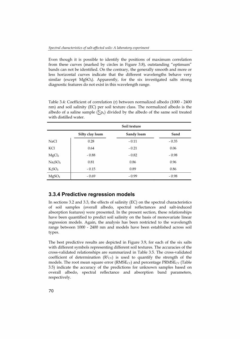
Even though it is possible to identify the positions of maximum correlation from these curves (marked by circles in Figure 3.8), outstanding “optimum” bands can not be identified. On the contrary, the generally smooth and more or less horizontal curves indicate that the different wavelengths behave very similar (except MgSO4). Apparently, for the six investigated salts strong diagnostic features do not exist in this wavelength range.

Table 3.4: Coefficient of correlation (r) between normalized albedo (1000 - 2400 nm) and soil salinity (EC) per soil texture class. The normalized albedo is the albedo of a saline sample (∑ρλ) divided by the albedo of the same soil treated with distilled water.

Soil texture

Silty clay loam Sandy loam Sand

NaCl 0.28 - 0.11 - 0.35

KCl 0.64 - 0.21 0.06

MgCl2 - 0.88 - 0.82 - 0.98

Na2SO4 0.81 0.86 0.96

K2SO4 - 0.15 0.89 0.86

MgSO4 - 0.69 - 0.99 - 0.98

3.3.4 Predictive regression models In sections 3.2 and 3.3, the effects of salinity (EC) on the spectral characteristics of soil samples (overall albedo, spectral reflectances and salt-induced absorption features) were presented. In the present section, these relationships have been quantified to predict soil salinity on the basis of monovariate linear regression models. Again, the analysis has been restricted to the wavelength range between 1000 - 2400 nm and models have been established across soil types. The best predictive results are depicted in Figure 3.9, for each of the six salts with different symbols representing different soil textures. The accuracies of the cross-validated relationships are summarized in Table 3.5. The cross-validated coefficient of determination (R2CV) is used to quantify the strength of the models. The root mean square error (RMSECV) and percentage PRMSECV (Table 3.5) indicate the accuracy of the predictions for unknown samples based on overall albedo, spectral reflectance and absorption band parameters, respectively.

Chapter 3

71

The results suggest that only for five of the six salts, predictive regression models could be established with R2CV ≥ 0.52: NaCl, KCl, MgCl2, Na2SO4 and MgSO4 (Table3.5). No valuable predictive model was found for K2SO4. Amongst the five remaining salts, only for two salts (MgCl2 and MgSO4) the salinity levels could be predicted with RMSECV lower than 6 dS/m (roughly equivalent to PRMSECV lower than 40%). For the remaining three salts (NaCl, KCl and Na2SO4), RMSECV were in the range 7.9 ≤ RMSECV ≤ 16.9 dS/m (PRMSECV between 50.3 and 67.2%). In most cases, predictive models using absorption band features gave better results than models using spectral reflectances or overall albedo (Table 3.5). Visual inspection of Figure 3.9 reveals that the salinity level of sandy soil samples is often slightly overestimated, while the loamy samples have a tendency to be underestimated (e.g. Na2SO4). However, statistical test revealed that the differences related to soil texture are not statistically significant (at the 0.01 level).

3.3.5 Salt identification The mineral identification algorithm (PimaView user manual, 1999) was applied to the 144 (exclude 3 samples representing field conditions) spectra obtained from salt-affected soil samples. The results of the mineral identification are summarised in a confusion matrix (Table 3.6). The results indicate that the accuracy and reliability of mineral identification is very low for all minerals. The calculated overall accuracy of 20.8 % and average reliability and accuracy of 27.1 % and 17.0 %, respectively, indicate low potential for identifying salt types in soils using spectral measurements in the VNIR-SWIR region. The similarity between mineral spectra and the spectra obtained from the saline soil samples was also examined using 'The Spectral Geologist' software (TSG user manual, 2005). The spectral matching technique was used to calculate the spectral similarity between the salt minerals and severely to extremely saline soil samples (EC ≥ 8) treated with the minerals (nobs = 100). A soil sample was said to be correctly identified if the goodness-of-fit value for the correct salt was higher than those of all other minerals. The results (not shown) confirm again the low potential of the VNIR-SWIR to correctly identify the different salt minerals, even for severely to extremely saline samples.


72

Chapter 3

73

0

20

40

60

0 20 40 60 80

0

10

20

30

40

0 10 20 30 40 50

R2 = 0.84

MgCl2 by spectral reflectance (1925 nm)

Silty clay loamSandy loamSand

R2 = 0.8

MgSO4 by area (around 1480 nm)

R2 = 0.52

KCl by depth (around 1430 nm)

Measured EC (dS/m)

R2 = 0.05

K2SO4 by spectral reflectance (2275 nm)

Na2SO4 by spectral reflectance (1825 nm)

R2 = 0.15

0 20 40 60 800

20

40

60

80

Measured EC (dS/m)

0 20 40 60 800

20

40

60

80NaCl by area

(around 1930 nm)

R2 = 0.65

0

20

40

60

0 10 20 30 40 50

0

10

20

30

40

0 10 20 30

Figure 3.9: Measured against estimated EC. All estimations are cross-validated (leave-one-out). For each salt mineral, only the result of the best predictive model is shown. The different symbols represent different soil types: Silty clay loam ( ), Sandy loam ( ) and Sand ( ). The corresponding cross-validated statistics are listed in Table 3.6.


74

Table 3.6: Summarized results of the PimaView mineral identification algorithm applied to spectra obtained from salt-affected soil samples treated with six salt minerals.

Minerals Ha Sy Bi Ep Th Ar Un. Total ACC

Halite (Ha) 2 26 0 1 1 0 7 37 0.05 Sylvite (Sy) 1 24 0 0 0 0 7 32 0.75 Bischofite (Bi) 6 7 0 0 0 0 9 22 0.00 Epsomite (Ep) 2 11 0 3 0 0 3 19 0.16 Thenardite (Th) 5 12 0 0 1 0 4 22 0.05 Arcanite (Ar) 2 10 0 0 0 0 0 12 0.00 Total 18 90 0 4 2 0 30 144 0.21

REL 0.11 0.27 0.00 0.75 0.50 0.00

ACC = Accuracy, REL = Reliability, Un. = Unclassified

3.4 Conclusion The results presented in this chapter provided insight spectral information concerning salt-affected soils. It revealed positive aspects and limitations of remote sensing applications in monitoring and mapping saline areas. The results obtained from this experimental study allow drawing the following conclusions:

The results showed that an increase in soil salinity induces changes in soil reflectance for wavebands higher than 1300 nm, particularly in the water absorption bands (around 1400 and 1900 nm). It also revealed that the relation between salinity level and albedo and/or spectral reflectance may be positive or negative, depending on salt mineral and soil type.

It was found that the observed absorption features at further than 1400

nm were broaden, the position of maximum reflectance were shifted toward shorter wavelengths and overall reflectance were changed proportionally as salts concentration were increased in soil. The continuum-removed (CR) spectra indicate a strong negative correlation between increase of soil EC and changes in absorption bands parameters (depth, width and area).

For all except one salt (K2SO4), statistically significant predictive

regression models could be established. Linear spectral models to predict salinity level (EC) across soil types gave cross-validated root

Chapter 3

75

mean square errors (RMSECV) between 3.7 and 16.9 dS/m (0.51≤R2CV≤0.87). Amongst the investigated spectral variables, those based on continuum-removed absorption features were generally the most accurate. However, the most accurate predictive models were based on spectral reflectances of selected wavelengths previously identified from spectral correlograms. The least accurate were models based on overall albedo.

The results showed that soil samples with large variations in salts did

not exhibit all of the diagnostic absorption features that can be found in the spectra of the dominant salt minerals. It showed that the number and clearness of diagnostic bands reduces as the salt concentration in the samples decreases.

The present study also revealed number of limitations for salt

identification and salinity mapping. The results showed that the absorption bands in the reflectance spectra of pure minerals were less distinctive in saline soil samples, even when salt concentrations were high (EC≥8 dS/m). In some cases, the number and/or position of absorption features varied between pure minerals and salt affected soils. Moreover, in spectra of salt-affected soil, most salt diagnostic absorption features occur close to known water (vapour) absorption bands.

The results suggests that further studies are required to unravel the

influence of soil status (e.g. soil composition, soil roughness, soil water content) on the relation between salinity level and spectral signature. The results also suggest that the quantification of salt-affected soil spectra should largely focus on spectral variations in NIR and SWIR region of soil spectra rather than individual diagnostic absorption signature. At up-scaling phase, quantification of salt-abundances in soil, should mainly focus on using general shape of spectrum rather than absorption bands parameters (depth, area, etc.), since most of the spectral features that are diagnostic of salt minerals or salt-affected soils are masked in an image due to atmospheric effect.

Documents

Spectral characteristics of salt-affected soils: A ... · Spectral characteristics of salt-affected soils: A laboratory experiment 58 a b Figure 3.1: a) Kubiena boxes including sponges