Embed Size (px)
Citation preview
Spectra of Weighted Directed Graphs
A Thesis Submitted
in Partial Fulfillment of the Requirements
for the Degree of
Doctor of Philosophy
by
Debajit Kalita
to the
Department of Mathematics
Indian Institute of Technology Guwahati
Guwahati-781039, India
March, 2012
Declaration
I do hereby declare that the work contained in this thesis entitled “Spectra of
Weighted Directed Graphs’ has done by me, under the supervision of Dr.
Sukanta Pati, Associate Professor, Department of Mathematics, Indian Institute
of Technology Guwahati for the award of the degree of Doctor of Philosophy and
this work has not been submitted elsewhere for a degree.
March, 2012Debajit Kalita
Roll No. 06612303
Department of Mathematics
Indian Institute of Technology Guwahati
i
TH-1064_06612303
Certificate
It is certified that the work contained in this thesis entitled “Spectra of Weighted
Directed Graphs” by Debajit Kalita, a student of Department of Mathematics,
Indian Institute of Technology Guwahati, for the award of the degree of Doctor of
Philosophy has been carried out under my supervision and this work has not been
submitted elsewhere for a degree.
March, 2012Dr. Sukanta Pati
Associate Professor
Department of Mathematics
Indian Institute of Technology Guwahati
TH-1064_06612303

Dedicated
to
My Parents
TH-1064_06612303
Acknowledgements
In the first place I would like to express my gratitude to Dr. Sukanta Pati, for his
supervision, advice, and guidance from the very first day of my research work. His
Socratic questioning, constructive criticism and incredible experience have helped
me to enrich my growth as a researcher in Mathematics. I will be always indebted
to him for his unflinching encouragement and support in various ways.
It is a great pleasure to express my sincere thanks to Prof. R. B. Bapat for his
invaluable suggestions on my research papers and his great influence to my work.
I am deeply indebted to Prof. Meenaxi Bhattacharjee for her encouragements
during the most critical period of my academic career, which exceptionally inspired
me to enrich my basic mathematics skills. Dr. S. N. Bora, Prof. B. K. Sarma,
Prof. K. C. Chowdhury, and Prof. H. K. Saikia are some of the personalities I
would like to acknowledge for giving me the motivation, inspiration and information
required to enter into the research world of mathematics.
The interesting feedback, useful suggestions, support and friendship from Dr.
Anjan Kr. Chakrabarty, Dr. Bikash Bhattacharjya and Biswajit da throughout this
journey, has been invaluable to me on both academic and personal level, for which
I am extremely grateful to them.
I sincerely acknowledge Indian Institute of Technology Guwahati for providing me
with the various facilities necessary to carry out my research. I am most grateful to
CSIR, India for providing me with the financial assistance during the Ph.D process.
I express my special and heartiest thanks to my best friends ever Manoj, Ujwal
and Kuki, who always stand beside me with their support and helping hands in my
difficult times. Besides, I thank all my research scholar friends of the Department of
Mathematics, IIT Guwahati for their love and company during my stay in the IIT
campus.
Finally, I thank my parents, sisters Pranita and Binita, brother Nabajit for their
unequivocal support, unwavering love, quiet patience, and most importantly allowing
me to be as ambitious as I wanted.
March, 2012 Debajit KalitaIIT Guwahati
iv
TH-1064_06612303
Abstract
The study of mixed graph and its Laplacian matrix have gained quite a bit of
interest among the researchers. Mixed graphs are very important for the study of
graph theory as they provide a setup where one can have directed and undirected
edges in the graph. In this thesis we present a more general structure than that
of mixed graphs, namely the weighted directed graphs. We supply appropriate
generalizations of several existing results in the literature for mixed graphs. We
also prove many new combinatorial results relating the Laplacian (resp. adjacency)
matrix and the graph structure. The notion of 3-colored digraphs is introduced here.
This notion naturally generalizes the notion of mixed graphs but is much restricted
in comparison to the weighted directed graph. Our main objective is to study the
spectral properties of the adjacency and the Laplacian matrix of these graphs.
We establish that the Laplacian matrix of weighted directed graphs are not always
singular. A weighted directed graph is said to be singular (resp. non-singular) if its
Laplacian matrix is singular (resp. non-singular). We give several characterizations
of singularity of the weighted directed graphs. Apart from these, we provide some
additional characterization of singularity of the connected 3-colored digraphs. A
combinatorial description of the determinant of the Laplacian matrix of weighted
directed graphs is supplied here.
We prove that the adjacency (resp. Laplacian) spectrum of a 3-colored digraph
can be realized as a subset of the adjacency (resp. Laplacian) spectrum of a suitable
undirected graph. In order to achieve this some graph operations similar to that
in [17] are introduced. Using these graph operations we show that for a connected
3-colored digraph on n vertices, there exists a mixed graph on 2n vertices whose
adjacency and Laplacian eigenvalues are precisely those of the 3-colored digraph
with multiplicities doubled. We also show that for a connected mixed graph G on n
vertices, there is an unweighted undirected graph H on 2n vertices whose adjacency
(resp. Laplacian) spectrum contains the adjacency (resp. Laplacian) spectrum of the
TH-1064_06612303
mixed graph. Moreover, a description of the remaining adjacency (resp. Laplacian)
eigenvalues of H is supplied. We observe that the graph H may be viewed as the
result of a special case of a new graph operation on unweighted undirected graph
introduced here. We show that the adjacency (resp. Laplacian) spectrum of the
graph resulting from such an operation is completely determined by the adjacency
(resp. Laplacian) spectra of some closely related weighted directed graphs.
The Laplacian spectrum of the class of connected 3-colored digraphs containing
exactly one non-singular cycle is studied here. Mainly, we study the smallest Lapla-
cian eigenvalue and the corresponding eigenvectors of such graphs. We show that
the smallest Laplacian eigenvalue of such a graph can be realized as the algebraic
connectivity (second smallest Laplacian eigenvalue) of a suitable undirected graph.
We determine the non-singular unicyclic 3-colored digraph on n vertices, which min-
imize the smallest Laplacian eigenvalue over all such graphs. A class of non-singular
unicyclic 3-colored digraphs maximizing the smallest Laplacian eigenvalue over all
such graphs is also supplied. We give a complete characterization of non-singular
unicyclic 3-colored digraphs that have 1 as the second smallest Laplacian eigenvalue.
A combinatorial description of the coefficients of characteristic polynomial of the
adjacency matrix of 3-colored digraphs is supplied here. We obtain a relationship
between these coefficients and the structural properties of the graph, generalizing
Sachs theorem. A graph G is said to have SR-property if A(G) is non-singular and
λ is an eigenvalue of A(G) of multiplicity k if and only if 1λ
is an eigenvalue of A(G)
with the same multiplicity. Finally, we supply the structure of unicyclic 3-colored
digraphs satisfying SR-property.
vi
TH-1064_06612303
Contents
Abstract v
1 Introduction 1
1.1 Preamble . . . . . . . . . . . . . . . . . . . . . . . . . . . . . . . . . 1
1.2 Organization of the Thesis . . . . . . . . . . . . . . . . . . . . . . . . 5
2 Laplacian singularity of weighted directed graphs 7
2.1 D-similarity and Laplacian singularity . . . . . . . . . . . . . . . . . 7
2.2 Edge singularity of weighted directed graph . . . . . . . . . . . . . . 14
2.3 3-colored digraphs and their singularity . . . . . . . . . . . . . . . . 18
2.4 Determinant of the Laplacian matrix of weighted directed graph . . 22
3 Spectra of 3-colored Digraphs 25
3.1 Mixed Graphs whose spectrum contains the spectrum of a given 3-
colored digraph . . . . . . . . . . . . . . . . . . . . . . . . . . . . . . 26
3.2 Realizability of the spectrum of a mixed graph by an unweighted
undirected graph. . . . . . . . . . . . . . . . . . . . . . . . . . . . . . 30
3.3 Spectrum of an unweighted undirected graph resulting from a more
general graph operation . . . . . . . . . . . . . . . . . . . . . . . . . 36
4 3-colored digraphs with exactly one non-singular cycle 40
4.1 Smallest Laplacian eigenvalue . . . . . . . . . . . . . . . . . . . . . . 40
4.2 First eigenvectors of Gg . . . . . . . . . . . . . . . . . . . . . . . . . 46
4.3 Minimizing the smallest Laplacian eigenvalue over unicyclic 3-colored
digraphs . . . . . . . . . . . . . . . . . . . . . . . . . . . . . . . . . . 53
vii
TH-1064_06612303
Contents
4.4 Maximizing the smallest Laplacian eigenvalue over unicyclic 3-colored
digraphs . . . . . . . . . . . . . . . . . . . . . . . . . . . . . . . . . . 61
4.5 Unicyclic 3-colored digraph with second smallest Laplacian eigenvalue
equal to 1 . . . . . . . . . . . . . . . . . . . . . . . . . . . . . . . . . 62
5 Unicyclic 3-colored digraphs with SR-property 67
5.1 Characteristic polynomial of A(G) . . . . . . . . . . . . . . . . . . . 67
5.2 3-colored digraphs with SR-property . . . . . . . . . . . . . . . . . . 69
5.3 Unicyclic 3-colored digraphs with a blue edge on C . . . . . . . . . . 73
5.4 Unicyclic 3-colored digraph with a green edge on C . . . . . . . . . . 79
Bibliography 81
viii
TH-1064_06612303
Chapter 1
Introduction
1.1 Preamble
The study of graph spectra is an important part of graph theory. It has found its
applications in several subjects like Biology, Geography, Economics, Social Sciences,
computer science, information and communication technologies, see for example [15]
and references there in. Several researchers have studied various spectral properties
of the adjacency and Laplacian matrices of graphs. We refer the reader to the
classical book by Cvetkovic, Doob and Sachs [13] and the survey articles by Merris
[35] and Mohar [38], for more background on these matrices.
All our graphs are simple. All our directed graphs have simple underlying undi-
rected graphs (except in Remark 3.3.2 and Definition 4.1.8). At times we use V (G)
(resp. E(G)) to denote the set of vertices (resp. edges) of a graph G (directed or
undirected). In the absence of any specification V (G) is assumed to be {1, 2, . . . , n}.We write (i, j) ∈ E(G) to mean the existence of the directed edge from the vertex i
to the vertex j. Throughout the thesis i =√−1.
Definition 1.1.1. Let G be a directed graph. With each edge (i, j) in E(G) we
associate a complex number wij of unit absolute value and non-negative imaginary
part. We call it the weight of that edge. We call the directed graph G with such a
weight function w a weighted directed graph.
Definition 1.1.2. Let G be a weighted directed graph. We define the adjacency
matrix A(G) of G as the matrix with ij-th entry
aij =
wij if (i, j) ∈ E(G),wji if (j, i) ∈ E(G),0 otherwise.
1
TH-1064_06612303
Chapter 1 Introduction
Remark 1.1.3. Note that choosing the weights only from the ‘upper half part of
the unit circle’ in Definition 1.1.1 is not really a restriction for the study of adjacency
matrices. For example, if G has an edge (i, j) of weight x + yi, then we may replace
that edge by an edge (j, i) of weight x − yi while the adjacency matrix remains
unchanged.
Let G be a weighted directed graph. In defining subgraph, walk, path, component,
connectedness, matching and degree of a vertex in G we focus only on the underlying
unweighted undirected graph of G. The degree di of a vertex i in a weighted directed
graph G may be viewed as the sum of absolute values of the weights of the edges
incident with the vertex i.
Definition 1.1.4. Let G be a weighted directed graph. We define the Laplacian
matrix L(G) of G as the matrix D(G) − A(G), where D(G) is the diagonal matrix
with di as the i-th diagonal entry.
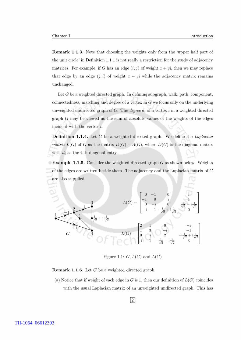
Example 1.1.5. Consider the weighted directed graph G as shown below. Weights
of the edges are written beside them. The adjacency and the Laplacian matrix of G
are also supplied.
b
b
b
b
1
2
3
4
i
1−1
i
1√2
+ i 1√2
G
A(G) =
0 −1 0 i−1 0 i 1
0 −i 0 1√2− i 1√
2
−i 1 1√2
+ i 1√2
0
L(G) =
2 1 0 −i1 3 −i −10 i 2 − 1√
2+ i 1√
2
i −1 − 1√2− i 1√
23
Figure 1.1: G,A(G) and L(G)
Remark 1.1.6. Let G be a weighted directed graph.
(a) Notice that if weight of each edge in G is 1, then our definition of L(G) coincides
with the usual Laplacian matrix of an unweighted undirected graph. This has
2
TH-1064_06612303
Chapter 1 Introduction
motivated us to use D(G)−A(G) rather than D(G) + A(G) for the Laplacian
matrix.
(b) If weights of the edges in G are ±1, then (viewing the edges with weight 1 as
directed and the edges with weight −1 as undirected) our definition of L(G)
coincides with the Laplacian matrix of a mixed graph as defined in [4].
(c) If weight of each edge in G is −1, then our definition of L(G) coincides with the
well studied signless Laplacian matrix (see for example, Cvetkovic, Rowlinson
and Simic [14]) of undirected graph G.
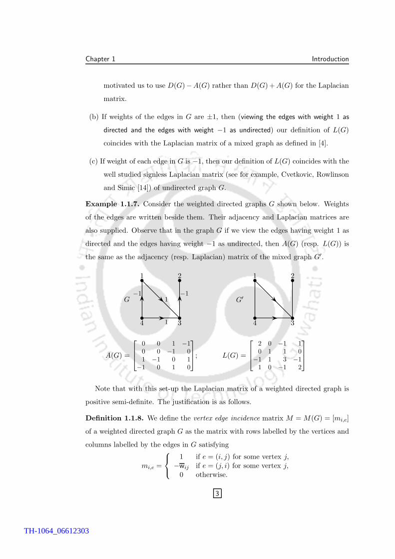
Example 1.1.7. Consider the weighted directed graphs G shown below. Weights
of the edges are written beside them. Their adjacency and Laplacian matrices are
also supplied. Observe that in the graph G if we view the edges having weight 1 as
directed and the edges having weight −1 as undirected, then A(G) (resp. L(G)) is
the same as the adjacency (resp. Laplacian) matrix of the mixed graph G′.
b
b
b
b
4 3
21
−1
1
−11G
b
b
b
b
4 3
21
G′
A(G) =
0 0 1 −10 0 −1 01 −1 0 1
−1 0 1 0
; L(G) =
2 0 −1 10 1 1 0
−1 1 3 −11 0 −1 2
Note that with this set-up the Laplacian matrix of a weighted directed graph is
positive semi-definite. The justification is as follows.
Definition 1.1.8. We define the vertex edge incidence matrix M = M(G) = [mi,e]
of a weighted directed graph G as the matrix with rows labelled by the vertices and
columns labelled by the edges in G satisfying
mi,e =
1 if e = (i, j) for some vertex j,−wij if e = (j, i) for some vertex j,
0 otherwise.
3
TH-1064_06612303
Chapter 1 Introduction
Notice that (MM∗)ii = di, and for i 6= j, (MM∗)ij = −wij if (i, j) ∈ E(G);
(MM∗)ij = −wji if (j, i) ∈ E(G); (MM∗)ij = 0 otherwise. Thus we see that
L(G) = MM∗, which implies the Laplacian matrix of a weighted directed graph is
positive semi-definite.
Observe that (M∗x)e = (x(i) − wijx(j)), for any x ∈ Cn and edge e = (i, j). It
follows that
x∗L(G)x = (M∗x)∗(M∗x) =∑
(i,j)∈E(G)
|x(i) − wijx(j)|2.�
�
�
�1.1.1
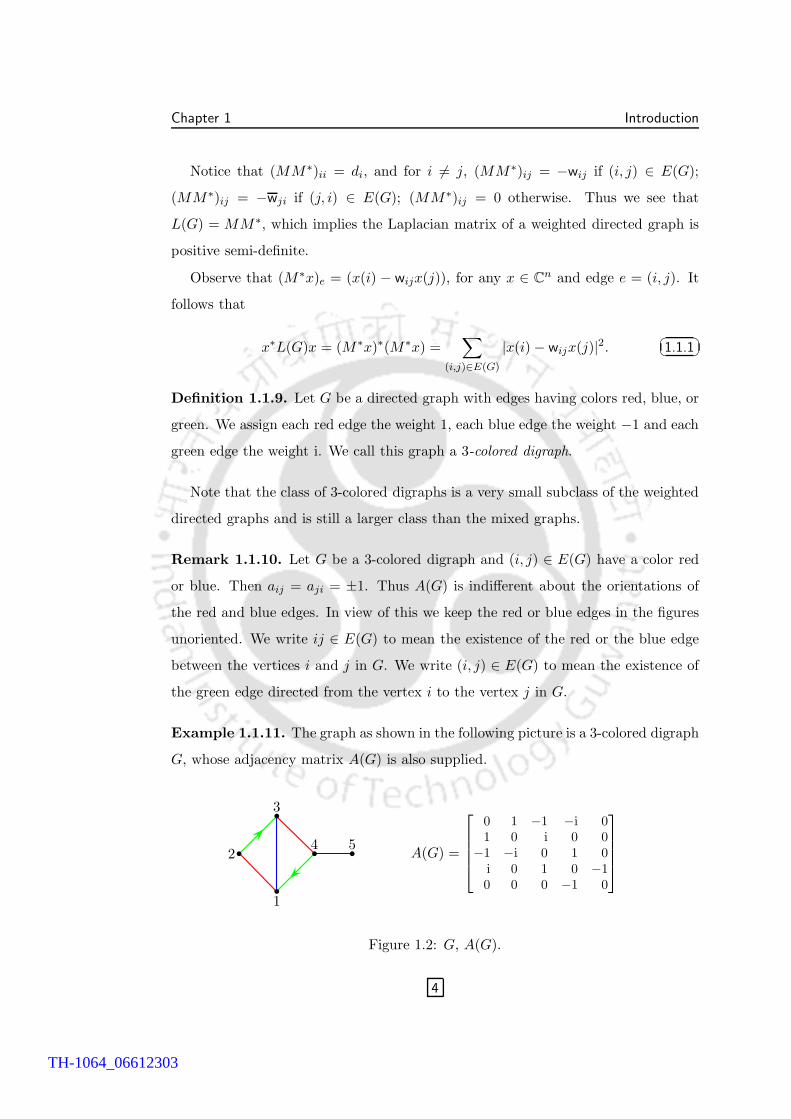
Definition 1.1.9. Let G be a directed graph with edges having colors red, blue, or
green. We assign each red edge the weight 1, each blue edge the weight −1 and each
green edge the weight i. We call this graph a 3-colored digraph.
Note that the class of 3-colored digraphs is a very small subclass of the weighted
directed graphs and is still a larger class than the mixed graphs.
Remark 1.1.10. Let G be a 3-colored digraph and (i, j) ∈ E(G) have a color red
or blue. Then aij = aji = ±1. Thus A(G) is indifferent about the orientations of
the red and blue edges. In view of this we keep the red or blue edges in the figures
unoriented. We write ij ∈ E(G) to mean the existence of the red or the blue edge
between the vertices i and j in G. We write (i, j) ∈ E(G) to mean the existence of
the green edge directed from the vertex i to the vertex j in G.
Example 1.1.11. The graph as shown in the following picture is a 3-colored digraph
G, whose adjacency matrix A(G) is also supplied.
1
2
3
4 5
b
b b
b
b A(G) =
0 1 −1 −i 01 0 i 0 0
−1 −i 0 1 0i 0 1 0 −10 0 0 −1 0
Figure 1.2: G, A(G).
4
TH-1064_06612303
Chapter 1 Introduction
Note that the usual Laplacian matrix of an unweighted undirected graph G, that
is, the Laplacian matrix of a weighted directed graph G with all edges having a
weight 1 is always singular. Fiedler [23] proved that 0 is a simple eigenvalue of L(G)
if and only if G is connected. Thus the second smallest eigenvalue of L(G) is positive
if and only if G is connected. Fiedler [23] termed the second smallest eigenvalue of
L(G) as the algebraic connectivity of G, henceforth we denote it by a(G). Here we
see a relationship between the spectral and structural properties of a graph. As
the term algebraic connectivity suggests, a(G) provides an algebraic measure of how
connected the graph G is. There is a wealth of results to support that statement,
beginning with the pioneering work of Fielder on the subject. An eigenvector of
L(G) corresponding to the algebraic connectivity is popularly known as a Fiedler
vector of G.
Definition 1.1.12. Let G be a weighted directed graph. The weight of a i1-ik-walk
W = [i1, . . . , ik] in G, denoted by wW is ai1i2ai2i3 . . . aik−1ik , where aij are the entries
of A(G). For 1 ≤ p ≤ k−1, if e = (ip, ip+1) ∈ E(G), then we say e is directed along
the walk, otherwise we say e is directed opposite to the walk.
Let G be a weighted directed graph and D = diag(d11, . . . , dnn) with |dii| = 1,
for each i. Then D∗A(G)D (resp. D∗L(G)D) is the adjacency (resp. Laplacian)
matrix of another weighted directed graph which we denote by DG. Observe that if
(i, j) ∈ E(G) has a weight wij , then it has the weight diiwijdjj in DG.
Definition 1.1.13. Let G and H be weighted directed graphs. We say H is D-
similar to G if there exists a diagonal matrix D (with |dii| = 1, for each i) such
that H = DG. Thus, both of them have the same undirected unweighted underlying
graph.
1.2 Organization of the Thesis
The thesis is organized as follows. There are five chapters in the thesis. Chapter 1
contains a brief introduction of the thesis and a few lines for motivation.
5
TH-1064_06612303
Chapter 1 Introduction
Chapter 2 is devoted mainly to the study of singularity of the Laplacian matrix
of weighted directed graphs. We show that singularity of the Laplacian matrix of
weighted directed graphs have close connection with the graph structure. We provide
a combinatorial description of the determinant of the Laplacian matrix of weighted
directed graphs relating the graph structure.
Chapter 3 deals with the adjacency and the Laplacian spectra of 3-colored di-
graphs. We show the realizability of the adjacency (resp. Laplacian) spectrum of
a 3-colored digraph as a subset of the adjacency (resp. Laplacian) spectrum of a
suitable undirected graph constructed by some graph operations on the 3-colored
digraph.
In Chapter 4 we study the smallest Laplacian eigenvalue and the corresponding
eigenvectors of 3-colored digraphs containing exactly one non-singular cycle. We dis-
cuss the non-singular unicyclic 3-colored digraphs, which minimize (resp. maximize)
the smallest Laplacian eigenvalue over all such graphs. Further, we characterize the
non-singular unicyclic 3-colored digraphs which have 1 as the second smallest Lapla-
cian eigenvalue.
An unweighted undirected graph G is bipartite if and only if −λ is an eigenvalue
of A(G) whenever λ is an eigenvalue of A(G), (see [13]). In contrast to this property
of bipartite graphs, Barik, Pati and Sarma [9] introduced the notion of graphs with
property (R), that is, the graphs satisfying the property that 1λ
is an eigenvalue of
A(G) whenever λ is an eigenvalue of A(G). Further, when λ and 1λ
are eigenvalues
of A(G) with the same multiplicity, then G is said to have SR-property. In [9],
the authors characterized all trees with SR-property and proved that a tree has
SR-property if and only if it is a simple corona tree. Barik et al. [7] studied the
structure of a unicyclic unweighted undirected graph with SR-property.
In Chapter 5 we determine the coefficients of the characteristic polynomial of the
adjacency matrix of 3-colored digraphs in terms of the graph structure. We supply
the structure of unicyclic 3-colored digraphs satisfying SR-property.
6
TH-1064_06612303
Chapter 2
Laplacian singularity of weighted directed graphs
In this chapter our focus is on the Laplacian matrix of weighted directed graphs and
its singularity. In Section 2.1 we supply several characterizations of singularity of
the Laplacian matrix of weighted directed graphs. This provides a better combina-
torial insight. Many results in this section generalize the known results related to
Laplacian singularity of the mixed graphs in the literature. We provide a charac-
terization of the connected weighted directed graphs which are D-similar to mixed
graphs, which is new of its kind. Tan and Fan [40] have introduced and studied the
parameter edge singularity of a mixed graph. In Section 2.2 we continue to study
the edge singularity for weighted directed graphs. The problem of characterizing
mixed graphs with a fixed edge singularity has never been addressed. We provide a
combinatorial characterization of connected weighted directed graphs having a fixed
edge singularity. In Section 2.3 we consider the class of 3-colored digraphs and sup-
ply some additional informations on the structure of singular connected 3-colored
digraphs, apart from that in section 2.1. In Section 2.4, we establish a relationship
between the determinant of the Laplacian matrix of weighted directed graphs and
the graph structure.
2.1 D-similarity and Laplacian singularity
It was first observed in [4], that unlike the usual Laplacian matrix of an undirected
graph, the Laplacian matrix of a mixed graph is sometimes non-singular. Several
characterizations of singularity for mixed graphs were provided in [4]. It is natural
to ask for similar characterization of singularity for the weighted directed graphs.
7
TH-1064_06612303
Chapter 2 Laplacian singularity of weighted directed graphs
Definition 2.1.1. We call a weighted directed graph singular (resp. non-singular)
if its Laplacian matrix is singular (resp. non-singular).
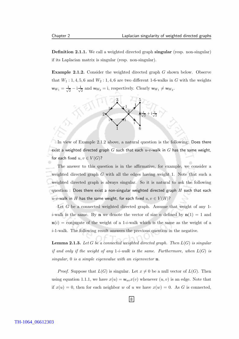
Example 2.1.2. Consider the weighted directed graph G shown below. Observe
that W1 : 1, 4, 5, 6 and W2 : 1, 4, 6 are two different 1-6-walks in G with the weights
wW1= 1√
2− i 1√
2and wW2
= i, respectively. Clearly wW16= wW2
.
b
b
b
b
b
b
1
2
3
4
5
6
i
−11
1i
1√2
+ i 1√2
1
In view of Example 2.1.2 above, a natural question is the following: Does there
exist a weighted directed graph G such that each u-v-walk in G has the same weight,
for each fixed u, v ∈ V (G)?
The answer to this question is in the affirmative, for example, we consider a
weighted directed graph G with all the edges having weight 1. Note that such a
weighted directed graph is always singular. So it is natural to ask the following
question : Does there exist a non-singular weighted directed graph H such that each
u-v-walk in H has the same weight, for each fixed u, v ∈ V (H)?
Let G be a connected weighted directed graph. Assume that weight of any 1-
i-walk is the same. By n we denote the vector of size n defined by n(1) = 1 and
n(i) = conjugate of the weight of a 1-i-walk which is the same as the weight of a
i-1-walk. The following result answers the previous question in the negative.
Lemma 2.1.3. Let G be a connected weighted directed graph. Then L(G) is singular
if and only if the weight of any 1-i-walk is the same. Furthermore, when L(G) is
singular, 0 is a simple eigenvalue with an eigenvector n.
Proof. Suppose that L(G) is singular. Let x 6= 0 be a null vector of L(G). Then
using equation 1.1.1, we have x(u) = wuvx(v) whenever (u, v) is an edge. Note that
if x(u) = 0, then for each neighbor w of u we have x(w) = 0. As G is connected,
8
TH-1064_06612303
Chapter 2 Laplacian singularity of weighted directed graphs
this implies that x = 0. Hence the eigenvalue 0 has multiplicity one. Let W be any
1-i-walk. Using equation 1.1.1, we have x(1) = wW x(i). Hence each 1-i-walk has
the same weight and x = x(1)n.
Conversely, suppose that the weight of any 1-i-walk is the same. Note that if
(i, j) ∈ E(G), then n(j) = wijn(i). Using equation (1.1.1), we have
n∗L(G)n =∑
(i,j)∈E(G)
|n(i) − wijn(j)|2 = 0.
Therefore ‖M∗n‖2 = 0 and L(G)n = MM∗n = 0. So L(G) is singular.
It follows that the class of singular connected weighted directed graphs is same
as the class of connected weighted directed graphs G satisfying the property that
each u-v-walk in G has the same weight, for each fixed u, v ∈ V (G).
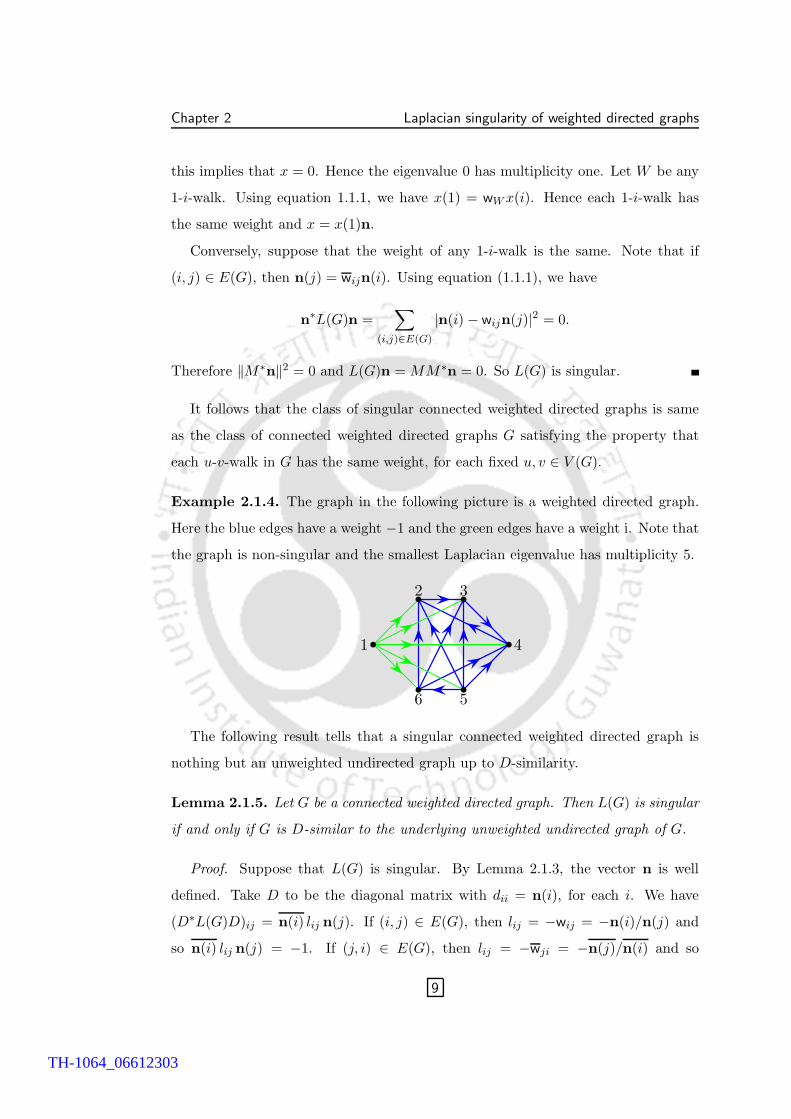
Example 2.1.4. The graph in the following picture is a weighted directed graph.
Here the blue edges have a weight −1 and the green edges have a weight i. Note that
the graph is non-singular and the smallest Laplacian eigenvalue has multiplicity 5.
b
b b
b
bb
1
2 3
4
56
The following result tells that a singular connected weighted directed graph is
nothing but an unweighted undirected graph up to D-similarity.
Lemma 2.1.5. Let G be a connected weighted directed graph. Then L(G) is singular
if and only if G is D-similar to the underlying unweighted undirected graph of G.
Proof. Suppose that L(G) is singular. By Lemma 2.1.3, the vector n is well
defined. Take D to be the diagonal matrix with dii = n(i), for each i. We have
(D∗L(G)D)ij = n(i) lij n(j). If (i, j) ∈ E(G), then lij = −wij = −n(i)/n(j) and
so n(i) lij n(j) = −1. If (j, i) ∈ E(G), then lij = −wji = −n(j)/n(i) and so
9
TH-1064_06612303
Chapter 2 Laplacian singularity of weighted directed graphs
n(i) lij n(j) = −1. Furthermore, lii = di implies n(i) lii n(i) = di. The converse is
trivial.
Remark 2.1.6. Notice that when G is a singular mixed graph, n is the vector with
entries 1 or −1. Hence in this case the diagonal matrix D in Lemma 2.1.5 is nothing
but a signature matrix.
Next result characterizes the singular cycles in a weighted directed graph. It will
be used to give another characterization of a non-singular weighted directed graph.
Lemma 2.1.7. Let C be a weighted directed graph whose underlying undirected
graph is a cycle. Then C is singular if and only if wC = 1.
Proof. If C is singular then by Lemma 2.1.3, we have 1 = wC . Conversely let
wC = 1 and W1 be a 1-i-path, i 6= 1. Let W2 be the other 1-i-path. Denote by W3
the i-1 path obtained by tracing back W2. Then 1 = wC = wW1wW3
, which implies
that wW1= 1/wW3
= wW2. Hence by Lemma 2.1.3, C is singular.
◮ In view of Lemma 2.1.7, we call a cycle C in a weighted directed graph singular
if its weight wC = 1. Otherwise we call it a non-singular cycle.
Remark 2.1.8. Notice that if we consider mixed graphs, then a cycle C is singular
if and only if wC = 1, that is there are an even number of undirected edges (viewing
the edges of weight −1 as undirected) on the cycle. That is the cycle is non-singular
if and only if it has an odd number undirected edges. So the previous lemma
generalizes Lemma 1 of [4].
The following result gives another characterization of singularity of a connected
weighted directed graph.
Lemma 2.1.9. Let G be a connected weighted directed graph. Then L(G) is singular
if and only if there exist a partition V (G) = V1 ∪ V2 · · · ∪ Vk such that the following
conditions are satisfied.
(i) There are distinct complex numbers wi of unit modulus associated with each Vi,
for i = 1, . . . , k,
10
TH-1064_06612303
Chapter 2 Laplacian singularity of weighted directed graphs
(ii) Any edge between Vi and Vj , i < j is either directed from Vi to Vj with a weight
wiwj 6= 1 or is directed from Vj to Vi with a weight wiwj 6= 1,
(iii) Each edge within Vi has a weight 1, for i = 1 . . . , k.
Proof. Suppose that L(G) is singular. By Lemma 2.1.3, 0 is a simple eigenvalue
and n is a null vector of L(G). Let Vi = {j ∈ V (G) : n(j) = n(i)}. Let u ∈ Vi,
v ∈ Vj and i < j such that (u, v) is an edge. If wuv = 1, then n(u) = n(v), which is
not possible. Since n(u) = n(i) and n(v) = n(j), we must have wuv = n(i)n(j) 6= 1,
by Lemma 2.1.3 and the definition of n. Similarly, if (v, u) is an edge, then we
must have wvu = n(j)n(i) 6= 1. So with each Vi we associate the complex number
wi = n(i). By definition of n, it is easy to see that edges within Vi have weights 1.
Conversely, suppose that V (G) = V1 ∪ V2 · · · ∪ Vk, and (i), (ii), (iii) are satis-
fied. Put D = diag(d11, . . . , dnn), where duu = wi if u ∈ Vi for some i. Note that
(D∗L(G)D)uv = duuluvdvv . If (u, v) ∈ E(G) has a weight 1, then (as the edges of
weight 1 appear only inside a Vi) both u, v ∈ Vi, for some i, where 1 ≤ i ≤ k. In
that case duu = dvv and luv = −1 which implies duuluvdvv = −1. If (u, v) ∈ E(G)
has a weight other than 1, then u ∈ Vi, v ∈ Vj, for some i, j, i 6= j. In that
case wuv = wiwj, by (ii). Thus duuluvdvv = wi(−wiwj)wj = −1. Furthermore,
duuluuduu = luu. Since D∗L(G)D is Hermitian, we see that D∗L(G)D is the Lapla-
cian matrix of the underlying unweighted undirected graph of G. Hence L(G) is
singular, by Lemma 2.1.5.
Remark 2.1.10. Notice that if we have mixed graph in Lemma 2.1.9, then we have
only two types of weights. Hence a connected mixed graph is singular if and only if
there exist a partition V (G) = V1 ∪ V2 such that edges inside Vi have weights 1 and
edges between V1 and V2 have weights −1.
The following theorem which is a summary of the previous discussions and is a
generalization of [4, Theorem 4].
Theorem 2.1.11. Let G be a connected weighted directed graph. Then the following
are equivalent.
11
TH-1064_06612303
Chapter 2 Laplacian singularity of weighted directed graphs
(a) L(G) is singular.
(b) G is D-similar to the underlying unweighted undirected graph of G.
(c) Each cycle C in G has weight wC = 1.
(d) There exist a partition V (G) = V1 ∪ · · · ∪ Vk such that the following conditions
are satisfied.
(i) There are distinct complex numbers wi of unit modulus associated with
each Vi, for i = 1, . . . , k,
(ii) Any edge between Vi and Vj , i < j is either directed from Vi to Vj with a
weight wiwj 6= 1 or is directed from Vj to Vi with a weight wiwj 6= 1,
(iii) Each edge within Vi has a weight 1, for i = 1 . . . , k.
Proof. (a) ⇔ (b). Follows from Lemma 2.1.5.
(b)⇔(c). Suppose that G is D-similar to the underlying unweighted undirected
graph of G. Consider DG for this D. Note that if (i, j) ∈ E(G) has a weight wij,
then it has the weight diiwijdjj in DG. So the weight of a cycle C in G remains the
same in DG. Note that each cycle in DG has weight 1. Hence the result holds.
Conversely suppose that each cycle in G has weight equal to 1. Let T be a
weighted directed spanning tree of G. Put d11 = 1 and for i > 1, dii = wPi, where
Pi is the unique i-1-path in T . Let D = diag(d11, . . . , dnn). Consider the graph DG
whose Laplacian matrix is D∗L(G)D. Take an edge (i, j) ∈ E(G). If (i, j) ∈ E(T ),
then djj = wijdii. In that case (D∗L(G)D)ij = diilijdjj = −1. Thus weight of (i, j)
is 1 in DG. If (i, j) ∈ E(G) − E(T ), then consider the cycle C = P + (i, j) in G,
where P is the unique i-j-path in T . Thus wC = wijwP . Observe that, weight of a
cycle in G remains the same in DG. Thus weight of (i, j) must be 1 in DG, as wP is
equal to 1 in DG and wC = 1. Hence DG is the underlying unweighted undirected
graph of G.
(b)⇔(d). Follows from Lemma 2.1.9.
The following result is an immediate consequence.
12
TH-1064_06612303
Chapter 2 Laplacian singularity of weighted directed graphs
Corollary 2.1.12. Let G be a connected weighted directed graph. Then G is non-
singular if and only if it contains a non-singular cycle. In particular, a weighted
directed tree is always singular.
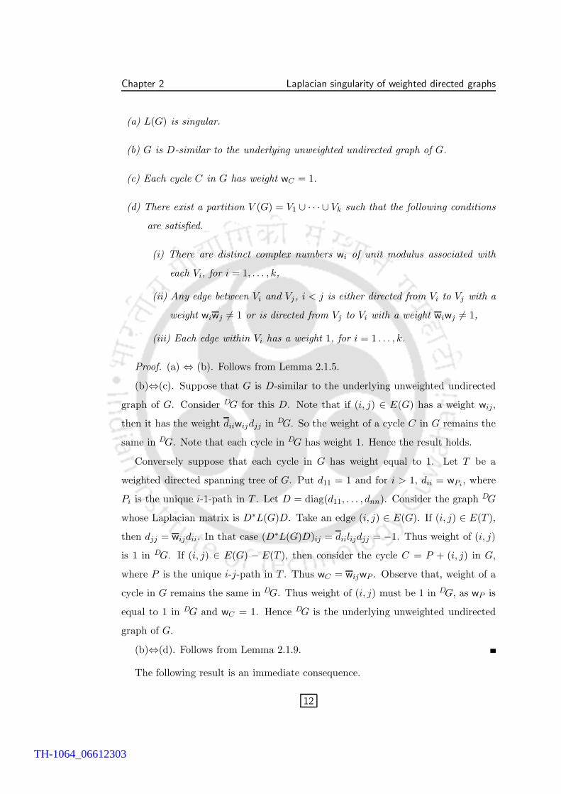
Example 2.1.13. Consider G as in the following picture. Note that there are two
cycles in G and both of them have weight 1. Hence the graph is singular. Indeed one
can check that n =[1 − 1√
2+ i√
2i −i −i −1 i −i −1 −i
]tis a null vector
of L(G).
b
b
b b
b
b
b b
b
b
G
ii
−11−1
1√2
+ i√2
i
i
1
−1
i
1
2
3 4
5
6
7 8
9
10
Observe that in the above picture, if we take the directed edge (9, 8) instead of (8, 9),
then the weight of the cycle [8, 10, 9, 8] becomes −1. Hence by Corollary 2.1.12, the
graph is non-singular.
Note that by Lemma 2.1.5, a connected weighted directed graph is singular if and
only if it is D-similar to an unweighted undirected graph. The following is a natural
question: which connected weighted directed graphs are D-similar to mixed graphs?
Next result characterizes those graphs.
Theorem 2.1.14. Let G be a connected weighted directed graph. Then G is D-
similar to a mixed graph if and only if G does not contain a cycle of non-real weight.
Proof. Suppose that G does not contain a cycle of non-real weight. Then each
of the cycle contained in G has a weight ±1, as the weights of the edges have
absolute value 1. Let T be a weighted directed spanning tree of G. By Corollary
2.1.12, T is singular. By Lemma 2.1.5, there is a diagonal matrix D, such that
DT is an unweighted undirected tree. Consider the graph DG for this D. Take an
edge (i, j) ∈ E(G). If (i, j) ∈ E(T ), then weight of (i, j) is equal to 1 in DG. If
(i, j) ∈ E(G) −E(T ), then consider the cycle C = P + (i, j), where P is the unique
13
TH-1064_06612303
Chapter 2 Laplacian singularity of weighted directed graphs
i-j-path in T . Since the edges in DG corresponding to the edges in P have weight 1,
we see that wP is equal to 1 in DG. Observe that the weight of a cycle in G remains
the same in DG. Thus the weight of (i, j) is either 1 or −1 in DG, as wC = ±1.
Hence the DG is a mixed graph.
Conversely, suppose that G is D-similar to a mixed graph H. So L(H) =
D∗L(G)D and H=DG. As the weight of a cycle is the same in both G and DG,
we see that the weights of the cycles are real.
2.2 Edge singularity of weighted directed graph
The edge singularity of mixed graphs was studied in [40]. We continue the same
study in the context of weighted directed graphs.
Definition 2.2.1. The edge singularity εs(G) of a weighted directed graph is the
minimum number of edges whose removal results a weighted directed graph contain-
ing no non-singular cycles or cycles of weight different from 1 (by Lemma 2.1.7).
That is, all components of the resulting graph are singular.
The following result is very fundamental in nature and it relates the edge singu-
larity with connectivity.
Lemma 2.2.2. Let G be a connected weighted directed graph. Let F be a set of
εs(G) edges in G such that G − F does not contain a cycle of weight different from
1. Then G − F is connected.
Proof. If G is singular, then the result holds obviously. Suppose that G is non-
singular and G − F is disconnected. Let G1, G2, . . . Gr, (r ≥ 2) be the components
of G − F . As the graph G is connected, we can choose r − 1 edges e1, e2, . . . er−1
from F such that the graph
H := G1 ∪ G2 ∪ . . . Gr + {e1, e2, . . . er−1}
is connected. So each edge e1, . . . , er−1 must be a bridge in H. By Corollary 2.1.12,
as Gi’s do not contain non-singular cycles, we see that H does not contain a non-
14
TH-1064_06612303
Chapter 2 Laplacian singularity of weighted directed graphs
singular cycle. Thus H is singular, by Corollary 2.1.12. Hence εs(G) ≤ |F |−(r−1) <
|F |, a contradiction.
The following result generalizes [40, Theorem 2.1] obtained by Tan and Fan for
mixed graphs.
Lemma 2.2.3. Let G be a connected weighted directed graph on n vertices and m
edges. Then 0 ≤ εs(G) ≤ m − n + 1. In particular, εs(G) = m − n + 1 if and only
if all the cycles contained in G are non-singular.
Proof. Clearly, εs(G) ≥ 0. Let T be a spanning tree of G. By Corollary 2.1.12,
T is singular. Thus removal of the m − n + 1 edges which are not in T from the
graph G makes the resulting graph singular. Hence εs(G) ≤ m − n + 1.
Suppose that εs(G) = m−n+1 and G contains a singular cycle C. Let H be the
unicyclic spanning subgraph of G containing the cycle C. By Corollary 2.1.12, H is
singular. Thus by deleting the m − n edges from G we obtain a singular weighted
directed graph. Hence εs(G) ≤ m − n < m − n + 1, a contradiction.
Conversely, suppose that each of the cycles contained in G are non-singular and
εs(G) < m − n + 1. Let F be a set of εs(G) edges in G such that the graph G − F
has each component singular. By Lemma 2.2.2, G − F is a connected graph and
|E(G−F )| = m−εs(G) > n−1. Thus G−F contains a cycle, and by the assumption
this cycle is non-singular, a contradiction. Hence the result holds.
We have two natural questions.
a) Given a non-negative integer k, is it possible to find a graph G with εs(G) = k?
b) Given n,m and an integer 0 ≤ k ≤ m − n + 1, does there exist a graph G with n
vertices and m edges for which εs(G) = k?
The following example answers the first question in the affirmative.
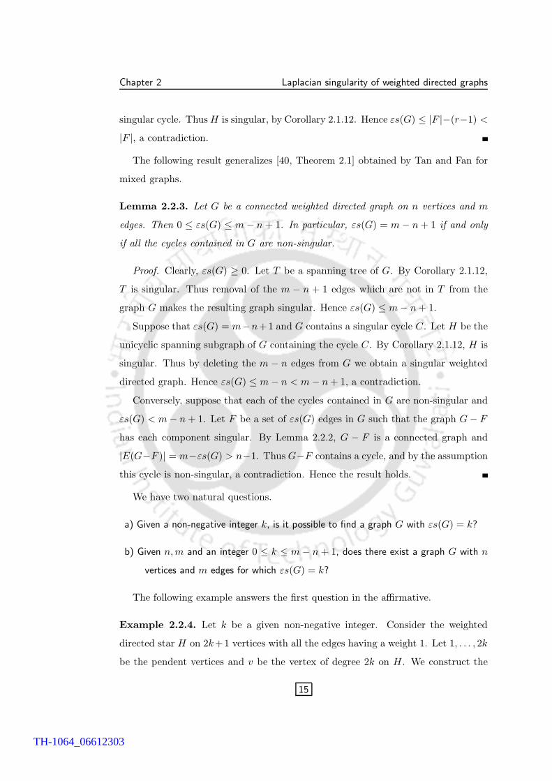
Example 2.2.4. Let k be a given non-negative integer. Consider the weighted
directed star H on 2k+1 vertices with all the edges having a weight 1. Let 1, . . . , 2k
be the pendent vertices and v be the vertex of degree 2k on H. We construct the
15
TH-1064_06612303
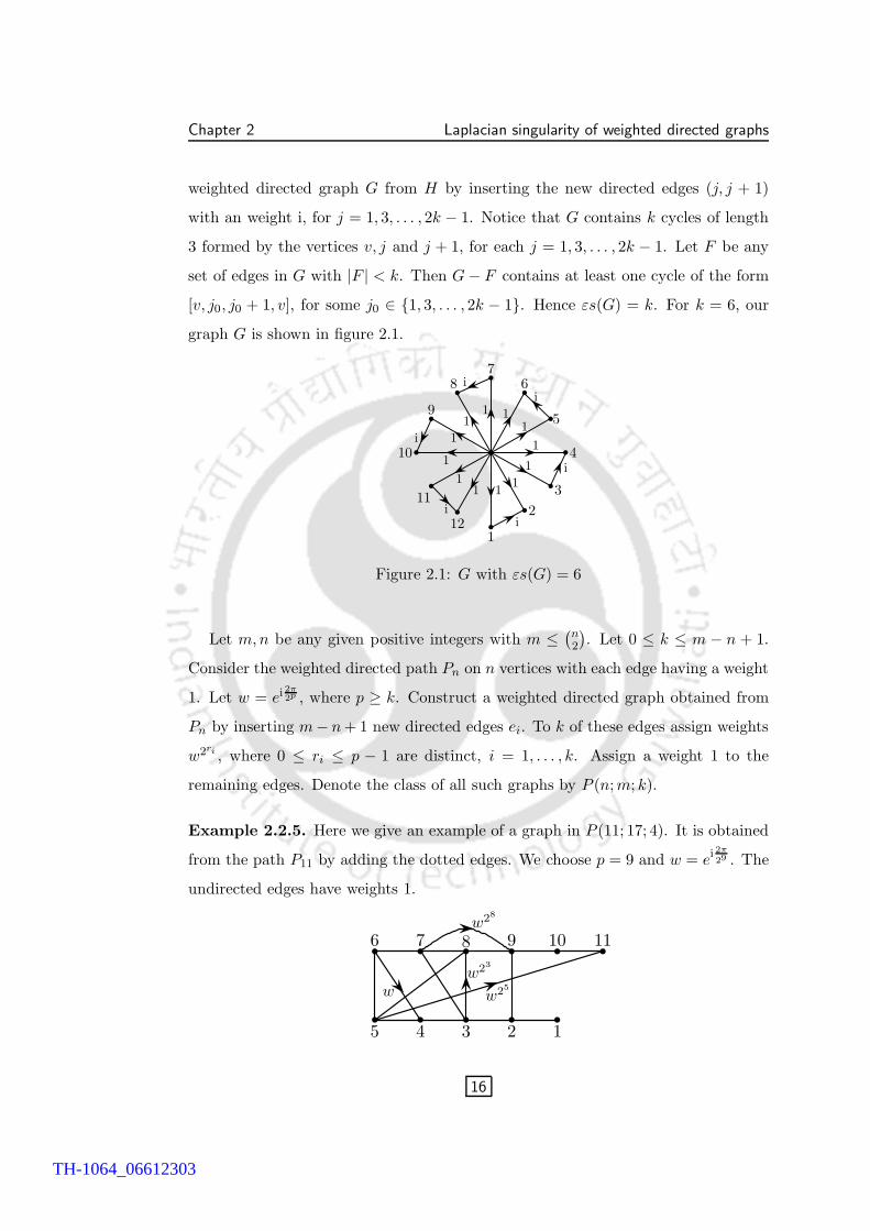
Chapter 2 Laplacian singularity of weighted directed graphs
weighted directed graph G from H by inserting the new directed edges (j, j + 1)
with an weight i, for j = 1, 3, . . . , 2k − 1. Notice that G contains k cycles of length
3 formed by the vertices v, j and j + 1, for each j = 1, 3, . . . , 2k − 1. Let F be any
set of edges in G with |F | < k. Then G − F contains at least one cycle of the form
[v, j0, j0 + 1, v], for some j0 ∈ {1, 3, . . . , 2k − 1}. Hence εs(G) = k. For k = 6, our
graph G is shown in figure 2.1.
b
b
b
bb
b
b
b
b
b
b
b
b
i
i
ii
i
i
1
1
11
1
1
11
1
1
11
1
2
3
4
5
67
8
9
10
11
12
Figure 2.1: G with εs(G) = 6
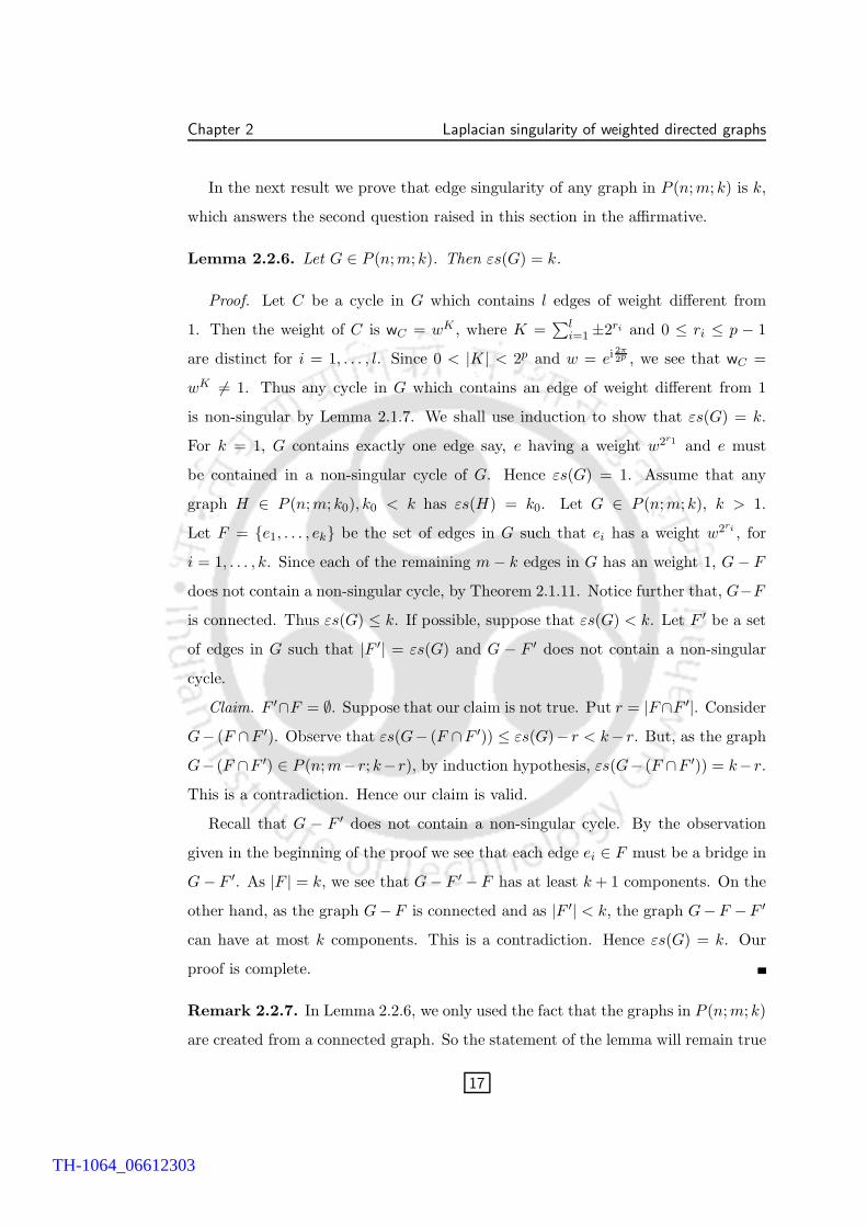
Let m,n be any given positive integers with m ≤(n2
). Let 0 ≤ k ≤ m − n + 1.
Consider the weighted directed path Pn on n vertices with each edge having a weight
1. Let w = ei 2π2p , where p ≥ k. Construct a weighted directed graph obtained from
Pn by inserting m− n + 1 new directed edges ei. To k of these edges assign weights
w2ri , where 0 ≤ ri ≤ p − 1 are distinct, i = 1, . . . , k. Assign a weight 1 to the
remaining edges. Denote the class of all such graphs by P (n;m; k).
Example 2.2.5. Here we give an example of a graph in P (11; 17; 4). It is obtained
from the path P11 by adding the dotted edges. We choose p = 9 and w = ei 2π
29 . The
undirected edges have weights 1.
b bbbbb
bbbbb
12345
6 7 8 9 10 11
w
w28
w23
w25
16
TH-1064_06612303
Chapter 2 Laplacian singularity of weighted directed graphs
In the next result we prove that edge singularity of any graph in P (n;m; k) is k,
which answers the second question raised in this section in the affirmative.
Lemma 2.2.6. Let G ∈ P (n;m; k). Then εs(G) = k.
Proof. Let C be a cycle in G which contains l edges of weight different from
1. Then the weight of C is wC = wK , where K =∑l
i=1 ±2ri and 0 ≤ ri ≤ p − 1
are distinct for i = 1, . . . , l. Since 0 < |K| < 2p and w = ei 2π2p , we see that wC =
wK 6= 1. Thus any cycle in G which contains an edge of weight different from 1
is non-singular by Lemma 2.1.7. We shall use induction to show that εs(G) = k.
For k = 1, G contains exactly one edge say, e having a weight w2r1 and e must
be contained in a non-singular cycle of G. Hence εs(G) = 1. Assume that any
graph H ∈ P (n;m; k0), k0 < k has εs(H) = k0. Let G ∈ P (n;m; k), k > 1.
Let F = {e1, . . . , ek} be the set of edges in G such that ei has a weight w2ri , for
i = 1, . . . , k. Since each of the remaining m − k edges in G has an weight 1, G − F
does not contain a non-singular cycle, by Theorem 2.1.11. Notice further that, G−F
is connected. Thus εs(G) ≤ k. If possible, suppose that εs(G) < k. Let F ′ be a set
of edges in G such that |F ′| = εs(G) and G − F ′ does not contain a non-singular
cycle.
Claim. F ′∩F = ∅. Suppose that our claim is not true. Put r = |F∩F ′|. Consider
G− (F ∩F ′). Observe that εs(G− (F ∩F ′)) ≤ εs(G)− r < k− r. But, as the graph
G− (F ∩F ′) ∈ P (n;m−r; k−r), by induction hypothesis, εs(G− (F ∩F ′)) = k−r.
This is a contradiction. Hence our claim is valid.
Recall that G − F ′ does not contain a non-singular cycle. By the observation
given in the beginning of the proof we see that each edge ei ∈ F must be a bridge in
G − F ′. As |F | = k, we see that G− F ′ − F has at least k + 1 components. On the
other hand, as the graph G−F is connected and as |F ′| < k, the graph G−F −F ′
can have at most k components. This is a contradiction. Hence εs(G) = k. Our
proof is complete.
Remark 2.2.7. In Lemma 2.2.6, we only used the fact that the graphs in P (n;m; k)
are created from a connected graph. So the statement of the lemma will remain true
17
TH-1064_06612303
Chapter 2 Laplacian singularity of weighted directed graphs
for graphs in T (n;m; k) which are created from a tree T in a similar way.
The graphs in P (n;m; k) may be viewed as some graphs obtained from a con-
nected undirected graph by adding k edges of weight different from 1. So a natural
question is the following: is it true that each connected weighted directed graph G with
εs(G) = k can be created from a connected unweighted undirected graph by adding k
directed edges of weight different from 1?
The answer is in the affirmative as shown below.
Theorem 2.2.8. Let G be a connected weighted directed graph with εs(G) = k.
Then G is D-similar to a graph H, obtained from the underlying unweighted graph
of G by assigning weights different from 1 to some k edges.
Proof. Let F be a set of edges in G such that |F | = εs(G) and G − F has each
component singular. By Lemma 2.2.2, the graph G− F is connected. Let D be the
diagonal matrix with i-th diagonal entry dii = n(i), where n is the null vector of
G − F . By Lemma 2.1.5, G − F is D-similar to the unweighted undirected graph
H0 := DG − DF , where DF is the set of edges in DG corresponding to F . Note that
H0 is connected as G − F is connected. As εs(G) = εs(DG), we see that edges in
DF must have weights other than 1. Put H=DG. Then the graph G is D-similar to
H which can be obtained from the connected unweighted graph H0 by adding the
k directed edges contained in DF .
2.3 3-colored digraphs and their singularity
Recall that the class of 3-colored digraphs contains the mixed graphs but is a small
subclass of the class of weighted directed graphs. In Section 2.1, we have given some
characterizations of a singular connected weighted directed graphs. In this section
we supply some additional characterizations of singularity of connected 3-colored
digraphs. Further information on the structure of a singular connected 3-colored
digraph is obtained.
18
TH-1064_06612303
Chapter 2 Laplacian singularity of weighted directed graphs
Remark 2.3.1. In particular, if a 3-colored digraph G does not contain a green edge,
then G is nothing but a mixed graph. In that case an edge with color red corresponds
to a directed edge and an edge with color blue corresponds to an undirected edge.
The following theorem provides some additional information on the the struc-
ture of singular connected 3-colored digraphs in comparison to Lemma 2.1.9. It
generalizes the result about the structure of a singular mixed graph obtained in [4].
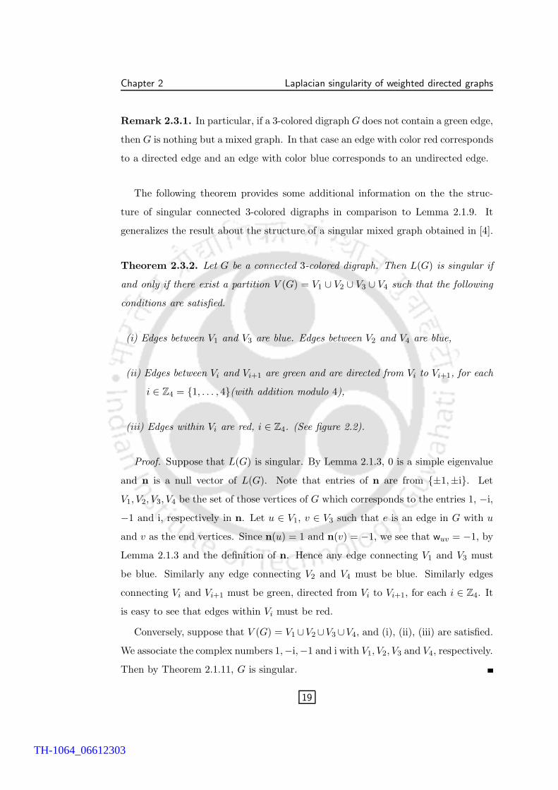
Theorem 2.3.2. Let G be a connected 3-colored digraph. Then L(G) is singular if
and only if there exist a partition V (G) = V1 ∪ V2 ∪ V3 ∪ V4 such that the following
conditions are satisfied.
(i) Edges between V1 and V3 are blue. Edges between V2 and V4 are blue,
(ii) Edges between Vi and Vi+1 are green and are directed from Vi to Vi+1, for each
i ∈ Z4 = {1, . . . , 4}(with addition modulo 4),
(iii) Edges within Vi are red, i ∈ Z4. (See figure 2.2).
Proof. Suppose that L(G) is singular. By Lemma 2.1.3, 0 is a simple eigenvalue
and n is a null vector of L(G). Note that entries of n are from {±1,±i}. Let
V1, V2, V3, V4 be the set of those vertices of G which corresponds to the entries 1, −i,
−1 and i, respectively in n. Let u ∈ V1, v ∈ V3 such that e is an edge in G with u
and v as the end vertices. Since n(u) = 1 and n(v) = −1, we see that wuv = −1, by
Lemma 2.1.3 and the definition of n. Hence any edge connecting V1 and V3 must
be blue. Similarly any edge connecting V2 and V4 must be blue. Similarly edges
connecting Vi and Vi+1 must be green, directed from Vi to Vi+1, for each i ∈ Z4. It
is easy to see that edges within Vi must be red.
Conversely, suppose that V (G) = V1 ∪V2∪V3 ∪V4, and (i), (ii), (iii) are satisfied.
We associate the complex numbers 1,−i,−1 and i with V1, V2, V3 and V4, respectively.
Then by Theorem 2.1.11, G is singular.
19
TH-1064_06612303
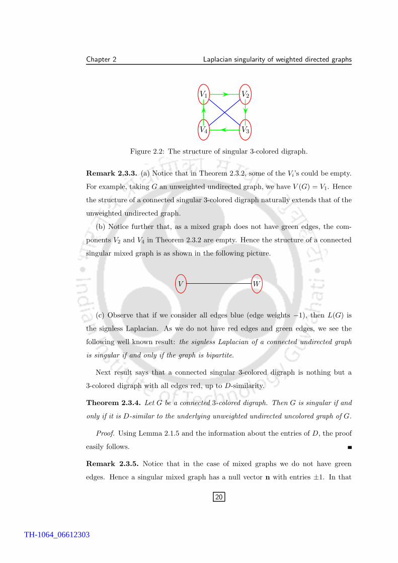
Chapter 2 Laplacian singularity of weighted directed graphs
V1 V2
V3V4
Figure 2.2: The structure of singular 3-colored digraph.
Remark 2.3.3. (a) Notice that in Theorem 2.3.2, some of the Vi’s could be empty.
For example, taking G an unweighted undirected graph, we have V (G) = V1. Hence
the structure of a connected singular 3-colored digraph naturally extends that of the
unweighted undirected graph.
(b) Notice further that, as a mixed graph does not have green edges, the com-
ponents V2 and V4 in Theorem 2.3.2 are empty. Hence the structure of a connected
singular mixed graph is as shown in the following picture.
V W
(c) Observe that if we consider all edges blue (edge weights −1), then L(G) is
the signless Laplacian. As we do not have red edges and green edges, we see the
following well known result: the signless Laplacian of a connected undirected graph
is singular if and only if the graph is bipartite.
Next result says that a connected singular 3-colored digraph is nothing but a
3-colored digraph with all edges red, up to D-similarity.
Theorem 2.3.4. Let G be a connected 3-colored digraph. Then G is singular if and
only if it is D-similar to the underlying unweighted undirected uncolored graph of G.
Proof. Using Lemma 2.1.5 and the information about the entries of D, the proof
easily follows.
Remark 2.3.5. Notice that in the case of mixed graphs we do not have green
edges. Hence a singular mixed graph has a null vector n with entries ±1. In that
20
TH-1064_06612303
Chapter 2 Laplacian singularity of weighted directed graphs
case the diagonal matrix D in Theorem 2.3.4 is nothing but a signature matrix.
Thus Theorem 2.3.4 is a generalization of Theorem 4 (iii) of [4].
Let C = [i1, . . . , ik, i1] be a cycle contained in a 3-colored digraph G. Let nb(C)
denote the number of blue edges in C. Let n+g (C) and n−
g (C) denote the number of
green edges in C which are directed along the cycle and the number of green edges
in C which are directed opposite to the cycle, respectively. The following result
is crucial for another characterization of singularity for 3-colored digraphs which is
done next.
Lemma 2.3.6. Let G be a 3-colored digraph whose underlying undirected graph is
a cycle C. Then G is singular if and only if
(a) either nb(C) is even and n+g (C) − n−
g (C) ≡ 0 (mod 4), or
(b) nb(C) is odd and n+g (C) − n−
g (C) ≡ 2 (mod 4).
Proof. Using Lemma 2.1.7, L(G) is singular if and only if
1 = wC = (−1)nb(C)in+g (C)(−i)n
−
g (C) = (−1)nb(C)in+g (C)−n−
g (C),
which implies the result.
Remark 2.3.7. Note that Theorem 2.3.2, Theorem 2.3.4 and Lemma 2.3.6 together
naturally generalizes [4, Theorem 4].
Next theorem gives a characterization of connected non-singular 3-colored di-
graphs.
Theorem 2.3.8. Let G be a connected 3-colored digraph. Then G is non-singular
if and only if G contains a cycle C satisfying one of the following conditions:
(a) n+g (C) − n−
g (C) ≡ 1 (mod 2),
(b) nb(C) is even and n+g (C) − n−
g (C) ≡ 2 (mod 4), or
(c) nb(C) is odd and n+g (C) − n−
g (C) ≡ 0 (mod 4).
21
TH-1064_06612303
Chapter 2 Laplacian singularity of weighted directed graphs
Proof. Suppose that G is non-singular. By Corollary 2.1.12, G contains a non-
singular cycle, say C. Hence by Lemma 2.3.6, it follows that the cycle C satisfies
one of the conditions (a), (b) or (c).
Conversely, suppose that G contains a cycle C satisfying one of the conditions
(a), (b) or (c). Then by Lemma 2.3.6, the cycle C is non-singular. Hence G is
non-singular, by Corollary 2.1.12.
Remark 2.3.9. Notice that in the case of mixed graphs we do not have green
edges. Hence a mixed graph whose underlying undirected graph is a cycle is non-
singular if and only if nb(C) is odd. Thus in view of remark 2.3.1, Theorem 2.3.8 is
a generalization of Lemma 1 of [4].
2.4 Determinant of the Laplacian matrix of weighted
directed graph
In this section we describe the determinant of the Laplacian matrix of a weighted
directed graph. The following lemma gives the determinant of the Laplacian matrix
of a cycle in a weighted directed graph.
Lemma 2.4.1. Let C be a weighted directed graph whose underlying unweighted
undirected graph is a cycle. Then det(L(C)) = 2(1 − RewC).
Proof. Consider the vertex edge incident matrix M(C) corresponding to C. We
may assume C = [1, 2, . . . , n, 1] such that the edges ei in C has end vertices i and
i + 1, for i ∈ Zn and m1,e1= 1, after a relabelling of the vertices if necessary. Note
that the nonzero entries of M(C) occurs precisely at the positions mi,eiand mi+1,ei
for each i. In that case expanding along the first row of M(C), we see that
det(M(C)) =∏
(i+1,i)∈E(C)i∈Zn
(−wi+1,i) − (−1)n∏
(i,i+1)∈E(C)i∈Zk
(−wi,i+1)
Since L(C) = M(C)M(C)∗, we see that det(L(C)) = 2(1 − RewC).
Next lemma gives the determinant of the Laplacian matrix of a unicyclic weighted
directed graph.
22
TH-1064_06612303
Chapter 2 Laplacian singularity of weighted directed graphs
Lemma 2.4.2. Let G be a connected unicyclic weighted directed graph with the cycle
C. Then det(L(G)) = 2(1 − RewC).
Proof. If G is the cycle C itself then the result follows immediately from Lemma
2.4.1. Otherwise, G has a pendent vertex say i. Let j be the vertex adjacent to i in
G with an edge e of weight w. We may assume, after a permutation similarity that
the first row and the first column of M(G) correspond to the vertex i and the edge
e, respectively. Then expanding along the first row, we see that if e = (i, j) then
det(M(G)) = det(M(G′)), otherwise det(M(G)) = (−w) det(M(G′)), where G′ is
the weighted directed graph obtained from G by deleting the vertex i. Hence in any
case det(L(G)) = det(L(G′)). Continuing similarly, after finitely many steps we see
that det(L(G)) = det(L(C)). Hence the result holds, by Lemma 2.4.1.
Definition 2.4.3. Let G be a connected non-singular weighted directed graph. We
call a subgraph H an essential spanning subgraph of G if V (G) = V (H) and every
component of H is a non-singular unicyclic weighted directed graph. By E(G) we
denote the class of all essential spanning subgraphs of G.
Next result describes the determinant of the Laplacian matrix of a weighted
directed graph in terms of the determinants of its essential spanning subgraphs.
Lemma 2.4.4. Let G be a connected weighted directed graph. Then det(L(G)) =∑
H∈E(G)
detL(H).
Proof. Since L(G) = MM∗, by Cauchy-Binet Theorem we know that
detL(G) =∑
E′⊆E|E′|=n
det M [V,E′] det M [V,E′]∗,
where M [V,E′] is a square submatrix of M . Note that M [V,E′] is the vertex edge
incident matrix of the spanning subgraph say HE′ with the edge set E′ ⊆ E. Thus
L(HE′) = M [V,E′]M [V,E′]∗. Note that detL(HE′) 6= 0 if and only if each com-
ponent of HE′ is non-singular. Thus det L(H ′E) 6= 0 if and only if HE′ ∈ E(G), as
|V | = |E′|. Hence the result holds.
23
TH-1064_06612303
Chapter 2 Laplacian singularity of weighted directed graphs
Remark 2.4.5. L(G) is non-singular if and only if G contains a non-singular cycle.
◮ Let G be a weighted directed graph and let H be an essential spanning subgraph
of G. We denote the number of components of H by ω(H) and a cycle contained in
H by Ci(H), for 1 ≤ i ≤ ω(H).
Next, we give our main result of this section, which generalizes [4, Corollary 2].
Theorem 2.4.6. Let G be a connected non-singular weighted directed graph. Then
det(L(G)) =∑
H∈E(G)
2ω(H)
ω(H)∏
i=1
(1 − RewCi(H)).
Proof. Proof follows from Lemma 2.4.4 and Lemma 2.4.2.
The following result is an immediate consequence.
Corollary 2.4.7. Let G be a connected 3-colored digraph. Then
detL(G) =∑
H∈E(G)
22ω1(H)+ω2(H),
where ω1(H) and ω2(H) denotes the number of cycles of weight −1 and ±i in H,
respectively.
24
TH-1064_06612303
Chapter 3
Spectra of 3-colored Digraphs
In this chapter we discuss the adjacency and Laplacian spectra of 3-colored digraphs.
In Section 3.1, we study the realizability of the adjacency (resp. Laplacian) spectrum
of a 3-colored digraph as a subset of the adjacency (resp. Laplacian) spectrum of a
mixed graph. Using a graph operation (on 3-colored digraphs) similar to that in [17]
we show that given a connected 3-colored digraph G on n vertices, there is a mixed
graph G[g] on 2n vertices, which satisfy both these requirements simultaneously.
In Section 3.2 we study the realizability of the adjacency (resp. Laplacian) spec-
trum of a mixed graph as a subset of the adjacency (resp. Laplacian) spectrum of
an unweighted undirected graph. Note that some study on the Laplacian spectrum
has been done by Zhang and Luo[42] and Fan [17, 18, 19, 20]. Using the graph oper-
ation (on mixed graphs) given in [17] we show that given a connected mixed graph
G on n vertices, there is an unweighted undirected graph G[b] on 2n vertices, which
satisfy both these requirements. We establish a relationship between the singularity
of L(G) and the connectedness of the graph G[b]. We give complete characterization
of the adjacency and Laplacian spectrum of G[b]. Denote by λi(B) the ith smallest
eigenvalue of a Hermitian matrix B. A family of mixed graphs G for which L(G) is
non-singular and λ1(L(G)) = λ2(L(G[b])) was provided by Fan [17]. A larger family
was supplied by Tan and Fan[40]. We provide a more general class of such mixed
graphs.
Combining the results of sections 3.1 and 3.2, we see that given a 3-colored
digraph G, there is an unweighted undirected graph H such that the adjacency
(resp. Laplacian) spectrum of H contains the adjacency (resp. Laplacian) spectrum
of G. We observe that the graph H may also be viewed as the result of a special
25
TH-1064_06612303
Chapter 3 Spectra of 3-colored Digraphs
case of a graph operation on unweighted undirected graphs which we introduce in
Section 3.3. This graph operation is more general than those discussed in sections
3.1 and 3.2 and is a new of its kind. We give a complete characterization of the
adjacency (resp. Laplacian) spectrum of the graph resulting from such operation.
3.1 Mixed Graphs whose spectrum contains the spec-
trum of a given 3-colored digraph
In this section we ask the following question: Let G be a 3-colored digraph. Is it
possible to find a mixed graph H1 whose adjacency spectrum is the same as that of G,
not considering multiplicities? Is it possible to find a mixed graph H2 whose Laplacian
spectrum is the same as that of G, not considering multiplicities? In case both the
answers are ‘yes’, is it possible to have H1 = H2? In this section we show that the
answers to all these questions are in the affirmative.
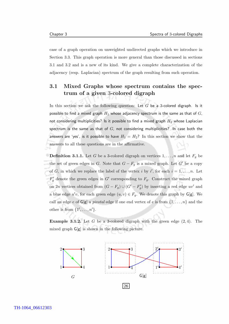
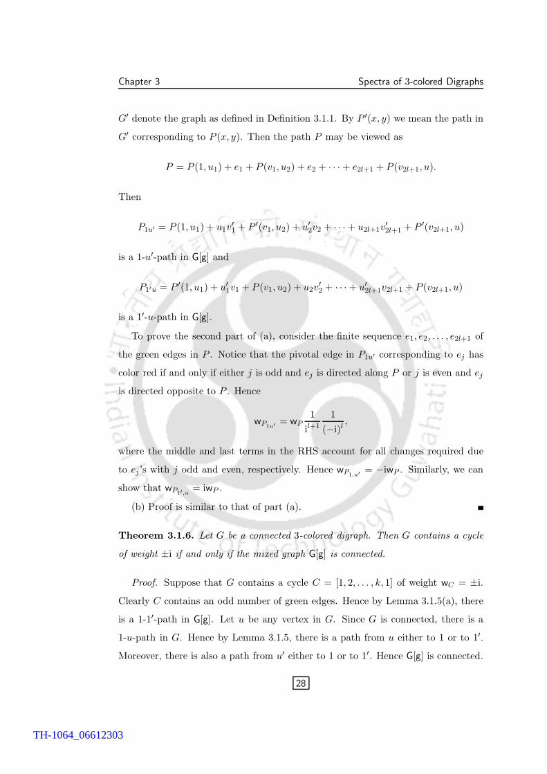
Definition 3.1.1. Let G be a 3-colored digraph on vertices 1, . . . , n and let Fg be
the set of green edges in G. Note that G − Fg is a mixed graph. Let G′ be a copy
of G, in which we replace the label of the vertex i by i′, for each i = 1, . . . , n. Let
F ′g denote the green edges in G′ corresponding to Fg. Construct the mixed graph
on 2n vertices obtained from (G − Fg) ∪ (G′ − F ′g) by inserting a red edge uv′ and
a blue edge u′v, for each green edge (u, v) ∈ Fg. We denote this graph by G[g]. We
call an edge e of G[g] a pivotal edge if one end vertex of e is from {1, . . . , n} and the
other is from {1′, . . . , n′}.
Example 3.1.2. Let G be a 3-colored digraph with the green edge (2, 4). The
mixed graph G[g] is shown in the following picture.
1
2 3
4
G
b
b b
b 1
2 3
4b
b b
b 1′
2′ 3′
4′b
b b
b
G[g]
26
TH-1064_06612303
Chapter 3 Spectra of 3-colored Digraphs
For two disjoint subsets of vertices U and V of a graph G, let E(U, V ) denote the
set of edges in G with one end in U and the other end in V .
Lemma 3.1.3. Let G be a connected 3-colored digraph such that Fg 6= ∅ and that G
does not contain a cycle of weight ±i. Then G − Fg is disconnected. Furthermore,
there is a partition V (G) = V1 ∪ V2 such that E(V1, V2) = Fg.
Proof. If possible, suppose that G−Fg is connected. Let e ∈ Fg. Then the graph
G− Fg + e has a cycle, say C which contains the green edge e. Thus we get a cycle
in G of weight ±i, which is a contradiction.
Let G1, . . . , Gk be the connected components of G − Fg. Note that there cannot
be any green edge between two vertices of G1, otherwise we get a cycle of weight ±i
in G.
Consider the graph H obtained from G − Fg by compressing Gi to a vertex vi,
adding an edge between vi and vj if there is a green edge between a vertex of Gi and
a vertex of Gj in G. The graph H cannot have an odd cycle, otherwise we would
get a cycle in G of weight ±i. Hence H is bipartite, say V (H) = W1 ∪ W2.
Put V1 =⋃
vi∈W1
V (Gi) and V2 =⋃
vi∈W2
V (Gi). Then E(V1, V2) = Fg.
Remark 3.1.4. The converse of the first part of Lemma 3.1.3 is not true in view
of a cycle C = [1, 2, 3, 1] with all edges green.
The following are some crucial observations.
Lemma 3.1.5. Let G be a connected 3-colored digraph and P be a 1-u-path in G.
Then the following statements hold.
(a) If P has an odd number of green edges, then there is a 1-u′-path P1u′ in G[g]
with wP1u′= −iwP . Also there is a 1′-u-path P1′u in G[g] with wP1′u
= iwP .
(b) If P has an even number of green edges, then we have a 1-u-path P1u and a
1′-u′-path P1′u′ in G[g] with wP1u= wP1′u′
= wP .
Proof. (a) Let ei be the green edges in P with end vertices ui and vi, for i =
1, . . . , 2l + 1. For vertices x, y on P , let P (x, y) denote the subpath from x to y. Let
27
TH-1064_06612303
Chapter 3 Spectra of 3-colored Digraphs
G′ denote the graph as defined in Definition 3.1.1. By P ′(x, y) we mean the path in
G′ corresponding to P (x, y). Then the path P may be viewed as
P = P (1, u1) + e1 + P (v1, u2) + e2 + · · · + e2l+1 + P (v2l+1, u).
Then
P1u′ = P (1, u1) + u1v′1 + P ′(v1, u2) + u′
2v2 + · · · + u2l+1v′2l+1 + P ′(v2l+1, u)
is a 1-u′-path in G[g] and
P1′u = P ′(1, u1) + u′1v1 + P (v1, u2) + u2v
′2 + · · · + u′
2l+1v2l+1 + P (v2l+1, u)
is a 1′-u-path in G[g].
To prove the second part of (a), consider the finite sequence e1, e2, . . . , e2l+1 of
the green edges in P . Notice that the pivotal edge in P1u′ corresponding to ej has
color red if and only if either j is odd and ej is directed along P or j is even and ej
is directed opposite to P . Hence
wP1u′= wP
1
il+1
1
(−i)l,
where the middle and last terms in the RHS account for all changes required due
to ej ’s with j odd and even, respectively. Hence wP1,u′= −iwP . Similarly, we can
show that wP1′,u= iwP .
(b) Proof is similar to that of part (a).
Theorem 3.1.6. Let G be a connected 3-colored digraph. Then G contains a cycle
of weight ±i if and only if the mixed graph G[g] is connected.
Proof. Suppose that G contains a cycle C = [1, 2, . . . , k, 1] of weight wC = ±i.
Clearly C contains an odd number of green edges. Hence by Lemma 3.1.5(a), there
is a 1-1′-path in G[g]. Let u be any vertex in G. Since G is connected, there is a
1-u-path in G. Hence by Lemma 3.1.5, there is a path from u either to 1 or to 1′.
Moreover, there is also a path from u′ either to 1 or to 1′. Hence G[g] is connected.
28
TH-1064_06612303
Chapter 3 Spectra of 3-colored Digraphs
Conversely, suppose that G does not contain a cycle of weight ±i. By Lemma
3.1.3, there is a partition V (G) = V1 ∪ V2 such that E(V1, V2) = Fg. Then in G[g]
there cannot be a path from a vertex of V1 to any vertex of V ′1 .
An alternate way to see the converse is the following. Suppose that G[g] is
connected. Take a 1-1′-path, say P in G[g]. Note that there are an odd number of
pivotal edges on P . The existence of a pivotal edge ij′ or i′j in G[g] implies that
either the edge (i, j) ∈ Fg or (j, i) ∈ Fg. Hence P yields a 1-1-walk in G containing
an odd number of green edges. So there must be a cycle in G containing an odd
number of green edges, implying that G has a cycle of weight ±i.
Corollary 3.1.7. Let G be a connected 3-colored digraph. Then G is D-similar to
a mixed graph if and only if G[g] is disconnected.
Proof. Follows from Theorem 2.1.14 and Theorem 3.1.6.
Definition 3.1.8. Let G be a 3-colored digraph. Recall that Fg denotes the set of
green edges in G. We define Bg = [bij ] to be the n × n matrix with
bij =
1 if (i, j) ∈ Fg,−1 if (j, i) ∈ Fg,
0 otherwise.
By Dg we denote the diagonal matrix with i-th diagonal entry equal to the number
of green edges incident with the vertex i in G.
The proof of the next result follows from the construction of G[g].
Proposition 3.1.9. Let G be a 3-colored digraph. Then
A(G[g]) = I2 ⊗ A(G − Fg) +
[0 1
−1 0
]⊗ Bg,
A(G) = A(G − Fg) + iBg,
L(G[g]) = I2 ⊗ L(G − Fg) + I2 ⊗ Dg −[
0 1−1 0
]⊗ Bg,
L(G) = L(G − Fg) + Dg − iBg.
Next, we relate the Laplacian (resp. adjacency) spectrum of G with that of
G[g]. By Rex, Im x we mean the real part and the imaginary part of a vector x,
respectively.
29
TH-1064_06612303
Chapter 3 Spectra of 3-colored Digraphs
Lemma 3.1.10. Let G be a 3-colored digraph and λ be a Laplacian (resp. adjacency)
eigenvalue of G with an eigenvector x. Then λ is a Laplacian (resp. adjacency)
eigenvalue of G[g] with linearly independent eigenvectors
[Re x
− Im x
],
[Im xRe x
].
Proof. We prove the statement only for L(G[g]). The proof of the statement for
A(G[g]) is similar. Put y =
[1i
]. Observe that
[0 1
−1 0
]y = iy. Hence
L(G[g])(y ⊗ x) = y ⊗ L(G − Fg)x + y ⊗ Dgx −[
0 1−1 0
]y ⊗ Bgx
= y ⊗ [L(G − Fg) + Dg − iBg]x= y ⊗ L(G)x using Proposition (3.1.9)= y ⊗ λx= λ(y ⊗ x).
So L(G[g])
[xix
]= λ
[xix
]. Hence
[Re x
− Im x
]and
[Im xRex
]are linearly independent eigen-
vectors of L(G[g]) corresponding to λ, as L(G[g]) is real.
The following result whose proof follows immediately from Lemma 3.1.10 is the
main result of this section. This answers the questions raised in the beginning of
this section.
Theorem 3.1.11. Let G be a 3-colored digraph. Then the adjacency (resp. Lapla-
cian) spectrum of G, without multiplicities, are the same as that of G[g].
3.2 Realizability of the spectrum of a mixed graph by
an unweighted undirected graph.
Let us ask the following question: Let G be a mixed graph. Is it possible to find an
unweighted undirected graph H1 whose adjacency spectrum contains the the adjacency
spectrum of G. Is it possible to find an unweighted undirected graph H2 whose Laplacian
spectrum contains the Laplacian spectrum of G? In case both the answers are ‘yes’, is
it possible to have H1 = H2?
Definition 3.2.1. [17] Let G be a mixed graph on vertices 1, . . . , n and Fb be the set
of blue edges in G. Let G′ be a copy of G, in which we replace the label of the vertex
i by i′, for each i = 1, . . . , n. Let F ′b be the set of blue edges in G′ corresponding
30
TH-1064_06612303
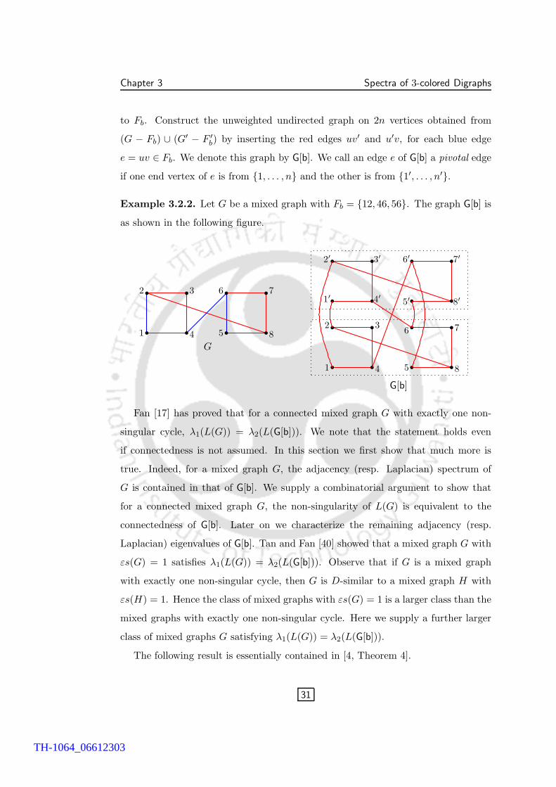
Chapter 3 Spectra of 3-colored Digraphs
to Fb. Construct the unweighted undirected graph on 2n vertices obtained from
(G − Fb) ∪ (G′ − F ′b) by inserting the red edges uv′ and u′v, for each blue edge
e = uv ∈ Fb. We denote this graph by G[b]. We call an edge e of G[b] a pivotal edge
if one end vertex of e is from {1, . . . , n} and the other is from {1′, . . . , n′}.
Example 3.2.2. Let G be a mixed graph with Fb = {12, 46, 56}. The graph G[b] is
as shown in the following figure.
1
2 3
4 5
6 7
8b
b b
b b
b b
b
G
1
2 3
4 5
6 7
8b
b b
b b
b b
b
1′
2′ 3′
4′ 5′
6′ 7′
8′b
b b
b b
b b
b
G[b]
Fan [17] has proved that for a connected mixed graph G with exactly one non-
singular cycle, λ1(L(G)) = λ2(L(G[b])). We note that the statement holds even
if connectedness is not assumed. In this section we first show that much more is
true. Indeed, for a mixed graph G, the adjacency (resp. Laplacian) spectrum of
G is contained in that of G[b]. We supply a combinatorial argument to show that
for a connected mixed graph G, the non-singularity of L(G) is equivalent to the
connectedness of G[b]. Later on we characterize the remaining adjacency (resp.
Laplacian) eigenvalues of G[b]. Tan and Fan [40] showed that a mixed graph G with
εs(G) = 1 satisfies λ1(L(G)) = λ2(L(G[b])). Observe that if G is a mixed graph
with exactly one non-singular cycle, then G is D-similar to a mixed graph H with
εs(H) = 1. Hence the class of mixed graphs with εs(G) = 1 is a larger class than the
mixed graphs with exactly one non-singular cycle. Here we supply a further larger
class of mixed graphs G satisfying λ1(L(G)) = λ2(L(G[b])).
The following result is essentially contained in [4, Theorem 4].
31
TH-1064_06612303
Chapter 3 Spectra of 3-colored Digraphs
Lemma 3.2.3. Let G be a connected mixed graph with Fb 6= ∅. If L(G) is singular,
then G − Fb is disconnected. Furthermore, there is partition V (G) = V1 ∪ V2 such
that E(V1, V2) = Fb.
The following are some crucial observations.
Lemma 3.2.4. Let G be a connected mixed graph and P be a 1-u-path in G. Then
the following statements hold.
(a) If P contains an odd number of blue edges, then we have a 1-u′-path P1u′ and
a 1′-u-path P1′u in G[b].
(b) If P contains an even number of blue edges, then we have a 1-u-path P1u and
a 1′-u′-path P1′u′ in G[b].
Proof. The proof is similar to the proof of Lemma 3.1.5
Next, we give a characterization of the non-singular mixed graphs.
Theorem 3.2.5. Let G be a connected mixed graph. Then L(G) is non-singular if
and only if G[b] is connected.
Proof. Assume that L(G) is non-singular. Then G contains a non-singular cycle,
say C = [1, . . . , k, 1]. As C contains an odd number of blues edges, by Lemma
3.2.4(b), there is 1-1′-path in G[b]. Let u be any vertex in G. Since G is connected,
there is a 1-u-path from 1 to u. Again by Lemma 3.2.4, there is a path from u either
to 1 or to 1′. Moreover, there is also a path from u′ either to 1 or to 1′. Hence G[b]
is connected.
Conversely, suppose that G does not contain a cycle of weight −1. By Lemma
3.2.3, there is a partition V (G) = V1 ∪ V2 such that E(V1, V2) = Fb. Then in G[g]
there cannot be a path from a vertex of V1 to any vertex of V ′1 .
An alternate way to see the converse is the following. Suppose that G[b] is
connected. Take a 1-1′-path P in G[b]. The path P can only contain an odd number
of pivotal edges due to the structure of G[b]. The existence of a pivotal edge ij′ or
i′j in G[b] implies that the edge ij in G has color blue. Hence P describes a 1-1-walk
32
TH-1064_06612303
Chapter 3 Spectra of 3-colored Digraphs
in G containing an odd number of blue edges. Thus there must be a cycle in G
containing an odd number of blue edges, implying that G has a cycle of weight −1.
So L(G) is non-singular.
Definition 3.2.6. Let G be a mixed graph on vertices 1, . . . , n. Recall that Fb
denotes the set of blue edges in G. We define Bb = [cij ] to be the n×n matrix with
cij = cji = 1 if ij ∈ Fb, and 0 otherwise. By Db we denote the diagonal matrix with
i-th diagonal entry equal to the number of blue edges incident with the vertex i in
G.
The proof of the next result follows from the construction of G[b].
Proposition 3.2.7. Let G be a mixed graph. Then
A(G[b]) = I2 ⊗ A(G − Fb) +
[0 11 0
]⊗ Bb,
A(G) = A(G − Fb) − Bb,
L(G[b]) = I2 ⊗ L(G − Fb) + I2 ⊗ Db −[0 11 0
]⊗ Bb,
L(G) = L(G − Fb) + Db + Bb.
Next, we relate the Laplacian (resp. adjacency) spectrum of the mixed graph G
with that of G[b].
Lemma 3.2.8. Let G be a mixed graph and λ be a Laplacian (resp. adjacency)
eigenvalue of G with an eigenvector x. Then λ is a Laplacian (resp. adjacency)
eigenvalue of G[b] with an eigenvector
[x
−x
].
Proof. We prove the statement only for L(G[b]). The proof of the statement for
A(G[b]) is similar. Put y =
[1
−1
]. Observe that
[0 11 0
]y = −y. Hence
L(G[b])(y ⊗ x) = y ⊗ L(G − Fb)x + y ⊗ Dbx −[0 11 0
]y ⊗ Bbx
= y ⊗ [L(G − Fb) + Db + Bb]x= y ⊗ L(G)x, using Proposition 3.2.7= y ⊗ λx= λ(y ⊗ x).
33
TH-1064_06612303
Chapter 3 Spectra of 3-colored Digraphs
So L(G[b])
[x
−x
]= λ
[x
−x
].
The following result whose proof follows immediately from Lemma 3.2.8 is the
main result of this section. This answers the questions raised in the beginning of
this section.
Theorem 3.2.9. Let G be a mixed graph. Then the adjacency (resp. Lapla-
cian) spectrum of the unweighted undirected graph G[b] contains the adjacency (resp.
Laplacian) spectrum of G.
In view of Theorem 3.2.9, we have the following natural question: Does there exist
an unweighted undirected graph whose adjacency (resp. Laplacian) eigenvalues are the
remaining n adjacency (resp. Laplacian) eigenvalues of G[b]?
Definition 3.2.10. Let G be a connected mixed graph. By Gb�r we mean the
unweighted undirected graph obtained from G, changing the color of each blue edge
in G to red.
Using the same notations as in Definition 3.2.6 we observe that
A(Gb�r) = A(G − Fb) + Bb
D(Gb�r) = D(G)
L(Gb�r) = L(G − Fb) + Db − Bb.
�
�
�
�3.2.1
Next, we show that the adjacency (resp. Laplacian) eigenvalues of Gb�r are indeed
the adjacency (resp. Laplacian) eigenvalues of G[b].
Lemma 3.2.11. Let G be a mixed graph and λ be a Laplacian (resp. adjacency)
eigenvalue of Gb�r with an eigenvector x. Then λ is a Laplacian (resp. adjacency)
eigenvalue of G[b] with an eigenvector
[xx
].
Proof. We prove the statement only for L(Gb�r). The proof of the statement for
A(Gb�r) is similar. Put y =
[11
]. Observe that
[0 11 0
]y = y. Hence
L(G[b])(y ⊗ x) = y ⊗ [L(G − Fb) + Db − Bb]x= y ⊗ L(Gb�
r)x, using Proposition 3.2.7 and equation (3.2.1)= y ⊗ λx= λ(y ⊗ x).
34
TH-1064_06612303
Chapter 3 Spectra of 3-colored Digraphs
So L(G[b])
[xx
]= λ
[xx
].
Using Theorem 3.2.9 and Lemma 3.2.11 we obtain the following result which is
one of the main results of this section. This also answers our earlier question.
Theorem 3.2.12. Let G be a connected mixed graph. Then the Laplacian (resp.
adjacency) spectrum of G[b] is the union of the Laplacian (resp. adjacency) spectra
of G and Gb�r.
The second smallest Laplacian eigenvalue λ2(L(G)) of an undirected graph G is
popularly known as the algebraic connectivity of G, denoted by a(G). The following
is an immediate corollary.
Corollary 3.2.13. Let G be a non-singular connected mixed graph. Then a(G[b]) =
min{λ1(L(G)), a(Gb�r)}.
It is natural to ask for a characterization of non-singular mixed graphs G such that
a(G[b]) = λ1(L(G)). Fan[17], Tan and Fan[40] have provided some class of such non-
singular mixed graphs. In the next theorem, we provide a more general class (than
that of Fan, Tan and Fan) of non-singular mixed graphs G with a(G[b]) = λ1(L(G)).
Theorem 3.2.14. Let G be a non-singular connected mixed graph such that a(Gb�r)
has multiplicity k. Let W ⊂ V (G) be such that 0 < |W | ≤ k and that G−W has all
components singular. Then a(G[b]) = λ1(L(G)).
Proof. Let LW and L′W be the principal submatrices of L(G) and L(Gb�
r) corre-
sponding to the graphs G−W and Gb�r−W , respectively. By Theorem 2.3.4, LW is
D-similar to L′W . By interlacing theorem, λ1(L(G)) ≤ λ1(LW ) = λ1(L
′W ) ≤ a(Gb�
r).
Hence a(G[b]) = λ1(L(G)), by Corollary 3.2.13.
Example 3.2.15. Consider G as shown below. Note that the a(Gb�r) has multi-
plicity 2 and G − W is singular, where W = {9, 13}. Thus a(G[b]) = λ1(L(G)).
35
TH-1064_06612303
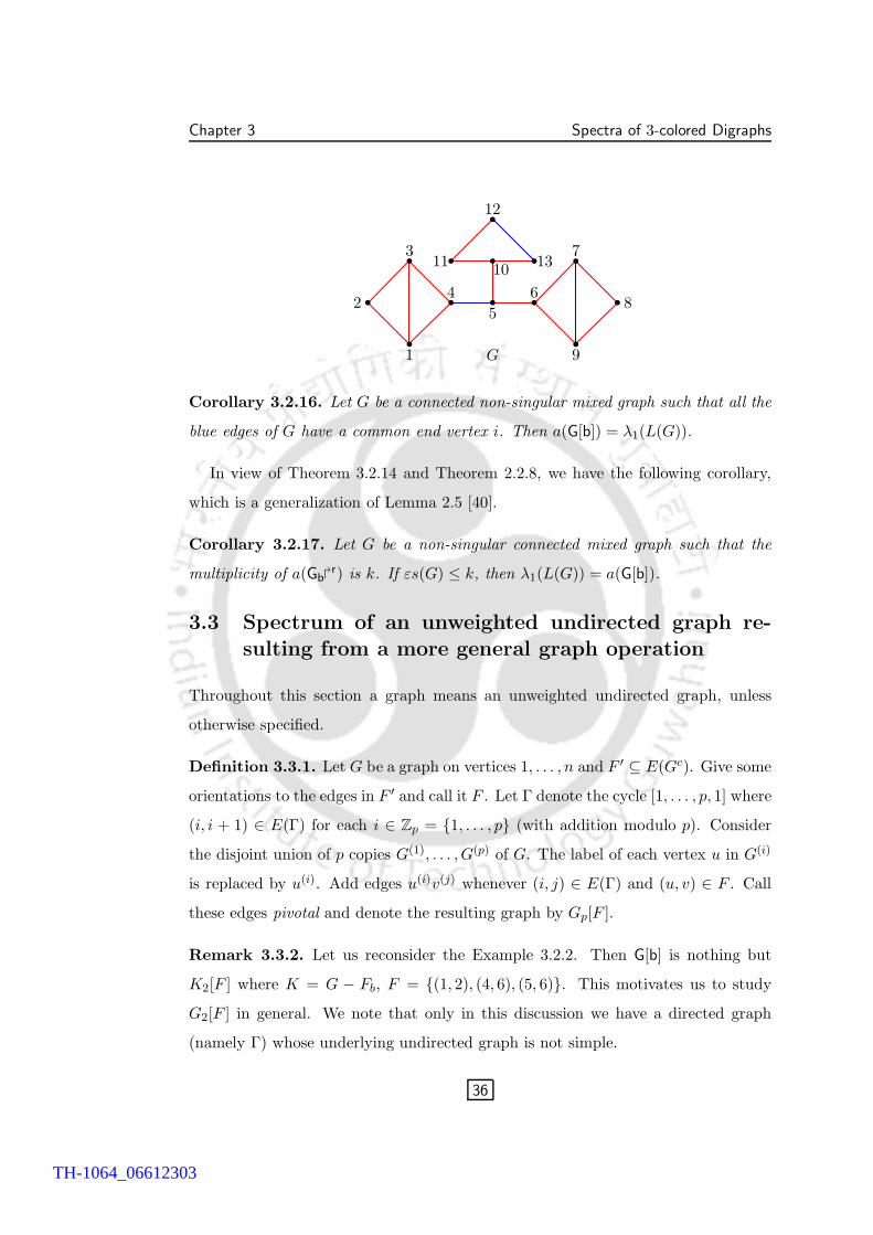
Chapter 3 Spectra of 3-colored Digraphs
b
1
b2
b3
b4
b11
b
5
b
10
b12
b6
b 13
b
9
b7
b 8
G
Corollary 3.2.16. Let G be a connected non-singular mixed graph such that all the
blue edges of G have a common end vertex i. Then a(G[b]) = λ1(L(G)).
In view of Theorem 3.2.14 and Theorem 2.2.8, we have the following corollary,
which is a generalization of Lemma 2.5 [40].
Corollary 3.2.17. Let G be a non-singular connected mixed graph such that the
multiplicity of a(Gb�r) is k. If εs(G) ≤ k, then λ1(L(G)) = a(G[b]).
3.3 Spectrum of an unweighted undirected graph re-
sulting from a more general graph operation
Throughout this section a graph means an unweighted undirected graph, unless
otherwise specified.
Definition 3.3.1. Let G be a graph on vertices 1, . . . , n and F ′ ⊆ E(Gc). Give some
orientations to the edges in F ′ and call it F . Let Γ denote the cycle [1, . . . , p, 1] where
(i, i + 1) ∈ E(Γ) for each i ∈ Zp = {1, . . . , p} (with addition modulo p). Consider
the disjoint union of p copies G(1), . . . , G(p) of G. The label of each vertex u in G(i)
is replaced by u(i). Add edges u(i)v(j) whenever (i, j) ∈ E(Γ) and (u, v) ∈ F . Call
these edges pivotal and denote the resulting graph by Gp[F ].
Remark 3.3.2. Let us reconsider the Example 3.2.2. Then G[b] is nothing but
K2[F ] where K = G − Fb, F = {(1, 2), (4, 6), (5, 6)}. This motivates us to study
G2[F ] in general. We note that only in this discussion we have a directed graph
(namely Γ) whose underlying undirected graph is not simple.
36
TH-1064_06612303
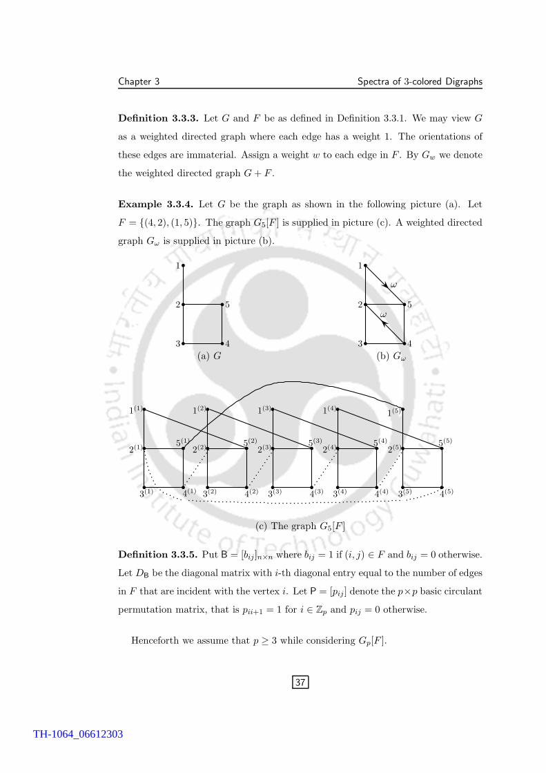
Chapter 3 Spectra of 3-colored Digraphs
Definition 3.3.3. Let G and F be as defined in Definition 3.3.1. We may view G
as a weighted directed graph where each edge has a weight 1. The orientations of
these edges are immaterial. Assign a weight w to each edge in F . By Gw we denote
the weighted directed graph G + F .
Example 3.3.4. Let G be the graph as shown in the following picture (a). Let
F = {(4, 2), (1, 5)}. The graph G5[F ] is supplied in picture (c). A weighted directed
graph Gω is supplied in picture (b).
b
b b
b
b1
2
3 4
5
(a) G
b
b b
b
b1
2
3 4
5
(b) Gω
ω
ω
b
b b
b
b1(1)
2(1)
3(1) 4(1)
5(1)
b
b b
b
b1(2)
2(2)
3(2) 4(2)
5(2)
b
b b
b
b1(3)
2(3)
3(3) 4(3)
5(3)
b
b b
b
b1(4)
2(4)
3(4) 4(4)
5(4)
b
b b
b
b
1(5)
2(5)
3(5) 4(5)
5(5)
(c) The graph G5[F ]
Definition 3.3.5. Put B = [bij]n×n where bij = 1 if (i, j) ∈ F and bij = 0 otherwise.
Let DB be the diagonal matrix with i-th diagonal entry equal to the number of edges
in F that are incident with the vertex i. Let P = [pij ] denote the p×p basic circulant
permutation matrix, that is pii+1 = 1 for i ∈ Zp and pij = 0 otherwise.
Henceforth we assume that p ≥ 3 while considering Gp[F ].
37
TH-1064_06612303
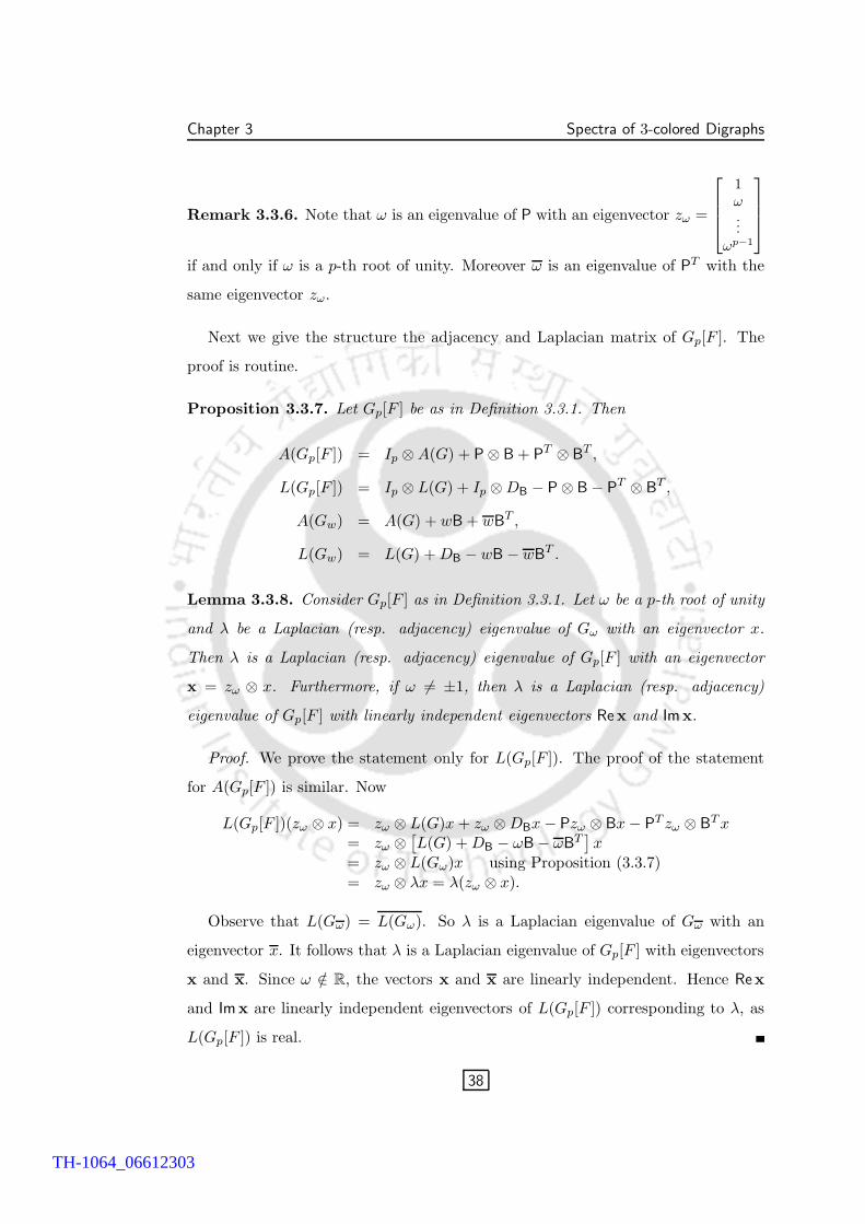
Chapter 3 Spectra of 3-colored Digraphs
Remark 3.3.6. Note that ω is an eigenvalue of P with an eigenvector zω =
1ω...
ωp−1
if and only if ω is a p-th root of unity. Moreover ω is an eigenvalue of PT with the
same eigenvector zω.
Next we give the structure the adjacency and Laplacian matrix of Gp[F ]. The
proof is routine.
Proposition 3.3.7. Let Gp[F ] be as in Definition 3.3.1. Then
A(Gp[F ]) = Ip ⊗ A(G) + P ⊗ B + PT ⊗ BT ,
L(Gp[F ]) = Ip ⊗ L(G) + Ip ⊗ DB − P ⊗ B − PT ⊗ BT ,
A(Gw) = A(G) + wB + wBT ,
L(Gw) = L(G) + DB − wB − wBT .
Lemma 3.3.8. Consider Gp[F ] as in Definition 3.3.1. Let ω be a p-th root of unity
and λ be a Laplacian (resp. adjacency) eigenvalue of Gω with an eigenvector x.
Then λ is a Laplacian (resp. adjacency) eigenvalue of Gp[F ] with an eigenvector
x = zω ⊗ x. Furthermore, if ω 6= ±1, then λ is a Laplacian (resp. adjacency)
eigenvalue of Gp[F ] with linearly independent eigenvectors Rex and Imx.
Proof. We prove the statement only for L(Gp[F ]). The proof of the statement
for A(Gp[F ]) is similar. Now
L(Gp[F ])(zω ⊗ x) = zω ⊗ L(G)x + zω ⊗ DBx − Pzω ⊗ Bx − PT zω ⊗ BT x= zω ⊗
[L(G) + DB − ωB − ωBT
]x
= zω ⊗ L(Gω)x using Proposition (3.3.7)= zω ⊗ λx = λ(zω ⊗ x).
Observe that L(Gω) = L(Gω). So λ is a Laplacian eigenvalue of Gω with an
eigenvector x. It follows that λ is a Laplacian eigenvalue of Gp[F ] with eigenvectors
x and x. Since ω /∈ R, the vectors x and x are linearly independent. Hence Rex
and Imx are linearly independent eigenvectors of L(Gp[F ]) corresponding to λ, as
L(Gp[F ]) is real.
38
TH-1064_06612303
Chapter 3 Spectra of 3-colored Digraphs
The following result whose proof follows immediately from Lemma 3.3.8 is the
main result of this section.
Theorem 3.3.9. Consider Gp[F ] as in Definition 3.3.1. Let ω be a p-th root of
unity such that ωk 6= 1, for 0 < k < p. Then the Laplacian (resp. adjacency)
spectrum of Gp[F ] is the union of the Laplacian (resp. adjacency) spectrum of the
weighted directed graphs Gω1 , . . . , Gωp .
Remark 3.3.10. Note that the Laplacian (resp. adjacency) spectrum of Gω and
Gω are the same. So for each p-th root of unity ω(6= ±1), each Laplacian (resp.
adjacency) eigenvalue of Gω appears at least twice in the Laplacian (resp. adjacency)
spectrum of Gp[F ].
39
TH-1064_06612303
Chapter 4
3-colored digraphs with exactly one non-singular
cycle
In Section 4.1 we describe the structure of 3-colored digraphs containing exactly one
non-singular cycle. We show that given a connected 3-colored digraph G containing
exactly one non-singular cycle, there is a graph H with a(H) = λ1(L(G)). In Sec-
tion 4.2 we establish a monotonicity property on the real and imaginary parts of the
eigenvectors corresponding to λ1(L(G)), which is analogous to Fiedler’s monotonic-
ity Theorem. We describe the sign structure of the real and imaginary parts of the
eigenvectors corresponding to λ1(L(G)). In Section 4.3 we prove that among all non-
singular unicyclic 3-colored digraphs on n vertices, the smallest Laplacian eigenvalue
is minimized by the cycle of weight ±i and length n. The non-singular unicyclic 3-
colored digraphs which maximizes the smallest Laplacian eigenvalue over all such
graphs is discussed in Section 4.4. In Section 4.5 we characterize the non-singular
unicyclic 3-colored digraphs G having λ2(L(G)) = 1.
4.1 Smallest Laplacian eigenvalue
The following lemmas are crucial in describing the structure of a 3-colored digraph
containing exactly one non-singular cycle.
Lemma 4.1.1. Let G be a connected 3-colored digraph containing exactly one non-
singular cycle C. Then the following holds:
(i) If wC = −1, then G is D-similar to DG with all edges red except one edge on C
which is blue.
40
TH-1064_06612303
Chapter 4 3-colored digraphs with exactly one non-singular cycle
(ii) If wC = ±i, then G is D-similar to DG with all edges red except one edge on
C which is green.
Proof. Let e be an edge on the cycle C in G. Take G′ = G−e. By Lemma 2.1.11,
G′ is singular and by Lemma 2.3.4, each edge in DG′ has color red. Consider DG for
this D. Note that all the edges in DG except the edge corresponding to e have color
red. Since weight of a cycle does not change in D-similar copies, we see that weight
of the edge corresponding to e in DG is wC or wC . Hence the result holds.
Lemma 4.1.2. Let G be a 3-colored digraph containing exactly one non-singular
cycle C. Then the subgraph induced by C is C itself.
Proof. Consider C = [1, . . . ,m, 1]. If possible, suppose that C has a chord joining
the vertices i and j with 1 ≤ i < j ≤ m. Take the cycles C1 = [1, i, j . . . ,m, 1] and
C2 = [i, i+1, . . . , j, i]. Note that wC1wC2
= wC 6= 1, which implies one of C1 and C2
has weight other than 1. Hence G contains at least two non-singular cycles, which
is a contradiction.
Lemma 4.1.3. Let G be a connected 3-colored digraph containing exactly one non-
singular cycle C. Let u be a vertex of G not on C. Then there is a vertex v on the
cycle C such that G−v is disconnected with at least two components, one containing
u and another containing the remaining vertices of C.
Proof. In view of Lemma 4.1.1, we assume that all the edges of G have color
red except an edge e on the cycle C. Since G is connected, let v be a vertex in the
cycle for which the distance d(v, u) is minimum. Let Puv be a shortest u-v-path in
G. Then the vertex v is on every u-w-path, for each vertex w in C. If not, suppose
G contains a u-w-path, say Puw which does not contain v, for some vertex w in C.
Let Pvw(e) be the v-w-path on the cycle C containing the edge e. Take the cycle
C ′ = Puv + Pvw(e) + Puw. Note that wC′ 6= 1. So the cycle C ′ is non-singular, by
Theorem 2.1.11, which is a contradiction. Hence G− v is disconnected with at least
two components, one containing u and another containing the remaining vertices of
C.
41
TH-1064_06612303
Chapter 4 3-colored digraphs with exactly one non-singular cycle
Next corollary follows immediately, which generalizes [17, Lemma 2.1].
Corollary 4.1.4. Let G be a connected 3-colored digraph with exactly one non-
singular cycle. If G has no cut vertex, then G is exactly the non-singular cycle.
Definition 4.1.5. Let G be a connected 3-colored digraph containing exactly one
non-singular cycle C and let u be a vertex on C. In view of Lemma 4.1.3, let H be
the component of G − u, which contains the remaining vertices of C. Notice that if
G − u is connected, then H = G − u. We define Gu to be the graph G − V (H).
Next lemma characterizes the structure of connected 3-colored digraphs contain-
ing exactly one non-singular cycle.
Lemma 4.1.6. Let G be a 3-colored connected digraph on vertices 1, · · · , n. Then
the following two statements are equivalent.
(a) G has exactly one non-singular cycle C = [1, . . . ,m, 1].
(b) G is obtained from a non-singular cycle C = [1, . . . ,m, 1] by appending a sin-
gular connected graph Gi to the vertex i of C while identifying a vertex of Gi
with i, for each i = 1, . . . ,m.
Proof. (a) ⇒ (b). Assume that G has exactly one non-singular cycle C =
[1, . . . ,m, 1]. By Lemma 4.1.2, the subgraph induced by C is C itself. In view of
Lemma 4.1.3, for each i = 1, . . . ,m, let Gi = G−V (Hi), where Hi is the component
of the graph containing the remaining vertices of C. As Gi does not contain a non-
singular cycle, Gi is singular, for each i = 1, . . . ,m. Hence the result holds. (b)⇒(a)
is trivial.
Remark 4.1.7. Let G be a connected 3-colored digraph with exactly one non-
singular cycle C = [1, . . . ,m, 1]. In view of Lemma 4.1.1 and Lemma 4.1.6, DG is
as in figure 4.1 or figure 4.2, if wC = ±i or wC = −1, respectively. We denote the
graph in Figure 4.1, by Gg and the graph in Figure 4.2, by Gb.
42
TH-1064_06612303
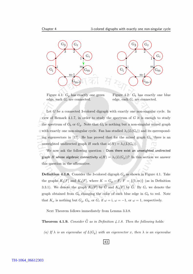
Chapter 4 3-colored digraphs with exactly one non-singular cycle
G3
i
G2
23G1
1
Gm-1
Gmm
Gim-1
b
b
b
b
b
b
b
b
Figure 4.1: Gg has exactly one greenedge, each Gi are connected.
G3
i
G2
23G1
1
Gm-1
Gmm
Gim-1
b
b
b
b
b
b
b
b
Figure 4.2: Gb has exactly one blueedge, each Gi are connected.
Let G be a connected 3-colored digraph with exactly one non-singular cycle. In
view of Remark 4.1.7, in order to study the spectrum of G it is enough to study
the spectrum of Gb or Gg. Note that Gb is nothing but a non-singular mixed graph
with exactly one non-singular cycle. Fan has studied λ1(L(Gb)) and its correspond-
ing eigenvectors in [17]. He has proved that for the mixed graph Gb, there is an
unweighted undirected graph H such that a(H) = λ1(L(Gb)).
We now ask the following question : Does there exist an unweighted undirected
graph H whose algebraic connectivity a(H) = λ1(L(Gg))? In this section we answer
this question in the affirmative.
Definition 4.1.8. Consider the 3-colored digraph Gg as shown in Figure 4.1. Take
the graphs K2[F ] and K4[F ], where K = Gg − F , F = {(1,m)} (as in Definition
3.3.1). We denote the graph K2[F ] by G and K4[F ] by G. By Gr we denote the
graph obtained from Gb changing the color of each blue edge in Gb to red. Note
that Kω is nothing but Gg, Gb, or Gr if ω = i, ω = −1, or ω = 1, respectively.
Next Theorem follows immediately from Lemma 3.3.8.
Theorem 4.1.9. Consider G as in Definition 4.1.8. Then the following holds:
(a) If λ is an eigenvalue of L(Gg) with an eigenvector x, then λ is an eigenvalue
43
TH-1064_06612303
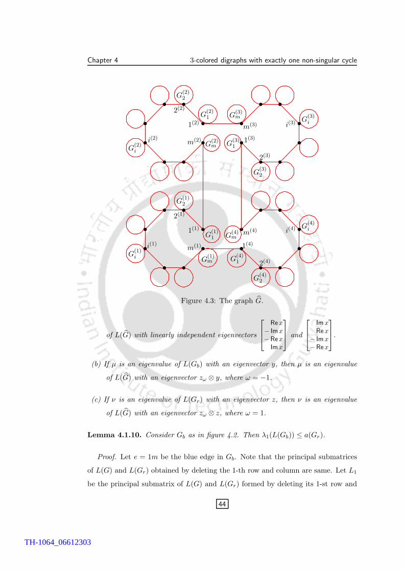
Chapter 4 3-colored digraphs with exactly one non-singular cycle
i(1)
G(1)2
2(1)
G(1)1
1(1)
G(1)m
m(1)
G(1)i
i(2)
G(2)2
2(2)
G(2)1
1(2)
G(2)m
m(2)
G(2)i
1(3)G
(3)1
G(3)2
2(3)
G(3)ii(3)
G(3)m
m(3)
b
b
b
b
b
b
b
b
b
b
b
b
b
b
b
b G(4)ii(4)m(4)
G(4)m
1(4)
G(4)1
G(4)2
2(4)
b
b
b
b
b
b
b
b
b
b
b
b
b
b
b
b
Figure 4.3: The graph G.
of L(G) with linearly independent eigenvectors
Rex− Imx−Rex
Im x
and
Im xRe x
− Im x−Rex
.
(b) If µ is an eigenvalue of L(Gb) with an eigenvector y, then µ is an eigenvalue
of L(G) with an eigenvector zω ⊗ y, where ω = −1.
(c) If ν is an eigenvalue of L(Gr) with an eigenvector z, then ν is an eigenvalue
of L(G) with an eigenvector zω ⊗ z, where ω = 1.
Lemma 4.1.10. Consider Gb as in figure 4.2. Then λ1(L(Gb)) ≤ a(Gr).
Proof. Let e = 1m be the blue edge in Gb. Note that the principal submatrices
of L(G) and L(Gr) obtained by deleting the 1-th row and column are same. Let L1
be the principal submatrix of L(G) and L(Gr) formed by deleting its 1-st row and
44
TH-1064_06612303
Chapter 4 3-colored digraphs with exactly one non-singular cycle
column. Then by interlacing theorem we have λ1(L(Gb)) ≤ λ1(L1) ≤ a(Gr). Hence
λ1(L(Gb)) ≤ a(Gr).
Definition 4.1.11. Let G be a 3-colored digraph. We call an eigenvector corre-
sponding to λ1(L(G)) a first eigenvector of G.
Next Lemma follows immediately using Lemma 3.3.8 and Lemma 4.1.10.
Lemma 4.1.12. [17, Lemma 2.4] Consider Gb as in figure 4.2 and let x be a first
eigenvector of Gb. Then a(G) = λ1(L(Gb)) and
[x
−x
]is a Fiedler vector of G.
Remark 4.1.13. Let G be a connected 3-colored digraph with exactly one non-
singular cycle C. Assume that C contains an even number of green edges. If x is a
first eigenvector of G, then
[Re D−1y
−ReD−1y
],
[ImD−1y
− ImD−1y
]are Fiedler vectors of G, for
some diagonal matrix D with diagonal entries ±1,±i.
Lemma 4.1.14. [6, Theorem 12] Let G be a connected graph and Y be a Fiedler
vector. Let S = C(G,Y ). Suppose S lies in the block B. Then 1 ≤ |S| ≤ NB + 1.
Next Lemma says non-negativity of the first eigenvector of Gb on the cycle.
Lemma 4.1.15. Consider the mixed graph Gb as in figure 4.2. Then Gb is D-
similar to a mixed graph H such that a first eigenvector of H is non-negative on the
vertices of the non-singular cycle in H.
Proof. Proof is similar to that of [22, Theorem 2.9].
Lemma 4.1.16. Consider Gg and Gb as in figure 4.1 and figure 4.2, respectively.
Then λ1(L(Gg)) ≤ λ1(L(Gb)).
Proof. In view of Lemma 4.1.15, let x be a first eigenvector of Gb such that x is
non-negative on the vertices of the cycle containing the blue edge e = ij. Then
λ1(L(Gb)) = x∗L(Gb)x =∑
(u,v)∈E(Gb−e)
|xu − xv|2 + (xi + xj)2
≥∑
(u,v)∈E(Gb−e)
|xu − xv|2 + |xi + ixj |2
≥ min x∗L(Gg)x ≥ λ1(L(Gg)).
45
TH-1064_06612303
Chapter 4 3-colored digraphs with exactly one non-singular cycle
Theorem 4.1.17. Consider Gg as in figure 4.1. Let x be a first eigenvector of Gg.
Then a(G) = λ1(L(Gg)) and x =
Re x− Imx−Rex
Im x
, y =
Im xRe x
− Imx−Rex
are linearly independent
Fiedler vectors.
Proof. Note that λ1(L(Gg)) ≤ λ1(L(Gb)) ≤ a(Gr), by Lemma 4.1.10 and Lemma
4.1.16. Hence a(G) = λ1(L(Gg)), and x, y are linearly independent Fiedler vectors
of G, by Theorem 4.1.9(a).
Next corollary follows immediately from Lemma 4.1.1 and Theorem 4.1.17.
Corollary 4.1.18. Let G be a 3-colored digraph containing exactly one non-singular
cycle C. Assume that C contains an odd number of green edges. If x is a first
eigenvector of G, then
ReD−1x− ImD−1x−ReD−1x
ImD−1x
and
Im D−1xReD−1x
− ImD−1x−ReD−1x
are Fiedler vectors of G, for
some diagonal matrix D with the diagonal entries ±1,±i.
4.2 First eigenvectors of Gg
Fan [17] has studied the structure of the first eigenvectors of Gb. In this section,
we describe the structure of the real and imaginary parts of first eigenvectors of Gg.
Finally, we prove that multiplicity of λ1(L(Gg)) is one.
Proposition 4.2.1. [25, Fiedler’s monotonicity theorem] Let G be a connected graph
and y be a Fiedler vector of G. Then exactly one of the following cases occurs:
Case A: There is exactly one block B in G which contains both positively and
negatively valuated vertices (with respect to y). Every other block has either vertices
with positive valuation only, or vertices with negative valuation only, or vertices with
zero valuation only. Every pure path P which starts at a vertex i of B and contains
no other vertex of B has the property that the valuations at points of articulation
contained in P form either an increasing, or decreasing, or a zero sequence along
this path according to whether y(i) > 0, y(i) < 0 or y(i) = 0; in the last case all
vertices in P have valuation zero.
46
TH-1064_06612303
Chapter 4 3-colored digraphs with exactly one non-singular cycle
Case B: No block of G contains both positively and negatively valuated vertices
(with respect to y). In this case, there exists a unique vertex k which has valuation
zero and is adjacent to a vertex with non-zero valuation. This vertex k is a point
of articulation. Each block with respect to y contains (with exception of k) either
vertices with positive valuation only, vertices with negative valuation only, or vertices
with zero valuation only. Every pure path P which starts at k has the property that
the valuations at its points of articulation either increase, and then all valuations of
vertices on P are (with exception of k) positive, or decrease, and then all valuations
of vertices on P are (with exception of k) negative, or all valuations of vertices on P
are zero. Every path containing both positively and negatively valued vertices passes
through k.
Theorem 4.2.2. Consider Gg as in figure 4.1. Let C = [1, . . . ,m, 1] be the non-
singular cycle with the green edge e = (1,m). Let x be a first eigenvector of Gg.
Then the following holds:
(a) The cycle C contains a nonzero valuated vertex (with respect to x) and G
satisfies Case A of Proposition 4.2.1.
(b) Each block B of Gg other than C has either vertices of valuations with positive
real part (resp. imaginary part) only, or vertices with negative real part (resp.
imaginary part) only, or vertices with zero real part (resp. imaginary part)
only.
(c) Every path P which starts at a vertex v of C and contains no other vertex
of C has the property that the real part (resp. imaginary part) of the valua-
tions at the points of articulation contained in P form either an increasing,
decreasing, or zero sequence along this path according to whether Re x(v) > 0
(resp. Imx(v) > 0), Rex(v) < 0 (resp. Im x(v) < 0), or Rex(v) = 0 (resp.
Imx(v) = 0), respectively. In the last case all vertices in P have real part
(resp. imaginary part) zero.
Proof. (a) If possible, suppose that the valuations of x at the vertices of C are
all zero. Let P (i) denote the 1(i)-m(i)-path in G corresponding to the 1-m-path in
47
TH-1064_06612303
Chapter 4 3-colored digraphs with exactly one non-singular cycle
Gg − e, for i = 1, 2, 3, 4. Take the cycle
C = P (1) + 1(1)m(2) + P (2) + 1(2)m(3) + P (3) + 1(3)m(4) + P (4) + 1(4)m(1).
in G. Note that x (as in Theorem 4.1.17) is a Fiedler vector of G. Thus valuations
of x at the vertices of C are all zero.
Case 1: If G satisfies Case A of Proposition 4.2.1 with respect to x, then there
exist a single block B0 in G containing both positively and negatively valuated
vertices and each other block has either vertices with positive valuation, or negative
valuation, or vertices zero valuations only. Clearly C can not be the block B0. So
B0 must be be contained in some G(i)k (where Gk is as in Definition 4.1.5), for some
k with 1 ≤ k ≤ m. Thus G has at least four blocks containing both positively and
negatively valuated vertices (with respect to x), which is a contradiction.
Case 2: If G satisfies Case B of Proposition 4.2.1 with respect to x, then there
exist a unique vertex ui in G such that x(u) = 0 and u(i) is adjacent to a vertex
w(j) with x(w(j)) 6= 0, for some i, j with 1 ≤ i, j ≤ 4. So w(j) can not be a vertex
in C. Thus w(j) must be contained in G(j)k , for some k with 1 ≤ k ≤ m. From the
structure of G and Gg it follows that i = j, that is, u(i) is a vertex in G(j), where
G(j) is as in Definition 4.1.8. Thus x(u(i)) = 0, x(w(i)) 6= 0, and u(i) is adjacent to
w(i) in G, for i = 1, 2, 3, 4, which is contradiction. Hence the cycle C contains at
least one nonzero valuated vertex (with respect to x).
To prove the second part of (a), let x(j) 6= 0, for some vertex j in C. Thus
from the structure of G and x, it follows that C contains both positively and nega-
tively valuated vertices (with respect to x). Hence the graph G satisfies Case A of
Proposition 4.2.1, with respect to x.
(b) Let B 6= C be a block of Gg. Then B is contained in some Gi, for i = 1, . . . ,m.
Note that the blocks B(i) in G corresponding to B, for i = 1, 2, 3, 4 contains vertices
either with positive valuation only, vertices with negative valuation only, or vertices
with zero valuation only (with respect to x), by part (a). Hence with respect to x,
the block B contains vertices with positive real part (resp. imaginary part) only or
vertices with negative real part (resp. imaginary part) only or vertices with zero
48
TH-1064_06612303
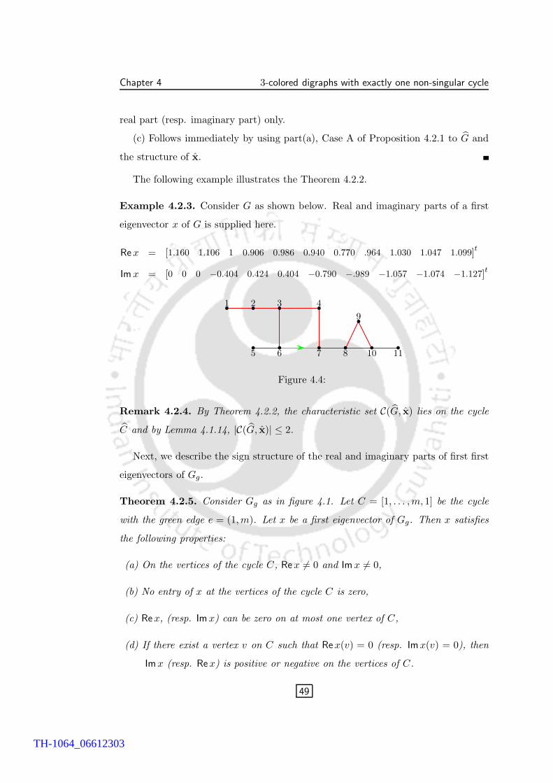
Chapter 4 3-colored digraphs with exactly one non-singular cycle
real part (resp. imaginary part) only.
(c) Follows immediately by using part(a), Case A of Proposition 4.2.1 to G and
the structure of x.
The following example illustrates the Theorem 4.2.2.
Example 4.2.3. Consider G as shown below. Real and imaginary parts of a first
eigenvector x of G is supplied here.
Rex = [1.160 1.106 1 0.906 0.986 0.940 0.770 .964 1.030 1.047 1.099]t
Im x = [0 0 0 −0.404 0.424 0.404 −0.790 −.989 −1.057 −1.074 −1.127]t
1 2 3 4
5 6 7 8
9
10 11b
b b
b
bb
b b b
b
b
Figure 4.4:
Remark 4.2.4. By Theorem 4.2.2, the characteristic set C(G, x) lies on the cycle
C and by Lemma 4.1.14, |C(G, x)| ≤ 2.
Next, we describe the sign structure of the real and imaginary parts of first first
eigenvectors of Gg.
Theorem 4.2.5. Consider Gg as in figure 4.1. Let C = [1, . . . ,m, 1] be the cycle
with the green edge e = (1,m). Let x be a first eigenvector of Gg. Then x satisfies
the following properties:
(a) On the vertices of the cycle C, Re x 6= 0 and Im x 6= 0,
(b) No entry of x at the vertices of the cycle C is zero,
(c) Rex, (resp. Im x) can be zero on at most one vertex of C,
(d) If there exist a vertex v on C such that Rex(v) = 0 (resp. Imx(v) = 0), then
Imx (resp. Rex) is positive or negative on the vertices of C.
49
TH-1064_06612303
Chapter 4 3-colored digraphs with exactly one non-singular cycle
(e) If there exist vertices u and v on C such that Re x(u)Re x(v) < 0 (resp.
Imx(u) Im x(v) < 0), then Imx (resp. Rex) is positive or negative on the
vertices of C,
(f) Let Rex(1)Re x(m) < 0 (resp. Imx(1) Im x(m) < 0). Then Imx is either
positive or negative, according as Rex(1) is negative or positive.
(g) If Re x(1)Re x(m) > 0 (resp. Imx(1) Im x(m) > 0), then Rex (resp. Im x) is
either positive or negative, according as Rex(1) (resp. Im x(1)) is positive or
negative, respectively.
Proof. Consider the graph G corresponding to Gg as in Definition 4.1.8. Note
that x (as in Theorem 4.1.17) is a Fiedler vector of G. For vertices y, z on C, let
P(i)yz denotes the y(i)-z(i)-path in G corresponding to the y-z-path in Gg − e, for
i = 1, . . . , 4.
(a) If possible, suppose that Re x = 0 on the vertices of C. By Theorem 4.2.2, x
is non-zero on C. Let Imx(u) 6= 0, for some vertex u on C such that length of the
m-u-path in Gg−e is shortest. Observe that x(u(i)) 6= 0, for i = 2, 4 and x(j(i)) = 0,
on every vertex j of C, for i = 1, 3. Thus the paths P(2)mu + 1(1)m(2), P
(2)u1 + 1(2)m(3)
and P(4)mu + 1(3)m(4) in G contains one characteristic vertex of G each, which is a
contradiction to |C(G, x)| ≤ 2. Similarly we can prove that Im x 6= 0 on C.
(b) If possible, let u be a vertex on the cycle C such that x(u) = 0. Then
Re x(u) = 0, Im x(u) = 0. In view of part(a), without loss of generality, let w be a
vertex on C such that Rex(w) 6= 0. Thus x(u(i)) = 0, x(w(i)) 6= 0, for i = 1, 3 and
x(u(2)) = 0 = x(u(4)). Hence if w lies on the 1-u-path in Gg − e, then the paths
P(1)u1 + 1(1)m(2) + P
(2)mu and P
(3)uw contains at least three characteristic vertices of G,
which is a contradiction. Similarly if w lies on the m-u-path in Gg − e, we get a
contradiction.
(c) If possible, let u and v be two vertices on C such that Rex(u) = 0 = Rex(v).
By part(b), Imx(u) 6= 0 and Imx(v) 6= 0, with v is on the u-1-path in Gg − e. Then
the paths
P(1)v1 + 1(1)m(2) + P
(2)m1 + 1(2)m(3) + P (3)
mu and P(3)v1 + 1(3)m(4) + P (4)
mu
50
TH-1064_06612303
Chapter 4 3-colored digraphs with exactly one non-singular cycle
contains at least three characteristic vertices of G, which is a contradiction.
Similarly we can prove for Im x.
(d) Let v be a vertex on C such that Re x(v) = 0. If possible, let Imx(w) = 0,
for some vertex w on C. By part(b), Im x(v) 6= 0, Rex(w) 6= 0. So x(v(i)) 6= 0
& x(w(i)) = 0 for i = 2, 4 and x(v(i)) = 0 & x(w(i)) 6= 0, for i = 1, 3. Thus
|C(G, x)| > 2, which is impossible. Similarity, if Im x(i) Im x(j) < 0 for some vertex
i, j on C, we see that |C(G, x)| > 2, which is contradiction.
(e) Suppose that Re x(u)Re x(v) < 0, for some vertices u, v on the cycle C.
Then x(u(i))x(v(i)) < 0, for i = 1, 3. Thus the paths P(i)uv , for i = 1, 3 contains at
least two characteristic elements of G. Hence the result follows from the fact that
|C(G, x)| ≤ 2.
(f) Proof follows with similar argument.
(g) Suppose that Rex(1)Re x(m) > 0 and Re x(1) > 0. Then the paths 1(1)m(2) +
P(2)1m + 1(2)m(3) and 1(3)m(4) + P
(4)1m + 1(4)m(1) contains at least two characteristic
elements of G. Hence the result follows from the fact that |C(G, x)| ≤ 2.
Next, we prove the non-negativity of the real and imaginary parts on the non-
singular cycle of the first eigenvectors of Gg.
Theorem 4.2.6. Consider Gg as in figure 4.1. Then Gg is D-similar to a 3-colored
digraph H, such that a first eigenvector of H has non-negative real and imaginary
parts on the vertices of the non-singular cycle in H.
Proof. Let x be a first eigenvector of Gg.
If Rex ≥ 0, Imx ≤ 0 on the vertices of C, then we take D = −iIn. If Rex ≤ 0,
Im x ≥ 0 on the vertices of C, then we take D = iIn. In these cases D∗x is non-
negative on the non-singular cycle of DGg.
First we assume that Im x is not non-negative on C. Let u, v be two vertices on
C, such that Im x(u) > 0 and Im x(v) < 0 with 1 ≤ u < v ≤ m. By Lemma 4.2.5(e),
Re x is either positive or negative on C. Without loss of generality suppose that
Re x > 0 on C.
case 1: If Imx(i) 6= 0 for i = 1, . . . ,m, then the u-v-path in Gg − e has an
51
TH-1064_06612303
Chapter 4 3-colored digraphs with exactly one non-singular cycle
edge f joining vertices i0, i0 + 1 with Imx(i0) > 0 and Im x(i0 + 1) < 0. Since
|C(G, x)| ≤ 2, we see that Im x(j) > 0 for each j = 1, . . . , i0 and Im x(j) < 0 for each
j = i0 +1, . . . ,m. Let G1 and G2 be the two components of Gb−f −e, such that G1
contains the vertex 1 and G2 contains the vertex m. Take D = −iI|V (G2)| ⊕ I|V (G1)|.
Then ReD∗x and ImD∗x are nonnegative on the vertices of C, and D∗x is a first
eigenvector of DGg with the green edge f .
case 2: If Imx(i) = 0, for some vertex i on C. Let f be the edge on C, joining the
vertices i0, i0 +1. Since |C(G, x)| ≤ 2, we see that Imx(j) 6= 0, for each vertex j 6= i0
on C. Moreover, Imx(j) > 0 for each j = 1, . . . , i0 − 1 and Imx(j) < 0 for each
j = i0 +1, . . . ,m. Let G1 and G2 be the two components of Gb−f −e, such that G1
contains the vertex 1 and G2 contains the vertex m. Take D = −iI|V (G2)| ⊕ I|V (G1)|.
Then ReD∗x and ImD∗x are non-negative on the vertices of C, and D∗x is a first
eigenvector of DGg with the green edge f . Rest of the proof follows with similar
argument.
Next, we prove that λ1(L(Gg)) has multiplicity one.
Theorem 4.2.7. Consider Gg as in figure 4.1. Let C = [1, . . . ,m, 1] be the cycle in
Gg with the green edge e = (1,m). Then multiplicity of λ1(L(Gg)) is one.
Proof. Proof follows immediately from Theorem 4.2.5(a).
Next, we discuss the multiplicity of λ1(L(Gb)).
Remark 4.2.8. Consider Gb as in figure 4.2 and take G. Let x be a first eigenvector
of Gb. In view of Lemma 4.1.12 and the structure of G, we see that there exist a
vertex u on the non-singular cycle in Gb such that x(u) 6= 0.
The following result is a generalization of [22, Corollary 2.8].
Lemma 4.2.9. Consider Gb as in figure 4.2. Let x be a first eigenvector of Gb. Then
there exist at most one vertex i on the non-singular cycle C such that x(i) = 0.
Proof. Let C = [1, . . . ,m, 1] and e = 1m be the blue edge. If possible, suppose
that there exist two vertices u and v with u < v on C such that x(u) = x(v) = 0. By
52
TH-1064_06612303
Chapter 4 3-colored digraphs with exactly one non-singular cycle
Remark 4.2.8, x(w) 6= 0, for some vertex w on C. If w is on the u-v-path in Gb − e
path, then by Lemma 4.1.12, G has at least four characteristic vertices, which is not
possible. For vertices y, z on C, let P(i)yz denotes the y(i)-z(i)-path in G corresponding
to the y-z-path in Gb − e, for i = 1, 2. If w is not on u-v-path in Gb − e, then the
paths P(1)u1 + 1(1)m(2) + P
(2)mv and P
(1)vm + m(1)1(2) + P
(2)1u in G contains at least two
characteristic vertex each, which is a contradiction. Hence the result holds.
In [22], the authors proved that multiplicity of λ1(L(Gb) is at most two for Gb is
unicyclic. Here Gb is not necessarily unicyclic. Hence the following result generalizes
[22, Theorem 2.14].
Lemma 4.2.10. Consider Gb as in figure 4.2. Then λ1(L(Gb)) has multiplicity at
most two.
Proof. Proof is similar to that of [22, Theorem 2.14] using Lemma 4.2.9.
4.3 Minimizing the smallest Laplacian eigenvalue over
unicyclic 3-colored digraphs
In this section we consider the non-singular unicyclic 3-colored digraphs. In view
of Lemma 4.1.1, throughout this section all our non-singular unicyclic 3-colored
digraphs have all edges red except one blue or green edge on the cycle. Fan [18]
has obtained the non-singular unicyclic mixed graphs on n vertices with a fixed
girth, which minimizes the smallest Laplacian eigenvalue over all such graphs. The
unique graph which minimizes the smallest Laplacian eigenvalue over all non-singular
unicyclic mixed graphs on n vertices was determined in [22].
We ask the following question: Does there exist a unique non-singular unicyclic
3-colored digraph on n vertices, which minimizes the smallest Laplacian eigenvalue over
all such graphs? In this section we answer this question in the affirmative.
Next lemma is an immediate application of the interlacing Theorem [32].
Lemma 4.3.1. Let G be a 3-colored digraph and let G′ be the graph obtained from
G by adding a pendent vertex. Then λ1(L(G′)) ≤ λ1(L(G)).
53
TH-1064_06612303
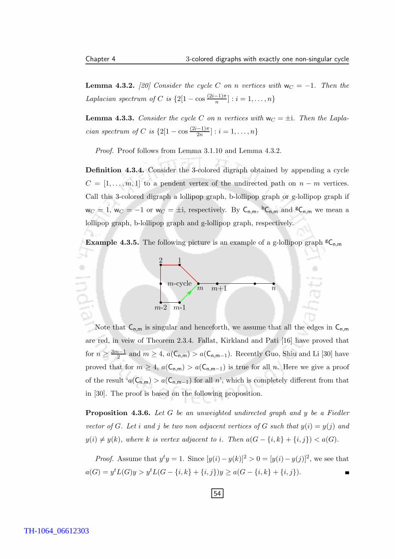
Chapter 4 3-colored digraphs with exactly one non-singular cycle
Lemma 4.3.2. [20] Consider the cycle C on n vertices with wC = −1. Then the
Laplacian spectrum of C is {2[1 − cos (2i−1)πn
] : i = 1, . . . , n}
Lemma 4.3.3. Consider the cycle C on n vertices with wC = ±i. Then the Lapla-
cian spectrum of C is {2[1 − cos (2i−1)π2n
] : i = 1, . . . , n}
Proof. Proof follows from Lemma 3.1.10 and Lemma 4.3.2.
Definition 4.3.4. Consider the 3-colored digraph obtained by appending a cycle
C = [1, . . . ,m, 1] to a pendent vertex of the undirected path on n − m vertices.
Call this 3-colored digraph a lollipop graph, b-lollipop graph or g-lollipop graph if
wC = 1, wC = −1 or wC = ±i, respectively. By Cn,m, bCn,m and gCn,m we mean a
lollipop graph, b-lollipop graph and g-lollipop graph, respectively.
Example 4.3.5. The following picture is an example of a g-lollipop graph gCn,m
b
b b
b
b
b bb
b
bm-cycle
12
m m+1 n
m-1m-2
Note that Cn,m is singular and henceforth, we assume that all the edges in Cn,m
are red, in veiw of Theorem 2.3.4. Fallat, Kirkland and Pati [16] have proved that
for n ≥ 3m−12 and m ≥ 4, a(Cn,m) > a(Cn,m−1). Recently Guo, Shiu and Li [30] have
proved that for m ≥ 4, a(Cn,m) > a(Cn,m−1) is true for all n. Here we give a proof
of the result ‘a(Cn,m) > a(Cn,m−1) for all n’, which is completely different from that
in [30]. The proof is based on the following proposition.
Proposition 4.3.6. Let G be an unweighted undirected graph and y be a Fiedler
vector of G. Let i and j be two non adjacent vertices of G such that y(i) = y(j) and
y(i) 6= y(k), where k is vertex adjacent to i. Then a(G − {i, k} + {i, j}) < a(G).
Proof. Assume that yty = 1. Since [y(i)− y(k)]2 > 0 = [y(i)− y(j)]2, we see that
a(G) = ytL(G)y > ytL(G − {i, k} + {i, j})y ≥ a(G − {i, k} + {i, j}).
54
TH-1064_06612303
Chapter 4 3-colored digraphs with exactly one non-singular cycle
Definition 4.3.7. Let G be a weighted directed graph and let x be an eigenvector
of L(G) corresponding to an eigenvalue λ. By eigen-condition at a vertex i, we mean
the following equation.
(di − λ)x(i) =∑
(i,v)∈E(G)
wivx(v) +∑
(w,i)∈E(G)
wwix(w)
Lemma 4.3.8. [30, Theorem 2.11] Let Cn,m be the lollipop graph on n vertices with
a girth m. Then a(Cn,m−1) < a(Cn,m), for m ≥ 4.
Proof. First we prove the result for m = n. Note that Cn,n is just the cycle
Cn of length n. It is well known that a(Cn) = 2(1 − cos 2πn
) and a vector y ∈ Rn
satisfying y(i) = cos (i−1)2π
n, for i = 1 . . . , n is a Fiedler vector of C − n. Note that
[y(1) − y(n)]2 > 0 = [y(2) − y(n)]2. It follows that for n ≥ 4,
a(Cn) = yTL(Cn,n)y > yT L(Cn,n−1)y ≥ a(Cn,n−1).�
�
�
�4.3.1
Let 4 ≤ m ≤ n − 1 and y be a fiedler vector of Cn,m. If possible, suppose
that y(n) = 0. Then by the eigen-condition at the vertices n, n − 1, . . . ,m + 1,
we see that y(n) = y(n − 1) = · · · = y(m) = 0. In that case, a(Cn,m) is an
eigenvalue of the cycle Cm of length m with an eigenvector [y(1), · · · , y(m)]t. Thus
a(Cn,m) ≥ a(Cm) = 2(1 − cos 2πm
). Note that by Lemma 4.3.1, a(Cn,m) ≤ a(Cm+1,m).
Hence
a(Cn,m) ≤ a(Cm+1,m) < a(Cm+1) = 2(1 − cos2π
m + 1), using equation 4.3.1,
which implies a(Cn,m) < 2(1 − cos 2πm
), a contradiction. So y(n) 6= 0 and hence
a(Cn,m) has multiplicity one.
Let z ∈ Rn be a vector such that z(i) = y(m − i), for i = 1, . . . ,m − 1 and
z(i) = y(i), for i = m,m + 1, . . . , n. Observe that z is also an eigenvector of Cn,m
corresponding to the eigenvalue a(Cn,m). Thus y = z and hence y(1) = y(m − 1).
Since y(n) 6= 0, we assume that y(n) > 0.
If y(m) > 0, then the characteristic set of Cn,m lies on the cycle. In that case
y(1) 6= y(m), otherwise using eigen-condition at the vertex m of Cn,m we have
y(m) − y(m + 1) = a(Cn,m)y(m) > 0, which is a contradiction to Proposition 4.2.1.
55
TH-1064_06612303
Chapter 4 3-colored digraphs with exactly one non-singular cycle
If y(m) < 0, then the characteristic set of Cn,m lies on the path joining the vertices
m and n. In that case y(1) 6= y(m), otherwise using eigencondition at the vertices
of the cycle we see that y(1) < y(2) < · · · < y(m), a contradiction.
If y(m) = 0, then the vertex m has to be a characteristic vertex of Cn,m, otherwise
y(1) = y(m − 1) = y(m + 1) = 0 implies y = 0. So y(1) = y(m − 1) 6= 0 = y(m).
Thus we have y(1) = y(m − 1) and y(1) 6= y(m). Hence by Proposition 4.3.6,
a(Cn,m−1) < a(Cn,m).
Lemma 4.3.9. Let G be a unicyclic 3-colored digraph of girth m with the cycle C
of weight ±i. Then λ1(L(G)) ≤ 2(1 − cos π2m
) < 12 . Equality holds if and only if G
is a cycle of weight ±i on m vertices.
Proof. Note that G can be obtained from C by adding pendent vertices repeat-
edly. By Lemma 4.3.1 and Lemma 4.3.3, λ1(L(G)) ≤ 2(1 − cos π2m
) < 12 .
If possible, suppose that G is not a cycle. By Theorem 4.1.17, λ1(L(G)) = a(G),
where G is as in Definition 4.1.8, constructed from Gg (as in figure 4.1) corresponding
to G. Since G has at least one pendent vertex, we see that G can be obtained from
the lollipop graph C4m+1,4m by adding pendents sequentially. Thus by Lemma
4.3.1 and 4.3.8, a(G) ≤ a(C4m+1,4m) < 2(1 − cos 2π4m+1 ) < 2(1 − cos π
2m). Hence
λ1(L(G)) < 2(1 − cos π2m
). So the equality holds if and only if G has no pendent
vertices.
Lemma 4.3.10. [18, Theorem 2.6] Let G be a non-singular unicyclic mixed graph
with a fixed girth m. Then λ1(L(G)) ≤ 2(1 − cos πm
), with equality holds if and only
if G is a non-singular cycle on m vertices.
Remark 4.3.11. Let G be a unicyclic 3-colored digraph with fixed girth m and the
cycle contains an even number of green edges. Then G is D-similar to a non-singular
unicyclic mixed graph. Hence by Lemma 4.3.10, λ1(L(G)) ≤ 2(1 − cos π3 ).
Lemma 4.3.12. Let G be a unicyclic 3-colored digraph on n vertices with a fixed
girth m. Let T be the tree on k vertices attached to a vertex j on the cycle in G. If
G′ is the unicyclic 3-colored digraph obtained from G by replacing T with the path
Pk, then λ1(L(G)) ≥ λ1(L(G′)).
56
TH-1064_06612303
Chapter 4 3-colored digraphs with exactly one non-singular cycle
Proof. Let i1, . . . , ik be the vertices T with j = i1. Let x be a normalized
eigenvector of L(G) corresponding to λ1(L(G)) with Imx(j) = 0. By Theorem 4.2.2,
Im x(ir) = 0, for 1 ≤ r ≤ k. By Theorem 4.2.5(d), we have Rex > 0. In view of
Theorem 4.2.2, we can arrange the vertices of T with 0 < Rex(i1) ≤ . . . ≤ Re x(ik).
Now
λ1(L(G)) = x∗L(G − E(T ))x +∑
ij∈E(T )
|x(i) − x(j)|2
≥ x∗L(G − E(T ))x +
k−1∑
j=1
|x(ij) − x(ij+1)|2
= x∗L(G − E(T ) + Pk)x = x∗L(G′)x ≥ λ1(L(G′)).
Next Lemma generalizes [18, Theorem 3.2], which follows from Lemma 4.3.12.
Lemma 4.3.13. Among all non-singular unicyclic 3-colored digraphs on n ver-
tices with a fixed girth m, the smallest Laplacian eigenvalue is minimized by a non-
singular unicyclic 3-colored digraph with girth m having the following property: there
are at most two connected components at every vertex on the cycle, and the compo-
nents not including the vertices on the cycle (if exists) is a path.
Next Lemma generalizes [22, Lemma 3.2].
Lemma 4.3.14. Let G be a non-singular unicyclic 3-colored digraph on n vertices
with a fixed girth m obtained from a cycle C by attaching at most one path to each
vertex i of C. Let Pi = i, i1, i2 . . . , ir (r ≥ 1) and Pj = j, j1, . . . , js, (s ≥ 1) be the
paths attached to the vertex i and j on C, respectively. Let x be a first eigenvector
of G with |x(j)| ≥ |x(i)|. If G1 = G − ii1 + isi1, then λ1(L(G)) ≥ λ1(L(G1)).
Proof. Without loss of generality we assume that Im x(i) = 0. Then by Theorem
4.2.5(d), Rex > 0 and by Theorem 4.2.2, x(ik) are real, for k = 1, . . . , r and
x(i) ≤ x(i1) ≤ . . . ≤ x(ir)
57
TH-1064_06612303
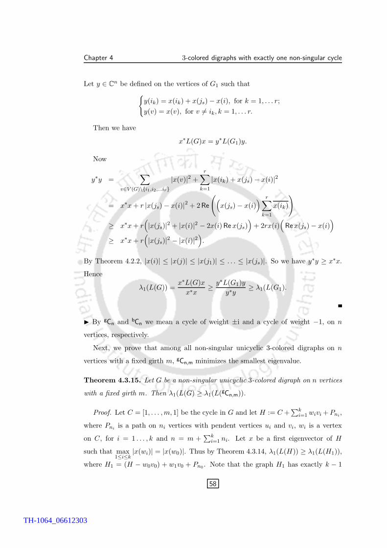
Chapter 4 3-colored digraphs with exactly one non-singular cycle
Let y ∈ Cn be defined on the vertices of G1 such that
{y(ik) = x(ik) + x(js) − x(i), for k = 1, . . . r;
y(v) = x(v), for v 6= ik, k = 1, . . . r.
Then we have
x∗L(G)x = y∗L(G1)y.
Now
y∗y =∑
v∈V (G)\{i1,i2,...ir}|x(v)|2 +
r∑
k=1
|x(ik) + x(js) − x(i)|2
= x∗x + r |x(js) − x(i)|2 + 2Re
((x(js) − x(i)
) r∑
k=1
x(ik)
)
≥ x∗x + r(|x(js)|2 + |x(i)|2 − 2x(i)Re x(js)
)+ 2rx(i)
(Rex(js) − x(i)
)
≥ x∗x + r(|x(js)|2 − |x(i)|2
).
By Theorem 4.2.2, |x(i)| ≤ |x(j)| ≤ |x(j1)| ≤ . . . ≤ |x(js)|. So we have y∗y ≥ x∗x.
Hence
λ1(L(G)) =x∗L(G)x
x∗x≥ y∗L(G1)y
y∗y≥ λ1(L(G1).
◮ By gCn and bCn we mean a cycle of weight ±i and a cycle of weight −1, on n
vertices, respectively.
Next, we prove that among all non-singular unicyclic 3-colored digraphs on n
vertices with a fixed girth m, gCn,m minimizes the smallest eigenvalue.
Theorem 4.3.15. Let G be a non-singular unicyclic 3-colored digraph on n vertices
with a fixed girth m. Then λ1(L(G) ≥ λ1(L(gCn,m)).
Proof. Let C = [1, . . . ,m, 1] be the cycle in G and let H := C +∑k
i=1 wivi + Pni,
where Pniis a path on ni vertices with pendent vertices ui and vi, wi is a vertex
on C, for i = 1 . . . , k and n = m +∑k
i=1 ni. Let x be a first eigenvector of H
such that max1≤i≤k
|x(wi)| = |x(w0)|. Thus by Theorem 4.3.14, λ1(L(H)) ≥ λ1(L(H1)),
where H1 = (H − w0v0) + w1v0 + Pn0. Note that the graph H1 has exactly k − 1
58
TH-1064_06612303
Chapter 4 3-colored digraphs with exactly one non-singular cycle
paths attached to k − 1 vertices of the cycle. By Lemma 4.1.16, λ1(L(bCn,m)) ≥λ1(L(gCn,m)). Thus with similar argument, after a finite number of steps we have
λ1(L(H)) ≥ λ1(L(H1)) ≥ · · · ≥ λ1(L(gCn,m)). Note that λ1(L(G)) ≥ λ1(L(H)), by
Lemma 4.3.14. Hence the result holds.
Definition 4.3.16. Consider the path Pn, n ≥ 3 on vertices 1, . . . , n. Add the blue
colored edge joining the vertices k and n − k + 1 of Pn, for 1 ≤ k < n2 to obtain a
mixed graph. We denote this graph by G(n, k).
Example 4.3.17. Mixed graphs G(7, 3) and G(8, 4) are supplied in the following
picture.
b
b
b
b
b
b
b
b
12
65
3
4
7
G(7, 3)
b
b b b b
b b b
1234
5 6 7 8
G(8, 2)
The following Lemma is essentially contained in [22, Theorem 3.4].
Lemma 4.3.18. Consider the b-lollipop graph bCn,m. Then the following holds:
(i) Multiplicity of the smallest Laplacian eigenvalue of bCn,m is one, for m < n.
(ii) If x is a first eigenvector of bCn,m, then x(i) = −x(m− i), for i = 1, . . . ,m− 1.
(iii) λ1(L(bCn,m−1)) < λ1(L(bCn,m)), for m > 3.
In the next lemma, we prove that λ1(L(G(n, k))) = a(Pn), for each k.
Lemma 4.3.19. Consider the mixed graph G(n, k) as in Definition 4.3.16
(i) λ1(L(G(n, k))) has multiplicity one, for each k 6= 1.
(ii) λ1(L(G(n, k)) = a(Pn),
Proof. (i) Let Y be a first eigenvector of G(n, k). If possible, suppose that
Y (n) = 0. Then by the eigen-conditions at the vertices n, n − 1, . . . , n − k + 2, it
59
TH-1064_06612303
Chapter 4 3-colored digraphs with exactly one non-singular cycle
follows that Y (n − k + 1) = Y (n − k + 2) = · · · = Y (n) = 0. So λ1(L(G(n, k))
is an eigenvalue of bCn−k+1,n−2k+2 with Y ′ = [Y (1), Y (2), · · · , Y (n − k + 1)]t
as an
eigenvector. Thus λ1(L(bCn−k+1,n−2k+2)) ≤ λ1(L(G(n, k))). By Lemma 4.3.1,
λ1(L(G(n, k))) ≤ λ1(L(bCn−k+1,n−2k+2)).
Hence λ1(L(G(n, k))) = λ1(L(bCn−k+1,n−2k+2)) and Y ′ is an eigenvector correspond-
ing to λ1(L(bCn−k+1,n−2k+2)). Observe that Y ′(k + 1) = −Y ′(n− k + 1), by Lemma
4.3.18(ii). Thus Y (k + 1) = −Y (n− k + 1) = 0, a contradiction to Lemma 4.2.9. So
Y (n) 6= 0 and hence λ1(L(G(n, k))) has multiplicity one, for k 6= 1, n.
(ii) Let y be a Fiedler vector of Pn. Then y(k) = −y(n − k + 1). Hence y
is an eigenvector of L(G(n, k)) corresponding to a(Pn). Thus λ1(L(G(n, k))) ≤a(Pn). If possible, suppose that λ1(L(G(n, k))) 6= a(Pn). Let z be an eigenvector
of L(G(n, k)) with ztz = 1 corresponding to λ1(L(G(n, k))). Then a(Pn)ytz =
ytL(G(n, k))z = λ1(L(G(n, k)))ytz and hence ytz = 0. Let 1√n11, y2, . . . , yn be the
normalized eigenvectors of L(Pn) corresponding to eigenvalues 0, λ2 = a(Pn), . . . , λn.
As ytz = 0 and z 6= α11, for α ∈ R, we see that z = α111√n
+α3y3 + . . .+αnyn, where
at least one αi 6= 0, for 2 < i ≤ n. Observe that
λ1(L(G(n, k))) = ztL(Pn)z + [z(k) + z(n − k + 1)]2
= [α23λ3 + . . . α2
nλn] + [z(k) + z(n − k + 1)]2
> a(Pn)[1 − α21] + α2
1
4
n= a(Pn) + α2
1
[4
n− a(Pn)
]
> a(Pn), as it can be seen that4
n> 2(1 − cos
π
n) = a(Pn),
a contradiction. Hence the result holds.
Lemma 4.3.20. λ1(L(gCn,m)) ≥ λ1(L(gCn)).
Proof. Let x ∈ Cn be a first eigenvector of gCn,m such that Imx(m) = 0. Thus
by Theorem 4.2.5, Rex(m) 6= 0 and Imx(m) = Im x(m + 1) = · · · = Imx(n) =
0. By Theorem 3.1.10, λ1(L(gCn,m)) = λ1(L(G[g])), and Y =
[Rex
− Imx
]is a first
eigenvector of G[g], where G=gCn,m. Note that Y (m′) = Y (m′ + 1) = · · · = Y (n′) =
0. Thus λ1(L(gCn,m)) = λ1(L(G[g])) = λ1(L(bCn+m,2m)). Using Lemma 4.3.1 and
60
TH-1064_06612303
Chapter 4 3-colored digraphs with exactly one non-singular cycle
Lemma 4.3.19(ii) we have, λ1(L(bCn+m,2m)) ≥ λ1(L(G(2n, n − m + 1))) = a(P2n).
Hence λ1(L(gCn,m)) = λ1(L(bCn+m,2m)) ≥ a(P2n) = 2(1 − cos π2n
). By Lemma 4.3.3,
λ1(L(gCn)) = 2(1 − cos π2n
). Hence λ1(L(gCn,m)) ≥ λ1(L(gCn)).
The next lemma follows from Theorem 4.3.15 and Lemma 4.3.20.
Lemma 4.3.21. Let G be a unicyclic 3-colored digraph on n vertices. Then
λ1(L(G)) ≥ 2(1 − cosπ
2n).
Equality holds if and only if G is a cycle gCn.
Next Theorem is our main result of this section which provides the unique graph
minimzing the smallest Laplacian eigenvalue over all non-singular unicyclic 3-colored
digraphs on n vertices.
Theorem 4.3.22. Among all non-singular unicyclic 3-colored digraphs on n ver-
tices, the smallest Laplacian eigenvalue is minimized by the cycle gCn.
Proof. Proof follows from Lemma 4.3.21.
4.4 Maximizing the smallest Laplacian eigenvalue over
unicyclic 3-colored digraphs
In this section we obtain the non-singular unicyclic 3-colored digraph maximizing
the smallest Laplacian eigenvalue over all non-singular unicyclic 3-colored digraph
on n vertices with a fixed girth.
Lemma 4.4.1. Let G be a non-singular unicyclic 3-colored digraph on n > 4 ver-
tices. Let T be a tree on k vertices which is not a star attached to a vertex v on the
cycle. Replace T with a star K1,k on k vertices in G in such a way that v is the
center of K1,k and call the resulting graph G′. Then λ1(L(G′)) > λ1(L(G)).
Proof. Let v = v1, v2, . . . , vk be the vertices of T such that vv2 ∈ E(T ). Let x
be a first eigenvector of G′. By Lemmas 4.3.9 and 4.3.10, λ1(L(G′)) < 1. Hence by
61
TH-1064_06612303
Chapter 4 3-colored digraphs with exactly one non-singular cycle
eigen-condition at the vertices vi, we have x(v2) = · · · = x(vk). Let dv and d′v be
the degrees of the vertex v in G and G′, respectively. Note that dv < d′v. Thus
λ1(L(G′)) = x∗L(G′)x
= x∗L(G′ − E(K1,k))x +
k∑
r=2
|x(v) − x(v2)|2
= x∗L(G′ − E(K1,k))x + (d′v − 2)|x(v) − x(v2)|2
> x∗L(G′ − E(K1,k))x + (dv − 2)|x(v) − x(v2)|2
= x∗L(G′ − E(K1,k))x +∑
vivj∈E(T )
|x(vi) − x(vj)|2 = x∗L(G)x
≥ λ1(L(G))
Applying Lemma 4.3.14 repeatedly and then using Lemma 4.1.16, we obtain the
following result which is a generalization of [18, Theorem 3.4].
Theorem 4.4.2. Among all non-singular unicyclic 3-colored digraphs with a fixed
girth m, the smallest Laplacian eigenvalue is maximized by a non-singular unicyclic
3-colored digraph of girth m with the following property: weight of the cycle is −1
and each vertex on the cycle is adjacent only to a non-negative number of pendent
vertices out side the cycle.
4.5 Unicyclic 3-colored digraph with second smallest
Laplacian eigenvalue equal to 1
In this section we obtain the non-singular unicyclic 3-colored digraphs G that have
second smallest Laplacian eigenvalue greater than 1, less than 1 and equal to 1.
Lemma 4.5.1. Let G be a non-singular unicyclic 3-colored digraph with a fixed girth
m. Let C be the non-singular cycle in G. Then the following holds.
(i) If m ≥ 4 and wC = −1, then λ2(L(G)) < 1.
(ii) If m ≥ 5 and wC = ±i, then λ2(L(G)) < 1.
62
TH-1064_06612303
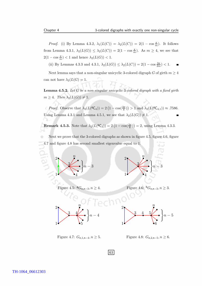
Chapter 4 3-colored digraphs with exactly one non-singular cycle
Proof. (i) By Lemma 4.3.2, λ1(L(C)) = λ2(L(C)) = 2(1 − cos πm
). It follows
from Lemma 4.3.1, λ2(L(G)) ≤ λ2(L(C)) = 2(1 − cos πm
). As m ≥ 4, we see that
2(1 − cos πm
) < 1 and hence λ2(L(G)) < 1.
(ii) By Lemmas 4.3.3 and 4.3.1, λ2(L(G)) ≤ λ2(L(C)) = 2(1 − cos 3π2m
) < 1.
Next lemma says that a non-singular unicyclic 3-colored digraph G of girth m ≥ 4
can not have λ2(L(G) = 1.
Lemma 4.5.2. Let G be a non-singular unicyclic 3-colored digraph with a fixed girth
m ≥ 4. Then λ2(L(G)) 6= 1.
Proof. Observe that λ2(L(gC4)) = 2(1 − cos(3π
8 ))
> 1 and λ2(L(gC4,1)) ≈ .7586.
Using Lemma 4.3.1 and Lemma 4.5.1, we see that λ2(L(G)) 6= 1.
Remark 4.5.3. Note that λ2(L(gC3)) = 2(1 − cos(3π
6 ))
= 2, using Lemma 4.3.3.
Next we prove that the 3-colored digraphs as shown in figure 4.5, figure 4.6, figure
4.7 and figure 4.8 has second smallest eigenvalue equal to 1.
b
b
b b
b
b
bb }
n − 3
2
1
3
4
n
Figure 4.5: gGn,n−3, n ≥ 4.
b
b
b b
b
b
bb }
n − 3
2
1
3
4
n
Figure 4.6: bGn,n−3, n ≥ 3.
b
b
b b b
bb
b
b
1
2
3 4
5
n}
n − 4
Figure 4.7: Gn,1,n−4, n ≥ 5.
b
b
b b b b
bb
b
b
1
2
3 4 5
n
6
}n − 5
Figure 4.8: Gn,2,n−5, n ≥ 6.
63
TH-1064_06612303
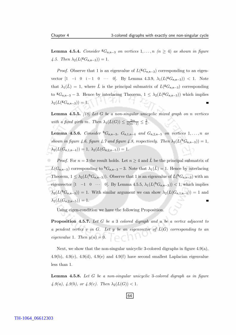
Chapter 4 3-colored digraphs with exactly one non-singular cycle
Lemma 4.5.4. Consider gGn,n−3 on vertices 1, . . . , n (n ≥ 4) as shown in figure
4.5. Then λ2(L(gGn,n−3)) = 1.
Proof. Observe that 1 is an eigenvalue of L(gGn,n−3) corresponding to an eigen-
vector [1 −i 0 i − 1 0 · · · 0]. By Lemma 4.3.9, λ1(L(gGn,n−3)) < 1. Note
that λ1(L) = 1, where L is the principal submatrix of L(gGn,n−3) corresponding
to gGn,n−3 − 3. Hence by interlacing Theorem, 1 ≤ λ2(L(gGn,n−3)) which implies
λ2(L(gGn,n−3)) = 1.
Lemma 4.5.5. [18] Let G be a non-singular unicyclic mixed graph on n vertices
with a fixed girth m. Then λ1(L(G)) ≤ 2mn(m−1) ≤ 3
n.
Lemma 4.5.6. Consider bGn,n−3, Gn,1,n−4 and Gn,2,n−5 on vertices 1, . . . , n as
shown in figure 4.6, figure 4.7 and figure 4.8, respectively. Then λ2(L(bGn,n−3)) = 1,
λ2(L(Gn,1,n−4)) = 1, λ2(L(Gn,2,n−5)) = 1.
Proof. For n = 3 the result holds. Let n ≥ 4 and L be the principal submatrix of
L(Gn,n−3) corresponding to bGn,n−3 − 3. Note that λ1(L) = 1. Hence by interlacing
Theorem, 1 ≤ λ2(L(bGn,n−3)). Observe that 1 is an eigenvalue of L(bGn,n−3) with an
eigenvector [1 −1 0 · · · 0]. By Lemma 4.5.5, λ1(L(bGn,n−3)) < 1, which implies
λ2(L(bGn,n−3)) = 1. With similar argument we can show λ2(L(Gn,1,n−4)) = 1 and
λ2(L(Gn,2,n−5)) = 1.
Using eigen-condition we have the following Proposition.
Proposition 4.5.7. Let G be a 3 colored digraph and u be a vertex adjacent to
a pendent vertex v in G. Let y be an eigenvector of L(G) corresponding to an
eigenvalue 1. Then y(u) = 0.
Next, we show that the non-singular unicyclic 3-colored digraphs in figure 4.9(a),
4.9(b), 4.9(c), 4.9(d), 4.9(e) and 4.9(f) have second smallest Laplacian eigenvalue
less than 1.
Lemma 4.5.8. Let G be a non-singular unicyclic 3-colored digraph as in figure
4.9(a), 4.9(b), or 4.9(c). Then λ2(L(G)) < 1.
64
TH-1064_06612303
Chapter 4 3-colored digraphs with exactly one non-singular cycle
b
b
b b
b
1
2
3 4
5
(a) b
b
b b
b
1
2
3 4
5
(b) b
b
b b b
1
2
3 4 5
(c)
b
b
b
b b b
1
2
3
4
5 6
(d)
b
b
b
b b b b
1
2
3
5
4 6 7
(e)
b
b
b
b b b b
1
2
3 74 5 6
(f)
Figure 4.9: Non-singular unicyclic 3-colored digraphs with λ2(L(G)) < 1.
Proof. Consider G as in figure 4.9(c). Note that λ2(L(G)) ≤ λ2(L(gG4,1)) = 1,
by Lemma 4.3.1 and Lemma 4.5.4. If possible, let 1 be an eigenvalue of L(G) with
an eigenvector y. Then y(4) = 0 by Proposition 4.5.7 and hence eigen-conditions
at the vertices we see that y(1) = y(2) = y(3) = −y(5) = 0, which is impossible.
Thus λ2(L(G)) < 1. Proofs for G as in figure 4.9(a) and 4.9(b) follows with similar
arguments.
Lemma 4.5.9. Let A =
[B CCt d
]be a symmetric matrix, where C is a vector
and d is real. Let there exist a vector U such that BU = 0 and CtU 6= 0. Then
In(A) = In(B)+(1, 1,−1), where In(A), In(B) denotes inertia of A,B, respectively.
Lemma 4.5.10. Let G be a non-singular unicyclic 3-colored digraph as shown in
figure 4.9(d) or figure 4.9(e). Then λ2(L(G)) < 1.
Proof. Consider G as in figure 4.9(d). Note that λ1(L) < 1, where L is the
principal submatrix of L(G) corresponding to G− 3. After a permutation similarity
operation we have,
L(G) =
[L CCt 4
]and L =
[L1 0 00 L2 00 0 1
], where Ct = [−1,−1,−1, 0,−1].
65
TH-1064_06612303
Chapter 4 3-colored digraphs with exactly one non-singular cycle
Observe that Ly = y and Cty 6= 0, where y = [0 0 0 0 1]. Thus by Lemma
4.5.9, L(G)− I has at least 2 negative eigenvalues, as L− I has at least one negative
eigenvalue. Hence λ2(L(G)) < 1. Similarly, if G is as in figure 4.9(e), we have
λ2(L(G)) < 1.
Lemma 4.5.11. Let G be a non-singular unicyclic 3-colored digraph as shown in
figure 4.9(f). Then λ2(L(G)) < 1.
Proof. Note that λ1(L) < 1, where L is the principal submatrix of L(G) corre-
sponding to G − 5. After a permutation similarity operation we have,
L(G) =
[L CCt 2
]and L =
[L1 00 L2
], where Ct = [0 0 0 −1 −1 0].
Observe that Ly = y and Cty 6= 0, where y = [1 0 1 1 0 0]. Thus by Lemma
4.5.9, L(G)− I has at least 2 negative eigenvalues, as L− I has at least one negative
eigenvalue. Hence λ2(L(G)) < 1.
We summarise our discussions to state the main result of this section.
Theorem 4.5.12. Let G be a non-singular unicyclic 3-colored digraph on n vertices.
Then λ2(L(G)) = 1 if and only if G is one of gGn,n−3,bGn,n−3, Gn,1,n−4 and Gn,2,n−5.
Proof. Assume that λ2(L(G)) = 1 and G is not any one of gGn,n−3,bGn,n−3,
Gn,1,n−4, Gn,2,n−5. By Lemma 4.5.2, girth of G is 3. Also, G 6= gC3, by Remark
4.5.3. Thus G can be obtained from one of the 3-colored digraphs as shown in figure
4.9(a), 4.9(b), 4.9(c), 4.9(d), 4.9(e) and 4.9(f) by adding pendents repeatedly. Thus
by Lemma 4.3.1 and Lemma 4.5.8, Lemma 4.5.10 or Lemma 4.5.11, λ2(G) < 1, a
contradiction. Converse follows from Lemma 4.5.4 and Lemma 4.5.6.
66
TH-1064_06612303
Chapter 5
Unicyclic 3-colored digraphs with SR-property
In Chapter 2 we have observed that the notion of 3-colored digraph is a general-
ization of the notion of mixed graph. The adjacency matrix of a 3-colored digraph
distinguishes the orientations of the green edges and hence spectral properties of
A(G) may supply some additional structural information about the graph. The
characteristic polynomial P (G;x) of an undirected graph has been studied by many
researchers (see for example [13]). The coefficients in P (G;x) have a combinatorial
interpretation in terms of the graph structure. In Section 5.1 we supply a combina-
torial interpretation of the coefficients of P (G;x) in terms of the graph structure,
for a 3-colored digraph G.
Definition 5.0.13. Let G be a 3-colored digraph and σ(G) be the multiset of
eigenvalues of A(G). We say G has SR-property if λ ∈ σ(G) if and only if 1λ∈ σ(G)
and both have the same multiplicity. It is understood that A(G) is non-singular.
In Section 5.2 we discuss the 3-colored digraphs satisfying SR-property. In Section
5.3 we supply the structure of the unicyclic 3-colored digraphs containing the cycle
of weight −1 satisfying SR-property. In Section 5.4 we supply the structure of the
unicyclic 3-colored digraphs containing the cycle of weight ±i satisfying SR-property.
5.1 Characteristic polynomial of A(G)
In this section we study the coefficients of the characteristic polynomial of a 3-colored
digraph. Recall that in defining subgraph, walk, path, matching, component, con-
nectedness, and degree of a vertex in G we focus only on the underlying unweighted
undirected graph of G.
67
TH-1064_06612303
Chapter 5 Unicyclic 3-colored digraphs with SR-property
Definition 5.1.1. We call a subgraph H linear if each component of H is either
an edge or a cycle. We call a component of a linear subgraph non-singular, if it is a
cycle of weight other than 1. All other components are called singular.1
◮ We use CH to mean the number of cycles in a linear subgraph H. By SH and
NH we mean the number of singular components and the number of non-singular
components in H, respectively.
◮ We use Ck to denote the set {H | H is a linear subgraph of order k of G in which
no cycle has weight ±i}.
Lemma 5.1.2. Let G be a 3-colored digraph. Then detA(G) =∑
H∈Cn
(−1)n−SH 2CH .
Proof. Note that det A(G) =∑
π sgn(π)a1,π(1) · · · an,π(n), where the summation
is taken over all permutations of {1, . . . , n}. Consider a permutation π giving a
nonzero contribution to det A(G). Note that each term in the cycle decomposition
of π, corresponds either to an edge or to a cycle of length at least 3 in G. As π(i) 6= i,
for any i, we see that π corresponds to a spanning linear subgraph of G.
Let H ′ be a linear subgraph of G containing a cycle C = [i1 · · · ik, i1] of weight
±i. Let π be a permutation corresponding to H ′. Take the permutation τ , sat-
isfying τ(i2) = i1, τ(i3) = i2, . . . , τ(ik) = ik−1, τ(i1) = ik, and τ(i) = π(i) for
i /∈ {i1, i2 . . . ik}. Then a1,π(1) · · · an,π(n) = −(a1,τ(1) . . . an,τ(n)
). Thus the contribu-
tion from linear subgraphs of G which contains at least one cycle of weight ±i, to
det A(G) is 0. Observe that a1,π(1) . . . an,π(n) = (−1)NH and sgn(π) = (−1)n−SH−NH ,
for each permutation π corresponding to a linear subgraph H of G without a cy-
cle of weight ±i. Since each linear subgraph H of G corresponds to exactly 2CH
permutations of {1 . . . , n}, we see that det A(G) =∑
H∈Cn(−1)n−SH 2CH .
◮ Henceforth, we understand that P (G;x) =∑n
i=0 aixn−i, a0 = 1.
Next, we describe the coefficients ai of P (G;x) generalizing Sachs theorem [13].
Theorem 5.1.3. Let G be a 3-colored digraph. Then ai =∑
H∈Ci
(−1)SH 2CH .
1They are actually Laplacian singular, see Theorem 2.1.11.
68
TH-1064_06612303
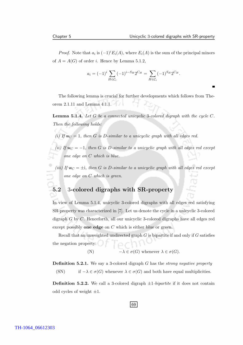
Chapter 5 Unicyclic 3-colored digraphs with SR-property
Proof. Note that ai is (−1)iEi(A), where Ei(A) is the sum of the principal minors
of A = A(G) of order i. Hence by Lemma 5.1.2,
ai = (−1)i∑
H∈Ci
(−1)i−SH 2CH =∑
H∈Ci
(−1)SH 2CH .
The following lemma is crucial for further developments which follows from The-
orem 2.1.11 and Lemma 4.1.1.
Lemma 5.1.4. Let G be a connected unicyclic 3-colored digraph with the cycle C.
Then the following holds:
(i) If wC = 1, then G is D-similar to a unicyclic graph with all edges red.
(ii) If wC = −1, then G is D-similar to a unicyclic graph with all edges red except
one edge on C which is blue.
(iii) If wC = ±i, then G is D-similar to a unicyclic graph with all edges red except
one edge on C which is green.
5.2 3-colored digraphs with SR-property
In view of Lemma 5.1.4, unicyclic 3-colored digraphs with all edges red satisfying
SR-property was characterized in [7]. Let us denote the cycle in a unicyclic 3-colored
digraph G by C. Henceforth, all our unicyclic 3-colored digraphs have all edges red
except possibly one edge on C which is either blue or green.
Recall that an unweighted undirected graph G is bipartite if and only if G satisfies
the negation property:
(N) −λ ∈ σ(G) whenever λ ∈ σ(G).
Definition 5.2.1. We say a 3-colored digraph G has the strong negative property
(SN) if −λ ∈ σ(G) whenever λ ∈ σ(G) and both have equal multiplicities.
Definition 5.2.2. We call a 3-colored digraph ±1-bipartite if it does not contain
odd cycles of weight ±1.
69
TH-1064_06612303
Chapter 5 Unicyclic 3-colored digraphs with SR-property
Lemma 5.2.3. Let G be a 3-colored digraph which is ±1-bipartite. Then G has
SN-property.
Proof. Consider P (G;x). By Theorem 5.1.3, a2i+1 = 0. Thus P (G;x) = xkq(x2),
for some integer k and polynomial q(x). Hence G has SN-property.
◮ Unlike the undirected case, converse of Lemma 5.2.3 is false. For example consider
G as shown in Figure 5.1. It has an odd cycle of weight ±1 and still has SN-property.
b
b
b b
b
b
G :
Figure 5.1: G has an odd cycle of weight ±1 and it has SN-property
However the situation is better for unicyclic graphs.
Lemma 5.2.4. Let G be a unicyclic 3-colored digraph. Then G has SN-property if
and only if G is ±1-bipartite.
Proof. Assume that G has SN-property. Hence a2ia2i+1 = 0, for each i. If possi-
ble, suppose that wC = ±1 and girth g = 2k+1. Then by Theorem 5.1.3, a2k+1 = ±2
and a2k = (−1)k|C2k|. Clearly C2k 6= ∅. Thus a2ka2k+1 6= 0, a contradiction. Hence
g is even. The converse follows from Lemma 5.2.3.
Definition 5.2.5. [26] Let H be a 3-colored digraph. For each j ∈ V (H) add a
new vertex j′ and add the edge (j, j′) of weight wj = ±1, i. We call the resulting
3-colored digraph a simple corona and denote it by H ◦ K1. A non-corona graph
means a graph that is not a simple corona.
Remark 5.2.6. Let H be a 3-colored and G = H ◦ K1. Put D = diag(w1, . . . , wn)
and D =
[I 0
0 D∗
]. Then A(G) =
[A(H) DD∗ 0
]and B = D∗A(G)D =
[A(H) I
I 0
].
Thus G is D-similar to the 3-colored digraph obtained from H by adding a pendent
vertex to each vertex i of H with an edge of color red. Henceforth, the newly
added edges in a simple corona are taken to be red. By [8, Lemma 2.1] − 1λ∈ σ(B)
whenever λ ∈ σ(B).
70
TH-1064_06612303
Chapter 5 Unicyclic 3-colored digraphs with SR-property
Lemma 5.2.7. Let H be a 3-colored, ±1-bipartite. Then H ◦ K1 has SR-property.
Proof. Follows using Lemma 5.2.3 and Remark 5.2.6.
It is natural to wonder whether a 3-colored digraph with SR-property is neces-
sarily a simple corona.
Lemma 5.2.8. Let G be a 3-colored digraph with SR-property. Then |ai| = |an−i|,for each i.
Proof. Similar to [7, Lemma 2.1].
◮ We denote the number of perfect matchings of a graph H by m0(H). For a graph
with a unique perfect matching we denote the perfect matching by M .
Definition 5.2.9. Let G be a 3-colored digraph with a unique perfect matching.
An alternating path P in G is a path of odd length such that alternate edges of
P (including the terminating edges) are in M . By PkG we denote the set of all
alternating paths of length at least k in G. By m1(G) we denote the number of
(n2 − 1)-matchings of G.
Definition 5.2.10. Let G be a connected unicyclic 3-colored digraph. For v ∈ V (G),
a component T of G − v which does not contain any other vertex of C is called a
tree branch at v. We say a tree branch is odd or even, if the order of the tree branch
is odd or even, respectively.
Lemma 5.2.11. Let G be a unicyclic 3-colored digraph satisfying SR-property. Then
m0(G) = 1. Furthermore, there is an odd tree branch of G at a vertex of the cycle
C.
Proof. If wC = 1, then in view of Lemma 5.1.4, this result is precisely Lemma
2.2 of [7]. If wC = −1, then the proof is similar to that of Lemma 2.2 of [7].
If wC = ±i, then by Theorem 5.1.2, ±1 = detA(G) = ±m0(G). Thus m0(G) = 1
and so n = 2m, for some integer m. Note that, if m0(G − C) > 0, then C must
be an even cycle, and hence m0(G) ≥ 2, not possible. Thus m0(G − C) = 0, which
implies the existence of a vertex u on C at which there is an odd tree branch.
71
TH-1064_06612303
Chapter 5 Unicyclic 3-colored digraphs with SR-property
Lemma 5.2.12. Let G be a connected 3-colored digraph on n = 2m vertices with
m0(G) = 1. Then m1(G) = m + |P3G| = |E(G)| + |P5
G|.
Proof. Put M = {e1, e2, . . . , em} and let f1, f2, . . . , fs be the remaining edges of
G. Note that any (m− 1)-subset of M contributes 1 to m1(G). Take an alternating
path in P3G, say, e1f1e2f2 . . . f2ke2k+1. Then {fj1, . . . , fjr−1
} ∪ M − {ei1 , . . . , eir} is
an (m − 1)-matching of G. Thus m1 ≥ n + |P3G|.
Conversely, take an (m − 1)-matching, say,
(∗) e1, . . . , ep, f1, . . . , fq.
Assume that eis have end vertices ui, vi. Put V = {up+1, . . . , um, vp+1, . . . , vm} and
E = {ep+1, . . . , em, f1, . . . , fq}. Consider H = (V,E). Note that |E| = |V | − 1.
Observation. No two eis in E have a common end vertex. Similarly, no two fjs
in E have a common end vertex.
Assume that H contains a cycle Γ. Then, in view of the previous observation, Γ
must be an even cycle containing eis and fjs alternately. This implies that G has
more than one perfect matchings. Not possible.
It follows that H is a tree. Then, in view of the previous observation, the maxi-
mum degree of a vertex in H is 2. Hence H is path. Obviously, it is an alternating
path.
Observe that H is nothing but the subgraph of G induced by the edges (and
their end vertices) in E. If there is another alternating path say H ′ which results in
the same (m− 1)-matching as in (∗), then E(H ′) must be {ep+1, . . . , em, f1, . . . , fq}.Hence H ′ is nothing but the subgraph induced by E. So H = H ′.
Hence m1(G) = m+|P3G|. The other equality follows as the number of alternating
paths of length 3 equals the number of non-matching edges.
◮ Let G be a unicyclic 3-colored digraph. By LG we mean the collection of all linear
subgraphs of G on n − 2 vertices containing C as one of its components.
Lemma 5.2.13. Let G be a 3-colored digraph with m0(G) = 1. The following
statements hold.
72
TH-1064_06612303
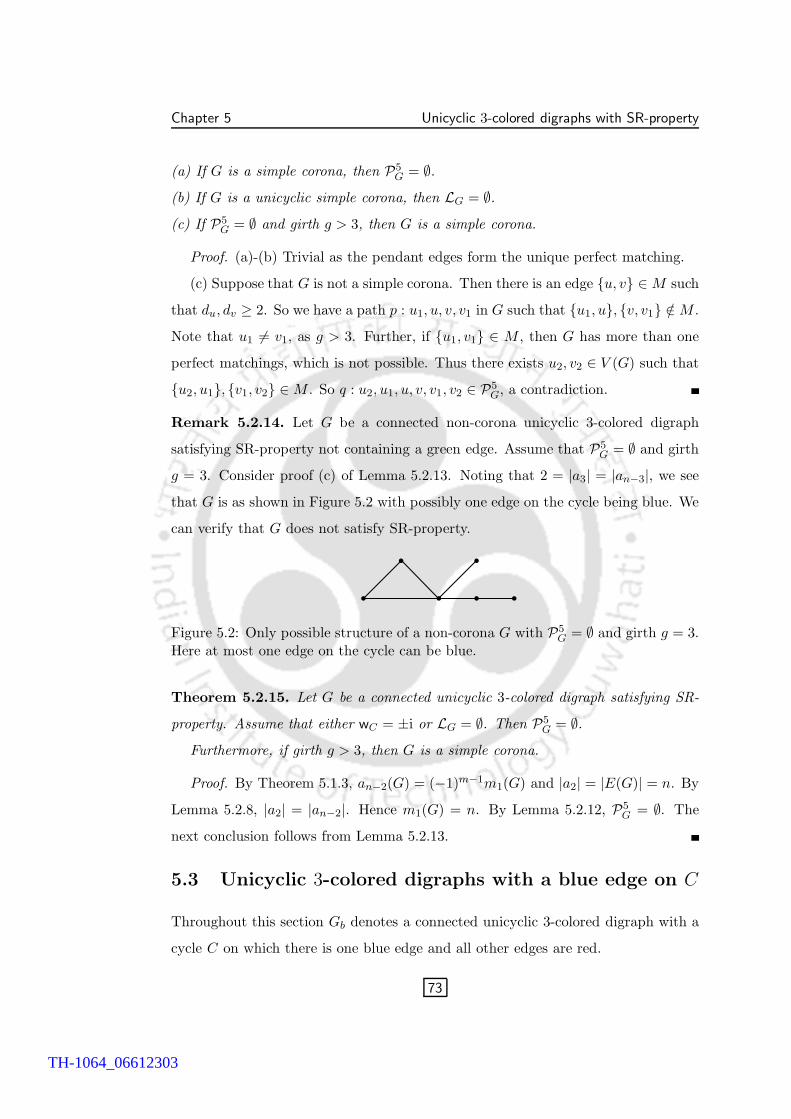
Chapter 5 Unicyclic 3-colored digraphs with SR-property
(a) If G is a simple corona, then P5G = ∅.
(b) If G is a unicyclic simple corona, then LG = ∅.(c) If P5
G = ∅ and girth g > 3, then G is a simple corona.
Proof. (a)-(b) Trivial as the pendant edges form the unique perfect matching.
(c) Suppose that G is not a simple corona. Then there is an edge {u, v} ∈ M such
that du, dv ≥ 2. So we have a path p : u1, u, v, v1 in G such that {u1, u}, {v, v1} /∈ M .
Note that u1 6= v1, as g > 3. Further, if {u1, v1} ∈ M , then G has more than one
perfect matchings, which is not possible. Thus there exists u2, v2 ∈ V (G) such that
{u2, u1}, {v1, v2} ∈ M . So q : u2, u1, u, v, v1, v2 ∈ P5G, a contradiction.
Remark 5.2.14. Let G be a connected non-corona unicyclic 3-colored digraph
satisfying SR-property not containing a green edge. Assume that P5G = ∅ and girth
g = 3. Consider proof (c) of Lemma 5.2.13. Noting that 2 = |a3| = |an−3|, we see
that G is as shown in Figure 5.2 with possibly one edge on the cycle being blue. We
can verify that G does not satisfy SR-property.
Figure 5.2: Only possible structure of a non-corona G with P5G = ∅ and girth g = 3.
Here at most one edge on the cycle can be blue.
Theorem 5.2.15. Let G be a connected unicyclic 3-colored digraph satisfying SR-
property. Assume that either wC = ±i or LG = ∅. Then P5G = ∅.
Furthermore, if girth g > 3, then G is a simple corona.
Proof. By Theorem 5.1.3, an−2(G) = (−1)m−1m1(G) and |a2| = |E(G)| = n. By
Lemma 5.2.8, |a2| = |an−2|. Hence m1(G) = n. By Lemma 5.2.12, P5G = ∅. The
next conclusion follows from Lemma 5.2.13.
5.3 Unicyclic 3-colored digraphs with a blue edge on C
Throughout this section Gb denotes a connected unicyclic 3-colored digraph with a
cycle C on which there is one blue edge and all other edges are red.
73
TH-1064_06612303
Chapter 5 Unicyclic 3-colored digraphs with SR-property
Lemma 5.3.1. Let G = Gb satisfy SR-property. The following statements hold.
(a) Girth g is even. Furthermore, if g ≡ 0 (mod 4), then G is a simple corona.
(b) |P5G| = 2|LG|.
(c) If G is not a simple corona, then G has exactly two odd tree branches at two
different vertices of the cycle.
Proof. (a) Similar to that of [7, Theorem 2.7].
(b) Similar to that of [7, Lemma 2.9].
(c) Similar to that of [7, Lemma 2.8].
Lemma 5.3.2. [7, Lemma 2.11] Let T be a tree such that T − v has a perfect
matching Mv and u be another vertex in T . Suppose that [v = v1, . . . , vr = u] is the
unique path from v to u in T . Then T − u has a perfect matching Mu if and only if
r = 2k + 1, for some k and the edges {v2i, v2i+1} ∈ Mv.
Lemma 5.3.3. Let T be a tree with |T | ≥ 3 odd, such that T − v has a perfect
matching M . Then there exist a pendent vertex u such that on the v-u-path [v =
v0, v1, . . . , v2k = u] in T , the edges {v2i+1, v2i+2} ∈ M , for i = 0, . . . , k − 1.
Proof. Take a vertex v1 adjacent to v in T . Then there exist a vertex v2 in T − v
such that {v1, v2} ∈ M , as T −v has perfect matching. If v2 is pendent then we take
u = v2. If not, take a vertex v3 adjacent to v2. Continuing similarly, after finitely
many steps we obtain u satisfying the statement.
Lemma 5.3.4. Let G = Gb satisfy SR-property. Assume that G is not a simple
corona. In view of Lemma 5.3.1, let Tu and Tv be the odd tree branches at vertices
u and v on C. Then |Tu| = |Tv| = 1 and the girth g = 6.
Proof. Let M be the unique perfect matching of G and let {u, u0}, {v, v0} ∈ M
where u0 ∈ Tu, v0 ∈ Tv. Note that each vertex w 6= u, v on C is matched to another
vertex of C and hence both the u0-v0-paths in G are alternating. Let p1, p2 be these
two paths. By Lemma 5.3.1, we see that g ≡ 2 (mod 4). Thus g ≥ 6 and hence
either case 1: one of p1, p2 has length at least 7 (say p1) or case 2: both have length
at least 5.
74
TH-1064_06612303
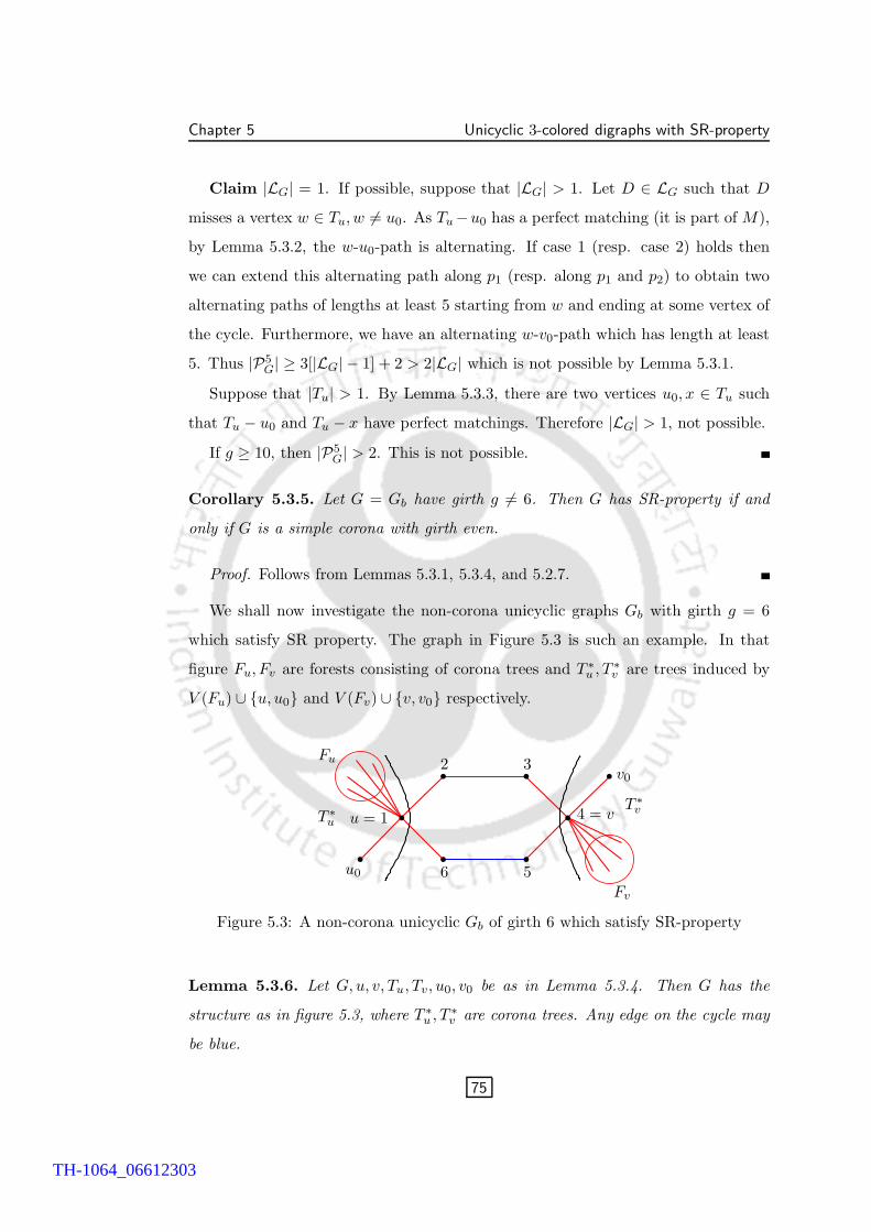
Chapter 5 Unicyclic 3-colored digraphs with SR-property
Claim |LG| = 1. If possible, suppose that |LG| > 1. Let D ∈ LG such that D
misses a vertex w ∈ Tu, w 6= u0. As Tu−u0 has a perfect matching (it is part of M),
by Lemma 5.3.2, the w-u0-path is alternating. If case 1 (resp. case 2) holds then
we can extend this alternating path along p1 (resp. along p1 and p2) to obtain two
alternating paths of lengths at least 5 starting from w and ending at some vertex of
the cycle. Furthermore, we have an alternating w-v0-path which has length at least
5. Thus |P5G| ≥ 3[|LG| − 1] + 2 > 2|LG| which is not possible by Lemma 5.3.1.
Suppose that |Tu| > 1. By Lemma 5.3.3, there are two vertices u0, x ∈ Tu such
that Tu − u0 and Tu − x have perfect matchings. Therefore |LG| > 1, not possible.
If g ≥ 10, then |P5G| > 2. This is not possible.
Corollary 5.3.5. Let G = Gb have girth g 6= 6. Then G has SR-property if and
only if G is a simple corona with girth even.
Proof. Follows from Lemmas 5.3.1, 5.3.4, and 5.2.7.
We shall now investigate the non-corona unicyclic graphs Gb with girth g = 6
which satisfy SR property. The graph in Figure 5.3 is such an example. In that
figure Fu, Fv are forests consisting of corona trees and T ∗u , T ∗
v are trees induced by
V (Fu) ∪ {u, u0} and V (Fv) ∪ {v, v0} respectively.
b
b
b
b
b
b
b
b
u0
v0
T ∗u
Fu
T ∗v
6 5Fv
2 3
u = 1 4 = v
Figure 5.3: A non-corona unicyclic Gb of girth 6 which satisfy SR-property
Lemma 5.3.6. Let G,u, v, Tu, Tv, u0, v0 be as in Lemma 5.3.4. Then G has the
structure as in figure 5.3, where T ∗u , T ∗
v are corona trees. Any edge on the cycle may
be blue.
75
TH-1064_06612303
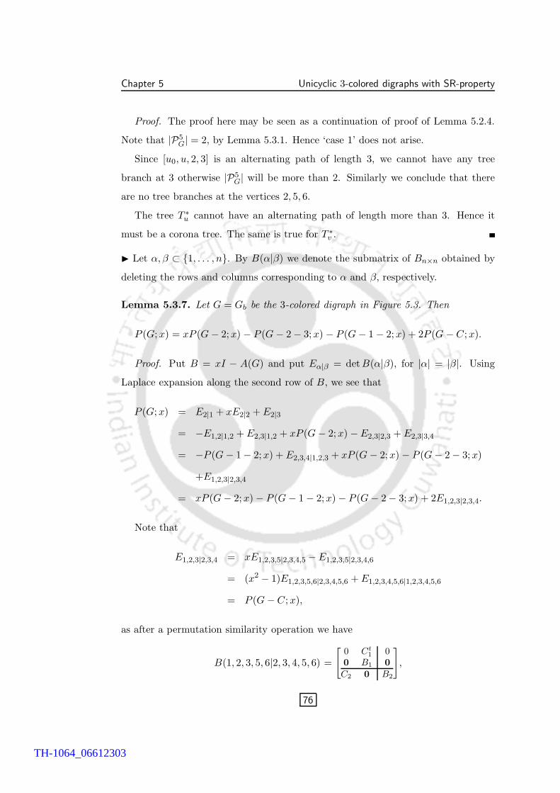
Chapter 5 Unicyclic 3-colored digraphs with SR-property
Proof. The proof here may be seen as a continuation of proof of Lemma 5.2.4.
Note that |P5G| = 2, by Lemma 5.3.1. Hence ‘case 1’ does not arise.
Since [u0, u, 2, 3] is an alternating path of length 3, we cannot have any tree
branch at 3 otherwise |P5G| will be more than 2. Similarly we conclude that there
are no tree branches at the vertices 2, 5, 6.
The tree T ∗u cannot have an alternating path of length more than 3. Hence it
must be a corona tree. The same is true for T ∗v .
◮ Let α, β ⊂ {1, . . . , n}. By B(α|β) we denote the submatrix of Bn×n obtained by
deleting the rows and columns corresponding to α and β, respectively.
Lemma 5.3.7. Let G = Gb be the 3-colored digraph in Figure 5.3. Then
P (G;x) = xP (G − 2;x) − P (G − 2 − 3;x) − P (G − 1 − 2;x) + 2P (G − C;x).
Proof. Put B = xI − A(G) and put Eα|β = detB(α|β), for |α| = |β|. Using
Laplace expansion along the second row of B, we see that
P (G;x) = E2|1 + xE2|2 + E2|3
= −E1,2|1,2 + E2,3|1,2 + xP (G − 2;x) − E2,3|2,3 + E2,3|3,4
= −P (G − 1 − 2;x) + E2,3,4|1,2,3 + xP (G − 2;x) − P (G − 2 − 3;x)
+E1,2,3|2,3,4
= xP (G − 2;x) − P (G − 1 − 2;x) − P (G − 2 − 3;x) + 2E1,2,3|2,3,4.
Note that
E1,2,3|2,3,4 = xE1,2,3,5|2,3,4,5 − E1,2,3,5|2,3,4,6
= (x2 − 1)E1,2,3,5,6|2,3,4,5,6 + E1,2,3,4,5,6|1,2,3,4,5,6
= P (G − C;x),
as after a permutation similarity operation we have
B(1, 2, 3, 5, 6|2, 3, 4, 5, 6) =
[0 Ct
1 00 B1 0
C2 0 B2
],
76
TH-1064_06612303
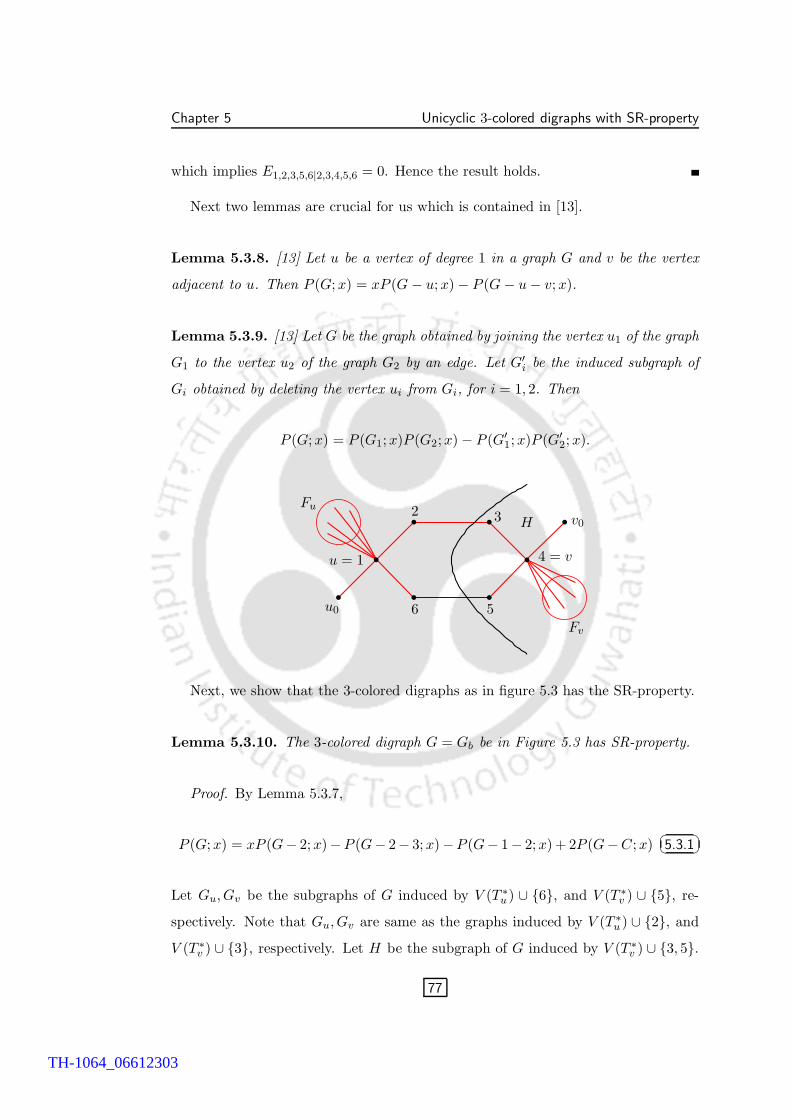
Chapter 5 Unicyclic 3-colored digraphs with SR-property
which implies E1,2,3,5,6|2,3,4,5,6 = 0. Hence the result holds.
Next two lemmas are crucial for us which is contained in [13].
Lemma 5.3.8. [13] Let u be a vertex of degree 1 in a graph G and v be the vertex
adjacent to u. Then P (G;x) = xP (G − u;x) − P (G − u − v;x).
Lemma 5.3.9. [13] Let G be the graph obtained by joining the vertex u1 of the graph
G1 to the vertex u2 of the graph G2 by an edge. Let G′i be the induced subgraph of
Gi obtained by deleting the vertex ui from Gi, for i = 1, 2. Then
P (G;x) = P (G1;x)P (G2;x) − P (G′1;x)P (G′
2;x).
b
b
b
b
b
b
b
b
u0
v0
Fu
Fv
6 5
2 3
u = 1 4 = v
H
Next, we show that the 3-colored digraphs as in figure 5.3 has the SR-property.
Lemma 5.3.10. The 3-colored digraph G = Gb be in Figure 5.3 has SR-property.
Proof. By Lemma 5.3.7,
P (G;x) = xP (G− 2;x)−P (G− 2− 3;x)−P (G− 1− 2;x) + 2P (G−C;x)�
�
�
�5.3.1
Let Gu, Gv be the subgraphs of G induced by V (T ∗u ) ∪ {6}, and V (T ∗
v ) ∪ {5}, re-
spectively. Note that Gu, Gv are same as the graphs induced by V (T ∗u ) ∪ {2}, and
V (T ∗v ) ∪ {3}, respectively. Let H be the subgraph of G induced by V (T ∗
v ) ∪ {3, 5}.
77
TH-1064_06612303
Chapter 5 Unicyclic 3-colored digraphs with SR-property
Using Lemma 5.3.8 and Lemma 5.3.9, we get
P (Gu;x) = xP (T ∗u ;x) − xP (Fu;x),
P (Gv;x) = xP (T ∗v ;x) − xP (Fv ;x),
P (H;x) = xP (Gv;x) − x2P (Fv;x) = x2P (T ∗v ;x) − 2x2P (Fv ;x),
P (G − 2;x) = P (Gu;x)P (H;x) − P (T ∗u ;x)P (Gv ;x),
P (G − 2 − 3;x) = P (Gu;x)P (Gv ;x) − P (T ∗u ;x)P (T ∗
v ;x),
P (G − 1 − 2;x) = xP (G − 1 − 2 − 6;x) − P (G − 1 − 2 − 6 − 5;x)
= x2P (Fu;x)P (H;x) − xP (Fu;x)P (Gv ;x),
and P (G − C;x) = x2P (Fu;x)P (Fv ;x)
Thus from equation 5.3.1, we see that
P (G;x) = (x2 − 1)2P (T ∗u ;x)P (T ∗
v ;x) + 4x4P (Fu;x)P (Fv ;x)
−2x2(x2 − 1) [P (T ∗u ;x)P (Fv ;x) + P (T ∗
v ;x)P (Fu;x)] .
By Lemma 5.2.7, T ∗u , T ∗
v and the trees in Fu, Fv have SR-property, as they are simple
corona trees. Let n=2m. Thus
P (T ∗u ;x)P (T ∗
v ;x) = (−1)m−2xn−4P
(T ∗
u ;1
x
)P
(T ∗
v ;1
x
),
P (T ∗u ;x)P (Fv ;x) = (−1)m−3xn−6P
(T ∗
u ;1
x
)P
(Fv;
1
x
),
P (T ∗v ;x)P (Fu;x) = (−1)m−3xn−6P
(T ∗
v ;1
x
)P
(Fu;
1
x
),
and P (Fu;x)P (Fv ;x) = (−1)m−4xn−8P
(Fu;
1
x
)P
(Fv;
1
x
).
This gives
(−1)mxnP
(G;
1
x
)= P (G;x).
Hence G has SR-property.
Theorem 5.3.11. Let G be a unicyclic 3-colored digraph with wC = −1. Then G
has SR-property if and only if either G is a simple corona of girth g = 2k, k ≥ 3 or
G has the structure as shown in figure 5.3, up to D-similarity.
Proof. Proof follows from Lemmas 5.3.1, 5.3.4, 5.2.7, 5.3.6 and 5.3.10.
78
TH-1064_06612303
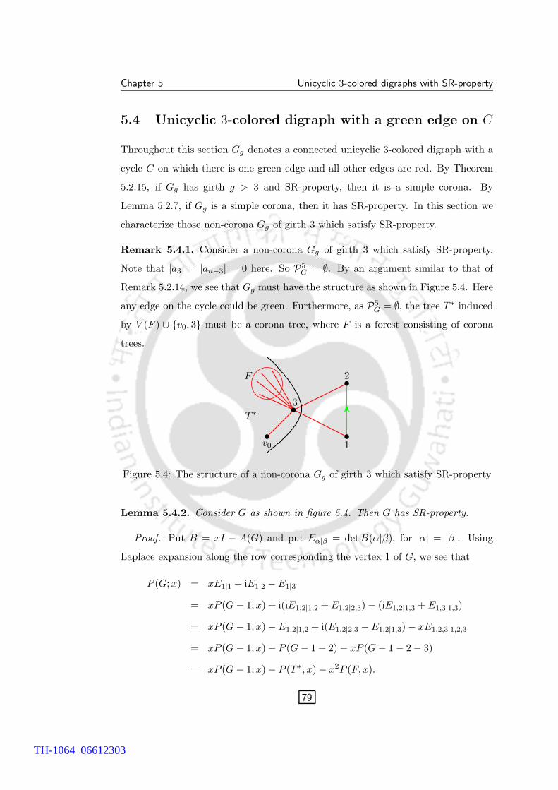
Chapter 5 Unicyclic 3-colored digraphs with SR-property
5.4 Unicyclic 3-colored digraph with a green edge on C
Throughout this section Gg denotes a connected unicyclic 3-colored digraph with a
cycle C on which there is one green edge and all other edges are red. By Theorem
5.2.15, if Gg has girth g > 3 and SR-property, then it is a simple corona. By
Lemma 5.2.7, if Gg is a simple corona, then it has SR-property. In this section we
characterize those non-corona Gg of girth 3 which satisfy SR-property.
Remark 5.4.1. Consider a non-corona Gg of girth 3 which satisfy SR-property.
Note that |a3| = |an−3| = 0 here. So P5G = ∅. By an argument similar to that of
Remark 5.2.14, we see that Gg must have the structure as shown in Figure 5.4. Here
any edge on the cycle could be green. Furthermore, as P5G = ∅, the tree T ∗ induced
by V (F ) ∪ {v0, 3} must be a corona tree, where F is a forest consisting of corona
trees.
b
b
b
b
3
2
1v0
F
T ∗
Figure 5.4: The structure of a non-corona Gg of girth 3 which satisfy SR-property
Lemma 5.4.2. Consider G as shown in figure 5.4. Then G has SR-property.
Proof. Put B = xI − A(G) and put Eα|β = detB(α|β), for |α| = |β|. Using
Laplace expansion along the row corresponding the vertex 1 of G, we see that
P (G;x) = xE1|1 + iE1|2 − E1|3
= xP (G − 1;x) + i(iE1,2|1,2 + E1,2|2,3) − (iE1,2|1,3 + E1,3|1,3)
= xP (G − 1;x) − E1,2|1,2 + i(E1,2|2,3 − E1,2|1,3) − xE1,2,3|1,2,3
= xP (G − 1;x) − P (G − 1 − 2) − xP (G − 1 − 2 − 3)
= xP (G − 1;x) − P (T ∗, x) − x2P (F, x).
79
TH-1064_06612303
Chapter 5 Unicyclic 3-colored digraphs with SR-property
Note that P (G − 1;x) = xP (T ∗;x) − xP (F ;x), using Lemma 5.3.8. Hence
P (G;x) = (x2 − 1)P (T ∗;x) − 2x2P (F ;x).
By Lemma 5.2.7, F and T ∗ have SR-property. Let n = 2m. Then
P (T ∗;x) = (−1)m−1xn−2P
(T ∗;
1
x
)
and P (F ;x) = (−1)m−2xn−4P
(F ;
1
x
)
Observe that (−1)mxnP(G; 1
x
)= P (G;x). Hence G has SR-property.
Theorem 5.4.3. Let G be a unicyclic 3-colored digraph with wC = ±i. Then G has
SR-property if and only if either G is a simple corona or G has the structure as in
figure 5.4 up to D-similarity.
Proof. Proof follows from Theorem 5.2.15, Remark 5.4.1, Lemma 5.2.7 and
Lemma 5.4.2
80
TH-1064_06612303
Bibliography
[1] N. Abreu, Old and new results on algebraic connectivity of graphs, Linear
Algebra and its Applications, 423 (2007), 53-73.
[2] W. N. Anderson and T. D. Morley, Eigenvalues of the Laplacian of a graph,
Linear and Multilinear Algebra, 18 (1985), 141-145.
[3] R. B. Bapat, Graphs and Matrices, Hindustan Book Agency, (2010).
[4] R. B. Bapat, J. W. Grossman and D. M. Kulkarni, Generalized Matrix Tree
Theorem for Mixed Graphs, Linear and Multilinear Algebra, 46 (1999), 299-312.
[5] R. B. Bapat, J. W. Grossman and D. M. Kulkarni, Edge Version of the Matrix
Tree Theorem for Trees, Linear and Multilinear Algebra, 47 (2000), 217-229.
[6] R. B. Bapat, S. Pati, Algebraic connectivity and characteristic set of a graph,
Linear and Multilinear Algebra, 45 (1998), 247-273.
[7] S. Barik, M. Nath, S. Pati, B.K. Sarma, Unicyclic graphs with the strong
reciprocal eigenvalue property, Electronic Journal of Linear Algebra, 17 (2008),
139-153.
[8] S. Barik, M. Neumann and S. Pati, On nonsingular trees and reciprocal eigen-
value property, Linear and Multilinear Algebra, 54 (2006), 453-465.
[9] S. Barik, S. Pati and B. K. Sarma, The spectrum of the corona of two graphs,
SIAM J. Discrete Math., 21 (2007), 47-56.
[10] A. Bernath, G. Joret, Well-balanced orientations of mixed graphs, Information
Processing Letters, 106 (2008), 149-151.
81
TH-1064_06612303
Bibliography
[11] N. Biggs, Algebraic Graph Theory, Second Edition, Cambridge University
Press, Cambridge, (1993).
[12] J. A. Bondy and U. S. R. Murty, Graph theory, Graduate Texts in Mathematics,
244, Springer, New York, (2008).
[13] D. M. Cvetkovic, M. Doob and H. Sachs, Spectra of Graphs, Academic Press,
NewYork, 1980.
[14] D. Cvetkovic, P. Rowlinson and S. K. Simic, Signless Laplacian of Finite
Graphs, Linear Algebra and its Applications, 423 (2007), 155-171.
[15] D. Cvetkovic ans S. Simic, Graph spectra in Computer Science, Linear Algebra
and its Applications, 434 (2011), 1545-1562.
[16] S. Fallat, S. Kirkland and S. Pati, Minimizing algebraic connectivity over con-
nected graphs with fixed girth, Discrete Mathematics, 254 (2002), 115-142.
[17] Y. Z. Fan, On eigenvectors of mixed graphs with exactly one nonsingular cycle,
Czechoslovak Mathematical Journal, 57 (2007), 1215-1222.
[18] Y. Z. Fan, On the least eigenvalue of a unicyclic mixed graph, Linear and
Multilinear Algebra, 53 (2005), 97-113.
[19] Y. Z. Fan, On spectral integral variations of mixed graphs, Linear Algebra and
its Applications, 374 (2003), 307-316.
[20] Y. Z. Fan, Largest eigenvalue of a unicyclic mixed graph, Appl. Math. J.
Chinese Univ. Ser. B, 19 (2004), 140-148.
[21] Y. Z. Fan, On spectral integral variations of graphs, Linear and Multilinear
Algebra, 50 (2002), 133-142.
[22] Y. Z. Fan, S. C. Gong, Y. Wang and Y. B. Gao, First eigenvalue and first
eigenvectors of a nonsingular unicyclic mixed graph, Discrete Mathematics,
309 (2009), 2479-2487.
82
TH-1064_06612303
Bibliography
[23] M. Fiedler, Algebraic connectivity of graphs, Czechoslovak Mathematical Jour-
nal, 23 (1973), 298-305.
[24] M. Fiedler, Eigenvectors of acyclic matrices, Czechoslovak Mathematical Jour-
nal, 25 (1975), 607-618.
[25] M. Fiedler, A property of eigenvectors of nonnegative symmetric matrices and
its application to graph theory, Czechoslovak Mathematical Journal, 25 (1975),
619-633.
[26] R. Frucht and F. Harary, On the corona of two graphs, Aequationes Mathe-
maticae, 4 (1970), 322-325.
[27] C. Godsil and G. Royle, Algebraic Graph Theory, Graduate Texts in Mathe-
matics, 207, Springer-Verlag, New York, (2001).
[28] R. Grone, R. Merris and V. S. Sunder, The Laplacian spectrum of a graph,
SIAM J. Matrix Anal. Appl., 11 (1990), 218-238.
[29] R. Grone and R. Merris, The Laplacian spectrum of a graph II*, SIAM J.
Discrete Math., 7 (1994), 221-229.
[30] J. M. Guo, W. C. Shiu and J. Li, Algebraic connectivity of lollipop graphs,
Linear Algebra and its Applications, 434 (2011), 2204-2210.
[31] F. Harary, Graph Theory, Addison- Wesley, (1969).
[32] R. A. Horn and C. R. Johnson, Matrix Analysis, Cambridge University Press,
(1985).
[33] S. Kirkland, Algebraic connectivity, in Handbook of Linear Algebra, L. Hogben,
ed. Chapman Hall/CRC, Boca Raton, (2007), 36-136-12.
[34] M. Marcus and H. Minc, A survey of Matrix theory and Matrix Inequalities,
Dover, New York, (1992).
83
TH-1064_06612303
Bibliography
[35] R. Merris, Laplacian matrices of graphs: a survey, Linear Algebra and its
Applications, 197-198 (1994), 143-176.
[36] R. Merris, A Survey of Graph Laplacians, Linear and Multilinear Algebra, 39
(1995), 19-31.
[37] R. Merris, Laplacian graph eigenvectors, Linear Algebra and its Applications,
278 (1998), 221-236.
[38] B. Mohar, Laplacian eigenvalues of graphs: a survey, Discrete Mathematics,
109 (1992), 171-183.
[39] B. Ries and D. de. Werra, On two coloring problems in mixed graphs, European
Journal of Combinatorics, 29 (2008), 712-725.
[40] Y. Y. Tan and Y. Z. Fan, On Edge Singularity and Eigenvectors of Mixed
Graphs, Acta Mathematica Sinica, English series, 24 (2008), 139-146.
[41] X. D. Zhang and J. S. Li, The Laplacian spectrum of a mixed graph, Linear
Algebra and its Applications, 353 (2002), 11-20.
[42] X. D. Zhang and R. Luo, The Laplacian eigenvalues of mixed graphs, Linear
Algebra and its Applications, 362 (2003), 109-119.
84
TH-1064_06612303