Embed Size (px)
Citation preview

Spectra of periodic quantum graphs:more than one would expect
Pavel Exner
Doppler Institutefor Mathematical Physics and Applied Mathematics
Prague
in collaboration with Daniel Vasata, Milos Tater, and Ondrej Turek
A talk at the conference Differential Operators on Graphs and Waveguides
Graz, February 25, 2019
P.E.: Spectra of periodic graphs DOGW 2019 Graz February 25, 2019 - 1 -

Motivation
It is a standard part of the quantum lore that spectrum of periodicsystem has a number of familiar properties:
it is absolutely continuousit has a band-and-gap structurein two- or more dimensional systems the number of open gapsis always finite by the Bethe-Sommerfled conjectureband edges are reached at the boundary of the Brillouin zoneor in its center
My message here is that if the system in question is a quantum graph,nothing of that needs to be true!
To demonstrate this, I am going to discuss simple examples, arrays andlattices. Should you feel this is not a deep enough mathematics, let mequote a – rather provocative – phrase of Michael Berry:
Only wimps specialize in the general case. Real scientists pursue examples.
P.E.: Spectra of periodic graphs DOGW 2019 Graz February 25, 2019 - 2 -

Motivation
It is a standard part of the quantum lore that spectrum of periodicsystem has a number of familiar properties:
it is absolutely continuous
it has a band-and-gap structurein two- or more dimensional systems the number of open gapsis always finite by the Bethe-Sommerfled conjectureband edges are reached at the boundary of the Brillouin zoneor in its center
My message here is that if the system in question is a quantum graph,nothing of that needs to be true!
To demonstrate this, I am going to discuss simple examples, arrays andlattices. Should you feel this is not a deep enough mathematics, let mequote a – rather provocative – phrase of Michael Berry:
Only wimps specialize in the general case. Real scientists pursue examples.
P.E.: Spectra of periodic graphs DOGW 2019 Graz February 25, 2019 - 2 -

Motivation
It is a standard part of the quantum lore that spectrum of periodicsystem has a number of familiar properties:
it is absolutely continuousit has a band-and-gap structure
in two- or more dimensional systems the number of open gapsis always finite by the Bethe-Sommerfled conjectureband edges are reached at the boundary of the Brillouin zoneor in its center
My message here is that if the system in question is a quantum graph,nothing of that needs to be true!
To demonstrate this, I am going to discuss simple examples, arrays andlattices. Should you feel this is not a deep enough mathematics, let mequote a – rather provocative – phrase of Michael Berry:
Only wimps specialize in the general case. Real scientists pursue examples.
P.E.: Spectra of periodic graphs DOGW 2019 Graz February 25, 2019 - 2 -

Motivation
It is a standard part of the quantum lore that spectrum of periodicsystem has a number of familiar properties:
it is absolutely continuousit has a band-and-gap structurein two- or more dimensional systems the number of open gapsis always finite by the Bethe-Sommerfled conjecture
band edges are reached at the boundary of the Brillouin zoneor in its center
My message here is that if the system in question is a quantum graph,nothing of that needs to be true!
To demonstrate this, I am going to discuss simple examples, arrays andlattices. Should you feel this is not a deep enough mathematics, let mequote a – rather provocative – phrase of Michael Berry:
Only wimps specialize in the general case. Real scientists pursue examples.
P.E.: Spectra of periodic graphs DOGW 2019 Graz February 25, 2019 - 2 -

Motivation
It is a standard part of the quantum lore that spectrum of periodicsystem has a number of familiar properties:
it is absolutely continuousit has a band-and-gap structurein two- or more dimensional systems the number of open gapsis always finite by the Bethe-Sommerfled conjectureband edges are reached at the boundary of the Brillouin zoneor in its center
My message here is that if the system in question is a quantum graph,nothing of that needs to be true!
To demonstrate this, I am going to discuss simple examples, arrays andlattices. Should you feel this is not a deep enough mathematics, let mequote a – rather provocative – phrase of Michael Berry:
Only wimps specialize in the general case. Real scientists pursue examples.
P.E.: Spectra of periodic graphs DOGW 2019 Graz February 25, 2019 - 2 -

Motivation
It is a standard part of the quantum lore that spectrum of periodicsystem has a number of familiar properties:
it is absolutely continuousit has a band-and-gap structurein two- or more dimensional systems the number of open gapsis always finite by the Bethe-Sommerfled conjectureband edges are reached at the boundary of the Brillouin zoneor in its center
My message here is that if the system in question is a quantum graph,nothing of that needs to be true!
To demonstrate this, I am going to discuss simple examples, arrays andlattices.
Should you feel this is not a deep enough mathematics, let mequote a – rather provocative – phrase of Michael Berry:
Only wimps specialize in the general case. Real scientists pursue examples.
P.E.: Spectra of periodic graphs DOGW 2019 Graz February 25, 2019 - 2 -

Motivation
It is a standard part of the quantum lore that spectrum of periodicsystem has a number of familiar properties:
it is absolutely continuousit has a band-and-gap structurein two- or more dimensional systems the number of open gapsis always finite by the Bethe-Sommerfled conjectureband edges are reached at the boundary of the Brillouin zoneor in its center
My message here is that if the system in question is a quantum graph,nothing of that needs to be true!
To demonstrate this, I am going to discuss simple examples, arrays andlattices. Should you feel this is not a deep enough mathematics, let mequote a – rather provocative – phrase of Michael Berry:
Only wimps specialize in the general case. Real scientists pursue examples.
P.E.: Spectra of periodic graphs DOGW 2019 Graz February 25, 2019 - 2 -

Motivation
It is a standard part of the quantum lore that spectrum of periodicsystem has a number of familiar properties:
it is absolutely continuousit has a band-and-gap structurein two- or more dimensional systems the number of open gapsis always finite by the Bethe-Sommerfled conjectureband edges are reached at the boundary of the Brillouin zoneor in its center
My message here is that if the system in question is a quantum graph,nothing of that needs to be true!
To demonstrate this, I am going to discuss simple examples, arrays andlattices. Should you feel this is not a deep enough mathematics, let mequote a – rather provocative – phrase of Michael Berry:
Only wimps specialize in the general case. Real scientists pursue examples.
P.E.: Spectra of periodic graphs DOGW 2019 Graz February 25, 2019 - 2 -

Something is obvious
The possible absolute continuity violation comes from the fact that theunique continuation principle may not hold in quantum graphs
, where onecan encounter the so-called Dirichlet eigenvalues
Courtesy: Peter Kuchment
The other claims are much less trivial and time will allow just to presentresults with brief hints about proof ideas
To show that the spectrum may be even pure point we consider our firstexample which concerns a chain graph in a magnetic field, in generalnonconstant
P.E.: Spectra of periodic graphs DOGW 2019 Graz February 25, 2019 - 3 -

Something is obvious
The possible absolute continuity violation comes from the fact that theunique continuation principle may not hold in quantum graphs, where onecan encounter the so-called Dirichlet eigenvalues
Courtesy: Peter Kuchment
The other claims are much less trivial and time will allow just to presentresults with brief hints about proof ideas
To show that the spectrum may be even pure point
we consider our firstexample which concerns a chain graph in a magnetic field, in generalnonconstant
P.E.: Spectra of periodic graphs DOGW 2019 Graz February 25, 2019 - 3 -

Something is obvious
The possible absolute continuity violation comes from the fact that theunique continuation principle may not hold in quantum graphs, where onecan encounter the so-called Dirichlet eigenvalues
Courtesy: Peter Kuchment
The other claims are much less trivial and time will allow just to presentresults with brief hints about proof ideas
To show that the spectrum may be even pure point we consider our firstexample which concerns a chain graph
in a magnetic field, in generalnonconstant
P.E.: Spectra of periodic graphs DOGW 2019 Graz February 25, 2019 - 3 -

Something is obvious
The possible absolute continuity violation comes from the fact that theunique continuation principle may not hold in quantum graphs, where onecan encounter the so-called Dirichlet eigenvalues
Courtesy: Peter Kuchment
The other claims are much less trivial and time will allow just to presentresults with brief hints about proof ideas
To show that the spectrum may be even pure point we consider our firstexample which concerns a chain graph in a magnetic field, in generalnonconstant
P.E.: Spectra of periodic graphs DOGW 2019 Graz February 25, 2019 - 3 -

The magnetic chainTo be specific, the chain graph will look as follows
0 π 0 π 0 π• • • •
eLj−1
eUj−1
Aj−1
eLj
eUj
Aj
eLj+1
eUj+1
Aj+1
vj−1 vj vj+1 vj+2
. . . . . .
The Hamiltonian is magnetic Laplacian, ψj 7→ −D2ψj on each graph link,where D := −i∇− A, and for definiteness we assume δ-coupling in thevertices, i.e. the domain consists of functions from H2
loc(Γ) satisfying
ψi (0) = ψj(0) =: ψ(0) , i , j ∈ n ,
n∑i=1
Dψi (0) = αψ(0) ,
where n = {1, 2, . . . , n} is the index set numbering the edges – in our casen = 4 – and α ∈ R is the coupling constant
This is a particular case of the general conditions that make the operatorself-adjoint [Kostrykin-Schrader’03]
P.E.: Spectra of periodic graphs DOGW 2019 Graz February 25, 2019 - 4 -

The magnetic chainTo be specific, the chain graph will look as follows
0 π 0 π 0 π• • • •
eLj−1
eUj−1
Aj−1
eLj
eUj
Aj
eLj+1
eUj+1
Aj+1
vj−1 vj vj+1 vj+2
. . . . . .
The Hamiltonian is magnetic Laplacian, ψj 7→ −D2ψj on each graph link,where D := −i∇− A
, and for definiteness we assume δ-coupling in thevertices, i.e. the domain consists of functions from H2
loc(Γ) satisfying
ψi (0) = ψj(0) =: ψ(0) , i , j ∈ n ,
n∑i=1
Dψi (0) = αψ(0) ,
where n = {1, 2, . . . , n} is the index set numbering the edges – in our casen = 4 – and α ∈ R is the coupling constant
This is a particular case of the general conditions that make the operatorself-adjoint [Kostrykin-Schrader’03]
P.E.: Spectra of periodic graphs DOGW 2019 Graz February 25, 2019 - 4 -

The magnetic chainTo be specific, the chain graph will look as follows
0 π 0 π 0 π• • • •
eLj−1
eUj−1
Aj−1
eLj
eUj
Aj
eLj+1
eUj+1
Aj+1
vj−1 vj vj+1 vj+2
. . . . . .
The Hamiltonian is magnetic Laplacian, ψj 7→ −D2ψj on each graph link,where D := −i∇− A, and for definiteness we assume δ-coupling in thevertices, i.e. the domain consists of functions from H2
loc(Γ) satisfying
ψi (0) = ψj(0) =: ψ(0) , i , j ∈ n ,
n∑i=1
Dψi (0) = αψ(0) ,
where n = {1, 2, . . . , n} is the index set numbering the edges – in our casen = 4 – and α ∈ R is the coupling constant
This is a particular case of the general conditions that make the operatorself-adjoint [Kostrykin-Schrader’03]
P.E.: Spectra of periodic graphs DOGW 2019 Graz February 25, 2019 - 4 -

The magnetic chainTo be specific, the chain graph will look as follows
0 π 0 π 0 π• • • •
eLj−1
eUj−1
Aj−1
eLj
eUj
Aj
eLj+1
eUj+1
Aj+1
vj−1 vj vj+1 vj+2
. . . . . .
The Hamiltonian is magnetic Laplacian, ψj 7→ −D2ψj on each graph link,where D := −i∇− A, and for definiteness we assume δ-coupling in thevertices, i.e. the domain consists of functions from H2
loc(Γ) satisfying
ψi (0) = ψj(0) =: ψ(0) , i , j ∈ n ,
n∑i=1
Dψi (0) = αψ(0) ,
where n = {1, 2, . . . , n} is the index set numbering the edges – in our casen = 4 – and α ∈ R is the coupling constant
This is a particular case of the general conditions that make the operatorself-adjoint [Kostrykin-Schrader’03]
P.E.: Spectra of periodic graphs DOGW 2019 Graz February 25, 2019 - 4 -

Floquet-Bloch analysis of the fully periodic case
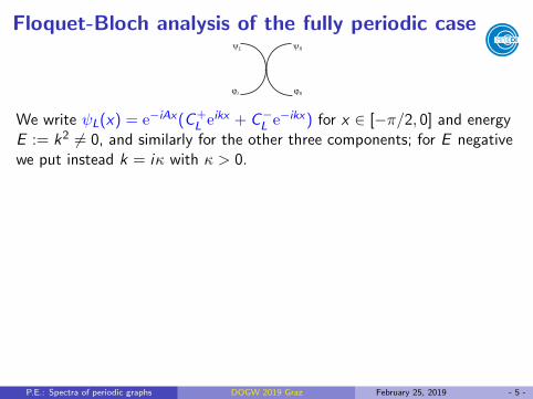
We write ψL(x) = e−iAx(C+L eikx + C−L e−ikx) for x ∈ [−π/2, 0] and energy
E := k2 6= 0, and similarly for the other three components
; for E negativewe put instead k = iκ with κ > 0.
The functions have to be matched through (a) the δ-coupling and (b)Floquet-Bloch conditions. This equation for the phase factor eiθ,
sin kπ cosAπ(e2iθ − 2ξ(k)eiθ + 1) = 0
with
ξ(k) :=1
cosAπ
(cos kπ +
α
4ksin kπ
),
for any k ∈ R ∪ iR \ {0} and the discriminant equal to D = 4(ξ(k)2 − 1)
Apart from the cases A− 12 ∈ Z and k ∈ N we have k2 ∈ σ(−∆α) iff the
condition |ξ(k)| ≤ 1 is satisfied.
P.E.: Spectra of periodic graphs DOGW 2019 Graz February 25, 2019 - 5 -
Floquet-Bloch analysis of the fully periodic case
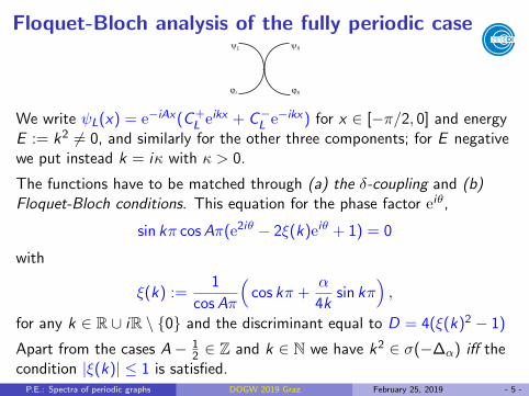
We write ψL(x) = e−iAx(C+L eikx + C−L e−ikx) for x ∈ [−π/2, 0] and energy
E := k2 6= 0, and similarly for the other three components; for E negativewe put instead k = iκ with κ > 0.
The functions have to be matched through (a) the δ-coupling and (b)Floquet-Bloch conditions. This equation for the phase factor eiθ,
sin kπ cosAπ(e2iθ − 2ξ(k)eiθ + 1) = 0
with
ξ(k) :=1
cosAπ
(cos kπ +
α
4ksin kπ
),
for any k ∈ R ∪ iR \ {0} and the discriminant equal to D = 4(ξ(k)2 − 1)
Apart from the cases A− 12 ∈ Z and k ∈ N we have k2 ∈ σ(−∆α) iff the
condition |ξ(k)| ≤ 1 is satisfied.
P.E.: Spectra of periodic graphs DOGW 2019 Graz February 25, 2019 - 5 -

Floquet-Bloch analysis of the fully periodic case
We write ψL(x) = e−iAx(C+L eikx + C−L e−ikx) for x ∈ [−π/2, 0] and energy
E := k2 6= 0, and similarly for the other three components; for E negativewe put instead k = iκ with κ > 0.
The functions have to be matched through (a) the δ-coupling and
(b)Floquet-Bloch conditions. This equation for the phase factor eiθ,
sin kπ cosAπ(e2iθ − 2ξ(k)eiθ + 1) = 0
with
ξ(k) :=1
cosAπ
(cos kπ +
α
4ksin kπ
),
for any k ∈ R ∪ iR \ {0} and the discriminant equal to D = 4(ξ(k)2 − 1)
Apart from the cases A− 12 ∈ Z and k ∈ N we have k2 ∈ σ(−∆α) iff the
condition |ξ(k)| ≤ 1 is satisfied.
P.E.: Spectra of periodic graphs DOGW 2019 Graz February 25, 2019 - 5 -

Floquet-Bloch analysis of the fully periodic case
We write ψL(x) = e−iAx(C+L eikx + C−L e−ikx) for x ∈ [−π/2, 0] and energy
E := k2 6= 0, and similarly for the other three components; for E negativewe put instead k = iκ with κ > 0.
The functions have to be matched through (a) the δ-coupling and (b)Floquet-Bloch conditions. This equation for the phase factor eiθ,
sin kπ cosAπ(e2iθ − 2ξ(k)eiθ + 1) = 0
with
ξ(k) :=1
cosAπ
(cos kπ +
α
4ksin kπ
),
for any k ∈ R ∪ iR \ {0} and the discriminant equal to D = 4(ξ(k)2 − 1)
Apart from the cases A− 12 ∈ Z and k ∈ N we have k2 ∈ σ(−∆α) iff the
condition |ξ(k)| ≤ 1 is satisfied.
P.E.: Spectra of periodic graphs DOGW 2019 Graz February 25, 2019 - 5 -
Floquet-Bloch analysis of the fully periodic case
We write ψL(x) = e−iAx(C+L eikx + C−L e−ikx) for x ∈ [−π/2, 0] and energy
E := k2 6= 0, and similarly for the other three components; for E negativewe put instead k = iκ with κ > 0.
The functions have to be matched through (a) the δ-coupling and (b)Floquet-Bloch conditions. This equation for the phase factor eiθ,
sin kπ cosAπ(e2iθ − 2ξ(k)eiθ + 1) = 0
with
ξ(k) :=1
cosAπ
(cos kπ +
α
4ksin kπ
),
for any k ∈ R ∪ iR \ {0} and the discriminant equal to D = 4(ξ(k)2 − 1)
Apart from the cases A− 12 ∈ Z and k ∈ N we have k2 ∈ σ(−∆α) iff the
condition |ξ(k)| ≤ 1 is satisfied.P.E.: Spectra of periodic graphs DOGW 2019 Graz February 25, 2019 - 5 -
In picture: determining the spectral bands
i 12 i
12
1 32
2 52
3 72
−4−2
2
4
ηγ > 0
γ = 0
γ ∈ (−8/π, 0)γ < −8/π
−→ √z ∈ R+0←− √z ∈ iR+
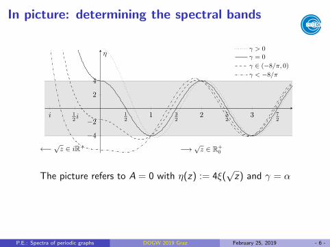
The picture refers to A = 0 with η(z) := 4ξ(√z) and γ = α
For A− 12 /∈ Z the situation is similar, just the width of the band changes
to 4 cosAπ, on the other hand, for A− 12 ∈ Z it shrinks to a line
P.E.: Spectra of periodic graphs DOGW 2019 Graz February 25, 2019 - 6 -
In picture: determining the spectral bands
i 12 i
12
1 32
2 52
3 72
−4−2
2
4
ηγ > 0
γ = 0
γ ∈ (−8/π, 0)γ < −8/π
−→ √z ∈ R+0←− √z ∈ iR+
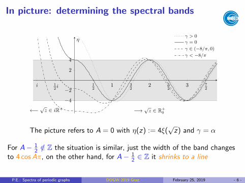
The picture refers to A = 0 with η(z) := 4ξ(√z) and γ = α
For A− 12 /∈ Z the situation is similar, just the width of the band changes
to 4 cosAπ, on the other hand, for A− 12 ∈ Z it shrinks to a line
P.E.: Spectra of periodic graphs DOGW 2019 Graz February 25, 2019 - 6 -

Duality
The idea was put forward by physicists – Alexander and de Gennes – andlater treated rigorously in [Cattaneo’97], [E’97], and [Pankrashkin’13]
We exclude possible Dirichlet eigenvalues from our considerationsassuming k ∈ K := {z : Im z ≥ 0 ∧ z /∈ Z}. On the one hand, we have thedifferential equation
(−∆α,A − k2)
(ψ(x , k)
ϕ(x , k)
)= 0
with the components referring to the upper and lower part of Γ, on theother hand the difference one
ψj+1(k) + ψj−1(k) = ξj(k)ψj(k) , k ∈ K ,
where ψj(k) := ψ(jπ, k) and ξ(k) was introduced above, ξj correspondingthe coupling αj . The two equations are intimately related.
P.E.: Spectra of periodic graphs DOGW 2019 Graz February 25, 2019 - 7 -

Duality
The idea was put forward by physicists – Alexander and de Gennes – andlater treated rigorously in [Cattaneo’97], [E’97], and [Pankrashkin’13]
We exclude possible Dirichlet eigenvalues from our considerationsassuming k ∈ K := {z : Im z ≥ 0 ∧ z /∈ Z}. On the one hand, we have thedifferential equation
(−∆α,A − k2)
(ψ(x , k)
ϕ(x , k)
)= 0
with the components referring to the upper and lower part of Γ,
on theother hand the difference one
ψj+1(k) + ψj−1(k) = ξj(k)ψj(k) , k ∈ K ,
where ψj(k) := ψ(jπ, k) and ξ(k) was introduced above, ξj correspondingthe coupling αj . The two equations are intimately related.
P.E.: Spectra of periodic graphs DOGW 2019 Graz February 25, 2019 - 7 -

Duality
The idea was put forward by physicists – Alexander and de Gennes – andlater treated rigorously in [Cattaneo’97], [E’97], and [Pankrashkin’13]
We exclude possible Dirichlet eigenvalues from our considerationsassuming k ∈ K := {z : Im z ≥ 0 ∧ z /∈ Z}. On the one hand, we have thedifferential equation
(−∆α,A − k2)
(ψ(x , k)
ϕ(x , k)
)= 0
with the components referring to the upper and lower part of Γ, on theother hand the difference one
ψj+1(k) + ψj−1(k) = ξj(k)ψj(k) , k ∈ K ,
where ψj(k) := ψ(jπ, k) and ξ(k) was introduced above, ξj correspondingthe coupling αj . The two equations are intimately related.
P.E.: Spectra of periodic graphs DOGW 2019 Graz February 25, 2019 - 7 -

Duality, continued
Theorem
Let αj ∈ R, then any solution
ψ(·, k)
ϕ(·, k)
with k2 ∈ R and k ∈ K satisfies
the difference equation, and conversely, the latter defines via(ψ(x , k)
ϕ(x , k)
)= e∓iA(x−jπ)
[ψj(k) cos k(x − jπ)
+(ψj+1(k)e±iAπ − ψj(k) cos kπ)sin k(x − jπ)
sin kπ
], x ∈
(jπ, (j + 1)π
),
solutions to the former satisfying the δ-coupling conditions. In addition,the former belongs to Lp(Γ) if and only if {ψj(k)}j∈Z ∈ `p(Z), the claimbeing true for both p ∈ {2,∞}.
On can generalize it to other chain graphs, for instance, with varyingmagnetic field, A = {Aj}j∈Z, the ring (half-)perimeters, ` = {`j}j∈Z, etc.
P.E.: Spectra of periodic graphs DOGW 2019 Graz February 25, 2019 - 8 -

Duality, continued
Theorem
Let αj ∈ R, then any solution
ψ(·, k)
ϕ(·, k)
with k2 ∈ R and k ∈ K satisfies
the difference equation, and conversely, the latter defines via(ψ(x , k)
ϕ(x , k)
)= e∓iA(x−jπ)
[ψj(k) cos k(x − jπ)
+(ψj+1(k)e±iAπ − ψj(k) cos kπ)sin k(x − jπ)
sin kπ
], x ∈
(jπ, (j + 1)π
),
solutions to the former satisfying the δ-coupling conditions. In addition,the former belongs to Lp(Γ) if and only if {ψj(k)}j∈Z ∈ `p(Z), the claimbeing true for both p ∈ {2,∞}.
On can generalize it to other chain graphs, for instance, with varyingmagnetic field, A = {Aj}j∈Z,
the ring (half-)perimeters, ` = {`j}j∈Z, etc.
P.E.: Spectra of periodic graphs DOGW 2019 Graz February 25, 2019 - 8 -

Duality, continued
Theorem
Let αj ∈ R, then any solution
ψ(·, k)
ϕ(·, k)
with k2 ∈ R and k ∈ K satisfies
the difference equation, and conversely, the latter defines via(ψ(x , k)
ϕ(x , k)
)= e∓iA(x−jπ)
[ψj(k) cos k(x − jπ)
+(ψj+1(k)e±iAπ − ψj(k) cos kπ)sin k(x − jπ)
sin kπ
], x ∈
(jπ, (j + 1)π
),
solutions to the former satisfying the δ-coupling conditions. In addition,the former belongs to Lp(Γ) if and only if {ψj(k)}j∈Z ∈ `p(Z), the claimbeing true for both p ∈ {2,∞}.
On can generalize it to other chain graphs, for instance, with varyingmagnetic field, A = {Aj}j∈Z, the ring (half-)perimeters, ` = {`j}j∈Z, etc.
P.E.: Spectra of periodic graphs DOGW 2019 Graz February 25, 2019 - 8 -

Example: a single flux alteredIt is believed that local perturbations give rise to eigenvalues in thegaps. While often true, it need not be the case generally.
We suppose that the field is modified on a single ring, i.e.A = {. . . ,A,A1,A . . . }, the we have a single simple eigenvalue in each gapprovided [E-Manko’17]
| cosA1π|| cosAπ| > 1 ,
otherwise the spectrum does not change.
In particular, the perturbation may give rise to no eigenvalues in gaps atall; note that this happens if the perturbed ring is ‘further from thenon-magnetic case’
Note also that the eigenvalue may split from the ac spectral band of theunperturbed system and lies between this band and the nearest eigenvalueof infinite multiplicity. When we change the magnetic field, the eigenvaluemay absorbed in the same band. On the other hand no eigenvalue emergesfrom the degenerate band.
P.E.: Spectra of periodic graphs DOGW 2019 Graz February 25, 2019 - 9 -
Example: a single flux alteredIt is believed that local perturbations give rise to eigenvalues in thegaps. While often true, it need not be the case generally.
We suppose that the field is modified on a single ring, i.e.A = {. . . ,A,A1,A . . . }, the we have a single simple eigenvalue in each gapprovided [E-Manko’17]
| cosA1π|| cosAπ| > 1 ,
otherwise the spectrum does not change.
In particular, the perturbation may give rise to no eigenvalues in gaps atall; note that this happens if the perturbed ring is ‘further from thenon-magnetic case’
Note also that the eigenvalue may split from the ac spectral band of theunperturbed system and lies between this band and the nearest eigenvalueof infinite multiplicity. When we change the magnetic field, the eigenvaluemay absorbed in the same band
. On the other hand no eigenvalue emergesfrom the degenerate band.
P.E.: Spectra of periodic graphs DOGW 2019 Graz February 25, 2019 - 9 -

Example: a single flux alteredIt is believed that local perturbations give rise to eigenvalues in thegaps. While often true, it need not be the case generally.
We suppose that the field is modified on a single ring, i.e.A = {. . . ,A,A1,A . . . }, the we have a single simple eigenvalue in each gapprovided [E-Manko’17]
| cosA1π|| cosAπ| > 1 ,
otherwise the spectrum does not change.
In particular, the perturbation may give rise to no eigenvalues in gaps atall; note that this happens if the perturbed ring is ‘further from thenon-magnetic case’
Note also that the eigenvalue may split from the ac spectral band of theunperturbed system and lies between this band and the nearest eigenvalueof infinite multiplicity. When we change the magnetic field, the eigenvaluemay absorbed in the same band. On the other hand no eigenvalue emergesfrom the degenerate band.
P.E.: Spectra of periodic graphs DOGW 2019 Graz February 25, 2019 - 9 -

Can periodic graphs have “wilder” spectra?Let us first recall the picture everybody knows
representing the spectrum of the difference operator associated with thealmost Mathieu equation
un+1 + un−1 + 2λ cos(2π(ω + nα))un = εun
for λ = 1, otherwise called Harper equation, as a function of α
P.E.: Spectra of periodic graphs DOGW 2019 Graz February 25, 2019 - 10 -

Can periodic graphs have “wilder” spectra?Let us first recall the picture everybody knows
representing the spectrum of the difference operator associated with thealmost Mathieu equation
un+1 + un−1 + 2λ cos(2π(ω + nα))un = εun
for λ = 1, otherwise called Harper equation, as a function of αP.E.: Spectra of periodic graphs DOGW 2019 Graz February 25, 2019 - 10 -

Nice mathematics, but do such things exist?Fractal nature of spectra for electron on a lattice in a homogeneousmagnetic field was conjectured by [Azbel’64] but it caught the imaginationonly after Hofstadter made the structure visible
It triggered a long and fruitful mathematical quest culminating by theproof of the Ten Martini Conjecture by Avila and Jitomirskaya in 2009,that is that the spectrum for an irrational field is a Cantor set
On the physical side, the effect remained theoretical for a long time andthought of in terms of the mentioned setting, with lattice and and ahomogeneous field providing the needed two length scales, genericallyincommensurable, from the lattice spacing and the cyclotron radius
The first experimental demonstration of such a spectral character wasdone instead in a microwave waveguide system with suitably placedobstacles simulating the almost Mathieu relation [Kuhl et al’98]
Only recently an experimental realization of the original concept wasachieved using a graphene lattice [Dean et al’13], [Ponomarenko’13]
P.E.: Spectra of periodic graphs DOGW 2019 Graz February 25, 2019 - 11 -

A chain with linear field growthSuppose that Aj = αj + θ holds for some α, θ ∈ R and every j ∈ Z
We need a stronger version of duality proved in [Pankrashkin’13] usingboundary triples: we exclude σD = {k2 : k ∈ N} and introduce
s(x ; z) =
{ sin(x√z)√
zfor z 6= 0,
x for z = 0,and c(x ; z) = cos(x
√z)
Theorem (after Pankrashkin’13)
For any interval J ⊂ R \ σD , the operator (Hγ,A)J is unitarily equivalentto the pre-image η(−1)
((LA)η(J)
), where LA is the operator on `2(Z)
acting as (LAqϕ)j = 2 cos(Ajπ)ϕj+1 + 2 cos(Aj−1π)ϕj−1 and
η(z) := γs(π; z) + 2c(π; z) + 2s ′(π; z)
Important: a simple gauge transformation shows that it is only thefractional part of Aj which matters. Consequently, the case of a rationalslope, α = p/q, is reduced to a periodic problem allowing the usualFloquet-Bloch treatment
P.E.: Spectra of periodic graphs DOGW 2019 Graz February 25, 2019 - 12 -

A chain with linear field growthSuppose that Aj = αj + θ holds for some α, θ ∈ R and every j ∈ ZWe need a stronger version of duality proved in [Pankrashkin’13] usingboundary triples: we exclude σD = {k2 : k ∈ N} and introduce
s(x ; z) =
{ sin(x√z)√
zfor z 6= 0,
x for z = 0,and c(x ; z) = cos(x
√z)
Theorem (after Pankrashkin’13)
For any interval J ⊂ R \ σD , the operator (Hγ,A)J is unitarily equivalentto the pre-image η(−1)
((LA)η(J)
), where LA is the operator on `2(Z)
acting as (LAqϕ)j = 2 cos(Ajπ)ϕj+1 + 2 cos(Aj−1π)ϕj−1 and
η(z) := γs(π; z) + 2c(π; z) + 2s ′(π; z)
Important: a simple gauge transformation shows that it is only thefractional part of Aj which matters. Consequently, the case of a rationalslope, α = p/q, is reduced to a periodic problem allowing the usualFloquet-Bloch treatment
P.E.: Spectra of periodic graphs DOGW 2019 Graz February 25, 2019 - 12 -
A chain with linear field growthSuppose that Aj = αj + θ holds for some α, θ ∈ R and every j ∈ ZWe need a stronger version of duality proved in [Pankrashkin’13] usingboundary triples: we exclude σD = {k2 : k ∈ N} and introduce
s(x ; z) =
{ sin(x√z)√
zfor z 6= 0,
x for z = 0,and c(x ; z) = cos(x
√z)
Theorem (after Pankrashkin’13)
For any interval J ⊂ R \ σD , the operator (Hγ,A)J is unitarily equivalentto the pre-image η(−1)
((LA)η(J)
), where LA is the operator on `2(Z)
acting as (LAqϕ)j = 2 cos(Ajπ)ϕj+1 + 2 cos(Aj−1π)ϕj−1 and
η(z) := γs(π; z) + 2c(π; z) + 2s ′(π; z)
Important: a simple gauge transformation shows that it is only thefractional part of Aj which matters
. Consequently, the case of a rationalslope, α = p/q, is reduced to a periodic problem allowing the usualFloquet-Bloch treatment
P.E.: Spectra of periodic graphs DOGW 2019 Graz February 25, 2019 - 12 -

A chain with linear field growthSuppose that Aj = αj + θ holds for some α, θ ∈ R and every j ∈ ZWe need a stronger version of duality proved in [Pankrashkin’13] usingboundary triples: we exclude σD = {k2 : k ∈ N} and introduce
s(x ; z) =
{ sin(x√z)√
zfor z 6= 0,
x for z = 0,and c(x ; z) = cos(x
√z)
Theorem (after Pankrashkin’13)
For any interval J ⊂ R \ σD , the operator (Hγ,A)J is unitarily equivalentto the pre-image η(−1)
((LA)η(J)
), where LA is the operator on `2(Z)
acting as (LAqϕ)j = 2 cos(Ajπ)ϕj+1 + 2 cos(Aj−1π)ϕj−1 and
η(z) := γs(π; z) + 2c(π; z) + 2s ′(π; z)
Important: a simple gauge transformation shows that it is only thefractional part of Aj which matters. Consequently, the case of a rationalslope, α = p/q, is reduced to a periodic problem allowing the usualFloquet-Bloch treatment
P.E.: Spectra of periodic graphs DOGW 2019 Graz February 25, 2019 - 12 -

The chain graph spectrumFor irrational slope duality allows to transform the problem into Harperequation. In this way we get in a cheap way a rather nontrivial result:
Theorem (E-Vasata’17)
Let Aj = αj + θ for some α, θ ∈ R and every j ∈ Z. Then for thespectrum σ(−∆γ,A) the following holds:
(a) If α, θ ∈ Z and γ = 0, then σac(−∆γ,A) = [0,∞) andσpp(−∆γ,A) = {n2| n ∈ N}(b) If γ 6= 0 and α = p/q with p, q relatively prime, αj + θ + 1
2 /∈ Z forall j = 0, . . . , q − 1, then −∆γ,A has infinitely degenerate ev’s {n2| n ∈ N}interlaced with an ac part consisting of q-tuples of closed intervals
(c) If the situation is as in (b) but αj + θ + 12 ∈ Z holds for some
j = 0, . . . , q − 1, then the spectrum σ(−∆γ,A) consists of infinitelydegenerate eigenvalues only, the Dirichlet ones plus q distinct others ineach interval (−∞, 1) and
(n2, (n + 1)2
).
P.E.: Spectra of periodic graphs DOGW 2019 Graz February 25, 2019 - 13 -

The chain graph spectrumFor irrational slope duality allows to transform the problem into Harperequation. In this way we get in a cheap way a rather nontrivial result:
Theorem (E-Vasata’17)
Let Aj = αj + θ for some α, θ ∈ R and every j ∈ Z. Then for thespectrum σ(−∆γ,A) the following holds:
(a) If α, θ ∈ Z and γ = 0, then σac(−∆γ,A) = [0,∞) andσpp(−∆γ,A) = {n2| n ∈ N}
(b) If γ 6= 0 and α = p/q with p, q relatively prime, αj + θ + 12 /∈ Z for
all j = 0, . . . , q − 1, then −∆γ,A has infinitely degenerate ev’s {n2| n ∈ N}interlaced with an ac part consisting of q-tuples of closed intervals
(c) If the situation is as in (b) but αj + θ + 12 ∈ Z holds for some
j = 0, . . . , q − 1, then the spectrum σ(−∆γ,A) consists of infinitelydegenerate eigenvalues only, the Dirichlet ones plus q distinct others ineach interval (−∞, 1) and
(n2, (n + 1)2
).
P.E.: Spectra of periodic graphs DOGW 2019 Graz February 25, 2019 - 13 -

The chain graph spectrumFor irrational slope duality allows to transform the problem into Harperequation. In this way we get in a cheap way a rather nontrivial result:
Theorem (E-Vasata’17)
Let Aj = αj + θ for some α, θ ∈ R and every j ∈ Z. Then for thespectrum σ(−∆γ,A) the following holds:
(a) If α, θ ∈ Z and γ = 0, then σac(−∆γ,A) = [0,∞) andσpp(−∆γ,A) = {n2| n ∈ N}(b) If γ 6= 0 and α = p/q with p, q relatively prime, αj + θ + 1
2 /∈ Z forall j = 0, . . . , q − 1, then −∆γ,A has infinitely degenerate ev’s {n2| n ∈ N}interlaced with an ac part consisting of q-tuples of closed intervals
(c) If the situation is as in (b) but αj + θ + 12 ∈ Z holds for some
j = 0, . . . , q − 1, then the spectrum σ(−∆γ,A) consists of infinitelydegenerate eigenvalues only, the Dirichlet ones plus q distinct others ineach interval (−∞, 1) and
(n2, (n + 1)2
).
P.E.: Spectra of periodic graphs DOGW 2019 Graz February 25, 2019 - 13 -

The chain graph spectrumFor irrational slope duality allows to transform the problem into Harperequation. In this way we get in a cheap way a rather nontrivial result:
Theorem (E-Vasata’17)
Let Aj = αj + θ for some α, θ ∈ R and every j ∈ Z. Then for thespectrum σ(−∆γ,A) the following holds:
(a) If α, θ ∈ Z and γ = 0, then σac(−∆γ,A) = [0,∞) andσpp(−∆γ,A) = {n2| n ∈ N}(b) If γ 6= 0 and α = p/q with p, q relatively prime, αj + θ + 1
2 /∈ Z forall j = 0, . . . , q − 1, then −∆γ,A has infinitely degenerate ev’s {n2| n ∈ N}interlaced with an ac part consisting of q-tuples of closed intervals
(c) If the situation is as in (b) but αj + θ + 12 ∈ Z holds for some
j = 0, . . . , q − 1, then the spectrum σ(−∆γ,A) consists of infinitelydegenerate eigenvalues only, the Dirichlet ones plus q distinct others ineach interval (−∞, 1) and
(n2, (n + 1)2
).
P.E.: Spectra of periodic graphs DOGW 2019 Graz February 25, 2019 - 13 -

The chain graph spectrum, continued
Theorem (E-Vasata’17, cont’d)
(d) If γ 6= 0 and α /∈ Q, then σ(−∆γ,A) does not depend on θ and it isa disjoint union of the isolated-point family {n2| n ∈ N} and Cantor sets,one inside each interval (−∞, 1) and
(n2, (n + 1)2
), n ∈ N. Moreover,
the overall Lebesgue measure of σ(−∆γ,A) is zero.
Furthermore, using a result of [Last-Shamis’16] one can also show
Proposition
Let Aj = αj + θ for some α, θ ∈ R and every j ∈ Z. There exist a denseGδ set of the slopes α for which, and all θ, the Haussdorff dimension
dimH σ(−∆γ,A) = 0
P.E.: Spectra of periodic graphs DOGW 2019 Graz February 25, 2019 - 14 -

Changing topic: graphs with a few gaps only
The graphs in the previous example had ‘many’ gaps indeed. Let usnow ask whether periodic graphs can have ‘just a few’ gaps
For ‘ordinary’ Schrodinger operators the dimension is decisive: the systemswhich are Z-periodic have generically an infinite number of open gaps,while Zν-periodic systems with ν ≥ 2 have only finitely many open gaps
This is the celebrated Bethe–Sommerfeld conjecture to which we havenowadays an affirmative answer in a large number of cases
In quantum graphs, ‘this is not a strict law’ by [Berkolaiko-Kuchment’13].For instance, we know that infinitely many gaps can by created by a graph‘decoration’, cf. [Schenker-Aizenman’00], [Kuchment’04]
The question arises, whether it is a ‘law’ at all?. In other words, do infiniteperiodic graphs having a finite nonzero number of open gaps exist? Fromobvious reasons we would call them Bethe–Sommerfeld graphs
P.E.: Spectra of periodic graphs DOGW 2019 Graz February 25, 2019 - 15 -

Changing topic: graphs with a few gaps only
The graphs in the previous example had ‘many’ gaps indeed. Let usnow ask whether periodic graphs can have ‘just a few’ gaps
For ‘ordinary’ Schrodinger operators the dimension is decisive
: the systemswhich are Z-periodic have generically an infinite number of open gaps,while Zν-periodic systems with ν ≥ 2 have only finitely many open gaps
This is the celebrated Bethe–Sommerfeld conjecture to which we havenowadays an affirmative answer in a large number of cases
In quantum graphs, ‘this is not a strict law’ by [Berkolaiko-Kuchment’13].For instance, we know that infinitely many gaps can by created by a graph‘decoration’, cf. [Schenker-Aizenman’00], [Kuchment’04]
The question arises, whether it is a ‘law’ at all?. In other words, do infiniteperiodic graphs having a finite nonzero number of open gaps exist? Fromobvious reasons we would call them Bethe–Sommerfeld graphs
P.E.: Spectra of periodic graphs DOGW 2019 Graz February 25, 2019 - 15 -

Changing topic: graphs with a few gaps only
The graphs in the previous example had ‘many’ gaps indeed. Let usnow ask whether periodic graphs can have ‘just a few’ gaps
For ‘ordinary’ Schrodinger operators the dimension is decisive: the systemswhich are Z-periodic have generically an infinite number of open gaps,
while Zν-periodic systems with ν ≥ 2 have only finitely many open gaps
This is the celebrated Bethe–Sommerfeld conjecture to which we havenowadays an affirmative answer in a large number of cases
In quantum graphs, ‘this is not a strict law’ by [Berkolaiko-Kuchment’13].For instance, we know that infinitely many gaps can by created by a graph‘decoration’, cf. [Schenker-Aizenman’00], [Kuchment’04]
The question arises, whether it is a ‘law’ at all?. In other words, do infiniteperiodic graphs having a finite nonzero number of open gaps exist? Fromobvious reasons we would call them Bethe–Sommerfeld graphs
P.E.: Spectra of periodic graphs DOGW 2019 Graz February 25, 2019 - 15 -
Changing topic: graphs with a few gaps only
The graphs in the previous example had ‘many’ gaps indeed. Let usnow ask whether periodic graphs can have ‘just a few’ gaps
For ‘ordinary’ Schrodinger operators the dimension is decisive: the systemswhich are Z-periodic have generically an infinite number of open gaps,while Zν-periodic systems with ν ≥ 2 have only finitely many open gaps
This is the celebrated Bethe–Sommerfeld conjecture to which we havenowadays an affirmative answer in a large number of cases
In quantum graphs, ‘this is not a strict law’ by [Berkolaiko-Kuchment’13].For instance, we know that infinitely many gaps can by created by a graph‘decoration’, cf. [Schenker-Aizenman’00], [Kuchment’04]
The question arises, whether it is a ‘law’ at all?. In other words, do infiniteperiodic graphs having a finite nonzero number of open gaps exist? Fromobvious reasons we would call them Bethe–Sommerfeld graphs
P.E.: Spectra of periodic graphs DOGW 2019 Graz February 25, 2019 - 15 -

Changing topic: graphs with a few gaps only
The graphs in the previous example had ‘many’ gaps indeed. Let usnow ask whether periodic graphs can have ‘just a few’ gaps
For ‘ordinary’ Schrodinger operators the dimension is decisive: the systemswhich are Z-periodic have generically an infinite number of open gaps,while Zν-periodic systems with ν ≥ 2 have only finitely many open gaps
This is the celebrated Bethe–Sommerfeld conjecture to which we havenowadays an affirmative answer in a large number of cases
In quantum graphs, ‘this is not a strict law’ by [Berkolaiko-Kuchment’13].For instance, we know that infinitely many gaps can by created by a graph‘decoration’, cf. [Schenker-Aizenman’00], [Kuchment’04]
The question arises, whether it is a ‘law’ at all?. In other words, do infiniteperiodic graphs having a finite nonzero number of open gaps exist?
Fromobvious reasons we would call them Bethe–Sommerfeld graphs
P.E.: Spectra of periodic graphs DOGW 2019 Graz February 25, 2019 - 15 -

Changing topic: graphs with a few gaps only
The graphs in the previous example had ‘many’ gaps indeed. Let usnow ask whether periodic graphs can have ‘just a few’ gaps
For ‘ordinary’ Schrodinger operators the dimension is decisive: the systemswhich are Z-periodic have generically an infinite number of open gaps,while Zν-periodic systems with ν ≥ 2 have only finitely many open gaps
This is the celebrated Bethe–Sommerfeld conjecture to which we havenowadays an affirmative answer in a large number of cases
In quantum graphs, ‘this is not a strict law’ by [Berkolaiko-Kuchment’13].For instance, we know that infinitely many gaps can by created by a graph‘decoration’, cf. [Schenker-Aizenman’00], [Kuchment’04]
The question arises, whether it is a ‘law’ at all?. In other words, do infiniteperiodic graphs having a finite nonzero number of open gaps exist? Fromobvious reasons we would call them Bethe–Sommerfeld graphs
P.E.: Spectra of periodic graphs DOGW 2019 Graz February 25, 2019 - 15 -
Scale-invariant coupling
The answer depends on the vertex coupling. Recall that the standardconditions for self-adjoint coupling of n edges at a vertex,
(U − I )Ψ + i(U + I )Ψ′ = 0 ,
where U is an n × n unitary matrix
. They decomposes into Dirichlet,Neumann, and Robin parts corresponding to eigenspaces of U witheigenvalues −1, 1, and the rest, respectively; if the latter is absent wecall such a coupling scale-invariant
Theorem ([E-Turek’17])
An infinite periodic quantum graph does not belong to the Bethe-Sommerfeld class if the couplings at its vertices are scale-invariant.
P.E.: Spectra of periodic graphs DOGW 2019 Graz February 25, 2019 - 16 -
Scale-invariant coupling
The answer depends on the vertex coupling. Recall that the standardconditions for self-adjoint coupling of n edges at a vertex,
(U − I )Ψ + i(U + I )Ψ′ = 0 ,
where U is an n × n unitary matrix. They decomposes into Dirichlet,Neumann, and Robin parts corresponding to eigenspaces of U witheigenvalues −1, 1, and the rest, respectively; if the latter is absent wecall such a coupling scale-invariant
Theorem ([E-Turek’17])
An infinite periodic quantum graph does not belong to the Bethe-Sommerfeld class if the couplings at its vertices are scale-invariant.
P.E.: Spectra of periodic graphs DOGW 2019 Graz February 25, 2019 - 16 -

Proof idea
The spectrum is determined by secular equation [BB’15]: we define
F (k ; ~ϑ) := det(
I− ei(A+kL)S(k)),
where the 2E × 2E matrices A, L, and S are as follows: the diagonalmatrix L is given by the lengths of the directed edges (bonds) of Γ,
thediagonal A has entries e±iϑl at points of the ‘Brillouin torus identification’,all the others are zero, and finally, S is the bond scattering matrix
Then k2 ∈ σ(H) holds if there is a quasimomentum values ~ϑ ∈ (−π, π]ν)such that the equation F (k; ~ϑ) = 0 is satisfied
We note that F (k ; ~ϑ depends on ~ϑ and (k`0, k`1, . . . , k`d), where{`0, `1, . . . , `d}, d + 1 ≤ E are the mutually different edge lengths of Γ.If the `’s are rationally related, the function is periodic in k , hence ifthere is a gap, there are infinitely many of them
P.E.: Spectra of periodic graphs DOGW 2019 Graz February 25, 2019 - 17 -

Proof idea
The spectrum is determined by secular equation [BB’15]: we define
F (k ; ~ϑ) := det(
I− ei(A+kL)S(k)),
where the 2E × 2E matrices A, L, and S are as follows: the diagonalmatrix L is given by the lengths of the directed edges (bonds) of Γ, thediagonal A has entries e±iϑl at points of the ‘Brillouin torus identification’,all the others are zero
, and finally, S is the bond scattering matrix
Then k2 ∈ σ(H) holds if there is a quasimomentum values ~ϑ ∈ (−π, π]ν)such that the equation F (k; ~ϑ) = 0 is satisfied
We note that F (k ; ~ϑ depends on ~ϑ and (k`0, k`1, . . . , k`d), where{`0, `1, . . . , `d}, d + 1 ≤ E are the mutually different edge lengths of Γ.If the `’s are rationally related, the function is periodic in k , hence ifthere is a gap, there are infinitely many of them
P.E.: Spectra of periodic graphs DOGW 2019 Graz February 25, 2019 - 17 -

Proof idea
The spectrum is determined by secular equation [BB’15]: we define
F (k ; ~ϑ) := det(
I− ei(A+kL)S(k)),
where the 2E × 2E matrices A, L, and S are as follows: the diagonalmatrix L is given by the lengths of the directed edges (bonds) of Γ, thediagonal A has entries e±iϑl at points of the ‘Brillouin torus identification’,all the others are zero, and finally, S is the bond scattering matrix
Then k2 ∈ σ(H) holds if there is a quasimomentum values ~ϑ ∈ (−π, π]ν)such that the equation F (k; ~ϑ) = 0 is satisfied
We note that F (k ; ~ϑ depends on ~ϑ and (k`0, k`1, . . . , k`d), where{`0, `1, . . . , `d}, d + 1 ≤ E are the mutually different edge lengths of Γ.If the `’s are rationally related, the function is periodic in k , hence ifthere is a gap, there are infinitely many of them
P.E.: Spectra of periodic graphs DOGW 2019 Graz February 25, 2019 - 17 -

Proof idea
The spectrum is determined by secular equation [BB’15]: we define
F (k ; ~ϑ) := det(
I− ei(A+kL)S(k)),
where the 2E × 2E matrices A, L, and S are as follows: the diagonalmatrix L is given by the lengths of the directed edges (bonds) of Γ, thediagonal A has entries e±iϑl at points of the ‘Brillouin torus identification’,all the others are zero, and finally, S is the bond scattering matrix
Then k2 ∈ σ(H) holds if there is a quasimomentum values ~ϑ ∈ (−π, π]ν)such that the equation F (k; ~ϑ) = 0 is satisfied
We note that F (k ; ~ϑ depends on ~ϑ and (k`0, k`1, . . . , k`d), where{`0, `1, . . . , `d}, d + 1 ≤ E are the mutually different edge lengths of Γ
.If the `’s are rationally related, the function is periodic in k , hence ifthere is a gap, there are infinitely many of them
P.E.: Spectra of periodic graphs DOGW 2019 Graz February 25, 2019 - 17 -

Proof idea
The spectrum is determined by secular equation [BB’15]: we define
F (k ; ~ϑ) := det(
I− ei(A+kL)S(k)),
where the 2E × 2E matrices A, L, and S are as follows: the diagonalmatrix L is given by the lengths of the directed edges (bonds) of Γ, thediagonal A has entries e±iϑl at points of the ‘Brillouin torus identification’,all the others are zero, and finally, S is the bond scattering matrix
Then k2 ∈ σ(H) holds if there is a quasimomentum values ~ϑ ∈ (−π, π]ν)such that the equation F (k; ~ϑ) = 0 is satisfied
We note that F (k ; ~ϑ depends on ~ϑ and (k`0, k`1, . . . , k`d), where{`0, `1, . . . , `d}, d + 1 ≤ E are the mutually different edge lengths of Γ.If the `’s are rationally related, the function is periodic in k , hence ifthere is a gap, there are infinitely many of them
P.E.: Spectra of periodic graphs DOGW 2019 Graz February 25, 2019 - 17 -

Proof idea, and an extension
If the lengths are not rationally related, their ratios can be approximatedby rationals with an arbitrary precision.
If k2 is in a gap, i.e. |F (k; ~ϑ)| > δ for some δ > 0 and all ~ϑ ∈ (−π, π]ν)– recall that |F (k; ·))| has a minimum at the torus – then its value willremain separated from zero when the `’s are replaced by the rationalapproximants and k is large enough. �
Recall next that the vertex conditions can be equivalently written as(I (r) T
0 0
)Ψ′ =
(S 0
−T ∗ I (n−r)
)Ψ
for certain r , S , and T , where I (r) is the identity matrix of order r ; thecoupling is scale-invariant if and only if the square matrix S = 0
We will consider two associated quantum graph Hamiltonians, H withthe above vertex coupling, and H0 where we replace S by zero
P.E.: Spectra of periodic graphs DOGW 2019 Graz February 25, 2019 - 18 -

Proof idea, and an extension
If the lengths are not rationally related, their ratios can be approximatedby rationals with an arbitrary precision.
If k2 is in a gap, i.e. |F (k; ~ϑ)| > δ for some δ > 0 and all ~ϑ ∈ (−π, π]ν)
– recall that |F (k; ·))| has a minimum at the torus – then its value willremain separated from zero when the `’s are replaced by the rationalapproximants and k is large enough. �
Recall next that the vertex conditions can be equivalently written as(I (r) T
0 0
)Ψ′ =
(S 0
−T ∗ I (n−r)
)Ψ
for certain r , S , and T , where I (r) is the identity matrix of order r ; thecoupling is scale-invariant if and only if the square matrix S = 0
We will consider two associated quantum graph Hamiltonians, H withthe above vertex coupling, and H0 where we replace S by zero
P.E.: Spectra of periodic graphs DOGW 2019 Graz February 25, 2019 - 18 -

Proof idea, and an extension
If the lengths are not rationally related, their ratios can be approximatedby rationals with an arbitrary precision.
If k2 is in a gap, i.e. |F (k; ~ϑ)| > δ for some δ > 0 and all ~ϑ ∈ (−π, π]ν)– recall that |F (k; ·))| has a minimum at the torus –
then its value willremain separated from zero when the `’s are replaced by the rationalapproximants and k is large enough. �
Recall next that the vertex conditions can be equivalently written as(I (r) T
0 0
)Ψ′ =
(S 0
−T ∗ I (n−r)
)Ψ
for certain r , S , and T , where I (r) is the identity matrix of order r ; thecoupling is scale-invariant if and only if the square matrix S = 0
We will consider two associated quantum graph Hamiltonians, H withthe above vertex coupling, and H0 where we replace S by zero
P.E.: Spectra of periodic graphs DOGW 2019 Graz February 25, 2019 - 18 -

Proof idea, and an extension
If the lengths are not rationally related, their ratios can be approximatedby rationals with an arbitrary precision.
If k2 is in a gap, i.e. |F (k; ~ϑ)| > δ for some δ > 0 and all ~ϑ ∈ (−π, π]ν)– recall that |F (k; ·))| has a minimum at the torus – then its value willremain separated from zero when the `’s are replaced by the rationalapproximants and k is large enough. �
Recall next that the vertex conditions can be equivalently written as(I (r) T
0 0
)Ψ′ =
(S 0
−T ∗ I (n−r)
)Ψ
for certain r , S , and T , where I (r) is the identity matrix of order r ; thecoupling is scale-invariant if and only if the square matrix S = 0
We will consider two associated quantum graph Hamiltonians, H withthe above vertex coupling, and H0 where we replace S by zero
P.E.: Spectra of periodic graphs DOGW 2019 Graz February 25, 2019 - 18 -

Proof idea, and an extension
If the lengths are not rationally related, their ratios can be approximatedby rationals with an arbitrary precision.
If k2 is in a gap, i.e. |F (k; ~ϑ)| > δ for some δ > 0 and all ~ϑ ∈ (−π, π]ν)– recall that |F (k; ·))| has a minimum at the torus – then its value willremain separated from zero when the `’s are replaced by the rationalapproximants and k is large enough. �
Recall next that the vertex conditions can be equivalently written as(I (r) T
0 0
)Ψ′ =
(S 0
−T ∗ I (n−r)
)Ψ
for certain r , S , and T , where I (r) is the identity matrix of order r ; thecoupling is scale-invariant if and only if the square matrix S = 0
We will consider two associated quantum graph Hamiltonians, H withthe above vertex coupling, and H0 where we replace S by zero
P.E.: Spectra of periodic graphs DOGW 2019 Graz February 25, 2019 - 18 -

A result for this associated pair
Proposition ([E-Turek’17])
For the spectra σ(H) and σ(H0) the following claims hold true:
(i) If σ(H0) has an open gap, then σ(H) has infinitely many gaps.
(ii) If the edge lengths are rationally dependent, then the gaps of σ(H)asymptotically coincide with those of σ(H0).
Proof idea: The argument is based on the following observation: theon-shell S-matrix for H
S(k) = −I (n) + 2
(I (r)
T ∗
)(I (r) + TT ∗ − 1
ikS
)−1 (I (r) T
)Hence the scale-invariant part is, naturally, independent of k , and theRobin part is O(k−1)
The same is true for S(k), and as consequence, the spectrum at highenergies is mostly determined by the scale-invariant part. �
P.E.: Spectra of periodic graphs DOGW 2019 Graz February 25, 2019 - 19 -

So, are there any BS graphs?
We can give an affirmative answer to this question:
Theorem ([E-Turek’17])
Bethe–Sommerfeld graphs exist.
As usual with existence claims, it is enough to demonstrate an example.With this aim we are going to revisit the model of a rectangular latticegraph with δ-coupling introduced in [E’96, E-Gawlista’96]
x
y
gn
gn+1
fm+1
fm
l 2
1l
P.E.: Spectra of periodic graphs DOGW 2019 Graz February 25, 2019 - 20 -

So, are there any BS graphs?We can give an affirmative answer to this question:
Theorem ([E-Turek’17])
Bethe–Sommerfeld graphs exist.
As usual with existence claims, it is enough to demonstrate an example
.With this aim we are going to revisit the model of a rectangular latticegraph with δ-coupling introduced in [E’96, E-Gawlista’96]
x
y
gn
gn+1
fm+1
fm
l 2
1l
P.E.: Spectra of periodic graphs DOGW 2019 Graz February 25, 2019 - 20 -

So, are there any BS graphs?We can give an affirmative answer to this question:
Theorem ([E-Turek’17])
Bethe–Sommerfeld graphs exist.
As usual with existence claims, it is enough to demonstrate an example.With this aim we are going to revisit the model of a rectangular latticegraph with δ-coupling introduced in [E’96, E-Gawlista’96]
x
y
gn
gn+1
fm+1
fm
l 2
1l
P.E.: Spectra of periodic graphs DOGW 2019 Graz February 25, 2019 - 20 -

Spectral condition
According to [E’96], a number k2 > 0 belongs to a gap if and only ifk > 0 satisfies the gap condition, which reads
tan
(ka
2− π
2
⌊ka
π
⌋)+ tan
(kb
2− π
2
⌊kb
π
⌋)<
α
2kfor α > 0
and
cot
(ka
2− π
2
⌊ka
π
⌋)+ cot
(kb
2− π
2
⌊kb
π
⌋)<|α|2k
for α < 0 ,
where we denote the edge lengths `j , j = 1, 2, as a, b ; we neglect theKirchhoff case, α = 0, where σ(H) = [0,∞).
Note that for α < 0 the spectrum extends to the negative part of the realaxis and may have a gap there, which is not important here because thereis not more than a single negative gap, and this gap always extends topositive values
P.E.: Spectra of periodic graphs DOGW 2019 Graz February 25, 2019 - 21 -

What is known
The spectrum depends on the ratio θ = `1`2
. If θ is rational, σ(H) hasinfinitely many gaps unless α = 0 in which case σ(H) = [0,∞)
The same is true if θ is is an irrational well approximable by rationals,which means equivalently that in the continuous fraction representationθ = [a0; a1, a2, . . . ] the sequence {aj} is unbounded
On the other hand, θ ∈ R is badly approximable if there is a c > 0 suchthat ∣∣∣∣θ − p
q
∣∣∣∣ > c
q2
for all p, q ∈ Z with q 6= 0. For such numbers we define the Markovconstant by
µ(θ) := inf
{c > 0
∣∣∣∣ (∃∞(p, q) ∈ N2)(∣∣∣∣θ − p
q
∣∣∣∣ < c
q2
)};
(we note that µ(θ) = µ(θ−1)) and its ‘one-sided analogues’
P.E.: Spectra of periodic graphs DOGW 2019 Graz February 25, 2019 - 22 -

What is known
The spectrum depends on the ratio θ = `1`2
. If θ is rational, σ(H) hasinfinitely many gaps unless α = 0 in which case σ(H) = [0,∞)
The same is true if θ is is an irrational well approximable by rationals,which means equivalently that in the continuous fraction representationθ = [a0; a1, a2, . . . ] the sequence {aj} is unbounded
On the other hand, θ ∈ R is badly approximable if there is a c > 0 suchthat ∣∣∣∣θ − p
q
∣∣∣∣ > c
q2
for all p, q ∈ Z with q 6= 0
. For such numbers we define the Markovconstant by
µ(θ) := inf
{c > 0
∣∣∣∣ (∃∞(p, q) ∈ N2)(∣∣∣∣θ − p
q
∣∣∣∣ < c
q2
)};
(we note that µ(θ) = µ(θ−1)) and its ‘one-sided analogues’
P.E.: Spectra of periodic graphs DOGW 2019 Graz February 25, 2019 - 22 -

What is known
The spectrum depends on the ratio θ = `1`2
. If θ is rational, σ(H) hasinfinitely many gaps unless α = 0 in which case σ(H) = [0,∞)
The same is true if θ is is an irrational well approximable by rationals,which means equivalently that in the continuous fraction representationθ = [a0; a1, a2, . . . ] the sequence {aj} is unbounded
On the other hand, θ ∈ R is badly approximable if there is a c > 0 suchthat ∣∣∣∣θ − p
q
∣∣∣∣ > c
q2
for all p, q ∈ Z with q 6= 0. For such numbers we define the Markovconstant by
µ(θ) := inf
{c > 0
∣∣∣∣ (∃∞(p, q) ∈ N2)(∣∣∣∣θ − p
q
∣∣∣∣ < c
q2
)}
;
(we note that µ(θ) = µ(θ−1)) and its ‘one-sided analogues’
P.E.: Spectra of periodic graphs DOGW 2019 Graz February 25, 2019 - 22 -

What is known
The spectrum depends on the ratio θ = `1`2
. If θ is rational, σ(H) hasinfinitely many gaps unless α = 0 in which case σ(H) = [0,∞)
The same is true if θ is is an irrational well approximable by rationals,which means equivalently that in the continuous fraction representationθ = [a0; a1, a2, . . . ] the sequence {aj} is unbounded
On the other hand, θ ∈ R is badly approximable if there is a c > 0 suchthat ∣∣∣∣θ − p
q
∣∣∣∣ > c
q2
for all p, q ∈ Z with q 6= 0. For such numbers we define the Markovconstant by
µ(θ) := inf
{c > 0
∣∣∣∣ (∃∞(p, q) ∈ N2)(∣∣∣∣θ − p
q
∣∣∣∣ < c
q2
)};
(we note that µ(θ) = µ(θ−1))
and its ‘one-sided analogues’
P.E.: Spectra of periodic graphs DOGW 2019 Graz February 25, 2019 - 22 -

What is known
The spectrum depends on the ratio θ = `1`2
. If θ is rational, σ(H) hasinfinitely many gaps unless α = 0 in which case σ(H) = [0,∞)
The same is true if θ is is an irrational well approximable by rationals,which means equivalently that in the continuous fraction representationθ = [a0; a1, a2, . . . ] the sequence {aj} is unbounded
On the other hand, θ ∈ R is badly approximable if there is a c > 0 suchthat ∣∣∣∣θ − p
q
∣∣∣∣ > c
q2
for all p, q ∈ Z with q 6= 0. For such numbers we define the Markovconstant by
µ(θ) := inf
{c > 0
∣∣∣∣ (∃∞(p, q) ∈ N2)(∣∣∣∣θ − p
q
∣∣∣∣ < c
q2
)};
(we note that µ(θ) = µ(θ−1)) and its ‘one-sided analogues’
P.E.: Spectra of periodic graphs DOGW 2019 Graz February 25, 2019 - 22 -

The golden mean situationFor example, consider the golden mean, φ =
√5+12 = [1; 1, 1, . . . ],
which can be regarded as the ‘worst’ irrational
The answer is not a priori clear: let us plot the minima of the functionappearing in the first gap condition, i.e. for α > 0
Note that they approach the limit values from above, also that the seriesopen at π2
√5abφ±1/2|n2 −m2 − nm|, n,m ∈ N [E-Gawlista’96]
P.E.: Spectra of periodic graphs DOGW 2019 Graz February 25, 2019 - 23 -
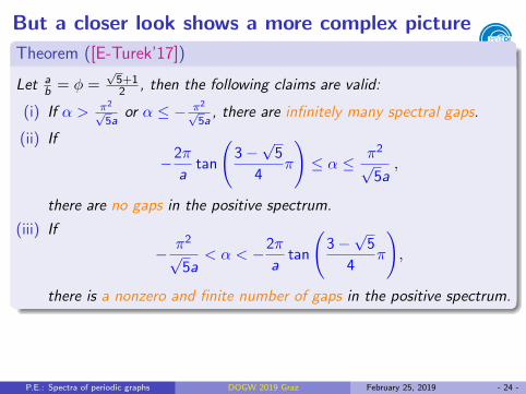
But a closer look shows a more complex picture
Theorem ([E-Turek’17])
Let ab = φ =
√5+12 , then the following claims are valid:
(i) If α > π2√
5aor α ≤ − π2
√5a
, there are infinitely many spectral gaps.
(ii) If
−2π
atan
(3−√
5
4π
)≤ α ≤ π2
√5a,
there are no gaps in the positive spectrum.
(iii) If
− π2
√5a
< α < −2π
atan
(3−√
5
4π
),
there is a nonzero and finite number of gaps in the positive spectrum.
Corollary
The above theorem about the existence of BS graphs is valid.
P.E.: Spectra of periodic graphs DOGW 2019 Graz February 25, 2019 - 24 -

More about this example
The window in which the golden-mean lattice has the Bethe–Sommerfeldproperty is narrow, it is roughly 4.298 . −αa . 4.414.
We are also able to control the number of gaps in the BS regime:
Theorem ([E-Turek’17])
For a given N ∈ N, there are exactly N gaps in the positive spectrum ifand only if α is chosen within the bounds
−2π(φ2(N+1) − φ−2(N+1)
)√
5atan(π
2φ−2(N+1)
)≤ α < −
2π(φ2N − φ−2N
)√
5atan(π
2φ−2N
).
Note that the numbers Aj :=2π(φ2j−φ−2j)√
5tan(π2φ−2j)
form an increasing
sequence the first element of which is A1 = 2π tan(
3−√
54 π
)and
Aj <π2
√5
for all j ∈ N .
P.E.: Spectra of periodic graphs DOGW 2019 Graz February 25, 2019 - 25 -

More general result
Proofs of the above results are based on properties of Diophantineapproximations. In a similar way one can prove
Theorem ([E-Turek’17])
Let θ = ab and define
γ+ := min
{infm∈N
{2mπ
atan(π
2(mθ−1 − bmθ−1c)
)}, infm∈N
{2mπ
btan(π
2(mθ − bmθc)
)}}
and γ− similarly with b·c replaced by d·e. If the coupling constant αsatisfies
γ± < ±α <π2
max{a, b}µ(θ) ,
then there is a nonzero and finite number of gaps in the positive spectrum.
P.E.: Spectra of periodic graphs DOGW 2019 Graz February 25, 2019 - 26 -

More general result
Proofs of the above results are based on properties of Diophantineapproximations. In a similar way one can prove
Theorem ([E-Turek’17])
Let θ = ab and define
γ+ := min
{infm∈N
{2mπ
atan(π
2(mθ−1 − bmθ−1c)
)}, infm∈N
{2mπ
btan(π
2(mθ − bmθc)
)}}
and γ− similarly with b·c replaced by d·e
. If the coupling constant αsatisfies
γ± < ±α <π2
max{a, b}µ(θ) ,
then there is a nonzero and finite number of gaps in the positive spectrum.
P.E.: Spectra of periodic graphs DOGW 2019 Graz February 25, 2019 - 26 -

More general result
Proofs of the above results are based on properties of Diophantineapproximations. In a similar way one can prove
Theorem ([E-Turek’17])
Let θ = ab and define
γ+ := min
{infm∈N
{2mπ
atan(π
2(mθ−1 − bmθ−1c)
)}, infm∈N
{2mπ
btan(π
2(mθ − bmθc)
)}}
and γ− similarly with b·c replaced by d·e. If the coupling constant αsatisfies
γ± < ±α <π2
max{a, b}µ(θ) ,
then there is a nonzero and finite number of gaps in the positive spectrum.
P.E.: Spectra of periodic graphs DOGW 2019 Graz February 25, 2019 - 26 -

Another application of periodic quantum graphs
Square lattice graphs were recently suggested a tool to model theanomalous Hall effect, cf. [Streda-Kucera’15], i.e. the situation when aHall voltage appears without the presence of an external magnetic field
The mechanism giving rise to the effect is not completely clear but it isbelieved that it comes from internal magnetization in combination withthe spin-orbit interaction
To mimick the rotational motion of atomic orbitals responsible for themagnetization, the authors had to impose ‘by hand’ the requirement thatthe electrons move only one way on the loops of the lattice. Naturally,such an assumption cannot be justified from the first principles
This motivated us to investigate situations where such an inherentrotation can take place, not at the graphs edges but in its vertices
P.E.: Spectra of periodic graphs DOGW 2019 Graz February 25, 2019 - 27 -

Another application of periodic quantum graphs
Square lattice graphs were recently suggested a tool to model theanomalous Hall effect, cf. [Streda-Kucera’15], i.e. the situation when aHall voltage appears without the presence of an external magnetic field
The mechanism giving rise to the effect is not completely clear but it isbelieved that it comes from internal magnetization in combination withthe spin-orbit interaction
To mimick the rotational motion of atomic orbitals responsible for themagnetization, the authors had to impose ‘by hand’ the requirement thatthe electrons move only one way on the loops of the lattice
. Naturally,such an assumption cannot be justified from the first principles
This motivated us to investigate situations where such an inherentrotation can take place, not at the graphs edges but in its vertices
P.E.: Spectra of periodic graphs DOGW 2019 Graz February 25, 2019 - 27 -

Another application of periodic quantum graphs
Square lattice graphs were recently suggested a tool to model theanomalous Hall effect, cf. [Streda-Kucera’15], i.e. the situation when aHall voltage appears without the presence of an external magnetic field
The mechanism giving rise to the effect is not completely clear but it isbelieved that it comes from internal magnetization in combination withthe spin-orbit interaction
To mimick the rotational motion of atomic orbitals responsible for themagnetization, the authors had to impose ‘by hand’ the requirement thatthe electrons move only one way on the loops of the lattice. Naturally,such an assumption cannot be justified from the first principles
This motivated us to investigate situations where such an inherentrotation can take place, not at the graphs edges but in its vertices
P.E.: Spectra of periodic graphs DOGW 2019 Graz February 25, 2019 - 27 -

Another application of periodic quantum graphs
Square lattice graphs were recently suggested a tool to model theanomalous Hall effect, cf. [Streda-Kucera’15], i.e. the situation when aHall voltage appears without the presence of an external magnetic field
The mechanism giving rise to the effect is not completely clear but it isbelieved that it comes from internal magnetization in combination withthe spin-orbit interaction
To mimick the rotational motion of atomic orbitals responsible for themagnetization, the authors had to impose ‘by hand’ the requirement thatthe electrons move only one way on the loops of the lattice. Naturally,such an assumption cannot be justified from the first principles
This motivated us to investigate situations where such an inherentrotation can take place, not at the graphs edges but in its vertices
P.E.: Spectra of periodic graphs DOGW 2019 Graz February 25, 2019 - 27 -

The coupling choiceIn the vertex coupling conditions mentioned above,
(U − I )Ψ + i(U + I )Ψ′ = 0 ,
we choose the unitary matrix U of the form
U =
0 1 0 0 · · · 0 0
0 0 1 0 · · · 0 0
0 0 0 1 · · · 0 0
· · · · · · · · · · · · · · · · · · · · ·0 0 0 0 · · · 0 1
1 0 0 0 · · · 0 0
;
the aim is to achieve ‘maximum rotation’ at a fixed energy, conventionallycorresponding the momentum k = 1 . Recall that one has U = S(1)
Componentwise, with ψj = ψj(0+) and ψ′j = ψ′j(0+), we have
(ψj+1 − ψj) + i(ψ′j+1 + ψ′j) = 0 , j ∈ Z (modN) ,
which is non-trivial only for N ≥ 3 and obviously non-invariant w.r.t. thereverse in the edge numbering order
P.E.: Spectra of periodic graphs DOGW 2019 Graz February 25, 2019 - 28 -

The coupling choiceIn the vertex coupling conditions mentioned above,
(U − I )Ψ + i(U + I )Ψ′ = 0 ,
we choose the unitary matrix U of the form
U =
0 1 0 0 · · · 0 0
0 0 1 0 · · · 0 0
0 0 0 1 · · · 0 0
· · · · · · · · · · · · · · · · · · · · ·0 0 0 0 · · · 0 1
1 0 0 0 · · · 0 0
;
the aim is to achieve ‘maximum rotation’ at a fixed energy, conventionallycorresponding the momentum k = 1
. Recall that one has U = S(1)
Componentwise, with ψj = ψj(0+) and ψ′j = ψ′j(0+), we have
(ψj+1 − ψj) + i(ψ′j+1 + ψ′j) = 0 , j ∈ Z (modN) ,
which is non-trivial only for N ≥ 3 and obviously non-invariant w.r.t. thereverse in the edge numbering order
P.E.: Spectra of periodic graphs DOGW 2019 Graz February 25, 2019 - 28 -

The coupling choiceIn the vertex coupling conditions mentioned above,
(U − I )Ψ + i(U + I )Ψ′ = 0 ,
we choose the unitary matrix U of the form
U =
0 1 0 0 · · · 0 0
0 0 1 0 · · · 0 0
0 0 0 1 · · · 0 0
· · · · · · · · · · · · · · · · · · · · ·0 0 0 0 · · · 0 1
1 0 0 0 · · · 0 0
;
the aim is to achieve ‘maximum rotation’ at a fixed energy, conventionallycorresponding the momentum k = 1 . Recall that one has U = S(1)
Componentwise, with ψj = ψj(0+) and ψ′j = ψ′j(0+), we have
(ψj+1 − ψj) + i(ψ′j+1 + ψ′j) = 0 , j ∈ Z (modN) ,
which is non-trivial only for N ≥ 3 and obviously non-invariant w.r.t. thereverse in the edge numbering order
P.E.: Spectra of periodic graphs DOGW 2019 Graz February 25, 2019 - 28 -

The coupling choiceIn the vertex coupling conditions mentioned above,
(U − I )Ψ + i(U + I )Ψ′ = 0 ,
we choose the unitary matrix U of the form
U =
0 1 0 0 · · · 0 0
0 0 1 0 · · · 0 0
0 0 0 1 · · · 0 0
· · · · · · · · · · · · · · · · · · · · ·0 0 0 0 · · · 0 1
1 0 0 0 · · · 0 0
;
the aim is to achieve ‘maximum rotation’ at a fixed energy, conventionallycorresponding the momentum k = 1 . Recall that one has U = S(1)
Componentwise, with ψj = ψj(0+) and ψ′j = ψ′j(0+), we have
(ψj+1 − ψj) + i(ψ′j+1 + ψ′j) = 0 , j ∈ Z (modN) ,
which is non-trivial only for N ≥ 3 and obviously non-invariant w.r.t. thereverse in the edge numbering order
P.E.: Spectra of periodic graphs DOGW 2019 Graz February 25, 2019 - 28 -

Spectrum and on-shell S-matrix
Such a star-graph Hamiltonian H obviously has σess(H) = R+
.Furthermore, it is easy to check thatH has eigenvalues −κ2, where
κ = tanπm
N
with m running through 1, . . . , [N2 ] for N odd and 1, . . . , [N−12 ] for N even.
Thus σdisc(H) is always nonempty, in particular, H has a single negativeeigenvalue for N = 3, 4 which is equal to −1 and −3, respectively
For any vertex coupling U the S-matrix at the momentum k is
S(k) =k − 1 + (k + 1)U
k + 1 + (k − 1)U;
recall that we used U = S(1) when constructing our coupling
It might seem that the transport becomes trivial at small and highenergies, since limk→0 S(k) = −I and limk→∞ S(k) = I
P.E.: Spectra of periodic graphs DOGW 2019 Graz February 25, 2019 - 29 -

Spectrum and on-shell S-matrix
Such a star-graph Hamiltonian H obviously has σess(H) = R+.Furthermore, it is easy to check thatH has eigenvalues −κ2, where
κ = tanπm
N
with m running through 1, . . . , [N2 ] for N odd and 1, . . . , [N−12 ] for N even.
Thus σdisc(H) is always nonempty
, in particular, H has a single negativeeigenvalue for N = 3, 4 which is equal to −1 and −3, respectively
For any vertex coupling U the S-matrix at the momentum k is
S(k) =k − 1 + (k + 1)U
k + 1 + (k − 1)U;
recall that we used U = S(1) when constructing our coupling
It might seem that the transport becomes trivial at small and highenergies, since limk→0 S(k) = −I and limk→∞ S(k) = I
P.E.: Spectra of periodic graphs DOGW 2019 Graz February 25, 2019 - 29 -

Spectrum and on-shell S-matrix
Such a star-graph Hamiltonian H obviously has σess(H) = R+.Furthermore, it is easy to check thatH has eigenvalues −κ2, where
κ = tanπm
N
with m running through 1, . . . , [N2 ] for N odd and 1, . . . , [N−12 ] for N even.
Thus σdisc(H) is always nonempty, in particular, H has a single negativeeigenvalue for N = 3, 4 which is equal to −1 and −3, respectively
For any vertex coupling U the S-matrix at the momentum k is
S(k) =k − 1 + (k + 1)U
k + 1 + (k − 1)U;
recall that we used U = S(1) when constructing our coupling
It might seem that the transport becomes trivial at small and highenergies, since limk→0 S(k) = −I and limk→∞ S(k) = I
P.E.: Spectra of periodic graphs DOGW 2019 Graz February 25, 2019 - 29 -

Spectrum and on-shell S-matrix
Such a star-graph Hamiltonian H obviously has σess(H) = R+.Furthermore, it is easy to check thatH has eigenvalues −κ2, where
κ = tanπm
N
with m running through 1, . . . , [N2 ] for N odd and 1, . . . , [N−12 ] for N even.
Thus σdisc(H) is always nonempty, in particular, H has a single negativeeigenvalue for N = 3, 4 which is equal to −1 and −3, respectively
For any vertex coupling U the S-matrix at the momentum k is
S(k) =k − 1 + (k + 1)U
k + 1 + (k − 1)U;
recall that we used U = S(1) when constructing our coupling
It might seem that the transport becomes trivial at small and highenergies, since limk→0 S(k) = −I and limk→∞ S(k) = I
P.E.: Spectra of periodic graphs DOGW 2019 Graz February 25, 2019 - 29 -

The on-shell S-matrix, continuedHowever, more caution is needed; the formal limits is false if +1 or−1 are eigenvalues of U
. A counterexample is provided by Kirchhoffcoupling where U has only ±1 as its eigenvalues; the correspondingS-matrix is k-independent and not a multiple of the identity
Denoting η := 1−k1+k we get by a straightforward computation
Sij(k) =1− η2
1− ηN{−η 1− ηN−2
1− η2δij + (1− δij) η(j−i−1)(modN)
}This suggests, in particular, that the high-energy behavior, η → −1−,could be determined by the parity of the vertex degree N. Indeed, we seethat limk→∞ S(k) = I holds for N = 3 and more generally for all odd N
On the hand, for N = 4 we have
S(k) =1
1 + η2
−η 1 η η2
η2 −η 1 η
η η2 −η 1
1 η η2 −η
so the limit is not a multiple of identity; the same is true for any even N
P.E.: Spectra of periodic graphs DOGW 2019 Graz February 25, 2019 - 30 -

The on-shell S-matrix, continuedHowever, more caution is needed; the formal limits is false if +1 or−1 are eigenvalues of U. A counterexample is provided by Kirchhoffcoupling where U has only ±1 as its eigenvalues; the correspondingS-matrix is k-independent and not a multiple of the identity
Denoting η := 1−k1+k
we get by a straightforward computation
Sij(k) =1− η2
1− ηN{−η 1− ηN−2
1− η2δij + (1− δij) η(j−i−1)(modN)
}This suggests, in particular, that the high-energy behavior, η → −1−,could be determined by the parity of the vertex degree N. Indeed, we seethat limk→∞ S(k) = I holds for N = 3 and more generally for all odd N
On the hand, for N = 4 we have
S(k) =1
1 + η2
−η 1 η η2
η2 −η 1 η
η η2 −η 1
1 η η2 −η
so the limit is not a multiple of identity; the same is true for any even N
P.E.: Spectra of periodic graphs DOGW 2019 Graz February 25, 2019 - 30 -

The on-shell S-matrix, continuedHowever, more caution is needed; the formal limits is false if +1 or−1 are eigenvalues of U. A counterexample is provided by Kirchhoffcoupling where U has only ±1 as its eigenvalues; the correspondingS-matrix is k-independent and not a multiple of the identity
Denoting η := 1−k1+k we get by a straightforward computation
Sij(k) =1− η2
1− ηN{−η 1− ηN−2
1− η2δij + (1− δij) η(j−i−1)(modN)
}
This suggests, in particular, that the high-energy behavior, η → −1−,could be determined by the parity of the vertex degree N. Indeed, we seethat limk→∞ S(k) = I holds for N = 3 and more generally for all odd N
On the hand, for N = 4 we have
S(k) =1
1 + η2
−η 1 η η2
η2 −η 1 η
η η2 −η 1
1 η η2 −η
so the limit is not a multiple of identity; the same is true for any even N
P.E.: Spectra of periodic graphs DOGW 2019 Graz February 25, 2019 - 30 -

The on-shell S-matrix, continuedHowever, more caution is needed; the formal limits is false if +1 or−1 are eigenvalues of U. A counterexample is provided by Kirchhoffcoupling where U has only ±1 as its eigenvalues; the correspondingS-matrix is k-independent and not a multiple of the identity
Denoting η := 1−k1+k we get by a straightforward computation
Sij(k) =1− η2
1− ηN{−η 1− ηN−2
1− η2δij + (1− δij) η(j−i−1)(modN)
}This suggests, in particular, that the high-energy behavior, η → −1−,could be determined by the parity of the vertex degree N
. Indeed, we seethat limk→∞ S(k) = I holds for N = 3 and more generally for all odd N
On the hand, for N = 4 we have
S(k) =1
1 + η2
−η 1 η η2
η2 −η 1 η
η η2 −η 1
1 η η2 −η
so the limit is not a multiple of identity; the same is true for any even N
P.E.: Spectra of periodic graphs DOGW 2019 Graz February 25, 2019 - 30 -
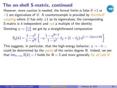
The on-shell S-matrix, continuedHowever, more caution is needed; the formal limits is false if +1 or−1 are eigenvalues of U. A counterexample is provided by Kirchhoffcoupling where U has only ±1 as its eigenvalues; the correspondingS-matrix is k-independent and not a multiple of the identity
Denoting η := 1−k1+k we get by a straightforward computation
Sij(k) =1− η2
1− ηN{−η 1− ηN−2
1− η2δij + (1− δij) η(j−i−1)(modN)
}This suggests, in particular, that the high-energy behavior, η → −1−,could be determined by the parity of the vertex degree N. Indeed, we seethat limk→∞ S(k) = I holds for N = 3 and more generally for all odd N
On the hand, for N = 4 we have
S(k) =1
1 + η2
−η 1 η η2
η2 −η 1 η
η η2 −η 1
1 η η2 −η
so the limit is not a multiple of identity; the same is true for any even N
P.E.: Spectra of periodic graphs DOGW 2019 Graz February 25, 2019 - 30 -

The on-shell S-matrix, continuedHowever, more caution is needed; the formal limits is false if +1 or−1 are eigenvalues of U. A counterexample is provided by Kirchhoffcoupling where U has only ±1 as its eigenvalues; the correspondingS-matrix is k-independent and not a multiple of the identity
Denoting η := 1−k1+k we get by a straightforward computation
Sij(k) =1− η2
1− ηN{−η 1− ηN−2
1− η2δij + (1− δij) η(j−i−1)(modN)
}This suggests, in particular, that the high-energy behavior, η → −1−,could be determined by the parity of the vertex degree N. Indeed, we seethat limk→∞ S(k) = I holds for N = 3 and more generally for all odd N
On the hand, for N = 4 we have
S(k) =1
1 + η2
−η 1 η η2
η2 −η 1 η
η η2 −η 1
1 η η2 −η
so the limit is not a multiple of identity
; the same is true for any even N
P.E.: Spectra of periodic graphs DOGW 2019 Graz February 25, 2019 - 30 -

The on-shell S-matrix, continuedHowever, more caution is needed; the formal limits is false if +1 or−1 are eigenvalues of U. A counterexample is provided by Kirchhoffcoupling where U has only ±1 as its eigenvalues; the correspondingS-matrix is k-independent and not a multiple of the identity
Denoting η := 1−k1+k we get by a straightforward computation
Sij(k) =1− η2
1− ηN{−η 1− ηN−2
1− η2δij + (1− δij) η(j−i−1)(modN)
}This suggests, in particular, that the high-energy behavior, η → −1−,could be determined by the parity of the vertex degree N. Indeed, we seethat limk→∞ S(k) = I holds for N = 3 and more generally for all odd N
On the hand, for N = 4 we have
S(k) =1
1 + η2
−η 1 η η2
η2 −η 1 η
η η2 −η 1
1 η η2 −η
so the limit is not a multiple of identity; the same is true for any even N
P.E.: Spectra of periodic graphs DOGW 2019 Graz February 25, 2019 - 30 -

Comparison of two lattices
00 0
Spectral condition for the cases are easy to derive,
16i ei(θ1+θ2) k sin k`[(k2 − 1)(cos θ1 + cos θ2) + 2(k2 + 1) cos k`
]= 0
and
16i e−i(θ1+θ2 k2 sin k`(
3 + 6k2 − k4 + 4dθ(k2 − 1) + (k2 + 3)2 cos 2k`)
= 0 ,
where dθ := cos θ1 + cos(θ1 − θ2) + cos θ2 , respectively, where1` (θ1, θ2) ∈ [−π
` ,π` ]2 is the quasimomentum, but tedious to solve except
the flat band cases, sin k` = 0
However, we can present the band solution in a graphical form
P.E.: Spectra of periodic graphs DOGW 2019 Graz February 25, 2019 - 31 -

Comparison of two lattices
00 0
Spectral condition for the cases are easy to derive,
16i ei(θ1+θ2) k sin k`[(k2 − 1)(cos θ1 + cos θ2) + 2(k2 + 1) cos k`
]= 0
and
16i e−i(θ1+θ2 k2 sin k`(
3 + 6k2 − k4 + 4dθ(k2 − 1) + (k2 + 3)2 cos 2k`)
= 0 ,
where dθ := cos θ1 + cos(θ1 − θ2) + cos θ2 , respectively, where1` (θ1, θ2) ∈ [−π
` ,π` ]2 is the quasimomentum
, but tedious to solve exceptthe flat band cases, sin k` = 0
However, we can present the band solution in a graphical form
P.E.: Spectra of periodic graphs DOGW 2019 Graz February 25, 2019 - 31 -

Comparison of two lattices
00 0
Spectral condition for the cases are easy to derive,
16i ei(θ1+θ2) k sin k`[(k2 − 1)(cos θ1 + cos θ2) + 2(k2 + 1) cos k`
]= 0
and
16i e−i(θ1+θ2 k2 sin k`(
3 + 6k2 − k4 + 4dθ(k2 − 1) + (k2 + 3)2 cos 2k`)
= 0 ,
where dθ := cos θ1 + cos(θ1 − θ2) + cos θ2 , respectively, where1` (θ1, θ2) ∈ [−π
` ,π` ]2 is the quasimomentum, but tedious to solve except
the flat band cases, sin k` = 0
However, we can present the band solution in a graphical form
P.E.: Spectra of periodic graphs DOGW 2019 Graz February 25, 2019 - 31 -

Picture worth of thousand wordsFor the two lattices, respectively, we get (with ` = 3
2 , dashed ` = 14 )
-5 0 5 10
-1
0
1
2
3
4
and
-5 0 5 10
-1
0
1
2
3
4
P.E.: Spectra of periodic graphs DOGW 2019 Graz February 25, 2019 - 32 -

Picture worth of thousand wordsFor the two lattices, respectively, we get (with ` = 3
2 , dashed ` = 14 )
-5 0 5 10
-1
0
1
2
3
4
and
-5 0 5 10
-1
0
1
2
3
4
P.E.: Spectra of periodic graphs DOGW 2019 Graz February 25, 2019 - 32 -

Comparison of spectral properties
Some features are common:
the number of open gaps is always infinite
the gaps are centered around the flat bands except the lowest one
for some values of ` a band may degenerate
the negative spectrum is always nonempty, the gaps becomeexponentially narrow around star graph eigenvalues as `→∞
But the high energy behavior of these lattices is substantially different:
the spectrum is dominated by bands for square lattices
it is dominated by gaps for hexagonal lattices
Other interesting results can be found, say, concerning interpolationbetween the δ-coupling and the present one. This is our next topic
P.E.: Spectra of periodic graphs DOGW 2019 Graz February 25, 2019 - 33 -

Comparison of spectral properties
Some features are common:
the number of open gaps is always infinite
the gaps are centered around the flat bands except the lowest one
for some values of ` a band may degenerate
the negative spectrum is always nonempty, the gaps becomeexponentially narrow around star graph eigenvalues as `→∞
But the high energy behavior of these lattices is substantially different:
the spectrum is dominated by bands for square lattices
it is dominated by gaps for hexagonal lattices
Other interesting results can be found, say, concerning interpolationbetween the δ-coupling and the present one
. This is our next topic
P.E.: Spectra of periodic graphs DOGW 2019 Graz February 25, 2019 - 33 -

Comparison of spectral properties
Some features are common:
the number of open gaps is always infinite
the gaps are centered around the flat bands except the lowest one
for some values of ` a band may degenerate
the negative spectrum is always nonempty, the gaps becomeexponentially narrow around star graph eigenvalues as `→∞
But the high energy behavior of these lattices is substantially different:
the spectrum is dominated by bands for square lattices
it is dominated by gaps for hexagonal lattices
Other interesting results can be found, say, concerning interpolationbetween the δ-coupling and the present one. This is our next topic
P.E.: Spectra of periodic graphs DOGW 2019 Graz February 25, 2019 - 33 -

More generally on vertex coupling symmetriesA symmetry is described by an invertible map in the space of boundaryvalues, Θ : Cn → Cn. A vertex coupling is symmetric w.r.t Θ if the usualmatching condition is equivalent to
(U − I )ΘΨ(0) + i(U + I )ΘΨ′(0) = 0 ,
or in other words, if U obeys Θ−1UΘ = U
. Some common examples:
Mirror symmetric couplings have the matching conditions invariantagainst (ψ1(0), . . . , ψn(0)) 7→ (ψn(0), . . . , ψ1(0)) and the same forthe derivatives; in other words, Θ = A, the matrix with the entriesequal to 1 on the main antidiagonal and zero otherwiseThe subset of permutation-invariant couplings is a two-parameterfamily, U = aI + bJ, where J denotes the matrix with all the entriesequal to one; the parameters satisfy |a| = 1 and |a + nb| = 1Time-reversal-invariant couplings: in this case Θ is replaced by theantilinear operator of complex conjugation, and using relationsUtU = UUt = I we find easily that the matrix describing thecoupling must be now invariant w.r.t. transposition, U = Ut
P.E.: Spectra of periodic graphs DOGW 2019 Graz February 25, 2019 - 34 -

More generally on vertex coupling symmetriesA symmetry is described by an invertible map in the space of boundaryvalues, Θ : Cn → Cn. A vertex coupling is symmetric w.r.t Θ if the usualmatching condition is equivalent to
(U − I )ΘΨ(0) + i(U + I )ΘΨ′(0) = 0 ,
or in other words, if U obeys Θ−1UΘ = U. Some common examples:
Mirror symmetric couplings have the matching conditions invariantagainst (ψ1(0), . . . , ψn(0)) 7→ (ψn(0), . . . , ψ1(0)) and the same forthe derivatives; in other words, Θ = A, the matrix with the entriesequal to 1 on the main antidiagonal and zero otherwise
The subset of permutation-invariant couplings is a two-parameterfamily, U = aI + bJ, where J denotes the matrix with all the entriesequal to one; the parameters satisfy |a| = 1 and |a + nb| = 1Time-reversal-invariant couplings: in this case Θ is replaced by theantilinear operator of complex conjugation, and using relationsUtU = UUt = I we find easily that the matrix describing thecoupling must be now invariant w.r.t. transposition, U = Ut
P.E.: Spectra of periodic graphs DOGW 2019 Graz February 25, 2019 - 34 -

More generally on vertex coupling symmetriesA symmetry is described by an invertible map in the space of boundaryvalues, Θ : Cn → Cn. A vertex coupling is symmetric w.r.t Θ if the usualmatching condition is equivalent to
(U − I )ΘΨ(0) + i(U + I )ΘΨ′(0) = 0 ,
or in other words, if U obeys Θ−1UΘ = U. Some common examples:
Mirror symmetric couplings have the matching conditions invariantagainst (ψ1(0), . . . , ψn(0)) 7→ (ψn(0), . . . , ψ1(0)) and the same forthe derivatives; in other words, Θ = A, the matrix with the entriesequal to 1 on the main antidiagonal and zero otherwiseThe subset of permutation-invariant couplings is a two-parameterfamily, U = aI + bJ, where J denotes the matrix with all the entriesequal to one; the parameters satisfy |a| = 1 and |a + nb| = 1
Time-reversal-invariant couplings: in this case Θ is replaced by theantilinear operator of complex conjugation, and using relationsUtU = UUt = I we find easily that the matrix describing thecoupling must be now invariant w.r.t. transposition, U = Ut
P.E.: Spectra of periodic graphs DOGW 2019 Graz February 25, 2019 - 34 -

More generally on vertex coupling symmetriesA symmetry is described by an invertible map in the space of boundaryvalues, Θ : Cn → Cn. A vertex coupling is symmetric w.r.t Θ if the usualmatching condition is equivalent to
(U − I )ΘΨ(0) + i(U + I )ΘΨ′(0) = 0 ,
or in other words, if U obeys Θ−1UΘ = U. Some common examples:
Mirror symmetric couplings have the matching conditions invariantagainst (ψ1(0), . . . , ψn(0)) 7→ (ψn(0), . . . , ψ1(0)) and the same forthe derivatives; in other words, Θ = A, the matrix with the entriesequal to 1 on the main antidiagonal and zero otherwiseThe subset of permutation-invariant couplings is a two-parameterfamily, U = aI + bJ, where J denotes the matrix with all the entriesequal to one; the parameters satisfy |a| = 1 and |a + nb| = 1Time-reversal-invariant couplings: in this case Θ is replaced by theantilinear operator of complex conjugation, and using relationsUtU = UUt = I we find easily that the matrix describing thecoupling must be now invariant w.r.t. transposition, U = Ut
P.E.: Spectra of periodic graphs DOGW 2019 Graz February 25, 2019 - 34 -

Symmetries, continued
Our focus here is on rotationally symmetric vertex coupling, i.e. thoseindependent of cyclic permutations of the entries of Ψ(0) and Ψ′(0).They correspond to
Θ = R :=
0 1 0 0 · · · 0 0
0 0 1 0 · · · 0 0
0 0 0 1 · · · 0 0
· · · · · · · · · · · · · · · · · · · · ·0 0 0 0 · · · 0 1
1 0 0 0 · · · 0 0
,
Proposition
A rotationally symmetric vertex coupling is mirror symmetric if and only ifit is time-reversal-invariant.
Note also that while the notions of permutation-invariant and time-reversal-invariant couplings are universal in the sense that they do notrequire embedding in an ambient space, the other two mentioned abovemake sense only if we think of the graph Γ as of an embedded object
P.E.: Spectra of periodic graphs DOGW 2019 Graz February 25, 2019 - 35 -

Circulant matricesMatrices satisfying Θ−1UΘ = U for the above Θ = R are circulantmatrices, which generally take the form
c0 c1 · · · cn−2 cn−1
cn−1 c0 c1 cn−2
.
.
. cn−1 c0
. . ....
c2
. . .. . . c1
c1 c2 · · · cn−1 c0
,
being a particular case of Toeplitz matrices. The first row, i.e. the vectorc = (c0, c1, . . . , cn−1), is called generator of C
Let us recall basic properties of such matrices. The vectors
vk =1√n
(1, ωk , ω2k , . . . , ω(n−1)k
)T, k = 0, 1, . . . , n − 1 ,
with ω := e2πi/n are its normalized eigenvectors corresponding to
λk = c0 + c1ωk + c2ω
2k + · · ·+ cn−1ω(n−1)k , k = 0, 1, . . . , n − 1 .
P.E.: Spectra of periodic graphs DOGW 2019 Graz February 25, 2019 - 36 -

Circulant matrices, continued
Every circulant matrix C is diagonalized by the Discrete Fourier Transformmatrix
F =
1 1 1 1 . . . 1
1 ω ω2 ω3 . . . ωn−1
1 ω2 ω4 ω6 . . . ω2(n−1)
.
.
.
.
.
.
.
.
.
.
.
.
.
.
.
1 ωn−1 ω2(n−1) ω3(n−1) . . . ω(n−1)2
,
in other words, D = 1nF∗CF is a diagonal matrix with λ0, λ1, . . . , λn−1 on
the diagonal. Since F−1 = 1nF∗, we can express from this relation
cj =1
n
(λ0 + λ1ω
−j + λ2ω−2j + · · ·+ λn−1ω
−(n−1)j)
A circulant matrix is unitary if and only if |λj | = 1 holds for all indicesj = 0, 1, . . . , n − 1. Consequently, circulant unitary matrices of order nare parametrized by an n-tuple of real numbers
P.E.: Spectra of periodic graphs DOGW 2019 Graz February 25, 2019 - 37 -

Circulant matrices, continued
Every circulant matrix C is diagonalized by the Discrete Fourier Transformmatrix
F =
1 1 1 1 . . . 1
1 ω ω2 ω3 . . . ωn−1
1 ω2 ω4 ω6 . . . ω2(n−1)
.
.
.
.
.
.
.
.
.
.
.
.
.
.
.
1 ωn−1 ω2(n−1) ω3(n−1) . . . ω(n−1)2
,
in other words, D = 1nF∗CF is a diagonal matrix with λ0, λ1, . . . , λn−1 on
the diagonal
. Since F−1 = 1nF∗, we can express from this relation
cj =1
n
(λ0 + λ1ω
−j + λ2ω−2j + · · ·+ λn−1ω
−(n−1)j)
A circulant matrix is unitary if and only if |λj | = 1 holds for all indicesj = 0, 1, . . . , n − 1. Consequently, circulant unitary matrices of order nare parametrized by an n-tuple of real numbers
P.E.: Spectra of periodic graphs DOGW 2019 Graz February 25, 2019 - 37 -

Circulant matrices, continued
Every circulant matrix C is diagonalized by the Discrete Fourier Transformmatrix
F =
1 1 1 1 . . . 1
1 ω ω2 ω3 . . . ωn−1
1 ω2 ω4 ω6 . . . ω2(n−1)
.
.
.
.
.
.
.
.
.
.
.
.
.
.
.
1 ωn−1 ω2(n−1) ω3(n−1) . . . ω(n−1)2
,
in other words, D = 1nF∗CF is a diagonal matrix with λ0, λ1, . . . , λn−1 on
the diagonal. Since F−1 = 1nF∗, we can express from this relation
cj =1
n
(λ0 + λ1ω
−j + λ2ω−2j + · · ·+ λn−1ω
−(n−1)j)
A circulant matrix is unitary if and only if |λj | = 1 holds for all indicesj = 0, 1, . . . , n − 1. Consequently, circulant unitary matrices of order nare parametrized by an n-tuple of real numbers
P.E.: Spectra of periodic graphs DOGW 2019 Graz February 25, 2019 - 37 -

Circulant matrices, continued
Every circulant matrix C is diagonalized by the Discrete Fourier Transformmatrix
F =
1 1 1 1 . . . 1
1 ω ω2 ω3 . . . ωn−1
1 ω2 ω4 ω6 . . . ω2(n−1)
.
.
.
.
.
.
.
.
.
.
.
.
.
.
.
1 ωn−1 ω2(n−1) ω3(n−1) . . . ω(n−1)2
,
in other words, D = 1nF∗CF is a diagonal matrix with λ0, λ1, . . . , λn−1 on
the diagonal. Since F−1 = 1nF∗, we can express from this relation
cj =1
n
(λ0 + λ1ω
−j + λ2ω−2j + · · ·+ λn−1ω
−(n−1)j)
A circulant matrix is unitary if and only if |λj | = 1 holds for all indicesj = 0, 1, . . . , n − 1. Consequently, circulant unitary matrices of order nare parametrized by an n-tuple of real numbers
P.E.: Spectra of periodic graphs DOGW 2019 Graz February 25, 2019 - 37 -

A class of interpolating couplings
Our aim is now to investigate a class of couplings interpolating betweenthe ‘maximally rotational’ one discussed above and the usual δ couplingreferring to
U = −I +2
n + iαJ ,
where α ∈ R is a parameter; the case α = 0 is called Kirchhoff coupling
We seek a family of unitary matrices {U(t) : t ∈ [0, 1]} such that
U(0) = −I + 2n+iαJ and U(1) = R;
the map t 7→ U(t) is continuous on [0, 1];
U(t) is unitary circulant for all t ∈ [0, 1].
We will construct them using their eigenvalues. For the circulant matrixU(1) we get
λk = ωk if k = 0, 1, . . . , n − 1
P.E.: Spectra of periodic graphs DOGW 2019 Graz February 25, 2019 - 38 -
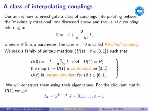

A class of interpolating couplingsSimilarly, the eigenvalues of U(0) are
λk = −1 +2
n + iα
n−1∑j=0
ωjk =
n−iαn+iα for k = 0 ;
−1 for k ≥ 1 .
For brevity, let us set n−iαn+iα = e−iγ ; note that γ
= 0 for α = 0;
∈ (0, π) for α > 0;
∈ (−π, 0) for α < 0.
Then are looking for a matrix with the eigenvalues
λk(t) =
e−i(1−t)γ for k = 0;
−eiπt( 2kn−1) for k ≥ 1
for all t ∈ [0, 1] which would satisfy the stated requirements correspondingto
cj(t) =1
n
(e−i(1−t)γ −
n−1∑k=1
eiπt(2kn−1) · ω−kj
)
P.E.: Spectra of periodic graphs DOGW 2019 Graz February 25, 2019 - 39 -

A class of interpolating couplingsSimilarly, the eigenvalues of U(0) are
λk = −1 +2
n + iα
n−1∑j=0
ωjk =
n−iαn+iα for k = 0 ;
−1 for k ≥ 1 .
For brevity, let us set n−iαn+iα = e−iγ ; note that γ
= 0 for α = 0;
∈ (0, π) for α > 0;
∈ (−π, 0) for α < 0.
Then are looking for a matrix with the eigenvalues
λk(t) =
e−i(1−t)γ for k = 0;
−eiπt( 2kn−1) for k ≥ 1
for all t ∈ [0, 1] which would satisfy the stated requirements
correspondingto
cj(t) =1
n
(e−i(1−t)γ −
n−1∑k=1
eiπt(2kn−1) · ω−kj
)
P.E.: Spectra of periodic graphs DOGW 2019 Graz February 25, 2019 - 39 -

A class of interpolating couplingsSimilarly, the eigenvalues of U(0) are
λk = −1 +2
n + iα
n−1∑j=0
ωjk =
n−iαn+iα for k = 0 ;
−1 for k ≥ 1 .
For brevity, let us set n−iαn+iα = e−iγ ; note that γ
= 0 for α = 0;
∈ (0, π) for α > 0;
∈ (−π, 0) for α < 0.
Then are looking for a matrix with the eigenvalues
λk(t) =
e−i(1−t)γ for k = 0;
−eiπt( 2kn−1) for k ≥ 1
for all t ∈ [0, 1] which would satisfy the stated requirements correspondingto
cj(t) =1
n
(e−i(1−t)γ −
n−1∑k=1
eiπt(2kn−1) · ω−kj
)P.E.: Spectra of periodic graphs DOGW 2019 Graz February 25, 2019 - 39 -

Spectrum of a star graphLet Γ be star with n semi-infinite edges, then it is easy to check thatthe essential/continuous spectrum is [0,∞)
. The negative spectrum isnonempty for any t ∈ (0, 1] and n ≥ 3. Indeed, writing ψj(x) = bje
−κx ,we get the spectral condition
det[(U(t)− I )− iκ(U(t) + I )] = 0 ,
which is equivalent to κ = −i λj (t)−1λj (t)+1 for some 0 ≤ j ≤ n − 1. This yields
κ = − tan(1− t)γ
2for α < 0 and t 6= 1
κ = − cot
(j
n− 1
2
)πt for n ≥ 3 and j < n
2
These solutions give rise to the eigenvalues −κ2 < 0 of the star graph:
there is a negative eigenvalue − tan2 (1−t)γ2 whenever α < 0;
if n ≥ 3, there is an additional bn−12 c-tuple for aech t ∈ (0, 1], namely
− cot2(
jn − 1
2
)πt with j running through 1, . . . , n−1
2 for n odd and
1, . . . , n2 − 1 for n even
P.E.: Spectra of periodic graphs DOGW 2019 Graz February 25, 2019 - 40 -

Spectrum of a star graphLet Γ be star with n semi-infinite edges, then it is easy to check thatthe essential/continuous spectrum is [0,∞). The negative spectrum isnonempty for any t ∈ (0, 1] and n ≥ 3. Indeed, writing ψj(x) = bje
−κx ,we get the spectral condition
det[(U(t)− I )− iκ(U(t) + I )] = 0 ,
which is equivalent to κ = −i λj (t)−1λj (t)+1 for some 0 ≤ j ≤ n − 1
. This yields
κ = − tan(1− t)γ
2for α < 0 and t 6= 1
κ = − cot
(j
n− 1
2
)πt for n ≥ 3 and j < n
2
These solutions give rise to the eigenvalues −κ2 < 0 of the star graph:
there is a negative eigenvalue − tan2 (1−t)γ2 whenever α < 0;
if n ≥ 3, there is an additional bn−12 c-tuple for aech t ∈ (0, 1], namely
− cot2(
jn − 1
2
)πt with j running through 1, . . . , n−1
2 for n odd and
1, . . . , n2 − 1 for n even
P.E.: Spectra of periodic graphs DOGW 2019 Graz February 25, 2019 - 40 -

Spectrum of a star graphLet Γ be star with n semi-infinite edges, then it is easy to check thatthe essential/continuous spectrum is [0,∞). The negative spectrum isnonempty for any t ∈ (0, 1] and n ≥ 3. Indeed, writing ψj(x) = bje
−κx ,we get the spectral condition
det[(U(t)− I )− iκ(U(t) + I )] = 0 ,
which is equivalent to κ = −i λj (t)−1λj (t)+1 for some 0 ≤ j ≤ n − 1. This yields
κ = − tan(1− t)γ
2for α < 0 and t 6= 1
κ = − cot
(j
n− 1
2
)πt for n ≥ 3 and j < n
2
These solutions give rise to the eigenvalues −κ2 < 0 of the star graph:
there is a negative eigenvalue − tan2 (1−t)γ2 whenever α < 0;
if n ≥ 3, there is an additional bn−12 c-tuple for aech t ∈ (0, 1], namely
− cot2(
jn − 1
2
)πt with j running through 1, . . . , n−1
2 for n odd and
1, . . . , n2 − 1 for n evenP.E.: Spectra of periodic graphs DOGW 2019 Graz February 25, 2019 - 40 -

Eigenvalue limiting behavior
Finally, look at what the eigenvalues do in the limits t → 0+ (δ coupling)
and t → 1− (the ‘extreme’ rotational coupling):
If t → 0+, all the eigenvalues −κ2 diverge to −∞ except for− tan2 (1−t)γ
2 occurring for α < 0, which approaches the value− tan2(γ/2) = −α2/n2. When t = 0, the ‘additional’ eigenvaluesthus disappear and the system has only one simple negative eigenvalue−α2/n2 for α < 0, while for α ≥ 0 its negative spectrum is empty
If t → 1−, the eigenvalues −κ2 approach zero and − tan2 jn ,
respectively. When t = 1, the only negative eigenvalues are − tan2 jn
with j taking values 1, . . . , n−12 for n odd and 1, . . . , n2 − 1 for n even
– as we have seen before
P.E.: Spectra of periodic graphs DOGW 2019 Graz February 25, 2019 - 41 -

Eigenvalue limiting behavior
Finally, look at what the eigenvalues do in the limits t → 0+ (δ coupling)and t → 1− (the ‘extreme’ rotational coupling):
If t → 0+, all the eigenvalues −κ2 diverge to −∞ except for− tan2 (1−t)γ
2 occurring for α < 0, which approaches the value− tan2(γ/2) = −α2/n2
. When t = 0, the ‘additional’ eigenvaluesthus disappear and the system has only one simple negative eigenvalue−α2/n2 for α < 0, while for α ≥ 0 its negative spectrum is empty
If t → 1−, the eigenvalues −κ2 approach zero and − tan2 jn ,
respectively. When t = 1, the only negative eigenvalues are − tan2 jn
with j taking values 1, . . . , n−12 for n odd and 1, . . . , n2 − 1 for n even
– as we have seen before
P.E.: Spectra of periodic graphs DOGW 2019 Graz February 25, 2019 - 41 -

Eigenvalue limiting behavior
Finally, look at what the eigenvalues do in the limits t → 0+ (δ coupling)and t → 1− (the ‘extreme’ rotational coupling):
If t → 0+, all the eigenvalues −κ2 diverge to −∞ except for− tan2 (1−t)γ
2 occurring for α < 0, which approaches the value− tan2(γ/2) = −α2/n2. When t = 0, the ‘additional’ eigenvaluesthus disappear and the system has only one simple negative eigenvalue−α2/n2 for α < 0, while for α ≥ 0 its negative spectrum is empty
If t → 1−, the eigenvalues −κ2 approach zero and − tan2 jn ,
respectively. When t = 1, the only negative eigenvalues are − tan2 jn
with j taking values 1, . . . , n−12 for n odd and 1, . . . , n2 − 1 for n even
– as we have seen before
P.E.: Spectra of periodic graphs DOGW 2019 Graz February 25, 2019 - 41 -

Eigenvalue limiting behavior
Finally, look at what the eigenvalues do in the limits t → 0+ (δ coupling)and t → 1− (the ‘extreme’ rotational coupling):
If t → 0+, all the eigenvalues −κ2 diverge to −∞ except for− tan2 (1−t)γ
2 occurring for α < 0, which approaches the value− tan2(γ/2) = −α2/n2. When t = 0, the ‘additional’ eigenvaluesthus disappear and the system has only one simple negative eigenvalue−α2/n2 for α < 0, while for α ≥ 0 its negative spectrum is empty
If t → 1−, the eigenvalues −κ2 approach zero and − tan2 jn ,
respectively
. When t = 1, the only negative eigenvalues are − tan2 jn
with j taking values 1, . . . , n−12 for n odd and 1, . . . , n2 − 1 for n even
– as we have seen before
P.E.: Spectra of periodic graphs DOGW 2019 Graz February 25, 2019 - 41 -

Eigenvalue limiting behavior
Finally, look at what the eigenvalues do in the limits t → 0+ (δ coupling)and t → 1− (the ‘extreme’ rotational coupling):
If t → 0+, all the eigenvalues −κ2 diverge to −∞ except for− tan2 (1−t)γ
2 occurring for α < 0, which approaches the value− tan2(γ/2) = −α2/n2. When t = 0, the ‘additional’ eigenvaluesthus disappear and the system has only one simple negative eigenvalue−α2/n2 for α < 0, while for α ≥ 0 its negative spectrum is empty
If t → 1−, the eigenvalues −κ2 approach zero and − tan2 jn ,
respectively. When t = 1, the only negative eigenvalues are − tan2 jn
with j taking values 1, . . . , n−12 for n odd and 1, . . . , n2 − 1 for n even
– as we have seen before
P.E.: Spectra of periodic graphs DOGW 2019 Graz February 25, 2019 - 41 -

ScatteringKnowing U(t) we easily find the on-shell S-matrix. In particular, itseigenvalues are
µj(t) =k − 1 + (k + 1)λj(t)
k + 1 + (k − 1)λj(t)for j = 0, 1, . . . , n − 1.
We are again interested in the high-energy behavior of the S-matrix:
If n is odd, then limk→∞ µj = 1 for all j = 0, 1, . . . , n − 1, hence
limk→∞
S(k) = I
If n is even, then limk→∞ µj = 1 for j 6= n2 , while limk→∞ µn/2 = −1,
and consequently, the generator of limk→∞ S(k) equals(1− 2
n,
2
n,−2
n,
2
n, . . . ,−2
n,
2
n
)As in the ‘extreme’ rotational case, the S-matrix behaves at high energiesdifferently for odd and even n
P.E.: Spectra of periodic graphs DOGW 2019 Graz February 25, 2019 - 42 -
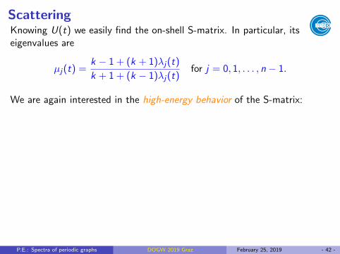

Square latticeWe consider again a lattice of spacing `, now with the interpolatingcoupling. The treatment is similar to the particular case analyzed earlier;it yields the spectral condition
512 ei(θ1+θ2) e−i(1−t)γ
2[V3k
3 + V2k2 + V1k + V0
]= 0 ,
where
V3 = − cos(1− t)γ
2sin2 πt
4sin k`(cos θ1 + cos θ2 + 2 cos k`) ;
V2 = 2 sin(1− t)γ
2sin2 πt
4(cos θ1 + cos k`)(cos θ2 + cos k`) ;
V1 = cos(1− t)γ
2cos2 πt
4sin k`(cos θ1 + cos θ2 − 2 cos k`) ;
V0 = −2 sin(1− t)γ
2cos2 πt
4sin2 k` .
Hence k2 belongs to the spectrum iff there are θ1, θ2 ∈ [−π, π) such that
V3k3 + V2k
2 + V1k + V0 = 0 .
P.E.: Spectra of periodic graphs DOGW 2019 Graz February 25, 2019 - 43 -
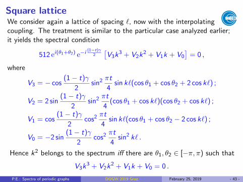

The case α = 0
If α = 0 we have V2 = V0 = 0 and the spectral condition reduces to
sin k`
[(k2 sin2 πt
4− cos2 πt
4
)(cos θ1 + cos θ2)− 2
(k2 sin2 πt
4+ cos2 πt
4
)cos k`
]= 0 .
It has two types of solutions. The first are infinitely degenerateeigenvalues, squares of
mπ
`for m ∈ N .
The condition describing spectral bands can rewritten as∣∣∣k2 sin2 πt
4− cos2 πt
4
∣∣∣ ≥ (k2 sin2 πt
4+ cos2 πt
4
)| cos k`| .
Note that if t = 0 (i.e., pure Kirchhoff), the condition simplifies to| cos k`| ≤ 1, which is satisfied for all k ≥ 0. Putting this trivial caseaside, from now on we assume that t ∈ (0, 1].
P.E.: Spectra of periodic graphs DOGW 2019 Graz February 25, 2019 - 44 -

The case α = 0, continued
For t ∈ (0, 1] the spectrum obviously contains infinitely many gaps locatedin the vicinity of k = mπ
` for m ∈ N. The band condition for k > 0 can berewritten as(
k
∣∣∣∣tank`
2
∣∣∣∣− cotπt
4
)(k
∣∣∣∣cotk`
2
∣∣∣∣− cotπt
4
)≥ 0
and the zeros of the factors correspond to the band edges
. The latterintersect at points where k
∣∣tan k`2
∣∣ = k∣∣cot k`
2
∣∣ = cot πt4 , i.e., at (t, k)such that
k =
(m − 1
2
)π
`and t =
4
πarccot
(m − 1
2
)π
`, m ∈ N .
At those values of t the spectrum shrinks into a ‘flat band’
P.E.: Spectra of periodic graphs DOGW 2019 Graz February 25, 2019 - 45 -

The case α = 0, continued
For t ∈ (0, 1] the spectrum obviously contains infinitely many gaps locatedin the vicinity of k = mπ
` for m ∈ N. The band condition for k > 0 can berewritten as(
k
∣∣∣∣tank`
2
∣∣∣∣− cotπt
4
)(k
∣∣∣∣cotk`
2
∣∣∣∣− cotπt
4
)≥ 0
and the zeros of the factors correspond to the band edges. The latterintersect at points where k
∣∣tan k`2
∣∣ = k∣∣cot k`
2
∣∣ = cot πt4 , i.e., at (t, k)such that
k =
(m − 1
2
)π
`and t =
4
πarccot
(m − 1
2
)π
`, m ∈ N .
At those values of t the spectrum shrinks into a ‘flat band’
P.E.: Spectra of periodic graphs DOGW 2019 Graz February 25, 2019 - 45 -

The case α = 0, continued
0 0.2 0.4 0.6 0.8 1
t
-50
0
50
100
150
E
Figure: Interpolation with the Kirchhoff coupling for ` = 1, the spectrum isindicated by the shaded regions.
P.E.: Spectra of periodic graphs DOGW 2019 Graz February 25, 2019 - 46 -

The case α = 0, continued
The negative spectrum is found in a similar way
. The presence/absence ofa gap above/below zero depends on t, the switch occurs at t = 4
πarctan`2
Let us look at the high-energy behavior of gaps. The condition reads∣∣∣∣(1 +2
k2cot2 πt
4+O(k−4)
)cos k`
∣∣∣∣ > 1 as k →∞
so it can be satisfied only for k located in small neighborhoods of mπ` . The
approximate width of the m-th spectral gap is equal to
4
mπcot
πt
4+O(m−2)
in the momentum variable, hence in energy the gaps are asymptoticallyconstant, of the widths 8
` cot πt4 +O(m−1). Note that the gap widthincreases as t diminishes from this extreme value but eventually it startsto decrease again, to the point of vanishing at t = 0.
P.E.: Spectra of periodic graphs DOGW 2019 Graz February 25, 2019 - 47 -

The case α = 0, continued
The negative spectrum is found in a similar way. The presence/absence ofa gap above/below zero depends on t, the switch occurs at t = 4
πarctan`2
Let us look at the high-energy behavior of gaps. The condition reads∣∣∣∣(1 +2
k2cot2 πt
4+O(k−4)
)cos k`
∣∣∣∣ > 1 as k →∞
so it can be satisfied only for k located in small neighborhoods of mπ` . The
approximate width of the m-th spectral gap is equal to
4
mπcot
πt
4+O(m−2)
in the momentum variable, hence in energy the gaps are asymptoticallyconstant, of the widths 8
` cot πt4 +O(m−1). Note that the gap widthincreases as t diminishes from this extreme value but eventually it startsto decrease again, to the point of vanishing at t = 0.
P.E.: Spectra of periodic graphs DOGW 2019 Graz February 25, 2019 - 47 -
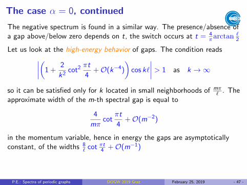
The case α = 0, continued
The negative spectrum is found in a similar way. The presence/absence ofa gap above/below zero depends on t, the switch occurs at t = 4
πarctan`2
Let us look at the high-energy behavior of gaps. The condition reads∣∣∣∣(1 +2
k2cot2 πt
4+O(k−4)
)cos k`
∣∣∣∣ > 1 as k →∞
so it can be satisfied only for k located in small neighborhoods of mπ` . The
approximate width of the m-th spectral gap is equal to
4
mπcot
πt
4+O(m−2)
in the momentum variable, hence in energy the gaps are asymptoticallyconstant, of the widths 8
` cot πt4 +O(m−1)
. Note that the gap widthincreases as t diminishes from this extreme value but eventually it startsto decrease again, to the point of vanishing at t = 0.
P.E.: Spectra of periodic graphs DOGW 2019 Graz February 25, 2019 - 47 -

The case α = 0, continued
The negative spectrum is found in a similar way. The presence/absence ofa gap above/below zero depends on t, the switch occurs at t = 4
πarctan`2
Let us look at the high-energy behavior of gaps. The condition reads∣∣∣∣(1 +2
k2cot2 πt
4+O(k−4)
)cos k`
∣∣∣∣ > 1 as k →∞
so it can be satisfied only for k located in small neighborhoods of mπ` . The
approximate width of the m-th spectral gap is equal to
4
mπcot
πt
4+O(m−2)
in the momentum variable, hence in energy the gaps are asymptoticallyconstant, of the widths 8
` cot πt4 +O(m−1). Note that the gap widthincreases as t diminishes from this extreme value but eventually it startsto decrease again, to the point of vanishing at t = 0.
P.E.: Spectra of periodic graphs DOGW 2019 Graz February 25, 2019 - 47 -
The general case, α ∈ RThe analysis follows the same line but becomes more complicated;the spectral condition now yields spectra, as functions of t, in the formof a union of pairs of regions
Let us summarize our observations about the band spectra of our lattices:
(i) A ‘discontinuity’ at t = 0: There is always a spectral band whichbecomes narrow and strongly negative as t → 0 and eventuallydisappears. This obviously corresponds to the behavior of the‘additional’ eigenvalues of a single vertex
(ii) Point degeneracies for α = 0: In the Kirchhoff case spectral bandsmay collapse to a point at particular values of t. It is not the case ifα 6= 0 where the spectral condition has other solutions which smearthese Kirchhoff degenerate eigenvalues into bands of nonzero width,more pronounced as we are going farther from the Kirchhoff case
(iii) Non-monotonicity of the gap widths: As mentioned already thewidths of the gaps are not monotonous with respect to theinterpolation parameter, the same is true if α 6= 0
P.E.: Spectra of periodic graphs DOGW 2019 Graz February 25, 2019 - 48 -

Illustration, weakly attractive interaction
0 0.2 0.4 0.6 0.8 1
t
-20
-10
0
10
20
30
40
E
Figure: Interpolation with an attractive δ coupling, α = −4(√
2− 1), ` = 1.
P.E.: Spectra of periodic graphs DOGW 2019 Graz February 25, 2019 - 49 -

Illustration, strongly attractive interaction
0 0.2 0.4 0.6 0.8 1
t
-20
-10
0
10
20
30
40
E
Figure: Interpolation with an attractive δ coupling, α = −4(√
2 + 1), ` = 1.
P.E.: Spectra of periodic graphs DOGW 2019 Graz February 25, 2019 - 50 -

Other properties
(iv) α-independence of some bands: Some curves marking the bandedges are independent of α. However, for α 6= 0 the ‘band edges’coincide only in parts of the interval [0, 1], as there is a neighborhoodof t = 4
πarccot3π2 in which there is an additional spectrum
(v) ‘Band edge’ regularity: The curves delineating the band edges aredescribed by analytic functions. In the Kirchhoff case the analyticityis violated only at the points when the curves are crossing, on theother hand, in the case α 6= 0 where the spectrum is a union of bandsthere are other points where each particular edge is not smooth;needless to say, it remains Lipshitz
(vi) Flat band spreading: Infinitely degenerate eigenvalues for t = 1 maysmear when the interpolation parameter decreases, but we know thatthey also remain in the spectrum. A possible explanation may comefrom the presence of different ‘elementary’ eigenfunctions in the caset = 1, namely ‘Dirichlet’ and ‘Neumann’ type, which could behavedifferently with respect to t
P.E.: Spectra of periodic graphs DOGW 2019 Graz February 25, 2019 - 51 -

Illustration, larger lattice spacing
0 0.2 0.4 0.6 0.8 1
t
-1.5
-1
-0.5
0
0.5
1
1.5
2
2.5
E
Figure: Interpolation with an attractive δ coupling, α = −4(√
2 + 1) and l = 2π.
P.E.: Spectra of periodic graphs DOGW 2019 Graz February 25, 2019 - 52 -

And finally, band edges positionsLooking for extrema of the dispersion functions, people usually seekthem and the border of the respective Brillouin zone
As a warning, [Harrison-Kuchment-Sobolev-Winn’07] constructed exampleof a periodic quantum graph in which (some) band edges correspond tointernal points of the Brillouin zone
Subsequently, in [E-Kuchment-Winn’10] it was shown that same may betrue even for graphs periodic in one dimension
The number of connecting edges had to be N ≥ 2. An example:
P.E.: Spectra of periodic graphs DOGW 2019 Graz February 25, 2019 - 53 -

And finally, band edges positionsLooking for extrema of the dispersion functions, people usually seekthem and the border of the respective Brillouin zone
As a warning, [Harrison-Kuchment-Sobolev-Winn’07] constructed exampleof a periodic quantum graph in which (some) band edges correspond tointernal points of the Brillouin zone
Subsequently, in [E-Kuchment-Winn’10] it was shown that same may betrue even for graphs periodic in one dimension
The number of connecting edges had to be N ≥ 2
. An example:
P.E.: Spectra of periodic graphs DOGW 2019 Graz February 25, 2019 - 53 -

And finally, band edges positionsLooking for extrema of the dispersion functions, people usually seekthem and the border of the respective Brillouin zone
As a warning, [Harrison-Kuchment-Sobolev-Winn’07] constructed exampleof a periodic quantum graph in which (some) band edges correspond tointernal points of the Brillouin zone
Subsequently, in [E-Kuchment-Winn’10] it was shown that same may betrue even for graphs periodic in one dimension
The number of connecting edges had to be N ≥ 2. An example:
P.E.: Spectra of periodic graphs DOGW 2019 Graz February 25, 2019 - 53 -

Band edges, continued
In the same paper we showed that if N ≥ 2, the band edges correspondto periodic and antiperiodic solutions
However, we did it under that assumption that the system is invariantw.r.t. time reversal. To show that this assumption was essential considera comb-shaped graph with our non-invariant coupling at the vertices
r r r r r r r r r rIts analysis shows:
two-sided comb is transport-friendly, bands dominate
one-sided comb is transport-unfriendly, gaps dominate
sending the one side edge lengths to zero in a two-sided combdoes not yield one-sided comb transport
and what about the dispersion curves?
P.E.: Spectra of periodic graphs DOGW 2019 Graz February 25, 2019 - 54 -
Band edges, continued
In the same paper we showed that if N ≥ 2, the band edges correspondto periodic and antiperiodic solutions
However, we did it under that assumption that the system is invariantw.r.t. time reversal
. To show that this assumption was essential considera comb-shaped graph with our non-invariant coupling at the vertices
r r r r r r r r r rIts analysis shows:
two-sided comb is transport-friendly, bands dominate
one-sided comb is transport-unfriendly, gaps dominate
sending the one side edge lengths to zero in a two-sided combdoes not yield one-sided comb transport
and what about the dispersion curves?
P.E.: Spectra of periodic graphs DOGW 2019 Graz February 25, 2019 - 54 -

Band edges, continued
In the same paper we showed that if N ≥ 2, the band edges correspondto periodic and antiperiodic solutions
However, we did it under that assumption that the system is invariantw.r.t. time reversal. To show that this assumption was essential considera comb-shaped graph with our non-invariant coupling at the vertices
r r r r r r r r r rIts analysis shows:
two-sided comb is transport-friendly, bands dominate
one-sided comb is transport-unfriendly, gaps dominate
sending the one side edge lengths to zero in a two-sided combdoes not yield one-sided comb transport
and what about the dispersion curves?
P.E.: Spectra of periodic graphs DOGW 2019 Graz February 25, 2019 - 54 -

Band edges, continued
In the same paper we showed that if N ≥ 2, the band edges correspondto periodic and antiperiodic solutions
However, we did it under that assumption that the system is invariantw.r.t. time reversal. To show that this assumption was essential considera comb-shaped graph with our non-invariant coupling at the vertices
r r r r r
r r r r rIts analysis shows:
two-sided comb is transport-friendly, bands dominate
one-sided comb is transport-unfriendly, gaps dominate
sending the one side edge lengths to zero in a two-sided combdoes not yield one-sided comb transport
and what about the dispersion curves?
P.E.: Spectra of periodic graphs DOGW 2019 Graz February 25, 2019 - 54 -

Band edges, continued
In the same paper we showed that if N ≥ 2, the band edges correspondto periodic and antiperiodic solutions
However, we did it under that assumption that the system is invariantw.r.t. time reversal. To show that this assumption was essential considera comb-shaped graph with our non-invariant coupling at the vertices
r r r r r r r r r r
Its analysis shows:
two-sided comb is transport-friendly, bands dominate
one-sided comb is transport-unfriendly, gaps dominate
sending the one side edge lengths to zero in a two-sided combdoes not yield one-sided comb transport
and what about the dispersion curves?
P.E.: Spectra of periodic graphs DOGW 2019 Graz February 25, 2019 - 54 -

Band edges, continued
In the same paper we showed that if N ≥ 2, the band edges correspondto periodic and antiperiodic solutions
However, we did it under that assumption that the system is invariantw.r.t. time reversal. To show that this assumption was essential considera comb-shaped graph with our non-invariant coupling at the vertices
r r r r r r r r r rIts analysis shows:
two-sided comb is transport-friendly, bands dominate
one-sided comb is transport-unfriendly, gaps dominate
sending the one side edge lengths to zero in a two-sided combdoes not yield one-sided comb transport
and what about the dispersion curves?
P.E.: Spectra of periodic graphs DOGW 2019 Graz February 25, 2019 - 54 -

Band edges, continued
In the same paper we showed that if N ≥ 2, the band edges correspondto periodic and antiperiodic solutions
However, we did it under that assumption that the system is invariantw.r.t. time reversal. To show that this assumption was essential considera comb-shaped graph with our non-invariant coupling at the vertices
r r r r r r r r r rIts analysis shows:
two-sided comb is transport-friendly, bands dominate
one-sided comb is transport-unfriendly, gaps dominate
sending the one side edge lengths to zero in a two-sided combdoes not yield one-sided comb transport
and what about the dispersion curves?
P.E.: Spectra of periodic graphs DOGW 2019 Graz February 25, 2019 - 54 -

Two-sided comb: dispersion curves
−3 −2 −1 0 1 2 3
θ
0.0
0.5
1.0
1.5
2.0
2.5
3.0
3.5
4.0
P.E.: Spectra of periodic graphs DOGW 2019 Graz February 25, 2019 - 55 -

The sources
The examples discussed in this talk come from
[EV17] P.E., Daniel Vasata: Cantor spectra of magnetic chain graphs, J. Phys. A:Math. Theor. 50 (2017), 165201 (13pp)
[ET17a] P.E., Ondrej Turek: Quantum graphs with the Bethe-Sommerfeld property,Nanosystems 8 (2017), 305–309.
[ET17b] P.E., Ondrej Turek: Periodic quantum graphs from the Bethe-Sommerfeldpoint of view, J. Phys. A: Math. Theor. 50 (2017), 455201 (32pp)
[ET18] P.E., M.Tater: Quantum graphs with vertices of a preferred orientation, Phys. Lett.A382 (2018), 283–287.
[ETT18] P.E., O.Turek, M.Tater: A family of quantum graph vertex couplings interpolatingbetween different symmetries, J. Phys. A: Math. Theor. 51 (2018), 285301 (22pp)
[EV19] P.E., Daniel Vasata: Spectral properties of Z periodic quantum chains without timereversal invariance, in preparation
in combination the other papers mentioned in the course of thepresentation.
P.E.: Spectra of periodic graphs DOGW 2019 Graz February 25, 2019 - 56 -

It remains to say
Thank you for your attention!
P.E.: Spectra of periodic graphs DOGW 2019 Graz February 25, 2019 - 57 -

It remains to say
Thank you for your attention!
P.E.: Spectra of periodic graphs DOGW 2019 Graz February 25, 2019 - 57 -
![Coarse grained spectra, dynamics and quantum phase space ... · orbits of the system, Bogomolny [173 and Berry [18] have shown the effect of localization on unstable periodic orbits](https://img.pdfslide.us/doc/110x75/5e04c660f6972c5b825f4300/coarse-grained-spectra-dynamics-and-quantum-phase-space-orbits-of-the-system.jpg)


![PERIODIC CLASSIFICATION & PERIODIC PROPERTIES [ 1 ...youvaacademy.com/youvaadmin/image/PERIODIC TABLE BY RS.pdf · [ 2 ] PERIODIC CLASSIFICATION & PERIODIC PROPERTIES BY RAJESH SHAH](https://img.pdfslide.us/doc/110x75/604570870a43592d4f6b3e29/periodic-classification-periodic-properties-1-table-by-rspdf-2.jpg)