Embed Size (px)
Citation preview

wik-Consult • Report
Specification Report for the Australian Competition and Consumer Commission
Specification of the strategic network planning
tool GSM-CONNECT for implementing the WIK-MNCM
Bad Honnef, May 2007

WIK-Consult GmbH does not accept any responsibility and disclaims all liability (including negligence) for the consequences of any person (individuals, companies, public bodies etc.) other than the Australian Competition and Consumer Commission acting or refraining from acting as a result of the contents of this specification.

GSM-CONNECT Specification I
Contents
List of Figures and Tables III
List of Abbreviations and Terms IV
List of Authors VII
1 Introduction 1
2 GSM network architecture services and data aggregation 2
2.1 GSM network architecture 2
2.2 Second generation services considered in the WIK-MNCM 4
2.3 Data collection for a nationwide GSM network in Australia 5
3 Functional specification 7
3.1 Scenario Creator 7
3.2 Cell deployment 10
3.3 Aggregation network 16
3.3.1 Algorithm for the B-CLASIG problem 18
3.3.2 Algorithm for the BSCTREE problem 24
3.3.3 Algorithm for the RO&RAL-ASIG problem 27
3.4 Backhaul network 29
3.5 Core network 30
3.6 Parameter values for various scenarios 39
3.6.1 Parameter values for the cell deployment 40
3.6.2 Parameter values for the aggregation network configuration 41
3.6.3 Parameter values for the backhaul and core network configuration 46
4 Data file specification 50
4.1 Cell deployment input data files specification 50
4.1.1 Output files 55
4.1.2 File for the evaluation of the results 59
4.2 Aggregation network data file specification 59
4.2.1 Output files 60
4.2.2 Files for the evaluation of the results 63
4.3 Backhaul network data file specification 64
4.3.1 Input files 64

II GSM-CONNECT Specification
4.3.2 Output files 65
4.3.3 Files for the evaluation of the results 66
4.4 CORE-DESIGN data file specification 67
4.4.1 Input files 67
4.4.2 Output files 67
4.4.3 Files for evaluating the results 70
Annex I: Consideration of traffic values in the local BH of a District and in the global BH in a MSC due to user mobility 71
Annex II: Study for the physical layer of a core network 73
References 77

GSM-CONNECT Specification III
List of Figures and Tables
Figure 2-1 Architecture of a GSM network 2
Figure 3-1 Projection of the real extension of a District to an equivalent circular geographical extension 11
Figure 3-2 Cell size determination process 13
Figure 3-3 Example of the BSCTREE corresponding to a BSC cluster with its corresponding external PTPRAL 18
Figure 3-4 GSM architecture and its corresponding interconnection points 31
Figure 3-5 Example for the traffic distribution and routing for On-Net traffic: A) Traffic pattern after routing, B) Traffic distribution pattern 33
Figure 3-6 Time differences in Australia a) time zones during Standard Time
relative to Greenwich Mean Time, b) time zones during Summer Time relative to Greenwich Mean Time 35
Figure 3-7 Values of resilience and cost parameters as a function of the number of BSCs 43
Figure 3-8 Values of increase/decrease characteristic parameters for the BSCTREE as a function of the penalty value 45
Figure 3-9 Values of composite parameters (length and hops; length and flow) as a function of the penalty value 46
Figure 3-10 Cost per minute and average traffic load (expressed by the number of users) as a function of the number of MSCs 47
Figure 3-11 Core network topology for the 25 per cent scenario 48
Table 2-1 Nomenclature of the network hierarchy of the GSM network model 4
Table 3-1 The SNPT service set with its corresponding input values 16

IV GSM-CONNECT Specification
List of Abbreviations and Terms
2G Second generation or Global System for Mobile Communications 3G Third generation, is the generic term used for the next generation of
mobile communications systems ACCC Australian Competition and Consumer Commission ANSI American National Standards Institute ATM Asynchronous Transfer Mode B Basic BCLASIG BSC Assignation/Assignment BH Busy Hour BN Backhaul Network Bottom-Up A cost modelling approach that models the network and cost structures
of a hypothetical operator. This efficient operator employs modern technology and is not constrained by technology, systems and architectural decisions of the past. A bottom-up model identifies all components of the network necessary to produce the services in question. Based on engineering and economic experience and evidence, cost causation relationships are then defined to link the relevant quantities of outputs with network components and other relevant cost drivers.
BSC Base Station Controller BSCTREE Base Station Controller Tree BSC-BSC link Link between one BSC and another BSC BSC-BTS link Link between a BSC and a BTS BSC-MSC link Link between a BSC and a MSC BSS Base Station Subsystem BTS Base Transmission Station BTS hub Centrally located BTS in a District with the largest traffic flow BTS hub-BSC Link between BTS hub and a BSC Busy Hour The period in a day experiencing peak network traffic volume CDMA Code Division Multiple Access CN Core Network CORE-DESIGN A component of the core network module. The CORE-DESIGN task is
divided into two parts: the first one is the logical design which ends with determining the required number of STM-1 DSGs which connect the different MSC locations. The second part, named physical design, involves the determination of the corresponding physical topology, which connects the MSC locations, the routing of the STM-1 DSG demand on this topology and finally the determination of the transmission systems and medias.
CWDM Coarse Wave Division Multiplex CWLP Capacitated Warehouse Location Problem dB Decibel DFSA Deepest First Search Algorithm DiLeL Digital Leased Lines District Aggregated postal areas based on population and physical size. Districts
are the basic geographical unit used for calculating cell deployment.

GSM-CONNECT Specification V
DLL Dynamic Link Library. The concept of DLL allows to separate the user interface and the calculation algorithms in the software development. Therefore changes in one part do not affect the other part, and hence it allows an efficient reuse of the software in new applications.
DS1 ANSI framing specification for the transmission of 24 64 Kbps data streams
DSG Digital Signal Group DWDM Dense Wave Division Multiplex E1 ETSI framing specification for the transmission of 32 64 Kbps data
streams ETSI European Telecommunications Standards Institute FL-LRIC Forward Looking Long Run Incremental Cost FWC Fixed Wired Circuits GoS Grade of Service GPRS General Packet Radio Service GSM Global System for Mobile Communications GWU Gateway Unit HSCSDS High Speed Circuit Switched Data Service ISDN Integrated Services Digital Network IT Information Technology ITU International Telecommunication Union Kbps Kilobits Per Second LRIC Long Run Incremental Cost mErl Milli Erlang Mbps Megabits Per Second MHz Megahertz MMS Multimedia Message Service MSC Mobile Switching Centre MST Minimal Spanning Tree MTAS Mobile Terminating Access Service NSS Network Switching Subsystem OC Optical Carrier PSTN Public Switched Telephone Network PTP Point to point PTPRAL Point to Point Radio Link QoS Quality of Service SDH Synchronous Digital Hierarchy SMS Short Message Service SNPT Strategic Network Planning Tool STM-1 Synchronous Transfer Module – 1 TDMA Time Division Multiple Access TRAU Transcoder and Rate Adaptation Unit TRX Transceivers W Watts

VI GSM-CONNECT Specification
WIK WIK-Consult WIK-MNCM WIK-Mobile Network and Cost Model

GSM-CONNECT Specification VII
List of Authors
Prof. Dr. Klaus D. Hackbarth Full Professor and Head of the Group for Telematic Engineering at the University of Cantabria, Santander, Spain
Prof. Dr. Antonio Portilla Figueras Associate Professor and Communications Group Coordinator of Signal & Communication Theory, University of Alcalá de Henares, Madrid, Spain
Prof. Dr. Sancho Salcedo-Sanz Associate Professor and Head of the Research Group for Signal & Communication Theory, University of Alcalá de Henares, Madrid, Spain
Laura Rodríguez de Lope López Research Engineer and PhD student in the Group for Telematic Engineering at the University of Cantabria, Santander, Spain
Fernando Fresno-Cambre Master Student at the University of Alcalá de Henares, Madrid, Spain
Carlos Aza-Villarubia Master Student at the University of Alcalá de Henares, Madrid, Spain


GSM-CONNECT Specification 1
1 Introduction
The network design module of the WIK Mobile Network Cost Model (WIK-MNCM) is implemented in the form of a Strategic Network Planning Tool (SNPT).1 This specification document provides a detailed insight into its functions and algorithms and their form of implementation for the user of the WIK-MNCM. For this purpose, the document is divided into five sections: the first section provides a short introduction to the problem of network planning and its application to cost studies. The second section outlines the GSM-Network architecture used in the specification of the WIK-MNCM. The third section provides the specification of the different algorithms, and the fourth section reports the data structure used inside of GSM-CONNECT. Finally, the fifth section summarises the implementation aspects of these issues as relevant to the WIK-MNCM.
The WIK-MNCM is based on a Total Service Long Run Incremental Cost (TSLRIC) framework implemented in the form of Total Service Long Run Element Cost.(TELRIC) The objective of the SNPT is to provide the key engineering inputs for the strategic decisions in the design of a second generation (2G) mobile network, using a Global System for Mobile Communications (GSM) architecture. It estimates results for a given telecommunication network using a bottom-up approach.2 The main application of bottom-up telecommunication network models is that they allow regulators to derive estimates of the efficient cost for a particular country for call termination and interconnection costs.
1 This tool is independently also known as GSM-Connect, as developed by the group around Prof. Hackbarth.
2 For details of bottom-up models in telecommunications regulation in general see Gonzalez et al (2002) and for mobile networks in particular see Hackbarth et al (2005).

2 GSM-CONNECT Specification
2 GSM network architecture services and data aggregation
Section 2.1, provides a description of the GSM network architecture and outlines the issues to be considered when implementing a cost model such as the WIK-MNCM. Section 2.2 lists the most important services supported by a GSM network architecture, including the relevant parameters describing these services, and indicates typical values for these parameters. Section 2.3 describes the method applied to carry out the data aggregation used to configure the national GSM network for a hypothetical GSM network operator in Australia.
2.1 GSM network architecture
In contrast to fixed networks, a bottom-up model for the design of a national GSM network (in the sense of strategic network planning undertaken by a hypothetical new entrant network operator) needs to consider certain issues, because of the use of radio links in the network. The network design and configuration for a mobile operator also depends on the general characteristics or profile of an operator (service portfolio, market share, coverage requirements, and its equipment provider), and demographic and geographic parameters (population, type of terrain, building concentration and so on). A critical design parameter is the technology and the network hierarchy. Figure 2-1 shows the reference architecture of a GSM network.
Figure 2-1 Architecture of a GSM network

GSM-CONNECT Specification 3
This architecture consists of two main levels:
i. The Base Station Subsystem (BSS) and
ii. The Network Switching Subsystem (NSS).
The two main parts of the network are further subdivided into two other levels. The BSS is divided into a radio access part, between the mobile stations (MSs) and the Base Station Transceivers (BTSs), and the aggregation network that connects the BTSs with the Base Station Controllers (BSCs). This aggregation network is often implemented using point-to-point radio links (PTPRALs) using a tree network topology with a BSC as the root location of the tree, where all assigned BTSs start from and terminate to. In some cases fixed wired digital circuits (FWCs) are applied for connections from the BTSs in high density areas, such as metropolitan areas and cities. The BTSs in Districts where no BSC is located may be connected directly to an aggregation point. The connection of all these BTSs form an internal star topology inside the relevant District, and the aggregation point is then connected via an external tree network to the assigned BSC. Figure 3-3 in section 3.2 illustrates an example of this. The SNPT uses a tree network with an optimal mix of PTPRALs and digital leased lines (DiLeLs) provided by Digital Signal Groups (DSGs).
The BSC is the connection point between the BSS and the NSS. Links between the BTSs and the BSCs transport voice, data and signalling traffic through a 16 Kbps slotted structure. The slotted structure of the links is a result of the basic-frame unit of the transceiver (TRX) of the BTS which comprises 8 slots. The bandwidth of these slots is extended inside the NSS to the bandwidth of ISDN digital circuits of 64 Kbps (DS0) and aggregated in the form of standard signalling groups (E1 under ETSI standard and DS1 under ANSI standard). The transformation from the 16 Kbps slots into the 64 Kbps is provided by the Trans-coding Rate Adaptation Unit (TRAU). The TRAU is generally located at the MSC, but in some cases at the BSC. As a consequence, the standard digital groups E1 or DS1 can be connected from the BSC to the MSC by standard DiLeLs as FWCs in the form of a star topology. The underlying network topology of the leased lines system is, in general, a ring with self-healing features. Therefore it provides network resilience for 99.99 per cent of the time. In some cases, a leased line operator can improve the resilience to 99.999 per cent of the time.
The connections between the MSCs are mostly provided by a fully meshed structure of DiLeLs. As an alternative, infrastructure in the form of various interconnected rings (less meshed topology) can also be used. In this specification report, the sub-level of the NSS between the BSC and the MSC is referred to as the 'backhaul network', while the network between the MSCs is known as the ‘core network’. Table 2-1 summarises different aspects of this nomenclature.

4 GSM-CONNECT Specification
Table 2-1 Nomenclature of the network hierarchy of the GSM network model
Network part Sublevel Sub-connection Bandwidth of basic unit Topology
BSS Cell BS-BTS 16 ---
Aggregation BTS-BSC 16 Tree-star
NSS Backhaul BSC-MSC 64 Star or ring
Core MSC-MSC 64 Meshed
2.2 Second generation services considered in the WIK-MNCM
Second generation systems, and more specifically the GSM system, were primarily developed to provide voice services. Therefore, all planning efforts were oriented to providing the corresponding Quality of Service (QoS) and Grade of Service (GoS) for voice services. However, message services such as Short Message Services (SMSs) or even low speed data services such as 9.6 Kbps circuit switched modem services have become increasingly relevant for 2G networks. As an intermediate step before the introduction of 3G services, in the late nineteen nineties, packet data services became very important in the delivery of 2.5G services and the General Packet Radio Services (GPRSs). For this reason, the model includes a broad service portfolio which uses 2G network elements and has evolved from circuit switched services towards packet data services. In fact the model considers the following services:
I. On-Net Voice Service: Voice services between two mobile subscribers within the operator’s network,
II. Off-Net Incoming Voice Service: Voice calls made by a subscriber of another network (fixed or mobile) terminating on the operator's network,
III. Off-Net Outgoing Voice Service: Voice calls made by a subscriber on the operator's network terminating on another network (fixed or mobile),
IV. Basic Data Modem Service: Circuit Switched Data service at a rate of 9.6 Kbps using a single slot,
V. High Speed Circuit Switched Data (HSCSD): Circuit Switched data using several time slots,
VI. SMS: A very popular service with an increasing relevance in mobile networks,
VII. GPRS: Also known as 2.5G, it is the most commonly used method to transmit data in Time Division Multiple Access (TDMA) networks, and

GSM-CONNECT Specification 5
VIII. Multimedia Message Service (MMS): The natural extension of the SMS with pictures and sound. It uses GPRS as the transmission system.
2.3 Data collection for a nationwide GSM network in Australia
An important point in the modelling exercise is the process of collecting relevant data about the geography and demography of the country. This is particularly relevant in countries like Australia, where long distances between the different localities and the degree of distributed population are two important characteristics.
Australia specific information is extracted from public sources about the following:
• Postal Areas in Australia,3
• Data about the Australian geography,4
• Data about Australia’s working population,5 and
• Data about transient population such as travellers.
These data are used to generate the input parameters that are used to estimate the cell deployment for the network in the WIK-MNCM.
From the above data sources the following data categories are generated:
I. Postal Area (POA) code,
II. POA name,
III. POA residential population,
IV. Number of employees and travellers that are temporarily in particular POAs,
V. Area of POAs in square kilometres,
VI. Classification of population density (urban / suburban / rural), and
VII. Topographic features.
Note that the objective of the cell deployment is to determine the number of network resources (sites, BTSs, TRXs) required in a District (which is the relevant service area
3 For details and reference see section 5.1.1 of the Report. 4 For details and reference see section 5.1.5 of the Report. 5 For details and reference see section 5.1.3 of the Report.

6 GSM-CONNECT Specification
used for dimensioning in the WIK-MNCM). POA information is adapted to derive Districts.
Conversion of POAs to Districts may result in exclusion of some uneconomic POAs. Such an area would be an isolated area with a population below a predetermined threshold where it would not be commercially justified to provide services. In these POAs the network deployment is not performed.6
6 As shown later, there may be some low density areas that are nevertheless being served because they become part of larger Districts for which deployment is overall commercially justified.
GSM-CONNECT Specification 7
3 Functional specification
This section provides the specification of the algorithms applied in GSM-CONNECT. From the point of view of software engineering, the information provided about the algorithms is valid independently of the programming language applied and data structure concepts used for its implementation. Hence the functional specification can be understood without any program language knowledge. The section is divided into four sections which correspond to the four key GSM network parts defined in section 2 and shown in Table 2-1.
3.1 Scenario Creator
The objective of the software GSM Scenario Creator is to generate part of the input information for the cell deployment process. Specifically, starting from the general database of the 2,415 Postal Areas with their corresponding information, the GSM Scenario Creator generates a list of Districts ranging from a single POA to a set of POAs joined together using the aggregation rules explained below.
The GSM Scenario Creator has two procedures to obtain the Districts from the list of the POAs:
• Aggregation: POAs that meet certain criteria (expressed in terms of population density thresholds and distance of centres from each other) are aggregated to obtain a single District.
• Exclusion: POAs with population below a specified threshold will not be included. These POAs are uneconomic areas and therefore the operator will not perform any network deployment.
Both procedures are highly interdependent and therefore are explained together.
The starting point is a file containing the list of POAs and relevant information. POAs are ordered according to density of the population and classified based on this density as urban, suburban or rural POAs. It should be noted that ‘population’ means here the ’modified population’ consisting of residents as well as transient (mostly working) people, as derived below.
The key POA information (as outlined above) includes:
• Name of the POA,
• Area in square kilometres,
• Residential population,

8 GSM-CONNECT Specification
• Number of employees and other transient population information such as travellers,
• Type (Urban, Suburban, Rural), and
• Percentage of terrain that can be considered as flat/hilly/mountainous.
The first step consists of the calculation of the modified population for each POA, using the following expression:
( )⎥⎦⎤
⎢⎣⎡ −
⋅+=sinhabitantTotal
employeesTotalinhabitansTotalsinhabitantPOAemployeesPOAsinhabitantPOAMaxsinhabitantPOA_mod
_
____,__
where Total_inhabitants and Total_employees are the sum of the population and the employees respectively, over all POAs.
Once this value is calculated, and in the case where the Exclusion Option is selected, the program runs through the complete list of POAs and compares the population (employees and residents) in each POA with the exclusion threshold that is specified by the user. In case that this population is below the exclusion threshold, the POA is marked as a area which may be potentially excluded from the scenario. Note that at this stage a POA is only tagged for exclusion, it is not excluded until the aggregation process is complete.7
If the Aggregation Option is selected it executes the aggregation procedure which works as follows. The list of POAs is ordered according to the modified population density. The algorithm starts with the POA with the highest modified population density. Having identified a POA the procedure uses the modified population density to select the aggregation radius. If the density is above the maximum threshold it will use the maximum threshold aggregation radius and aggregate all the POAs within that radius (measured in kilometres) to the selected POA. If the density of the selected POA is between the medium and maximum thresholds the procedure will use the medium aggregation radius. If it is below the medium threshold, the procedure will use the minimum aggregation radius. If it is lower than the minimum threshold, this POA will not be aggregated to other POAs.8 Once the selected POA is aggregated into a District, the procedure selects the next non-aggregated POA with the highest population density to continue the aggregation process. Carrying out the procedure in this order ensures that POAs that are aggregated have at most the same order of classification as the POA to
7 If the user of the WIK MNCM does not activate the aggregation process then all POAs tagged for exclusion will be excluded from the cell deployment process.
8 Note that the minimum threshold used in the aggregation process can be set lower than the exclusion threshold.

GSM-CONNECT Specification 9
which they are aggregated (where urban is the highest and rural the lowest classification) and have a lower population density if they are of the same classification.
To illustrate the aggregation process, the following example is used:
Modified Population of POA: 750
Thresholds Inhabitant density Aggregation radius (Km)
Minimum 100 0
Medium 500 10
Maximum 1000 5
In this example, the POA will aggregate other surrounding POAs within a radius of 10 kilometres. Furthermore, a POA to be aggregated to this POA will have a population density below 750 inhabitants/Km2, as the algorithm always starts the aggregation process by selecting a POA with the highest modified population density.
When a POA is aggregated to a District, it is tagged in order to avoid that this POA is aggregated with other POAs in future iterations of the algorithm. After each aggregation step, the algorithm stores a new District in a newly created list, i.e. the District List. This process is continued until all POAs have been checked. Note that with this procedure not all POAs will necessarily be aggregated (independent of whether they are tagged for exclusion or not). There may be large rural POAs which become Districts by themselves since they do not meet the criteria for aggregation in terms of population and distance thresholds.
The next step is to generate the final version of the District List. For this the program reviews the list of POAs that are flagged to be excluded (if the Exclusion Option is on). If such a POA is flagged as 'aggregated' the algorithm ignores it (since it is already part of a District). If the POA is flagged for exclusion and has not been flagged for aggregation, it is excluded from the District List. All POAs not flagged as aggregated but having large enough populations are added to the District List. Finally, all the Districts in the District List arrived at by this procedure are stored in the “Australia_cities.txt” file.

10 GSM-CONNECT Specification
3.2 Cell deployment
The cell deployment is the first and the fundamental step in the design and dimensioning of any mobile network. It is based on the geographical location of population centres (cities, towns etc) and the different services implemented by the operator.
The cell deployment needs to reflect the characteristics of the different Districts. A realistic cell deployment oriented to a real implementation of the network is a resource intensive task and requires the use of Geographical Information Systems (GISs), which contain detailed information about the different types of areas, topography, buildings, etc. The outcome of this type of study is the determination of the exact location of actual BTSs for deployment. It is straightforward to see that this kind of planning is not within the scope of the SNPT for this engagement.

GSM-CONNECT Specification 11
Note that the main input data for the SNPT is the District List (in the Australia_cities.txt file), as described in section 3.1. The term District may refer to a division of a city (consisting of multiple Districts), town or a small rural centre. Note also that the SNPT deals equally with a District of a large city and a small locality. The SNPT introduces the concept of an equivalent area where the whole District is mapped into an equivalent ring area within the same geographical area as the actual area. The SNPT considers the subdivision of the District into three zones – urban, suburban and rural – and assumes that the user density and the other characteristics are consistent within each zone, see Figure 3-1. As a consequence the cell size in each zone is the same and the SNPT has only to calculate three cell radii for each District, one for each zone.9 The number of BTS sites for each zone is then obtained by dividing the geographical extension of the zone by the area covered by a BTS site. Note that this BTS layout does not necessarily reflect real BTS locations; for example it is assumed that a BTS hub is located in the centre of the district while for the other BTSs it is not necessary to specify their locations as their distances to the hub are always assumed to be below the maximum range of a mini link.
Figure 3-1 Projection of the real extension of a District to an equivalent circular geographical extension
(a) real extension of the District (b) circular projection
The parameters for each District in the Australia_cities.txt file include
• Total number of inhabitants,
9 Note that this process is performed for each BTS type specified in the scenario. Each BTS is defined by its transmission power, number of channels, sectoring degree and so on. Therefore if, for example, there are three types of BTS, nine calculations of the cell radius will be performed. The final BTS will be the one which requires the lower number of sites to provide the required coverage and quality of service (QoS) to the zone under study.

12 GSM-CONNECT Specification
• Total geographical extension (Km2) / Radius of the extension (Km),
• Geographical coordinates of the District (central point) in (X,Y) UTM units,
• Type of topography classified into three categories, flat, hilly, mountainous,
• Classifications for density (urban, suburban and rural) and topography (flat, hilly, mountainous),
• Percentage of the geographical extension for each zone in the District, and
• Percentage of the inhabitants for each zone in the District.
In each zone (urban, suburban, rural), the WIK-MNCM needs to estimate the cell radius for each type of BTS considered in the scenario. The cell size determination process is outlined in Figure 3-2.

GSM-CONNECT Specification 13
Figure 3-2 Cell size determination process

14 GSM-CONNECT Specification
As shown in Figure 3-2, the process is repeated for each District, for each zone within the District and for each type of BTS. The first calculation relates to the first band radius by propagation and traffic limits. Depending on the sectorisation input parameters for the BTS applied in the corresponding zone, the deployment is done with or without sectoring. Note that if the BTS is traffic driven, sectoring may result in a larger cell range. If the resulting propagation radius is less than the traffic radius, the deployment has found a solution. If the propagation radius is larger than the traffic radius, the process continues. Now the model checks whether the second band is available for the network deployment. If not, the cell is traffic driven and hence the cell range is the radius calculated by traffic. Otherwise, the model considers that a second band BTS is installed at the same site and hence the model has to calculate its cell range using the same methods as in the case of the first band including sectoring if possible. Then, the minimum value of the radius is chosen as the final one for the second band BTS. With this radius, the program calculates the equivalent population served by the second band BTS. Obviously, this process causes a reduction of the population that has to be served by the first band BTS. Then the traffic radius for the remaining population in the first band is calculated. The program selects between the traffic radius and the propagation radius of the first band previously calculated. Note that these values will be used for the calculation of the number of sites in the corresponding zone of the District.
For the cell calculation, the SNPT requires data input about the traffic generated by the different services offered by the mobile network. These services are classified as circuit-based and packet-based. The bandwidth required for the circuit-based services is expressed as the number of basic units used, where each basic unit corresponds to a slot of the TRX frame. The bandwidth required for packet-based services is expressed as the number of basic units resulting in the corresponding bandwidth, the busy-hour (BH) call rate for using the packet service, the mean duration of the packet service connection and the mean number of packets sent during a connection and its mean length. Table 3-1 shows the different types of services considered and the typical values for its parameters applied. The traffic generated by the circuit switched service is then expressed by the product of the calling rate, the duration of the call and the number of basic units. The traffic unit for a packet service has to reflect the same type of traffic unit as for a circuit switched service.
The Erlang traffic values in the BH which are relevant for network design and dimensioning are derived on the basis of the formulae shown below. These formulae transform the service-specific BH calling rates into equivalent BH Erlang (ρi):
ρVoice = VoiceBH_calling_rate*ts/3600
ρBasic Data = Basic_DataBH_calling_rate*ts /3600

GSM-CONNECT Specification 15
ρSMS = SMSBH_calling_rate*Lp*8*/(bW*3600)
ρHSCSDS = HSCSDBH_calling_rate*ts*nb/3600
ρGPRS = GPRSBH_calling_rate Lp*8*np/(bW*3600)
ρMMS = MMSBH_calling_rate*Lp*8/(bW*3600)
where
ts = call or connection duration (in seconds); i.e. the time the user has an active connection or call, called ‘service time’ or ’channel holding time’
Lp = parameter expressed in bytes which defines the length of the user plane message in case of the MMS and SMS services and the length of the GPRS application layer packet in case of the GPRS service
nb = the number of basic units; i.e. the number of time slots in the GSM TDMA radio access frame which the service uses
np = the average number of user plane packets in each GPRS connection; i.e. the amount of information (measured in packets) the end user needs to transmit
bW = binary rate of the service measured in Kbits per second, where the values depend on the service type defined in the GSM specification

16 GSM-CONNECT Specification
Table 3-1 shows the resulting values of BH traffic as well as the assumed values of the relevant parameters.
Table 3-1 The SNPT service set with its corresponding input values
Service BH
calling rate
Call duration
ts (sec)
Average packet or message
length Lp
(bytes)
Number of basic units
nb
Average packets per connection
np
bW (bps)
BH traffic (milli Erlang
= Erlang*1,000)
Voice On Net 0.077619 87 1.8758
Outgoing Off Net Voice 0.122611 87 2.9631
Incoming Off Net Voice 0.122611 87 2.9631
Basic Data 0.00332 180 0.1660
SMS 0.31533 125 9,600 0.0091
HSCSDS 0.000693 180 2 0.0693
GPRS 0.011205 50 4,000 20,000 0.2490
MMS 0.068475 600 20,000 0.0046
Total 8.3000
The BH Erlang values shown in the table will, for costing purposes, be projected into corresponding annual minutes.
3.3 Aggregation network
As shown in section 2, the GSM aggregation network comprises the network from the BTS to the BSC. To model this part of the network the results from the cell deployment calculation (i.e. the total number of BTSs that are generated based upon the District List and the BH Erlang) are used. For each District the cell deployment provides the number of BTSs, the corresponding traffic and the required number of TRX frames with the corresponding slots. Some Districts will be selected as the location of BSCs. BSCs are assumed to be centrally located in the same location as the BTS site in a District. Each District must now be assigned to a (generally the nearest) BSC. This assignment, will

GSM-CONNECT Specification 17
generally be determined with reference to the shortest geographical distance, but could be assigned to another one if the nearest BSC already has a minimum or maximum number of BTSs assigned. The BSC cluster is the formation derived by assigning each District to a corresponding BSC. The algorithm used to classify and assign BSCs to BTSs is abbreviated by the term B-CLASIG.
Once the B-CLASIG problem is solved, the network connecting each BTS from the Districts to its corresponding BSC needs to be designed. This network structure is represented by a tree structure using either a PTPRAL system or FWCs (e.g. in the form of DiLeLs of E1 digital groups). The name of the relevant algorithm to be solved is represented by BSCTREE. The outcome of the cell deployment process results in Districts being characterised by a central location and surrounded by three concentric rings (classified as urban, suburban, and rural zones). A number of BTSs are located within each ring. Hence, the SNPT does not provide an exact location for each individual BTS, but a representation of these locations within the ring structure. Consistent with an actual network structure, solving the BSCTREE algorithm results in a hierarchical structure composed of a two level tree structure:
i. The internal connection of a BTS within a District to the central point of that District (either at the BSC location in that particular District or an aggregation point (or BTS hub) which is interconnected with a BSC in another District). From a cost point of view, the optimal way to implement this type of connection is to use a type of PTPRAL named Minilink. Using this assumption, the network structure results in a star structure from each BTS to the corresponding aggregation point at the BTS hub.
ii. Note that most Districts will not have a BSC. The aggregation points in these Districts or BTS hubs will be connected to the BSC. This connection is assumed to be through a FWC connection directly to the BSC or by a PTPRAL either directly to its corresponding BSC or over a chain of PTPRALs between Districts. Figure 3-3 illustrates this concept.

18 GSM-CONNECT Specification
Figure 3-3 Example of the BSCTREE corresponding to a BSC cluster with its corresponding external PTPRAL
BSC location (with the corresponding central point of a BTS district)
BTS location
External radio link system or leased line DSG
Internal radio link system
Central point of a BTS district (with a BTS)
Once the tree structure for each BSC cluster is determined, the model has to route the circuit demand from the individual BTS sites to the central node of the District and then the accumulated circuit demand of the District to the corresponding BSC. Once the aggregated circuit demand is known, a radio link system needs to be determined for a PTPRAL connection, this problem is named RO&RAL-ASIG (or the Route and Radio link assignment).
Thus, the network design for the GSM aggregation network has to solve three problems B-CLASIG, BSCTREE and RO&RAL-ASIG.
3.3.1 Algorithm for the B-CLASIG problem
As already outlined, the B-CLASIG problem is divided into two interrelated issues: the selection of higher level nodes (or the BSC sites) from a list of lower level nodes (or BTS sites) and the assignment of those lower level nodes (BTSs) to higher level nodes (BSCs) factoring in capacity constraints. These capacity limits are expressed by the number of BTSs assigned to a corresponding BSC within a range of a feasible (maximum and minimum) number of BTSs that can be assigned to a BSC. Problems of this kind arise in many applications and are generally known as the ‘Capacitated

GSM-CONNECT Specification 19
Warehouse Location Problem’ (CWLP) or in telecommunications as the ‘capacitated concentrator problem.’ The corresponding solution finds the optimal number of BSCs and for every BSC, the optimal number of BTSs factoring in the fixed costs associated with installation (for BSCs) and the variable cost for the links between a BTS and a BSC. As the original problem is Non-Polynomial complex (NP complex) and hence difficult to solve), corresponding algorithms relevant to the size of problems prevalent in real world applications range from traditional ADD&Drop-Interchange heuristics10 to sophisticated optimisation heuristics.11
There are several differences between the B-CLASIG approach used in the WIK-MNCM and the standard formulation of the CWLP:
i. The number of BSCs is not to be optimised but generally predetermined by the network planner as an input parameter,12
ii. The assignment is for Districts with a number of BTSs connected to the BTS hub and not for individual BTSs so that all BTSs connected to the BTS hub are assigned to the relevant BSC,
iii. The cost of connecting a BTS, within a District and from a BTS hub from another District to the relevant BSC, is not linear and depends on the number of radio link (RAL) sections over which the circuit demand is routed and the type of PTPRAL or FWC which will be assigned according to the traffic or circuit demand aggregated to a BTS, and
iv. There are a large number of BTSs and corresponding Districts reflecting a concrete national network, typical figures range from 5,000 to 20,000 for BTSs and 500 to 2000 for Districts.
The first issue (i) results in the so called p-median problem which can be solved as a reduced CWLP, the second issue (ii) creates limits for the assignment solution in relation to capacity constraints, the third issue (iii) shows that the B-CLASIG, BSCTREE and RO&RAL-ASIG problems are correlated and the cost function is not linear. The last issue (iv) relates to the objective of a strategic planning tool which has to consider various scenarios and indicates that a complex heuristic algorithm should not be considered so that long processing times are avoided and the number of calculated and evaluated scenarios is limited.
For these reasons, the SNPT uses a linear heuristic based on a deepest first search algorithm (DFSA) for solving the the BSC selection problem. The assignment solution
10 See Domschke (1990). 11 See Han (2003), pp. 597-618. 12 In telecommunication network design problems the number of nodes inside of a hierarchic level is
determined mainly by technical problems and not by costing models.

20 GSM-CONNECT Specification
minimises the sum of the geographical distance in the assignment of the BTS Districts, starting from an unlimited capacity assignment using the shortest distance criterion. The capacity limits are then applied and using an iterative algorithm the re-assignment problem is solved, where an adaptation in the direction of fulfilling upper capacity limits interchanges with an adaptation in the direction of fulfilling lower capacity limits. An additional parameter limits the Districts which are candidates for this re-assignment procedure to neighbouring Districts using a threshold value (thdist) limiting distance from the BSC to which they were originally assigned. This value is iteratively increased (by a parameter ε) until the re-assignation satisfies the upper and lower BTS limits.
The main procedure is as follows:
B-CLASIG Input data and parameter :
ni list of District nodes (i=1…N with N number of District nodes) δi number of BTS assigned to the District i M number of BSC locations Δmax maximum number of BTS assignable to a BSC Δmin minimum number of BTS assignable to a BSC ε distance increment factor for re-assignation dmin minimum distance between BSCs
Internal variables:
ni Districts without BSC (i=1….N-M) vi Districts with BSC (i= 1…M) C(vi) set of Districts assigned to the BSC vi Δi number of BTS assigned to the BSC i (including the BTSs in the proper District of
the BSC) δi number of BTS assigned to the District i dij distance between ni and vj
Subfunctions : Clustering Selects from the set of District nodes (N) the M nodes for locating the BSCs,
resulting vm (m=1…M) and ni (i=1… N-M) Free-Assig Assigns each ni to the nearest vm, resulting Δm and δm Grad-red makes a re-assignation of a District ni from its BSC vsup to another BSC vk for
reducing the maximum degree Δsup Grad-inc makes a re-assignation of a District ni from its BSC vm to another BSC vinf for
increasing the minimum degree Δinf

GSM-CONNECT Specification 21
Main-Procedure : Clustering Free-assig thdist= ε if solution is feasible (for all vi, Δmin <Δi <Δmax )then feasible =1 else feasible =0 Do while feasible =0 { mejinc=1 Do while mejinc=1 or mejred=1 { mejred=0 Set Vm list in decreasing order of Δm Do over Vm while mejred=0 mejred= Grad-red (Vm, thdist) mejinc=0 Set Vm list in increasing order of Δm Do over Vm while mejinc=0 mejinc= Grad-inc (Vm, thdist) } if solution is feasible then feasible=1 else thdist += ε }

22 GSM-CONNECT Specification
The different sub-functions called by the main procedure are defined as follows:
Clustering (Sub-function in the B-CLASIG procedure)
Input and output parameter
Internal variable : nbsc number of selected BSCs
Procedure : Set ni Districts in decreasing order of δi
select n1 as BSC V1 nbsc=1 Do over all ni (i=2...N) while nbsc <M If distance from ni to selected BSCs ≥ dmin { nbsc++ select ni as BSC Vnbsc } If nbsc < M Error
Free_assig (Sub-function called by the B-CLASIG procedure) Input and output parameter : ni lower nodes (I =1…N-M) vm upper nodes (m =1… M) Internal variable Procedure Do over all ni (i=1...N-M) { assign ni to the nearest upper node vm C(vm) += {ni} Δm+= Δi }

GSM-CONNECT Specification 23
Grad-red (Sub-function called by the B-CLASIG procedure)
Input and output parameter
Internal variable
Procedure : Grad-red (vm, thdist) { find ni ∈C(vm) with δi max /
i) ∃vk / Δk +δi < Δm
ii) thdistl
ll
m,i
m,ik,i ≤−
if solution exists then {
C(vm) -= {ni} ; Δm -= δi C(vk) +={ni} ; Δk += δi mejred=1
} else mejred=0 return mejred }
Grad-inc (Sub-function called by the B-CLASIG procedure)
Input and output parameter
Internal variable
Procedure : Grad-inc (vm, thdist) { find ni ∈C(vk) with δi max /
iii) ∃vk / Δk -δi > Δm
iv) thdistl
ll
k,i
k,im,i ≤−

24 GSM-CONNECT Specification
if solution exists then {
C(vm) += {ni} ; Δm += δi C(vk) -={ni} ; Δk -= δi mejred=1
} else mejred=0 return mejred }
3.3.2 Algorithm for the BSCTREE problem
Given a set of nodes, a tree topology is a network topology which does not contain any cycle and there exists, in general, a large number of different trees. In the case of the BSCTREE problem, an optimal-tree topology is the one which minimises the cost for its implementation. These costs are driven by two main parameters, the capacity required on a link of the tree and the length of a link. The minimum cost network structure when considering the capacity criterion in isolation results in a star topology so that each BTS hub is connected with its corresponding BSC location by routing circuit demand over only one link. On the other hand the minimum cost outcome considering the length criterion results in a tree which minimises the length called minimal spanning tree (MST). The optimal tree used in the WIK-MNCM and calculated from the SNPT for each BSC location considers both criteria. If the PTPRAL systems are more expensive than the DSG leased line solution, the resulting topology will be a star network. However, this is not generally the case because the PTPRALs usually consider the bridges required between the sender and the receiver edges and are therefore not length dependent networks. On the other hand, the cost of leased lines always increases with distance. The cost of both systems is a function of the traffic flow but the incremental cost of higher flows is less with leased lines than with radio links due to the capacity limits in the radio link bandwidth.
Under these circumstances, a modified version of the MST algorithm is used in the WIK-MNCM. The use of a pure MST might result in trees with a great depth (i.e. a high number of links in the paths from the BTS hub location to the BSC location). To limit this value an additional parameter or a penalty factor is introduced, which increases the length of the links artificially independent of the number of hops from the BSC location. In the case of a zero value for the penalty factor parameter, the algorithm calculates the MST topology, whereas for a large value which depends on the relevant scenario (for

GSM-CONNECT Specification 25
example if the penalty factor is set to 100 in the 25 per cent market share scenario) it calculates a star topology. The modular structure of the SNPT implies that the cost of the system and its corresponding selection is provided by the Cost Module and hence the value for the penalty factor must be fixed by corresponding trials in form of various calculations with the SNPT and a changed value of the penalty factor.
The main procedure for the modified MST algorithm is as follows:
BSCTREE external part
Input data and parameter : α penalty factor for BSCTREE optimisation
Internal variables : vo∈C BTS-Hub in BSC location L(i) label indicating if vi is already in the structured minimal spanning tree SMST δ(i) indicates the number of hubs from node vi to vo lij distance between vi and vj dij modified distance between vi and vj p(i) predecessor node on the path from vi to vo Subfunctions
Not any Main-Procedure i) Initialisation L(0)=TRUE; δ(0)=0; p(0)=0 count=0; DO WHILE count<M DO OVER ALL i with L(i)=TRUE DO OVER ALL j with L(j)=FALSE dij=lij*(1+α*δ(i)) IF (dij<dmin) dmin=dij minj=j mini=i END IF END DO END DO

26 GSM-CONNECT Specification
IF minj>0 p(minj)=mini; δ(minj)= δ(mini)+1 improve=TRUE count=count+1 ELSE error END WHILE Implementation of L provide a field Lnode(0:M-1) put in Lnode(0) index of BSC locations and in the 1…M-1 the BTS locations assigned to the BSC point=1; DO WHILE point<M-1 DO OVER ALL i=0… point-1 DO OVER ALL j=point… M … END DO END DO IF minj>0 p(minj)… δ(minj)… help=Lnode(point) Lnode(point)=minj Lnode(minj)=help point=point+1 END IF END WHILE
Up to this point, only the external part of the BSC tree is calculated, the next section turns to the calculation of the internal part of the BSC. As discussed earlier, the internal BSC structure is a pure star topology implemented by FWC.

GSM-CONNECT Specification 27
3.3.3 Algorithm for the RO&RAL-ASIG problem
The routing and system assignment procedures are divided into two parts. First, the system assignment is completed for the external links. This step is required for the chain of links connecting the BTS hub of each District to their corresponding BSC sites and the second step determines the internal link connections. All systems are represented by two parameters: flow (expressed in number of TRX frames) and distance. For the external links the SNPT stores the calculated values (length and flow) for each link. For the internal links the corresponding network structure (approximately a star shape) is calculated by the average values for the flow and the distance over the (star) network structure. This step does not provide the specific selection and system assignment between PTPRALs or leased lines because the assignment of a PTPRAL requires a further step to compare the relative cost of these alternatives before the PTPRAL selection is determined. The capacity limitations at the BSC locations are considered with reference to a cost parameter, which is provided in the Cost Module. The RO&RAL-ASIG provides the number of E1 DSGs required and the link lengths for input into the Cost Module.
RO&RAL-ASIG external part
Input data and parameter : ni /i=1 N List of BTS nodes pre(ni) Pointer to the next BTS District of the link [ni, pre(ni)] fri Number of TRX frames in ni ai Traffic of the BTS ni in the BH (Erlangs) nBTSi Number of BTSs in the BTS District ni Ruri Radius of the urban ring of the BTS District ni Rsui Radius of the suburban ring of the BTS District ni Rrei Radius of the rural ring of the BTS District ni nBTSuri Number of BTSs in the urban ring of the BTS District ni nBTSsui Number of BTSs in the suburban ring of the BTS District ni nBTSrei Number of BTSs in the rural ring of the BTS District ni
TRXuri Number of TRX frames in the urban ring of the BTS District ni TRXsui Number of TRX frames in the suburban ring of the BTS District ni TRXrei Number of TRX frames in the rural ring of the BTS District ni
auri Traffic in the urban ring of the BTS District ni asui Traffic in the suburban ring of the BTS District ni arei Traffic in the rural ring of the BTS District ni
nci BSC assigned to the BTS ni

28 GSM-CONNECT Specification
Internal variables : lfri Link flow (in TRX frames) aggregation on the link [ni, pre(ni)] lai Link flow (in Erlangs) aggregated on the link [ni, pre(ni)] nu Upstairs node of a link Subfunctions Not any Main-Procedure */ initialisation lfri = lai =0 ∀ni /* External links of the BSC cluster trees: Do over all Ni { lfci+=fri laci+=ai nu = pre(ni) Do While (nu >0) { lfri +=fri lai += ai
lfrup +=frup laup += aup nu = pre(nu) } } /* Mean value of the internal links of the BTS District
i
iiii
iiii
ii
i nBTS2
RsuRreRsunBTSre
2RurRsu
RurnBTSsu2RurnBTSur
meanlength⎟⎠⎞
⎜⎝⎛ −
+⋅+⎟⎠⎞
⎜⎝⎛ −
+⋅+⋅=
i
iiiiiii nBTS
TRXrenBTSreTRXsunBTSsuTRXurnBTSurmeanfr
⋅+⋅+⋅=
i
iiiiiii nBTS
arenBTSreasunBTSsuaurnBTSurmeana
⋅+⋅+⋅=

GSM-CONNECT Specification 29
3.4 Backhaul network
The backhaul network connects the BSCs with the MSCs. These connections are mostly provided by DSGs at the level of E1, E3 or E4 groups in Australia. The DSGs are, in general, leased from a fixed network operator. Hence the configuration of the backhaul network involves two steps:
i. Selection of the MSC locations, and
ii. Design of the topology for connecting the BSC with the MSC locations.
The first step can be solved using an algorithm named M-CLASIG, which is similar to the B-CLASIG algorithm. The main difference between the two algorithms lies in the fact that the cost and capacities of an MSC are mainly traffic driven and must take into account the maximum and minimum values for the number of users to be aggregated at an MSC location.
The second step in designing the backhaul network uses the star topology to connect the BSCs to a corresponding MSC location. This step does not require any additional calculations because the corresponding flow values on the star links among the BSCs and the corresponding MSC are already assigned by the M-CLASIG algorithm.
The case where a physical network topology might be calculated assuming a ring structure between the BSCs of an MSC cluster was analysed. This option considers the case where the mobile network operator implements its own transport infrastructure based on SDH self healing rings.13 It was concluded that the implementation of an own physical infrastructure using this structure resulted in higher implementation costs than leased lines. The question of network resilience provided by the self healing ring was also considered. The WIK-MNCM assumes that the DiLeLs, provided from an operator which implements an SDH transport infrastructure, are routed over ring structures which are protected by the self-healing principle.
The M-CLASIG specification is not documented but similar to B-CLASIG. Section 4.3 provides information about the M-CLASIG implementation and the corresponding output files.
13 An SDH self healing ring connects all nodes (in our case the BSCs and the corresponding MSC) by a ring topology and installs in each node an Add-and-Drop multiplexer. Each SDH system in the ring requires two fibre pairs. One fibre pair is used for routing the demand in a normal case, while the other is used in case of a failure.

30 GSM-CONNECT Specification
3.5 Core network
Similar to the other network parts already considered, the design and dimensioning of the core network is divided into the design of the logical layer and the physical layer. Design of the logical layer deals with the traffic in the MSCs, the traffic between the MSCs, and the traffic flows over the interconnection facilities. Design of the physical network can result in two possible solutions. The first possible solution considers the leasing of DSGs at the level of STM-1, from an operator which implements a nationwide SDH physical network infrastructure. The second solution considers an own implementation of a physical network for the STM-1 groups required among the MSCs.
As outlined, the CORE-DESIGN task is divided into two steps: the first step is the logical design to determine the requisite number of STM-1 DSGs to connect the different MSC locations. The second step involves the physical design, to determine the corresponding physical topology (i.e. to connect the MSC locations, to route the STM-1 DSG demand over the network and to finally determine the transmission systems and media). In the circumstances where a mobile network operator implements its own physical infrastructure, the network design does so with STM-DSGs. In the case it uses leased STM-1 groups there is physical network design required.
It is characteristic of all GSM networks that traffic which originates in an MSC must be routed to the corresponding destination MSC. This is the case for:
i. Voice On-Net traffic from the originating MSC to the destination MSC,
ii. Voice Off-Net incoming traffic from the MSC of the corresponding interconnection point to the destination MSC,
iii. Voice Off-Net outgoing traffic from the MSC of origin to the MSC of the corresponding interconnection point,
iv. Basic Data services and High Speed Circuit Switched Data Services (HSCSDSs) from the originating MSC to the MSC of the interconnection point to the data network, and
v. SMS and MMS from the originating MSC to the MSC where the corresponding servers are connected.
The SNPT provides the distribution of the different types of traffic with reference to routing factors. The value of each routing factor depends on two factors: the value of the Off-Net traffic passing through the MSC site where the interconnection facility or message servers are located; and the value of the On-Net traffic weighted factors. This last value is derived from the On-Net voice traffic aggregated at each MSC. Hence, the design of the core network starts with an optimal selection of the interconnection points. This is provided by simply identifying those nodes with the highest traffic load or highest number of users aggregated in each MSC cluster. Once the nodes with interconnection facilities are identified, the interconnection traffic from MSC sites without interconnection facilities is routed to the geographically nearest MSC site with corresponding

GSM-CONNECT Specification 31
interconnection facilities. The WIK-MNCM assumes that the interconnection points for Basic Data services and HSCSDS are the same and that the servers for SMS and MMS are also co-located or at the same location. Thus the CORE-DESIGN algorithm has to route five service classes, k = 0, …, 4, one for voice On-Net traffic (0), one for Voice Off-Net traffic (1), one for circuit-switched data services (basic and high speed data) (2), one for message services (SMS and MMS) (3), and one for packet data services based on GPRS (4).
The logical part of the CORE-DESIGN algorithm undertakes the following tasks:
i. Selection of the interconnection points for Off-Net voice, data and message traffic,
ii. Routing of the interconnection traffic and determining the traffic load to be carried through the interconnection facilities in each of the corresponding MSC sites,
iii. Calculation of the On-Net traffic distribution over the different MSC sites, routing them over the core links and determining the corresponding traffic load, and
iv. Calculation of the number of basic circuits (DS0 equivalent to 64 Kbps) and the corresponding DSGs for the core links and the interconnection facilities.
Figure 3-4 GSM architecture and its corresponding interconnection points

32 GSM-CONNECT Specification
Regarding the first point, the CORE-DESIGN algorithm selects the interconnection point by simply using the MSC sites with the highest number of aggregated users. Regarding the different interconnection traffic the CORE-DESIGN algorithm assumes that all traffic is passed through the MSC equipment to the corresponding interconnection interface, see Figure 3-4.
Off-Net voice and basic data traffic are measured using an Erlang traffic unit corresponding to E0 units. This is true for the Off-Net voice traffic and basic data traffic as the TRAU transforms a 16 Kbps bidirectional channel into a 64 Kbps bidirectional channel. This might be different for HSCSDSs where at least from a logical point of view various speeds of up to 4*9.6 Kbps data signals corresponding to 4*16 Kbps channel could be multiplexed into only one E0 rather than four E0s at the TRAU. The WIK-MNCM assumes that the channels for the HSCSDSs are first identified at the interface of the MSC to the Gateway Unit (GWU) and seamlessly switched similarly to Off-Net voice channels. As the SNPT calculates the HSCSDSs at the origin of the MSC as multiples of GSM basic channels, the CORE-NET design algorithm treats the traffic from HSCSDSs in the same way as basic data services. In the case that an operator implements the HSCSDS aggregation at the TRAU the calculation results in an overestimation of the required E0s. Given that the proportion of HSCSDS traffic is relatively small compared with the total traffic flow, this overestimation does not have a significant influence on the overall dimensioning of the core network.
SMS and MMS traffic, which is transported in the form of messages, requires, in the case of large values, like signalling traffic, an extension of the channels in the TRX.14 In the upstream of the TRAU, the traffic for SMS is routed over the capacities of the signalling network part and hence has to be considered in the dimensioning of the signalling processor capacities of the MSC. However, this traffic need not be considered in the dimensioning of the switching matrix and the central processor of the MSC. MMS traffic in turn is routed over own units of the GRPS packet switching network, so it does not influence the MSC dimensioning at all.
The number of users resulting from the BTSs aggregated at a MSC contains both the relevant residential and working population. For the BTS deployment of a District the WIK-MNCM compares the residential and working population. If the working population is higher than the residential population the BH is considered to be the morning peak for that District. If the residential population is higher (and does not increase during the day) the relevant BH is the evening BH. This is not required at the MSC level because the SNPT aggregates a large number of Districts at the MSC. The number of users that regularly move between geographical zones covered by different MSC sites is quite small15, and the common global BH of the MSC is not influenced by the movement
14 Typically one channel from the eight channels of the TRX is reserved for signalling. 15 The movement of a user from one MSC domain to another is considered to be completely
equilibrated, which means that the number of users moving from one MSC to the other is the same as the other way round.

GSM-CONNECT Specification 33
inside the MSC’s geographical zone. In this way, the dimensioning algorithm does not need to consider the total number of users and traffic for all Districts but only the market share of the operator (multiplied by the total number of users and their resulting traffic). WIK-MNCM considers this point by means of the modified user number, multiplying the number of aggregated users from the corresponding BTS Districts with a factor which expresses the reduction due to the movement compensation calculated as:
fac_locBH_globBH = nºhab*market_share/∑ nºuser_distr
Note that this formula is equivalent to the traffic relationships in the local (District) and global (all Districts) BH because the user traffic relation is a linear function. A more detailed description of this aspect is provided in Annex I.
The CORE-DESIGN algorithm has to distribute aggregated traffic to different destinations. This is performed with reference to the relative weights of the MSCs based on the modified number of users. The On-Net voice traffic generated by each mobile user is assumed to be symmetric (i.e. mobile users send and receive calls)16 and hence only half of the total traffic flowing from the BSC is distributed; Figure 3-5 illustrates this concept.
Figure 3-5 Example for the traffic distribution and routing for On-Net traffic: A) Traffic pattern after routing, B) Traffic distribution pattern
16 This means that the traffic a user sends is equal to the traffic a user receives.

34 GSM-CONNECT Specification
The next step performed by the CORE-DESIGN algorithm provides the capacities for the physical network part in the form of basic DSGs where the number of DS0s inside the basic DSG is given by an input parameter (typically 30 for E1). The cost module considers that this demand is multiplexed to STM-1 groups by a corresponding direct multiplexer. It multiplexes up to 63 E1 DSGs into one STM-1 DSG when the cost of the number of aggregated E1 groups is larger than or equal to a corresponding cost threshold. Configurations carried out for networks in Australia show that the number of E1 DSGs is in most cases larger than 25. Based on experience it can be said that the cost for this number of E1 DSGs is higher than that of one STM-1 DSG.
Another issue to consider is whether the number of core links can be reduced by routing the E1 groups of core links with small E1 flow values over a path of STM-1 groups with at least one intermediate MSC site. Note that in this case the total flow in the core network increases due to the fact that the E1 groups, which are routed over the intermediate MSC site, must be provided by two STM-1 groups. An STM-1 group with 50 E1 DSGs is efficient and economical. The critical value lies below 25 E1 groups because if the E1 groups are re-routed between two MSC sites these E1 groups must be routed over at least an intermediate MSC site and hence over two links. Modelling for the Australian core network using the WIK-MNCM under different scenarios shows that this happens only in one STM-1 group connected to the MSC site in Perth, while the E1 flows in the other STM-1 groups are higher than the critical value and will in some cases require even more than one STM-1 group. As a consequence, a fully meshed structure is determined as the optimal solution at the STM-1 layer.
The last point to be considered in the dimensioning of the E1 DSG and the resulting STM-1 is the possible influence of time zones. The network dimensioning of the MSC is determined with reference to traffic estimated per user in the local BH. This seems reasonable, since within the MSC cluster most users will be likely in the same time zone in Australia. The SNPT assumes that this 'source traffic' represents the mean value of traffic generated for the five days per year with the largest traffic values in a common interval of 60 minutes.17
Australia operates broadly within three time zones for most of the year (Standard Time), with slight variations during Summer Time. Figure 3-6 illustrates these time differences against Greenwich Mean Time.
17 This is based on corresponding ITU recommendations, see Flood (1997).

GSM-CONNECT Specification 35
Figure 3-6 Time differences in Australia a) time zones during Standard Time relative to Greenwich Mean Time, b) time zones during Summer Time relative to Greenwich Mean Time18
a) b)
Source: http://www.australia.gov.au/about-australia-13time +10 represents, for example, 10 hours
ahead of Greenwich Mean Time
As already indicated, the SNPT considers that the dimensioning of the equipment and links between MSCs is referenced to the traffic in the local BH of the MSC and requires consideration of core links.
The underlying assumption used in the WIK-MNCM is that traffic generated by the mobile user initiating a call is a function of that caller’s local time. Hence a call from Sydney to Perth at 12.00 midday (Sydney time), will be in the Sydney BH but outside the Perth BH. A call made from Perth to Sydney in the Perth BH will be outside the Sydney BH. The SNPT sums the traffic values from both local BHs on either side of the country and adjusts these BHs by a traffic reduction factor (TRFBHDIF) to account for the fact that these BHs do not coincide. The resulting BH traffic figure is then used to dimension the E1 groups.
In the case that no time differences are considered for the dimensioning of the network, the traffic reduction factor is set to a value of zero. Note that the WIK-MNCM only uses the reduced traffic value for dimensioning; to determine billable minutes for the cost calculation, it stores the BH traffic information from both local BHs.
This concept is illustrated by way of an example: If traffic from Perth to Sydney is 150 Erlang in the Perth BH (say at 12 noon Perth time) and traffic from Sydney to Perth with
18 Note that Western Australia just recently agreed to use Summer Time as well. Hence, the diagram on the right should show +9 hours instead of +8 hours.

36 GSM-CONNECT Specification
a value of 200 Erlang is generated in the Sydney BH (also at 12 noon Sydney time), assuming a traffic reduction factor of 0.75 results in the following: at 12 midday Perth time, traffic generated on the Perth to Sydney link is 150E + 200E*0.75 = 300 E; and at 12 midday Sydney time, the traffic generated on the Perth to Sydney link is 150E*0.75+200E = 312.5 E.
The E1 groups used in dimensioning the network for the WIK-MNCM will be 312.5 E (the maximum traffic generated in either BH under the relevant scenario for the Perth to Sydney link). However, for the derivation of the unit cost of the link the maximum traffic generated in the BH of 350 E (150E+200E = 350 E) is used.
Finally the specifications for the design and dimensioning of the logical part of the core network are shown in the following box:
CORE-DESIGN
Input data and parameter : a_von BH traffic/user voice On-Net a_vof BH traffic/user voice Off-Net a_bd BH traffic/user basic data a_hsd BH traffic/user high speed data a_sms BH traffic/user sms a_mms BH traffic/user mms n_msc Number of MSC locations n_vintc Number of MSC locations with voice interconnections n_dintc Number of MSC locations with data interconnections n_mintc Number of MSC locations with message (SMS + MMS) interconnections totn_user Total number of users in the mobile network rweigthi Relative weigth of a MSC location block_vintc Blocking value for voice interconnection block_dintc Blocking value for data interconnection block_core Blocking value rho_mint Use degree of the capacities to access to SMS + MMS services maxcdsg Maximum number of circuits in a DSC
Internal variables: ra_von Relative traffic portion for voice On-Net ra_vof Relative traffic portion for voice Off-Net ra_dat Relative traffic portion for basic data and high speed data ra_ms Relative traffic portion for SMS and MMS cds (0…nmsc-1, 0… nmsc-1, 0…3) data structure for core links: fist and second index
nodes of the link, third index: 0 aggregated traffic, 1: resulting circuits, 2: resulting DSG
trafwi Relative weight of an MSC location for voice On-Net traffics
Subfunctions :
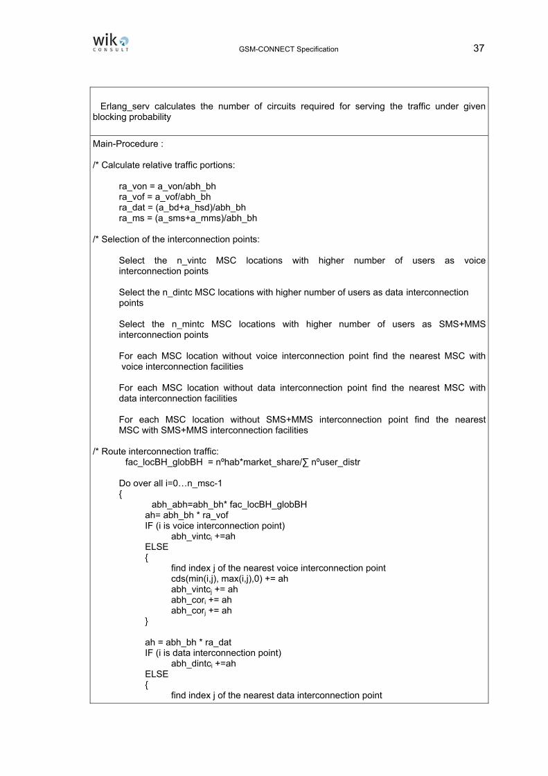
GSM-CONNECT Specification 37
Erlang_serv calculates the number of circuits required for serving the traffic under given blocking probability
Main-Procedure : /* Calculate relative traffic portions: ra_von = a_von/abh_bh ra_vof = a_vof/abh_bh ra_dat = (a_bd+a_hsd)/abh_bh ra_ms = (a_sms+a_mms)/abh_bh /* Selection of the interconnection points: Select the n_vintc MSC locations with higher number of users as voice interconnection points Select the n_dintc MSC locations with higher number of users as data interconnection points Select the n_mintc MSC locations with higher number of users as SMS+MMS interconnection points For each MSC location without voice interconnection point find the nearest MSC with voice interconnection facilities For each MSC location without data interconnection point find the nearest MSC with data interconnection facilities For each MSC location without SMS+MMS interconnection point find the nearest MSC with SMS+MMS interconnection facilities /* Route interconnection traffic:
fac_locBH_globBH = nºhab*market_share/∑ nºuser_distr Do over all i=0…n_msc-1 { abh_abh=abh_bh* fac_locBH_globBH ah= abh_bh * ra_vof IF (i is voice interconnection point) abh_vintci +=ah ELSE { find index j of the nearest voice interconnection point cds(min(i,j), max(i,j),0) += ah abh_vintcj += ah abh_cori += ah abh_corj += ah } ah = abh_bh * ra_dat IF (i is data interconnection point) abh_dintci +=ah ELSE { find index j of the nearest data interconnection point

38 GSM-CONNECT Specification
cds(min(i,j), max(i,j),0) += ah abh_dintcj += ah abh_cori += ah abh_corj += ah } ah = abh_bh * ra_ms IF (i is message interconnection point) abh_mintci +=ah/4 ELSE { find index j of the nearest message interconnection point cds(min(i,j), max(i,j),0) += ah abh_mintcj += ah abh_cori += ah/4 abh_corj += ah/4 } } /* Route voice On-Net traffic Do over all i=0…n_msc-1 rweighi = nmsc_useri / totn_user Do over all i=0…n_msc-1 { ah=ra_von * abh_bh Do over all j=0…n_msc-1 { IF(i ≠j ) { aij =ah * rweighi cds(min(i,j), max(i,j),0) += aij abh_cori += aij abh_corj += aij } } } /* Calculate number of circuits and DSGs for interconnection Do over all i=0…n_msc-1 { IF (abh_vintci > 0) { ncirc= erlang_serv(abh_vintci, block_vintc) nvintc_dsl = ⎡ncirc / maxcdsg⎤ } IF (abh_dintci > 0) { ncirc= erlang_serv(abh_dintci, block_dintc) ndintc_dsl = ⎡ncirc / maxcdsg⎤ } IF (abh_mintci > 0) { nmintc_dsl = ah_mintc/(maxdsg * rho_mint)

GSM-CONNECT Specification 39
} } /* Calculate the required DSG groups on the core links Do over all i=0…n_msc-2 { Do over all i=0…n_msc-1 { ah= cds(i,j,0) IF (ah>0) { ncirc =erlang_serv(ah, block_core) cds(i,j,1) =ncirc cds(i,j,2) = ⎡ncirc / maxcdsg⎤ } } }
The implementation of the physical CORE-DESIGN algorithm is assumed to be similar to the backhaul network, either in the form of DSGs at the STM-1 level leased from another operator or in the form of the operator’s own physical infrastructure. Again as in the case of the backhaul network the WIK-MNCM assumes that a mobile operator implements the physical network using leased lines. The reason is that in case of a stand-alone mobile operator the implementation of an own physical infrastructure is not justified economically and in case that the operator operates both a fixed network and a mobile network the mobile part of the integrated operator’s business will lease these lines from its fixed-line business. This point is considered in further detail in Annex II.
3.6 Parameter values for various scenarios
Previous sections illustrate that the network design requires the adoption of parameter values which are country-specific and service-specific. This section shows how parameter values necessary for network design have been selected. This is done for scenarios that reflect different states of the hypothetical operator in Australia. Regarding the selection of parameter values for the design of the aggregation, backhaul and core networks, sensitivity analyses have been carried out the results of which are shown to lead to optimal values of these parameters. It should be noted that the following sensitivity analyses relate to those of the model implementation as of January 2007.
The objective of the module presented in section 3.1 is the generation of the Districts required for the cell deployment of a network. The starting point is the POA data set, containing information about the number of residents, employees and travellers, geographic coordinates etc. This data is modified as outlined for working population and transient population movements in the POA during working hours and converts POAs

40 GSM-CONNECT Specification
into relevant Districts for network dimensioning using a separate aggregation and exclusion procedure.
The population criteria for the exclusion procedure is reflected for each market share scenario using the following values:
Market share [%] 17 25 31 44
Exclusion threshold [inhabitant] 8500 3500 3500 3500
Nº of excluded POAs 938 763 763 763
Resulting population coverage [%] 92 96 96 96
Number of Districts 463 638 638 638
The corresponding parameter values for the POA aggregation procedure are the same for the four scenarios and are outlined in the following table:
Minimum Medium Maximum
Inhabitants threshold 100 500 1000
Distance threshold [Km] 20 10 5
The Scen-Generator classifies the POAs in each District into three classifications based on density, consistent with the propagation model used by the SNPT as applied in the WIK-MNCM:
WIK-MNCM Urban Classification
Suburban Classification
Rural Classification
Represents Dense urban areas
Urban and suburban areas
Low density and rural areas
3.6.1 Parameter values for the cell deployment
The parameter values are represented by the following three windows:
• General parameters,
• Voice and data service parameters, and
• Other parameters.

GSM-CONNECT Specification 41
General parameters
The general parameter values are the same for all scenarios. Indoor coverage is assumed to be 100 per cent for urban and suburban Districts and 85 per cent for rural Districts in the WIK-MNCM. For all scenarios a dual band operator is assumed to use 900 and 1,800 MHz frequency spectrum. For urban Districts the number of Pico-Cells as calculated by the WIK-MNCM is increased by 20 per cent to account for additional cells for (limited) propagation in tunnels, shadow areas and public indoor areas.
Voice and data Service parameters
Voice and data service parameters are shown below for a variety of scenarios:
Scenario 17% market
share 92% coverage
96% penetration rate
Scenario 25% market
share 96% coverage
96% penetration rate
Scenario 31% market
share 96% coverage
96% penetration rate
Scenario 44% market
share 96% coverage
96% penetration rate
Traffic (mErl) 8.3 8.3 8.3 8.3
On-Net traffic share 18.8 22.6 24.4 31.96
Off-Net Incoming share 37.6 35.7 34.8 31.02
Off-Net Outgoing share 37.6 35.7 34.8 31.02
HSCSDS share 0.8 0.8 0.8 0.8
GPRS share 3 3 3 3
SMS share 0.1 0.1 0.1 0.1
MMS share 0.1 0.1 0.1 0.1
Basic Data share 2 2 2 2
Other parameters
The parameters in the other windows are independent of the relevant scenario and remain constant over any scenario considered.
3.6.2 Parameter values for the aggregation network configuration
The objective of the aggregation network is to identify the network structure, the flow and the links between the different sites and the BSC. The calculation is based on the results obtained from the cell deployment procedure which provides the list of all Districts and their BTS site numbers. The steps for the network configuration are the:

42 GSM-CONNECT Specification
• Selection of the BSC,
• Assignment of the BTS hubs (and hence of the BTSs) to the BSC,
• Identification of the structure between the BTS hubs and the BSC, and
• Routing the demand and carrying out of link calculations.
The selection of the BSC locations is influenced by the following parameter values:
• Number of BSC locations,
• Minimal geographical distance among the BSCs, and
• Maximum number of BTSs which can be aggregated to a BSC location.
The BSC selection considers an optimal solution with reference to two criteria: cost minimisation and network resilience.19 The cost relationships that need to be factored in are: the increase in the total cost of BSC units, as the number of BSC sites increases, against the reduction in the cost of the links between BSC and BTS-hub sites. The following tables show that for the Australian network any cost advantages arising from an increase in the number of BSC sites are not outweighed by the cost increases associated with additional BSCs. Network resilience increases with more BSC sites as there are lower traffic values in the links of the BSCTREE and the corresponding BSC locations. A detailed analysis has shown that the following parameter values provide an optimal solution:
17% market share
25% market share
31% market share
44% market share
Number of BSC locations 20 20 20 30
Minimum distance [Km] 80 80 80 80
Maximum number of BTS locations per BSC 200 200 200 200
The method used for selecting the optimal values is shown for a 25 per cent market share scenario. In the example, the number of BTS locations increases from 15 to 30 in lots of 5 resulting in values for the BTS selection and BTS hub assignment as follows:
19 Network resilience in the context of the WIK-MNCM means the performance of the network topology and its traffic on the network nodes and links against possible failures; e.g. the failure probability of a link increases with the link length and the damage in case of a failure increases with the corresponding traffic flow.

GSM-CONNECT Specification 43
Number of
BSCs Users/BSC
(in thousand) Remote
BTS locations/BSC
Remote BTS hub
locations/BSC
Star link distance
BTS hub-BSC (Km)
Cost/minute for Off-Net
incoming calls (in per cent,
highest value = 100 per cent)
15 380 166.9 41.5 550.9 91.2
20 285 125.2 30.9 189.6 93.8
25 228 100.2 24.5 167.4 97.4
30 190 83.5 20.3 158.3 100.0
A calculation of relative values for the increase in the total cost and the network configuration performance values results in the diagram as shown in Figure 3-7. This figure shows a decrease in the distances between the BTS hubs and the BSC locations because of the increase in the number of BSC locations from 15 to 20 or 66. 6 per cent, while the corresponding cost increase is relatively low (at 2.6 per cent). The cost increase is relatively low as the cost increase due to the increase in the number of BSCs is almost outweighed by the lower costs of shorter distances in the links of the BSC tree which connects the BTS hub locations with the BSC locations. In this way, 20 is determined as the optimal value for the number of BSC locations taking into account both the cost minimisation criterion and the network resilience criterion.
Figure 3-7 Values of resilience and cost parameters as a function of the number of BSCs
0,0
0,2
0,4
0,6
0,8
1,0
1,2
15 20 25 30
Number of BSC
Dep
ende
nt v
aria
ble
(hig
hest
val
ue =
1)
Users/BSCs
BTSs/BSCs
Distance BTSs/BSCs
Distance BTS hubs/BSCs
Cost/minute
Colour Code: Dark blue user/BSC-location; Red nº of remote BTS/BSC-location, Yellow nº of remote Districts/BSC-location, Light blue distance of the star link BTS hub – BSC-location, Pink cost/min for Off-Net incoming voice traffic

44 GSM-CONNECT Specification
The distance between the BSCs is shown to have a small influence on the cost, but has strong implications for network resilience. If a minimum distance restriction is imposed, the BSC layout for the network will be concentrated on the Eastern Seaboard of Australia. However, at least one BSC should be located in Western Australia to reduce the star distance between the BTS hubs and the BSC-locations on the Western-side of Australia. The next table shows these details and why a distance threshold of 80 Km provides an optimal solution.
Distance between BSC locations (Km)
Star link distance BTS hub-BSC (Km)
Cost/minute for Off-Net incoming calls
(in per cent, highest value = 100 per cent)
25 576.5 93.2
50 519.1 96.2
75 508.4 95.8
80 189.7 97.7
100 184.1 100.0
The resulting BSCTREE topology is influenced by a penalty value. The variation of this parameter produces a tree network structure which lies between a pure star topology and the MST. This parameter is set to one in all the scenarios. A detailed analysis of the penalty factor shows that variation in its value does not influence the cost but provides strong variation in the flow on the links, the number of hops for the path from the BTS hubs to the BSC location, and the length of the tree. While the flow and the number of hops are minimised in case of a star topology, the tree length is minimised in a MST. The following table shows the topological characteristics of different penalty values.
Penalty value 0 0.5 1 5 10 50 100 500
Average nº hops 7.57 3.07 2.31 1.26 1.1 1.01 1 1
Average tree length 1581 3276 3778 5046 5421 5706 5732 5860
Average flow on link 199.9 96.7 74.9 39.5 33.7 30 29.7 29.6
Cost/minute 5.851 5.85 5.85 5.85 5.85 5.85 5.85 5.85

GSM-CONNECT Specification 45
The relative increase/decrease of the penalty parameter is illustrated below:
Figure 3-8 Values of characteristic parameters for the BSCTREE as a function of the penalty value
0
0,2
0,4
0,6
0,8
1
1,2
0 0,5 1 5 10 50 100 500
Penalty value
Dep
ende
nt v
aria
ble
(hig
hest
val
ue =
1)
No. of hops
Tree lengthFlow
Cost/minute
To find the optimum penalty value, the relative increase for the tree length and the relative decrease for the flow values need to be mapped as a unique parameter determined by the following formula:
f(relative tree length increase, relative flow decrease) = λ*relative tree length increase + (1-λ)*relative flow decrease
A composite parameter determined on the basis of equal weights for both parameters (λ=0,5) results in an optimal penalty value of 1. The same result is obtained when the relative decreases in the number of hops and the relative decreases in the flow are combined, see Figure 3-9.

46 GSM-CONNECT Specification
Figure 3-9 Values of composite parameters (length and hops; length and flow) as a function of the penalty value
40%
45%
50%
55%
60%
65%
0 0,5 1 5 10 50 100 500
Penatly value
Rel
ativ
e ch
ange
in c
ompo
site
par
amet
er
(%) Length and hops
Length and Flow
3.6.3 Parameter values for the backhaul and core network configuration
The objective of the backhaul network is to connect the BSCs with the MSCs where the WIK-MNCM considers a a star link topology implemented in form of DiLeLs. As already indicated in section 3.4, this topology provides an acceptable network resilience outcome because the operator which provides the leased lines implements the corresponding DSG groups either in a self-healing ring structure based on SDH-ADM equipment or, alternatively, the operator can provide the leased lines in the form of a meshed structure based on digital cross connector equipment which provides a restoration of STM-1 groups in case of failures. The main parameters which influence the network configuration are the number of MSC sites, the maximum number of users which can be connected to that MSC site and the minimum distance between each MSC site. For the different scenarios the following optimal values were used for the relevant parameters.
17% market share
25% market share
31% market share
44% market share
Nº MSC locations 5 5 5 6
Minimum distance (Km) 300 300 300 300
Maximum number of users per MSC location (in thousand) 2000 2000 2000 2000

GSM-CONNECT Specification 47
The main parameters for optimising the cost and network resilience outcomes are the cost per minute of off-net incoming calls and the average number of users connected to an MSC location. With reference to the 25 per cent market share case the number of MSC locations was increased from four to ten. The values are shown in the table below:
Number of MSCs Average number of users/MSC (in thousand)
Cost/minute for Off-Net incoming calls
(in per cent, highest value = 100 per cent)
4 1426 81.7 5 1141 82.3 6 951 85.2 7 815 88.9 8 713 92.5 9 634 96.3 10 571 100.0
The intersection point of the cost per minute of off-net incoming calls and the number of users as a function of the number of MSC sites is shown in Figure 3-10 from which the optimal value of five MSC sites for the 25 per cent scenario can be derived.
Figure 3-10 Cost per minute and average traffic load (expressed by the number of users) as a function of the number of MSC sites
0,3000
0,4000
0,5000
0,6000
0,7000
0,8000
0,9000
1,0000
1,1000
4 5 6 7 8 9 10
Number of MSCs
Dep
ende
nt v
aria
ble
(hig
hest
val
ue =
1)
Users/MSC
Cost/minute

48 GSM-CONNECT Specification
With reference to the minimal distance between the MSC sites, a value of 300 kilometres results in an even distribution of the nodes among the BSC sites with the highest traffic loads, see Figure 3-11.
Figure 3-11 Core network topology for the 25 per cent scenario
For the core network, the WIK-MNCM considers a fully meshed network implemented by DiLeLs based on DSGs at the level of STM-1. The number of core links increases using the equation M = N*(N-1)/2 where M is equal to the number of core links and N is equal to the number of MSC locations. Hence the flow in E1 groups decreases with the lower use of the STM-1. This explains the resulting cost increases shown in Figure 3-10.
Number of MSCs
Total core length (Km)
Average E1 core link flow
Number of STM-1 Groupsper core link
Cost/minute for Off-Netincoming calls
(in per cent, highest value = 100 per
cent) 4 12,468 119 2-1 81.7 5 18,030 75.7 2-1 82.3 6 29,415 52 1 85.2 7 39,102 38 1 88.9 8 48,832 29 1 92.5 9 60,372 23 1 96.3
10 67,365 19 1 100.0

GSM-CONNECT Specification 49
The remaining parameters for the core network configuration are related to the number of interconnection points for the different types of services. As the number of MSCs is small, the WIK-MNCM assumes that each MSC site has interconnection points to other voice networks (PSTN/ISDN or mobile networks); the interconnection point for SMSs is provided at one central point where the required number of SMS service centres are installed.20
20 The number of SMS service centres depends on the SMS service centre capacity and aspects of availability; its corresponding dimensioning is provided by the cost module.

50 GSM-CONNECT Specification
4 Data file specification
The SNPT (is implemented in the form of small independent program modules. These modules need to be run in the following order: data aggregation, cell deployment, aggregation–backhaul and core network design.
4.1 Cell deployment input data files specification
I. Scen File
This is the file path to the rest of the files for each scenario.
<filename>.fic
Name Type Comment
Scen_Name String Name of the scenario
CitiesFP String Path of the cities file
BTSFP String Path of the BTS file
GPFP String Path of the general parameters of the scenario
SPFP String Path of the service parameters file
MPFP String Path of the file with the mobile station parameters

GSM-CONNECT Specification 51
II. District File
This file contains the parameter values for each District considered in the current scenario. The file is named ‘cities’ which is used as a synonym for District.
<scenario_name>_cities.txt
Name Type Comment First Line n_cities Integer Number of cities For each District First Line District_name String Name of the District Second Line n_districtid Int District identifier n_hab Int Number of inhabitants of the District (≥ 0) n_ext_type Bool 0: Radial; 1: Extensión fl_ext Float Radius in Km / extension in Km2 of the District (≥ 0) fl_dutper Float Percentage of urban terrain fl_sutper Float Percentage of suburban terrain fl_restper Float Percentage of rural terrain fl_dupper Float Percentage of urban population fl_supper Float Percentage of suburban population fl_respper Float Percentage of rural population fl_flattper Float Percentage of the District in a flat terrain fl_hilltper Float Percentage of the District in a hilly terrain fl_montper Float Percentage of the District in a mountainous terrain n_bheighth Int Average building height in a high building concentration zone (m) n_bheightl Int Average building height in a low building concentration zone (m)
n_btsheighth Int BTS height in a high building concentration zone (m) (n_bheighth + n_btsheighth > 0)
n_btsheightl Int BTS height in a low building concentration zone (m) (n_bheightl + n_btsheightl > 0)
n_districtproptype Int Type of District for radio propagation studies: 0 Large-Metropolitan, 1- Medium, 2 Small-Rural
fl_tLoss Float Terrain Loss by Orography. Range = (-1000, +1000) [dB] n_intcelltech Int Type of Celullar Technology: 0 TDMA, 1 CDMA 2 WCDMA fl_x Float X Coordinate in UTM or Degrees fl_y Float Y Coordinate in UTM or Degrees

52 GSM-CONNECT Specification
III. BTS File.
This file contains the parameters for each BTS type defined for the current scenario.
<scenario_name>_BTS.txt
Name Type Comment
First Line
n_models Int Number of BTS models
For Each BTS
Sz_name String Name of the model of the BTS
n_radioch Int Number of radio channels. (n_radioch- n_handover- n_signalling > 0)
n_handover Int Number of handover channels
n_signalling Int Number of signalling channels
fl_btsurbpower_tx Double Transmission power in urban zone (>0) [W]
fl_btssurbpower_tx Double Transmission power in suburban zone (>0) [W]
fl_btsrespower_tx Double Transmission power in rural zone (>0) [W]
fl _btsFnoise_rx Double BTS noise figure. Range = (-1000, +1000) [dB]
fl _Losscables Double Cable losses. Range = (-1000, +1000) [dB]
fl _Losscomb Double Losses in the combiners. Range = (-1000, +1000) [dB]
fl _acoupler Double Losses in couplers. Range = (-1000, +1000) [dB]
fl _bts_gain_pre Double Pre-amplifier gain. Range = (-1000, +1000) [dB]
fl _bts_gain_rx Double Transmitter antenna gain. Range = (-1000, +1000) [dB]
fl _bts_gain_tx Double Receiver antenna gain. Range = (-1000, +1000) [dB]
fl _bts_cost Double Cost of the BTS
n_max_sect Int Maximum number of sectors. (>0)
n_min_sect Int Minimum number of sectors. (>0). (n_max_sect - n_min_sect ≥ 0)
n_trxurb Int Number of TRXs per sector in urban zone. (>0)
n_trxsurb Int Number of TRXs per sector in suburban zone. (>0)
n_trxres Int Number of TRXs per sector in rural zone. (>0)
b_av_urb Bool BTS type available in urban zone. (0:No, 1:Yes)
b_av_surb Bool BTS type available in suburban zone. (0:No, 1:Yes)
b_av_res Bool BTS type available in rural zone. (0:No, 1:Yes)
b_av_dualb Bool BTS type available for Dual Band. (0:No, 1:Yes)

GSM-CONNECT Specification 53
IV. General File
This is a miscellaneous file containing the general configuration of the current scenario.
<scenario_name>_general.txt
Name Type Comment
fl_1bulf Double 1st band uplink frequency. (>0) [MHz]
fl_1bdlf Double 1st band downlink frequency. (>0). [MHz]. fl_1bulf & fl_1bdlf must be in the same band
b_2b Bool 0: One band ; 1: Dual band
fl_2bulf * Double 2nd band uplink frequency. (>0). [MHz]
fl_2bdlf * Double 2nd band downlink frequency. (>0). [MHz]. fl_2bulf & fl_2bdlf must be in the same band
fl_ffm Double Fast fading margin. Range = (-1000, +1000) [dB]
fl_lnm Double Log. Normal fading Margin. Range = (-1000, +1000) [dB]
fl_Im Double Interference Margin. Range = (-1000, +1000) [dB]
Fl_build_loss Double Building penetration loss. Range = (-1000, +1000) [dB]
Fl_sub_reduction Double Building loss suburban reduction factor. (0-1)
Fl_rural_reduction Double Building loss rural reduction factor. (0-1)
N_sectoriz_method Bool Sectoriz. Method: 0: aggreg. 1: sharing equipment
N_reserved Int Reserved for future use
N_dont_sectorize Bool 0: Sectorise; 1: Don’t sectorie
N_sector_cost Int Sectoring cost factor. (0-1)
n_anatype Int Type of analysis: 0: First minimise cost, Second minimise # BTSs; 1: First minimise # BTSs, Second minimise cost.
fl_Test1 Double Relative urban coverage value. Not applicable to a network in Australia. Not used in version 1.1 of the WIK MNCM.
fl_Test2 Double Relative suburban coverage. Not applicable to a network in Australia. Not used in version 1.1 of the WIK MNCM
fl_Test3 Double Relative rural coverage value. Not applicable to a network in Australia. Not used in version 1.1 of the WIK MNCM
fl_minimum_density Double Minimum population density evaluative
N_zone_type Bool 0: block zones; 1: annular zones
* : Only present if b_2b is equal to ‘1’
V. Service File
This file describes the parameters of each service considered in the WIK-MNCM.
<scenario_name>_services.txt.

54 GSM-CONNECT Specification
Name Type Comment
fl_voice_lambda_on Double Call origination and termination rate in the BH for On-Netvoice service [calls in BH] (≥ 0)
fl_voice _ts_on Double Service time for On-Net voice service [sec] (≥ 0)
fl_voice_lambda_off Double Call origination and termination rate in the BH for Off-Netvoice service [calls in BH] (≥ 0)
fl_voice _ts_off Double Service time for Off-Net voice service [sec] (≥ 0)
n_gprs_ns Integer Average number of slots used in GPRS connection (≥ 0)
fl_gprs_lp Double GPRS data packet length [bytes] (≥ 0)
fl_gprs_np Double Average number of packets transmitted in GPRS connection (≥ 0)
fl_gprs_lambda Double GPRS connection rate in the BH [connections / hour] (≥ 0)
fl_gprs_ts Double Service time for GPRS connection in the BH [s] (≥ 0)
n_hscsd_ns Integer Average number of slots used in HSCSDS connection (≥ 0)
fl_hscsd_lambda Double HSCSDS connection rate in the BH [connections / hour] (≥ 0)
fl_hscsd_ts Double Service time for HSCSDS [s] (≥ 0)
fl_data_lambda Double Basic data connection rate (MODEM) [connections/hour] (≥ 0)
fl_data_ts Double Basic data service time (MODEM) [s] (≥ 0)
n_sms_length Integer SMS message length. [bytes] (≥ 0)
fl_sms_lamda Double SMS sending rate [sms/hour] (≥ 0)
n_mms_ns Integer Average number of slots used in GPRS/MMS connection (≥ 0)
n_mms_length Integer MMS message length [bytes] (≥ 0)
fl_mms_lamda Double MMS sending rate [MMS/hour] (≥ 0)
fl_avumov Double Average user movement speed [Km/h] (≥ 0)
fl_ms Double Operator market share (0-1)
fl_mp Double Mobile market penetration in the country (0-1)
fl_blockprob Double Service blocking probability (0-1)

GSM-CONNECT Specification 55
VI. Mobile Station File
This file describes the characteristics of the mobile station.
<scenario_name>_mobile.txt.
Name Type Comment
Fl_tx_power Double Mobile transmission power [W] (>0)
Fl_mobile_height Double Mobile average height [metres] (>0)
Fl_rx_noise Double Mobile receiving noise figure. Range = (-1000, +1000) [dB]
Fl_gain Double Mobile gain. Range = (-1000, +1000) [dB]
Fl_skin_loss Double Mobile skin loss. Range = (-1000, +1000) [dB]
Fl_mismatch Double Mobile mismatch. Range = (-1000, +1000) [dB]
4.1.1 Output files
I. BTS deployment (abstract).
<scenario_name>_outputBA.txt
Name Type Comment
int_districtid Integer Identifier of the District
sz_districtname String Name of the District
sz_BTSurb String Type of BTSs in urban zone
sz_BTSsub String Type of BTSs in suburban zone
sz_BTSres String Type of BTSs in rural zone
n_TRXnumber Integer Total number of TRXs
n_TRXurb Integer Number of TRXs in urban
n_TRXsub Integer Number of TRXs in suburban
n_TRXres Integer Number of TRXs in rural
n_BTSTotal Integer Total Number of BTSs
n_BTSurb Integer Number of BTSs in urban zone
n_BTSsub Integer Number of BTSs in suburban zone
n_BTSres Integer Number of BTSs in rural zone
fl_TrafficTotal Float total traffic in the District
fl_Trafficurb Float Traffic in urban zone
fl_Trafficsub Float Traffic in suburban zone
fl_Trafficres Float Traffic in rural zone
fl_X Float X coordinate in UTM or degrees
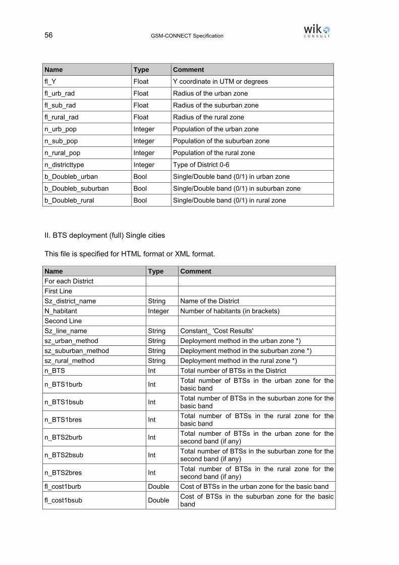
56 GSM-CONNECT Specification
Name Type Comment
fl_Y Float Y coordinate in UTM or degrees
fl_urb_rad Float Radius of the urban zone
fl_sub_rad Float Radius of the suburban zone
fl_rural_rad Float Radius of the rural zone
n_urb_pop Integer Population of the urban zone
n_sub_pop Integer Population of the suburban zone
n_rural_pop Integer Population of the rural zone
n_districttype Integer Type of District 0-6
b_Doubleb_urban Bool Single/Double band (0/1) in urban zone
b_Doubleb_suburban Bool Single/Double band (0/1) in suburban zone
b_Doubleb_rural Bool Single/Double band (0/1) in rural zone
II. BTS deployment (full) Single cities
This file is specified for HTML format or XML format.
Name Type Comment For each District First Line Sz_district_name String Name of the District N_habitant Integer Number of habitants (in brackets) Second Line Sz_line_name String Constant_ 'Cost Results' sz_urban_method String Deployment method in the urban zone *) sz_suburban_method String Deployment method in the suburban zone *) sz_rural_method String Deployment method in the rural zone *) n_BTS Int Total number of BTSs in the District
n_BTS1burb Int Total number of BTSs in the urban zone for the basic band
n_BTS1bsub Int Total number of BTSs in the suburban zone for the basic band
n_BTS1bres Int Total number of BTSs in the rural zone for the basic band
n_BTS2burb Int Total number of BTSs in the urban zone for the second band (if any)
n_BTS2bsub Int Total number of BTSs in the suburban zone for the second band (if any)
n_BTS2bres Int Total number of BTSs in the rural zone for the second band (if any)
fl_cost1burb Double Cost of BTSs in the urban zone for the basic band
fl_cost1bsub Double Cost of BTSs in the suburban zone for the basic band

GSM-CONNECT Specification 57
Name Type Comment fl_cost1bres Double Cost of BTSs in the rural zone for the basic band
fl_cost2burb Double Cost of BTSs in the urban zone for the second band (if any)
fl_cost2bsub Double Cost of BTSs in the suburban zone for the second band (if any)
fl_cost2bres Double Cost of BTSs in the rural zone for the second band (if any)
Fl_total_cost Double Total cost of the deployment Third, Fourth, Fifth Lines Optional depending on existing traffic on each zoneFor each zone Sz_zone_name String Zone name Sz_bts_model String Name of the BTS model Fl_tx_power Double BTS Nominal transmission Power N_sector Integer # sectors N_bands Bool Single/Double Band (0/1) Fl_cell_radius Double Cell radius Fl_traffic Double Traffic N_reduction Bool Enable/Disable reduction (0/1) Fl_red_perc Double Reduction percentage Fl_new_tx_power Double New transmission power N_rchannel Integer # Radio channel N_hchannel Integer # Handover channel N_schannel Integer # Signalling channel Fl_cable_loss Double Cable loss Fl_comb_loss Double Combinator loss Fl_coupler_loss Double Multicoupler loss Fl_rx_noise Double BTS receiver noise Fl_rx_gain Double BTS receiver gain Fl_tx_gain Double BTS transmission gain Fl_pre_gain Double BTS pre gain fl_bts_cost Double BTS cost Sixth, Seventh, Eighth Lines Optional depending on existing second band For each zone on second band Sz_zone_name String Zone name Sz_bts_model string Name of the BTS model Fl_tx_power Double BTS nominal transmission power N_sector Integer # sectors Fl_1br_2br_ratio Double First band BTS radius per second Band BTS radiusFl_cell_radius Double Cell radius Fl_traffic Double Traffic N_reduction Bool Enable/Disable reduction (0/1) Fl_red_perc Double Reduction percentage Fl_new_tx_power Double New transmission power N_rchannel Integer # Radio channel N_hchannel Integer # Handover channel

58 GSM-CONNECT Specification
Name Type Comment N_schannel Integer # Signalling channel Fl_cable_loss Double Cable loss Fl_comb_loss Double Combinator loss Fl_coupler_loss Double Multicoupler loss Fl_rx_noise Double BTS receiver noise Fl_rx_gain Double BTS receiver gain Fl_tx_gain Double BTS transmission gain Fl_pre_gain Double BTS pre gain fl_bts_cost Double BTS cost
*) The deployment method may be:
1. BTSs without sectorisation, 2. BTSs sectorisation, 3. Cell radius reduction, 4. Two frequency bands.
III. Service_equivalent_traffic file
<scenario_name>_indvsratio.txt
Name Type Comment
First Line
fl_ratevoice_on Double Percentage per user of On-Net voice traffic
fl_ratevoice_off_in Double Percentage per user of incoming Off-Net voice traffic
fl_ratevoice_off_out Double Percentage per user of outgoing Off-Net voice traffic
fl_rategprs Double Percentage per user of GPRS traffic
fl_ratehscsd Double Percentage per user of HSCSDS traffic
fl_ratemodem Double Percentage per user of MODEM traffic
fl_ratesms Double Percentage per user of SMS traffic
fl_ratemms Double Percentage per user of MMS traffic
Second Line
fl_adivrate_on Double Equivalent service time for voice On-Net
fl_ adivrate _off_in Double Equivalent service time for voice Incoming Off-Net
fl_ adivrate _off_out Double Equivalent service time for voice outgoing Off-Net
fl_ adivrate gprs Double Equivalent service time for GPRS
fl_ adivrate hscsd Double Equivalent service time for HSCSDS
fl_ adivrate modem Double Equivalent service time for MODEM

GSM-CONNECT Specification 59
Name Type Comment
fl_ adivrate ms Double Equivalent service time for SMS
fl_ adivrate mms Double Equivalent service time for MMS
Third Line Double
fl_locbhglobhratio Double Local BH to global BH ratio.
4.1.2 File for the evaluation of the results
I. BTS deployment (Summarise).
<scenario_name>_outputSBH.txt
Name Type Comment
First Line
n_totalpop Int Total population
n_totalcovpop Int Covered population
fl_popcovperc Double Percentage of covered population
n_modtotpop Int Total modified population
fl_mp Double Market penetration
fl_ms Double Market share
fl_locbhglobbhratio Double Ratio global BH to local BH
BTS Type Total nº sites Total nº of BTS
1
2
3
…
Total
4.2 Aggregation network data file specification
As shown in section 3.2, the deployment of the aggregation network is composed of three algorithms which are implemented in the form of three functions, each of which is implemented in form of a ‘Dynamic Link Library’ (DLL) where the three DLLs use a

60 GSM-CONNECT Specification
common data structure. The first function reads from the output files of the cell deployment procedures, as outlined in section Error! Reference source not found., and calculates the values of the corresponding variables; then this output is used by the next function for loading the input data for the common data structure. This step is repeated by the third function which generates the external output files required for the deployment of the backhaul network dimensioning.
Each function generates output data files and another file which provides the results from an evaluation of the solution. This information provides detailed information about the numerical behaviour of the algorithm under a set of parameter values and therefore the study of the influence of the parameter values on the network configuration can be examined. The report titled ‘Mobile Termination Cost Model for Australia, January 2007’ (the Report) shows results for the most important parameters and derives from these the optimal parameter values
I. BTS deployment, refer to section 4.1.2 (I) for details
II. Parameters file:
Value Type Comments n_bsc Integer Number of BSC locations btsmax Integer Maximum number of BTSs assignable to a BSC btsmin Integer Minimum number of BTSs assignable to a BSC epsilon Real Distance increment factor for re-assignation dmin Real Minimum distance between BSCs nlbscmax Integer Maximum number of radio links connected to a BSC
nlbtsmax Integer Maximum number of radio links connected to a BTS District (excluding internal radio links)
lmax Real Maximum length of the radio link
4.2.1 Output files
The aggregation network procedure generates two output files, one containing the resulting BSC locations and their characteristic values and one containing the links of the external trees connecting the BTS locations to the corresponding BSCs.
I. BSC_list
<scenario_name>_an_bsc.txt
Value Type Comments name Character BTS District name of the BSC location

GSM-CONNECT Specification 61
Value Type Comments code Integer BTS District code x_coor Real Horizontal coordinate y_coor Real Vertical coordinate totbtsz_bcc Integer Number of BTS Districts aggregated to the BSC location totbts_bsc Integer Number of aggregated BTSs to the BSC location tottrx_bsc Integer Number of aggregated TRXs totAbh_bsc Real BH traffic in Erlang aggregated at the BSC location totnus_bsc Integer Number of users aggregated at the BSC location ne1 Integer Number of E1 DSGs from the BTS hub co-located with the BSC totce1 Integer Total number of E1 DSGs aggregated from the BTS hubs assigned
II. Link_chain_output
<scenario_name>_an_link.txt
Name Type Comments
name Character District name
code Integer District code
nbts Integer Number of aggregated BTSs in the District
ntrx Integer Number of aggregated TRXs in the District
abh Real Aggregated BH traffic in Erlang in the District
x_coor Real Horizontal coordinate
y_coor Real Vertical coordinate
ngrad Integer Number of links connecting at the District
distbsc Real Star distance from the BTS District to its BSC; zero in case of BSC node
pre Integer Code upstairs BTS District of the link; zero in the case of BTS in the BSC location
length Real Length of the link outgoing from BTS in direction to the BSC
lfr Integer Flow of TRXs aggregated at the link outgoing from the BTS
la Real Traffic flow (in BH Erlang) aggregated at the link outgoing from the BTS
nrhop Integer Number of hops from BTS to the BSC; zero in case of BTS in the BSC location
distchain Real Total length over the links from the BTS to the BSC; zero in the BSC location
ncirc Integer Number of 64 Kbps channels
ne1 Integer Number of E1 DSGs
III. Nodes general information (full)
<scenario_name>_an_nod.txt
Name Type Comments

62 GSM-CONNECT Specification
Name Type Comments
name Character District name
code Integer District code
nbts Integer Number of BTSs in the District
ntrx Integer Number of TRXs in the District
abh Real BH traffic in Erlang in the District
x_coor Real Horizontal coordinate of the central point of the District
y_coor Real Vertical coordinate of the central point of the District
ptpral Integer Indicator whether FWC can by applied (0) or PTPRAL must be applied (1)21
level Integer level of the node/ 1: BSC ; 0: pure District
bscasig Integer Pointer to the corresponding BSC location the BTS_district is assigned
nbtsdis Integer number of BTS Districts assigned to a BSC; zero in case of a pure BTS_district
totcbts Integer Total number of BTSs in the BSC Cluster; zero in case of a pure BTS_district
totcuser Integer Total number of users in the BSC Cluster; zero in case of a pure BTS_district
totctrx Integer Total number of TRXs in the BSC Cluster; zero in case of a pure BTS_district
totcabh Real Total traffic in BH Erlang in the BSC Cluster; zero in case of a pure BTS_district
distbsc Real Distance from the BTS District to its BSC; zero in case of BSC node
pre Integer Pointer to the next BTS_district of the chain to the BSC_location, zero in the case of BTS in the BSC location
nrhop Integer Number of hops from BTS to the BSC, zero in case of BTS in the BSC location
dist_up Real Length of the link between a BTS and the next one in the path to the assigned BSC
ngrad Integer Number of links
distchain Real Link length from the BTS to the assigned BSC
lfr Integer Flow of TRXs aggregated at the link outgoing from the BTS
la Real Traffic flow (in BH Erlang) aggregated at the link outgoing from the BTS
mlengthbts Mean length of a BTS link
mtrxbts Mean number of TRXs in a BTS link
mabhbts Mean traffic in the BH in a BTS link
mcircbts Mean number of circuits in a BTS link
ncirc Number of 64 Kbps channels
21 Currently out of use; a complete PTPRAL network is assumed for the aggregation part.
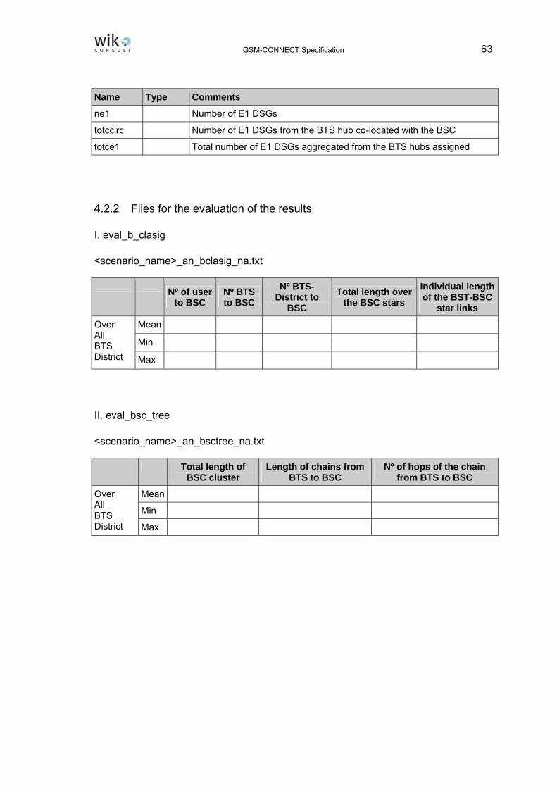
GSM-CONNECT Specification 63
Name Type Comments
ne1 Number of E1 DSGs
totccirc Number of E1 DSGs from the BTS hub co-located with the BSC
totce1 Total number of E1 DSGs aggregated from the BTS hubs assigned
4.2.2 Files for the evaluation of the results
I. eval_b_clasig
<scenario_name>_an_bclasig_na.txt
Nº of user to BSC
Nº BTS to BSC
Nº BTS-District to
BSC Total length over
the BSC stars Individual length of the BST-BSC
star links
Mean Min
Over All BTS District Max
II. eval_bsc_tree
<scenario_name>_an_bsctree_na.txt
Total length of BSC cluster
Length of chains from BTS to BSC
Nº of hops of the chain from BTS to BSC
Mean
Min
Over All BTS District Max

64 GSM-CONNECT Specification
III. eval_ro&ral_asig
<scenario_name>_an_roralasig_na.txt
Nº of TRX aggregated on
BSC
Traffic aggregated
at BSC TRX flow on
links Traffic flow on
links
Mean Min
Over All BTS District Max
4.3 Backhaul network data file specification
As shown in section 3.3, the deployment of the backhaul network comprises one algorithm which again is implemented in the form of a DLL.
In addition to the output data files, the DLL generates a file containing the backhaul network solution. This file provides the user with detailed information about the numerical behaviour of the algorithm when varying sets of parameter values are used. Again the user can examine the set of parameter values after each step in the procedure.
4.3.1 Input files
I. BSC list, refer to section 4.2.2 (I)
II. Parameter file
Value Type Comments
n_msc Integer Number of MSC locations
usermax Integer Maximum number of users assignable to a MSC
usermin Integer Minimum number of users assignable to a MSC
epsilon Real Distance increment factor for re-assignation
dmin Real Minimum distance between MSCs
ploss Real Loss probability
maxcdsg Integer Maximum number of circuits per DSG

GSM-CONNECT Specification 65
4.3.2 Output files
The design and dimensioning step for the backhaul network provides two output files, one containing MSC locations and their characteristic values and one containing the links of the star topology connecting the BSC locations with their corresponding MSCs.
I. MSC_list
<scenario_name>_bn_msc.txt
Value Type Comments
name Character District name of the MSC location
code Integer District code
x_coor Real Horizontal coordinate
y_coor Real Vertical coordinate
totbsc_msc Integer Number of BSCs aggregated to the MSC location
tottdsg_msc Integer Number of aggregated digital signal groups
totabh_msc Real BH traffic in Erlang aggregated to the MSC location
totnus_msc Integer Number of users aggregated to the MSC location
totctrx Integer Number of TRXs aggregated to the MSC location
ndsg Integer Number of E1 DSGs from the BSC co-located with the MSC
II. MSC_Star_list
<scenario_name>_bn_link.txt
Name Type Comments
Namebsc Character BSC name of the BSC location
Codebsc Integer BSC code
codemsc Integer MSC code
length Real Length of the link outgoing from BSC in the direction to the MSC
fdsg Integer Flow of DSGs aggregated at the link
la Real Traffic flow (in BH Erlang) aggregated at the link
totctrx Integer Number of TRXs in the link

66 GSM-CONNECT Specification
III. Backhaul Network – Node Information File
<scenario_name>_bn_nod.txt
Value Type Comments
name Character District name where BSC is installed
code Integer District code
x_coor Real Horizontal coordinate of the BSC location
y_coor Real Vertical coordinate of the BSC location
nuser Integer Number of users connected to a BSC
ndsg Integer Number of DSGs (DS1 or E1) required between the BSC and MSC
abh Real BH traffic in Erlang at the BSC
level Integer level of the node 1: MSC; 0: pure BSC District
mscasig Integer Pointer to the corresponding MSC location to which the BSC is assigned
distmsc Real Distance from the BSC to its MSC; zero in the case of MSC location
nbsc Integer Number of BSC locations assigned to a MSC; zero in case of a pure BSC location
totcuser Integer Total number of users in the MSC Cluster; zero in case of a pure BSC location
totcdsg Integer Total number of DSGs in the MSC Cluster; zero in case of a pure BSC location
totcabh Real Total traffic in BH Erlang in the MSC Cluster; zero in case of a pure BSC location
4.3.3 Files for the evaluation of the results
I. eval_m_clasig
<scenario_name>_bn_mclasig_na.txt
Nº of user to MSC
Nº BSC to MSC
BH traffic
Nº of DSG
Sum of star link length
Mean Min
Over All MSC cluster Max

GSM-CONNECT Specification 67
II eval_backhaul_link
<scenario_name>_bn_links_na.txt
Length DSG flow BH traffic
Mean Min
Over All MSC cluster
Max
4.4 CORE-DESIGN data file specification
4.4.1 Input files
I. MSC_list refer to section 4.3.2 (I)
II. Service equivalent traffic file refer to section 4.1.2 (III)
III. General Parameter file
Name Type Comment n_vintc Integer Number of MSC locations with voice interconnection n_dintc Integer Number of MSC locations with data service interconnection n_mintc Integer Number of MSC location with message service centre block_vintc Real Blocking probability for VoIP on VoIP interconnection facility block_dintc Real Blocking probability for data on data interconnection facility block_core Real Blocking probability on core links rho_mint Real Use degree of the capacity for access to the SMS&MMS server maxcdsg Integer Maximum number of circuits per DSG ringalg Integer Physical layer algorithm identifier. 1: BUS, 3: Ring, 4: MST thr116 Integer Minimum number of STM-1 to constitute an STM-16 maxe1stm1 Integer Maximum number of E1 groups per STM-1 wtrafred Real Traffic reduction for Western Australian locations
4.4.2 Output files
The design and dimensioning step for the core network provides two output files one containing an extended MSC list and the other containing a list of all core links.

68 GSM-CONNECT Specification
I. Extend_MSC_list
<scenario_name>_cn_msc.txt
Value Type Comments name Character District name where MSC is installed code Integer District code x_coor Real Horizontal coordinate of the MSC location y_coor Real Vertical coordinate of the MSC location nmsc_user Integer Number of users connected to the MSC cluster
nbh_dsg Integer Number of DSGs (DS1 o E1) required for BSC-MSC backhaul connections
abh_bh Real BH traffic in Erlang from BSC to MSC backhaul connections asigv Integer Assigned MSC location where voice Off-Net interconnection is provided asigd Integer Assigned MSC location where data traffic interconnection is provided asigm Integer Assigned MSC location where SMS and MMS server are situated vintc Bool Voice Off-Net interconnection facilities installed dintc Bool Data traffic interconnection facilities installed mintc Bool SMS and MMS service centre installed interndsg Integer DSG for internal traffic internabh Real Internal traffic ncoredsg Integer Number of DSGs (DS1 or E1) required for MSC_MSC core connections abh_core Real BH traffic in Erlang from MSC-MSC core connections nvintc_dsg Integer Number of DSGs (DS1 or E1) required for Voice Off-Net interconnection abh_vintc Real BH traffic in Erlang for Voice Off-Net interconnection ndintc_dsg Integer Number of DSGs (DS1 or E1) required for data interconnection abh_dintc Real BH traffic in Erlang for data interconnection
nmintc_dsg Integer Number of DSGs (DS1 or E1) required for interconnection with SMS and MMS servers
abh_mintc Real BH traffic in Erlang for SMS and MMS interconnections nstm1c Integer STM-1 flow to the core network ADM4c Integer Number of ADM4s ADM16c Integer Number of ADM16s AD4c Integer Number of AD-4 cards AD16c Integer Number of AD-16 cards

GSM-CONNECT Specification 69
II. Core_link_list
<scenario_name>_cn_link.txt
Value Type Comments code1 Integer District code code2 Integer District code length Real Length of the core link bhlinktraf Real Aggregated BH traffic with reference to DS0 circuits linkcirc Integer Number of DS0 circuits aggregated on the link linkdsg Integer Number of DSGs required on the link
III. Core physical_link_list
<scenario_name>_phytop.txt
Value Type Comments
code1 Integer District code
code2 Integer District code
length Real Length of the core link
stm4 Real Number of STM-4 systems
stm16 Integer Number of STM-16 systems
FibreKm Integer Fibre kilometres on the link

70 GSM-CONNECT Specification
4.4.3 Files for evaluating the results
I. eval_core_design
<scenario_name>_cn_core_na.txt
Total value per MSC Mean Min Max
BH internal traffic
BH traffic with other MSC
BH traffic with On-Net interconnection facilities
BH traffic with data interconnection facilities
BH traffic with messages servers
DSGs with BSC
DSGs with core links
DSGs with On-Net interconnection facilities
DSGs with data interconnection facilities
DSGs with messages servers
Overall DSGs
II. eval_core_link
<scenario_name>_cn_link_na.txt
Total value per core link Mean Min Max
Length
BH traffic
DS0 circuits
DSGs

GSM-CONNECT Specification 71
Annex I: Consideration of traffic values in the local BH of a District and in the global BH in a MSC due to user mobility
In today’s communication networks there are always two BHs: the morning BH caused by traffic from, to and between business customers and the afternoon BH mainly caused by residential customers. In the legacy PSTN it has usually been assumed that the traffic in the morning BH is dominant.
Global average values over all customers for the two parameters calling rate (α) and average duration (ts) are considered for the dimensioning of the network. This can be considered as the correct approach for the switching equipment because it aggregates a sufficiently high volume of traffic. In this way, the average value over all types of customers is a satisfactory solution. In rural regions it provides for solutions which over-engineer the network due to a lower calling rate and call duration from customers located in these areas. This concept cannot be applied in mobile networks for the following reasons. The BTS dimensioning provides for a limited area of coverage and over-engineering is not acceptable due to the bandwidth limitation in the radio access interface. On the other hand, an under-dimensioning is not acceptable for BTSs in commercial and business (urban) Districts. As a consequence, the number of users in a BTS area is the number of residential users and employees reduced to account for any residential users that are also employees in that area. Hence, a morning peak BH traffic is represented by the total number of users multiplied by the mean traffic value per user, and the afternoon peak traffic by the number of residential users multiplied by the mean traffic value per user.
This leads to the following results for a zone inside a District:
Amorningzone = a * (nºinhabzone + nºemplzone – fzoneempl*nºinhabzone) * markshare
Aaftzone = a * inhabzone * markshare
The dimensioning of network elements higher up in the network hierarchy, like the MSC, has to consider the maximum (traffic) value of the two BHs. In the morning BH the traffic values for residential users is small relative to the working population, this means that a high number of residents are using their mobile handsets for business calls in business zones of a District at this time. As a result, the traffic in the suburban areas in the morning is very low while the traffic in the urban zones is high. In the afternoon BH, the employees return home, so it can be assumed that the afternoon BH is the dominant factor required for the dimensioning of network elements higher up in the network hierarchy, mainly in the MSC, and should closely reflect the number of residents.
The higher local traffic required in the business (urban) zones is already considered by the SNPT by the above formula (Amorningzone). Therefore, no change in the program is

72 GSM-CONNECT Specification
required. The assumption of a dominant afternoon BH is supported by the general tendency in communication networks for strong use by residents.22
For the calculation of the daily traffic the afternoon BH is used as the basis. Hence it is concluded that employees need only be considered for the purpose of local dimensioning in business (urban) Districts.
22 See Khedher (2003), pp. 46-49.

GSM-CONNECT Specification 73
Annex II: Study for the physical layer of a core network
The first solution analysed assumes a cable topology in the form of a bus. Fibre layers also assume a bus, with SDH line terminals installed at both ends (i.e. at each MSC location) and in the intermediate nodes. The figure below shows the topology and the corresponding equipment.
X X X
RegeneratorRegenerator
Perth Adelaide/ Melbourne/ Sydney Brisbane
OC-48 OC-48
STM-1
STM-1
E1
STM-1/OC-48 line terminal
The calculation of the different scenarios for the mobile traffic routed over the links between the five MSCs in the 25 per cent scenario gives an E1 demand which is satisfied by only one STM-1 group. This results in a fully meshed STM-1 structure among all pairs of MSCs. The projection of this demand into a bus topology leads to four STM-1 groups in the two links at the bus terminations on both sites and six STM-1 groups in the two intermediate links. If the transmission is assumed to be implemented by a modern STM-16 (OC-48) optical carrier, only one system is required on each link, and it is used with reference to the occupied STM-1 as 4/16 or 6/16, respectively.
The second solution assumes again a cable topology in the form of a bus connecting the five MSC nodes but implements the bus inside a fibre ring under the SDH self-healing ring concept. The figure below shows this concept schematically.
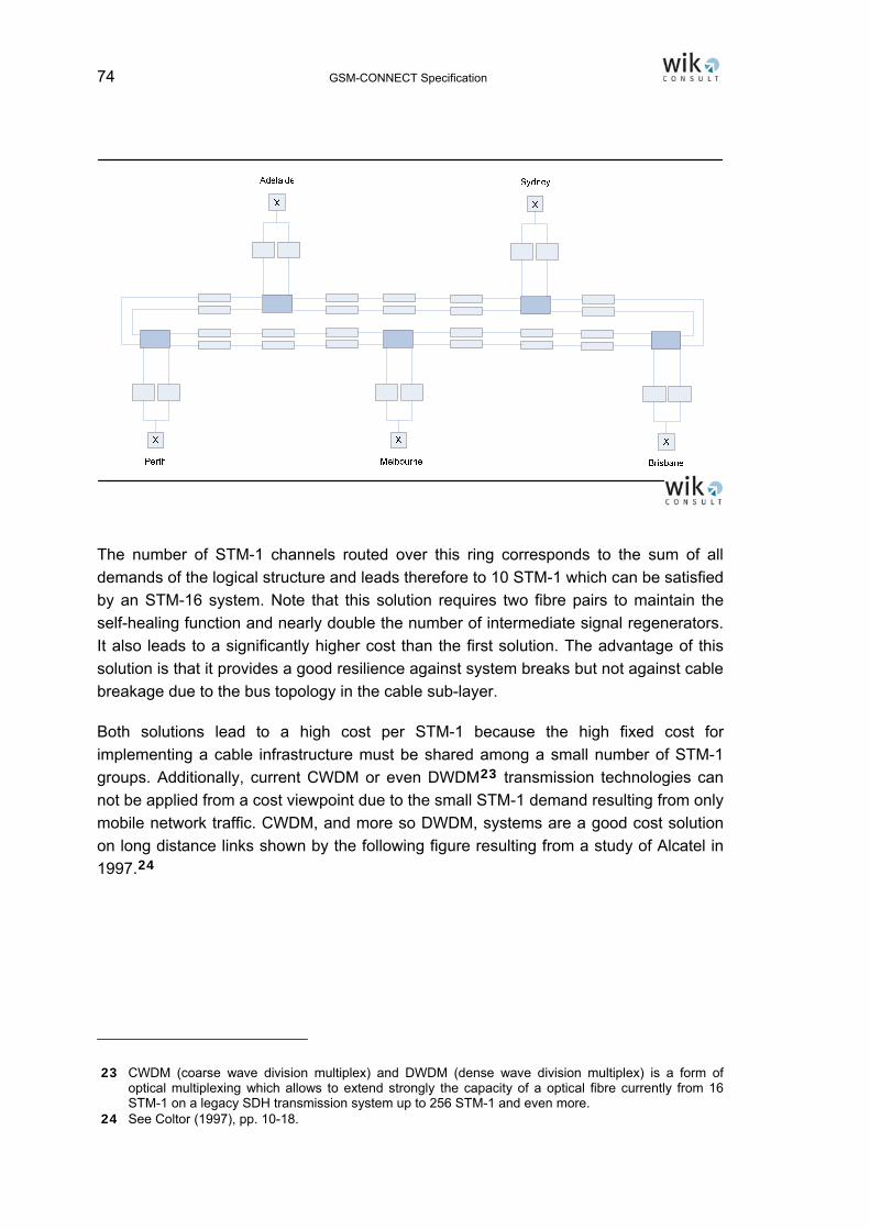
74 GSM-CONNECT Specification
The number of STM-1 channels routed over this ring corresponds to the sum of all demands of the logical structure and leads therefore to 10 STM-1 which can be satisfied by an STM-16 system. Note that this solution requires two fibre pairs to maintain the self-healing function and nearly double the number of intermediate signal regenerators. It also leads to a significantly higher cost than the first solution. The advantage of this solution is that it provides a good resilience against system breaks but not against cable breakage due to the bus topology in the cable sub-layer.
Both solutions lead to a high cost per STM-1 because the high fixed cost for implementing a cable infrastructure must be shared among a small number of STM-1 groups. Additionally, current CWDM or even DWDM23 transmission technologies can not be applied from a cost viewpoint due to the small STM-1 demand resulting from only mobile network traffic. CWDM, and more so DWDM, systems are a good cost solution on long distance links shown by the following figure resulting from a study of Alcatel in 1997.24
23 CWDM (coarse wave division multiplex) and DWDM (dense wave division multiplex) is a form of optical multiplexing which allows to extend strongly the capacity of a optical fibre currently from 16 STM-1 on a legacy SDH transmission system up to 256 STM-1 and even more.
24 See Coltor (1997), pp. 10-18.

GSM-CONNECT Specification 75
In contrast, a fully integrated SDH transport network aggregates a large number of STM-1 channels mainly due to the traffic from broadband services. It allows also the use of modern optical technology inside the transport network and hence provides strong network resilience and the capacity of a restoration of connections inside 50 milliseconds in the case of failures. The next figure shows the main building elements for this integrated electrical optical transport network infrastructure which is composed of electrical cross-connector equipment. The high cost of this equipment is only justified when it is shared across a large bandwidth demand resulting in a fully integrated network platform.
XMux E1/
STM-1
Cross-connector
Optical Mux OC-48/ OC-192 or optical Cross-conn.
Opt. Reg.
1
4
OC-48STM-1E1
1
63
.
.
.
Cable
E1 layerSTM-1 layer
OC-48 layer
Transmission layer OC-192
Regeneration layer


GSM-CONNECT Specification 77
References
Coltor, C. (1997) "Evolution of Transport Network Architecture”, Alcatel Telecommunication Review, 1st Quarter, pp. 10-18
Domschke, W., Drexl, A. (1990) Logistik: Standorte, 3rd Edition, R. Oldenbourg Verlag, München
Flood, J.E. (ed.) (1997) "Telecommunication Networks 2nd Ed.", IEE Telecommunication Series 36, The Institute of Electrical Engineers, London
Gonzalez F., Kulenkampff, G. Hackbarth, K. Rodriguez de Lope, L. (2002) "Network cost models and its application to telecom regulation issues", 13th European Conference of the International Telecommunication Society, Madrid
Hackbarth, K. D., Portilla, J.A., Díaz, C. (2005) "Cost Models for Telecommunication networks and their application to GSM systems", in Paganini, M. (ed.): The Encyclopaedia of Multimedia Technology and Networking, Idea Group Hershey, USA, pp. 143-150
Han, Raj, A. (2003) "GRASP heuristic for solving the extended capacitated concentrator location problem", International Journal of Information Technology & Decision Making, Vol. 2, December, pp. 597-618
Khedher, H., Valois, F., Tabbane, S. (2003) "Channel Holding Time Characterization in real GSM network", 14th IEEE 2003 International Symposium on Personal, Indoor and Mobile Radio Communication Proceedings, pp. 46-49


![SPECIFICATION & INSTALLATION GUIDE52 gsm to 450 gsm (Plain, Fine, Color Specific, Coated-G, Coated-M) 81 gsm to 350 gsm (Textured) 70 gsm to 100 gsm (Envelopes) ... Envelope Seam [1]](https://img.pdfslide.us/doc/110x75/5ebee13946efcd7097328efd/specification-installation-52-gsm-to-450-gsm-plain-fine-color-specific.jpg)


![CS-Tool - SPD[Spreadtrum] Phones Success Reports - GSM-Forum](https://img.pdfslide.us/doc/110x75/577c785f1a28abe0548fcbc4/cs-tool-spdspreadtrum-phones-success-reports-gsm-forum.jpg)