SPECIFICATION AND ESTIMATION OF THE PRICE RESPONSIVENESS OF

ALCOHOL DEMAND: A POLICY ANALYTIC PERSPECTIVE

Srikant Devaraj

Submitted to the faculty of the University Graduate School in partial fulfillment of the requirements

for the degree Doctor of Philosophy

in the Department of Economics Indiana University

February 2016

ii

Accepted by the Graduate Faculty, Indiana University, in partial fulfillment of the requirements for the degree of Doctor of Philosophy.

____________________________________ Joseph V. Terza, PhD, Chair

____________________________________ Yaa Akosa Antwi, PhD

Doctoral Committee

____________________________________ Josette Jones, PhD

January 13, 2016

____________________________________ Jisong Wu, PhD

iii

© 2016

Srikant Devaraj

iv

ACKNOWLEDGEMENTS

It has been four and a half years since I started working on my PhD; finally my

dream is becoming reality. When I started this journey I did not envisage what a tough

task I had taken up on my shoulders. As it turned out, I surely needed some guidance and

support, and I am very much indebted to everyone for guiding me in the right direction.

I am forever grateful to God for giving me an opportunity to choose Dr. Joseph V.

Terza as my advisor and committee chair. As with most doctoral students, I also faced

some challenges with the achievable research questions/objectives, research techniques

and analytical processes. Dr. Terza helped me ease through all those challenges and

motivated me to achieve my goals. He made innumerable comments on my work and

graciously helped me with my writing style. He was very flexible to meet anytime, and

worked with me with extreme patience. This dissertation would not have been possible

without his invaluable guidance, inspirational advice, and tireless help. Thank You, Joe!!

I am extremely fortunate to have Dr. Yaa Akosa Antwi, Dr. Josette Jones,

and Dr. Jisong Wu as my dissertation committee members, who come with great

experience and knowledge. I really appreciate their constant support and encouragement.

I thank Dr. Anne B. Royalty (Director of the PhD program), Dr. Mark Wilhelm, Dr.

Wendy Morrison, Dr. Steve Russell, Dr. Richard Steinberg, Dr. Subir Chakrabarti, and

Dr. Paul Carlin for providing great support to me in this endeavor. I would also like to

thank Dr. Sumedha Gupta, Dr. Henry Mak, Dr. Jaesoo Kim, and all the Faculty members

of Department of Economics at IUPUI for their lectures that enhanced my understanding

on related topics and applications in the area. The entire faculty has always provided me

with constructive feedback and thoughtful comments during my presentations that kept

v

me moving forward. I thank Dana Ward (Office Coordinator), who has always gone an

extra mile to promptly help me with any paperwork needed during the process. I thank

the Department of Economics at IUPUI for offering tuition remission for my doctoral

degree program. I also would like to express my gratitude to my fellow cohort students –

Ronia Hawash, Ausmita Ghosh, and Yan Yang in the Department of Economics at

IUPUI for all the great times that we have shared over the years.

This doctoral journey would have never been a success without the unconditional

support of Dr. Michael J. Hicks (Center Director), Dr. Dagney G. Faulk (Director of

Research), and other staff members of Center for Business and Economic Research at

Ball State University. I sincerely appreciate the thoughtfulness and generosity that they

have showed me over my career span. Dr. Hicks and Dr. Faulk have not only been my

mentors, but also provided invaluable suggestions and guidance over the years. I also

thank Dr. Pankaj C. Patel for the support and encouragement throughout this endeavor.

Most importantly, none of this would have been possible without the love and

blessings of my parents, my in-laws and my sister. Their prayers have kept me going this

far. I thank all my friends for their support especially during difficult times. I dedicate

this dissertation in memory of my grandmother, who immensely inspired me to dream

bigger. Above all, I thank and additionally dedicate this dissertation and the last line of

this section to my dear wife Anitha, for the unprecedented love and encouragement that

she has provided to me during this long process.

vi

Srikant Devaraj

SPECIFICATION AND ESTIMATION OF THE PRICE RESPONSIVENESS OF

ALCOHOL DEMAND: A POLICY ANALYTIC PERSPECTIVE

Accurate estimation of alcohol price elasticity is important for policy analysis –

e.g.., determining optimal taxes and projecting revenues generated from proposed tax

changes. Several approaches to specifying and estimating the price elasticity of demand

for alcohol can be found in the literature. There are two keys to policy-relevant

specification and estimation of alcohol price elasticity. First, the underlying demand

model should take account of alcohol consumption decisions at the extensive margin –

i.e., individuals’ decisions to drink or not – because the price of alcohol may impact the

drinking initiation decision and one’s decision to drink is likely to be structurally

different from how much they drink if they decide to do so (the intensive margin).

Secondly, the modeling of alcohol demand elasticity should yield both theoretical and

empirical results that are causally interpretable.

The elasticity estimates obtained from the existing two-part model takes into

account the extensive margin, but are not causally interpretable. The elasticity estimates

obtained using aggregate-level models, however, are causally interpretable, but do not

explicitly take into account the extensive margin. There currently exists no specification

and estimation method for alcohol price elasticity that both accommodates the extensive

margin and is causally interpretable. I explore additional sources of bias in the extant

approaches to elasticity specification and estimation: 1) the use of logged (vs. nominal)

alcohol prices; and 2) implementation of unnecessarily restrictive assumptions underlying

the conventional two-part model. I propose a new approach to elasticity specification and

vii

estimation that covers the two key requirements for policy relevance and remedies all

such biases. I find evidence of substantial divergence between the new and extant

methods using both simulated and the real data. Such differences are profound when

placed in the context of alcohol tax revenue generation.

Joseph V. Terza, PhD, Chair

viii

TABLE OF CONTENTS

LIST OF TABLES xii

Chapter 1. Background and Significance 1

1. Introduction 1

2. Role of Elasticity to Inform Alcohol Pricing Policy through

Revenue Generation 4

3. Existing Approaches to Alcohol Elasticity Specification and Estimation 5

4. Exploring sources of bias in extant alcohol elasticity specification

and estimation 6

5. Goals of the Dissertation 9

6. Overview of the Dissertation 10

Chapter 2. Specification and Estimation of Alcohol Price Elasticity in

Individual-Level Demand Models with Zero-Valued Consumption Outcomes 12

1. Introduction 12

2. The Two-Part Model of Alcohol Demand and Relevant Elasticity

Estimators 16

2.1 The MBM Elasticity Measure and Estimator 16

2.2 The PO-based Elasticity Measure and Estimator of TJD et al. 18

2.3 Causal Interpretability 19

3. Bias from using the MBM instead of TJD et al. 19

3.1 A Simulation Study of the Bias 20

3.2 Evaluating and Testing the Bias in a Real Data Context 22

3.3 Revenue Generation from Tax Changes 25

ix

4. Summary and Conclusion 27

Chapter 3. Specification and Estimation of Alcohol Price Elasticity in

Aggregate-Level Demand Models: Consequences of Ignoring the

Extensive Margin 33

1. Introduction 33

2. Additional Sources of Bias in Elasticity Estimation 35

2.1 Restrictive Nature of TJD et al. 36

2.2 Log-Linear Models with Aggregated Data: Ignoring the

Extensive Margin 37

2.3 Using Log vs. Nominal Prices 39

3. An Alternative Elasticity Specification and Estimator 40

4. Bias from using AGG-LOG method Ignoring the Extensive Margin

and the UPO 43

4.1 A Simulation-Based Study of the Bias Between ALη and

UPOη 44

4.2 Comparison of ALη and UPOη with Real Data 47

4.3 Revenue Generation from Tax Changes 49

5. Summary and Conclusion 50

Chapter 4. Specification and Estimation of Alcohol Price Elasticity in

Individual-Level Demand Models Using Nominal vs. Log Prices 56

1. Introduction 56

2. Unrestricted PO Elasticity Specification and Estimator with logged prices 57

3. Bias from using the UPOL method and the UPO 60

3.1 A Simulation-Based Study of the Bias Between UPOLη and

UPOη 61

x

3.2 Comparison of UPOLη and UPOη with Real Data 64

3.3 Revenue Generation from Tax Changes 65

4. Summary and Conclusion 66

Chapter 5. Summary and Conclusion 70

1. Introduction 70

2. Key Aspects of Policy Relevant Alcohol Elasticity Specification

and Estimation 70

2.1. Models that Account for the Extensive Margin 71

2.2. Models that are Causally Interpretable 72

2.3. Models that Do Not Impose Unnecessary Modeling Restrictions 73

2.4. Models that are Cast in terms of Nominal vs. Log Price 74

3. Future Research 75

Appendix A: Asymptotic Distribution (and Standard Error)

of MBMη in Eqn (2-5) 77

Appendix B: Asymptotic Distribution (and Standard Error)

of POη in Eqn (2-7) 92

Appendix C. Bias from Using MBMη Instead of POη in a Two-Part Model 105

Appendix D. Asymptotic Distribution (and Standard Error)

of MBM POˆ ˆη η− 106

Appendix E. Asymptotic Distribution (and Standard Error)

of UPOη in Eqn (3-10) 125

xi

Appendix F. Bias from Using ALη Instead of

UPOη in a Model of

Alcohol Demand 139

Appendix G. Asymptotic Distribution (and Standard Error) of AL UPOˆ ˆη η− 141

Appendix H. Asymptotic Distribution (and Standard Error)

of UPOLη in Eqn (4-6) 162

Appendix I. Bias from Using UPOLη Instead of UPOη in a Model of

Alcohol Demand 175

Appendix J. Asymptotic Distribution (and Standard Error) of UPOL UPOˆ ˆη η− 177

REFERENCES 205

CURRICULUM VITAE

xii

LIST OF TABLES

Table 2.1: Simulation Analysis of the Bias 29

Table 2.2: Descriptive Statistics of Ruhm et al. (2012) Sample 30

Table 2.3: Two-part Model Parameter Estimates for Ruhm et al. (2012) 31

Table 2.4: Causal and Non-Causal Elasticity Estimates 32

Table 3.1: Summary of extant alcohol elasticity estimators and

additional biases 51

Table 3.2: Simulation Analysis of the Bias: ALη vs.

UPOη 52

Table 3.3: Summary Statistics of Artificially Aggregated Data 53

Table 3.4: Comparing ALη vs. UPOη Method Using Real Data 54

Table 3.5: Results of Changes in Tax Revenues from

Federal Excise Tax Increase 55

Table 4.1: Simulation Analysis of the Bias: UPOLη vs.

UPOη 67

Table 4.2: Comparing UPOLη vs. UPOη Method Using Real Data 68

Table 4.3: Results of Changes in Tax Revenues from Federal

Excise Tax Increase 69

1

Chapter 1.

Background and Significance

1. Introduction

From principles of economics, the quantity demanded of any product is linked to

its price. In the context of alcohol, an increase in alcohol prices would result in a

decrease in alcohol consumption. Alcohol pricing policies are used to stem negative

externalities associated with alcohol use and abuse (Elder et al., 2010; Leung & Phelps,

1993). Some example of such negative externalities include increases in: traffic fatalities

resulting from drunk driving (Chaloupka, Saffer, & Grossman, 1993; Kenkel, 1993;

Mullahy and Sindelar, 1994; Ruhm, 1996; Sloan, Reilly, & Schenzler, 1994); underage

drinking (Grossman, Chaloupka, Saffer, & Laixuthai, 1994); utilization of publicly

financed healthcare programs (Manning, Keeler, Newhouse, Sloss, & Wasserman, 1989);

alcohol consumption among pregnant women (Patra et al., 2011); alcohol-related crime

and domestic violence (Cook & Moore, 1993, 2002; Markowitz & Grossman, 1998,

2000); the incidence of sexually transmitted diseases (Chesson, Harrison, & Kassler,

2000); cirrhosis of the liver (Sloan, Reilly, & Schenzler, 1994); and adverse labor market

outcomes (Mullahy & Sindelar, 1996; Terza, 2002).

Several state legislatures in the US have imposed, or are considering increasing,

sumptuary taxes (often referred to as “sin taxes” or Pigouvian taxes) predominantly on

alcohol and tobacco to reduce negative externalities. Studies have shown that such taxes

increase the prices of alcohol, decrease the demand for alcohol, and thus lead to lower

2

negative externalities (Byrnes, Shakeshaft, Petrie, & Doran, 2013; Cook & Durrance,

2013).

There also has been growing interest in raising alcohol excise taxes to increase

government revenues so as to reduce budget deficits or to fund various state and federal

programs such as: alcohol and substance abuse treatment programs; drug courts; family

court services; early childhood education programs; law enforcement; and health care.

The Alcohol and Tobacco Tax and Trade Bureau (TTB) estimated the federal excise tax

revenues from alcohol to be $13.9 billion in 2014. State and local government revenues

from alcoholic beverages sales taxes amounted to $6.2 billion in 2014.1

The federal government increased excise taxes on all alcoholic beverages in 1991.

Since then, the Congressional Budget Office has proposed additional increases in excise

taxes on alcohol as a means of reducing budget deficits (Congressional Budget Office,

2013). States also levy additional taxes on alcoholic beverages. For example most states,

in addition to general sale tax rates, levy alcohol excise taxes per gallon at the wholesale

or retail level separately. A few states also levy ad valorem taxes on each alcohol type

expressed as a percentage of its retail price.2 Such ad valorem tax rates differ in on- and

off-premise sales of alcohol. Any change in alcohol taxes would impact the revenues

generated by the state/federal government as a result of it.

To summarize, one reason to raise alcohol taxes is to increase the government

revenues to reduce budget deficits or fund various governmental programs. Another

1 See http://ttb.gov/statistics/final15.pdf for details on federal excise tax revenues and http://www2.census.gov/govs/statetax/G14-STC-Final.pdf for details on state and local sale tax revenues. 2 Some states that levy ad valorem taxes do not apply general sales tax on alcoholic products.

3

reason to raise alcohol taxes is to alleviate the negative consequences of alcohol use and

abuse. Such Pigouvian taxes will have an impact on the quantity of alcohol consumed as

a result of price increase. Elasticity is a pertinent measure that captures the change in

consumption as a result of change in prices through taxes. Existing models that forecast

revenue generation from an increase in alcohol taxes incorporate the price elasticity of

alcohol demand in their models along with changes in alcohol taxes, the price of alcohol

and current alcohol consumption (Alcohol Justice, 2014).

The alcohol price elasticity can also be used to study the effect of a varied set of

proposed tax rates for curbing alcohol consumption to a certain level and, hence, impact

public health issues (for example: reducing alcohol abuse among pregnant women,

reducing a specific percentage of alcohol-related traffic accidents, bringing down under-

age drinking, reducing crime and violence due to alcohol consumption, decreasing the

number of sexually transmitted disease incidences, or achieving other policy goals).

Furthermore, aside from the applications on the demand side, knowing the alcohol price

elasticities is also valuable to the alcohol industry or the supply side. It could help the

industry determine the changes in its sales and profits as a result of change in prices from

tax changes and from government imposed policies (such as minimum legal drinking age,

monetary penalties for underage drinking, blood alcohol concentration limits for driving,

etc.).

Therefore, accurate estimation of the alcohol price elasticity is important for

policymakers to forecast tax revenues from increases in alcohol taxes, and evaluate the

optimal level of alcohol taxes intended to maximize revenues from taxes or restrict the

growth in alcohol consumption for social welfare. It is also an equally essential measure

4

for the alcohol industry to estimate the effect of new (or proposed) federal and state taxes

on the industry’s sales and profits.

2. Role of Elasticity to Inform Alcohol Pricing Policy through Revenue Generation

Elasticities also play a key role in determining the direction of tax revenue

changes due to tax rate changes. Ornstein (1980) and Levy and Sheflin (1985) show that

if alcohol demand is inelastic, an increase in alcohol excise taxes will have a trivial

shrinking effect on consumption; increase tax revenues; and increase disposable income

spent on alcohol by consumers. Alternatively, when alcohol demand is elastic, an

increase in excise taxes decreases consumption by a relatively larger amount and leads to

a decline in tax revenues. Leung and Phelps (1993) extend the Ornstein (1980) model by

relaxing some of the restrictions on the magnitude of the relevant demand elasticities.

They show that revenues are maximized by setting the tax rates in such a way that the

equilibrium alcohol consumption level is in the elastic part of the demand curve.

Alcohol Justice is an organization that monitors the alcohol industry and also

leads campaigns for increasing alcohol taxes at a national and state-level to fund

government programs on alcohol prevention and treatment. They derived a simple model

to estimate revenue generation through alcohol tax increases (Alcohol Justice, 2014).

The model incorporates the elasticity of alcohol demand, changes in alcohol taxes, the

price of alcohol and current alcohol consumption. Their model shows that the more

elastic is demand, the smaller the change in revenues. Also, different own price

elasticities of alcohol demand yield different revenue generation values. As in the

published studies cited above, when the price responsiveness of alcohol or any product is

5

elastic, increases in prices will reduce revenues. Alternatively, when demand is inelastic,

tax revenues will be higher with increases in prices. In chapter 2 (section 5), I discuss the

Alcohol Justice (2014) model in detail and demonstrate how different specifications of,

and estimation methods for, the price elasticity of alcohol demand can lead to divergent

revenue generation policies.

3. Existing Approaches to Alcohol Elasticity Specification and Estimation

Many different approaches to specifying and estimating the price elasticity of

demand for alcohol can be found in the literature. Elder et al. (2010) does a systematic

review of thirty-eight studies on alcohol elasticity. Gallet (2007) performs a meta-

analysis of 132 studies that estimate the price elasticity of alcohol demand. Nelson

(2014) meta-analyze 114 studies of beer elasticities. Wagenaar et al. (2009) find 112

studies that estimate the relationship between alcohol price/taxes and consumption. The

studies found in these reviews implement different specifications, estimation methods

and datasets. Approaches to alcohol demand regression modeling found in the literature

include the: double-log, semi-log, Tobit, two-part, three-stage budgeting, and finite

mixture. The systematic reviews, however, do not give attention to the methodological

aspects of elasticity. Unfortunately, nearly all (if not all) extant estimates of alcohol price

elasticity [including almost all of the studies meta analyzed by Elder et al. (2010), Gallet

(2007), Nelson (2014), and Wagenaar et al. (2009)] and are of limited usefulness in the

context of empirical policy analysis because they are subject to bias from one or more of

a number of sources.

6

4. Exploring sources of bias in extant alcohol elasticity specification and estimation

As discussed in the section 2, accurate estimation of alcohol price elasticity is

important for policy analysis. A complicating factor in the specification and estimation

of the own price elasticity of alcohol demand is the typical abundance of zeros among the

observed alcohol consumption values, which is the first source of bias. Such zero values

present a challenge in econometric modeling and estimation because one’s decision to

drink [extensive margin] may be structurally different from his choice as to how much to

drink (if he decides to drink) [intensive margin]. According to the American Medical

Association, alcoholism is classified as illness. Alcohol consumption has negative effects

with potential risk of addiction and alcohol abuse. Even light or moderate drinkers may

show signs of slight dependency, which could be revealed by a strong craving to drink at

certain occasions. The addictive and abusive potential of alcohol drinking takes a toll on

a drinker’s own health, inability to make rational decisions, impacts public health, and

reduces the disposable income of drinkers. Individuals, who foresee these adverse effects

of alcoholism or due to their cultural norms, may restrain from drinking.

Furthermore, it is quite plausible that the price of alcohol differentially impacts

these two margins of the consumer’s alcohol demand decision. Studies have shown that

the drinking initiation decisions are negatively responsive to prices of alcohol (Chaloupka

& Laixuthai, 1997; Cameron and Williams, 2001; Farrell et al., 2003; Manning et al.,

1995; Ruhm et al., 2012). Youth when faced with higher alcohol prices were highly

unlikely to switch from being abstainers to moderate drinkers (Williams, Chaloupka, &

Wechsler, 2005). Therefore, it is essential to allow for this distinction in the specification

and estimation of the price elasticity of alcohol demand. The two-part model developed

7

by Manning et al. (1995) [MBM henceforth] to estimate the own price elasticity of

alcohol demand is indeed designed to account for the structural difference between the

extensive and intensive margins. Of all the alcohol elasticity studies we surveyed, only

three alcohol elasticity studies take explicit account of the extensive margin by

implementing the MBM approach (Farrell et al., 2003; Manning et al., 1995; Ruhm et al.,

2012).

The second source of bias in extant alcohol elasticity literature stems from the fact

that the modeling of alcohol demand elasticity should yield both theoretical and empirical

results that are causally interpretable and, therefore, useful for the analysis of potential

changes in alcohol consumption that would result from exogenous (and ceteris paribus)

changes in the price of alcohol (e.g., a change in tax policy). Terza, Jones, Devaraj et al.

(2015) [TJD et al. henceforth], show that the elasticity measure suggested by MBM is not

causally interpretable. Therefore, although the three aforementioned studies take explicit

account of the extensive margin, they do not produce elasticity estimates that are causally

interpretable. On the other hand, the remaining studies that we surveyed (the

overwhelming majority of all studies surveyed) are designed to produce causally

interpretable results.3 Unfortunately, nearly all of these studies are based on aggregate-

level (e.g. state-level) models and data and are, therefore, incapable of taking explicit

account of individual alcohol demand decisions at the extensive margin. Most of these

studies implement a log-log demand specification and use aggregate data (e.g., Goel &

Morey, 1995; Lee & Tremblay, 1992; Levy & Sheflin, 1983; Wilkinson, 1987; Nelson,

1990; Young & Bielinska-Kwapisz, 2003). There are also a few studies that use

3 See TJD et al. (2015) for details.

8

individual data to estimate alcohol elasticity, but do not allow for structural differences in

the modeling of the extensive margin (Ayyagari, Deb, Fletcher, Gallo, & Sindelar, 2013;

Kenkel, 1996). TJD et al. suggest an alternative elasticity specification (estimator) for

the two-part context that is causally interpretable.

The third source of bias, among the studies that explicitly account for the

extensive margin (Manning et al., 1995; Farrell et al., 2003; Ruhm et al., 2012; TJD et

al.), is the imposition of unnecessary restrictions on the two-part model underlying

elasticity specification and estimation. Such restrictions make simple ordinary least

squares (OLS) estimation of the parameters of the intensive margin possible. This ease in

estimation comes, however, at the cost of potential misspecification bias. Moreover, these

restrictions are unnecessary because equally simple nonlinear least squares (NLS)

estimators can be implemented. .

Nearly all of the conceptual and empirical treatments of alcohol demand elasticity

found in the literature use log-price rather than nominal price. The origin of this practice

traces to the convenience it affords via applying the ordinary least squares (OLS) method

to a linear demand model with log consumption as the dependent variable and log price

and other demand determinants as the independent variables. There is, however, no

substantive reason for using log-price vs. nominal price and imposing this restriction on

the model may lead to fourth source of bias.

In summary, there currently exist no specification and estimation method for

alcohol price elasticity that accommodates the extensive margin, is causally interpretable,

is less restrictive and uses the nominal price of alcohol. One of the primary goals of this

dissertation is to detail and evaluate a new approach to the specification and estimation of

9

alcohol price elasticity [UPO henceforth] that takes into account these key aspects for

policy relevance. Using simulated and real data, I compare the elasticities obtained using

UPO to extant (biased) approaches. I also evaluate such differences in the context of

revenue generation.

5. Goals of the Dissertation

The first objective of this dissertation is to develop a specification and estimation

method for the own-price elasticity of alcohol demand that takes explicit treatment of the

extensive margin in modeling and causal interpretability. In this chapter of the

dissertation, I will first discuss the importance of accounting for the extensive margin in

model specification. I will then detail the TJD et al. two-part model that is designed for

this purpose. I will also address why the MBM model is not causally interpretable.

Finally, I will detail the causally interpretable two-part-model-based alcohol elasticity

specification and estimation approach of TJD et al.

The second objective of the dissertation is to compare the TJD et al. elasticity

specification and estimation method to the extant approach that accounts for the extensive

margin but is not causally interpretable (the MBM approach). I will compare the

elasticities obtained by MBM and the TJD et al. with simulated and real data. I also

demonstrate how the raw elasticity differences (TJD et al. vs. MBM approach) translate

to policy differences in the revenue generation context. Such policy differences will be

evaluated in an empirical context using data from the Ruhm et al. (2012) study.

The third objective of this dissertation is to develop a new elasticity specification

and estimation method that take into account the extensive margin; is causally

10

interpretable; uses nominal prices of alcohol instead of logged price; and relaxes the

unnecessarily restrictive assumptions underlying the conventional two-part model (the

UPO approach).

The fourth objective of dissertation is to compare the UPO elasticity specification

and estimation method to the aggregated log-log demand based approach which yields

causally interpretable theoretical and empirical results but does not (cannot) account for

individual drinking decisions at the extensive margin. First, I will create a state-level

database by artificially aggregating data from the Ruhm et al. (2012) study. Secondly, I

estimate alcohol price elasticities by applying the conventional log-log model to the

artificially aggregated database. Third, I compare this aggregated elasticity estimate with

that obtained using the UPO method. Finally, I will discuss how the raw elasticity

differences obtained in this comparison translate to policy differences in the revenue

generation contexts.

The final objective of this dissertation is to compare the elasticities obtained by

using a version of the unrestricted causally interpretable two-part model with logged

prices [UPOL henceforth] and UPO methods using simulated and real dataset. I will then

evaluate how differences in elasticity estimates translate to differences in revenue

generation.

6. Overview of the Dissertation

This dissertation will be organized as follows. The first and second objectives

presented in section 5 of this chapter will be discussed in chapter 2 of the dissertation.

The third and fourth objectives will be discussed in chapter 3 of this dissertation. Finally,

11

the last objective will be discussed in chapter 4 of this dissertation. Chapter 5 will

provide a summary and discussion of the results obtained in the main chapters of the

dissertation.

12

Chapter 2.

Specification and Estimation of Alcohol Price Elasticity in

Individual-Level Demand Models with Zero-Valued Consumption Outcomes

1. Introduction

Numerous studies have estimated the own-price elasticity of alcohol demand

using different data and methods (Elder et al., 2010; Gallet, 2007; Nelson, 2014;

Wagenaar et al., 2009).4 Previous studies have applied different models to estimate the

alcohol demand elasticity using utility maximization theory, where consumers allocate

their limited income towards activities and goods that maximize their utility (Ayyagari et

al., 2013; Blake and Nied, 1997; Coate & Grossman, 1988; Farrell et al., 2003; Kenkel,

1996, 1993; Laixuthai & Chaloupka, 1993; Manning, Blumberg, & Moulton, 1995;

Mullahy, 1998).

A complicating factor in the specification and estimation of the own price

elasticity of alcohol demand is the typical abundance of zeros among the observed

alcohol consumption values. According to the Center for Disease Control and

Prevention’s (CDC) National Health Interview Survey (NHIS), 51.6% of adults aged 18

and above were current regular drinkers in the year 2012.5 Amongst the remaining share,

21.3% of adults were life-time abstainers, 12.8% adults were current infrequent drinkers,

4 Elder et al. (2010) conduct a systematic review of 38 studies that specifically estimate price elasticities of alcohol demand. Gallet (2007) performs meta-analysis of 132 studies on alcohol demand elasticity. Wagenaar, Salois, and Komro (2009) find 112 studies that estimate the relationship between alcohol price/tax and consumption. Nelson (2014) conduct meta-analysis on 191 estimates of beer elasticities. 5 Refer to page 75 of CDC’s National Health Interview Survey (NHIS) report on http://www.cdc.gov/nchs/data/series/sr_10/sr10_260.pdf.

13

8.0% adults were former infrequent drinkers and 5.9% adults were former regular

drinkers. Such zero values present a challenge in econometric modeling and estimation

because one’s decision to drink [extensive margin] may be structurally different from his

choice as to how much to drink (if he decides to drink) [intensive margin]. According to

the American Medical Association, alcoholism is classified as illness. Alcohol

consumption, like cigarettes, substance use and illicit drugs, has negative effects with

potential risk of addiction and alcohol abuse. Even light or moderate drinkers may show

signs of slight dependency, which could be revealed by a strong craving to drink at

certain occasions (for example: to overcome stress, excessive drinking during social

events, etc.). The addictive and abusive potential of alcohol drinking takes a toll on a

drinker’s own health, inability to make rational decisions, impacts public health, and

reduces the disposable income of drinkers. It is quite plausible that individuals, who

foresee these adverse effects of alcoholism or due to their cultural norms, may restrain

from drinking.

In particular, the price of alcohol may differentially impact these two margins of

the consumer’s alcohol demand decision.6 Several empirical studies have shown that the

drinking initiation decisions are negatively responsive to prices of alcohol (Manning et

al., 1995; Chaloupka & Laixuthai, 1997; Cameron & Williams, 2001; Farrell et al., 2003;

Ruhm et al., 2012). Also, youth when faced with higher alcohol prices were highly

6 A total of 35.2% adults [i.e., 21.3% life-time abstainers + 8.0% former infrequent drinkers + 5.9% former regular drinkers] did not consume alcohol in 2012. Life-time abstainers had fewer than 12 drinks in his/her lifetime. The former (current) infrequent drinkers had at least 12 drinks in his/her lifetime and no drinks (fewer than 12 drinks) during the last year of NHIS survey period. The former regular drinkers had at least 12 drinks in his/her lifetime/1 year and had no drinks in the past year.

14

unlikely to switch from being abstainers to moderate drinkers (Williams, et al., 2005).

Therefore, it is essential to allow for this distinction in the specification and estimation of

the price elasticity of alcohol demand.

To date, only three studies (Farrell et al., 2003; Manning et al., 1995; Ruhm et al.

2012) have accounted for this important and essential two-part modeling aspect (i.e.,

differentiating extensive and intensive margins) of alcohol demand. Manning et al.

(1995) [henceforth MBM] was the first study to suggest and apply a two-part-modeling-

based estimator to account for the systematic difference between the extensive and

intensive margins. This approach has also been applied by Farrell et al. (2003) and Ruhm

et al. (2012). However, Terza, Jones, Devaraj et al. (2015) [henceforth TJD et al.] argue

that the MBM approach produces elasticity results that are not causally interpretable

because they are not founded in a potential outcomes framework that is causally

interpretable.7 They derive an elasticity measure and estimator that follow from well-

defined potential outcomes based framework placed in the two-part modeling context and

argue, therefore, that their approach does indeed produce causally interpretable elasticity

estimates.

In order to assess whether the lack of causal interpretability of the MBM approach

has empirical consequences (e.g. potential bias), in the present chapter I perform

simulation analysis, re-estimate the Ruhm et al. (2012) model using the method of TJD et

al. [henceforth, the potential outcomes (PO) method] and compare the resultant elasticity

7 Refer TJD et al.; Pages 13 to 15 and pages 52 to 59 of Angrist & Pischke (2009); and Terza (2014). Health Policy Analysis from a Potential Outcomes Perspective: Smoking During Pregnancy and Birth Weight. Unpublished manuscript, Department of Economics, Indiana University Purdue University Indianapolis.

15

estimates to the those obtained via the MBM method. I replicate the study by Ruhm et al.

(2012) using the consumption data from the second wave of National Epidemiological

Survey of Alcohol and Related Conditions (NESARC) survey and price data from

Uniform Product Code (UPC) barcode scanners collected by AC Nielsen. I find

substantively different elasticity estimates from the MBM method vs. the PO method

using both the simulated and real data.

The elasticity of alcohol demand is used in forecasting the changes in total tax

revenues that may result from changes in the tax rate (Alcohol Justice, 2014; Leung &

Phelps, 1993; Ornstein, 1980; Levy & Sheflin, 1985). Therefore, in this chapter, I will

also evaluate how differences in the elasticity estimates (MBM vs. PO) translate to

differences in empirical policy measures in the contexts of sin tax revenue generation.

Overall, applying the PO method of TJD et al. to the samples used in Ruhm et al.

(2012) study, I find substantial divergence between the estimates of alcohol price

elasticity. These differences in the raw elasticity estimates become even more evident

when placed in the policy making (tax revenue generation) context. The discussion in

TJD et al. supporting the PO approach, combined with the present comparison results,

favor the use of the PO elasticity estimator.

This chapter is structured as follows. In the next section, I will outline the two-

part model of alcohol demand, the elasticity measures proposed by MBM and TJD et al.

(the PO specification), and the MBM and PO elasticity estimators.8 In section 3, I will

compare both MBM and PO estimates using simulated and real data from Ruhm et al.

8 For details of these modeling aspects, see TJD et al.

16

(2012) study. I also discuss the data and results in detail. The comparison of elasticity

estimates in the context of a change in beer tax revenues are given in the same section.

The final section summarizes and concludes the chapter.

2. The Two-Part Model of Alcohol Demand and Relevant Elasticity Estimators

A complicating factor in the specification and estimation of the own price

elasticity of alcohol demand is the typical abundance of zeros among the observed

alcohol consumption values. Such zero values present a challenge in econometric

modeling and estimation because one’s decision to drink may be structurally different

from his choice as to how much to drink (if he decides to drink). In particular, it is quite

plausible that the price of alcohol differentially impacts these two margins of the

consumer’s alcohol demand decision. Therefore, it is essential to allow for this

distinction in the specification and estimation of the price elasticity of alcohol demand.

In this section, I detail the extant approaches that take into account the extensive and

intensive margins (MBM and TJD et al.), and I also identify additional sources of bias in

these and other extant approaches to the specification and estimation of the price

elasticity of alcohol demand.

2.1 The MBM Elasticity Measure and Estimator

MBM was the first study to suggest and apply a two-part-modeling-based

elasticity measure (MBMη ) and estimator (

MBMη ) to account for the systematic difference

between the extensive and intensive margins. They model the extensive margin as

A > 0 iff EMP1 X1I(Pβ Xβ ε 0)+ + > (2-1)

17

where A denotes the level of alcohol consumption, P is log-price, X is a vector of

regression controls, EM(ε | P, X) is a logistically distributed random error term,

1 P1 X1β = [β β ]′ ′ is the vector of parameters to be estimated and I(C) denotes the indicator

function whose value is 1 if condition C holds and 0 if not. The intensive margin is

modeled as

IMP2 X2(A | A 0) exp(Pβ Xβ ε )> = + + (2-2)

where IM(ε | P, X) is the random error term, with unspecified distribution, defined such

that IME[ε | P, X] 0= with IME[exp(ε ) | P, X] ψ= (a constant); and 2 P2 X2β = [β β ]′ ′

is the vector of parameters to be estimated. Consistent estimates of 1β and 2β are

obtained using the following two-part protocol.

Part 1: Estimate 1β by applying maximum likelihood logistic regression based on (1) to

the full sample with I(A > 0) as the dependent variable and [P X] as the vector of

regressors.

Part 2: Estimate 2β by applying OLS to

IMP2 X2ln(A | A > 0) = Pβ Xβ + ε+ (2-3)

using the subsample of observations for whom A > 0. In this modeling context, MBM define the own price elasticity of alcohol demand to be

18

( )MBMP1 X1 P1 P2η 1 E[Λ(Pβ Xβ )] β β= − + + (2-4)

with corresponding consistent estimator

n

i P1 i X1MBM i 1

P1 P2

ˆ ˆΛ(Pβ X β )ˆ ˆη 1 β β

n=∑

+ = − +

. (2-5)

where Λ( ) denotes the logistic cumulative distribution function (cdf), iP and iX are the

observed values of P and X for the ith sampled individual (i = 1, ..., n), and the β s are the

parameter estimates from the above two-part protocol. The correct asymptotic standard

error of (2-5) is derived in Appendix A.

2.2 The PO-based Elasticity Measure and Estimator of TJD et al.

TJD et al. argue that the MBM approach produces elasticity results that are not

causally interpretable because they are not founded in a potential outcomes framework

that is causally interpretable. They propose the following elasticity measure and

estimator which follow from a well-defined PO framework placed in the two-part

modeling context

[POP1 X1 P2 X 2 P1η E λ(Pβ Xβ ) exp(Pβ Xβ )β= + +

]P1 X1 P2 X2 P2Λ(Pβ Xβ ) exp(Pβ Xβ )β+ + +

exog exog

P1 X1 P2 X2

1

E Λ(P β Xβ ) exp(P β Xβ )×

+ +

(2-6)

19

and

n

POi P1 i X1 i P2 i X2 P1

i 1

1 ˆ ˆ ˆ ˆ ˆη λ(Pβ X β ) exp(Pβ X β )βn=

∑= + +

i P1 i X1 i P2 i X2 P2ˆ ˆ ˆ ˆ ˆΛ(Pβ X β ) exp(Pβ X β )β+ + +

n

i P1 i X1 i P2 i X2i 1

1

1 ˆ ˆ ˆ ˆΛ(Pβ X β ) exp(Pβ X β )n=

∑

× + +

. (2-7)

where λ( ) denotes the logistic probability density function (pdf); and 1 P1 X1ˆ ˆ ˆβ = [β β ]′ ′ ′

and 2 P2 X2ˆ ˆβ = [β β ]′ ′ ′ are the two-part estimates described above.9 The correct

asymptotic standard error of (2-7) is derived in Appendix B.

2.3 Causal Interpretability

TJD et al. argue that POη and

POη are causally interpretable because they can be

derived within a coherent potential outcomes framework. Because there is no apparent

potential outcomes framework primitive for MBMη (and, therefore,

MBMη ) TJD et al.

conclude that it (and the MBM estimator) is not causally interpretable. As a result, they

are not useful for empirical policy analysis.

3. Bias from using the MBM instead of TJD et al.

In the present section, as a follow-up to this conceptual argument favoring the PO

specification and estimator [(2-6) and (2-7)] over the MBM approach [(2-4) and (2-5)], I

9 See TJD et al. for details.

20

examine potential divergence between the two approaches in the two-part modeling

context from both theoretical and practical perspectives.

3.1 A Simulation Study of the Bias

In Appendix C, I show that the difference between MBMη and POη (the bias from

implementing MBMη instead of the causally interpretable POη ) can be formally expressed

as

MBM POP1

ωη η β ζ

ν

− = −

(2-8)

where

1 2ν E[Λ(Wβ )exp(Wβ )]≡

1ζ E[Λ(Wβ )]≡

21 2ω E[Λ(Wβ ) exp(Wβ )]≡

W [P X]=

and the expected values are with respect to W. To get a sense of the range of (2-8) and

the extent of the influences of various factors on it, I simulated values of ν, ζ and ω using

the following population design

P ~ U.5, .5

X [U.5, .5 1]=

2 P2 X2 C2β [β β β ]′=

1 P2 X1 C1β [h β β β ]′= × (2-9)

21

where 2Uµ, σ denotes the uniform random variable with mean µ and variance 2σ , P2β

is the coefficient of price in the second part of the model (intensive margin), Xjβ and Ciβ

(j = 1 [extensive], 2 [intensive]) are the coefficient of the control variable and the

constant term, respectively, for each of the parts of the model, and h is a factor

representing the relative influence of log price on the extensive margin vs. the intensive

margin (0 ≤ h ≤ ∞). The bigger is h, the greater the relative influence of log price on

the extensive vs. the intensive margin. The “true” values of ν, ζ and ω for this simulated

population design were obtained by generating a “super sample” of 2 million values for

W based on (2-9) and then evaluating

T

t 1 t 2t 1

1ν Λ(W β ) exp(W β )

T=∑≡

T

t 1t 1

1ζ Λ(W β )

T=∑≡

T

2t 1 t 2

t 1

1ω Λ(W β ) exp(W β )

T=∑≡ .

To investigate the nature of the bias, I varied h and C1β with P2β , X2β and X1β all

set equal to -1; and C2β 1= . By increasing h, I increase the relative influence of log

price on the extensive margin (vis-a-vis the intensive margin). Ceteris paribus increases

in C1β correspond to increases in the fraction of drinkers in the population. The values of

the nominal bias (2-8) corresponding to the various (h, C1β ) pairs are given in Table 2.1

along with the bias as a percentage of POη (in parentheses) -- a measure of relative bias.

In each cell I also report the fraction of drinkers in the population [in brackets].

22

I first note that the nominal values of the bias in Table 2.1 are uniformly negative.

This follows from the law of demand as it applies to the extensive margin (i.e., the

negativity of P1β ) and the apparent positivity of the bias factor ω

ζν

−

in (2-8). It is

also clear from Table 2.1 that for any given value of C1β (i.e., for a population with a

given fraction of drinkers) the absolute values of both nominal and percentage bias

monotonically increase as h increases (i.e., as log alcohol price becomes relatively more

influential at the extensive margin). We can also see from Table 2.1 that for a given

value of h, the bias appears to peak when the fraction of drinkers is in the low to mid-

level range (i.e., from about 15% to 50%). Note that the bias can get quite large even for

reasonable levels of h and the population proportion of drinkers – e.g. at h=3 and ζ =

62.66% ( C1β 3= ) the bias is 67.64%.

3.2 Evaluating and Testing the Bias in a Real Data Context

As part of their examination of how estimates of the price elasticity of the demand

for alcohol can vary depending on the researcher’s choice of alcohol pricing database,

Ruhm et al. (2012) consider a two-part model of alcohol demand in which

A = average daily volume of ethanol consumption from beer in ounces during the

past year

P = log of price of beer in $ per ounce of ethanol

X = [gender, marital status, age, race, family size, education, census region, and

occupation (blue collar, white collar, and service), household income]

where

23

gender = 1 if female, 0 otherwise

marital status = 1 if married, 0 otherwise

age = log of age

race = 1 if black, 0 otherwise; 1 if Hispanic origin, 0 otherwise; and 1 if other

race,

0 otherwise

familysize = log of family size

education = 1 if no high school, 0 otherwise; 1 if some college, 0 otherwise; and 1

if completed college, 0 otherwise

region of residence = 1 if Midwest, 0 otherwise; 1 if Southern, 0 otherwise; and 1

if Western, 0 otherwise

occupation = 1 if blue collar, 0 otherwise; 1 if white collar, 0 otherwise; and 1 if

service occupation, 0 otherwise

and

household income = log of household income.

The analysis sample for this model is drawn from the Uniform Product Code

(UPC) barcode scanner dataset collected by AC Nielsen in grocery stores from 51

markets in the U.S. The UPC data contains accurate information on alcohol prices by

type of beverage and packaging size. Ruhm et al. (2012) compared elasticity estimates

obtained using UPC prices with those obtained via the commonly used American

Chamber of Commerce Research Association (ACCRA) [now, Council for Community

and Economic Research (C2ER)] prices. They were able to obtain both UPC and

24

ACCRA beer prices for only 35 states.10 Data on beer consumption and the control

variables comprising the vector X were drawn from the second wave of the National

Epidemiological Survey of Alcohol and Related Conditions (NESARC) conducted in

2004-2005. The NESARC is a longitudinal survey that elicited information from

respondents regarding alcohol consumption, alcohol use disorders and treatment services.

The summary statistics of the Ruhm et al. (2012) analysis sample (size n = 23,743) are

shown in Table 2.2.

As did Ruhm et al. (2012), I applied the conventional two-part estimation protocol

culminating in (2-3) and obtained the estimates of 1β and 2β given in Table 2.3. Using

these parameter estimates I calculated the price elasticity of demand for alcohol using

both the causally interpretable PO-based estimator POη in (2-7) and the MBM estimator

MBMη in (2-5) proposed by MBM and implemented by Ruhm et al. (2012). The latter is

not causally interpretable. The results are given in Table 2.4. Both estimates are

statistically significant. The elasticity estimate of MBM is 0.089 higher in absolute value

than POη and the difference is statistically significant.11 In this case, estimated alcohol

demand would be seen as price elastic if MBMη and MBMη were taken as the relevant

measure and estimator. Whereas, using the causally interpretable POη and POη the

opposite inference would be drawn.

10The 35 states from which the price data were taken are AL, AR, AZ, CA, CT, DC, FL, GA, ID, IL, IN, IA, KY, LA, MD, MA, MI, MS, MO, NE, NV, NH, NM, NC, NY,OH, OR, SC, VA, TN, TX WA, WV, WI, and WY. 11 The correct asymptotic standard error of the difference is derived in Appendix D.

25

It is interesting that the results in the present real data example correspond closely

with the case for the simulated population depicted in the first column, fifth row of Table

2.1 (cell 1-5). In that cell, h = 0.5 (measuring the relative influence of price in the

extensive vs. the intensive margin) and the % of the population who are drinkers is 34%.

As can be seen in Table 2.4, in the present real world example, the estimated value of h (

h ) is .726 and the percentage of drinkers in the sample is 36%. Therefore, cell 1-5 in

Table 2.1 is most closely relevant. For the hypothetical population represented therein,

the model predicts an 8% bias from using the MBMη . The estimated bias as a percentage

of POη is about 9%.

3.3 Revenue Generation from Tax Changes

Elasticities play a role in determining the revenues generated from taxes. Alcohol

Justice is an organization that monitors the alcohol industry and also leads campaigns for

increasing alcohol taxes at a national and state-level to fund government programs on

alcohol prevention and treatment. They derive a simple model to estimate revenue

generation through alcohol tax increases. The model incorporates the elasticity of

alcohol demand, changes in alcohol taxes, the price of alcohol and current alcohol

consumption. Their model shows that the more elastic is demand, the smaller the change

in revenues. Alternatively, when demand is inelastic, tax revenues will be higher with

increases in prices. Also, different own price elasticities of alcohol demand yield

different revenue generation values.

Following Alcohol Justice (2014), the change in tax revenues as a result of the

alcohol tax changes can be expressed as follows:

26

( ) [ ]1 1

δ∆Rev t δ 1 η A t A

= + × + × − ×

P (2-10)

where ∆Rev is change in tax revenues due to change in the alcohol taxes; t is the current

alcohol tax rate; δ is the change (increase or decrease) in the alcohol tax rate or the

change (increase or decrease) in price of alcohol due to change in the alcohol tax rate

(assuming 100% pass-through of excise tax rates to the retail price); A1 is the current

alcohol consumption; P is the current nominal price of alcohol and η is elasticity of

alcohol demand.12

In order assess the substantive consequences of an estimation bias of this size, I

placed it in the context of a $0.8533 per gallon increase in the federal excise tax on all

alcoholic beverages that has been proposed by the Congressional Budget Office (CBO).13

Using the calculator developed by Alcohol Justice (2014) [AJ], I projected the implied

corresponding change in tax revenue based on each of the elasticity estimates (

PO 0.983η −= and MBM 1.073η −= ). Aside from the elasticity value and the size of the

12 When the excise tax is increased, the price of alcohol is also more likely to increase at least to the level of the tax increase. Studies have shown that the increase in the excise tax rate for each alcohol-type is more than fully passed-through to the price of the relevant alcohol-type. For a detailed discussion of alcohol tax pass-throughs see (Congressional Budget Office, 1990; Kenkel, 2005; Young and Bielińska-Kwapisz, 2002). 13 With the aim of reducing the federal debt, the CBO frequently offers a number policy options. During the fiscal years 2014 and 2015, as one of many options suggested as means of raising revenues, was a proposed an increase in excise taxes on all alcoholic beverages (Congressional Budget Office, 2013 – see Option 32: https://www.cbo.gov/budget-options/2013/44854; Congressional Budget Office, 2014 – see Option 71: https://www.cbo.gov/budget-options/2014/49653).

27

proposed tax change, the AJ revenue calculator requires the following, which I held fixed

for this example

current excise tax rate of beer = $0.5867 per gallon14

total U.S. consumption of beer in 2011 = 6.303 billion gallons15

U.S. national average beer price in 2011 = $15.20 per gallon.16

We also assume, for this illustration, that the tax increase is fully passed through

to the retail price.17 The estimated changes in tax revenue from the proposed tax change

are $4.9380 billion using POη and $4.8920 billion using MBMη . The latter falls short of

the former by $46.082 million. To place this shortfall in perspective, I note that it is equal

to 10.2% of the budget for National Institute of Alcohol Abuse and Alcoholism (NIAAA)

for Fiscal Year 2015 (NIAAA, 2015).18

4. Summary and Conclusion

MBM propose and implement an estimator of the own-price elasticity of the

demand for alcohol that is based on a conventional two-part model of alcohol

consumption. This estimator has been implemented by Farrell et al. (2003) and Ruhm et

al. (2012). Although the two-part modeling approach to alcohol demand is reasonable,

TJD et al. argue that the elasticity estimator suggested by MBM, and its corresponding

14 Obtained from Congressional Budget Office (2013), (https://www.cbo.gov/budget-options/2013/44854) 15 Obtained from Brewers Almanac (Beer Institute, 2013) 16 Obtained from ACCRA (C2ER-COLI, 2015) 17 For discussion of tax pass-through rates see Congressional Budget Office (1990), Kenkel, (2005) and Young and Bielińska-Kwapisz (2002) 18 National Institute of Alcohol Abuse and Alcoholism (NIAAA) has an annual budget of $447.4 million (in FY2015). See http://www.niaaa.nih.gov/grant-funding/management-reporting/financial-management-plan

28

implied elasticity measure, have no causal interpretation because they cannot be cast in a

potential outcomes framework that is causally interpretable. TJD et al. develop an

alternative elasticity specification [estimator] for the two-part context, which is causally

interpretable (the PO approach).

To examine the determinants and extent of the divergence (bias) between MBM’s

stylized elasticity specification (and estimator) vs. PO approach, I conducted a

simulation study in which I varied: 1) the level of the relative price influence at the

extensive vs. intensive margins; and 2) the fraction of the population who are drinkers. I

found that the former has a positive and monotonic effect on the bias, while the influence

of the latter peaks when the fraction of drinkers is in the low to mid-level range.

As a follow-up to the conceptual discussion favoring the PO-based approach, and

as a complement to the simulation study, I applied both methods to one of the models

considered by Ruhm et al. (2012) using the same dataset as was analyzed by them. I

found the elasticity estimates to be statistically significant from zero and from each other

( MBM POˆ ˆη η 0.089− = − ; p-value = .0286). To place this difference in a policy-relevant

context, for each of the two elasticity estimates, I calculated the projected tax revenue

change that would result from a proposed change in the federal excise tax on alcohol. I

found the difference in tax revenue projections to be substantial; amounting to more than

10% of the yearly budget of the NIAAA. The discussion in TJD et al. supporting their

potential outcomes framework approach, combined with the present comparison results,

favor the use of the PO elasticity estimator.

29

Table 2.1: Simulation Analysis of the Bias

h

0.5 1 2 3 5 10

C1β

-10 -0.00 (0.00%) [0.00%]

-0.00 (0.00%) [0.00%]

-0.00 (0.01%) [0.00%]

-0.00 (0.02%) [0.00%]

-0.01 (0.10%) [0.01%]

-0.41 (3.83%) [0.19%]

-5 -0.00 (0.20%) [0.43%]

-0.01 (0.44%) [0.40%]

-0.04 (1.25%) [0.44%]

-0.11 (2.89%) [0.60%]

-0.64 (12.18%) [1.40%]

-5.70 (126.41%)

[7.91%]

-3 -0.02 (1.31%) [3.02%]

-0.06 (2.92%) [2.78%]

-0.22 (7.90%) [2.97%]

-0.55 (16.52%) [3.76%]

-1.89 (49.94%) [6.66%]

-6.51 (220.38%) [15.41%]

-1 -0.08 (5.72%)

[17.40%]

-0.20 (12.39%) [15.63%]

-0.62 (29.52%) [14.68%]

-1.21 (51.68%) [15.49%]

-2.66 (109.58%) [18.45%]

-6.45 (292.24%) [23.47%]

0 -0.10 (7.99%)

[34.14%]

-0.25 (17.65%) [30.45%]

-0.72 (41.35%) [26.57%]

-1.33 (69.34%) [25.51%]

-2.70 (134.23%) [25.93%]

-6.26 (316.13%) [27.54%]

1 -0.09 (7.76%)

[55.43%]

-0.23 (18.50%) [50.00%]

-0.69 (46.49%) [41.78%]

-1.27 (79.16%) [37.35%]

-2.58 (149.49%) [33.83%]

-6.03 (332.32%) [31.62%]

3 -0.03 (2.77%)

[88.31%]

-0.09 (8.50%)

[84.37%]

-0.37 (31.71%) [73.43%]

-0.86 (67.64%) [62.66%]

-2.10 (149.36%) [50.01%]

-5.44 (344.20%) [39.79%]

5 -0.01 (0.47%)

[98.13%]

-0.02 (1.68%)

[97.22%]

-0.10 (9.84%)

[92.98%]

-0.37 (33.18%) [84.51%]

-1.45 (117.41%) [66.18%]

-4.77 (333.50%) [47.96%]

10 -0.00 (0.00%)

[99.99%]

-0.00 (0.01%)

[99.98%]

-0.00 (0.09%)

[99.94%]

-0.01 (0.53%)

[99.78%]

-0.14 (13.12%) [96.74%]

-2.94 (240.20%) [68.39%]

%-bias in parentheses, % of population for whom I(A > 0)=1in square brackets.

30

Table 2.2: Descriptive Statistics of Ruhm et al. (2012) Sample

Variable Name Description Mean

N=23,743 Std.Dev

Extensive Margin (Drinker/Non-Drinker)

Beer drinker during the past year

0.36 0.48

Intensive Margin (Alcohol Consumption if Drinker)

Daily ethanol from beer in ounces during the past year

0.42 1.11

Intensive Margin (log of Alcohol Consumption if Drinker)

Log of oz of daily ethanol from beer during the past year

-2.64 2.08

X Variables

lnbeer Logged price of beer per oz of ethanol from UPC barcode data

0.22 0.08

female Female gender (1=yes) 0.58 0.49

married Currently married (1=yes) 0.50 0.50

lnage Ln(age) 3.82 0.36

black Black race (1=yes) 0.21 0.40

hispanic Hispanic origin (1=yes) 0.22 0.41

other Other race (1=yes) 0.04 0.21

lnfamsize ln(Family size) 0.82 0.58

nohs No high school (1=yes) 0.16 0.36

somecllg Some college attendance (1=yes)

0.32 0.47

college Completed college (1=yes) 0.27 0.45

midwest Midwest region 0.22 0.41

south Southern region 0.39 0.49

west Western region 0.25 0.43

bluecllr Blue-collar occupation 0.15 0.36

whitcllr White-collar occupation 0.54 0.50

servwrkr Service occupation 0.15 0.36

lnincome ln(household income) 10.58 0.92

31

Table 2.3: Two-part Model Parameter Estimates for Ruhm et al. (2012)

Extensive Margin Intensive Margin Independent

Variable MLE Logit for 2β

Dep. Variable: I(A > 0)

OLS for 2β

Dep. Variable: (ln(A) | A > 0)

lnbeer -0.532** -0.733**

(-2.20) (-2.15) female -1.091*** -1.258***

(-35.73) (-28.29) married -0.166*** -0.276***

(-4.66) (-5.28) lnage -0.780*** -1.132***

(-16.33) (-15.99) black -0.497*** -0.00949

(-12.09) (-0.15) hispanic -0.186*** -0.329***

(-4.63) (-5.78) other -0.508*** -0.249**

(-6.89) (-2.29) lnincome 0.219*** -0.0411

(10.86) (-1.43) lnfamsize -0.0503 -0.150***

(-1.56) (-3.24) nohs -0.109** 0.0797

(-2.12) (1.03) somecllg 0.0530 -0.238***

(1.33) (-4.14) college 0.194*** -0.387***

(4.46) (-6.20) midwest 0.0275 0.172**

(0.45) (2.01) south -0.0867* 0.271***

(-1.79) (3.90) west 0.123** 0.182***

(2.56) (2.66) bluecllr 0.490*** 0.425***

(8.18) (4.55) whitcllr 0.458*** 0.0855

(8.73) (1.01) servwrkr 0.435*** 0.192**

(7.24) (2.01) _cons 0.598** 2.914***

(2.04) (6.87)

sample size 23743 8543 t statistics in parentheses; * p<0.10, ** p<0.05, *** p<0.01

32

Table 2.4: Causal and Non-Causal Elasticity Estimates

POη MBMη Difference MBM POˆ ˆη η−

%-Difference MBM PO

PO

ˆ ˆη η100%

η

−× P1 P2

ˆ ˆ ˆh β / β=

% of Sample I(A > 0)

= 1

-.983*** (-4.195)

-1.073*** (-4.181)

-.089** (-2.188)

9.1% 0.726 36%

T-statistics in parentheses; ** p < 0.05, *** p < 0.01

33

Chapter 3.

Specification and Estimation of Alcohol Price Elasticity in Aggregate-Level Demand

Models: Consequences of Ignoring the Extensive Margin

1. Introduction

Recall, in Chapters 2, I discuss two of four keys to accurate estimation of

elasticity: 1) accounting for the extensive margin; and 2) causal interpretability. In

Chapter 2, I noted that the two-part modeling-based estimator of Manning et al. (1995)

[the MBM method] accounts for the extensive margin, but is not causally interpretable.

Therein, I also discuss the elasticity specification and estimator proposed by Terza, Jones,

Devaraj et al. (2015) [henceforth TJD et al.] (the PO method) that both takes account of

the extensive margin and produces causally interpretable estimates. Moreover, I produce

evidence of potential bias that may result from applying the MBM method (which is not

causally interpretable) by comparing it to the PO method in simulated and real data

settings.

To complement the analysis in Chapter 2, in the present chapter I will consider

the most common approach to elasticity specification and estimation – viz. the log-log

demand model with aggregated data [henceforth the aggregated log-log (AGG-LOG)

method]. The discussion here will complement the analysis in Chapter 2. As TJD et al.

show, the AGG-LOG method produces simple elasticity estimates which can be cast in a

potential outcomes framework that is causally interpretable. For obvious reasons,

34

however, aggregation precludes the modeling of individual consumption decisions at the

extensive margin.19

In the present chapter I explore the following additional sources of bias in extant

approaches to elasticity specification and estimation: 1) data aggregation; 2) the use of

logged (vs. nominal) alcohol prices; and 3) implementation of an unnecessarily restrictive

version of the two-part model. I introduce a new approach to elasticity specification and

estimation that remedies all such biases [UPO method henceforth].

This chapter is structured as follows. In the next section, I will detail the three

aforementioned sources of bias. In section 3, I will introduce a new approach to alcohol

demand elasticity specification and estimation that is free of these biases and, using

simulated and real data, compare it to extant (biased) approaches. In section 4, I will

compare the most commonly used extant method (AGG-LOG) with the newly proposed

UPO methods using simulated data and a real analysis sample from the Ruhm et al.

(2012) study. I also discuss the data and results in detail. The comparison of elasticity

estimates in the context of a change in beer tax revenues are also given therein. The final

section summarizes and concludes the chapter.

19 There are other individual-level approaches that produce elasticity estimates that are causally interpretable – viz. Kenkel (1996) [who implements a Tobit model] and Ayyagari et al. (2013) [who use a finite mixture specification]. Neither of these modeling approaches explicitly allows for systematic differences in demand decisions made at the extensive margin. Therefore, we expect that they, like the AGG-LOG method, are subject to potential bias when used to evaluate individual-level responsiveness to price. Empirical evaluation of the extent of this bias is, however, beyond the scope of this dissertation.

35

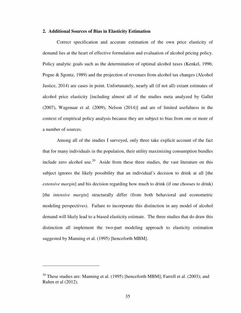
2. Additional Sources of Bias in Elasticity Estimation

Correct specification and accurate estimation of the own price elasticity of

demand lies at the heart of effective formulation and evaluation of alcohol pricing policy.

Policy analytic goals such as the determination of optimal alcohol taxes (Kenkel, 1996;

Pogue & Sgontz, 1989) and the projection of revenues from alcohol tax changes (Alcohol

Justice, 2014) are cases in point. Unfortunately, nearly all (if not all) extant estimates of

alcohol price elasticity [including almost all of the studies meta analyzed by Gallet

(2007), Wagenaar et al. (2009), Nelson (2014)] and are of limited usefulness in the

context of empirical policy analysis because they are subject to bias from one or more of

a number of sources.

Among all of the studies I surveyed, only three take explicit account of the fact

that for many individuals in the population, their utility maximizing consumption bundles

include zero alcohol use.20 Aside from these three studies, the vast literature on this

subject ignores the likely possibility that an individual’s decision to drink at all [the

extensive margin] and his decision regarding how much to drink (if one chooses to drink)

[the intensive margin] structurally differ (from both behavioral and econometric

modeling perspectives). Failure to incorporate this distinction in any model of alcohol

demand will likely lead to a biased elasticity estimate. The three studies that do draw this

distinction all implement the two-part modeling approach to elasticity estimation

suggested by Manning et al. (1995) [henceforth MBM].

20 These studies are: Manning et al. (1995) [henceforth MBM]; Farrell et al. (2003); and Ruhm et al (2012).

36

TJD et al. however, argue that the three aforementioned studies are themselves

subject to bias because, although the MBM elasticity measure takes explicit account of

both the extensive and intensive margins, it is not informative for alcohol pricing policy.

This lack of policy relevance of the MBM approach follows from the fact that it cannot

be placed in a potential outcomes framework and, as such, cannot be interpreted as

representing the causal relationship between price and alcohol consumption. TJD et al.

suggest an alternative elasticity specification (estimator) for the two-part context that is

derived within a potential outcomes framework that is causally interpretable.

In this section, I identify and detail additional sources of bias in TJD et al. (PO

method) and other extant approaches using two-part model (MBM method) to the

specification and estimation of the price elasticity of alcohol demand: 1) implementing a

restricted version of the two-part model (TJD et al.); 2) data aggregation that ignores the

extensive margin (AGG-LOG); and 3) the use of logged (vs. nominal) alcohol prices as a

matter of convenience (TJD et al. and AGG-LOG).

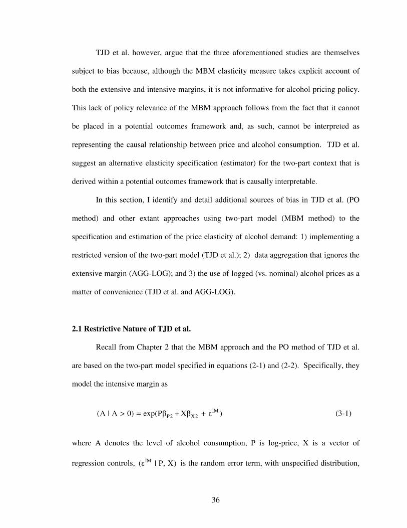
2.1 Restrictive Nature of TJD et al.

Recall from Chapter 2 that the MBM approach and the PO method of TJD et al.

are based on the two-part model specified in equations (2-1) and (2-2). Specifically, they

model the intensive margin as

IMP2 X2(A | A 0) exp(Pβ Xβ ε )> = + + (3-1)

where A denotes the level of alcohol consumption, P is log-price, X is a vector of

regression controls, IM(ε | P, X) is the random error term, with unspecified distribution,

37

defined such that IME[ε | P, X] 0= with IME[exp(ε ) | P, X] ψ= (a constant); and

2 P2 X2β = [β β ]′ ′ is the vector of parameters to be estimated. Consistent estimates of 1β

and 2β are obtained using the following two-part protocol.

The intensive margin as given in (3-1) is, however, unnecessarily restrictive.

Neither the explicit inclusion of IMε therein nor its accompanying conditional mean

assumptions are necessary. They are imposed merely as a matter of convenience – so

that the regression parameters P Xβ [β β ]′ ′= can be estimated via OLS. Instead, we

need only assume that

[ ] P2 X2E A | P, X, A > 0 exp(Pβ Xβ )= + . (3-2)

and the relevant regression parameters can still be estimated by applying the nonlinear

least squares (NLS) estimation method directly to (3-2).

This difference in assumptions is not trivial. Assumption (3-2) encompasses a

broader class of models than the conventional intensive margin specification given in (3-

1). Therefore, the conventional two-part model may be subject to misspecification bias.

As a result, in general, causal effect estimators cast in the conventional two-part

modeling framework, POη in particular, may be biased.

2.2 Log-Linear Models with Aggregated Data: Ignoring the Extensive Margin

The most widely implemented approach to estimation of the own-price elasticity

of the demand for alcohol is applying the ordinary least squares (OLS) method to a linear

demand model to an aggregated level dataset with log consumption as the dependent

38

variable and log price and other demand determinants as the independent variables

(henceforth the aggregate LOG method [AGG-LOG]). This includes a majority of the

aggregate-level studies covered by the meta analyses by Wagenaar et al. (2009), Nelson

(2014) and Gallet (2007).21 Here the OLS estimate of the regression coefficient of log

price is taken as the elasticity estimate. Its popularity notwithstanding, I argue that AGG-

LOG is potentially biased for analyzing pricing policies aimed at modifying alcohol

demand behavior at the individual level because it ignores individual alcohol demand

decisions at the extensive margin. The AGG-LOG model of the demand for alcohol is

expressed as

P XA exp(Pπ Xπ ξ)= + + . (3-3)

where A denotes the observed level of alcohol consumption, P is logged alcohol price,

and X is a vector of other alcohol demand determinants (controls); all of which are

measured at an aggregated level (e.g. averages at the level of the county, state, etc.). The

vector of regression parameters to be estimated is P Xπ [π π ]′ ′= and ξ is the random

term defined such that E ξ | P, X 0 = . In this case, it is easy to show that own-price

elasticity of alcohol demand is Pπ -- the coefficient of P in (3-3) [ ALPη π= ]. Under

these assumptions Pπ can be easily estimated by applying the OLS estimator to the

following log-log version of (3-3)

21 Almost all aggregate-level studies in Wagenaar et al. (2009) meta-analysis, at least 169 out of 191 beer elasticity estimates from meta-analysis by Nelson (2014), and 974 out of 1,172 alcohol elasticity estimates meta-analyzed by Gallet (2007) uses either Double-Log or System (Almost Ideal Demand System, Rotterdam) models, which ignore the extensive margins.

39

p Xln(A) Pπ Xπ ξ= + + . (3-4)

Owing to its simplicity, this approach is widely implemented and results obtained

from it are often used to analyze pricing policies aimed at modifying alcohol demand

behavior at the individual level. If, however, the population from which the aggregated

quantities A , P and X are drawn includes a nontrivial proportion of non-drinkers, and

the distinction between the extensive and intensive margins is important, in which case

individual level demand behavior may be more accurately characterized by a two-part

model, then this AGG-LOG approach is likely to be biased because it ignores this

distinction.

2.3 Using Log vs. Nominal Prices

Nearly all of the conceptual and empirical treatments of alcohol demand elasticity

found in the literature use log-price rather than nominal price. This is also true of TJD et

al. in the development of their causally interpretable elasticity measure, POη .22 The

origin of this practice traces to the convenience it affords via the log-log OLS (AGG-

LOG) model discussed in the previous section. There is, however, no substantive reason

for using log-price vs. nominal price and imposing this restriction on the model may lead

to bias.

22 TJD et al. specified their model using log price to conform to the extant literature.

40

3. An Alternative Elasticity Specification and Estimator

In the previous section I point out the lack of causal interpretability of the MBM

approach to elasticity specification and estimation (discussed in detail in TJD et al.) and

identify three additional potential sources of bias in extant elasticity measures and

estimators (including TJD et al.): 1) data aggregation that ignores the extensive margin

(AGG-LOG); 2) implementing a restricted version of the two-part model (TJD et al.);

and 3) the use of logged (vs. nominal) alcohol prices as a matter of convenience (TJD et

al. and AGG-LOG). In this section, I introduce a new approach to alcohol demand

elasticity specification and estimation that extends the PO model of TJD et al. so as to

avoid the three aforementioned biases. Table 3.1 summarizes various extant alcohol

elasticity estimators used by empirical researchers in the published literature and the

potential bias arising from each of them. An overwhelming majority of the extant

literature meta-analyzed by Wagenaar et al. (2009) [81.4% elasticity estimates], Nelson

(2014) [88.5% elasticity estimates] and Gallet (2007) [86.35% elasticity estimates] uses

the AGG-LOG model to estimate the price elasticity of alcohol demand in aggregated

data settings.23 Unfortunately, the extensive margin is ignored in all of these studies;

therefore, the policies implemented using these AGG-LOG elasticity estimates are

subject to bias.

23 These AGG-LOG elasticity estimates from the extant literature include double-log model and system models (such as the Almost Ideal Demand System (AIDS) and Rotterdam modeling approaches) when applied to aggregated data. The studies using system models allocate consumer expenditure from disposable income to different categories (such as alcohol, cigarettes, food, etc.) or its sub-categories. Using the aggregate data, the (log of) share of the expenditure on alcohol relative to total expenditure is then regressed on the log of a retail price index and other covariates to compute the (semi-) elasticity of alcohol.

41

I begin by specifying the following unrestricted version of the two part model

given in (1) and (2). This unrestricted model is cast in terms of nominal rather that log

prices:

Extensive Margin

A > 0 iff EMNOM1 X1I( a Xa e 0)+ + >PP (3-5)

where P is nominal price, EMNOM(e | , X)P is a logistically distributed random error term

and 1 1 X1a = [a a ]′ ′P is the vector of parameters to be estimated.

Intensive Margin

IMNOM2 X2(A | A 0) exp( a Xa e )> = + +PP (3-6)

where 2 2 X2a = [a a ]′ ′P is the vector of parameters to be estimated and

IMNOM(e | , X)P

is the random error term, with unspecified distribution, defined such that

[ ] 2 X2E A | , X, A > 0 exp( a Xa )= +PP P . (3-7)

Consistent estimates of 1a and 2a are obtained using the following unrestricted two-part

protocol.

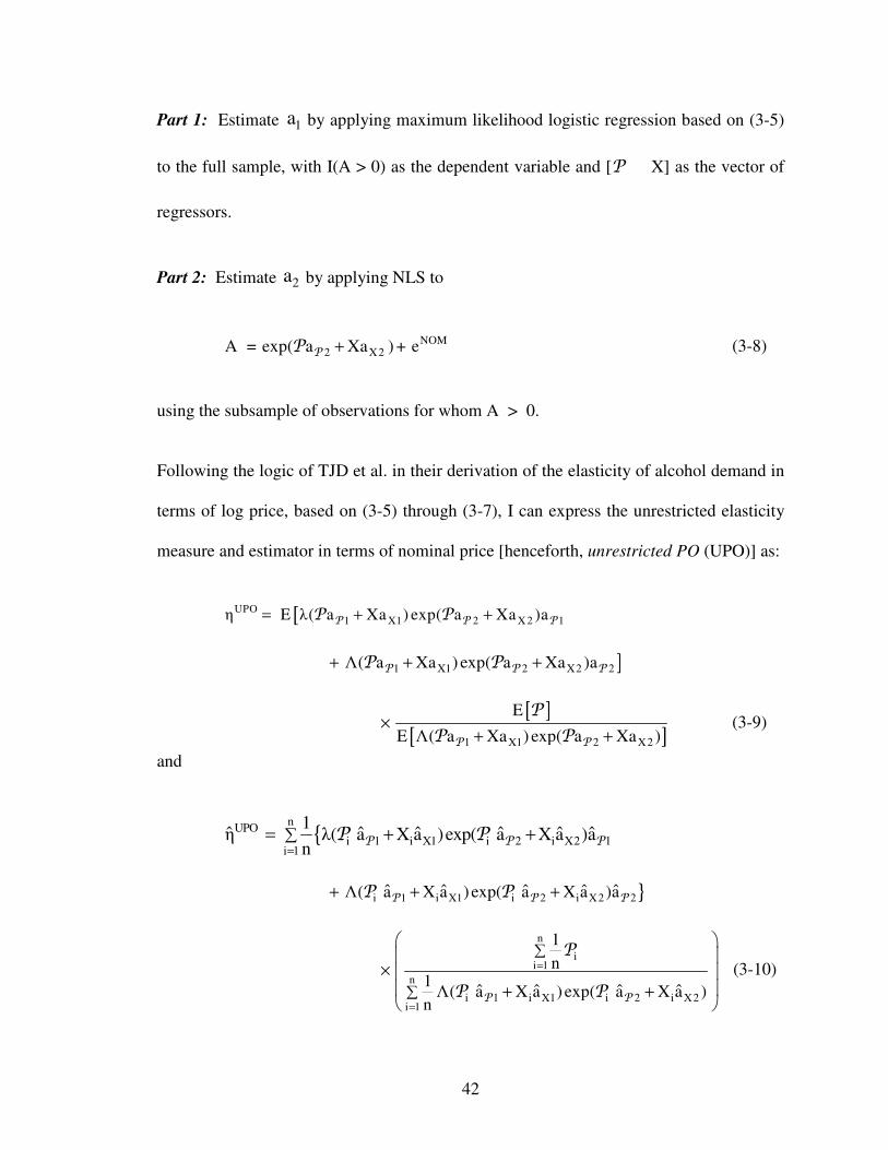
42

Part 1: Estimate 1a by applying maximum likelihood logistic regression based on (3-5)

to the full sample, with I(A > 0) as the dependent variable and [P X] as the vector of

regressors.

Part 2: Estimate 2a by applying NLS to

NOM2 X2A = exp( a Xa ) + e+PP (3-8)

using the subsample of observations for whom A > 0.

Following the logic of TJD et al. in their derivation of the elasticity of alcohol demand in

terms of log price, based on (3-5) through (3-7), I can express the unrestricted elasticity

measure and estimator in terms of nominal price [henceforth, unrestricted PO (UPO)] as:

[UPO1 X1 2 X 2 1η E λ( a Xa ) exp( a Xa )a= + +P P PP P

]1 X1 2 X2 2Λ( a Xa ) exp( a Xa )a+ + +P P PP P

[ ]

[ ]1 X1 2 X2

E

E Λ( a Xa ) exp( a Xa )×

+ +P P

P

P P (3-9)

and

n

UPOi 1 i X1 i 2 i X2 1

i 1

1ˆ ˆ ˆ ˆ ˆ ˆη λ( a X a )exp( a X a )a

n=∑= + +P P PP P

i 1 i X1 i 2 i X2 2ˆ ˆ ˆ ˆ ˆΛ( a X a )exp( a X a )a+ + +P P PP P

n

ii 1

n

i 1 i X1 i 2 i X2i 1

1

n1

ˆ ˆ ˆ ˆΛ( a X a ) exp( a X a )n

=

=

∑

∑

× + +

P P

P

P P

(3-10)

43

where 1 1 X1ˆ ˆ ˆa = [a a ]′ ′

P and 2 2 X2ˆ ˆ ˆa = [a a ]′ ′

P are the unrestricted two-part estimates

described above. The correct asymptotic standard error of (3-10) is derived in Appendix

E. Similar to the PO elasticity specification and estimator, UPOη and

UPOη are founded

in a potential outcomes framework that is causally interpretable (see TJD et al.).

Therefore, (3-10) produces elasticity estimates that are causally interpretable and, as

such, are useful for policy analysis. In the section 4, I use simulated and real data, to

compare results obtained using UPOη (our preferred estimator) to those from the most

commonly used extant method discussed in section 2, viz., AGG-LOG (ALη ).

4. Bias from using AGG-LOG method Ignoring the Extensive Margin and the UPO

In Appendix F, I show that the difference between ALη and

UPOη (the bias from

implementing ALη instead of the

UPOη ) can be expressed as:

AL UPOP 1

uη η π 1 a a m

v

− = − − +

P P2 P (3-11)

where24

1 2v E[Λ(Wa )exp(Wa )]≡ (3-12)

21 2u E[Λ(Wa ) exp(Wa )]≡ (3-13)

24 The expected values are with respect to W .

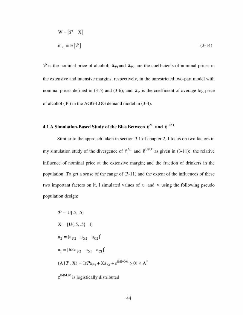
44

[ ]W X= P

[ ]m E≡P P (3-14)

P is the nominal price of alcohol; 1aP and 2aP are the coefficients of nominal prices in

the extensive and intensive margins, respectively, in the unrestricted two-part model with

nominal prices defined in (3-5) and (3-6); and Pπ is the coefficient of average log price

of alcohol ( P ) in the AGG-LOG demand model in (3-4).

4.1 A Simulation-Based Study of the Bias Between ALη and

UPOη

Similar to the approach taken in section 3.1 of chapter 2, I focus on two factors in

my simulation study of the divergence of ALη and

UPOη as given in (3-11): the relative

influence of nominal price at the extensive margin; and the fraction of drinkers in the

population. To get a sense of the range of (3-11) and the extent of the influences of these

two important factors on it, I simulated values of u and v using the following pseudo

population design:

~ U.5, .5P

X [U.5, .5 1]=

2 2 X2 C2a [a a a ]′= P

1 2 X1 C1a [h a a a ]′= × P

IMNOM *1 X1(A | , X) I( a Xa e 0) A= + + > ×PP P

IMNOMe is logistically distributed

45

*2 X2(A | , X) ~ gamma(exp( a Xa ),1)+PP P (3-15)

where Um, v denotes the uniform random variable with mean m and variance v,

gamma(sh,sc) denotes the gamma random variable with shape parameter sh and scale

parameter sc, 2aP is the coefficient of nominal price in the second part of the unrestricted

two-part model (intensive margin), Xja and Cja (j = 1 [extensive], 2 [intensive]) are the

coefficient of the control variable and the constant term, respectively, for each of the

parts of the model, and h is a factor representing the relative influence of nominal price

on the extensive margin vs. the intensive margin (0 ≤ h ≤ ∞). A is assumed to be a

gamma random variable so that it does not conform to the restrictions imposed by the

restricted two-part model. The bigger is h, the greater the relative influence of nominal

price on the extensive vs. the intensive margin. The “true” values of v , u and mP for

this simulated population design were obtained by generating a “super sample” of 2

million values (n* = 2000K) for W and A based on the sampling design in (3-15) and

then evaluating

n*

i* 1 i* 2i* 1

1v Λ(W a )exp(W a )

n *=∑≡

n*

2i* 1 i* 2

i* 1

1u Λ(W a ) exp(W a )

n *=∑≡

and

n*

ii* 1

1m )

n *=∑≡P P

respectively. To get the true value of Pπ I first equally split the super sample into 50

arbitrary states. I then aggregate the simulated data at to the state-level by taking the

46

means of A and X, represented by A and X respectively. The nominal prices, P are first

averaged across states and that mean is logged to get P . OLS is then applied to (3-4)

using the super sample and the estimated coefficient of P ( Pπ ) is taken as the true value

of Pπ because

P Pˆπ plim(π )= .25

To investigate the nature of the bias, I varied h and C1a with 2aP , X2a and X1a all

set equal to -1; and C2a is set equal to 1. By increasing h, I increased the relative

influence of nominal price at the extensive margin (vis-a-vis the intensive margin).

Ceteris paribus increases in C1a correspond to increases in the fraction of drinkers in the

population. The values of the nominal bias (3-11) corresponding to a variety of (h, C1a )

pairs are given in Table 3.2 along with the bias as a percentage of UPOη (in parentheses) -

- a measure of relative bias. In each cell I also report the fraction of drinkers in the

population [in brackets].

I first note that the nominal values of bias in Table 3.2 are uniformly positive for

almost all combinations of h and C1a . It is also evident from the Table 3.2 that for any

given value of C1a the absolute values of both nominal and percentage bias

monotonically increases as h increases. Also, for a given value of h, the absolute values

of bias vary upwards and then downwards when the fraction of drinkers increases. Note

25 plim is short for “probability limit” which is a large sample (n approaches infinity) desirable statistical property of an estimator analogous to unbiasedness, the desirable small (or finite) sample property.

47

that the bias can get quite large even for reasonable levels of h and the population

proportion of drinkers – e.g. at h=1 and proportion of drinkers=58.53% ( C1a 3= ) the bias

is 30.54%.

4.2 Comparison of ALη and UPOη with Real Data

As a means of demonstrating the potential empirical consequences of ignoring the

extensive margin, I estimate own price elasticity by applying both the ALη and the

UPOη

estimation protocols to the following demand specification

A = average daily volume of ethanol consumption from beer in ounces during the

past year

P = Nominal price of beer in $ per ounce of ethanol

X = [gender, marital status, age, race, household income, family size, education,

region of residence, and occupation]

where variables and datasets are defined in section 3.2 of Chapter 2.

I then construct the artificially aggregated data by first taking the mean of the

dependent variable (average daily volume of ethanol from beer in ounces) and the

observable confounders (such as gender, marital status, age, race, household income,

family size, and education) across all observations in each state. The UPC price data was

already available at a state-level, measured in weighted price per ounce of ethanol. The

mean of nominal price and actual consumption across observations at the state level were

then logged as a precursor to the implementation of the AGG-LOG method. This

artificial state-level aggregated database was then used to estimate the price elasticity of

alcohol demand using the AGG-LOG method detailed in the section 2.2 of this chapter.

48

The summary statistics of this artificially aggregated state-level database are presented in

Table 3.3.

Our focus here is on the size and statistical significance of ALη ,

UPOη and their

difference AL UPOˆ ˆη η− . The standard error of

UPOη is derived in Appendix E and that of

the difference statistic for the bias, AL UPOˆ ˆη η− , is derived in Appendix G. Table 3.4

shows the comparison of the AGG-LOG and UPO elasticity estimators for the price of

beer. The first column presents the elasticity estimate ALη , obtained using the parameter

estimation protocol in equation (3-4). The second column of Table 3.4 shows UPOη , the

elasticity estimate in equation (3-10) obtained using the two-part protocol culminating in

equation (3-8). For the demand specification with all controls, I find the AGG-LOG

elasticity estimate is -0.7136 and insignificant, but the UPO estimate was -0.5057 and

statistically significant at 5% level. The difference between AGG-LOG and UPO was -

0.2079 and statistically insignificant for the demand specification with all controls.

However, for an alternate demand specification without the region of residence and

occupation as controls, I find the AGG-LOG estimate for beer is -0.8966 and was

insignificant, whereas the UPO estimate is -0.4902 and was significant at 1% level. The

difference between the AGG-LOG and the UPO estimates is -0.4064 and significant at

5% level. It should be noted that the elasticity estimate obtained using the UPO model is

statistically significant in both demand specifications, implying that it is imperative to

take into account the extensive margins, which AGG-LOG ignores. The percentage

discrepancy between the AGG-LOG and UPO elasticity estimates is 82.91%.

In both the simulation and real data analyses, I find strong evidence of biased

49

estimates from ignoring the extensive margin in price elasticity of alcohol demand. In

the following, I examine how such differences may translate to the assessment of

potential revenue generation from changes in alcohol taxes.

4.3 Revenue Generation from Tax Changes

As discussed in section 3.3 of Chapter 2, alcohol elasticities can also be used to

estimate the potential change in revenues that would result from an increase in taxes.

Therein, I also detail the simple revenue generation model developed by Alcohol Justice

(2014), an organization that leads campaigns for raising alcohol taxes to fund government

programs. Combining the Alcohol Justice model with the elasticities obtained by

applying the AGG-LOG method to the artificially aggregated version of the data from

Ruhm et al. (2012), I forecast the change in revenue that would result from a proposal to

increase the Federal excise tax on alcohol by Congressional Budget Office (CBO) [See

section 3.3 of Chapter 2 for details]. Table 3.5 shows the results for the revenue

generation forecasts based on both the AGG-LOG and the UPO elasticity estimates

obtained in section 4.3 (viz.,UPOη 0.4902= − and ALη 0.8966= − ). The difference is

substantial, amounting to a $207.1 million per year shortfall for the former. Such

forecasting mistakes could result in serious errors in budget appropriation. In this

example, the discrepancy is equal to 46.3% of the budget for the National Institute of

Alcohol Abuse and Alcoholism (NIAAA) in Fiscal Year 2015.

50

5. Summary and Conclusion

In this chapter, I introduced a specification of the price elasticity of alcohol

demand [UPOη in equation (3-9)] and its corresponding consistent estimator [

UPOη in

equation (3-10)] that takes into account the extensive margin, is founded in a potential

outcomes framework that is causally interpretable, uses nominal prices of alcohol instead

of logged price and relaxes the unnecessarily restrictive assumptions underlying the

conventional two-part model. To examine the extent of the bias between the widely used

AGG-LOG method vs. the UPO method, I performed a simulation study, where I varied

the relative influence of nominal price at the extensive margin and the fraction of drinkers

in the population. I found uniformly positive and substantial bias for almost all

combinations and for a given level of former, as latter increases the bias monotonically

increases. I also applied both methods to the dataset analyzed by Ruhm et al. (2012) and

found the elasticity estimates to be statistically different from each other (

AL UPOˆ ˆη η 0.4064− = − ; p-value=0.0277) for a particular demand specification. Such

differences are profound when placed in the context of revenue generation. The

difference between the approaches in terms of projected revenue for a recently proposed

federal excise tax increase for beer was $207.1 million per year, which is 46.3% of the

yearly budget of the NIAAA.

51

Table 3.1: Summary of extant alcohol elasticity estimators and additional biases

Econometric Models

Accounts for

extensive margin

Studies using

Nominal prices

instead of Log

Unrestricted version of the

two-part model

Causally Interpretable

Percentage or # of

elasticity studies

AGG-LOG Models No Mixed NA Yes

W=81.40% N=88.47% G=86.36%

Tobit No No NA Maybe 1 study

Finite Mixture Models

No No NA Maybe 2 studies

2PM – MBM Yes No No No 3 studies

2PM – TJD et al.

Yes No No Yes 1 study

2PM – This paper

Yes Yes Yes Yes -

NA =Not applicable

Wagenaar et al. (2009) [W], Nelson (2014) [N], Gallet (2007) [G]

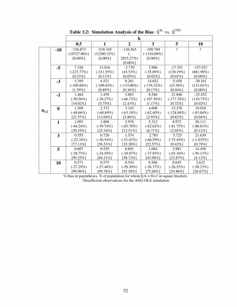
52

Table 3.2: Simulation Analysis of the Bias: ALη vs.

UPOη

h

0.5 1 2 3 5 10

C1a

-10 -336.873 (10727.96%)

[0.00%]

-518.345 (12380.32%)

[0.00%]

-126.565 (-

2015.27%) [0.00%]

-109.704 (-1310.09%)

[0.00%]

†

†

-5 7.326 (-233.77%)

[0.23%]

13.016 (-311.55%)

[0.12%]

-2.730 (43.53%) [0.05%]

2.986 (-35.69%) [0.02%]

-17.351 (138.19%) [0.01%]

-157.021 (681.90%)

[0.00%]

-3 3.395 (-109.66%)

[1.59%]

4.521 (-109.65%)

[0.89%]

8.261 (-133.06%)

[0.36%]

14.652 (-176.32%)

[0.17%]

-5.458 (43.58%) [0.04%]

-30.161 (131.01%)

[0.00%]

-1 1.464 (-50.56%) [10.02%]

1.459 (-38.27%) [5.75%]

3.883 (-66.72%) [2.43%]

8.546 (-107.56%)

[1.17%]

21.846 (-177.76%)

[0.32%]

-25.452 (110.75%)

[0.02%]

0 1.309 (-48.66%) [21.57%]

2.372 (-68.69%) [13.04%]

3.343 (-63.18%) [5.86%]

4.608 (-62.40%) [2.93%]

15.278 (-128.68%)

[0.82%]

19.018 (-83.04%) [0.04%]

1 1.093 (-44.24%) [39.19%]

1.806 (-59.74%) [25.34%]

2.976 (-65.78%) [12.51%]

5.312 (-82.62%) [6.71%]

8.972 (-81.75%) [2.05%]

20.111 (-88.63%) [0.12%]

3 0.555 (-25.34%) [77.11%]

0.728 (-30.54%) [58.53%]

1.574 (-51.03%) [35.20%]

2.785 (-66.59%) [22.57%]

5.725 (-75.44%) [9.42%]

21.639 (-1.035%) [0.79%]

5 0.607 (-28.75%) [95.25%]

0.529 (-24.58%) [84.21%]

0.691 (-28.87%) [58.72%]

1.084 (-37.85%) [42.90%]

2.983 (-65.16%) [23.87%]

14.458 (-95.13%) [4.12%]

10 0.571 (-27.29%) [99.96%]

0.575 (-27.46%) [99.76%]

0.554 (-26.30%) [91.58%]

0.568 (-26.37%) [75.68%]

0.645 (-26.52%) [54.86%]

2.632 (-58.23%) [26.67%]

%-bias in parentheses, % of population for whom I(A > 0)=1 in square brackets. †Insufficient observations for the AGG-OLS simulation

53

Table 3.3: Summary Statistics of Artificially Aggregated Data

Variable Name Description Mean

N=35 Std.Dev

Average Alcohol Consumption if Drinker

Average Daily ethanol from beer in ounces

0.1639 0.0430

log of Average Alcohol Consumption

Log of Average oz of daily ethanol from beer

-1.8418 0.2647

Price Logged price of beer per oz of

ethanol from UPC barcode data 0.1877 0.0808

X Variables

female Average share of females 0.5775 0.0282

married Share of sample who are currently

married 0.5043 0.0563

lnage Log of (average age) 3.8117 0.0565

black Share of Black population in the

sample 0.2226 0.1705

hispanic Share of sample who are Hispanic

origin 0.1430 0.1397

other Share of sample with other race 0.0395 0.0246

lnincome Log of (average household

income) 10.5434 0.1525

lnfamsize Log of (Average Family size) 0.7953 0.0570

nohs Share of sample with no high

school 0.1447 0.0375

somecllg Share of sample with some college

attendance 0.3157 0.0374

college Share of sample who have

completed college 0.2748 0.0650

54

Table 3.4: Comparing ALη vs. UPOη Method Using Real Data

Demand

Specification ALη

UPOη

Difference, AL UPOˆ ˆη η−

% Difference AL UPO

UPO

ˆ ˆη η100%

η

−×

With all controls

-0.7136 (-0.7623)

-0.5057** (-2.1309)

-0.2079 (-0.8663)

41.11%

Without region of

residence and occupation as

controls

-0.8966 (-1.0934)

-0.4902*** (-2.6907)

-0.4064** (-2.2017)

82.91%

T-statistics in parenthesis. * p<0.10, ** p<0.05, *** p<0.01

55

Table 3.5: Results of Changes in Tax Revenues from Federal Excise Tax Increase

Description

Change in tax

revenues using ALˆη η=

(a)

Change in tax

revenues using UPOˆη η=

(b)

Difference

(a) – (b)

nominal dollars

Additional revenues from “proposed” federal excise tax increase

$4.921 billion $5.128 billion -$207.064 million

56

Chapter 4.

Specification and Estimation of Alcohol Price Elasticity in Individual-Level Demand

Models Using Nominal vs. Log Prices

1. Introduction

Chapters 2 and 3, respectively, assess possible empirical consequences (bias)

from implementing elasticity specifications and estimators that are not causally

interpretable; or do not take account of individual alcohol demand decisions made at the

extensive margin; or implements unnecessarily restrictive version of the two-part model.

The results demonstrate that these modeling deficiencies can lead to substantial

divergence from elasticity estimates obtained via an approach that is both causally

interpretable, explicitly models the extensive margin, are least restrictive and uses

nominal prices of alcohol. Moreover, the prior chapters show that these differences can

translate to nontrivial differences in associated policy recommendations in the context of

revenue generation. To remain consistent with existing literature, however, in Chapter 2,

I cast the elasticity specifications, estimators, and comparisons thereof, in terms of log of

prices instead of nominal prices. Recall that in Chapter 3, I develop the UPO approach to

alcohol demand elasticity specification and estimation which is free of biases including

the use of nominal prices. Majority of the extant literature on alcohol elasticity uses

logged prices of alcohol instead of nominal prices. Other than the need to conform to

extant literature, there is no clear reason to formulate alcohol demand models and their

corresponding elasticity measures in terms of log vs. nominal prices.

In the present chapter, to investigate the empirical consequences of modeling

alcohol demand in terms of log vs. nominal prices, I develop a version of the UPO

57

method for elasticity specification and estimation (detailed in Chapter 3) that is cast in

terms of logged prices. I will henceforth refer to this approach as the UPOL method.

Using simulated and real data from Ruhm et al. (2012), I apply the UPOL method and

compare the results with the corresponding elasticity estimates obtained using the UPO

method and reported in Chapters 3. I then evaluate how differences in the elasticity

estimates (UPOL vs. UPO) translate to differences in revenue generation. I find

reasonable differences in estimates of alcohol price elasticity. These differences are more

pronounced when placed in the revenue generation policy making contexts.

This chapter is structured as follows. The next section will detail the UPOL

method for elasticity specification and estimation. In section 3, I will compare the UPOL

with the UPO methods using simulated data and a real analysis sample from the Ruhm et

al. (2012) study. I also discuss the data and results in detail. The comparison of elasticity

estimates in the context of a change in beer tax revenues are also given therein. The final

section summarizes and concludes the chapter.

2. Unrestricted PO Elasticity Specification and Estimator with logged prices

In the previous section I point out that nearly all of the conceptual and empirical

treatments of alcohol demand elasticity found in the literature use log-price rather than

nominal price. This is also true of TJD et al. in the development of their causally

interpretable elasticity measure, POη , the MBM model, and most studies using AGG-

LOG models.26 The origin of this practice traces to the convenience it affords via the

log-log OLS (AGG-LOG) model discussed in the previous section. There is, however,

26 TJD et al. specified their model using log price to conform to the extant literature.

58

no substantive reason for using log-price vs. nominal price and imposing this restriction

on the model may lead to bias. In Chapter 3, I develop the UPO model that takes explicit

account of extensive margin, are causally interpretable, uses unrestricted version of two-

part model, and uses nominal prices in the own price elasticity of alcohol demand

specification and estimation. In this section, I introduce a version of UPO approach in

which the prices are cast as logged prices (UPO approach). I begin by specifying the

following unrestricted version of the two part model cast in nominal prices given in (1)

and (2).

Extensive Margin

A > 0 iff EMLOGP1 X1I(Pα Xα e 0)+ + > (4-1)

where P is logged price, EMLOG(e | P, X) is a logistically distributed random error term

and 1 P1 X1α = [α α ]′ ′ is the vector of parameters to be estimated.

Intensive Margin

IMLOGP2 X2(A | A 0) exp(Pα Xα e )> = + + (4-2)

where 2 P2 X2α = [α α ]′ ′ is the vector of parameters to be estimated and IMLOG(e | P, X)

is the random error term, with unspecified distribution, defined such that

[ ] P2 X2E A | P, X, A > 0 exp(Pα Xα )= + . (4-3)

59

Consistent estimates of 1α and 2α are obtained using the following unrestricted two-part

protocol.

Part 1: Estimate 1α by applying maximum likelihood logistic regression based on (4-1)

to the full sample, with I(A > 0) as the dependent variable and [P X] as the vector of

regressors.

Part 2: Estimate 2α by applying NLS to

LOGP2 X2A = exp(Pα Xα ) + e+ (4-4)

using the subsample of observations for whom A > 0.

Following the logic of TJD et al. in their derivation of the elasticity of alcohol demand in

terms of log price, based on (4-1) through (4-3), I can express the unrestricted elasticity

measure and estimator in terms of logged price [henceforth, unrestricted PO with logged

prices (UPOL)] as:

[UPOLP1 X1 P2 X 2 P1η E λ(P α Xα ) exp(P α Xα )α= + +

]P1 X1 P2 X2 P2Λ(Pα Xα ) exp(Pα Xα )α+ + +

[ ]P1 X1 P2 X2

1

E Λ(Pα Xα ) exp(Pα Xα )×

+ + (4-5)

and

n

UPOLi P1 i X1 i P2 i X2 P1

i 1

1ˆ ˆ ˆ ˆ ˆ ˆη λ(P α X α )exp(P α X α )α

n=∑= + +

i P1 i X1 i P2 i X2 P2ˆ ˆ ˆ ˆ ˆΛ(P α X α ) exp(P α X α )α+ + +

60

n

i P1 i X1 i P2 i X2i 1

1

1ˆ ˆ ˆ ˆΛ(P α X α ) exp(P α X α )

n=∑

× + +

(4-6)

where 1 P1 X1ˆ ˆ ˆα = [α α ]′ ′ and 2 P2 X2

ˆ ˆ ˆα = [α α ]′ ′ are the unrestricted two-part estimates

described above. The correct asymptotic standard error of (4-6) is derived in Appendix H.

Similar to the UPO elasticity specification and estimator, UPOLη and

UPOLη are founded

in a potential outcomes framework that is causally interpretable (see TJD et al. and

Chapter 3), however, it uses logged prices instead of nominal prices. Therefore, (4-6)

produces elasticity estimates that are causally interpretable, but may be subjected to bias,

hence may not be useful for policy analysis. In the section 3, I use simulated and real

data, to compare results obtained using UPOLη to

UPOη (our preferred estimator obtained

and discussed in Chapter 3).

3. Bias from using the UPOL method and the UPO

In Appendix I, I show that the difference between UPOLη and

UPOη (the bias from

implementing UPOLη instead of the

UPOη ) can be expressed as:

UPOL UPOP1 P2 1 2

ω uη η 1 α α 1 a a m

ν v

− = − + − − +

P P P (4-7)

where27

27 The expected values are with respect to W for nominal prices and W

for logged prices.

61

1 2ν E[Λ(Wα ) exp(W α )]≡

(4-8)

21 2ω E[Λ(W α ) exp(W α )]≡

(4-9)

1 2v E[Λ(Wa )exp(Wa )]≡ (4-10)

21 2u E[Λ(Wa ) exp(Wa )]≡ (4-11)

[ ]W P X=

[ ]W X= P

[ ]m E≡P P (4-12)

P is the nominal price of alcohol; P is the logged price of alcohol; P1α and P2α are the

coefficients of logged prices in the extensive and intensive margins, respectively, in the

unrestricted two-part model with nominal prices defined in equations (4-1) and (4-2) of

this chapter; and 1aP and 2aP are the coefficients of nominal prices in the extensive and

intensive margins, respectively, in the unrestricted two-part model with nominal prices

defined in equations (3-5) and (3-6) of Chapter 3.

3.1 A Simulation-Based Study of the Bias Between UPOLη and

UPOη

I focus on the relative influence of nominal price at the extensive margin in my

simulation study of the divergence of UPOLη and

UPOη as given in (4-7). To get a sense of

the range of (4-7) and the extent of the influences of this important factor on it, I

simulated values of u and v using the following pseudo population design:

62

~ U.5, .5P

X [U.5, .5 1]=

2 2 X2 C2a [a a a ]′= P

1 2 X1 C1a [h a a a ]′= × P

IMNOM *1 X1(A | , X) I( a Xa e 0) A= + + > ×PP P

IMNOMe is logistically distributed

*2 X2(A | , X) ~ gamma(exp( a Xa ),1)+PP P (4-13)

where Um, v denotes the uniform random variable with mean m and variance v,

gamma(sh,sc) denotes the gamma random variable with shape parameter sh and scale

parameter sc, 2aP is the coefficient of nominal price in the second part of the unrestricted

two-part model (intensive margin), Xja and Cja (j = 1 [extensive], 2 [intensive]) are the

coefficient of the control variable and the constant term, respectively, for each of the

parts of the model, and h is a factor representing the relative influence of nominal price

on the extensive margin vs. the intensive margin (0 ≤ h ≤ ∞). A is assumed to be a

gamma random variable so that it does not conform to the restrictions imposed by the

restricted two-part model. The bigger is h, the greater the relative influence of nominal

price on the extensive vs. the intensive margin. The “true” values of v , u and mP for

this simulated population design were obtained by generating a “super sample” of 2

million values (n* = 2000K) for W and A based on the sampling design in (4-13) and

then evaluating

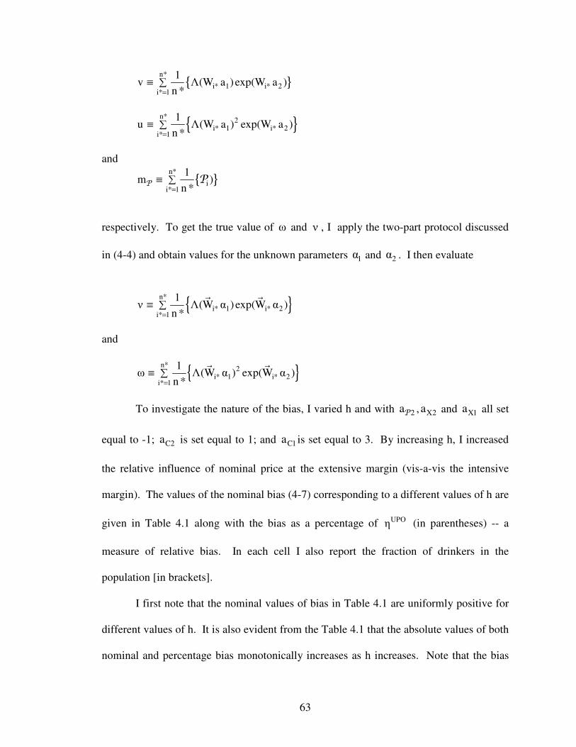
63

n*

i* 1 i* 2i* 1

1v Λ(W a )exp(W a )

n *=∑≡

n*

2i* 1 i* 2

i* 1

1u Λ(W a ) exp(W a )

n *=∑≡

and

n*

ii* 1

1m )

n *=∑≡P P

respectively. To get the true value of ω and ν , I apply the two-part protocol discussed

in (4-4) and obtain values for the unknown parameters 1α and 2α . I then evaluate

n*

i* 1 i* 2i* 1

1ν Λ(W α ) exp(W α )

n *=∑≡

and

n*

2i* 1 i* 2

i* 1

1ω Λ(W α ) exp(W α )

n *=∑≡

To investigate the nature of the bias, I varied h and with 2aP , X2a and X1a all set

equal to -1; C2a is set equal to 1; and C1a is set equal to 3. By increasing h, I increased

the relative influence of nominal price at the extensive margin (vis-a-vis the intensive

margin). The values of the nominal bias (4-7) corresponding to a different values of h are

given in Table 4.1 along with the bias as a percentage of UPOη (in parentheses) -- a

measure of relative bias. In each cell I also report the fraction of drinkers in the

population [in brackets].

I first note that the nominal values of bias in Table 4.1 are uniformly positive for

different values of h. It is also evident from the Table 4.1 that the absolute values of both

nominal and percentage bias monotonically increases as h increases. Note that the bias

64

can get quite large even for reasonable levels of h and the population proportion of

drinkers – e.g. at h=1 and proportion of drinkers=58.53%, the bias is 44.87%.

3.2 Comparison of UPOLη and UPOη with Real Data

As a means of demonstrating the potential empirical consequences of ignoring the

extensive margin, I estimate own price elasticity by applying both the UPOLη and the

UPOη estimation protocols to the following demand specification

A = average daily volume of ethanol consumption from beer in ounces during the

past year

P = Nominal price of beer in $ per ounce of ethanol

X = [gender, marital status, age, race, household income, family size, education,

region of residence, and occupation]

where variables and datasets are defined in section 3.2 of Chapter 2.

Our focus here is on the size and statistical significance of UPOLη ,

UPOη and their

difference UPOL UPOˆ ˆη η− . The standard error of

UPOη is derived in Appendix H and that

of the difference statistic for the bias, UPOL UPOˆ ˆη η− , is derived in Appendix J. Table 4.2

shows the comparison of the UPOL and UPO elasticity estimators for the price of beer.

The first column presents the elasticity estimate UPOLη , obtained using the parameter

estimation protocol in equation (4-4). The second column of Table 4.2 shows UPOη , the

elasticity estimate in equation (3-10) of chapter 3 obtained using the two-part protocol

culminating in equation (3-8) of chapter 3. I find the UPOL elasticity estimate is -0.4892

and statistically significant at 5% level. Recall from Chapter 3 that the UPO estimate was

65

-0.5057 and statistically significant at 5% level. The difference between the UPOL and

the UPO estimates is 0.0165, but statistically insignificant. Nevertheless, the absolute

percentage discrepancy between the UPOL and UPO elasticity estimates is 3.26%.

In both the simulation data analyses, I find strong evidence of biased estimates

from using logged prices instead of nominal prices. However, in real data settings, with

the demand specification used in Ruhm et al. (2012), I find suggestive evidence of bias.

In the following section, I examine how such differences may translate to the assessment

of potential revenue generation from changes in alcohol taxes.

3.3 Revenue Generation from Tax Changes

Combining the Alcohol Justice model (discussed in section 3.3 of chapter 2) with

the elasticities obtained by applying the UPOL method to the data from Ruhm et al.

(2012), I forecast the change in revenue that would result from a proposal to increase the

Federal excise tax on alcohol by Congressional Budget Office (CBO) [See section 3.3 of

Chapter 2 for details]. Table 4.3 shows the results for the revenue generation forecasts

based on both the UPOL and the UPO elasticity estimates obtained in section 4.2 (viz.,

UPOη 0.4902= − and UPOLη 0.5057= − ). The difference amount to a $8.4 million per

year shortfall for the former. Such forecasting mistakes could result in reasonable errors

in budget appropriation. In this example, the discrepancy is equal to 2% of the budget for

the National Institute of Alcohol Abuse and Alcoholism (NIAAA) in Fiscal Year 2015.

66

4. Summary and Conclusion

In this chapter, I compare the estimator of the price elasticity of alcohol demand [

UPOη in equation (3-10) of chapter 3] that uses nominal prices of alcohol instead of

logged price (and is free from other biases discussed in Chapter 3) with an estimator that

uses logged prices of alcohol in the demand specification [UPOLη in equation (4-6) of this

chapter]. To examine the extent of the bias between the UPOL vs. the UPO method, I

performed a simulation study, where I varied the relative influence of nominal price at

the extensive margin. I found uniformly positive and substantial bias for almost all

variations. I also applied both methods to the dataset analyzed by Ruhm et al. (2012) and

found suggestive evidence of smaller bias in the elasticity estimates (

UPOL UPOˆ ˆη η 0.0165− = , but insignificant). Such differences are reasonable when placed

in the context of revenue generation. The difference between the approaches in terms of

projected revenue for a recently proposed federal excise tax increase for beer was $8.4

million per year, which is 2% of the yearly budget of the NIAAA.

67

Table 4.1: Simulation Analysis of the Bias: UPOLη vs.

UPOη

h

0.5 1 2 3 5 10 1.002

(-45.75%) [77.11%]

1.069 (-44.87%) [58.53%]

1.512 (-49.04%) [35.20%]

2.278 (-54.47%) [22.57%]

4.708 (-62.04%) [9.42%]

14.51 (-69.38%) [0.79%]

%-bias in parentheses, % of population for whom I(A > 0)=1 in square brackets.

68

Table 4.2: Comparing UPOLη vs. UPOη Method Using Real Data

UPOLη UPOη

Difference, UPOL UPOˆ ˆη η−

% Difference UPOL UPO

UPO

ˆ ˆη η100%

η

−×

-0.4892** (-2.1284)

-0.5057** (-2.1309)

0.0165 (0.0498)

-3.26%

T-statistics in parenthesis. * p<0.10, ** p<0.05, *** p<0.01

69

Table 4.3: Results of Changes in Tax Revenues from Federal Excise Tax Increase

Description

Change in tax

revenues using UPOLˆη η=

(a)

Change in tax

revenues using UPOˆη η=

(b)

Difference

(a) – (b)

nominal dollars

Additional revenues from “proposed” federal excise tax increase

$5.129 billion $5.121 billion $8.41 million

70

Chapter 5.

Summary and Conclusion

1. Introduction

Several state legislatures in the US have imposed, or are considering increasing,

sumptuary or Pigouvian taxes (e.g., “sin taxes”) predominantly on alcohol and tobacco.

Such pricing policies are set so as to reduce the consumption of alcohol abusers so as to

minimize external costs to those harmed by them. There also has been growing interest

in raising alcohol excise taxes to increase government revenues to reduce budget deficits

or to fund various state and federal programs. The own-price elasticity of the demand for

alcohol plays a vital role in determining optimal Pigouvian taxes (to reduce externalities)

and in projecting revenues generated from proposed tax changes.28 Therefore, accurate

estimation of alcohol price elasticity is important for policy analysis.

2. Key Aspects of Policy Relevant Alcohol Elasticity Specification and Estimation

Many different approaches to specifying and estimating the price elasticity of

demand for alcohol can be found in the literature. There are four keys to policy-relevant

specification and estimation of alcohol price elasticity. First, the underlying demand

model should take account of alcohol consumption decisions at the extensive margin –

i.e., individuals’ decisions to drink or not – because the price of alcohol may impact the

drinking initiation decision. This is important because one’s decision to drink is likely to

be structurally different from how much they drink if they decide to do so (the intensive

28 See Chapter 1 of dissertation for details on the role of elasticities in the context of revenue generation.

71

margin). Secondly, the modeling of alcohol demand elasticity should yield both

theoretical and empirical results that are causally interpretable and, therefore, useful for

the analysis of potential changes in alcohol consumption that would result from

exogenous (and ceteris paribus) changes in the price of alcohol (e.g., a change in tax

policy). Thirdly, the extant models that explicitly take extensive margins into account are

unnecessarily restrictive and are merely imposed as a matter of convenience so that the

parameters can be estimated using the Ordinary Least Squares (OLS) method. Finally,

almost all the conceptual and empirical treatments of alcohol demand elasticity found in

the literature use log-price rather than nominal price.

There currently exists no specification and estimation method for alcohol price

elasticity that accommodates the extensive margin, is causally interpretable, is less

restrictive and uses nominal prices of alcohol. One of the primary goals of this

dissertation is to detail and evaluate a new approach to the specification and estimation of

alcohol price elasticity that covers these four key requirements for policy relevance.

2.1. Models that Account for the Extensive Margin

The vast majority of extant studies that I surveyed do not accommodate the

possibility that one’s decision to drink or not [extensive margin] may require special

attention in model design. If the relevant population includes a nontrivial proportion of

non-drinkers and the extensive margin is ignored in modeling then the resultant elasticity

measure is likely to be biased. The most widely implemented approach to estimation of

the own-price elasticity of the demand for alcohol is applying the ordinary least squares

(OLS) method to a linear demand model with log consumption as the dependent variable

72

and log price and other demand determinants as the independent variables [henceforth the

aggregate LOG method (AGG-LOG)] on aggregate-level (e.g. state-level) models and

data. Unfortunately, nearly all of these studies incapable of taking explicit account of

individual alcohol demand decisions at the extensive margin, therefore, elasticity

estimates obtained using AGG-LOG is potentially biased for analyzing pricing policies

aimed at modifying alcohol demand behavior at the individual level.29 The two-part

model developed by Manning, Blumberg, Moulton (1995) [MBM henceforth] to estimate

the own price elasticity of alcohol demand is indeed designed to account for the structural

difference between the extensive and intensive margins. Of all the alcohol elasticity

studies I surveyed, only three alcohol elasticity studies take explicit account of the

extensive margin by implementing the MBM approach (Manning et al., 1995; Farrell et

al., 2003; Ruhm et al., 2012).

2.2. Models that are Causally Interpretable

Terza, Jones, Devaraj et al. (2015) [TJD et al. henceforth] show that the two-part

model elasticity measure suggested by MBM is not causally interpretable. TJD et al.

propose an elasticity measure and estimator that follow from a well-defined potential

outcomes (PO) framework placed in the two-part modeling context and argue, therefore,

that their approach does indeed produce causally interpretable elasticity estimates.

In order to assess whether the lack of causal interpretability of the MBM approach

has empirical consequences (e.g. potential bias), in Chapter 2 of my dissertation, I

29 Other models such as Tobit (Kenkel, 1996) and Finite Mixture Models (Ayyagari et al., 2013) estimate own price elasticity of alcohol demand at an individual-level, however, they do not explicitly take extensive margins into account.

73

performed simulation analysis, estimate elasticities on a real world application using the

TJD et al. method and compare the resultant elasticity estimates to those obtained via the

MBM method. In the simulation study, I varied: 1) the level of the relative price

influence at the extensive vs. intensive margins; and 2) the fraction of the population who

are drinkers. I found that the former has a positive and monotonic effect on the bias,

while the influence of the latter peaks when the fraction of drinkers is in the low to mid-

level range. As a complement to the simulation study, I applied both methods to one of

the models considered by Ruhm et al. (2012) using the same dataset as was analyzed by

them. I found the elasticity estimates to be statistically significant from zero and from

each other ( MBM POˆ ˆη η 0.089− = − ; p-value = .0286). These differences in the raw

elasticity estimates could become even more evident when placed in the policy making

context of revenue generation. Drawing from a proposed change in federal excise tax on

alcohol, I found the difference in tax revenue projections to be substantial; amounting to

more than 10% of yearly budget of the NIAAA.30

2.3. Models that Do Not Impose Unnecessary Modeling Restrictions

The two-part model underlying the MBM and TJD et al. is unnecessarily

restrictive. In the intensive margin of the two-part model, MBM and TJD et al. explicitly

include an error term and also make conditional mean assumptions, neither of them are

necessary. The restrictions are imposed merely as a matter of convenience – so that the

regression parameters can be estimated via OLS. In Chapter 3 of this dissertation, I

develop a new specification and estimation of alcohol price elasticity [henceforth UPO

30 See Chapter 2 for more details

74

method], which is an unrestricted version of two-part model, causally interpretable, and

uses nominal prices of alcohol in their models. To examine the extent of the bias

between the widely used AGG-LOG method vs. the UPO method, in Chapter 3, I

performed a simulation study, where I varied the relative influence of nominal price at

the extensive margin and the fraction of drinkers in the population. I found uniformly

positive and substantial bias for almost all combinations and. for a given level of former,

as latter increases the bias monotonically increases. I also applied both methods to the

dataset analyzed by Ruhm et al. (2012) and found the elasticity estimates to be

statistically different from each other (AL UPOˆ ˆη η 0.4064− = − ; p-value=0.0277) for a

particular demand specification. This difference when placed in the context of revenue

forecast from a proposed federal excise tax increase for beer was $207.1 million per year

(46.7% of the yearly budget of NIAAA).31

2.4. Models that are Cast in terms of Nominal vs. Log Price

The existing studies using aggregate-level models/data and those studies applying

the two-part model cast elasticity specifications and estimators in terms of log of prices

instead of nominal prices. Apart from the need to adhere to the extant literature, there

appears to be no valid reasons to use log prices for specifying and estimating the own

price elasticity of alcohol demand. In Chapter 4, I investigate the empirical consequences

of modeling alcohol demand in terms of log vs. nominal prices. In that chapter, I

developed a version of the UPO method for elasticity specification and estimation

(detailed in Chapter 3) that is cast in terms of logged prices [henceforth UPOL method].

31 See Chapter 3 for more details.

75

I performed simulation and real data analysis by applying the UPOL method and

comparing the results with the corresponding elasticity estimates obtained using the UPO

method. In the simulation study, I varied the relative influence of nominal price at the

extensive margin and found uniformly positive and substantial bias. However, using a

dataset analyzed by Ruhm et al. (2012), I applied both methods and found suggestive

evidence of smaller bias in the elasticity estimates (UPOL UPOˆ ˆη η 0.0165− = , but

insignificant). This difference when placed in the context of revenue forecast from a

proposed federal excise tax increases for beer was $8.4 million (a 2% yearly budget of

NIAAA).32

3. Future Research

My dissertation points to interesting avenues for future research. The conceptual,

empirical and policy differences in elasticity estimates between the newly introduced

unbiased UPO method in my dissertation with other infrequently used alcohol demand

models designed for individual-level data (such as Tobit models and Finite Mixture

Models) is left for future research. In my dissertation, I focused on just one context of

the many policy relevant implications (viz., revenue generation) on using accurate

elasticities. I would like to investigate the policy implication of differences in elasticities

obtained using the UPO vs. extant methods in the context of optimal alcohol taxation and

use of fines as a means of modifying behavior.

Further, alcohol prices can be increased in ‘chunks,’ and alcohol is also purchased

in ‘chunks’. Yet, almost all existing literature on own price elasticity of alcohol demand

32 See Chapter 4 for more details.

76

uses only point-instantaneous elasticity measure to estimate the response of

infinitesimally small change in price of alcohol to change in alcohol consumption. This

point-instantaneous elasticity measure may not be able to identify the effects of specific

incremental change in alcohol price (through excise taxes) on alcohol consumption.

Other two forms of alcohol elasticity measures such as point-incremental elasticity and

arc elasticity using nominal price of alcohol could be helpful for policy purposes.

Specifying and estimating elasticity that is policy relevant with specific incremental

change in alcohol price on consumption of alcohol (point-incremental elasticity) or

demand response to change in price between two points (arc elasticity) in an unrestricted

causally interpretable two-part modeling context using nominal prices is left for future

research.

77

Appendix A:

Asymptotic Distribution (and Standard Error) of MBMη in Eqn (2-5)

We may write MBMη as

MBMP1 P2

ˆ ˆ ˆη (1 ζ)β β= − +

where

n

1 ii 1

1ˆ ˆζ = (β , W )n=

∑ Z

1(β, W) Λ(Wβ )=Z

1 2ˆ ˆ ˆβ [β β ]'′ ′= (with 1 P1 X1

ˆ ˆ ˆβ = [β β ]′ ′ and 2 P2 X2ˆ ˆ ˆβ = [β β ]′ ′ ) is the consistent

estimate of the parameter vector 1 2β [β β ]'′ ′= (with 1 P1 X1β = [β β ]′ ′ and

2 P2 X2β = [β β ])′ ′ ) [the parameters of equations (2-1) and (2-2)] obtained via the

two-part protocol culminating in (2-3)

and

i i iW [P X ]= denotes the observation on W [P X]= for the ith individual in

the sample (i = 1, ..., n). Let P1 P2ˆ ˆ ˆτ = [β β ζ]′ and P1 P2τ = [β β ζ]′ ,

where ˆplim[τ] = τ .

If we could show that

1 d2ˆ ˆAVAR(τ) n (τ τ) N(0, I)

−

− →

78

where the formulation of ˆAVAR(τ) is known, then we could apply the δ-method to

obtain the asymptotic variance of MBMη as

MBM MBMˆ ˆavar(η η ) c(τ) AVAR(τ) c(τ) '− =

where P1c(τ) [(1 ζ) 1 β ]= − − . Moreover, if we have a consistent estimator for

ˆAVAR(τ) , say AVAR(τ) [i.e. ˆp lim AVAR(τ) AVAR(τ) =

], then we could

consistently estimate MBMˆavar(η ) as

MBMˆ ˆ ˆ ˆavar(η ) c(τ) AVAR(τ) c(τ) '= . (A-1)

We focus, therefore, on finding the asymptotic distribution of τ and, in particular, the

formulation of its asymptotic covariance matrix.

First note that we can write τ as

τ Ξ θ= (A-2)

where θ = [δ γ]′ ′ , 1 2δ [β β ]'′ ′= , γ ζ= (recall, 1 P1 X1β = [β β ]′ ′ and 2 P2 X2β = [β β ]′ ′ )

P1

P2

β

β

ζ

Ξ

− − − − − − − − = − − − − − − − −

79

and a is the unit row vector with the value “1” in the element position corresponding to

the element position of a in the vector θ. Clearly then

ˆˆAVAR(τ) Ξ AVAR(θ) Ξ′= (A-3)

where θ is the estimator of θ obtained from the following two-stage protocol.

First Stage

Consistently estimate δ =β via the following optimization estimator

n

1 ii 1

δ

q (δ, S )δ = arg max

n=∑

(A-4)

where

1 i 11 1 i 12 2 iq (δ, S ) q (β , S ) q (β , S )= +

11 1 i i i 1 i i 1q (β , S ) I(A 0) ln[Λ(W β )] [1 I(A 0)] ln[1 Λ(W β )]= > + − > −

212 2 i i i i 2q (β , S ) I(A 0)(ln(A ) W β )= − > −

i i i iS [A X P ]=

1 22δ [β β ]'′ ′= , 1 P1 X1β = [β β ]′ ′ and 2 P2 X2β = [β β ]′ ′ and 1 22ˆ ˆ ˆδ [β β ]'′ ′= .

Second Stage

Consistently estimate γ via the following optimization estimator

n

ii 1

γ

ˆq(δ, γ, S )γ = arg max

n=

∑

(A-5)

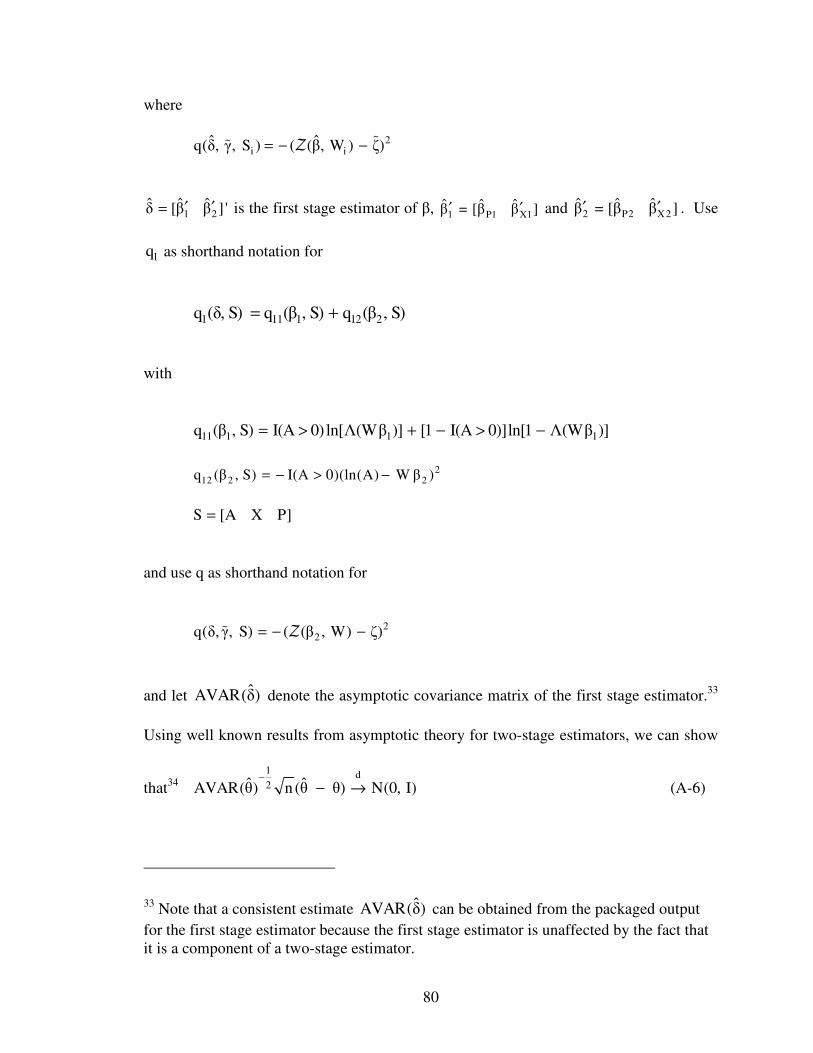
80

where

2i i

ˆ ˆq(δ, γ, S ) ( (β, W ) ζ)= − − Z

1 2ˆ ˆ ˆδ [β β ] '′ ′= is the first stage estimator of β, 1 P1 X1

ˆ ˆ ˆβ = [β β ]′ ′ and 2 P2 X2ˆ ˆ ˆβ = [β β ]′ ′ . Use

1q as shorthand notation for

1 11 1 12 2q (δ, S) q (β , S) q (β , S)= +

with

11 1 1 1q (β , S) I(A 0) ln[Λ(Wβ )] [1 I(A 0)]ln[1 Λ(Wβ )]= > + − > −

212 2 2q (β , S) I(A 0)(ln(A) W β )= − > −

S [A X P]=

and use q as shorthand notation for

22q(δ, γ, S) ( (β , W) ζ)= − − Z

and let ˆAVAR(δ) denote the asymptotic covariance matrix of the first stage estimator.33

Using well known results from asymptotic theory for two-stage estimators, we can show

that34

1 d2ˆ ˆAVAR(θ) n (θ θ) N(0, I)

−

− → (A-6)

33 Note that a consistent estimate ˆAVAR(δ) can be obtained from the packaged output

for the first stage estimator because the first stage estimator is unaffected by the fact that it is a component of a two-stage estimator.

81

where ˆˆ ˆθ = [δ γ]′ ′ , ˆplim(θ) = θ

11 12

12 22

D D

D DˆAVAR(θ)

= ′

(A-7)

11ˆAVAD R(δ)= (A-8)

2K×2K

[ ]12 δδ 1 δ 1 γ γγ

11E ED q q ' q E q

−−= ∇ ∇ ∇ ∇

[ ] [ ] [ ]δδ 1 δ 1 δ 1 δδ 1 γ

1

γ

1

δ

1

γE q q ' q q q qE E E E−− −

∇ ∇′ − ∇ ∇ ∇ ∇ (A-9)

and

22 γγ γδ γ

1

δˆˆAVAR (γ) E E AVD q q qAR(β)E '

− = = ∇ ∇ ∇

[ ]γ δ 1 δδ 1 γδ

1q q qE E E q

−∇ ∇

′ − ∇ ∇

[ ]γδ δδ 1 δ

1

γ γγ

1

1q qE E E ' Eq q q−−

∇ ∇ ∇ ∇ − ∇

21

γγ γγ

1

γE E qEq q− −

+ ∇ ∇ ∇ (A-10)

Fortunately, (A-9) and (A-10) can be simplified in a number of ways. First note that we

can write

γ δ 1 γ δ 1q q qE[ W]E |E q =∇ ∇ ∇ ∇

but

34Discussions of asymptotic theory for two-stage optimization estimators can be found in Newey & McFadden (1994), White (1994, Chapter 6), and Wooldridge (2010, Chapter 12).

82

δ 1 δ 11 δ 12q = q q∇ ∇ +∇

with

1δ 11 βq [ ln f (I(A 0) | W) 0 0]∇ = ∇ >

( )2δ 12q 0 2 ln(A)I(A 0) W β W 0= −>∇

where

I(A 0) [1 I(A 0)]1 1Λ(W β ) [1 Λ(W β )f (I( | W ]A 0) ) > − >= −> .

Therefore

( )11 β 2δE[ q | W] E[ ln f (I(A 0) | W)] 2E ln(A)I(A 0) Wβ | W W ∇ = ∇ > − >

= [ 0 0]

because 1β

E[ ln f (I(A 0) | W )] 0∇ > = [see (13.20) on p. 477 of Wooldridge (2010)] and,

( )2E ln(A)I( 0 0A ) W β | W− = > by design. Finally, then we get

γ δ 1E 0q q∇ = ∇

so

[ ] [ ] [ ]12 δδ 1 δ 1 δ 1 δδ 1 γδ γγ

11 1E E E ED q q ' q q q qE

−− − ′ − = ∇ ∇ ∇ ∇ ∇ ∇ (A-11)

2K×2K 2K×2K 2K×2K 2K×1 1×1 and

22 γγ γδ γδ γγ

1 1ˆˆAVAR(γ) E E AVAR(β) E 'ED q q q q− −

= ∇ ∇ ∇ = ∇

1×1 1×2K 2K×2K 2K×1 1×1

21

γγ γγ

1

γE E qEq q− −

+ ∇ ∇ ∇ . (A-12)

1×1 1×1 1×1

83

so

11 1

(2K 1) (2K

2

12 21) 2

D D

2K 2K 2K 1

D D

1 2K

ˆAVAR(

1 1

θ)+ × +

× × = ′

× ×

.

Let’s consider each of the individual components of (A-11) and (A-12) in turn.

δ1

δ 1qE[ ]−−−−∇∇∇∇

2K×2K

Written out explicitly we have

1 1

2 2

1β β 11

ββ 1 1β 12

1

β

E[ q ] 0q ]

0 E[

[E

q ]−

−

− ∇ ∇ = ∇

. (A-13)

Now

1 1

11 1β β 1E ˆAV[ ] )q AR(β− = −∇ (A-14)

= the negative of the asymptotic covariance matrix for first

stage, first part, logit estimation in the two-stage estimation

protocol for θ. We get an estimate of this directly from the Stata

output.

A consistent estimator of 1 1β β 11

1E[ q ]−∇ is

1 1

1β 1 1β 1

ˆ ˆnAVAR *(βE q ] )[ − = −∇ (A-15)

where 1ˆAVAR * (β ) is the estimated variance-covariance matrix output by the Stata logit

procedure. Also

2β 12 2I(A 0) Aq 2 )ln( β )W( W> −∇ =

84

and

2 2β β 12q 2 I(A 0)W W′>∇ = − .

Therefore

[ ]2 2β β 12E[ q ] I( )2E A 0 W W∇ = − ′> .

A consistent estimator of 2 2

1β β 12E[ q ]−∇ is

2 2 i

1n

1β β 12 1

i 1i iE[ q ] n 2 I(A 0)W W

−−

=

∑ ′>

∇ = − (A-17)

where 1n is the size of the subsample for whom I(A 0) 1> = , so

1 1

2 2

β β 11

δδ 1 ββ 1 1β

1

1

β

1

12

[ qEˆ ˆE[ E[

E

] 0q ] q ]

0 [ q ]−

−

− − ∇ ∇ = ∇ = ∇

. (A-18)

δ 1 δ 1q ' qE ∇ ∇∇ ∇∇ ∇∇ ∇

2K×2K Written out explicitly we have

1 1 1 2

2 1 2 2

β 11 β 11 β 11 β 12

β 1 β 1β 12 β 11 β 12 β 12

E[ q ' q ] E[ q ' q ]q ' q

E[ q ' q ] E[ q 'E

q ] =

∇ ∇ ∇ ∇ ∇ ∇

∇ ∇ ∇ ∇

. (A-19)

Because the first stage, first part, estimator of 1β is MLE we can write

1 1 1 1β 11 β 11 β β 11

1

1E[ q ' q ] E[ q ˆA (] VAR β )−

∇ = ∇ = ∇ −

= the inverse of the asymptotic covariance matrix for first stage,

85

first part, logit estimation in the two-stage estimation

protocol for θ. We get an estimate of this directly from the Stata

output.

A consistent estimator of 1 1β 11 β 11E[ q ' q ]∇ ∇ is

1 1β 11 β 1

1

1 1

1 ˆAVARE[ q ' *(β )n

q ]−

=

∇ ∇ (A-20)

where 1ˆAVAR * (β ) is the estimated variance-covariance matrix output by the Stata logit

procedure. The remaining block elements follow from

[ ]1 1β 11 β 1 1q ln f (I(A 0) | W) I(A 0) W β )] [1[1 Λ( I(A 0)] W β ) WΛ(−∇ = ∇ > = > − − >

(A-21)

( )2 2β 12q 2 ln(A |I A(A 0) W β W0)∇ = > −> . (A-22)

where the formulation of 1β 11q∇ comes from equation (16.4.8) on p. 350 of Fomby et al.

(1984) and Λ( ) denotes the logistic cdf. The remaining required consistent matrix

estimators are

1 2 1 2

n

β 11 β 12 β 11i β 12ii 11

1ˆ ˆ ˆE[ q ' q ] q ' qn =

∑∇ ∇ = ∇ ∇ (A-23)

2 2 2 2

n

β 12 β 12 β 12i β 12ii 11

1ˆ ˆ ˆE[ q ' q ] q ' qn =

∑∇ ∇ = ∇ ∇ (A-24)

where

1β 11i i i 1 1i i i

ˆ ˆW β )]q I(A 0)[1 Λ( I(A 0)]Λ([1 W β ) W∇ = > − > − − (A-25)

86

and

( )2β 12i i i i i i2q 2 A ln(A | A 0 ˆI( 0) W β) W> −>∇ = (A-26)

so

[ ] 1 1 1 2

2 1 2 2

β 11 β 11 β 11 β 12

δ 1 δ 1 β 1 β 1

β 12 β 11 β 12 β 12

ˆ ˆE Eˆ ˆE E

ˆ

[ q ' q ] [ q ' q ]q ' q q ' q

[ q ˆE ' q ] [ q ' q ]E

∇ ∇ ∇ ∇ ∇ ∇ ∇ ∇ ∇ ∇

= =∇

∇

.(A-27)

γδqE ∇∇∇∇

1×2K Written out explicitly we have

( )γ ζ cq = q 2 (β, S) ζ=∇ ∇ −Z (A-28)

and

1γδ ζβE[ q] = E[ q] 0 ∇ ∇

1β

= 2 E[ ] 0 ∇ Z (A-29)

where

1 1β λ(Wβ ) W∇ =Z . (A-30)

The requisite consistent matrix estimator is

1 1

n

β β ii 1

E[ ] ==∑∇ ∇Z Z (A-31)

where

1β i ii 1

ˆλ(W β W= )∇ Z (A-32)

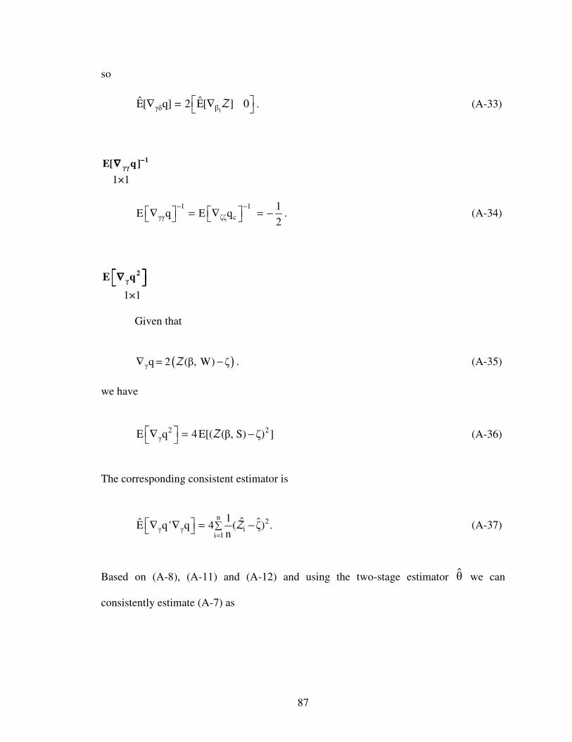
87

so

1γδ β

ˆ ˆE[ q] = 2 E[ ] 0 ∇ ∇ Z . (A-33)

γγ1E[ q]−−−−∇∇∇∇

1×1

γγ ζζ

1 1

cq q1

E E2

− − ∇ ∇ = = − . (A-34)

2γE q∇∇∇∇

1×1

Given that

( )γ 2 (β, W ζq )∇ = −Z . (A-35)

we have

2 2γE 4E[( (β, Sq ) ζ) ] = − ∇ Z (A-36)

The corresponding consistent estimator is

n

2

1γ iγ

i

1 ˆ ˆE 4 ( ζ) .n

q ' q=∑∇ − ∇ = Z (A-37)

Based on (A-8), (A-11) and (A-12) and using the two-stage estimator θ we can

consistently estimate (A-7) as

88

11 12

12 22

ˆ ˆD D

ˆ ˆD D

ˆAVAR(θ)

= ′

where

1

2

11

1

ˆnAVAR * 0(β )ˆ ˆAVAR(δ) AVAR(β)ˆn AVA

DR *(β )0

=

=

=

[ ]12 γγ δ 1 δ 1 γγ γδ γ

1 1

γ

1ˆ ˆ ˆ ˆ ˆE E E E ED q q ' q q q q− − −′ = ∇ ∇ ∇ ∇ ∇ ∇ −

22 γγ γδ

1 1

γδ γγˆˆ ˆ ˆ ˆˆAVAR(γ) E E AVAR(β) E 'D q Eq q q

− − = ∇ ∇ ∇ = ∇

2γ γγ

1

γ γ

1q q qˆ ˆ ˆE E E

− − + ∇ ∇ ∇

and using well known results from asymptotic theory for two-stage estimators, we can

show that35

1 11d

21 2 2

ˆn(β β )

ˆ ˆˆAVAR(θ) n (β β ) N(0, I)

ˆn (ζ ζ)

−

−

− →

−

. (A-38)

************************************************************************

ASIDE:

35Discussions of asymptotic theory for two-stage optimization estimators can be found in Newey & McFadden (1994), White (1994, Chapter 6), and Wooldridge (2010, Chapter 12).

89

Notice that the “ n blow up” is a bit tricky here. It implements n for 1β and ζ ; but

uses 1n for 2β . We had to do this because we had to use the correct sample size (viz.,

1n ) for a number of the components of AVAR(θ) [viz., those that pertained to the

estimation of 2β ]; in particular (A-17), (A-23) and (A-24). For this reason we had to be

explicit about the denominators in all of the averages for the components of AVAR(θ) .

This meant that in the construction of the requisite asymptotic t-stats we had to explicitly

include the “blow-up” in the numerator (i.e., we had to multiply by the square-root of the

appropriate sample size). I refer to this as “tricky” because one typically does not have to

do this. In the usual asymptotic t-stat construction the denominators of the averages (“n”)

need not be included in the construction of the asymptotic covariance matrix because it

typically manifests as a multiplicative factor and, after pulling the diagonal and taking the

square root to get the standard errors, this multiplicative n cancels with the “blow-up”

factor in the numerator. For example, the asymptotic t-stat of the OLS estimator is

( ) ( )

k k k k k k k k

1 1 12 22 kk kk

kk

ˆ ˆ ˆ ˆn (ρ ρ ) n (ρ ρ ) n (ρ ρ ) (ρ ρ )

ˆAVAR(ρ) ˆ ˆn σ σ1σ

n

− − −

− − − −= = =

′ ′ ′

XX XXXX

where

n is the sample size

kρ is the coefficient of the kth regressor in the linear regression

kρ is its OLS estimator

2σ is the regression error variance estimator

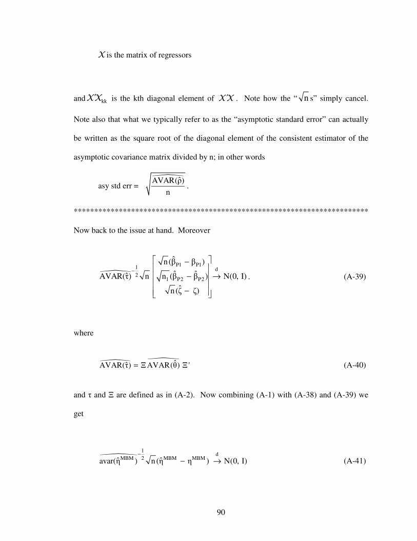
90

X is the matrix of regressors

and kk′XX is the kth diagonal element of ′XX . Note how the “ n s” simply cancel.

Note also that what we typically refer to as the “asymptotic standard error” can actually

be written as the square root of the diagonal element of the consistent estimator of the

asymptotic covariance matrix divided by n; in other words

asy std err = AVAR(ρ)

n.

************************************************************************

Now back to the issue at hand. Moreover

P1 P11 d

21 P2 P2

ˆn(β β )

ˆ ˆˆAVAR(τ) n n (β β ) N(0, I)

ˆn (ζ ζ)

−

−

− →

−

. (A-39)

where

ˆAVAR(τ) ΞAVAR(θ) Ξ '= (A-40)

and τ and Ξ are defined as in (A-2). Now combining (A-1) with (A-38) and (A-39) we

get

1d

MBM MBM MBM2ˆ ˆavar(η ) n (η η ) N(0, I)−

− → (A-41)

91

where

MBMˆ ˆ ˆ ˆavar(η ) c(τ) AVAR(τ) c(τ) '=

and

P1c(τ) [(1 ζ) 1 β ]= − − .

92

Appendix B:

Asymptotic Distribution (and Standard Error) of POη in Eqn (2-7)

We may write POη as

PO κη

ν=

where

n

ii 1

1 ˆκ (β, W )n=

∑= K

n

ii 1

1 ˆν = (β, W )n=

∑ V

1 2 P1 1 2 P2(β, W) λ(Wβ )exp(Wβ )β Λ(Wβ )exp(Wβ )β+=K

1 2(β, W) Λ(W β ) exp(W β )=V

1 2ˆ ˆ ˆβ [β β ]'′ ′= (with 1 P1 X1

ˆ ˆ ˆβ = [β β ]′ ′ and 2 P2 X2ˆ ˆ ˆβ = [β β ]′ ′ ) is the consistent

estimate of the parameter vector 1 2β [β β ]'′ ′= (with 1 P1 X1β = [β β ]′ ′ and

2 P2 X2β = [β β ])′ ′ ) [the parameters of equations (2-1) and (2-2)] obtained

via the two-part protocol culminating in (2-3)

and

i i iW [P X ]= denotes the observation on W [P X]= for the ith individual in

the sample (i = 1, ..., n). Let ˆ ˆγ = [κ ν]′ and γ = [κ ν]′ , where ˆplim[γ] = γ .

If we could show that

93

1 d2ˆ ˆAVAR(γ) n (γ γ) N(0, I)

−

− →

where the formulation of ˆAVAR(γ) is known, then we could apply the δ-method to

obtain the asymptotic variance of POη as

POˆ ˆavar(η ) c(γ) AVAR(γ) c(γ) '=

where 2c(τ) [1/ ν κ / ν ]= − . Moreover, if we have a consistent estimator for ˆAVAR(γ)

, say AVAR(γ) [i.e. ˆp lim AVAR(γ) AVAR(γ) =

], then we could consistently

estimate POˆavar(η ) as

POˆ ˆ ˆ ˆavar(η ) c(γ) AVAR(γ) c(γ) '= . (B-1)

We focus, therefore, on finding the asymptotic distribution of γ and, in particular, the

formulation of its asymptotic covariance matrix.

First, let θ = [δ γ ]′ ′ ′ where 1 2δ [β β ]'′ ′= , γ [κ ν]′ = (recall, 1 P1 X1β = [β β ]′ ′

and 2 P2 X2β = [β β ]′ ′ ), and note that γ can be viewed as the second stage estimator in the

following two-stage protocol

First Stage

Consistently estimate δ via the following optimization estimator

n

1 ii 1

δ

q (δ, S )δ = arg max

n=∑

(B-2)

94

where

1 i 11 1 i 12 2 iq (δ, S ) q (β , S ) q (β , S )= +

11 1 i i i 1 i i 1q (β , S ) I(A 0) ln[Λ(W β )] [1 I(A 0)] ln[1 Λ(W β )]= > + − > −

212 2 i i i i 2q (β , S ) I(A 0)(ln(A ) W β )= − > −

i i i iS [A X P ]=

1 22δ [β β ]'′ ′= , 1 P1 X1β = [β β ]′ ′ and 2 P2 X2β = [β β ]′ ′ and 1 22ˆ ˆ ˆδ [β β ]'′ ′=

Second Stage

Consistently estimate γ via the following optimization estimator

n

ii 1

γ

ˆq(δ, γ, S )γ = arg max

n=∑

(B-3)

where

i a i b iˆ ˆ ˆq(δ, γ, S ) q (δ, κ, S ) q (δ, ν, S )= +

2a i i

ˆ ˆq (δ, κ, S ) ( (β, W ) κ)= − − K

2b i i

ˆ ˆq (δ, ν, S ) ( (β, W ) ν)= − − V

1 2ˆ ˆ ˆδ [β β ] '′ ′= is the first stage estimator of δ, 1 P1 X1

ˆ ˆ ˆβ = [β β ]′ ′ and 2 P2 X2ˆ ˆ ˆβ = [β β ]′ ′ . Use

1q as shorthand notation for

1 11 1 12 2q (δ, S) q (β , S) q (β , S)= +

with

95

11 1 1 1q (β , S) I(A 0) ln[Λ(Wβ )] [1 I(A 0)]ln[1 Λ(Wβ )]= > + − > −

212 2 2q (β , S) I(A 0)(ln(A) W β )= − > −

S [A X P]=

and use q as shorthand notation for

a bq(δ, γ, S) q (δ, κ, S) q (δ, ν, S)= +

with

2aq (δ, κ, S) ( (β, W) κ)= − −K

2bq (δ, ν, S) ( (β, W) ν)= − −V

and let ˆAVAR(δ) denote the asymptotic covariance matrix of the first stage estimator.36

Using well known results from asymptotic theory for two-stage estimators, we can show

that37

1 d2ˆ ˆAVAR(γ) n (γ γ) N(0, I)

−

− → (B-4)

where, ˆplim(γ) = γ

γ γδ γδ

1

γq q ˆˆAVAR (γ) E E AVAR (β)E q '−

∇ ∇ ∇ =

36 Note that a consistent estimate ˆAVAR(δ) can be obtained from the packaged output

for the first stage estimator because the first stage estimator is unaffected by the fact that it is a component of a two-stage estimator. 37Discussions of asymptotic theory for two-stage optimization estimators can be found in Newey & McFadden (1994), White (1994, Chapter 6), and Wooldridge (2010, Chapter 12).

96

[ ]γ δ 1 δδ 1 γδ

1q ' q qE E E q

−∇ ∇

′ − ∇ ∇

[ ]γδ δδ 1 γ δ 1 γ

1

γ

1q q q ' q qE E E ' E

−− − ∇ ∇∇ ∇ ∇

1 1

γγ γ γ γγq q ' q qE E E− −

∇ ∇ ∇ + ∇ (B-5)

Fortunately, (B-5) can be simplified in a number of ways. Note that we can write

γ δ 1 γ δ 1q ' q q 'E E[ q | W]E∇ ∇ ∇ ∇ =

but

δ 1 δ 11 δ 12q = q q∇ ∇ +∇

with

1δ 11 βq [ ln f (I(A 0) | W) 0 0]∇ = ∇ >

( )2δ 12q 0 2 ln(A)I(A 0) W β W 0= −>∇

where

I(A 0) [1 I(A 0)]1 1Λ(W β ) [1 Λ(W β )f (I( | W ]A 0) ) > − >= −> .

Therefore

( )11 β 2δE[ q | W] E[ ln f (I(A 0) | W)] 2E ln(A)I(A 0) Wβ | W W ∇ = ∇ > − >

= [ 0 0]

because

1βE[ ln f (I(A 0) | W )] 0∇ > = [see (13.20) on p. 477 of Wooldridge (2010)] and,

( )2E ln(A)I( 0 0A ) W β | W− = > by design. Finally, then we get

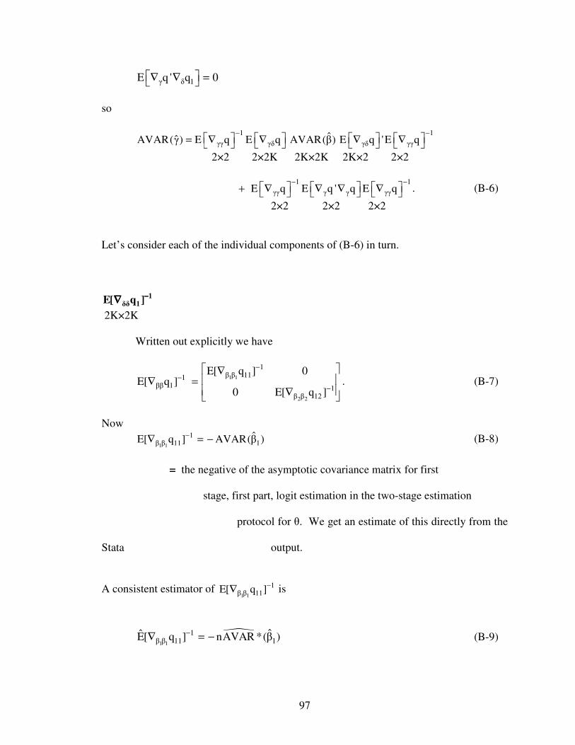
97

γ δ 1q ' qE 0 = ∇ ∇

so

γγ γδ γδ γγ

1 1ˆˆAVAR(γ) E E AVAR(β) E 'Eq q q q− −

∇ ∇ ∇ ∇ =

2×2 2×2K 2K×2K 2K×2 2×2

1 1

γγ γ γ γγq q ' q qE E E− −

∇ ∇ ∇ + ∇ . (B-6)

2×2 2×2 2×2 Let’s consider each of the individual components of (B-6) in turn.

δ1

δ 1qE[ ]−−−−∇∇∇∇

2K×2K

Written out explicitly we have

1 1

2 2

1β β 11

ββ 1 1β 12

1

β

E[ q ] 0q ]

0 E[

[E

q ]−

−

− ∇ ∇ = ∇

. (B-7)

Now

1 1

11 1β β 1E ˆAV[ ] )q AR(β− = −∇ (B-8)

= the negative of the asymptotic covariance matrix for first

stage, first part, logit estimation in the two-stage estimation

protocol for θ. We get an estimate of this directly from the

Stata output.

A consistent estimator of 1 1β β 11

1E[ q ]−∇ is

1 1

1β 1 1β 1

ˆ ˆnAVAR *(βE q ] )[ − = −∇ (B-9)

98

where 1ˆAVAR * (β ) is the estimated variance-covariance matrix output by the Stata logit

procedure. Also

2β 12 2I(A 0) Aq 2 )ln( β )W( W> −∇ =

and

2 2β β 12q 2 I(A 0)W W′>∇ = − .

Therefore

[ ]2 2β β 12E[ q ] I( )2E A 0 W W∇ = − ′> . (B-10)

A consistent estimator of 2 2

1β β 12E[ q ]−∇ is

2 2 i

1n

1β β 12 1

i 1i iE[ q ] n 2 I(A 0)W W

−−

=∑ ′>

∇ = −

(B-11)

where 1n is the size of the subsample for whom I(A 0) 1> = , so

1 1

2 2

β β 11

δδ 1 ββ 1 1β

1

1

β

1

12

[ qEˆ ˆE[ E[

E

] 0q ] q ]

0 [ q ]−

−

− − ∇ ∇ = ∇ = ∇

. (B-12)

δ 1 δ 1q ' qE ∇ ∇∇ ∇∇ ∇∇ ∇

2K×2K Written out explicitly we have

1 1 1 2

2 1 2 2

β 11 β 11 β 11 β 12

β 1 β 1β 12 β 11 β 12 β 12

E[ q ' q ] E[ q ' q ]q ' q

E[ q ' q ] E[ q 'E

q ] =

∇ ∇ ∇ ∇ ∇ ∇

∇ ∇ ∇ ∇

. (B-13)

99

Because the first stage, first part, estimator of 1β is MLE we can write

1 1 1 1β 11 β 11 β β 11

1

1E[ q ' q ] E[ q ˆA (] VAR β )−

∇ = ∇ = ∇ −

= the inverse of the asymptotic covariance matrix for first stage,

first part, logit estimation in the two-stage estimation

protocol for θ. We get an estimate of this directly from the

Stata output.

A consistent estimator of 1 1β 11 β 11E[ q ' q ]∇ ∇ is

1 1β 11 β 1

1

1 1

1 ˆAVARE[ q ' *(β )n

q ]−

=

∇ ∇ (B-14)

where 1ˆAVAR * (β ) is the estimated variance-covariance matrix output by the Stata logit

procedure. The remainder of the block elements follow from

1 1β 11 βq ln f (I(A 0) | W)∇ = ∇ >

[ ]1 1Wβ )I( ] [1 Wβ )A 0)[1 Λ( I W(A 0)]Λ(− >−= > −

(B-15)

( )2 2β 12q 2 ln(A |I A(A 0) W β W0)∇ = > −> . (B-16)

where the formulation of 1β 11q∇ comes from equation (16.4.8) on p. 350 of Fomby et al.

(1984) and Λ( ) denotes the logistic cdf. The remaining required consistent matrix

estimators are:

100

1 2 1 2

n

β 11 β 12 β 11i β 12ii 11

1ˆ ˆ ˆE[ q ' q ] q ' qn =

∑∇ ∇ = ∇ ∇ (B-17)

2 2 2 2

n

β 12 β 12 β 12i β 12ii 11

1ˆ ˆ ˆE[ q ' q ] q ' qn =

∑∇ ∇ = ∇ ∇ (B-18)

where

1β 11i i i 1 1i i i

ˆ ˆW β )]q I(A 0)[1 Λ( I(A 0)]Λ([1 W β ) W∇ = > − > − − (B-19)

and

( )2β 12i i i i i i2q 2 A ln(A | A 0 ˆI( 0) W β) W> −>∇ = (B-20)

so

[ ] 1 1 1 2

2 1 2 2

β 11 β 11 β 11 β 12

δ 1 δ 1 β 1 β 1

β 12 β 11 β 12 β 12

ˆ ˆE Eˆ ˆE E

ˆ

[ q ' q ] [ q ' q ]q ' q q ' q

[ q ˆE ' q ] [ q ' q ]E

∇ ∇ ∇ ∇ ∇ ∇ ∇ ∇ ∇ ∇

= =∇

∇

.(B-21)

γδqE ∇∇∇∇

2×2K Written out explicitly we have

γ κ a ν bq = [( q 0) (0 q )]∇ ∇ + +∇

κ a ν b[ q q ] ∇ ∇=

( ) ( )2 (β, S) κ (β, S) ν = − − K V (B-22)

and

1 2

1 2

κβ a κβ a

γδ

νβ b νβ b

E[ q ] E[ q ]E[ q] =

E[ q ] E[ q ]

∇ ∇ ∇

∇ ∇

1 2

1 2

β β

β β

E[ ] E[ ]= 2

E[ ] E[ ]

∇ ∇

∇ ∇

K K

V V (B-23)

101

where

1 1 1 P1 1 2β λ(Wβ )[1 2Λ(Wβ )]β W λ(Wβ )[1 0 ... 0]exp(Wβ )− +∇ =K

1 2 P2λ(Wβ )exp(Wβ )β W+

[ ]1 2 1 P1 P2λ(Wβ ) exp(Wβ ) [1 2Λ(Wβ )]β + β W [1 0 ... 0]= − + (B-24)

2 1 2 P1 1 2 P 2β 2λ(Wβ ) exp(Wβ )β W+ Λ(Wβ )exp(Wβ )β W exp(Wβ )[1 0 ... 0]=∇ +K

[ ]2 1 P1 1 P2 1exp(Wβ ) λ(Wβ )β + Λ(Wβ )β W Λ(Wβ )[1 0 ... 0]= + . (B-25)

1 1β 2λ(W β ) exp(W β ) W∇ =V (B-26)

and

2 1β 2Λ(W β ) exp(W β ) W∇ =V . (B-27)

The following equalities were used in deriving the above results

aΛ(a) λ(a) Λ(a)[1 Λ(a)]∇ = = −

aλ(a) λ(a)[1 2Λ(a)]∇ = − .

The requisite consistent matrix estimators are

1 1

n

β β ii 1

E[ ] ==∑∇ ∇K K (B-28)

2 2

n

β β ii 1

E[ ] ==∑∇ ∇K K (B-29)

1 1

n

β β ii 1

E[ ] ==∑∇ ∇V V (B-30)

and

2 2

n

β β ii 1

E[ ] ==∑∇ ∇V V (B-31)

where

102

1 1 2 1 P1 P2β i i i ii

ˆ ˆ ˆ ˆ ˆλ(W β ) exp(W β ) [1 2Λ(W β )]β + β W [1 0 ... 0] = − + ∇ K (B-32)

2β i i i i ii 2 1 P1 1 P2 1

ˆ ˆ ˆ ˆ ˆ ˆexp(W β ) λ(W β )β + Λ(W β )β W Λ(W β )[1 0 ... 0]∇ = + K (B-33)

1 1 2β i i ii

ˆ ˆλ(W β ) exp(W β W= )∇ V (B-34)

and

1 1 2β i i ii

ˆ ˆΛ(W β ) exp(W β W= )∇ V . (B-35)

so

1 2

1 2

β β

γδ

β β

ˆ ˆE[ ] E[ ]E[ q] = 2

ˆ ˆE[ ] E[ ]

∇ ∇ ∇ ∇ ∇

K K

V V. (B-37)

γγ1E[ q]−−−−∇∇∇∇

2×2

[ ]

[ ]

1

κκ a

γγ

νν

1

b

1 E 0E

qq

q0 E

−−

−

∇∇

∇ =

(B-38)

because κν a νκ bq q 0∇ = ∇ = . Now

κκ a νν bq q 2∇ = ∇ = −

therefore

1

γγ

10

2E

10

q

2

−

−

=

∇−

. (B-39)

γ γq' qE ∇ ∇∇ ∇∇ ∇∇ ∇

103

2×2

Given that

( ) ( )γ 2 (β, W) κ (β, W) νq = − − ∇ K V . (B-40)

we have

γ 2γ

2E[( (β, S) κ) ] E[( (β, S) κ)( (β, S) ν)]E 4

E[( (β, S) κ)( (β, S) ν)] E[( (β, S) ν)' q

]q

− − − =

− − − ∇ ∇

K K V

K V V.

(B-41) The corresponding consistent estimator is

n n2

i i ii 1 i 1

n n2

i i ii

γ

1

γ

i 1

1 1 ˆˆ ˆˆ ˆ ˆ( κ) ( κ)( ν)n n

E 41 1ˆ ˆˆ ˆ ˆ ˆ( κ)( ν

q ' q

) ( ν)n n

= =

= =

∑ ∑

∑ ∑

− − −

= − − −

∇ ∇

K K V

K V V

. (B-42)

Based on the above results, we can consistently estimate (B-5) as

γγ γδ δ γγ

1 1

γˆˆ ˆ ˆ ˆˆAVAR(γ) E E Aq q qVAR(β) E q'E

− − ∇ = ∇ ∇ ∇

γγ γ γ γγ

1 1q q ' q qˆ ˆ ˆE E E

− −∇ ∇ ∇ + ∇

and using well known results from asymptotic theory for two-stage estimators, we can

show that38

38Discussions of asymptotic theory for two-stage optimization estimators can be found in Newey & McFadden (1994), White (1994, Chapter 6), and Wooldridge (2010, Chapter 12).

104

1 d2ˆ ˆAVAR(γ) n (γ γ) N(0, I)

−

− → . (B-43)

Combining (B-43) with (B-1) we also have that

1d

PO PO PO2ˆ ˆavar(η ) n (η η ) N(0, I)−

− → (B-44)

where POˆavar(η ) is given in (B-1).

105

Appendix C.

Bias from Using MBMη Instead of POη in a Two-Part Model

If we define

1 2ν E[Λ(Wβ )exp(Wβ )]≡

1ζ E[Λ(Wβ )]≡

and

21 2ω E[Λ(Wβ ) exp(Wβ )]≡

we can write the bias from using the MBM approach vs. the correct PO method as the

following rendition of the difference between (2-5) and (2-7)

MBM PO P1 1 2 P2P1 P2

β E[λ(Wβ ) exp(Wβ )] β νη η [ (1 ζ)β β ]

ν

+ − = − + −

[P1 1 1 2 P2

P1 P2

β E Λ(Wβ )[1 Λ(Wβ )]exp(Wβ ) β ν[ (1 ζ)β β ]

ν

− += − + −

2

P1 P1 1 2 P2P1 P2

β ν β E[Λ(Wβ ) exp(Wβ )] β ν[ (1 ζ)β β ]

ν

− += − + −

P1 P1 P2 P1 P1 P2

ωβ ζβ β β β β

ν= − + − + −

P1 P1

ω ˆβ β ζν

= −

P1

ωβ ζ

ν

= −

.

106

Appendix D.

Asymptotic Distribution (and Standard Error) of MBM POˆ ˆη η−

In Appendix C we showed that

MBM POP1

ωη η β ζ

ν

− = −

where

1 2ν E[Λ(Wβ )exp(Wβ )]≡

1ζ E[Λ(Wβ )]≡

and

21 2ω E[Λ(Wβ ) exp(Wβ )]≡ .

Using the corresponding consistent estimators for ω, ν and ζ we can write

MBM POP1

ωˆ ˆˆ ˆη η β ζν

− = −

where

n

ii 1

1 ˆω Ω(β, W )n=

∑=

n

ii 1

1 ˆν = (β, W )n=

∑ V

n

1 ii 1

1ˆ ˆζ = (β , W )n=

∑ Z

21 2Ω(β, W) Λ(Wβ ) exp(Wβ )=

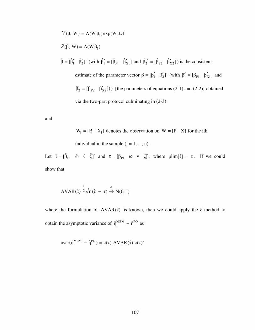
107

1 2(β, W) Λ(W β ) exp(W β )=V

1(β, W) Λ(Wβ )=Z

1 2ˆ ˆ ˆβ [β β ]'′ ′= (with 1 P1 X1

ˆ ˆ ˆβ = [β β ]′ ′ and 2 P2 X2ˆ ˆ ˆβ = [β β ]′ ′ ) is the consistent

estimate of the parameter vector 1 2β [β β ]'′ ′= (with 1 P1 X1β = [β β ]′ ′ and

2 P2 X2β = [β β ])′ ′ ) [the parameters of equations (2-1) and (2-2)] obtained

via the two-part protocol culminating in (2-3)

and

i i iW [P X ]= denotes the observation on W [P X]= for the ith

individual in the sample (i = 1, ..., n).

Let P1ˆ ˆˆ ˆτ = [β ω ν ζ]′ and P1τ = [β ω ν ζ]′ , where ˆplim[τ] = τ . If we could

show that

1 d2ˆ ˆAVAR(τ) n (τ τ) N(0, I)

−

− →

where the formulation of ˆAVAR(τ) is known, then we could apply the δ-method to

obtain the asymptotic variance of MBM POˆ ˆη η− as

MBM POˆ ˆ ˆavar(η η ) c(τ) AVAR(τ) c(τ) '− =

108

where 2P1

ωc(τ) ζ 1/ ν ω / ν β

ν

= − − −

. Moreover, if we have a consistent

estimator for ˆAVAR(τ) , say AVAR(τ) [i.e. ˆp lim AVAR(τ) AVAR(τ) =

], then we

could consistently estimate MBM POˆ ˆavar(η η )− as

MBM POˆ ˆ ˆ ˆ ˆavar(η η ) c(τ) AVAR(τ) c(τ) '− = . (D-1)

We focus, therefore, on finding the asymptotic distribution of τ and, in particular, the

formulation of its asymptotic covariance matrix.

First note that we can write τ as

τ Ξ θ= (D-2)

where θ = [δ γ ]′ ′ ′ , 1 2δ [β β ]'′ ′= , γ [ω ν ζ]′ = (recall, 1 P1 X1β = [β β ]′ ′ and

2 P2 X2β = [β β ]′ ′ )

P1β

3,2K 3

Ξ

0 I

= − − − − − − − −

a is the unit row vector with the value “1” in the element position corresponding to the

element position of a in the vector θ, b,c0 is the matrix of zeros whose row and column

dimensions are b and c, respectively, dI is the identity matrix of order d, and K is the

109

column dimension of W. For future reference, let’s set the following vector/matrix

dimensions:

1β is K×1

2β is K×1

W is 1×K

τ is 4×1

c(τ) is 1×4

δ is 2K×1

γ is 3×1

θ is (2K+3)×1

Ξ is 4×(2K+3)

P1β is 1×(2K+3)

Clearly then

ˆˆAVAR(τ) Ξ AVAR(θ) Ξ′= (D-3)

where θ is the estimator of θ obtained from the following two-stage protocol.

First Stage

Consistently estimate β via the following optimization estimator

n

1 ii 1

δ

q (δ, S )δ = arg max

n=∑

(D-4)

110

where

1 i 11 1 i 12 2 iq (δ, S ) q (β , S ) q (β , S )= +

11 1 i i i 1 i i 1q (β , S ) I(A 0) ln[Λ(W β )] [1 I(A 0)] ln[1 Λ(W β )]= > + − > −

212 2 i i i i 2q (β , S ) I(A 0)(ln(A ) W β )= − > −

i i i iS [A X P ]=

1 22δ [β β ]'′ ′= , 1 P1 X1β = [β β ]′ ′ and 2 P2 X2β = [β β ]′ ′ and 1 22ˆ ˆ ˆδ [β β ]'′ ′=

Second Stage

Consistently estimate γ via the following optimization estimator

n

ii 1

γ

ˆq(δ, γ, S )γ = arg max

n=∑

(D-5)

where

i a i b i c iˆ ˆ ˆ ˆq(δ, γ, S ) q (δ, ω, S ) q (δ, ν, S ) q (δ, ζ, S )= + +

2a i i

ˆ ˆq (δ, ω, S ) (Ω(β, W ) ω)= − −

2b i i

ˆ ˆq (δ, ν, S ) ( (β, W ) ν)= − − V

2c i i

ˆ ˆq (δ, ζ, S ) ( (β, W ) ζ)= − − Z

1 2ˆ ˆ ˆδ [β β ] '′ ′= is the first stage estimator of β, 1 P1 X1

ˆ ˆ ˆβ = [β β ]′ ′ and 2 P2 X2ˆ ˆ ˆβ = [β β ]′ ′ . Use

1q as shorthand notation for

1 11 1 12 2q (δ, S) q (β , S) q (β , S)= +

111

with

11 1 1 1q (β , S) I(A 0) ln[Λ(Wβ )] [1 I(A 0)]ln[1 Λ(Wβ )]= > + − > −

212 2 2q (β , S) I(A 0)(ln(A) W β )= − > −

S [A X P]=

and use q as shorthand notation for

a b cq(δ,γ, S) q (δ, ω, S) q (δ, ν, S) q (δ, ζ, S)= + +

with

2aq (δ, ω, S) (Ω(β, W) ω)= − −

2bq (δ, ν, S) ( (β, W) ν)= − −V

2c 2q (δ, ζ, S) ( (β , W) ζ)= − −Z

and let ˆAVAR(δ) denote the asymptotic covariance matrix of the first stage estimator.39

Using well known results from asymptotic theory for two-stage estimators, we can show

that40

1 d2ˆ ˆAVAR(θ) n (θ θ) N(0, I)

−

− → (D-6)

where ˆˆ ˆθ = [δ γ ]′ ′ ′ , ˆplim(θ) = θ

39 Note that a consistent estimate ˆAVAR(δ) can be obtained from the packaged output

for the first stage estimator because the first stage estimator is unaffected by the fact that it is a component of a two-stage estimator. 40Discussions of asymptotic theory for two-stage optimization estimators can be found in Newey & McFadden (1994), White (1994, Chapter 6), and Wooldridge (2010, Chapter 12).

112

11 12

12 22

D D

D DˆAVAR(θ)

= ′

(D-7)

11ˆAVAD R(δ)= (D-8)

2K×2K

[ ]12 δδ 1 δ 1 γ γγ

11E ED q q ' q E q

−−= ∇ ∇ ∇ ∇

[ ] [ ] [ ]δδ 1 δ 1 δ 1 δδ 1 γ

1

γ

1

δ

1

γE q q ' q q q qE E E E−− −

∇ ∇′ − ∇ ∇ ∇ ∇ (D-9)

22 γγ γδ γ

1

δˆˆAVAR (γ) E E AVD q q qAR (β)E '

− = = ∇ ∇ ∇

[ ]γ δ 1 δδ 1 γδ

1q ' q qE E E q

−∇ ∇

′ − ∇ ∇

[ ]γδ δδ 1 γ δ 1 γ

1

γ

1q q q ' q qE E E ' E

−− − ∇ ∇∇ ∇ ∇

1 1

γγ γ γ γγq q ' q qE E E− −

∇ ∇ ∇ + ∇ . (D-10)

Fortunately, (D-9) and (D-10) can be simplified in a number of ways. First note that we

can write

γ δ 1 γ δ 1q ' q q 'E E[ q | W]E∇ ∇ ∇ ∇ =

but

δ 1 δ 11 δ 12q = q q∇ ∇ +∇

with

1δ 11 βq [ ln f (I(A 0) | W) 0 0]∇ = ∇ >

[ ]δ 2 21 I(A 0)q 0 2 ln(A( W β) )W 0∇ = −>

where

113

I(A 0) [1 I(A 0)]1 1Λ(W β ) [1 Λ(W β )f (I( | W ]A 0) ) > − >= −> .

Therefore

[ ]11 β 2δE[ q | W] E[ ln f (I(A 0) | W)] 2E ln(AI(A 0)( Wβ ) | W) W ∇ = ∇ > − >

= [ 0 0]

because 1β

E[ ln f (I(A 0) | W )] 0∇ > = [see (13.20) on p. 477 of Wooldridge (2010)] and,

[ ]2E ln(AI(A 0)( W β )) W 0|> − = by design. Finally, then we get

γ δ 1q ' qE 0 = ∇ ∇

so

[ ] [ ] [ ]12 δδ 1 δ 1 δ 1 δδ 1 γδ γγ

11 1E E E ED q q ' q q q qE

−− − ′ − = ∇ ∇ ∇ ∇ ∇ ∇ (D-11)

2K×2K 2K×2K 2K×2K 2K×3 3×3 2K×3 and

22 γγ γδ γδ γγ

1 1ˆˆAVAR(γ) E E AVAR(β) E 'ED q q q q− −

= ∇ ∇ ∇ = ∇

3×3 3×2K 2K×2K 2K×3 3×3

1 1

γγ γ γ γγq q ' q qE E E− −

∇ ∇ ∇ + ∇ . (D-12)

3×3 3×3 3×3 3×3 so

11 1

(2K 3) (2K

2

12 23) 2

D D

2K 2K 2K 3

D D

3 2K

ˆAVAR(

3 3

θ)+ × +

× × = ′

× ×

.

Let’s consider each of the individual components of (D-6) and (D-7) in turn.

114

δ1

δ 1qE[ ]−−−−∇∇∇∇

2K×2K

Written out explicitly we have

1 1

2 2

1β β 11

ββ 1 1β 12

1

β

E[ q ] 0q ]

0 E[

[E

q ]−

−

− ∇ ∇ = ∇

. (D-13)

Now

1 1

11 1β β 1E ˆAV[ ] )q AR(β− = −∇ (D-14)

= the negative of the asymptotic covariance matrix for first

stage, first part, logit estimation in the two-stage estimation

protocol for θ. We get an estimate of this directly from the Stata

output.

A consistent estimator of 1 1β β 11

1E[ q ]−∇ is

1 1

1β 1 1β 1

ˆ ˆnAVAR *(βE q ] )[ − = −∇ (D-15)

where 1ˆAVAR * (β ) is the estimated variance-covariance matrix output by the Stata logit

procedure. Also

2β 1 22 I(A 0)q 2 ln(A( W W) β )∇ = −>

and

2 2β β 12q 2 I(A 0)W W′>∇ = − .

Therefore

115

[ ]2 2β β 12E[ q ] I( )2E A 0 W W∇ = − ′> . (D-16)

A consistent estimator of 2 2

1β β 12E[ q ]−∇ is

2 2

1n

1β β 12

i1i i

1iI(A

1E[ q ] 0)W W2

n

−

−

=

∑

∇ −

>=

′

i

1n

11

ii

iI(A 0)W Wn 2−

=∑

= −

′> . (D-17)

where 2β is the first stage, second part, estimator of 2β and 1n is the size of the

subsample for whom I(A 0) 1> = , so

1 1

2 2

β β 11

δδ 1 ββ 1 1β

1

1

β

1

12

[ qEˆ ˆE[ E[

E

] 0q ] q ]

0 [ q ]−

−

− − ∇ ∇ = ∇ = ∇

. (D-18)

δ 1 δ 1q ' qE ∇ ∇∇ ∇∇ ∇∇ ∇

2K×2K Written out explicitly we have

1 1 1 2

2 1 2 2

β 11 β 11 β 11 β 12

β 1 β 1β 12 β 11 β 12 β 12

E[ q ' q ] E[ q ' q ]q ' q

E[ q ' q ] E[ q 'E

q ] =

∇ ∇ ∇ ∇ ∇ ∇

∇ ∇ ∇ ∇

. (D-19)

Because the first stage, first part, estimator of 1β is MLE we can write

1 1 1 1β 11 β 11 β β 11

1

1E[ q ' q ] E[ q ˆA (] VAR β )−

∇ = ∇ = ∇ −

= the inverse of the asymptotic covariance matrix for first stage,

116

first part, logit estimation in the two-stage estimation

protocol for θ. We get an estimate of this directly from the

Stata output.

A consistent estimator of 1 1β 11 β 11E[ q ' q ]∇ ∇ is

1 1β 11 β 1

1

1 1

1 ˆAVARE[ q ' *(β )n

q ]−

=

∇ ∇ (D-20)

where 1ˆAVAR * (β ) is the estimated variance-covariance matrix output by the Stata logit

procedure. The remainder of the block elements follow from

[ ]1 1β 11 β 1 1q ln f (I(A 0) | W) I(A 0) W β )] [1[1 Λ( I(A 0)] W β ) WΛ(−∇ = ∇ > = > − − >

(D-21)

2β 1 22 I(A 0)q 2 ln(A( W W) β )∇ = −> . (D-22)

where the formulation of 1β 11q∇ comes from equation (16.4.8) on p. 350 of Fomby et al.

(1984) and Λ( ) denotes the logistic cdf. The remaining required consistent matrix

estimators are

1 2 1 2

n

β 11 β 12 β 11i β 12ii 11

1ˆ ˆ ˆE[ q ' q ] q ' qn =

∑∇ ∇ = ∇ ∇ (D-23)

2 2 2 2

n

β 12 β 12 β 12i β 12ii 11

1ˆ ˆ ˆE[ q ' q ] q ' qn =

∑∇ ∇ = ∇ ∇ (D-24)

where

1β 11i i i 1 1i i i

ˆ ˆW β )]q I(A 0)[1 Λ( I(A 0)]Λ([1 W β ) W∇ = > − > − − (D-25)

117

and

2β 12i i i i i2

ˆI( 0)q 2 A ln(A )( W β ) W∇ = −> (D-26)

so

[ ] 1 1 1 2

2 1 2 2

β 11 β 11 β 11 β 12

δ 1 δ 1 β 1 β 1

β 12 β 11 β 12 β 12

ˆ ˆE Eˆ ˆE E

ˆ

[ q ' q ] [ q ' q ]q ' q q ' q

[ q ˆE ' q ] [ q ' q ]E

∇ ∇ ∇ ∇ ∇ ∇ ∇ ∇ ∇ ∇

= =∇

∇

.

(D-27)

γδqE ∇∇∇∇

3×2K Written out explicitly we have

γ ω a ν b ζ cq = [( q 0 0) (0 q +0) (0 0 q )]∇ ∇ + + +∇ + +∇

ω a ν b ζ c[ q q q ] = ∇ ∇ ∇

( ) ( ) ( )2 Ω(β, W) ω (β, W) ν (β, W) ζ = − − − V Z (D-28)

and

1 2

1 2

1

ωβ a ωβ a

γδ νβ b νβ b

ζβ c

E[ q ] E[ q ]

E[ q] = E[ q ] E[ q ]

E[ q ] 0

∇ ∇

∇ ∇ ∇

∇

1 2

1 2

1

β β

β β

β

E[ Ω] E[ Ω]

= 2 E[ ] E[ ]

E[ ] 0

∇ ∇

∇ ∇

∇

V V

Z

(D-29)

where

1 1β 1 22Λ(Wβ )λ(Wβ ) exp(Wβ ) WΩ =∇ (D-30)

118

2

2β 1 2Λ(Wβ ) exp(Wβ )WΩ=∇ (D-31)

1 1β 2λ(W β ) exp(W β ) W∇ =V (D-32)

2 1β 2Λ(W β ) exp(W β ) W∇ =V (D-33)

and

1 1β λ(Wβ ) W∇ =Z . (D-34)

Note that

aΛ(a) λ(a) Λ(a)[1 Λ(a)]∇ = = −

aλ(a) λ(a)[1 2Λ(a)]∇ = − .

The requisite consistent matrix estimators are

1 1

n

β β ii 1

E[ Ω] = Ω=∑∇ ∇ (D-35)

2 2

n

β β ii 1

E[ Ω] = Ω=∑∇ ∇ (D-36)

1 1

n

β β ii 1

E[ ] ==∑∇ ∇V V (D-37)

2 2

n

β β ii 1

E[ ] ==∑∇ ∇V V (D-38)

and

1 1

n

β β ii 1

E[ ] ==∑∇ ∇Z Z (D-39)

where

1β i 1 1 2i i ii

ˆ ˆ ˆ2Λ(W β )λ(W β ) exp(W β ) WΩ∇ = (D-40)

119

2β i ii

21 2

ˆ ˆΛ(W β ) exp(W β ) WΩ∇ = (D-41)

1 1 2β i i ii

ˆ ˆλ(W β ) exp(W β W= )∇ V (D-42)

1 1 2β i i ii

ˆ ˆΛ(W β ) exp(W β W= )∇ V (D-43)

and

1β i ii 1

ˆλ(W β W= )∇ Z (D-44)

so

1 2

1 2

1

β β

γδ β β

β

ˆ ˆE[ Ω] E[ Ω]

ˆ ˆ ˆE[ q] = 2 E[ ] E[ ]

E[ ] 0

∇ ∇ ∇ ∇ ∇ ∇

V V

Z

. (D-45)

γγ1E[ q]−−−−∇∇∇∇

3×3

[ ]

[ ]

ωω a

γγ νν b

ζζ

1

c

1

1

1

qE 0 0

E 0 Eq 0

0 0 E

q

q

−

− −

−

∇

∇

=

∇

∇

(D-46)

because ων a ωζ a νω b νζ b ζω c ζν cq q q q q q 0∇ = ∇ = ∇ = ∇ = ∇ = ∇ = . Now

ωω a νν b ζζ cq q q 2∇ = ∇ = ∇ = −

therefore

1

γγ

10 0

2

1E 0 0

2

10

q

02

−

− = −

∇

−

. (D-47)

120

γ γq' qE ∇ ∇∇ ∇∇ ∇∇ ∇

3×3

Given that

( ) ( ) ( )γ 2 Ω(β, W) ω (β, W) ν (β, W) ζq = − − ∇ − V Z . (D-48)

we have

γ γq ' qE ∇ ∇ =

2

2

2

E[(Ω(β, W) ω) E[(Ω(β, W) ω)E[(Ω(β, W) ω) ]

( (β, S) ζ)]( (β, S) ν)]

E[(Ω(β, W) ω) E[( (β, S) ν)4 E[( (β, S) ν) ]

( (β, S) ν)] ( (β, S) ζ)]

E[(Ω(β, W) ω) E[( (β, S) ν)E[( (β, S) ζ) ]

( (β, S) ζ)] ( (β, S) ζ)]

− − −

−− − −

− − −

− − −

− −

ZV

VV

V Z

VZ

Z Z

.

(D-49)

The corresponding consistent estimator is

n n n2

i i i i ii 1 i 1 i 1

n n n2

i i i i ii 1 i 1 i 1

n n n

i i i i ii 1 i 1

γ γ

i 1

1 1 1ˆ ˆ ˆˆ ˆ ˆˆ ˆ ˆ ˆ(Ω ω) (Ω ω)( ν) (Ω ω)( ζ)n n n

1 1 1ˆ ˆ ˆ ˆ ˆˆˆ ˆ ˆ ˆ ˆE 4 (Ω ω)( ν) ( ν) ( ν)( ζ)n n n

1 1 1ˆˆ ˆ ˆˆ ˆ ˆˆ ˆ ˆ(Ω ω)( ζ) ( ν)( ζ) ( ζ)

q ' q

n n n

= = =

= = =

= = =

∑ ∑ ∑

∑ ∑ ∑

∑ ∑ ∑

∇ ∇

− − − − −

= − − − − −

− − − − −

V Z

V V V Z

Z V Z Z2

.

(D-50)

Based on (D-8), (D-11) and (D-12) and using the two-stage estimator θ we can

consistently estimate (D-7) as

11 12

12 22

ˆ ˆD D

ˆ ˆD D

ˆAVAR(θ)

= ′

121

where

1

2

11

1

ˆnAVAR * 0(β )ˆ ˆAVAR(δ) AVAR(β)ˆn AVA

DR *(β )0

=

=

=

[ ]12 γγ δ 1 δ 1 γγ γδ γ

1 1

γ

1ˆ ˆ ˆ ˆ ˆE E E E ED q q ' q q q q− − −′ = ∇ ∇ ∇ ∇ ∇ ∇ −

22 γγ γδ

1 1

γδ γγˆˆ ˆ ˆ ˆˆAVAR(γ) E E AVAR(β) E 'D q Eq q q

− − = ∇ ∇ ∇ = ∇

γγ γ γ γγ

1 1q q ' q qˆ ˆ ˆE E E

− −∇ ∇ ∇ + ∇

and using well known results from asymptotic theory for two-stage estimators, we can

show that41

1 1

1 1 2 2d

2

ˆn (β β )

ˆ ˆn (β β )

ˆAVAR(θ) N(0, I)ˆn (ω ω)

ˆn (ν ν)

ˆn (ζ ζ)

−

−

−

→−

− −

. (D-51)

************************************************************************ ASIDE:

Notice that the “ n blow up” is a bit tricky here. It implements n for 1β , ω , ν and ζ

; but uses 1n for 2β . We had to do this because we had to use the correct sample size

41Discussions of asymptotic theory for two-stage optimization estimators can be found in Newey & McFadden (1994), White (1994, Chapter 6), and Wooldridge (2010, Chapter 12).

122

(viz., 1n ) for a number of the components of AVAR(θ) [viz., those that pertained to the

estimation of 2β ]; in particular (D-17), (D-23) and (D-24). For this reason we had to be

explicit about the denominators in all of the averages for the components of AVAR(θ) .

This meant that in the construction of the requisite asymptotic t-stats we had to explicitly

include the “blow-up” in the numerator (i.e., we had to multiply by the square-root of the

appropriate sample size). I refer to this as “tricky” because one typically does not have to

do this. In the usual asymptotic t-stat construction the denominators of the averages (“n”)

need not be included in the construction of the asymptotic covariance matrix because it

typically manifests as a multiplicative factor and, after pulling the diagonal and taking the

square root to get the standard errors, this multiplicative n cancels with the “blow-up”

factor in the numerator. For example, the asymptotic t-stat of the OLS estimator is

( ) ( )

k k k k k k k k

1 1 12 22 kk kk

kk

ˆ ˆ ˆ ˆn (ρ ρ ) n (ρ ρ ) n (ρ ρ ) (ρ ρ )

ˆAVAR(ρ) ˆ ˆn σ σ1σ

n

− − −

− − − −= = =

′ ′ ′

XX X XX X

where

n is the sample size

kρ is the coefficient of the kth regressor in the linear regression

kρ is its OLS estimator

2σ is the regression error variance estimator

X is the matrix of regressors

123

and kk′XX is the kth diagonal element of ′XX . Note how the “ n s” simply cancel.

Note also that what we typically refer to as the “asymptotic standard error” can actually

be written as the square root of the diagonal element of the consistent estimator of the

asymptotic covariance matrix divided by n; in other words

asy std err = AVAR(ρ)

n.

************************************************************************

Now back to the issue at hand. Moreover

P1 P1

1 P2 P21 d2

ˆn (β β )

ˆ ˆn (β β )

ˆAVAR(τ) n N(0, I)ˆn(ω ω)

ˆn(ν ν)

ˆn (ζ ζ)

−

−

−

→−

− −

. (D-52)

where

ˆAVAR(τ) ΞAVAR(θ) Ξ '= (D-53)

and τ and Ξ are defined as in (D-2). Now combining (D-1) with (D-52) and (D-53) we

get

( ) ( )

1d

MBM PO MBM PO MBM PO2ˆ ˆ ˆ ˆavar(η η ) n η η η η N(0, I)−

− − − − →

(D-54)

where

MBM POˆ ˆ ˆ ˆ ˆavar(η η ) c(τ) AVAR(τ) c(τ) '− =

124

and

2

P1

ωc(τ) ζ 1/ ν ω / ν β

ν

= − − −

.

125

Appendix E.

Asymptotic Distribution (and Standard Error) of UPOη in Eqn (3-10)

We may write UPOη as

UPO k

ˆ ˆη mv

= × P

where

n

ii 1

1ˆ ˆk K(a , W )n=

∑=

n

ii 1

1ˆv = V(a , W )

n=∑

n

ii 1

1m

n=∑=P P

Using the corresponding consistent estimators for k , v and mP say

1 2 1 1 2 2K(a , W) λ(Wa )exp(Wa )a Λ(Wa )exp(Wa )a= +P P

1 2V(a , W) Λ(Wa ) exp(Wa )=

[ ]m E=P P

P is the nominal prices of alcohol

1 2ˆ ˆ ˆa [a a ]'′ ′= (with 1 1 X1

ˆ ˆ ˆa = [a a ]′ ′P and 2 2 X2

ˆ ˆ ˆa = [a a ]′ ′P ) is the consistent

estimate of the parameter vector 1 2a [a a ]'′ ′= (with 1 1 X1a = [a a ]′ ′P and

2 2 X2a = [a a ])′ ′P ) [the parameters of equation (3-10)] obtained via the

two-part protocol culminating in (3-8) using nominal prices of alcohol]

126

and

i i iW [ X ]= P denotes the observation on W [ X]= P for the ith individual in

the sample (i = 1, ..., n).

Let ˆ ˆˆ ˆγ = [k v m ]′P and γ = [k v m ]′P , where

ˆplim[γ] = γ . If we could show that

1 d2ˆ ˆAVAR(γ) n (γ γ) N(0, I)

−

− →

where the formulation of ˆAVAR(γ) is known, then we could apply the δ-method to

obtain the asymptotic variance of UPOη as

UPOˆ ˆavar(η ) c(γ) AVAR(γ) c(γ) '=

where 2c(γ) [m / v km / v k / v ]= −P P . Moreover, if we have a consistent

estimator for ˆAVAR(γ) , say AVAR(γ) [i.e. ˆp lim AVAR(γ) AVAR(γ) =

], then we

could consistently estimate UPOˆavar(η ) as

UPOˆ ˆ ˆ ˆavar(η ) c(γ) AVAR(γ) c(γ) '= . (E-1)

We focus, therefore, on finding the asymptotic distribution of γ and, in particular, the

formulation of its asymptotic covariance matrix.

127

First, let θ = [δ γ ]′ ′ ′ where 1 2δ [a a ]'′ ′= , γ [k v m ]′ = P (recall,

1 1 X1a = [a a ]′ ′P and 2 2 X2a = [a a ]′ ′

P ), and note that γ can be viewed as the second

stage estimator in the following two-stage protocol

First Stage

Consistently estimate δ via the following optimization estimator

n

1 ii 1

δ

q (δ, S )δ = arg max

n=∑

(E-2)

where

1 i 11 1 i 12 2 iq (δ, S ) q (a , S ) q (a , S )= +

11 1 i i i 1 i i 1q (a , S ) I(A 0) ln[Λ(W a )] [1 I(A 0)] ln[1 Λ(W a )]= > + − > −

( )( )2

12 2 i i i i 2q (a , S ) I(A 0) A exp W a= − > −

i i i iS [A X ]= P

1 22δ [a a ]'′ ′= , 1 1 X1δ = [a a ]′ ′ P and 2 2 X2a = [a a ]′ ′

P , 1 2ˆ ˆ ˆδ [a a ]'′= , 1 1 X1

ˆ ˆ ˆa = [a a ]′ ′P and

2 2 X2ˆ ˆ ˆa = [a a ]′ ′

P .

Second Stage

Consistently estimate γ via the following optimization estimator

n

ii 1

γ

ˆq(δ, γ, S )γ = arg max

n=∑

(E-3)

where

128

i a i b i c iˆ ˆ ˆ ˆq(δ, γ, S ) q (δ, k, S ) q (δ, v, S ) q (δ, m , S )= + +

P

2a i i

ˆ ˆq (δ, k, S ) (K(a, W ) k)= − −

2b i i

ˆ ˆq (δ, v, S ) (V(α, W ) v)= − −

2c i i

ˆq (δ, m , S ) ( m )= − − P PP

and δ is the first stage estimator of δ . Use 1q as shorthand notation for

1 11 1 12 2q (δ, S) q (a , S) q (a , S)= +

with

11 1 1 1q (a , S) I(A 0) ln[Λ(Wa )] [1 I(A 0)]ln[1 Λ(Wa )]= > + − > −

( )( )2

12 2 2q (a , S) I(A 0) A exp W a= − > −

S [A X ]= P .

Moreover, use q as shorthand notation for

a b cq(δ,γ, S) q (δ, k, S) q (δ, v, S) q (δ,m , S)= + +P

with

2aq (δ, k, S) (K(α, W) k)= − −

2bq (δ, v, S) (V(a , W) v)= − −

2cq (δ, m , S) ( m )= − −P PP

129

and let ˆAVAR(δ) denote the asymptotic covariance matrix of the first stage estimator.42

Using well known results from asymptotic theory for two-stage estimators, we can show

that43

1 d2ˆ ˆAVAR(γ) n (γ γ) N(0, I)

−

− → (E-4)

where, ˆplim(γ) = γ

δ δ

1

γγ γ γq q qˆˆAVAR (γ) E E AVAR (a)E− ′ = ∇ ∇ ∇

[ ]δ 1 δδγ 1 δ

1

γq ' q qE E E q−

∇ ∇′ − ∇ ∇

[ ]δ δδ 1

11

γ γ 1 γδ γqE E E Eq q ' q q−−

∇ ∇ ∇ ∇′ −

∇

1 1

γγ γ γ γγq q ' q qE E E− −

∇ ∇ ∇ + ∇ . (E-5)

Fortunately, (E-5) can be simplified in a number of ways. Note that we can write

δ 1 γγ δ 1q ' q qE E | WE ' [ q ]∇ ∇ ∇ ∇ =

but

δ 1 δ 11 δ 12q = q q∇ ∇ +∇

with

42 Note that a consistent estimate ˆAVAR(δ) can be obtained from the packaged output

for the first stage estimator because the first stage estimator is unaffected by the fact that it is a component of a two-stage estimator. 43Discussions of asymptotic theory for two-stage optimization estimators can be found in Newey & McFadden (1994), White (1994, Chapter 6), and Wooldridge (2010, Chapter 12).

130

1δ 11 aq [ ln f (I(A 0) | W) 0 ]∇ = ∇ >

( )( ) ( )2δ 212 I(A 0) A exp Wa exp Waq W0 2 ∇ = > −

where

I(A 0) [1 I(A 0)]1 1Λ(Wa ) [1 Λ(Wa )f (I( | W ]A 0) ) > − >= −> .

Therefore

( )( ) ( )1a 2 2δ 1 IE[ q | W] E[ ln f (I(A 0) | W) (A 0) A exp Wa exp Wa | W2E W] > ∇ = ∇ > −

= [ 0 0]

because 1aE[ ln f (I(A 0) | W )] 0∇ > = [see (13.20) on p. 477 of Wooldridge (2010)] and,

( )( ) ( )2 2I(A 0) A exp Wa exp Wa | WE 0 = > − by design. Finally, then we get

γ δ 1q ' qE 0 = ∇ ∇

so

γγ γδ γδ γ

1

γ

1ˆAVAR( ) E E Aγ q VAR(a) Eq q 'E q

− −∇ ∇ ∇ ∇ =

3×3 3×2K 2K×2K 2K×3 3×3

1 1

γγ γ γ γγq q ' q qE E E− −

∇ ∇ ∇ + ∇ . (E-6)

3×3 3×3 3×3 Let’s consider each of the individual components of (E-6) in turn.

δ1

δ 1qE[ ]−−−−∇∇∇∇

2K×2K

131

Written out explicitly we have

1 1

2 2

1a a 11

aa 1 1a 12

1

a

E[ q ] 0q ]

0 E[

[E

q ]−

−

− ∇ ∇ = ∇

. (E-7)

Now

1 1

11 1a a 1E ˆAV[ ] )q AR(a− = −∇ (E-8)

= the negative of the asymptotic covariance matrix for first

stage, first part, logit estimation in the two-stage estimation

protocol for θ. We get an estimate of this directly from the Stata

output.

A consistent estimator of 1 1a a 11

1E[ q ]−∇ is

1 1

1a 1 1a 1

ˆ ˆnAVAR *(aE q ] )[ − = −∇ (E-9)

where 1ˆAVAR * (a ) is the estimated variance-covariance matrix output by the Stata logit

procedure. Also

( )( ) ( )2a 12 2 2I(A 0) A exp Wa expq 2 Wa W∇ > −=

and

( )( ) ( ) ( )2 2 2a a 212 2I(A 0) A exp Wa exp Wa exp Wa Wq W2 ′> − − ∇ = .

Therefore

( )( ) ( ) ( )2 2a a 12 2 2 2I(A 0) A exp Wa exp Wa exp Wa W[ 2E WE q ] ′> − −

∇ = .

(E-10)

132

A consistent estimator of 2 2

1a a 12E[ q ]−∇ is

2 2

1a a 12E[ q ]−∇

( )( ) ( ) ( ) i i i 2 i 2 i 2 i i

1n

1i 1

ˆ ˆ ˆI(A 0) A exp W a exp Wn a exp W a W W2−

=∑

= ′−

> −

(E-11)

where 1n is the size of the subsample for whom I(A 0) 1> = , so

1 1

2 2

1a1 1

aa

a

a 11

δδ 1 1 1a 12

[ qEˆ ˆE[ E[

E

] 0q ] q ]

0 [ q ]−

−

− − ∇ ∇ = ∇ = ∇

. (E-12)

δ 1 δ 1q ' qE ∇ ∇∇ ∇∇ ∇∇ ∇

2K×2K Written out explicitly we have

[ ] 1 1 1 2

2 1 2 2

a 11 a 11 a 11 a 12

a 1 a 1a 12 a 11 a 1 2a2 1

E[ q ' q ] E[ q ' q ]q ' q

E[ q ' q ] E[ q ' q ]E =

∇ ∇ ∇ ∇ ∇ ∇

∇ ∇ ∇ ∇ . (E-13)

Because the first stage, first part, estimator of 1α is MLE we can write

[ ]1 1 1 1a 11 a 11 a a

1

111E[ q ' q ] E[ ˆAVARq ] (a )−

∇ ∇ − ∇ ==

= the inverse of the asymptotic covariance matrix for first stage,

first part, logit estimation in the two-stage estimation protocol for

θ. We get an estimate of this directly from the Stata output.

133

A consistent estimator of 1 1a 11 a 11E[ q ' q ]∇ ∇ is

1 1a 11 a 1

1

1 1

1ˆAVARE[ q ' *(a )

nq ]

− =

∇ ∇ (E-14)

where 1ˆAVAR * (a ) is the estimated variance-covariance matrix output by the Stata logit

procedure. The remainder of the block elements follow from

[ ]1 1a 11 a 1 1q ln f (I(A 0) | W) I(A 0) Wa )] [1[1 Λ( I(A 0)] Wa ) WΛ(−∇ = ∇ > = > − − >

(E-15)

( )( ) ( )2a 12 2 2I(A 0) A exp Wa expq 2 Wa W∇ > −= . (E-16)

where the formulation of 1 1a 1q∇ comes from equation (16.4.8) on p. 350 of Fomby et al.

(1984) and Λ( ) denotes the logistic cdf. The remaining required consistent matrix

estimators are:

1 2 1 2

n

11 12 11i 12ii 11

a a a a

1ˆ ˆ ˆE[ q ' q ] q ' qn =

∑∇ ∇ = ∇ ∇ (E-17)

2 2 2 2

n

12 12 12i 12ii 11

a a a a

1ˆ ˆ ˆE[ q ' q ] q ' qn =

∑∇ ∇ = ∇ ∇ (E-18)

where

[ ]1a 1 111i i i i i i

ˆ ˆW a )q I(A 0)[1 Λ( I(A 0)]Λ] [1 W a W( )∇ = > − >−− (E-19)

and

( )( ) ( )2 i i 2a 12i i ii 2

ˆ ˆI( 0) Aq 2 exp W a exp W WA a> −∇ = (E-20)

so

134

[ ] [ ] 1 1 1 2

2 1 2 2

a 11 a 11 a 11 a 12

δ 1 δ 1 a 1 a 1

a 12 a 11 a 12 12a

[ q ' q ] [ q ' q ]q ' q q ' q

[ q ' q ]

ˆ ˆE E

[ q ' q ]

ˆ ˆE Eˆ ˆE E

= ∇ ∇ ∇ ∇ ∇ ∇ ∇ ∇ ∇ ∇

=∇ ∇

. (E-21)

γδqE ∇∇∇∇

3×2K Written out explicitly we have

γ k a v b m cq = [( q 0 0) (0 q +0) (0 0 q )]∇ ∇ + + +∇ + + ∇P

k a v b m c[ q q q ] = ∇ ∇ ∇P

( ) ( ) i2 K(a, W) k V(a, W) v ( m )= − − − PP (E-22)

and

1 2

1 2

1 2

ka a ka a

γδ va b va b

m a c cam

E[ q ] E[ q ]

E[ q] = E[ q ] E[ q ]

E[ q ] E[ q ]

∇ ∇

∇ ∇ ∇

∇ ∇ P P

1 2

1 2

a

a

a

a

E[ K] E[ K]

= 2 E[ V] E[ V]

0 0

∇ ∇

∇ ∇

(E-23)

where

1 1 1 1a 1 2λ(Wa )[1 2Λ(Wa )]a W λ(Wa )[1 0 ... 0]exp(WaK )= − +∇ P

1 2 2λ(Wa )exp(Wa )a W+ P

[ ]1 2 1 1 2λ(Wa )exp(Wa ) [1 2Λ(Wa )]a + a W [1 0 ... 0]= − +P P (E-24)

2 1 2 1 1 2 2 2a λ(Wa ) exp(Wa ) a W + Λ(Wa )exp(Wa )a W exp(Wa )[1 0 .K .. 0]= +∇ P P

[ ]2 1 1 1 2 1exp(Wa ) λ(Wa )a + Λ(Wa )a W Λ(Wa )[1 0 ... 0]= +P P . (E-25)

135

1 1a 2λ(Wa )exp(Wa ) WV∇ = (E-26)

and

2 1a 2Λ(Wa )exp(Wa ) WV∇ = . (E-27)

The following equalities were used in deriving the above results

aΛ(a) λ(a) Λ(a)[1 Λ(a)]∇ = = −

aλ(a) λ(a)[1 2Λ(a)]∇ = − .

The requisite consistent matrix estimators are

1 1

n

a a ii 1

E[ K] = K=∑∇ ∇ (E-28)

2 2

n

a a ii 1

E[ K] = K=∑∇ ∇ (E-29)

1 1

n

a a ii 1

E[ V] = V=∑∇ ∇ (E-30)

and

2 2

n

a a ii 1

E[ V] = V=∑∇ ∇ (E-31)

where

[ ]1 1a i i i i2 1i 1 2

ˆ ˆ ˆ ˆ ˆλ(W a )exp(W a ) [1 2Λ(W a )]a + a W [1 0 ...K 0]= +∇ − P P (E-32)

[ ]2 2a i i i i1 1 i1 2 1i

ˆ ˆ ˆ ˆ ˆ ˆexp(W a ) λ(W a )a + Λ(W a )a W Λ(W a )[1 0 ... 0]= +∇ P PK (E-33)

1 1 2a i i ii

ˆ ˆλ(W a )exp(WV a= ) W∇ (E-34)

and

1 1 2a i i ii

ˆ ˆΛ(W a )exp(WV a= ) W∇ (E-35)

136

so

1 2

1 2

a a

γδ a a

ˆ ˆE[ K] E[ K]

ˆ ˆ ˆE[ q] = 2 E[ V] E[ V]

0 0

∇ ∇ ∇ ∇ ∇

. (E-36)

γγ1E[ q]−−−−∇∇∇∇

3×3

[ ]

[ ]

1

1 1

kk a

γγ vv b

m m c

1

E 0 0

E 0 E 0

q0

q

q

E

q

0

−

− −

−

∇

∇ ∇

∇

=

P P

(E-37)

because kv a vk b km a vm b m k c m v cq q q q q q 0∇ = ∇ = ∇ = ∇ = ∇ = ∇ =P P P P

. Now

kk a vv b m m cq q q 2∇ = ∇ = ∇ = −P P

therefore

1

γγ

10 0

2

1E 0 0

2

10

q

02

−

− = −

∇

−

. (E-38)

γ γq' qE ∇ ∇∇ ∇∇ ∇∇ ∇

3×3

Given that

[ ]iγ 2 (K(a, W) k) (V(a, W) v) ( m )q∇ = − − − PP . (E-39)

137

we have

γ γq ' qE ∇ ∇ =

2

2

2

E[(K(a, W) k)E[(K(a, W) k)E[(K(a, W) k) ]

( m ))](V(a, W) v)]

E[(V(a, W) v)E[(K(a, W) k)4 E[(V(a, W) v) ]

( m )](V(a, W) v)]

E[(K(a, W) k) E[(V(a, W) ν)E[( m ) ]

( m )] ( m )]

−− −

−− −−

− −−

− − −

− −

P

P

P

P P

P

P

PP P

.

(E-40)

The corresponding consistent estimator is

n n ni2 ii

i 1 i 1 i 1ii

n n ni 2 iγ γ i

i 1 i 1 i 1ii

ni

i 1i

ˆˆ ˆˆ(K k) (K k)1 1 1ˆˆ(K k)ˆn n n ˆ( m )ˆ(V v)

ˆˆ ˆ(K k) ˆ(V v)1 1 1ˆ ˆ ˆE 4 (V vq ' )ˆn n n ˆ( m )ˆ(V v)

ˆˆ(K k)1

n ˆ( )

q

m

= = =

= = =

=

∑ ∑ ∑

∑ ∑ ∑

∑

− −− −−

− − = − −−

−

−

∇

∇

P

P

P

P

P

P

n n2i

ii 1 i 1

i

ˆ ˆ(V v)1 1ˆ( m )

n nˆ( m )= =∑ ∑

− − −

P

P

PP

.

(E-41) Based on the above results, we can consistently estimate (E-5) as

1 1

γγ γ γ γδ δ γˆ ˆ ˆ ˆˆˆAVAR(γ) E E Aq q qVAR(a) qE E

− −′ ∇ = ∇ ∇ ∇

1 1

γγ γ γ γγq q ' q qˆ ˆ ˆE E E− −

∇ ∇ ∇ + ∇

138

and using well known results from asymptotic theory for two-stage estimators, we can

show that44

1 d2ˆ ˆAVAR(γ) n (γ γ) N(0, I)

−

− → . (E-42)

Combining (E-42) with (E-1) we also have that

1d

UPO UPO UPO2ˆ ˆavar(η ) n (η η ) N(0, I)−

− → (E-43)

where UPOˆavar(η ) is given in (E-1).

44Discussions of asymptotic theory for two-stage optimization estimators can be found in Newey & McFadden (1994), White (1994, Chapter 6), and Wooldridge (2010, Chapter 12).

139

Appendix F.

Bias from Using ALη Instead of

UPOη in a Model of Alcohol Demand

As we saw in section 2.2 of Chapter 3, in the AGG-LOG framework the elasticity

measure is defined as ALPη π= in equation (3-4) rewritten here for convenience

P Xln(A) Pπ Xπ ξ= + + (F-1)

where A is the average per-capita consumption of alcohol from aggregated data, P is

log of average price of alcohol from aggregated data and X is the vector of average

values of observable confounders. The corresponding consistent elasticity estimator, Pπ ,

is the OLS estimator of Pπ in (F-1). Using (3-10), we can then write the difference

between ALη and UPOη as

[AL UPOP 1 X1 2 X 2 1η η π E λ( a Xa ) exp( a Xa ) a− = − + +P P PP P

]1 X1 2 X2 2Λ( a Xa )exp( a Xa )a+ + +P P PP P

[ ]

[ ]1 X1 2 X2

E

E Λ( a Xa ) exp( a Xa )×

+ +P P

P

P P

[P 1 X1 1 X1 2 X2 1π E Λ( a Xa )[1 Λ( a Xa )]exp( a Xa )a= − + − + +P P P PP P P

]1 X1 2 X2 2Λ( a Xa ) exp( a Xa )a+ + +P P PP P

[ ]

[ ]1 X1 2 X2

E

E Λ( a Xa ) exp( a Xa )×

+ +P P

P

P P. (F-2)

140

If we define

1 2v E[Λ(Wa )exp(Wa )]≡ (F-3)

21 2u E[Λ(W a ) exp(W a )]≡ (F-4)

[ ]m E=P P

and

[ ]W X= P

then (F-2) can be written

AL UPO 1P

[(v u) a va ]mη η π

v

− +− = − P P2 P

P 1

uπ 1 a a m

v

= − − +

P P2 P .

141

Appendix G.

Asymptotic Distribution (and Standard Error) of AL UPOˆ ˆη η−

In Appendix F we showed that

AL UPOP 1

uη η π 1 a a m

v

− = − − +

P P2 P

1 2v E[Λ(Wa )exp(Wa )]≡

21 2u E[Λ(Wa ) exp(Wa )]≡

[ ]m E=P P

and

[ ]W X= P .

Using the corresponding consistent estimators for u , v and mP say

n

ii 1

1ˆv = V(a , W )

n=∑

n

ii 1

1ˆu U(a , W )

n=∑=

and

n

ii 1

1m

n=∑=P P

where

1 2V(a , W) Λ(Wa )exp(Wa )=

142

21 2U(a , W) Λ(Wa ) exp(Wa )=

1 2ˆ ˆ ˆa [a a ]'′ ′= (with 1 1 X1ˆ ˆ ˆa = [a a ]′ ′P and 2 2 X2ˆ ˆ ˆa = [a a ]′ ′

P ) is the consistent

estimate of the parameter vector 1 2a [a a ]'′ ′= (with 1 1 X1a = [a a ]′ ′P and

2 2 X2a = [a a ])′ ′P ) [the parameters of equations (3-6) and (3-7),

respectively] obtained via the unrestricted two-part protocol culminating

in (3-8) .

and

i i iW [ X ]= P denotes the observation on W [ X]= P for the ith individual in

the sample (i = 1, ..., n)

we can write

AL UPOP 1

uˆ ˆ ˆ ˆ ˆˆη η π 1 a a m

v

− = − − +

P P2 P

with

ˆ ˆπ [π ]'′= ( P Xˆ ˆ ˆπ = [π π ]′ ′ ) is the OLS estimate of the parameter vector

π [π ]'′= ( P Xπ = [π π ]′ ′ ) – the vector of parameters in (3-3)].

Let P 1 2ˆ ˆ ˆˆ ˆ ˆ ˆτ = [π a a u v m ]′P P P and P 1 2τ = [π a a u v m ]′P P P , where

ˆplim[τ] = τ . If we could show that

1 d2ˆ ˆAVAR(τ) n (τ τ) N(0, I)

−

− →

143

where the formulation of ˆAVAR(τ) is known, then we could apply the δ-method to

obtain the asymptotic variance of AL UPOˆ ˆη η− as

AL UPOˆ ˆ ˆavar(η η ) c(τ) AVAR(τ) c(τ) '− =

with

2

1 1 1 2

u uc(τ) 1 m 1 m m a / v m a u / v 1 a a

v v

= − − − − − − +

P P P P P P P P .

Moreover, if we have a consistent estimator for ˆAVAR(τ) , say AVAR(τ) [i.e.

ˆp lim AVAR(τ) AVAR(τ) =

], then we could consistently estimate AL UPOˆ ˆavar(η η )− as

AL UPOˆ ˆ ˆ ˆ ˆavar(η η ) c(τ) AVAR(τ) c(τ) '− = . (G-1)

We focus, therefore, on finding the asymptotic distribution of τ and, in particular, the

formulation of its asymptotic covariance matrix.

First note that we can write τ as

τ Ξ θ= (G-2)

where θ = [δ γ ]′ ′ ′ , 1 2δ [π a a ]'′ ′ ′= , γ [u v m ]′ = P (recall, P Xπ = [π π ]′ ′ ,

1 1 X1a = [a a ],′ ′P and 2 2 X2a = [a a ]′ ′

P .

144

P

1

2

π

a

a

3,3K 3

Ξ

0 I

− − − − − − − − = − − − − − − − − − − − − − − − −

P

P

a is the unit row vector with the value “1” in the element position corresponding to the

element position of a in the vector θ, b,c0 is the matrix of zeros whose row and column

dimensions are b and c, respectively, dI is the identity matrix of order d, and K is the

column dimension of W. For future reference, let’s set the following vector/matrix

dimensions:

1a is K×1

2a is K×1

π is K×1

W is 1×K

τ is 6×1

c(τ) is 1×6

δ is 3K×1

γ is 3×1

θ is (3K+3)×1

Ξ is 6×(3K+3)

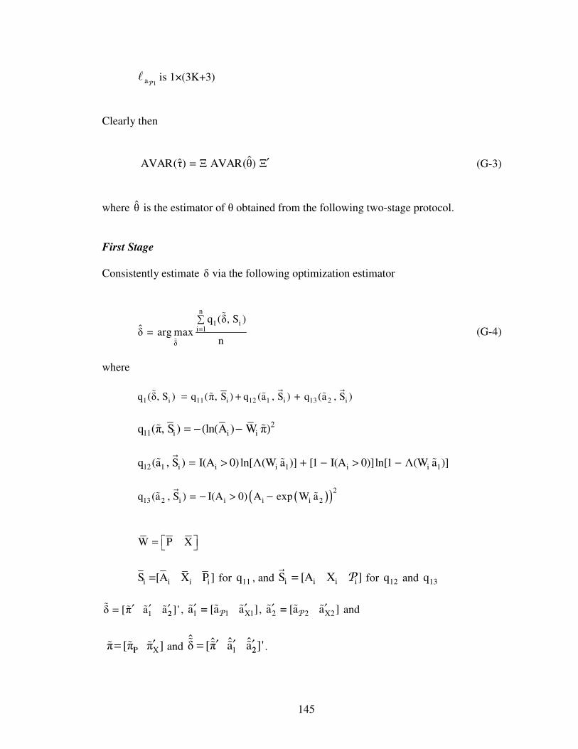
145

1a P

is 1×(3K+3)

Clearly then

ˆˆAVAR(τ) Ξ AVAR(θ) Ξ′= (G-3)

where θ is the estimator of θ obtained from the following two-stage protocol.

First Stage

Consistently estimate δ via the following optimization estimator

n

1 ii 1

δ

q (δ, S )δ = arg max

n=

∑

(G-4)

where

1 i 11 i 12 1 i 13 2 iq (δ, S ) q (π, S ) q (a , S ) q (a , S )= + +

2

11 i i iq (π, S ) (ln(A ) W π)= − −

12 1 i i i 1 i i 1q (a , S ) I(A 0) ln[Λ(W a )] [1 I(A 0)]ln[1 Λ(W a )]= > + − > −

( )( )2

13 2 i i i i 2q (a , S ) I(A 0) A exp W a= − > −

W P X =

i i i iS [A X P ]= for 11q , and i i i iS [A X ]=

P for 12q and 13q

1 22δ [π a a ] '′ ′ ′= , 1 1 X1a = [a a ]′ ′ P , 2 2 X2a = [a a ]′ ′

P and

1P Xπ [π π ]′= and 1 22

ˆ ˆ ˆˆδ [π a a ]'′ ′ ′= .

146

Second Stage

Consistently estimate γ via the following optimization estimator

n

ii 1

γ

ˆq(δ, γ, S )γ = arg max

n=

∑

(G-5)

where

i a i b i c iˆ ˆ ˆ ˆq(δ, γ, S ) q (δ, u, S ) q (δ, v, S ) q (δ, m , S )= + +

P

2a i i

ˆ ˆq (δ, u, S ) (U(δ, W ) u)= − −

2b i i

ˆ ˆq (δ, v, S ) (V(δ, W ) v)= − −

2c i i

ˆq (δ, m , S ) ( m )= − − P PP

1 2ˆ ˆ ˆˆδ [π a a ]'′ ′ ′= is the first stage estimator of δ , 1 1 X1ˆ ˆ ˆa = [a a ]′ ′

P and

2 2 X2ˆ ˆ ˆa = [a a ]′ ′P . Use 1q as shorthand notation for

1 11 12 1 13 2q (δ, S) q (π, S) q (a , S) q (a , S) = + +

where

2

11q (π, S) (ln(A) Wπ)= − −

12 1 1 1q (a , S) I(A 0)ln[Λ(Wa )] [1 I(A 0)]ln[1 Λ(Wa )]= > + − > −

( )( )2

13 2 2q (a , S) I(A 0) A exp Wa= − > −

S [A X P]= for 11q , and S [A X ]=

P for 12q and 13q ,

and use q as shorthand notation for

a b cq(δ,γ, S) q (δ, u, S) q (δ, v, S) q (δ,m , S)= + +P

147

where

2aq (δ, u, S) (U(a , W) u)= − −

2bq (δ, v, S) (V(a , W) v)= − −

2cq (δ, m , S) ( m )= − −P PP

with ˆAVAR(δ) being the asymptotic covariance matrix of the first stage estimator.45

Using well known results from asymptotic theory for two-stage estimators, we can show

that46

1 d2ˆ ˆAVAR(θ) n (θ θ) N(0, I)

−

− → (G-6)

where ˆˆ ˆθ = [δ γ ]′ ′ ′ , ˆplim(θ) = θ

11 12

12 22

D D

D DˆAVAR(θ)

= ′

(G-7)

11ˆAVAD R(δ)= (G-8)

3K×3K

[ ]12 δδ 1 δ 1 γ γγ

11E ED q q ' q E q

−−= ∇ ∇ ∇ ∇

[ ] [ ] [ ]δδ 1 δ 1 δ 1 δδ 1 γ

1

γ

1

δ

1

γE q q ' q q q qE E E E−− −

∇ ∇′ − ∇ ∇ ∇ ∇ (G-9)

45 Note that a consistent estimate ˆAVAR(δ) can be obtained from the packaged output

for the first stage estimator because the first stage estimator is unaffected by the fact that it is a component of a two-stage estimator. 46Discussions of asymptotic theory for two-stage optimization estimators can be found in Newey & McFadden (1994), White (1994, Chapter 6), and Wooldridge (2010, Chapter 12).

148

22 γγ γδ γ

1

δˆAVAR(γ) E E AVAR( )E 'ˆD q q δ q

− = = ∇ ∇ ∇

[ ]γ δ 1 δδ 1 γδ

1q ' q qE E E q

−∇ ∇

′ − ∇ ∇

[ ]γδ δδ 1 γ δ 1 γ

1

γ

1q q q ' q qE E E ' E

−− − ∇ ∇∇ ∇ ∇

1 1

γγ γ γ γγq q ' q qE E E− −

∇ ∇ ∇ + ∇ . (G-10)

Fortunately, (G-9) and (G-10) can be simplified in a number of ways. First note that we

can write

γ δ 1 γ δ 1q ' q q 'E E[ q | W]E∇ ∇ ∇ ∇ =

but

δ 1 δ 11 δ 12 δ 13q = q q q∇ ∇ + ∇ + ∇

with

δ 11 ( W π)Wq 2 ln(A ) 0 0 ∇ = −

1δ 12 aq [0 ln f (I(A 0) | W) 0]∇ = ∇ >

( )( ) ( )2δ 213 0 I(A 0) A exp Wa exp Waq W0 2 ∇ = > −

where

I(A 0) [1 I(A 0)]1 1Λ(W a ) [1 Λ(Wa )f (I( | W ]A 0) ) > − >= −> .

Therefore

149

( )( ) ( )

1a

2

δ

2

1

2E ln(A )

E[ q | W,W] E[ ln f (I(A 0) |

( W π) | W W

I(A 0) A exp Wa exp Wa

W)]

E | W W2

′ − ∇ = ∇ > > −

= [ 0 0 0]

because 1aE[ ln f (I(A 0) | W)] 0∇ > = [see (13.20) on p. 477 of Wooldridge (2010)],

( )( ) ( )2 2I(A 0) A exp Wa exp Wa | WE 0 = > − , and ( W π) | WE ln(A ) 0 − = by

design.47 Finally, then we get

γ δ 1q ' qE 0 = ∇ ∇

so

[ ] [ ] [ ]12 δδ 1 δ 1 δ 1 δδ 1 γδ γγ

11 1E E E ED q q ' q q q qE

−− − ′ − = ∇ ∇ ∇ ∇ ∇ ∇ (G-11)

3K×3K 3K×3K 3K×3K 3K×3 3×3 3K×3 and

22 γγ γδ γδ γγ

1 1ˆˆAVAR(γ) E E AVAR(δ) E 'ED q q q q− −

= ∇ ∇ ∇ = ∇

3×3 3×3K 3K×3K 3K×3 3×3

1 1

γγ γ γ γγq q ' q qE E E− −

∇ ∇ ∇ + ∇ . (G-12)

3×3 3×3 3×3 3×3 so

47 The last result warrants some discussion. We are assuming here that the correct model specification is the unrestricted two-part model detailed in (3-5) through (3-7). We also assume that, although (3-4) is not correctly specified in a causal sense, it can, nonetheless be viewed as a “best predictor” model in which the best predictor (the conditional mean

of (ln(A) | P, X) is assumed to be equal to p XW π Pπ Xπ= + . This implies that

( W π) | WE ln(A ) 0 − = .

150

11 1

(3K 3) (3K

2

12 23) 2

D D

3K 3K 3K 3

D D

3 3K

ˆAVAR(

3 3

θ)+ × +

× × = ′

× ×

.

Let’s consider each of the individual components of (G-9) and (G-10) in turn.

1δ 1δ qE[ ]−−−−∇∇∇∇

3K×3K

Written out explicitly we have

1 1

2 2

1ππ 11

δδ 1 a 11 1

a 2

1a a 13

E[ q ] 0 0

q ] 0 E[ q ] 0

0 0

[

E[ q ]

E

−

−

− −

∇ ∇ = ∇ ∇

. (G-13)

Now

π 11q 2 ln(A)( Wπ)W∇ = −

and

ππ 11q W2 W∇ = ′− .

Therefore

ππ 11E[ q ] E W W2 ∇ = − ′ . (G-14)

A consistent estimator of 1ππ 11E[ q ]−∇ is

1

n1

ππ 11i 12

i i

1E[ ] 2

nWq W

−

−

=

∑ ′

∇ = −

151

i

1n

2i

i1

W Wn 2−

=

∑

= ′− . (G-15)

where π is the OLS estimator of π in the AGG-LOG model and 2n is the size of the

aggregated sample. Similarly,

1 1

11 1aa 2E ˆAV[ ] )q AR(a− = −∇ (G-16)

= the negative of the asymptotic covariance matrix for first stage, first

part, logit estimation of 1α in the unrestricted two-part estimation

protocol culminating in (14). We get an estimate of this directly

from the Stata output.

A consistent estimator of 1 1 2a a 1

1E[ q ]−∇ is

1 1

11a 1a 2

ˆ ˆnAVAR *(aE q ] )[ − = −∇ (G-17)

where 1ˆAVAR *(a ) is the estimated variance-covariance matrix output by the Stata logit

procedure. Also

( )( ) ( )2 13a 2 2I(A 0) A exp Wa expq 2 Wa W∇ > −=

and

( )( ) ( ) ( )2 2a 2a 213 2I(A 0) A exp Wa exp Wa exp Wa W Wq 2 ′> − − ∇ = − .

Therefore

152

( )( ) ( ) ( )2 2a 13a 2 2 2I(A 0) A exp Wa exp Wa exp Wa W[ 2E WE q ] ′> − −

∇ = .

(G-18)

A consistent estimator of 2 2 3a

1a 1E[ q ]−∇ is

( )( ) ( )

( )2 2

1

n1

a 13i 11

i i i 2 i 2

a

i 2 i i

I(A 0) A exp W a exp W a1E[ q ] 2

exp W a W Wn

−

−

=∑

∇ =

> − −

′

( )( ) ( )

( )

i i i 2 i 2

i 2 i

1

n

1i 1

i

I(A 0) A exp W a exp W a

exp W a Wn 2

W

−

=∑

> − −

′ =

.

(G-19)

where 2a is the first stage, second part, estimator of 2a , and 1n is the size of the

subsample for whom I(A 0) 1> =

so

1 1

2 2

1ππ 11

δδ 1 a a 12

1a 1

1

3

1

a

[ q ] 0 0

q ] 0 [ q ] 0

0

E

ˆ ˆE[ E

ˆ ]E0 [ q

−

−

−

− ∇ ∇ = ∇ ∇

. (G-20)

δ 1 δ 1q ' qE ∇ ∇∇ ∇∇ ∇∇ ∇

3K×3K Written out explicitly we have

[ ]1 2

1 1 1 1 2

2 2 1 2 2

π 11 π 11 π 11 a 12 π 11 a 13

δ 1 δ 1 a 12 π 11 a 12 a 12 12 13

a 13 π 11 a 1

a a

a3 a 12 a 13 13

E[ q ' q ] E[ q ' q ] E[ q ' q ]

q ' q E[ q ' q ] E[ q ' q ] E[ q ' q ]

E[ q ' q ] E[ q ' q ] E[ q ' q ]

E

∇ ∇ ∇ ∇ ∇ ∇

∇ ∇ ∇ ∇ ∇ ∇ ∇ ∇

∇ ∇ ∇ ∇ ∇ ∇

=

.

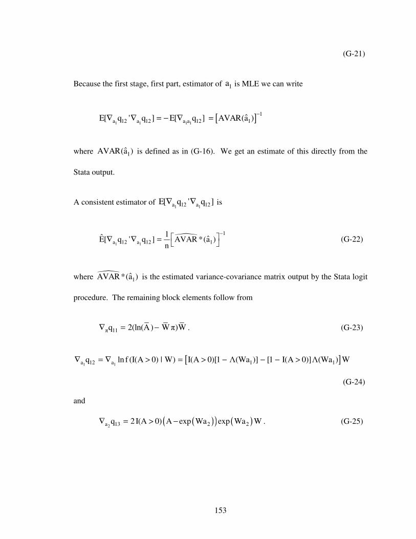
153

(G-21)

Because the first stage, first part, estimator of 1a is MLE we can write

[ ]1 1 1 1a 12 12 a

1

a 112aE[ q ' q ] E[ ˆAVARq ] (a )−

∇ ∇ − ∇ ==

where 1ˆAVAR(a ) is defined as in (G-16). We get an estimate of this directly from the

Stata output.

A consistent estimator of 1 1a 12a12E[ q ' q ]∇ ∇ is

1 1

1

aa 12 12 1

1ˆAVARE[ q ' *(a )

nq ]

− =

∇ ∇ (G-22)

where 1ˆAVAR *(a ) is the estimated variance-covariance matrix output by the Stata logit

procedure. The remaining block elements follow from

π 11q 2 ln(A)( Wπ)W∇ = − . (G-23)

[ ]1 112a a 1 1q ln f (I(A 0) | W) I(A 0) Wa )] [1[1 Λ( I(A 0)] Wa ) WΛ(−∇ = ∇ > = > − − >

(G-24) and

( )( ) ( )2 13a 2 2I(A 0) A exp Wa expq 2 Wa W∇ > −= . (G-25)

154

where the formulation of 1 2a 1q∇ comes from equation (16.4.8) on p. 350 of Fomby et al.

(1984) and Λ( ) denotes the logistic cdf. The remaining required consistent matrix

estimators are

2n

π 11 π 11 π 11j π 11jj 12

1ˆ ˆ ˆE[ q ' q ] q ' qn =

∑∇ ∇ = ∇ ∇ (G-26)

1 1

n* *

π 11 12 π 11i1

a ii

a 12

1ˆ ˆ ˆE[ q ' q ] q ' qn =∑∇ ∇ = ∇ ∇ (G-27)

2 2

n* *

π 11 13 π 11i 13ii 11

a a

1ˆ ˆ ˆE[ q ' q ] q ' qn =

∑∇ ∇ = ∇ ∇ (G-28)

1 2 1 2

n

a 12 a 13 12i 13ii 11

a a

1ˆ ˆ ˆE[ q ' q ] q ' qn =

∑∇ ∇ = ∇ ∇ (G-29)

2 2 2 2

n

a 13 a 13 a 13i a 13ii 11

1ˆ ˆ ˆE[ q ' q ] q ' qn =

∑∇ ∇ = ∇ ∇ (G-30)

where

π 11i i i iq 2 ln( ˆ( W ) WA ) π∇ = − (G-31)

[ ]1 1a 12i i i i i 1 i

ˆ ˆW a )q I(A 0)[1 Λ( I(A 0)]Λ] [1 W a W( )∇ = −> >−− (G-32)

and

( )( ) ( )2 i i 2a 13i i ii 2

ˆ ˆI( 0) Aq 2 exp W a exp W WA a> −∇ = (G-33)

The components of equations (G-27) and (G-28) are obtained using

* *i i

*π 11i iq 2 ln(( W πA W) )∇ = − .

where

*i i iW [P X ]= denotes the observation on W [P X]= that pertains to the ith

individual in the sample (i = 1, ..., n) for the relevant aggregation unit

(j = 1, ..., 2n )

155

so

[ ]

1 2

1 1 1 1 2

2 2 1 2 2

π 11 π 11 π 11 a 12 π 11 a 13

δ 1 δ 1 a 12 π 11 a 12 a 12 a 12 a 13

a 13 π 11 a 13 a 12 a 13 a 13

[ q ' q ] [ q ' q ] [ q ' q ]

q ' q [ q ' q ] [ q ' q ] [ q ' q ]

[ q ' q ] [ q

ˆ ˆ ˆE E E

' q ] [ q ' q ]

ˆ ˆ ˆ ˆE E E E

ˆ ˆ ˆE E E

∇ ∇ ∇ ∇ ∇ ∇ ∇ ∇ ∇ ∇ ∇ ∇ ∇ ∇ ∇ ∇ ∇ ∇ ∇

=

∇

.

(G-34)

γδqE ∇∇∇∇

3×3K Written out explicitly we have

γ u a v b m cq = [( q 0 0) (0 q +0) (0 0 q )]∇ ∇ + + +∇ + +∇P

v mu a b c[ q q q ] ∇ ∇ ∇=P

( ) ( ) i2 U(a, W) u V(a, W) v ( m )= − − − PP (G-35)

and

1 2

1 2

1 2

uα αuπ a a u a

γδ vπ b v b vα α

m

b

π c cm cα m α

E[ q ] E[ q ] E[ q ]

E[ q] = E[ q ] E[ q ] E[ q ]

E[ q ] E[ q ] E[ q ]

∇ ∇ ∇

∇ ∇ ∇ ∇

∇ ∇ ∇ P P P

1 2

1 2

π a a

π a a

E[ U] E[ U] E[ U]

= 2 E[ V] E[ V] E[ V]

0 0 0

∇ ∇ ∇

∇ ∇ ∇

(G-36)

where

π π 0U V∇ = ∇ = . (G-37)

1 1a 1 22Λ(Wa )λ(Wa )exp(Wa ) WU =∇ (G-38)

2

2a 1 2Λ(Wa ) exp(Wa )WU =∇ . (G-39)

156

1a 1 2λ(Wa ) exp(Wa ) WV∇ = (G-40)

and

2a 1 2Λ(Wa )exp(Wa ) WV∇ = . (G-41)

Note that

aΛ(a) λ(a) Λ(a)[1 Λ(a)]∇ = = −

aλ(a) λ(a)[1 2Λ(a)]∇ = − .

The requisite consistent matrix estimators are

π πˆ ˆE[ U] E[ V] = 0∇ = ∇ (G-42)

1 1

n

ai 1

a iE[ U] = U

=∑∇ ∇ (G-43)

2 2a

n

i 1a i

E[ U] = U=∑∇ ∇ (G-44)

1 1a

n

i 1a i

E[ V] = V=∑∇ ∇ (G-45)

and

2 2

n

ai 1

a iE[ V] = V

=∑∇ ∇ (G-46)

where

π πi iU V = 0∇ = ∇ (G-47)

1a 1 1 2i i i ii

2Λ(W )λ(W ) exp(ˆ ˆ ˆU a a aW ) W∇ = (G-48)

2a i ii

21 2Λ(W ) exp(Wˆ ˆa ) WU a=∇ (G-49)

1a 1 2i i ii

λ(W )ˆ ˆV = a aexp(W ) W∇ (G-50)

157

and

2a 1 2i i ii

Λ (W )ˆ ˆV = a aexp(W ) W∇ (G-51)

so

1 2

1 2

a a

γδ a a

ˆ ˆ0 E[ U] E[ U]

ˆ ˆ ˆE[ q] = 2 0 E[ V] E[ V]

0 0 0

∇ ∇ ∇ ∇ ∇

. (G-52)

γγ1E[ q]−−−−∇∇∇∇

3×3

[ ]

[ ]

1

1 1

uu a

γ

m

γ

cm

vv b

1

E 0 0

E 0 E 0

q0

q

q

E

q

0

−

− −

−

∇

∇ ∇

∇

=

P P

(G-53)

because uv a vu b um a vm m u mb c cvq q q q q q 0∇ = ∇ =∇ =∇ =∇ =∇ =P P P P

. Now

uu a vv b m m cq q q 2∇ = ∇ = ∇ = −P P

therefore

1

γγ

10 0

2

1E 0 0

2

10

q

02

−

− = −

∇

−

. (G-54)

γ γq' qE ∇ ∇∇ ∇∇ ∇∇ ∇

3×3

Given that

158

( ) ( ) iγ 2 U(a, W) u V(a,q W) v ( m )= −∇ − − PP . (G-55)

we have

γ γq ' qE ∇ ∇ =

2

2

2

E[(U(a, W) u)E[(U(a, W) u)E[(U(a, W) u) ]

( m )](V(a, S) v)]

E[(V(a, S) v)E[(U(a, W) u)4 E[(V(a, S) v) ] .

( m )](V(a, S) v)]

E[(U(a, W) u) E[(V(a, S) v)E[( m ) ]

( m )] ( m )]

−− −

−− −−

− −−

− − −

− −

P

P

P

P P

P

P

PP P

(G-56)

The corresponding consistent estimator is

n n ni2 ii

i 1 i 1 i 1ii

n n ni 2 ii

i 1 i 1 i 1ii

γ

i

γ

n

i 1i

ˆ ˆˆ(U u) ˆ(U u)1 1 1ˆ ˆ(U u)ˆn n n ˆ( m )ˆ(V v)

ˆ ˆˆ(U u) ˆ(V v)1 1 1ˆ ˆ ˆE 4 (V v)ˆn n n ˆ( m )ˆ(V v)

ˆ ˆ(U u)1

n ˆ( m )

q ' q

= = =

= = =

=

∑ ∑ ∑

∑ ∑ ∑

∑

− −− −−

− − = − −−

− −

∇ ∇

P

P

P

P

P

P

n n2i

ii 1 i 1

i

.

ˆ ˆ(V v)1 1ˆ( m )

n nˆ( m )= =∑ ∑

− − − P

P

PP

(G-57)

Based on (G-8), (G-11) and (G-12) and using the two-stage estimator θ we can

consistently estimate (G-7) as

11 12

12 22

ˆ ˆD D

ˆ ˆD D

ˆAVAR(θ)

= ′

where

2

111

1 2

ˆn AVAR *(π)

ˆ ˆAVAR(δ) nAVAR *(a )

ˆn AVAR *(a )

0 0

D 0 0

0 0

=

=

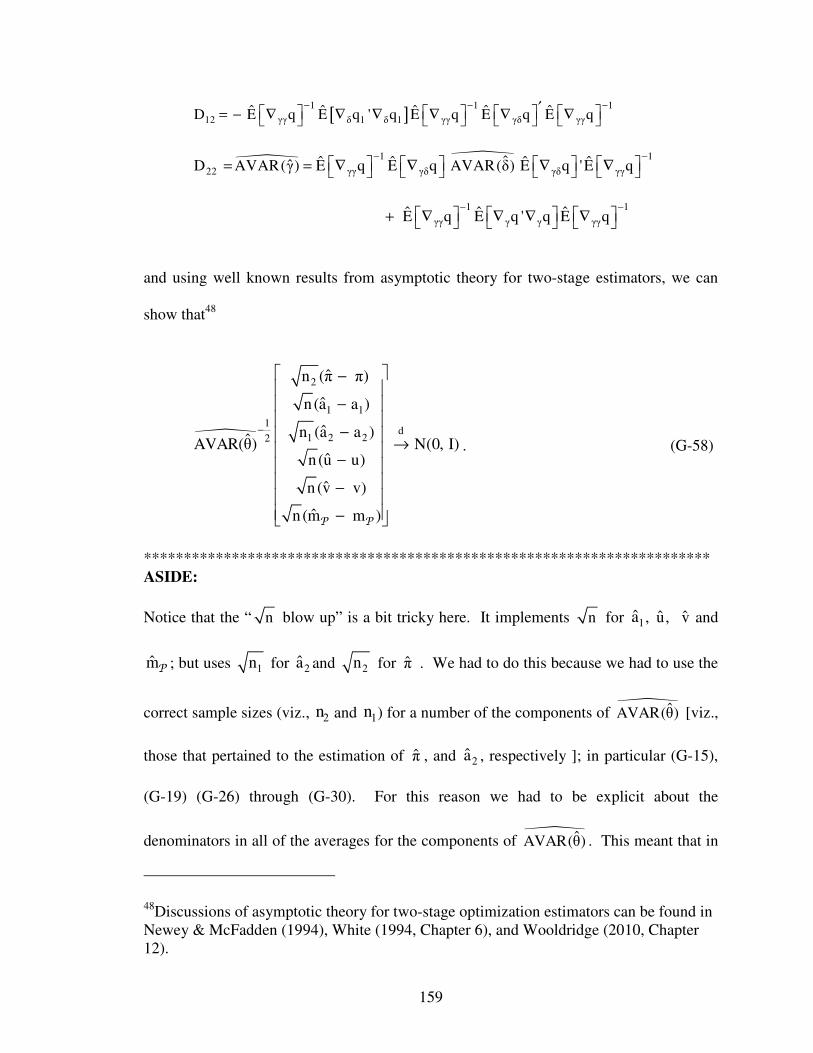
159

[ ]12 γγ δ 1 δ 1 γγ γδ γ

1 1

γ

1ˆ ˆ ˆ ˆ ˆE E E E ED q q ' q q q q− − −′ = ∇ ∇ ∇ ∇ ∇ ∇ −

22 γγ γδ γδ γ

1

γ

1ˆ ˆ ˆ ˆˆAVAR(γ) E E AVAR( ) EˆD q q δ q q'E− −

= ∇ ∇ ∇ = ∇

γγ γ γ γγ

1 1q q ' q qˆ ˆ ˆE E E

− −∇ ∇ ∇ + ∇

and using well known results from asymptotic theory for two-stage estimators, we can

show that48

2

1 1

1d

1 2 22

ˆn (π π)

ˆn (a a )

ˆn (a a )ˆAVAR(θ) N(0, I)ˆn (u u)

ˆn (v v)

ˆn (m m )

−

−

−

− →

− − − P P

. (G-58)

*********************************************************************** ASIDE:

Notice that the “ n blow up” is a bit tricky here. It implements n for 1a , u, v and

mP ; but uses 1n for 2a and 2n for π . We had to do this because we had to use the

correct sample sizes (viz., 2n and 1n ) for a number of the components of AVAR(θ) [viz.,

those that pertained to the estimation of π , and 2a , respectively ]; in particular (G-15),

(G-19) (G-26) through (G-30). For this reason we had to be explicit about the

denominators in all of the averages for the components of AVAR(θ) . This meant that in

48Discussions of asymptotic theory for two-stage optimization estimators can be found in Newey & McFadden (1994), White (1994, Chapter 6), and Wooldridge (2010, Chapter 12).

160

the construction of the requisite asymptotic t-stats we had to explicitly include the “blow-

up” in the numerator (i.e., we had to multiply by the square-root of the appropriate

sample size). I refer to this as “tricky” because one typically does not have to do this. In

the usual asymptotic t-stat construction the denominators of the averages (“n”) need not

be included in the construction of the asymptotic covariance matrix because it typically

manifests as a multiplicative factor and, after pulling the diagonal and taking the square

root to get the standard errors, this multiplicative n cancels with the “blow-up” factor in

the numerator. For example, the asymptotic t-stat of the OLS estimator is

( ) ( )

k k k k k k k k

1 1 12 22 kk kk

kk

ˆ ˆ ˆ ˆn (ρ ρ ) n (ρ ρ ) n (ρ ρ ) (ρ ρ )

ˆAVAR(ρ) ˆ ˆn σ σ1σ

n

− − −

− − − −= = =

′ ′ ′

XX XXXX

where

n is the sample size

kρ is the coefficient of the kth regressor in the linear regression

kρ is its OLS estimator

2σ is the regression error variance estimator

X is the matrix of regressors

and kk′XX is the kth diagonal element of ′XX . Note how the “ n s” simply cancel.

Note also that what we typically refer to as the “asymptotic standard error” can actually

be written as the square root of the diagonal element of the consistent estimator of the

asymptotic covariance matrix divided by n; in other words

161

asy std err = AVAR(ρ)

n.

************************************************************************

Now back to the issue at hand. Moreover

2 P P

1 1

1 d1 2 22

ˆn (π π )

ˆn(a a )

ˆn (a a )ˆAVAR(τ) N(0, I)

ˆn(u u)

ˆn(v v)

ˆn (m m )

−

−

−

− →

− − −

P P

P P

P P

. (G-59)

where

ˆAVAR(τ) ΞAVAR(θ) Ξ '= (G-60)

and τ and Ξ are defined as in (G-2). Now combining (G-1) with (G-59) and (G-60) we

get

( ) ( )

1d

AL UPO AL UPO AL UPO2ˆ ˆ ˆ ˆavar(η η ) n η η η η N(0, I)−

− − − − → (G-61)

where

AL UPOˆ ˆ ˆ ˆ ˆavar(η η ) c(τ) AVAR(τ) c(τ) '− =

and

21 1 1 2

ˆ ˆu uˆ ˆ ˆ ˆ ˆ ˆ ˆ ˆˆ ˆ ˆ ˆc(τ) 1 m 1 m m a / v m a u/ v 1 a a

ˆ ˆv v

= − − − − − − +

P P P P P P P P .

162

Appendix H.

Asymptotic Distribution (and Standard Error) of UPOLη in Eqn (4-6)

We may write UPOLη as

UPOL κη

ν=

where

n

ii 1

1ˆ ˆκ (α, W )

n=∑=

K

n

ii 1

1ˆ ˆν = (α, W )

n=∑

V

Using the corresponding consistent estimators for k , and v say

1 2 P1 1 2 P2(α, W) λ(Wα ) exp(Wα )α Λ(Wα ) exp(Wα )α+=

K

1 2(α, W) Λ(Wα ) exp(Wα )=

V

P is the logged prices of alcohol

1 2ˆ ˆ ˆα [α α ]'′ ′= (with 1 P1 X1

ˆ ˆ ˆα = [α α ]′ ′ and 2 P2 X 2ˆ ˆ ˆα = [α α ]′ ′ ) is the consistent

estimate of the parameter vector 1 2α [α α ]'′ ′= (with 1 P1 X1α = [α α ]′ ′ and

2 P2 X2α = [α α ])′ ′ ) [the parameters of equation (4-6)] obtained via the

two-part protocol culminating in (4-4) using logged prices of alcohol

and i i iW [P X ]=

denotes the observation on W [P X]=

for the ith individual in the

sample

163

(i = 1, ..., n). Let ˆ ˆγ = [κ ν ]′ and γ = [κ ν ]′ , where ˆplim[γ] = γ . If we could show

that

1 d2ˆ ˆAVAR(γ) n (γ γ) N(0, I)

−

− →

where the formulation of ˆAVAR(γ) is known, then we could apply the δ-method to

obtain the asymptotic variance of UPOLη as

UPOLˆ ˆavar(η ) c(γ) AVAR(γ) c(γ) '=

where 2c(γ) [1/ ν κ / ν ]= − . Moreover, if we have a consistent estimator for

ˆAVAR(γ) , say AVAR(γ) [i.e. ˆp lim AVAR(γ) AVAR(γ) =

], then we could

consistently estimate UPOLˆavar(η ) as

UPOLˆ ˆ ˆ ˆavar(η ) c(γ) AVAR(γ) c(γ) '= . (H-1)

We focus, therefore, on finding the asymptotic distribution of γ and, in particular, the

formulation of its asymptotic covariance matrix.

First, let θ = [δ γ ]′ ′ ′ where 1 2δ [α α ]'′ ′= , γ [κ ν ]′ = (recall, 1 P1 X1α = [α α ]′ ′

and 2 P2 X2α = [α α ]′ ′ ), and note that γ can be viewed as the second stage estimator in the

following two-stage protocol

First Stage

Consistently estimate δ via the following optimization estimator

164

n

1 ii 1

δ

q (δ, S )δ = arg max

n=∑

(H-2)

where

1 i 11 1 i 12 2 iq (δ, S ) q (α , S ) q (α , S )= +

11 1 i i i 1 i i 1q (α , S ) I(A 0) ln[Λ(W α )] [1 I(A 0)] ln[1 Λ(W α )]= > + − > −

( )( )2

12 2 i i i i 2q (α , S ) I(A 0) A exp W α= − > −

i i iS [A X ]=

1 22δ [α α ]'′ ′= , 1 P1 X1ρ = [ρ ρ ]′ ′ and 2 P2 X2ρ = [ρ ρ ]′ ′ and 1 22

ˆ ˆ ˆδ [ρ ρ ]'′ ′=

Second Stage

Consistently estimate γ via the following optimization estimator

n

ii 1

γ

ˆq(δ, γ, S )γ = arg max

n=

∑

(H-3)

where

i a i b iˆ ˆ ˆq(δ, γ, S ) q (δ, κ, S ) q (δ, ν, S )= +

2a i i

ˆ ˆq (δ, κ, S ) ( (α, W ) κ)= − −

K

2b i i

ˆ ˆq (δ, ν, S ) ( (α, W ) ν)= − −

V

δ is the first stage estimator of δ . Use 1q as shorthand notation for

1 11 1 12 2q (δ, S) q (α , S) q (α , S)= +

165

with

11 1 1 1q (α , S) I(A 0) ln[Λ(W α )] [1 I(A 0)]ln[1 Λ(W α )]= > + − > −

( )( )2

12 2 2q (α , S) I(A 0) A exp W α= − > −

S [A X ]=

and use q as shorthand notation for

a bq(δ,γ, S) q (δ, κ, S) q (δ, ν, S)= +

with

2aq (δ, κ, S) ( (α, W) κ)= − −

K

2bq (δ, ν, S) ( (α, W) ν)= − −

V

and let ˆAVAR(δ) denote the asymptotic covariance matrix of the first stage estimator.49

Using well known results from asymptotic theory for two-stage estimators, we can show

that50

1 d2ˆ ˆAVAR(γ) n (γ γ) N(0, I)

−

− → (H-4)

where, ˆplim(γ) = γ

49 Note that a consistent estimate ˆAVAR(ρ) can be obtained from the packaged output

for the first stage estimator because the first stage estimator is unaffected by the fact that it is a component of a two-stage estimator. 50Discussions of asymptotic theory for two-stage optimization estimators can be found in Newey & McFadden (1994), White (1994, Chapter 6), and Wooldridge (2010, Chapter 12).

166

δ δ

1

γγ γ γq q qˆˆAVAR(γ) E E AVAR(α)E− ′ = ∇ ∇ ∇

[ ]δ 1 δδγ 1 δ

1

γq ' q qE E E q−

∇ ∇′ − ∇ ∇

δ δ 1 δ 1

1 1

γ γ γ γγq q qE q qE'E E− −′ − ∇

∇ ∇ ∇ ∇

1 1

γγ γ γ γγq q ' q qE E E− −

∇ ∇ ∇ + ∇ (H-5)

Fortunately, (H-5) can be simplified in a number of ways. Note that we can write

γ γδ 1 δ 1q ' q qE 'E[ q | W]E∇ ∇ ∇ ∇ =

but

1 11 12δ δ δq = q q∇ ∇ +∇

with

1δ 11 αq [ ln f (I(A 0) | W) 0 ]∇ = ∇ >

( )( ) ( )2δ 212 I(A 0) A exp W α expq 0 W α2 W ∇ = >

−

where

I(A 0) [1 I(A 0)]1 1Λ(W α ) [1 Λ(f (I( W αA ) | W) )]0 > − >> = −

.

Therefore

( )( ) ( )

1α

2

δ

2

1

E[ ln f (I(A 0) | W)]

WI(A 0) A exp Wα ex

E[p Wα | W

q | ]2 WE

′ ∇ > ∇ =

> −

= [ 0 0]

167

because 1α

E[ ln f (I(A 0) | )] 0W∇ > =

[see (13.20) on p. 477 of Wooldridge (2010)] and,

( )( ) ( )2 2I(A 0) A exp W α exp W α | WE 0 =>−

by design. Finally, then we get

γ δ 1q ' qE 0 = ∇ ∇

so

γγ γδ γδ γ

1

γ

1ˆAVAR( ) E E Aγ q VAR(α) Eq q 'E q

− −∇ ∇ ∇ ∇ =

3×3 3×2K 2K×2K 2K×3 3×3

1 1

γγ γ γ γγq q ' q qE E E− −

∇ ∇ ∇ + ∇ . (H-6)

3×3 3×3 3×3 Let’s consider each of the individual components of (H-6) in turn.

δ1

δ 1qE[ ]−−−−∇∇∇∇

2K×2K

Written out explicitly we have

1 1

2 2

1

1αα

α α 11

1 1α 12α

E[ q ] 0q ]

0 E[

[E

q ]−

−

− ∇ ∇ = ∇

. (H-7)

Now

1 1

11 1αα 1E ˆAV[ ] )q AR(α− = −∇ (H-8)

= the negative of the asymptotic covariance matrix for first

stage, first part, logit estimation in the two-stage estimation

protocol for θ. We get an estimate of this directly from the Stata

output.

168

A consistent estimator of 1 1 1α α 1

1E[ q ]−∇ is

1 1

11α 1α 1

ˆ ˆnAVAR *(αE q ] )[ − = −∇ (H-9)

where 1ˆAVAR * (α ) is the estimated variance-covariance matrix output by the Stata logit

procedure. Also

( )( ) ( )2 2α 212 I(A 0) A eq xp Wα W W2 exp α∇ = > −

and

( )( ) ( ) ( )2 2α 2 2 2α 12 I(A 0) A exp Wα exp Wαq exp Wα W W2 ′> − −∇

=

.

Therefore

( )( ) ( ) ( )2 2α 12α 2 2 2I(A 0) A exp Wα exp WαE[ exp WE αq W2 W] ′> − −

∇ =

.

(H-10)

A consistent estimator of 2 2 2α

1α 1E[ q ]−∇ is

( )( ) ( ) ( ) 2 2 i i i 2 i 2

1n

1α α 12 1

i 1i 2 i iI(A 0) A exp W α exp W α exp W α WE[ q ] n 2 W

−−

=

∑ ′> − −

∇ =

(H-11)

where 1n is the size of the subsample for whom I(A 0) 1> = , so

169

1 1

2 2

1α1 1

αα

α

α 11

δδ 1 1 1α 12

[ qEˆ ˆE[ E[

E

] 0q ] q ]

0 [ q ]−

−

− − ∇ ∇ = ∇ = ∇

. (H-12)

δ 1 δ 1q ' qE ∇ ∇∇ ∇∇ ∇∇ ∇

2K×2K Written out explicitly we have

[ ] 1 1 1 2

2 1 2 2

α 11 α 11 α 11 α 12

α 1 α 1α 12 α 11 α 12 α 12

E[ q ' q ] E[ q ' q ]q ' q

E[ q ' q ] E[ q ' q ]E =

∇ ∇ ∇ ∇ ∇ ∇

∇ ∇ ∇ ∇ . (H-13)

Because the first stage, first part, estimator of 1ρ is MLE we can write

[ ]1 1 1 1α 11 α 11 α α

1

111E[ q ' q ] E[ ˆAVARq ] (α )−

∇ ∇ − ∇ ==

= the inverse of the asymptotic covariance matrix for first stage,

first part, logit estimation in the two-stage estimation

protocol for θ. We get an estimate of this directly from the Stata

output.

A consistent estimator of 1 1α 11 α 11E[ q ' q ]∇ ∇ is

1 1

1

α α11 11 1

1ˆAVARE[ q ' *(α )

nq ]

− =

∇ ∇ (H-14)

where 1ˆAVAR * (α ) is the estimated variance-covariance matrix output by the Stata logit

procedure. The remainder of the block elements follow from

170

1 111α α 1 1q ln f (I(A 0) | W) I(A W0)[1 Λ( I(A 0α )] [1 Wα ) W)]Λ(∇ = ∇ > = > − − − >

(H-15)

( )( ) ( )2α 2 212 I(A 0) A eq xp Wα W W2 exp α∇ = > −

. (H-16)

where the formulation of 1 1α 1q∇ comes from equation (16.4.8) on p. 350 of Fomby et al.

(1984) and Λ( ) denotes the logistic cdf. The remaining required consistent matrix

estimators are:

1 2 1 2

n

α 11 α 12 α 11i α 12ii 11

1ˆ ˆ ˆE[ q ' q ] q ' qn =

∑∇ ∇ = ∇ ∇ (H-17)

2 2 2 2

n

α 12 α 12 α 12i α 12ii 11

1ˆ ˆ ˆE[ q ' q ] q ' qn =

∑∇ ∇ = ∇ ∇ (H-18)

where

1α 11i i i i i 1 i1W )]ˆ ˆ ˆq I(A 0)[1 Λ( α I(A 0[1 W ) W)]Λ( α∇ = − − > − >

(H-19)

and

( )( ) ( )2 i i 2 iα 12i i i2

ˆ ˆI( 0) A exp W α exp Wq 2 α WA > −∇ =

(H-20)

so

1 1 1 2

2 1 2 2

11 11 11 12

1 1 1 1δ δ

12 11

ρ ρ ρ ρ

ρ ρ

ρ 12 1ρ ρ 2ρ

[ q ' q ] [ q ' q ]q ' q q ' q

[ q ' q ] [ q

ˆ ˆE Eˆ ˆ

'E E

ˆ ˆE E q ]

∇ ∇ ∇ ∇ ∇ ∇ ∇ ∇ ∇ ∇ ∇ ∇

= =

.

(H-21)

γδqE ∇∇∇∇

2×2K Written out explicitly we have

171

γ κ a ν bq = [( q 0) (0 q ) ]∇ ∇ + +∇

κ a ν b[ q q ] ∇ ∇=

( ) ( )2 (α, W) κ (α, W) ν = − −

K V (H-22)

and

1 2

1 2

κα a κα a

γδ

να b να b

E[ q ] E[ q ]E[ q] =

E[ q ] E[ q ]

∇ ∇ ∇

∇ ∇

1 2

1 2

α α

α α

E[ ] E[ ]= 2

E[ ] E[ ]

∇ ∇

∇ ∇

K K

V V (H-23)

where

1α 1 1 P1 1 2λ(W α )[1 2Λ(W α )]α W λ(W α )[1 0 ... 0]exp(W α )∇ = − +

K

1 2 P2λ(W α ) exp(W α )α W+

1 2 1 P1 P2λ(Wα )exp(Wα ) [1 2Λ(Wα )]α + α W [1 0 ... 0] = − +

(H-24)

2α 1 2 P1 1 2 P2 2λ(W α ) exp(W α )α W + Λ(W α )exp(W α )α W exp(W α )[1 0 ... 0]=∇ +

K

2 1 P1 1 P2 1exp(Wα ) λ(Wα )α + Λ(Wα )α W Λ(Wα )[1 0 ... 0] = +

.

(H-25)

1α 1 2λ(Wα )exp(Wα ) W∇ =

V (H-26)

and

2 1α 2Λ(Wα )exp(Wα ) W∇ =

V . (H-27)

The following equalities were used in deriving the above results

172

aΛ(a) λ(a) Λ(a)[1 Λ(a)]∇ = = −

aλ(a) λ(a)[1 2Λ(a)]∇ = − .

The requisite consistent matrix estimators are

1 1

n

iαi

α1

E[ ] ==∑∇ ∇K K (H-28)

2 2

n

iαi

α1

E[ ] ==∑∇ ∇K K (H-29)

1 1

n

iαi

α1

E[ ] ==∑∇ ∇V V (H-30)

and

2 2

n

iαi

α1

E[ ] ==∑∇ ∇V V (H-31)

where

1 iα 1 2 1 P1 Pi i i2i

ˆ ˆλ(W )exp(W ) [1 2Λ(W )]α + α ˆ ˆ ˆα α W [1 0 ...α 0] = − + ∇

K

(H-32)

2 2 1 P1 1 Pα i 2i ii 1i i

ˆ ˆexp(W ) λ(W )α + Λ(W )α W Λ(W )[1 0 ..ˆ ˆ . 0ˆ ˆα ]α α α = ∇ +

K

(H-33)

1 1 2α i i ii

λ(W )exp(Wˆ ˆ= α α ) W∇

V (H-34)

and

1 1 2α i i ii

Λ(W )exp(Wˆ ˆ= α α ) W∇

V . (H-35)

so

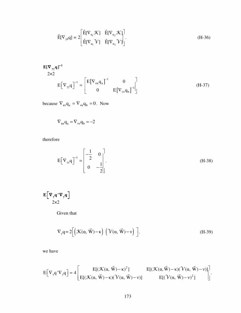
173

1 2

1 2

α α

γδ

α α

ˆ ˆE[ ] E[ ]E[ q] = 2

ˆ ˆE[ ] E[ ]

∇ ∇ ∇ ∇ ∇

K K

V V. (H-36)

γγ1E[ q]−−−−∇∇∇∇

2×2

[ ]

[ ]

1

κκ aγγ

νν

1

b

1 E 0E

qq

q0 E

−−

−

∇∇

∇ =

(H-37)

because κν a νκ bq q 0∇ = ∇ = . Now

κκ a νν bq q 2∇ = ∇ = −

therefore

1

γγ

10

2E

10

q

2

−

−

=

∇−

. (H-38)

γ γq' qE ∇ ∇∇ ∇∇ ∇∇ ∇

2×2

Given that

( ) ( )γ 2 (α, W) κ (α, Wq ) ν = − −

∇

K V . (H-39)

we have

γ 2γ

2E[( (α, W) κ) ] E[( (α, W) κ)( (α, W) ν)]E 4

E[( (α, W) κ)( (α, W) ν)] E[( (α, W) ν)q ' q

]

− − − =

− − −∇

∇

K K V

K V V.

174

(H-40) The corresponding consistent estimator is

n n2

i i ii 1 i 1

γ γn n

2i i i

i 1 i 1

1 1 ˆˆ ˆˆ ˆ ˆ( κ) ( κ)( ν)n n

E 41 1ˆ ˆˆ ˆ ˆ ˆ( κ)( ν

q ' q

) ( ν)n n

= =

= =

∑ ∑

∑ ∑

− − −

= − − −

∇ ∇

K K V

K V V

. (H-41)

Based on the above results, we can consistently estimate (H-5) as

1 1

γγ γ γ γδ δ γˆ ˆ ˆ ˆˆˆAVAR(γ) E E Aq q qVAR(α) qE E

− −′ ∇ = ∇ ∇ ∇

1 1

γγ γ γ γγq q ' q qˆ ˆ ˆE E E− −

∇ ∇ ∇ + ∇

and using well known results from asymptotic theory for two-stage estimators, we can

show that51

1 d2ˆ ˆAVAR(γ) n (γ γ) N(0, I)

−

− → . (H-42)

Combining (H-42) with (H-1) we also have that

1d

UPOL UPOL UPOL2ˆ ˆavar(η ) n (η η ) N(0, I)−

− → (H-43)

where UPOLˆavar(η ) is given in (H-1).

51Discussions of asymptotic theory for two-stage optimization estimators can be found in Newey & McFadden (1994), White (1994, Chapter 6), and Wooldridge (2010, Chapter 12).

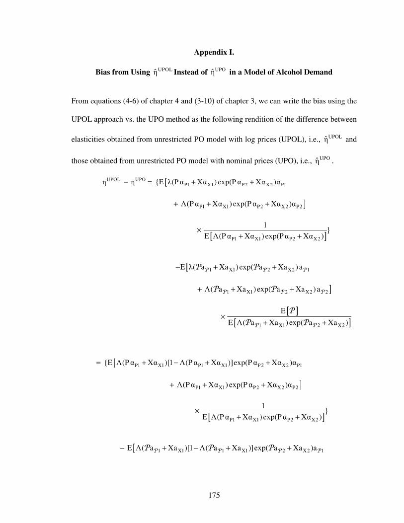
175

Appendix I.

Bias from Using UPOLη Instead of UPOη in a Model of Alcohol Demand

From equations (4-6) of chapter 4 and (3-10) of chapter 3, we can write the bias using the

UPOL approach vs. the UPO method as the following rendition of the difference between

elasticities obtained from unrestricted PO model with log prices (UPOL), i.e., UPOLη and

those obtained from unrestricted PO model with nominal prices (UPO), i.e., UPOη .

[UPOL UPOP1 X1 P2 X 2 P1η η E λ(P α Xα ) exp(P α Xα )α− = + +

]P1 X1 P2 X2 P2Λ(Pα Xα ) exp(Pα Xα )α+ + +

[ ]P1 X1 P2 X2

1

E Λ(Pα Xα ) exp(Pα Xα )×

+ +

[ 1 X1 2 X2 1E λ( a Xa ) exp( a Xa )a− + +P P PP P

]1 X1 2 X2 2Λ( a Xa )exp( a Xa )a+ + +P P PP P

[ ]

[ ]1 X1 2 X2

E

E Λ( a Xa ) exp( a Xa )×

+ +P P

P

P P

[ P1 X1 P1 X1 P2 X2 P1E Λ(Pα Xα )[1 Λ(Pα Xα )]exp(Pα Xα )α= + − + +

]P1 X1 P2 X2 P2Λ(Pα Xα ) exp(Pα Xα )α+ + +

[ ]P1 X1 P2 X2

1

E Λ(Pα Xα ) exp(Pα Xα )×

+ +

[ 1 X1 1 X1 2 X2 1E Λ( a Xa )[1 Λ( a Xa )]exp( a Xa )a− + − + +P P P PP P P

176

]1 X1 2 X2 2Λ( a Xa ) exp( a Xa )a+ + +P P PP P

[ ]

[ ]1 X1 2 X2

E

E Λ( a Xa ) exp( a Xa )×

+ +P P

P

P P. (I-1)

If we define

1 2v E[Λ(Wa )exp(Wa )]≡

21 2u E[Λ(W a ) exp(W a )]≡

[ ]m E=P P

1 2ν E[Λ(W α ) exp(W α )]≡

and

21 2ω E[Λ(W α ) exp(W α )]≡

where i i iW [P X ]=

denotes the observation on W [P X]=

for the ith individual in the

sample (i = 1, ..., n), with P expressed as log of alcohol price, and

i i iW [ X ]= P denotes the observation on W [ X]= P for the ith individual in

the sample (i = 1, ..., n), P with expressed as nominal price of alcohol.

AL UPO 1P1 P2 [(v u) a va ]m[(ν ω)α να ]η η

ν v

− +− +− = − P P2 P

P1 P2 1

ω u1 α α 1 a a mν v

= − + − − +

P P2 P . (I-2)

177

Appendix J.

Asymptotic Distribution (and Standard Error) of UPOL UPOˆ ˆη η−

In Appendix I we showed that

UPOL UPOP1 P2 1 2

ω uη η 1 α α 1 a a m

ν v

− = − + − − +

P P P

where

1 2ν E[Λ(Wα )exp(Wα )]≡

21 2ω E[Λ(W α ) exp(W α )]≡

1 2v E[Λ(Wa )exp(Wa )]≡

21 2u E[Λ(Wa ) exp(Wa )]≡

[ ]W P X=

[ ]W X=

P

and

[ ]m E≡P P

Using the corresponding consistent estimators for ω, ν, v and ω say

n

ii 1

1ˆ ˆω Ω(α, W )n=

∑=

n

ii 1

1ˆν = (α, W )

n=∑

V

178

n

ii 1

1ˆv = V(a , W )

n=∑

n

ii 1

1ˆu U(a , W )

n=∑=

and

n

ii 1

1m

n=∑=P P

2

1 2Ω(α, W) Λ(W α ) exp(W α )=

1 2(α, W ) Λ (W α ) exp(W α )=

V

1 2V(a , W) Λ(W a )exp(W a )=

21 2U(a , W) Λ(Wa ) exp(Wa )=

1 2ˆ ˆ ˆα [α α ]'′ ′= (with 1 1 X1

ˆ ˆ ˆα = [α α ]′ ′P and 2 2 X 2

ˆ ˆ ˆα = [α α ]′ ′P

) is the consistent

estimate of the parameter vector 1 2α [α α ]'′ ′= (with 1 1 X1α = [α α ]′ ′P and

2 2 X2α = [α α ]′ ′P ) [the parameters of equation (4-6)] obtained via the

two-part protocol culminating in (4-4) using the nominal prices of alcohol

1 2ˆ ˆ ˆa [a a ]'′ ′= (with 1 1 X1

ˆ ˆ ˆa = [a a ]′ ′P and 2 2 X2

ˆ ˆ ˆa = [a a ]′ ′P ) is the consistent

estimate of the parameter vector 1 2a [a a ]'′ ′= (with 1 1 X1a = [a a ]′ ′P and

2 2 X2a = [a a ])′ ′P ) [the parameters of equations (3-6) and (3-7),

respectively] obtained via the unrestricted two-part protocol culminating

in (3-8) using the log prices of alcohol

and i i iW [P X ]= denotes the observation on W [P X]= for the ith individual in the

sample

179

(i = 1, ..., n), and i i iW [ X ]=

P denotes the observation on W [ X]=

P for the ith

individual in the sample (i = 1, ..., n).

Let

P1 P2 1 2ˆ ˆˆ ˆ ˆ ˆˆ ˆ ˆτ = [α α a a ω ν u v m ]′

P P P

and

P1 P2 1 2τ = [α α a a ω ν u v m ]′ P P P , where ˆplim[τ] = τ .

If we could show that

1 d2ˆ ˆAVAR(τ) n (τ τ) N(0, I)

−

− →

where the formulation of ˆAVAR(τ) is known, then we could apply the δ-method to

obtain the asymptotic variance of UPOL UPOˆ ˆη η− as

UPOL UPOˆ ˆ ˆavar(η η ) c(τ) AVAR(τ) c(τ) '− =

180

where P1

2P1

1

21

1 2

ω 1

ν

1

u m 1

v

m

c(τ) α / ν

α ω / ν

m a / ν

m a u/ ν

u1 a a

v

′ −

− −

− = − −

− − −

P

P

P P

P P

P P

.

Moreover, if we have a consistent estimator for ˆAVAR(τ) , say AVAR(τ) [i.e.

ˆp lim AVAR (τ) AVAR (τ) =

], then we could consistently estimate

UPOL UPOˆ ˆavar(η η )− as

UPOL UPOˆ ˆ ˆ ˆ ˆavar(η η ) c(τ) AVAR(τ) c(τ) '− = . (J-1)

We focus, therefore, on finding the asymptotic distribution of τ and, in particular, the

formulation of its asymptotic covariance matrix.

First note that we can write τ as

τ Ξ θ= (J-2)

where θ = [δ γ ]′ ′ ′ , 1 2 1 2δ [α α a a ]'′ ′ ′ ′= , γ [ω ν u ν m ]′ = P (recall,

1 P1 X1α = [α α ]′ ′ , 2 P2 X2α = [α α ]′ ′ , 1 1 X1ˆ ˆ ˆa = [a a ]′ ′

P , and 2 2 X2ˆ ˆ ˆa = [a a ]′ ′

P ).

181

P1

P2

1

2

α

α

a

a

5,4K 5

Ξ

0 I

− − − − − − − − − − − − − − − −

= − − − − − − − − − − − − − − − −

P

P

a is the unit row vector with the value “1” in the element position corresponding to the

element position of a in the vector θ, b,c0 is the matrix of zeros whose row and column

dimensions are b and c, respectively, dI is the identity matrix of order d, and K is the

column dimension of W. For future reference, let’s set the following vector/matrix

dimensions:

1α is K×1

2α is K×1

1a is K×1

2a is K×1

W is 1×K

W

is 1×K

τ is 9×1

c(τ) is 1×9

δ is 4K×1

182

γ is 5×1

θ is (4K+5)×1

Ξ is 9×(4K+5)

P1 P2 1 2α α a a= = = =

P P 1×(4K+5)

Clearly then

ˆˆAVAR(τ) Ξ AVAR(θ) Ξ′= (J-3)

where θ is the estimator of θ obtained from the following two-stage protocol.

First Stage

Consistently estimate δ via the following optimization estimator

n

1 ii 1

δ

q (δ, S )δ = arg max

n=∑

(J-4)

where

1 i 11 1 i 12 2 i 13 1 i 14 2 iq (δ, S ) q (α , S ) q (α , S ) q (a , S ) q (a , S )= + + +

11 1 i i i 1 i i 1q (α , S ) I(A 0) ln[Λ(W α )] [1 I(A 0)] ln[1 Λ(W α )]= > + − > −

( )( )2

12 2 i i i i 2q (α , S ) I(A 0) A exp W α= − > −

13 1 i i i 1 i i 1q (a , S ) I(A 0) ln[Λ(W a )] [1 I(A 0)] ln[1 Λ(W a )]= > + − > −

( )( )2

14 2 i i i i 2q (a , S ) I(A 0) A exp W a= − > −

i i i iS [A X P ]= and i i i iS [A X ]=

P

183

1 22 1 2δ [α α a a ]'′ ′ ′ ′= , 1 P1 X1α = [α α ]′ ′ , 2 P2 X2α = [α α ]′ ′ , 1 1 X1a = [a a ]′ ′ P

,

2 2 X2a = [a a ]′ ′ P and 1 22 1 22

ˆ ˆ ˆ ˆ ˆδ [α α a a ] '′ ′ ′ ′=

Second Stage

Consistently estimate γ via the following optimization estimator

n

ii 1

γ

ˆq(δ, γ, S )γ = arg max

n=

∑

(J-5)

where

i a i b i c i d i e iˆ ˆ ˆ ˆ ˆ ˆq(δ, γ, S ) q (δ, ω, S ) q (δ, ν, S ) q (δ, u, S ) q (δ, v, S ) q (δ, m , S )= + + + +

P

2a i i

ˆ ˆq (δ, ω, S ) (Ω(α, W ) ω)= − −

2b i i

ˆ ˆq (δ, ν, S ) ( (α, W ) ν)= − − V

2c i i

ˆ ˆq (δ, u, S ) (U(a , W ) u)= − −

2d i i

ˆ ˆq (δ, v, S ) (V(a , W ) v)= − −

2e i i

ˆq (δ, m , S ) ( m )= − −

P PP

1 2 1 2ˆ ˆ ˆ ˆ ˆδ [α α a a ] '′ ′ ′ ′= is the first stage estimator of δ,

1 P1 X1ˆ ˆ ˆα = [α α ]′ ′ , 2 P2 X2

ˆ ˆ ˆα = [α α ]′ ′ , 1 1 X1ˆ ˆ ˆa = [a a ]′ ′

P and 2 2 X2

ˆ ˆ ˆa = [a a ]′ ′P .

Use 1q as shorthand notation for

1 11 1 12 2 13 1 14 2q (δ, S) q (α , S) q (α , S) + q (a , S) q (a , S) = + +

with

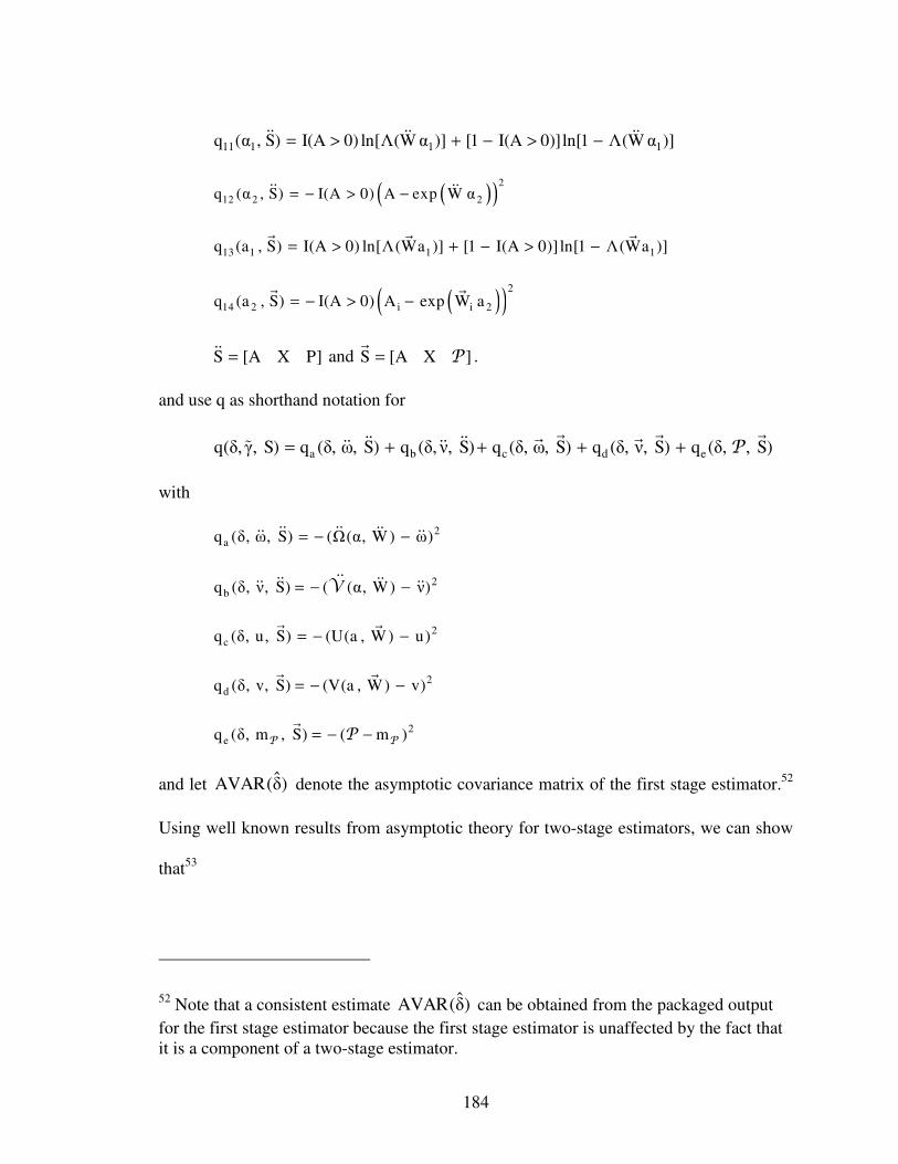
184

11 1 1 1q (α , S) I(A 0) ln[Λ(W α )] [1 I(A 0)]ln[1 Λ(W α )]= > + − > −

( )( )2

12 2 2q (α , S) I(A 0) A exp W α= − > −

13 1 1 1q (a , S) I(A 0) ln[Λ(Wa )] [1 I(A 0)] ln[1 Λ(Wa )]= > + − > −

( )( )2

14 2 i i 2q (a , S) I(A 0) A exp W a= − > −

S [A X P]= and S [A X ]=

P .

and use q as shorthand notation for

a b c d eq(δ,γ, S) q (δ, ω, S) q (δ, ν, S) q (δ, ω, S) q (δ, ν, S) q (δ, , S)= + + + + P

with

2aq (δ, ω, S) (Ω(α, W) ω)= − −

2bq (δ, ν, S) ( (α, W) ν)= − −

V

2cq (δ, u, S) (U(a , W) u)= − −

2dq (δ, v, S) (V(a , W) v)= − −

2eq (δ, m , S) ( m )= − −

P PP

and let ˆAVAR(δ) denote the asymptotic covariance matrix of the first stage estimator.52

Using well known results from asymptotic theory for two-stage estimators, we can show

that53

52 Note that a consistent estimate ˆAVAR(δ) can be obtained from the packaged output

for the first stage estimator because the first stage estimator is unaffected by the fact that it is a component of a two-stage estimator.

185

1 d2ˆ ˆAVAR(θ) n (θ θ) N(0, I)

−

− → (J-6)

where ˆˆ ˆθ = [δ γ ]′ ′ ′ , ˆplim(θ) = θ

11 12

12 22

D D

D DˆAVAR(θ)

= ′

(J-7)

11ˆAVAD R(δ)= (J-8)

4K×4K

[ ]12 δδ 1 δ 1 γ γγ

11E ED q q ' q E q

−−= ∇ ∇ ∇ ∇

[ ] [ ] [ ]δδ 1 δ 1 δ 1 δδ 1 γ

1

γ

1

δ

1

γE q q ' q q q qE E E E−− −

∇ ∇′ − ∇ ∇ ∇ ∇ (J-9)

22 γγ γδ γ

1

δˆˆAVAR (γ) E E AVD q q qAR (δ)E '

− = = ∇ ∇ ∇

[ ]γ δ 1 δδ 1 γδ

1q ' q qE E E q

−∇ ∇

′ − ∇ ∇

[ ]γδ δδ 1 γ δ 1 γ

1

γ

1q q q ' q qE E E ' E

−− − ∇ ∇∇ ∇ ∇

1 1

γγ γ γ γγq q ' q qE E E− −

∇ ∇ ∇ + ∇ . (J-10)

Fortunately, (J-9) and (J-10) can be simplified in a number of ways. First note that we

can write

γ δ 1 γ δ 1q ' q q 'E W]E |E [ q∇ = ∇ ∇ ∇

53Discussions of asymptotic theory for two-stage optimization estimators can be found in Newey & McFadden (1994), White (1994, Chapter 6), and Wooldridge (2010, Chapter 12).

186

but

δ 1 δ 11 δ 12 δ 13 δ 14q = q q q q∇ ∇ + ∇ + ∇ + ∇

with

1δ 11 αq [ ln f (I(A 0) | W) 0 0 0]∇ = ∇ >

( )( ) ( )δ 12 2 2I(A 0) A exp W α exq 0 2 0 0p W α W ∇ =

> −

1δ 13 aq 0 0 ln f (I(A 0) | W) 0 ∇ = ∇ >

( )( ) ( )2δ 214 I(A 0) A exq 0 0 p Wa 0 2 exp Wa W> ∇ = −

where

I(A 0) [1 I(A 0)]1 1Λ(W α ) [1f (I( Λ(A 0) W) W α )]| > − >=> − .

I(A 0) [1 I(A 0)]1 1Λ(Wa ) [1 Λ(f (I( WaA ) | W) )]0 > − >> = −

.

Therefore

( )( ) ( )

( )( ) ( )

1

1

α

δ 1

a

2 2

2 2

E[ ln f (I(A 0) | W)]

2E

E[ q | W]E[ ln f (I(A 0) | W)]

2E

I(A 0) A exp W α exp W α | W W

I(A 0) A exp Wa exp Wa | W W

′ ∇ >

∇ =

∇ >

> −

−

>

= [ 0 0 0 0]

because 1α

E[ ln f (I(A 0) | W )] 0∇ > = and 1aE[ ln f (I(A 0) | W)] 0∇ > =

[see (13.20) on

p. 477 of Wooldridge (2010)], ( )( ) ( )2 2I(A 0) A exp W α e W 0WE xp α |> =

− and

( )( ) ( )2 2I(A 0) A exp Wa exp Wa | WE 0 =>−

, by design. Finally, then we get

187

γ δ 1q ' qE 0 = ∇ ∇

so

[ ] [ ] [ ]12 δδ 1 δ 1 δ 1 δδ 1 γδ γγ

11 1E E E ED q q ' q q q qE

−− − ′ − = ∇ ∇ ∇ ∇ ∇ ∇ (J-11)

4K×4K 4K×4K 4K×4K 4K×5 5×5 4K×5 and

22 γγ γδ γδ γγ

1 1ˆˆAVAR(γ) E E AVAR(δ) E 'ED q q q q− −

= ∇ ∇ ∇ = ∇

5×5 5×4K 4K×4K 4K×5 5×5

1 1

γγ γ γ γγq q ' q qE E E− −

∇ ∇ ∇ + ∇ . (J-12)

5×5 5×5 5×5 5×5 so

11 1

(4K 5) (4K

2

12 25) 2

D D

4K 4K 4K 5

D D

5 4K

ˆAVAR(

5 5

θ)+ × +

× × = ′

× ×

.

Let’s consider each of the individual components of (J-6) and (J-7) in turn.

δ1

δ 1qE[ ]−−−−∇∇∇∇

4K×4K

Written out explicitly we have

1 1

2 2

1 1

2 2

α α 11

1α α 12

δδ 1 1a a 13

a 1

1

1

1a 4

E[ q ] 0 0 0

0 E[ q ] 0 0q ]

0 0 E[ q ] 0

0 0 0 E[

[

]

E

q

−

−

−

−

−

∇ ∇ ∇ = ∇ ∇

.

(J-13)

188

Now

1 1

11 1α α 1E ˆAV[ ] )q AR(α− = −∇ (J-14)

= the negative of the asymptotic covariance matrix for first

stage, first part, logit estimation in the two-stage estimation

protocol for θ. We get an estimate of this directly from the Stata

output.

A consistent estimator of 1 1α α 11

1E[ q ]−∇ is

1 1

1α 1 1α 1

ˆ ˆnAVAR *(αE q ] )[ − = −∇ (J-15)

where 1ˆAVAR * (α ) is the estimated variance-covariance matrix output by the Stata logit

procedure. Also

( )( ) ( )2α 2 212 I(A 0) A exp Wα expq 2 Wα W>∇ = −

and

( )( ) ( ) ( )2 2α α 2 212 2I(A 0) A exp Wα exp Wα exp Wα W Wq 2 ′> − −

∇

= .

Therefore

( )( ) ( ) ( )2 2α 2α 1 2 22 I(A 0) A exp Wα exp Wα expE[ q ] 2E Wα W W ′> − − ∇ =

.

(J-16)

A consistent estimator of 2 2

1α α 12E[ q ]−∇ is

189

( )( ) ( ) ( ) 2 2

1n

1α 12 1α i i i 2 i 2 i 2 i i

i 1

I(A 0) A expE[ q ] W α exp W α exp W α Wn W2−

−

=

∑ ′> − −

∇ =

(J-17)

where 2α is the first stage, second part, estimator of 2α , and 1n is the size of the

subsample for whom I(A 0) 1> = .

Similarly,

1 1

11 1a a 3E ˆAV[ ] )q AR(a− = −∇ (J-18)

= the negative of the asymptotic covariance matrix for first

stage, first part, logit estimation in the two-stage estimation

protocol for θ. We get an estimate of this directly from the Stata

output.

A consistent estimator of 1 1a a 13

1E[ q ]−∇ is

1 1

1a 1 1a 3

ˆ ˆnAVAR *(aE q ] )[ − = −∇ (J-19)

where 1ˆAVAR * (a ) is the estimated variance-covariance matrix output by the Stata logit

procedure. Also

( )( ) ( )2 2a 213 I(A 0) A eq xp Wa W W2 exp a∇ = > −

and

( )( ) ( ) ( )2 2 2 2 2a a 14 I(A 0) A exp Wa exp Waq exp Wa W W2 ′> − −∇

=

.

Therefore

190

( )( ) ( ) ( )2 2a a 14 2 2 2I(A 0) A exp Wa exp WaE[ exp WE aq W2 W] ′> − −

∇ =

.

(J-20)

A consistent estimator of 2 2

1a a 14E[ q ]−∇ is

( )( ) ( ) ( ) 2 2 i i i 2 i 2

1n

1a a 14 1

i 1i 2 i iI(A 0) A exp W a exp W a exp W a WE[ q ] n 2 W

−−

=

∑ ′> − −

∇ =

(J-21)

where 2a is the first stage, second part, estimator of 2a , and 1n is the size of the

subsample for whom I(A 0) 1> = .

so

1 1

2 2

1 1

2 2

α α 11

1α α 12

δδ 1 1a a 13

1

a a

1

114

E

EE[

ˆ

[ q ] 0 0 0

0 [ q ] 0 0q ]

0 0 [ q ] 0

0 0 0 [

E

qE ]

−

−

−

−

−

∇ ∇ ∇ = ∇ ∇

.

(J-22)

δ 1 δ 1q ' qE ∇ ∇∇ ∇∇ ∇∇ ∇

4K×4K Written out explicitly we have

191

[ ]

1 1 1 1

1 2 1 2

2 2 2 2

1 2 1 2

1

1

α 11 α 11 α 11 α 11

α 11 α 12 a 13 a 14

α 12 α 12 α 12 α 12

α 11 α 12 a 13 a 14

δ 1 δ 1

a 13

α 1

q ' q ' q ' q '

q q q q

q ' q ' q ' q '

q q q qq

E E E E

E E E

' qq

E

'

q

E

E

∇ ∇ ∇ ∇

∇ ∇ ∇ ∇

∇

∇ ∇ ∇

∇ ∇ ∇ ∇∇ ∇

∇

∇

=

1 1 1

2 1 2

2 2 2 2

1 2 1 2

a 13 a 13 a 13

1 α 12 a 13 a 14

a 14 a 14 a 14 a 14

α 11 α 12 a 13 a 14

q ' q ' q '

q q q

q ' q ' q ' q '

q q

E E E

E E Eq q

E

∇ ∇ ∇ ∇ ∇ ∇ ∇ ∇ ∇ ∇

∇ ∇ ∇ ∇

.

(J-23)

Because the first stage, first part, estimator of 1α is MLE we can write

[ ]1 1 1 1α 11 α 11 α α

1

111ˆE[ q ' q ] E[ AVARq ] )α(

−∇ ∇ − ∇ ==

= the inverse of the asymptotic covariance matrix for first stage,

first part, logit estimation in the two-stage estimation

protocol for θ. We get an estimate of this directly from the

Stata output.

A consistent estimator of 1 1α 11 α 11E[ q ' q ]∇ ∇ is

1 1α 11 α 1

1

1 1

1ˆAVARE[ q ' *(α )

nq ]

− =

∇ ∇ (J-24)

where 1ˆAVAR * (α ) is the estimated variance-covariance matrix output by the Stata logit

procedure.

192

Similarly, because the first stage, first part, estimator of 1a is also MLE we can write

[ ]1 1 1 1a 13 a 13 a a

1

113E[ q ' q ] E[ ˆAVARq ] (a )−

∇ ∇ − ∇ ==

= the inverse of the asymptotic covariance matrix for first stage,

first part, logit estimation in the two-stage estimation

protocol for θ. We get an estimate of this directly from the

Stata output.

A consistent estimator of 1 1a 13 a 13E[ q ' q ]∇ ∇ is

1 1a 13 a 1

1

3 1

1ˆAVARE[ q ' *(a )

nq ]

− =

∇ ∇ (J-25)

where 1ˆAVAR * (a ) is the estimated variance-covariance matrix output by the Stata logit

procedure.

The remainder of the block elements follow from

1 1 1 1α 11 αq ln f (I(A 0) | W) I(A 0)[1 Λ( I(W α )] [1 W α ))]Λ( WA 0∇ = ∇ > = > − > − −

(J-26)

( )( ) ( )2 2α 212 I(A 0) A exp Wα expq 2 Wα W>∇ = − . (J-27)

1 1a 13 a 1 1q ln f (I(A 0) | W) I(A W0)[1 Λ( I(A 0a )] [1 Wa ) W)]Λ(∇ = ∇ > = > − − − >

(J-28)

( )( ) ( )2 2a 214 I(A 0) A eq xp Wa W W2 exp a∇ = > −

. (J-29)

193

where the formulation of 1α 11q∇ and

1a 13q∇ comes from equation (16.4.8) on p. 350 of

Fomby et al. (1984) and Λ( ) denotes the logistic cdf. The remaining required consistent

matrix estimators are

1 2 1 2

n

α 11 α 12 α 11i α 12ii 11

1ˆ ˆ ˆE[ q ' q ] q ' qn =

∑∇ ∇ = ∇ ∇ (J-30)

2 2 2 2

n

α 12 α 12 α 12i α 12ii 11

1ˆ ˆ ˆE[ q ' q ] q ' qn =

∑∇ ∇ = ∇ ∇ (J-31)

1 1 1 1

n

α 11 a 13 α 11i a 13ii 11

1ˆ ˆ ˆE[ q ' q ] q ' qn =

∑∇ ∇ = ∇ ∇ (J-32)

2 1 2 1

n

α 12 a 13 α 12i a 13ii 11

1ˆ ˆ ˆE[ q ' q ] q ' qn =

∑∇ ∇ = ∇ ∇ (J-33)

1 2 1 2

n

α 11 a 14 α 11i a 14ii 11

1ˆ ˆ ˆE[ q ' q ] q ' qn =

∑∇ ∇ = ∇ ∇ (J-34)

2 2 2 2

n

α 12 a 14 α 12i a 14ii 11

1ˆ ˆ ˆE[ q ' q ] q ' qn =

∑∇ ∇ = ∇ ∇ (J-35)

1 2 1 2

n

a 13 a 14 a 13i a 14ii 11

1ˆ ˆ ˆE[ q ' q ] q ' qn =

∑∇ ∇ = ∇ ∇ (J-36)

2 2 2 2

n

a 14 a 14 a 14i a 14ii 11

1ˆ ˆ ˆE[ q ' q ] q ' qn =

∑∇ ∇ = ∇ ∇ (J-37)

where

1α 11i i i i i i1 1

ˆW α )] [1 W )ˆ ˆq I(A 0)[1 Λ( I(A 0)]Λ( α W − −∇ = > − > (J-38)

( )( ) ( )2α 12i i i 2 i 2i iˆ ˆI( 0) A exp W α exq α2 A p W W∇ > −= (J-39)

194

1a 13i i i i i 1 i1W )]ˆ ˆ ˆq I(A 0)[1 Λ( a I(A 0[1 W ) W)]Λ( a∇ = − − > − >

(J-40)

and

( )( ) ( )2 i i 2 ia 14i i i2

ˆ ˆI( 0) A exp W a exp Wq 2 a WA > −∇ =

(J-41)

so

[ ]

1 1 1 1

1 2 1 2

2 2 2 2

1 2 1 2

α 11 α 11 α 11 α 11

α 11 α 12 a 13 a 14

α 12 α 12 α 12 α 12

α 11 α 12 a 13 a 14

δ 1 δ 1

a

q ' q ' q ' q '

q q q q

q ' q ' q ' q '

q q q qq ' q

ˆ ˆ ˆ ˆE E E E

ˆ ˆ ˆ ˆE E E E

E

E

∇ ∇ ∇ ∇

∇ ∇ ∇ ∇

∇ ∇ ∇

∇

∇ ∇ ∇ ∇=∇ ∇

∇1 1 1 1

1 2 1 2

2 2 2 2

1 2 1 2

13 a 13 a 13 a 13

α 11 α 12 a 13 a 14

a 14 a 14 a 14 a 14

α 11 α 12 a 13 a 14

q ' q ' q ' q '

q q q q

q ' q ' q ' q '

q

ˆ ˆ ˆE E E

ˆ ˆ ˆ ˆE E E Eq q q

∇ ∇ ∇ ∇ ∇ ∇ ∇ ∇ ∇ ∇ ∇

∇

∇ ∇ ∇

.

(J-42)

γδqE ∇∇∇∇

5×4K Written out explicitly we have

ω a

ν b

u cγ

v d

m e

( q 0 0 0 0)

(0 q + 0 + 0 + 0)

(0 + 0 q + 0 + 0)q =

(0 + 0 + 0 q + 0)

(0 + 0 + 0 + 0 q )

′∇ + + + +

+∇ +∇∇

+∇ +∇

P

ω a ν b u c v d m e[ q q q q q ] ∇ ∇ ∇ ∇ ∇= P

195

( ) ( ) ( ) ( ) ( )2 Ω(α, W) ω (α, W) ν U(a, W) ω V(a, W) ν m = − − − − −

PV P

(J-43) and

1 2 1 2

1 2 1 2

1 2 1 2

1 2 1 2

1 2 1

ωα a ωα a ωa a ωa a

να b να b νa b va b

uα c uα c ua c ua cγδ

vα d vα d va d va d

m α e m α e m a e

E[ q ] E[ q ] E[ q ] E[ q ]

E[ q ] E[ q ] E[ q ] E[ q ]

E[ q ] E[ q ] E[ q ] E[ q ]E[ q] =

E[ q ] E[ q ] E[ q ] E[ q ]

E[ q ] E[ q ] E[ q ] E[

∇ ∇ ∇ ∇

∇ ∇ ∇ ∇

∇ ∇ ∇ ∇∇

∇ ∇ ∇ ∇

∇ ∇ ∇

P P P 2m a eq ]

∇ P

1 2 1 2

1 2 1 2

1 2 1 2

1 2 1 2

α α a a

α α a a

α α a a

α α a a

E[ Ω] E[ Ω] E[ Ω] E[ Ω]

E[ ] E[ ] E[ ] E[ ]

= 2 E[ U] E[ U] E[ U] E[ U]

E[ V] E[ V] E[ V] E[ V]

0 0 0 0

∇ ∇ ∇ ∇ ∇ ∇ ∇ ∇

∇ ∇ ∇ ∇

∇ ∇ ∇ ∇

V V V V

(J-44)

where

1 1α 1 22Λ(W )λ(W ) exp(W )Ω α Wα α∇ = (J-45)

2

2α 1 2Λ(W α ) exp(W WΩ α )=∇ (J-46)

1 1α 2λ(W α ) exp(W α ) W∇ = V (J-47)

2 1α 2Λ(W α ) exp(W α ) W∇ = V (J-48)

1 1a 1 22Λ(Wa )λ(Wa )exp(U Wa ) W=∇

(J-49)

2

21 2a Λ(Wa ) exp( aU W )W=∇

(J-50)

1 1a 2λ(Wa )exp( aV W ) W∇ =

(J-51)

2 1a 2Λ(Wa )exp( aV W ) W∇ =

(J-52)

196

and

ωa a ωa b va a va b uα c uα d vα c vα d m δ eq q q q q q q q q 0∇ = ∇ = ∇ = ∇ = ∇ = ∇ = ∇ = ∇ = ∇ = P.

(J-53)

Note that

aΛ(a) λ(a) Λ(a)[1 Λ(a)]∇ = = −

aλ(a) λ(a)[1 2Λ(a)]∇ = − .

The requisite consistent matrix estimators are

1 1

n

α α ii 1

E[ Ω] ==∑∇ ∇ Ω (J-54)

2 2

n

α α ii 1

E[ Ω] = Ω=∑∇ ∇ (J-55)

1 1

n

α α ii 1

E[ ] ==∑∇ ∇

V V (J-56)

2 2

n

α α ii 1

E[ ] ==∑∇ ∇

V V (J-57)

1 1

n

a a ii 1

E[ U] = U=∑∇ ∇ (J-58)

2 2

n

a a ii 1

E[ U] = U=∑∇ ∇ (J-59)

1 1

n

a a ii 1

E[ V] = V=∑∇ ∇ (J-60)

and

2 2

n

a a ii 1

E[ V] = V=∑∇ ∇ (J-61)

197

where

1 1 1i i 2α i ii2Λ(W )λˆ ˆ ˆΩ α α(W )exp(W ) Wα=∇ (J-62)

2

2α i ii 1 2Λ(W ) expˆ ( WˆΩ α αW )=∇ (J-63)

1α i i 2 ii 1λ(W ) exp(ˆ ˆ= α )αW W∇ V (J-64)

2α i i 2 ii 1Λ(W ) exp(ˆ ˆ= α )αW W∇ V (J-65)

1 1 1 2a i i i ii

2Λ(W )λ(W ) exp(W ) Wˆ ˆ ˆU a a a∇ =

(J-66)

2a i ii

21 2Λ(W ) exp(Wˆ a Wa )ˆU =∇

(J-67)

1 1 2a i i ii

λ(W ) exp(Wˆ ˆV = a a ) W∇

(J-68)

and

2 1 2a i i ii

Λ(W ) exp(Wˆ ˆV = a a ) W∇

(J-69)

so

1 2

1 2

1 2

1 2

α α

α α

γδ a a

a a

ˆ ˆE[ Ω] E[ Ω] 0 0

ˆ ˆE[ ] E[ ] 0 0

E[ q] = 2 ˆ ˆ0 0 E[ U] E[ U]

ˆ ˆ0 0 E[ V] E[ V]

0 0 0 0

∇ ∇ ∇ ∇

∇ ∇ ∇ ∇ ∇

V V

. (J-70)

γγ1E[ q]−−−−∇∇∇∇

5×5

198

[ ]

[ ]

[ ]

[ ]

1

1

1 1

ωω a

νν b

uu cγγ

vv d

1

1

m m e

E 0 0 0 0

0 E 0 0 0

0 0 E 0 0E

0 0 0 E 0

0 0 0 0 E

q

q

qq

q

q

−

−

− −

−

−

=

∇

∇

∇∇

∇

∇

P P

(J-71)

because ij kq 0∇ = where i, j ω, v, u, v, ; k= a, b,c,d, e am nd i j= ≠ P .

Now

ωω a νν b uu c vv d m m eq q q q q 2∇ = ∇ = ∇ = ∇ = ∇ = − P P

therefore

γ

1

γ

10 0 0 0

2

10 0 0 0

2

1E 0 0 0 0

2

10 0 0 0

2

10 0 0

q

02

−

− − = −

−

−

∇ . (J-72)

γ γq ' qE ∇ ∇∇ ∇∇ ∇∇ ∇

5×5

Given that

199

( ) ( ) ( ) ( ) ( )iγ 2 Ω(α, W) ω (α, W) ν U(a, W) u V(a, W) v m q ∇ = − − − − −

PV P .

(J-73)

we have

γ γq ' qE ∇ ∇ =

2i

(Ω(α, W) (Ω(α, W) (Ω(α, W) (Ω(α, W)

ω) ω) ω)(Ω(α, W) E ω)E E E E

(P m )ω) (U(a, W) (V(a, W)( (α, W)

u) v)ν)

(

E

4

− − − − −−

− −−

PV

2i

Ω(α, W) ( (α, W)( (α, W) ( (α, W)

ω) E ν)ν) ν)( (α, W)E E E

(P m )( (α, W) ν) (U(a, W) (V(a, W)

ν) u) v)

(Ω(

E

− −− − − −

− − −

P

VV V

V

V

2i

α, W) (U(a, W)(U(a, W)( (α, W)

ω) E u)u)(U(a, W)ν)E E E

(P m )(U(a, W) u) (V(a, W)(U(a, W)

u) v)u)

(Ω(α, W)

ω)E

( (α, W)

− −−− −−

− −−

−

−

P

V

V2

i

i

(U(a, W)( (α, W) (V(a, W)

u)ν) E v)(V(a, W)E E E

(P m )v)( (α, W)( (α, W)

ν) ν)ν)

(Ω(α, W) ( (α

E ω) E

(P m )

−− − −−

−−

− −

P

P

V

VV

V

i

i i i i

, W) (U(a, W) (V(a, W)

(P m )ν) E u) E v)E

(P m ) (P m ) (P m ) (P m )

−− − − − − − −

P

P P P P

.

(J-74)

200

The corresponding consistent estimator is

n n2

i i ii 1 i 1

n n2

γ γ i i ii 1 i 1

ˆ1 1ˆ ˆˆ ˆ ˆ(Ω ω) (Ω ω)( ν)n n

ˆ ˆ1 1ˆ ˆ ˆ ˆE 4 (Ωq ' ω)( ν) ( ν)n

q .n

= =

= =

∑ ∑

∑ ∑

− − −

= − − −

∇

∇

V

V V

(J-75)

Based on (J-8), (J-11) and (J-12) and using the two-stage estimator θ we can consistently

estimate (J-7) as

11 12

12 22

ˆ ˆD D

ˆ ˆD D

ˆAVAR(θ)

= ′

where

1

1 2

1

11

1 2

0 0 0

0 0 0D

0

ˆnAVAR *(α )

ˆn AVAR *(α )ˆAVAR(δ)ˆnAVAR *(a )

ˆn AVAR *(a

0

)

0

0 0 0

=

=

[ ]12 γγ δ 1 δ 1 γγ γδ γ

1 1

γ

1ˆ ˆ ˆ ˆ ˆE E E E ED q q ' q q q q− − −′ = ∇ ∇ ∇ ∇ ∇ ∇ −

22 γγ γδ

1 1

γδ γγˆˆ ˆ ˆ ˆˆAVAR (γ) E E AVAR (δ) E 'D q Eq q q

− − = ∇ ∇ ∇ = ∇

γγ γ γ γγ

1 1q q ' q qˆ ˆ ˆE E E

− −∇ ∇ ∇ + ∇

201

and using well known results from asymptotic theory for two-stage estimators, we can

show that54

1 1

1 2 2

1 1

1 1 2 2d

2

ˆn (α α )

ˆn (α α )

ˆn (a a )

ˆn (a a )

ˆ ˆAVAR(θ) N(0, I)n (ω ω)

ˆn (ν ν)

ˆn (u u)

ˆn (v v)

ˆn (m m )

−

−

−

−

− →− −

−

−

−

P P

. (J-76)

************************************************************************ ASIDE:

Notice that the “ n blow up” is a bit tricky here. It implements n for 1α , ω , ν and 1a

; but uses 1n for 2α and 2a . We had to do this because we had to use the correct

sample size (viz., 1n ) for a number of the components of AVAR(θ) [viz., those that

pertained to the estimation of 2ρ , and 2α ]; in particular (J-17), (J-21), (J-30) through (J-

37). For this reason we had to be explicit about the denominators in all of the averages

for the components of AVAR(θ) . This meant that in the construction of the requisite

54Discussions of asymptotic theory for two-stage optimization estimators can be found in Newey & McFadden (1994), White (1994, Chapter 6), and Wooldridge (2010, Chapter 12).

202

asymptotic t-stats we had to explicitly include the “blow-up” in the numerator (i.e., we

had to multiply by the square-root of the appropriate sample size). I refer to this as

“tricky” because one typically does not have to do this. In the usual asymptotic t-stat

construction the denominators of the averages (“n”) need not be included in the

construction of the asymptotic covariance matrix because it typically manifests as a

multiplicative factor and, after pulling the diagonal and taking the square root to get the

standard errors, this multiplicative n cancels with the “blow-up” factor in the

numerator. For example, the asymptotic t-stat of the OLS estimator is

( ) ( )

k k k k k k k k

1 1 12 22 kk kk

kk

ˆ ˆ ˆ ˆn (ρ ρ ) n (ρ ρ ) n (ρ ρ ) (ρ ρ )

ˆAVAR(ρ) ˆ ˆn σ σ1σ

n

− − −

− − − −= = =

′ ′ ′

XX XXXX

where

n is the sample size

kρ is the coefficient of the kth regressor in the linear regression

kρ is its OLS estimator

2σ is the regression error variance estimator

X is the matrix of regressors

and kk′XX is the kth diagonal element of ′XX . Note how the “ n s” simply cancel.

Note also that what we typically refer to as the “asymptotic standard error” can actually

be written as the square root of the diagonal element of the consistent estimator of the

asymptotic covariance matrix divided by n; in other words

203

asy std err = AVAR(ρ)

n.

***********************************************************************

Now back to the issue at hand. Moreover

P1 P1

1 P2 P2

1 1

1 2 21 d2

ˆn(α α )

ˆn (α α )

ˆn(a a )

ˆn (a a )

ˆˆAVAR(τ) n N(0, I)n(ω ω)

ˆn (ν ν)

ˆn(u u)

ˆn (v v)

ˆn(m m )

−

−

−

−

− →− −

−

−

−

P P

P P

P P

. (J-77)

where

ˆAVAR(τ) ΞAVAR(θ) Ξ '= (J-78)

and τ and Ξ are defined as in (J-2). Now combining (J-1) with (J-77) and (J-78) we get

( ) ( )

1d

UPOL UPO UPOL UPO UPOL UPO2ˆ ˆ ˆ ˆavar(η η ) n η η η η N(0, I)−

− − − − →

(J-79)

where

UPOL UPOˆ ˆ ˆ ˆ ˆavar(η η ) c(τ) AVAR(τ) c(τ) '− =

and

204

P1

2P1

1

21

1 2

ω 1

ν

1

u m 1

v

m

c(τ) α / ν

α ω / ν

m a / ν

m a u/ ν

u1 a a

v

′ −

− −

− = − −

− − −

P

P

P P

P P

P P

.

205

REFERENCES

Alcohol Justice. (2014). Methodology and Faq. Alcohol Tax/Fee Revenue Calculator Angrist, J. D., and Pischke, J. S. (2009). Mostly Harmless Econometrics: An Empiricist's

Companion, Princeton university press. Ayyagari, P., Deb, P., Fletcher, J., Gallo, W., and Sindelar, J. L. (2013). Understanding

Heterogeneity in Price Elasticities in the Demand for Alcohol for Older Individuals. Health Economics, 22(1), 89-105.

Beer Institute. (2013). Brewers Almanac. Available on

http://www.beerinstitute.org/br/beer-statistics/brewers-almanac, retrieved on May 27, 2015.

Blake, D., and Nied, A. (1997). The Demand for Alcohol in the United Kingdom.

Applied Economics, 29(12), 1655-1672. Byrnes, J., Shakeshaft, A., Petrie, D., and Doran, C. (2013). Can Harms Associated with

High‐Intensity Drinking Be Reduced by Increasing the Price of Alcohol?. Drug

and Alcohol Review, 32(1), 27-30. C2ER-COLI. (2015). Cost of Living Index. Council of Community and Econoic Research

Cameron, L., and Williams, J. (2001). Cannabis, Alcohol and Cigarettes: Substitures or

Complements?. The Economic Record, 77(236), 19-34. Chaloupka, F.J., and Laixuthai, A. (1997). Do Youths Substitute Alcohol and Marijuana?

Some Econometric Evidence. Eastern Economic Journal, 23(3), 253-275. Chaloupka, F. J., Saffer, H., and Grossman, M. (1993). Alcohol-Control Policies and

Motor-Vehicle Fatalities. The Journal of Legal Studies, 22(1), 161-186. Chesson, H., Harrison, P., and Kassler, W. J. (2000). Sex under the Influence: The Effect

of Alcohol Policy on Sexually Transmitted Disease Rates in the United States*. The Journal of Law and Economics, 43(1), 215-238.

Coate, D., and Grossman, M. (1988). Effects of Alcoholic Beverage Prices and Legal

Drinking Ages on Youth Alcohol Use. Journal of Law and Economics, 31(1). Congressional Budget Office. (1990). The Distributional Effects of Increases in Federal

Taxes on Tobacco, Alcoholic Beverages, and Motor Fuels. Federal Taxation of

Tobacco, Alcohol Beverages , and Motor Fuels, Chapter 5, 69-70

206

Congressional Budget Office. (2013). Option#32 - Options for Reducing the Deficit: 2014 to 2023. Available https://www.cbo.gov/budget-options/2013/44854, retrieved on May 27, 2015

Congressional Budget Office. (2014). Option#71 - Options for Reducing the Deficit:

2015 to 2024. Available https://www.cbo.gov/budget-options/2014/49653, retrieved on May 27, 2015

Cook, P. J., and Durrance, C. P. (2013). The Virtuous Tax: Lifesaving and Crime-

Prevention Effects of the 1991 Federal Alcohol-Tax Increase. Journal of Health

Economics, 32(1), 261-267. Cook, P. J., and Moore, M. J. (1993). Economic Perspectives on Reducing Alcohol-

Related Violence. Alcohol and Interpersonal Violence: Fostering

Multidisciplinary Perspectives, 24, 193-211. Cook, P. J., and Moore, M. J. (2002). The Economics of Alcohol Abuse and Alcohol-

Control Policies. Health Affairs, 21(2), 120-133. Elder, R. W., Lawrence, B., Ferguson, A., Naimi, T. S., Brewer, R. D., Chattopadhyay, S.

K., . . . Fielding, J. E. (2010). The Effectiveness of Tax Policy Interventions for Reducing Excessive Alcohol Consumption and Related Harms. American Journal

of Preventive Medicine, 38(2), 217-229. Farrell, S., Manning, W. G., and Finch, M. D. (2003). Alcohol Dependence and the Price

of Alcoholic Beverages. Journal of Health Economics, 22(1), 117-147. Fomby, T., Hill, R.C., and S. Johnson (1984): Advanced Econometrics, Springer-

Verlag.Goel, R. K., & Morey, M. J. (1995). “The interdependence of cigarette and liquor demand.” Southern Economic Journal, 451-459.

Gallet, C. A. (2007). The Demand for Alcohol: A Meta‐Analysis of Elasticities*. Australian Journal of Agricultural and Resource Economics, 51(2), 121-135.

Goel, R. K., and Morey, M. J. (1995). The Interdependence of Cigarette and Liquor Demand. Southern Economic Journal, 62(2), 451-459.

Grossman, M., Chaloupka, F. J., Saffer, H., and Laixuthai, A. (1994). Effects of Alcohol

Price Policy on Youth: A Summary of Economic Research. Journal of Research

on Adolescence, 4(2), 347-364. Kenkel, D. S. (1993). Drinking, Driving, and Deterrence: The Effectiveness and Social

Costs of Alternative Policies. Journal of Law and Economics, 36(2), 877-913. Kenkel, D. S. (1996). New Estimates of the Optimal Tax on Alcohol. Economic Inquiry,

34(2), 296-319.

207

Kenkel, D. S. (2005). Are Alcohol Tax Hikes Fully Passed through to Prices? Evidence

from Alaska. American Economic Review, 95(2), 273-277. Laixuthai, A., and Chaloupka, F. J. (1993). Youth Alcohol Use and Public Policy.

Contemporary Economic Policy, 11(4), 70-81. Lee, B., and Tremblay, V. J. (1992). Advertising and the Us Market Demand for Beer.

Applied Economics, 24(1), 69-76. Leung, S. F., and Phelps, C. E. (1993). My Kingdom for a Drink...? A Review of

Estimates of the Price Sensitivity of Demand for Alcoholic Beverages. Economics

and the Prevention of Alcohol-Related Problems. NIAAA Research

Monograph(25), 1-32. Levy, D., and Sheflin, N. (1983). New Evidence on Controlling Alcohol Use through

Price. Journal of Studies on Alcohol and Drugs, 44(06), 929. Levy, D., and Sheflin, N. (1985). The Demand for Alcoholic Beverages: An Aggregate

Time-Series Analysis. Journal of Public Policy & Marketing, 4, 47-54. Manning, W. G., Blumberg, L., and Moulton, L. H. (1995). The Demand for Alcohol:

The Differential Response to Price. Journal of Health Economics, 14(2), 123-148. Manning, W. G., Keeler, E. B., Newhouse, J. P., Sloss, E. M., and Wasserman, J. (1989).

The Taxes of Sin: Do Smokers and Drinkers Pay Their Way?. JAMA, 261(11), 1604-1609.

Markowitz, S., and Grossman, M. (1998). Alcohol Regulation and Domestic Violence

Towards Children. Contemporary Economic Policy, 16(3), 309-320. Markowitz, S., and Grossman, M. (2000). The Effects of Beer Taxes on Physical Child

Abuse. Journal of Health Economics, 19(2), 271-282. Mullahy, J., and Sindelar, J. L. (1994). Do Drinkers Know When to Say When? An

Empirical Analysis of Drunk Driving. Economic Inquiry, 32(3), 383-394. Mullahy, J., and Sindelar, J. (1996). Employment, Unemployment, and Problem

Drinking. Journal of Health Economics, 15(4), 409-434. Mullahy, J. (1998). Much Ado About Two: Reconsidering Retransformation and the

Two-Part Model in Health Econometrics. Journal of Health Economics, 17(3), 247-281.

Nelson, J. P. (1990). State Monopolies and Alcoholic Beverage Consumption. Journal of

Regulatory Economics, 2(1), 83-98.

208

Nelson, J. P. (2014). Estimating the Price Elasticity of Beer: Meta-Analysis of Data with

Heterogeneity, Dependence, and Publication Bias. Journal of Health Economics,

33, 180-187. Newey, W.K. and McFadden, D. (1994): Large Sample Estimation and Hypothesis

Testing, Handbook of Econometrics, Engle, R.F., and McFadden, D.L., Amsterdam: Elsevier Science B.V., 2111-2245, Chapter 36.

NIAAA. (2015). “FY 2015 Financial Management Plan. National Institute on Alcohol

Abuse and Alcoholism, Available on http://www.niaaa.nih.gov/grant-funding/management-reporting/financial-management-plan, retrieved on May 27, 2015

Ornstein, S. I. (1980). Control of Alcohol Consumption through Price Increases. Journal

of Studies on Alcohol and Drugs, 41(09), 807. Patra, J., Bakker, R., Irving, H., Jaddoe, V. W., Malini, S., & Rehm, J. (2011). Dose–

response relationship between alcohol consumption before and during pregnancy and the risks of low birthweight, preterm birth and small for gestational age (SGA)—a systematic review and meta‐analyses. BJOG: An International Journal

of Obstetrics & Gynaecology, 118(12), 1411-1421. Pogue, T. F., and Sgontz, L. G. (1989). Taxing to Control Social Costs: The Case of

Alcohol. The American Economic Review, 79(1), 235-243. Ruhm, C. J. (1996). Alcohol Policies and Highway Vehicle Fatalities. Journal of Health

Economics, 15(4), 435-454. Ruhm, C. J., Jones, A. S., McGeary, K. A., Kerr, W. C., Terza, J. V., Greenfield, T. K.,

and Pandian, R. S. (2012). What Us Data Should Be Used to Measure the Price Elasticity of Demand for Alcohol?. Journal of Health Economics, 31(6), 851-862.

Sloan, F. A., Reilly, B. A., and Schenzler, C. (1994). Effects of Prices, Civil and Criminal

Sanctions, and Law Enforcement on Alcohol-Related Mortality. Journal of

Studies on Alcohol and Drugs, 55(4), 454. Terza, J. V. (2002). Alcohol Abuse and Employment: A Second Look. Journal of Applied

Econometrics, 17(4), 393-404. Terza, J. V. (2014). Health Policy Analysis from a Potential Outcomes Perspective:

Smoking During Pregnancy and Birth Weight. Unpublished manuscript,

Department of Economics, Indiana University Purdue University Indianapolis. Terza, J. V., Jones, A. S., Devaraj, S., Greenfield, T. K., Kerr, W. C., McGeary, K. A.,

and Ruhm, C. J. (2015). Specification and Estimation of Own Price Elasticity in

209

Two-Part Models of Alcohol Demand. Unpublished manuscript, Department of

Economics, Indiana University Purdue University Indianapolis. Wagenaar, A. C., Salois, M. J., and Komro, K. A. (2009). Effects of Beverage Alcohol

Price and Tax Levels on Drinking: A Meta‐Analysis of 1003 Estimates from 112 Studies. Addiction, 104(2), 179-190.

White, H. (1994): Estimation, Inference and Specification Analysis, Cambridge:

Cambridge University Press. Wilkinson, J. T. (1987). Reducing Drunken Driving: Which Policies Are Most

Effective?. Southern Economic Journal, 54(2), 322-334. Williams, J.; Chaloupka, F.J.; and Wechsler, H. (2005). Are there differential effects of

price and policy on college students’ drinking intensity?. Contemporary

Economic Policy,23, (78-90). Wooldridge, J.M. (2010): Econometric Analysis of Cross Section and Panel Data,

Cambridge, MA: MIT Press. Young, D. J., and Bielińska-Kwapisz, A. (2002). Alcohol Taxes and Beverage Prices.

National Tax Journal, 55(1), 57-73. Young, D. J., and Bielinska-Kwapisz, A. (2003). Alcohol Consumption, Beverage Prices

and Measurement Error. Journal of Studies on Alcohol and Drugs, 64(2), 235.

.

CURRICULUM VITAE

SRIKANT DEVARAJ

Education

Ph.D. Economics, Indiana University, Indianapolis, February 2016 M.B.A. Concentration in Finance and Operations,

Ball State University, Muncie, July 2009 M.S. Information and Communication Sciences,

Ball State University, Muncie, July 2008 B.E. Mechanical Engineering, University of Madras, India,

May 2004 Certifications

Certificate in Business and Life Sciences (CBLS), Kelly School of Business, IU Bloomington, 2014

Project Management Professional, Project Management Institute, 2009

Employment

Research Economist & Research Assistant Professor, Center for Business

and Economic Research, Ball State University, Aug 2015 – present Senior Research Associate and Project Manager, Center for Business

and Economic Research, Ball State University, Jul 2015–Aug 2015 Research Associate, Center for Business and Economic Research,

Ball State University, May 2009–Jun 2010 Graduate Research Assistant, Insight & Research, Center for Media Design,

Ball State University, Jan 2008–May 2009 Senior Project Engineer, VA Tech Wabag Ltd, India, Apr 2007–Jul 2007 Project Engineer, VA Tech Wabag Ltd, India, Apr 2006–Mar 2007 Graduate Engineer Trainee, VA Tech Wabag Ltd, India, Jun 2004–Mar 2006

Publications

1. Hicks, M.J., LaFaive, M., & Devaraj, S. Right to work effects on total factor productivity and population growth. Cato Journal (forthcoming)

2. Devaraj, S., & Patel, P.C. (2016). Attributing responsibility: Hospitals account for 20% of variance in Acute Myocardial Infarction patient mortality. Journal of

Healthcare Quality, 38(1), 52-61. 3. Devaraj, S., Sharma, S, Fausto,D., Viernes, S., &Kharrazi, H. (2014). Barriers and

facilitators to clinical decision support systems adoption: A systematic review. Journal of Business Administration Research, 3(2), 36-53.

4. Devaraj, S., Sharma, S., Hicks, M.J., & Faulk, D,G. (2014). The human development index of Indiana counties – An exploratory study. International

Journal of Business and Economic Development, 2(1), 1-15. 5. Bott, J., Faulk, D., Guntupalli, A., Devaraj, S., & Holmes, M. (2011). An

examination of generational differences and media exposure. The Journal of

Applied Management and Entrepreneurship, 16(4), 78-100.

Conferences/Presentations

1. Exploring sources of bias in the specification and estimation of own-price elasticity in parametric models of alcohol demand, IUPUI, Dec 2015.

2. Potential Outcome and Conventional Estimators of Own Price Alcohol Demand Elasticity in the Two-Part Modeling Context: A Comparison, IUPUI, Dec 2014.

3. International conference on business and economic development, New York, Mar 2014.

Awards and Fellowships

Graduate Professional Scholarship (Tuition/fees), IUPUI, 2011 to present. Member of runner-up team for developing reasonable innovative solution proposal and implementation strategy for a life science business issue, CBLS, Indiana University, May 2014. Member of winning team in developing a reasonable best case commercialization path for a life science company’s intellectual property, CBLS, Indiana University, Dec 2013. Certificate of Appreciation from US Army Corps of Engineers, Aug 2010. Service Learning Award, Center for Information and Communication Sciences, Ball State University, Jul 2008. Graduate Assistantship (Tuition/fees/stipend), Ball State University, Jan 2008 to May 2009. Star Performer Award, VA Tech Wabag Ltd, India, Feb 2007. Scholarship from college for securing top position in the undergraduate studies, May 2004.