e c o l o g i c a l m o d e l l i n g 2 0 0 ( 2 0 0 7 ) 1–19

avai lab le at www.sc iencedi rec t .com

journa l homepage: www.e lsev ier .com/ locate /eco lmodel

Review

Species distribution models and ecological theory: A criticalassessment and some possible new approaches

Mike Austin ∗

CSIRO Sustainable Ecosystems, GPO Box 284, Canberra City, ACT 2601, Australia

a r t i c l e i n f o

Article history:

Received 28 July 2005

Received in revised form

20 June 2006

Accepted 4 July 2006

Published on line 17 August 2006

Keywords:

Species response curves

Competition

Environmental gradients

Generalized linear model

Generalized additive model

Quantile regression

Structural equation modelling

Geographically weighted regression

a b s t r a c t

Given the importance of knowledge of species distribution for conservation and climate

change management, continuous and progressive evaluation of the statistical models pre-

dicting species distributions is necessary. Current models are evaluated in terms of eco-

logical theory used, the data model accepted and the statistical methods applied. Focus

is restricted to Generalised Linear Models (GLM) and Generalised Additive Models (GAM).

Certain currently unused regression methods are reviewed for their possible application to

species modelling.

A review of recent papers suggests that ecological theory is rarely explicitly considered.

Current theory and results support species responses to environmental variables to be uni-

modal and often skewed though process-based theory is often lacking. Many studies fail

to test for unimodal or skewed responses and straight-line relationships are often fitted

without justification.

Data resolution (size of sampling unit) determines the nature of the environmental niche

models that can be fitted. A synthesis of differing ecophysiological ideas and the use of

biophysical processes models could improve the selection of predictor variables. A better

conceptual framework is needed for selecting variables.

Comparison of statistical methods is difficult. Predictive success is insufficient and a test

of ecological realism is also needed. Evaluation of methods needs artificial data, as there is

no knowledge about the true relationships between variables for field data. However, use of

artificial data is limited by lack of comprehensive theory.

Three potentially new methods are reviewed. Quantile regression (QR) has potential and

a strong theoretical justification in Liebig’s law of the minimum. Structural equation mod-

elling (SEM) has an appealing conceptual framework for testing causality but has problems

with curvilinear relationships. Geographically weighted regression (GWR) intended to exam-

ine spatial non-stationarity of ecological processes requires further evaluation before being

used.

Synthesis and applications: explicit theory needs to be incorporated into species response

models used in conservation. For example, testing for unimodal skewed responses should

be a routine procedure. Clear statements of the ecological theory used, the nature of the

data model and sufficient details of the statistical method are needed for current models to

be evaluated. New statistical methods need to be evaluated for compatibility with ecological

∗ Tel.: +61 2 6242 1758; fax: +61 2 6242 1555.E-mail address: mike.austin@csiro.au.

0304-3800/$ – see front matter. Crown Copyright © 2006 Published by Elsevier B.V. All rights reserved.doi:10.1016/j.ecolmodel.2006.07.005

statistical method used. The potential exists for a synthesis of current species modelling

C

abez

approaches based on their differing ecological insights not their methodology.

Crown Copyright © 2006 Published by Elsevier B.V. All rights reserved.

ontents

1. Introduction. . . . . . . . . . . . . . . . . . . . . . . . . . . . . . . . . . . . . . . . . . . . . . . . . . . . . . . . . . . . . . . . . . . . . . . . . . . . . . . . . . . . . . . . . . . . . . . . . . . . . . . . . . . . . . . . . . . . . 22. Current models for predicting species distributions . . . . . . . . . . . . . . . . . . . . . . . . . . . . . . . . . . . . . . . . . . . . . . . . . . . . . . . . . . . . . . . . . . . . . . . . . . 3

2.1. Ecological theory. . . . . . . . . . . . . . . . . . . . . . . . . . . . . . . . . . . . . . . . . . . . . . . . . . . . . . . . . . . . . . . . . . . . . . . . . . . . . . . . . . . . . . . . . . . . . . . . . . . . . . . . . 32.1.1. Shape of species response curve. . . . . . . . . . . . . . . . . . . . . . . . . . . . . . . . . . . . . . . . . . . . . . . . . . . . . . . . . . . . . . . . . . . . . . . . . . . . . . . 32.1.2. Types of environmental response. . . . . . . . . . . . . . . . . . . . . . . . . . . . . . . . . . . . . . . . . . . . . . . . . . . . . . . . . . . . . . . . . . . . . . . . . . . . . . 4

2.2. Data model . . . . . . . . . . . . . . . . . . . . . . . . . . . . . . . . . . . . . . . . . . . . . . . . . . . . . . . . . . . . . . . . . . . . . . . . . . . . . . . . . . . . . . . . . . . . . . . . . . . . . . . . . . . . . . . 42.2.1. Problem of scale and purpose . . . . . . . . . . . . . . . . . . . . . . . . . . . . . . . . . . . . . . . . . . . . . . . . . . . . . . . . . . . . . . . . . . . . . . . . . . . . . . . . . . 42.2.2. Selection of biotic variables . . . . . . . . . . . . . . . . . . . . . . . . . . . . . . . . . . . . . . . . . . . . . . . . . . . . . . . . . . . . . . . . . . . . . . . . . . . . . . . . . . . . 52.2.3. Selection of environmental predictors . . . . . . . . . . . . . . . . . . . . . . . . . . . . . . . . . . . . . . . . . . . . . . . . . . . . . . . . . . . . . . . . . . . . . . . . 6

2.3. Statistical model . . . . . . . . . . . . . . . . . . . . . . . . . . . . . . . . . . . . . . . . . . . . . . . . . . . . . . . . . . . . . . . . . . . . . . . . . . . . . . . . . . . . . . . . . . . . . . . . . . . . . . . . . 62.3.1. Comparison and evaluation of methods . . . . . . . . . . . . . . . . . . . . . . . . . . . . . . . . . . . . . . . . . . . . . . . . . . . . . . . . . . . . . . . . . . . . . . 72.3.2. Using artificial data . . . . . . . . . . . . . . . . . . . . . . . . . . . . . . . . . . . . . . . . . . . . . . . . . . . . . . . . . . . . . . . . . . . . . . . . . . . . . . . . . . . . . . . . . . . . . 8

3. Alternative approaches and models . . . . . . . . . . . . . . . . . . . . . . . . . . . . . . . . . . . . . . . . . . . . . . . . . . . . . . . . . . . . . . . . . . . . . . . . . . . . . . . . . . . . . . . . . . . 83.1. Liebig’s law of the minimum and quantile regression . . . . . . . . . . . . . . . . . . . . . . . . . . . . . . . . . . . . . . . . . . . . . . . . . . . . . . . . . . . . . . . . . 83.2. Structural equation modelling (SEM) . . . . . . . . . . . . . . . . . . . . . . . . . . . . . . . . . . . . . . . . . . . . . . . . . . . . . . . . . . . . . . . . . . . . . . . . . . . . . . . . . . 103.3. Spatial non-stationarity and geographically weighted regression (GWR) . . . . . . . . . . . . . . . . . . . . . . . . . . . . . . . . . . . . . . . . . . . 12

4. Conclusion: best practice? . . . . . . . . . . . . . . . . . . . . . . . . . . . . . . . . . . . . . . . . . . . . . . . . . . . . . . . . . . . . . . . . . . . . . . . . . . . . . . . . . . . . . . . . . . . . . . . . . . . . 13. . .. . .

common set of predictors. Evaluation of the comparisonsy different authors is frequently confounded by these differ-nces in how the methods are applied, i.e. model parameteri-ation (Austin, 2002a). In effect, there are a number of different

. . . . . . . . . . . . . . . . . . . . . . . . . . . . . . . . . . . . . . . . . . . . . . . . . . . . . . . . . . . . . . . 15

. . . . . . . . . . . . . . . . . . . . . . . . . . . . . . . . . . . . . . . . . . . . . . . . . . . . . . . . . . . . . . . 15

Kuhnian paradigms operating in this area of research (Kuhn,1970; Austin, 1999a). Each paradigm consists of an agreed setof facts (e.g. presence data on organisms), a conceptual frame-work (e.g. niche theory; plants or animals), a restricted set ofproblems (e.g. climatic control of distribution) and an acceptedarray of methods (e.g. logistic regression) see also Guisan andZimmermann (2000). There is also a tendency for confirma-tory studies providing supporting evidence rather than testsof the basic assumptions of the paradigm, see Austin (1999a)for examples in community ecology. One clear indicator ofthe degree to which separate paradigms are operating in thisfield is the number of common citations in two recent reviewpapers: precisely zero (Austin, 2002a; Rushton et al., 2004).Communication in the widest possible sense between the sep-arate paradigms is clearly a problem and the present authorhas been one of the culprits contributing to the problem.

Better communication will contribute to progress, but solv-ing problems of a technical or theoretical nature is also nec-essary. In this review, a three-component framework is usedto examine quantitative methods for spatial prediction ofspecies distributions. The components are: (1) an ecologicalmodel concerning the ecological theory used or assumed, (2)a data model concerning the type of data used and method ofdata collection and (3) a statistical model concerning the sta-

2 e c o l o g i c a l m o d e l l i n g 2 0 0 ( 2 0 0 7 ) 1–19

theory before use in applied ecology. Some recent work with artificial data suggests the

combination of ecological knowledge and statistical skill is more important than the precise

Acknowledgements . . . . . . . . . . . . . . . . . . . . . . . . . . . . . . . . . . . . . . . . .References . . . . . . . . . . . . . . . . . . . . . . . . . . . . . . . . . . . . . . . . . . . . . . . . . . .

1. Introduction

Statistical regression methods for quantitative prediction ofspecies distributions are central to understanding the real-ized niche of species and to species conservation in theface of global change. Recently, there have been two sig-nificant conferences (Scott et al., 2002; Guisan et al., 2002),many reviews ((Franklin, 1995; Guisan and Zimmermann,2000; Austin, 2002a; Huston, 2002), numerous methodologi-cal comparisons (e.g. Bio et al., 1998; Manel et al., 1999; Millerand Franklin, 2002; Moisen and Frescino, 2002; Munoz andFelicisimo, 2004; Thuiller, 2003; Segurado and Araujo, 2004)and several commentaries (Lehmann et al., 2002a; Elith etal., 2002; Ferrier et al., 2002; Rushton et al., 2004; Guisan andThuiller, 2005; Elith et al., 2006) on the value, use and appli-cation of the methods. An examination of these referencesand others shows that there is little agreement on appropri-ate data, methodology or interpretation and little discussion ofthe conceptual framework on which species predictive modelsare based.

Comparisons of methods rarely use the same type of data(counts or presence/absence), use the regression method inthe same way (multiple linear versus curvilinear terms) or use

tistical methods and theory applied (Austin, 2002a). I use thisframework to expand on the technical and theoretical prob-lems limiting current practice. I then introduce some methodsthat have yet to be applied widely in this area and may offer

l i n g

acc

(acet

2d

Lm2eGismdeam2cG

2

TittApogi(taabeHmIr1rr

e c o l o g i c a l m o d e l

dvantages, and finally offer some suggestions for improvingurrent practice to better integrate ecological theory, statisti-al modelling and conservation.

Non-statistical methods of prediction such as neural netsFitzgerald and Lees, 1992), GARP (Stockwell and Noble, 1992)nd climatic envelopes (Pearson and Dawson, 2003) are notonsidered though see Elith et al. (2006). While the majormphasis is on terrestrial plants, similar issues apply equallyo animals (Scott et al., 2002).

. Current models for predicting speciesistributions

ogistic regression is a frequently used regression method forodelling species distributions (Guisan and Zimmermann,

000; Rushton et al., 2004). This is a particular case of Gen-ralised Linear Models (GLM, McCullagh and Nelder, 1989).LM has been recognised in ecology for some time as hav-

ng great advantages for dealing with data with different errortructures particularly presence/absence data that is the com-on type of data available for spatial modelling of species

istributions (Nicholls, 1989, 1991; Rushton et al., 2004). Gen-ralised Additive Models (GAM, Hastie and Tibshirani, 1990),powerful extension of GLM are increasingly used for speciesodelling (Yee and Mitchell, 1991; Leathwick and Whitehead,

001). Using the three-component framework, three questionsan be asked of current papers using the regression methodsLM, and GAM:

What ecological theory is assumed or tested?Are there any limitations imposed by the nature of the dataused?Are the statistical procedures and methods used compatiblewith ecological theory?

.1. Ecological theory

heory in recent papers on species distribution is usuallymplicit. In an arbitrary review of 20 recent papers using sta-istical models to predict species distributions, none used theerm theory in the text in an ecological context (Journal ofpplied Ecology 12 papers 2003–2004; Journal of Biogeogra-hy 5 papers 2004; one paper each from Global Change Biol-gy (2003), Ecology Letters (2004) and Global Ecology and Bio-eography (2003), * in references). An earlier comprehensiventroduction to species modelling provided by Ferrier et al.2002) does not mention theory except in a statistical con-ext. The implicit theory assumes that species distributionsre determined at least in part by environmental variables,nd that reasonable approximations for these variables cane estimated. Explicit theory regarding species response tonvironmental gradients and resources exists (Giller, 1984;uston, 2002). Niche theory as applied to both plants and ani-als assumes symmetric Gaussian-shaped unimodal curves.

n plant community ecology, niche theory has an intimateelationship with the continuum concept (Austin and Smith,989). Current evidence supports the occurrence of unimodalesponse curves with various skewed asymmetric or symmet-ic shapes for plants (Austin, 2005).

2 0 0 ( 2 0 0 7 ) 1–19 3

2.1.1. Shape of species response curveSpecies modellers, when applying GLM use models linear inthe parameters (on the logit transformed scale), but usuallyfit only linear (straight-line), quadratic or cubic polynomialfunctions. Modellers using presence/absence data as part oftheir data model and GLM as their statistical method oftendo not recognise the need to define the type of functionalresponse based on ecological theory. McPherson et al. (2004)modelling bird species in South Africa using environmentalpredictors derived from satellite data do not mention thefunctional form of their logistic regression. Fourteen of the 20recent references reviewed used GLM. Five used straight-linemodels without justification (e.g. Gibson et al., 2004). Fiveused quadratic functions that assume symmetric unimodalresponses are ecologically appropriate and other possibilitiesneed not be investigated (e.g. Jeganathan et al., 2004; Venieret al., 2004). Mathematically, u-shaped as well as bell-shapedresponses and truncated versions of these functions areassumed possible but skewed curves are considered to beinappropriate. Three papers used cubic polynomials (Thuiller,2003; Bustamante and Seoane, 2004; Bhattarai et al., 2004).This is consistent with theory, which assumes skewed curvesare possible, but cubic polynomials represent a very restrictedfamily of skewed curves that may not accord with ecologicalexpectations and have undesirable properties. The functionmay fit most of the data well but predict badly towards thelimits of the data, for example, predicting a low altitude treespecies above the tree line (Austin et al., 1990). Four of the20 recent references used GAMS to overcome the problem ofresponse functions being ill specified by theory beyond a uni-modal asymmetric shape. Two were primarily concerned withcomparison of methods for modelling species distributions(Thuiller, 2003; Segurado and Araujo, 2004) and two used themethod for specific problems (Clarke et al., 2003; Thuiller et al.,2004). This statistical method fits a smoothing spline definedby the data and was introduced into the ecological literatureby Yee and Mitchell (1991). GAM is now recognised as a versa-tile method for species modelling (Guisan and Zimmermann,2000; Guisan et al., 2002; Thuiller, 2003; Segurado and Araujo,2004) but the ecological niche theory used is often deter-mined by the default degrees of freedom specified for theresponse rather than any explicit theory or hypothesis.There is an urgent need for explicit statements about theniche theory assumed in papers on species distributionmodelling.

Huntley et al. (2004) use a modified version of niche the-ory based on Huntley et al. (1995). The approach adopted islocally weighted regression (LOWESS Cleveland and Devlin,1988) of presence/absence data. Their version of niche theoryderives from their choice of smoothing window. The authorsstate that the consequence of their narrow smoothing windowis that the species’ response curves are “spikey” and irreg-ular in shape. They argue that this better defines the rangelimits of the species and that such a response is more realis-tic: “Furthermore, given that the fitted surface represents the“realized” distribution of the species as determined not only

by its own inherent responses to the environmental gradientsbut also as the outcome of interactions with numerous otherspecies, each of which is responding in an individualistic man-ner to these and possibly other gradients, it is likely that it is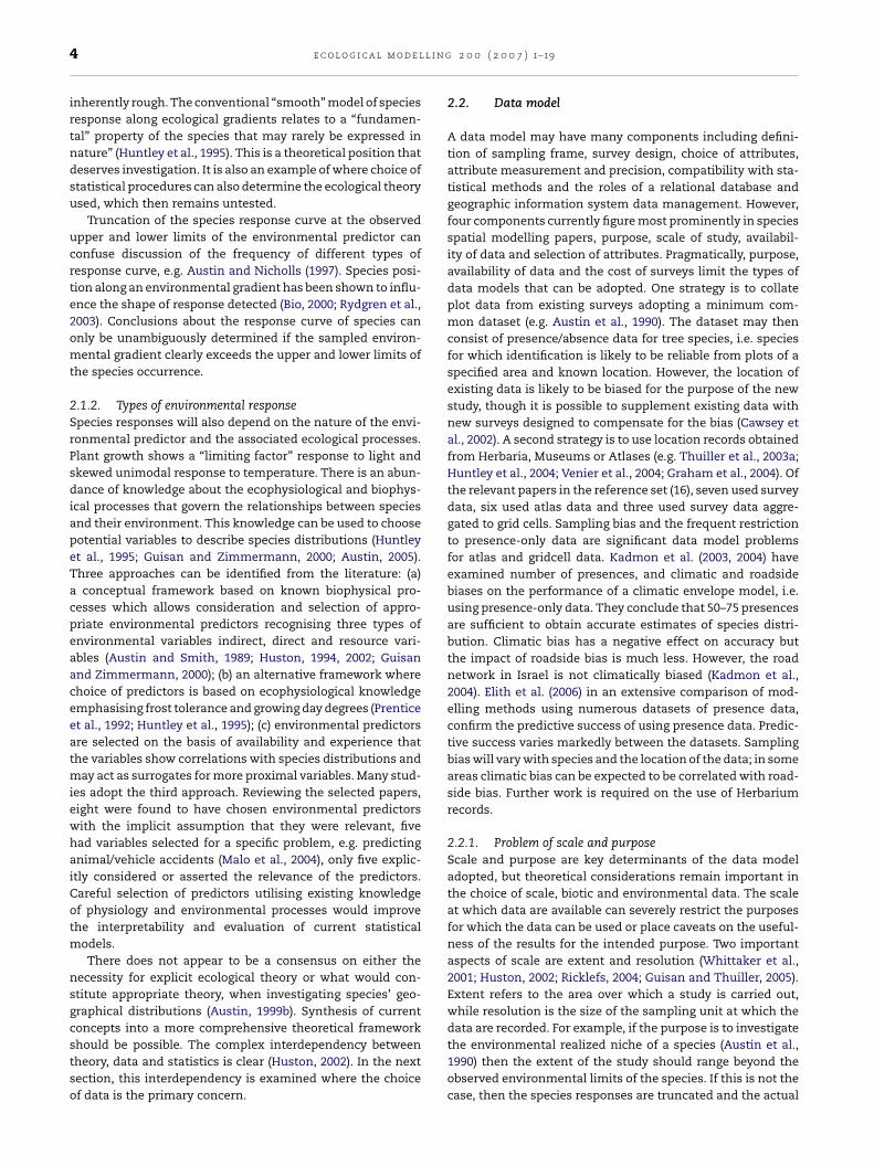

l i n g

4 e c o l o g i c a l m o d e l

inherently rough. The conventional “smooth” model of speciesresponse along ecological gradients relates to a “fundamen-tal” property of the species that may rarely be expressed innature” (Huntley et al., 1995). This is a theoretical position thatdeserves investigation. It is also an example of where choice ofstatistical procedures can also determine the ecological theoryused, which then remains untested.

Truncation of the species response curve at the observedupper and lower limits of the environmental predictor canconfuse discussion of the frequency of different types ofresponse curve, e.g. Austin and Nicholls (1997). Species posi-tion along an environmental gradient has been shown to influ-ence the shape of response detected (Bio, 2000; Rydgren et al.,2003). Conclusions about the response curve of species canonly be unambiguously determined if the sampled environ-mental gradient clearly exceeds the upper and lower limits ofthe species occurrence.

2.1.2. Types of environmental responseSpecies responses will also depend on the nature of the envi-ronmental predictor and the associated ecological processes.Plant growth shows a “limiting factor” response to light andskewed unimodal response to temperature. There is an abun-dance of knowledge about the ecophysiological and biophys-ical processes that govern the relationships between speciesand their environment. This knowledge can be used to choosepotential variables to describe species distributions (Huntleyet al., 1995; Guisan and Zimmermann, 2000; Austin, 2005).Three approaches can be identified from the literature: (a)a conceptual framework based on known biophysical pro-cesses which allows consideration and selection of appro-priate environmental predictors recognising three types ofenvironmental variables indirect, direct and resource vari-ables (Austin and Smith, 1989; Huston, 1994, 2002; Guisanand Zimmermann, 2000); (b) an alternative framework wherechoice of predictors is based on ecophysiological knowledgeemphasising frost tolerance and growing day degrees (Prenticeet al., 1992; Huntley et al., 1995); (c) environmental predictorsare selected on the basis of availability and experience thatthe variables show correlations with species distributions andmay act as surrogates for more proximal variables. Many stud-ies adopt the third approach. Reviewing the selected papers,eight were found to have chosen environmental predictorswith the implicit assumption that they were relevant, fivehad variables selected for a specific problem, e.g. predictinganimal/vehicle accidents (Malo et al., 2004), only five explic-itly considered or asserted the relevance of the predictors.Careful selection of predictors utilising existing knowledgeof physiology and environmental processes would improvethe interpretability and evaluation of current statisticalmodels.

There does not appear to be a consensus on either thenecessity for explicit ecological theory or what would con-stitute appropriate theory, when investigating species’ geo-graphical distributions (Austin, 1999b). Synthesis of currentconcepts into a more comprehensive theoretical framework

should be possible. The complex interdependency betweentheory, data and statistics is clear (Huston, 2002). In the nextsection, this interdependency is examined where the choiceof data is the primary concern.

2 0 0 ( 2 0 0 7 ) 1–19

2.2. Data model

A data model may have many components including defini-tion of sampling frame, survey design, choice of attributes,attribute measurement and precision, compatibility with sta-tistical methods and the roles of a relational database andgeographic information system data management. However,four components currently figure most prominently in speciesspatial modelling papers, purpose, scale of study, availabil-ity of data and selection of attributes. Pragmatically, purpose,availability of data and the cost of surveys limit the types ofdata models that can be adopted. One strategy is to collateplot data from existing surveys adopting a minimum com-mon dataset (e.g. Austin et al., 1990). The dataset may thenconsist of presence/absence data for tree species, i.e. speciesfor which identification is likely to be reliable from plots of aspecified area and known location. However, the location ofexisting data is likely to be biased for the purpose of the newstudy, though it is possible to supplement existing data withnew surveys designed to compensate for the bias (Cawsey etal., 2002). A second strategy is to use location records obtainedfrom Herbaria, Museums or Atlases (e.g. Thuiller et al., 2003a;Huntley et al., 2004; Venier et al., 2004; Graham et al., 2004). Ofthe relevant papers in the reference set (16), seven used surveydata, six used atlas data and three used survey data aggre-gated to grid cells. Sampling bias and the frequent restrictionto presence-only data are significant data model problemsfor atlas and gridcell data. Kadmon et al. (2003, 2004) haveexamined number of presences, and climatic and roadsidebiases on the performance of a climatic envelope model, i.e.using presence-only data. They conclude that 50–75 presencesare sufficient to obtain accurate estimates of species distri-bution. Climatic bias has a negative effect on accuracy butthe impact of roadside bias is much less. However, the roadnetwork in Israel is not climatically biased (Kadmon et al.,2004). Elith et al. (2006) in an extensive comparison of mod-elling methods using numerous datasets of presence data,confirm the predictive success of using presence data. Predic-tive success varies markedly between the datasets. Samplingbias will vary with species and the location of the data; in someareas climatic bias can be expected to be correlated with road-side bias. Further work is required on the use of Herbariumrecords.

2.2.1. Problem of scale and purposeScale and purpose are key determinants of the data modeladopted, but theoretical considerations remain important inthe choice of scale, biotic and environmental data. The scaleat which data are available can severely restrict the purposesfor which the data can be used or place caveats on the useful-ness of the results for the intended purpose. Two importantaspects of scale are extent and resolution (Whittaker et al.,2001; Huston, 2002; Ricklefs, 2004; Guisan and Thuiller, 2005).Extent refers to the area over which a study is carried out,while resolution is the size of the sampling unit at which thedata are recorded. For example, if the purpose is to investigate

the environmental realized niche of a species (Austin et al.,1990) then the extent of the study should range beyond theobserved environmental limits of the species. If this is not thecase, then the species responses are truncated and the actual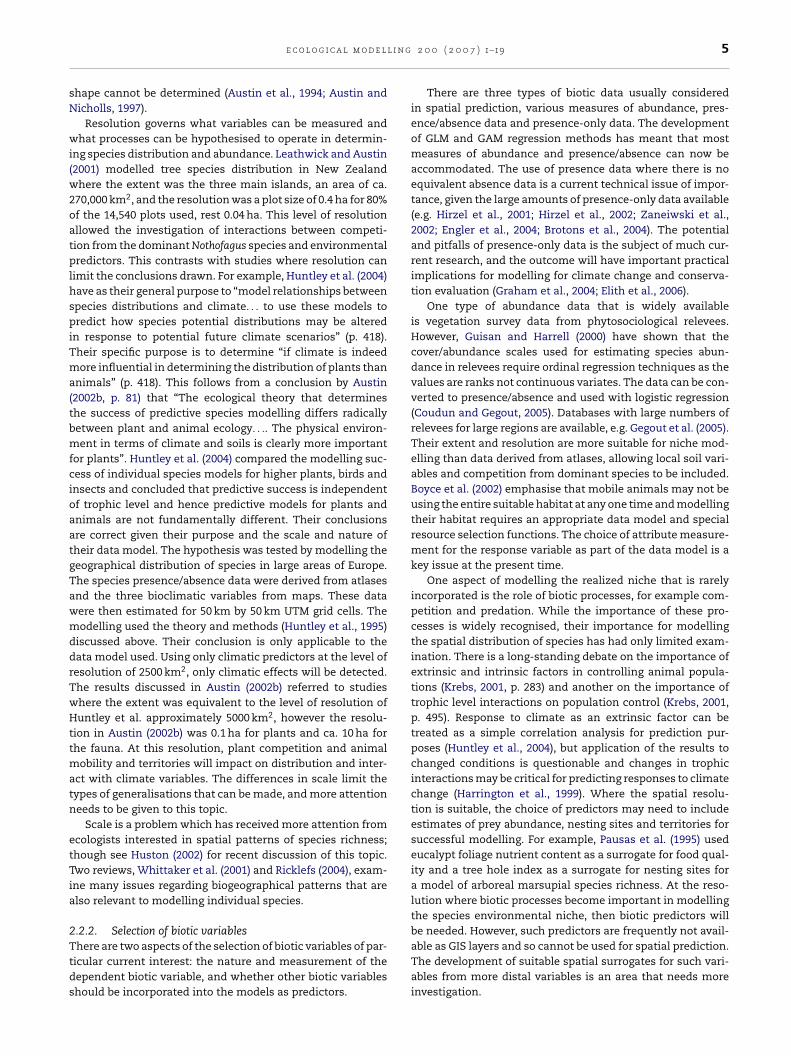

l i n g

sN

wi(w2oatplhspiTma(tbmfcioaatgTawmddrTwHttmatn

etTia

2Ttds

e c o l o g i c a l m o d e l

hape cannot be determined (Austin et al., 1994; Austin andicholls, 1997).

Resolution governs what variables can be measured andhat processes can be hypothesised to operate in determin-

ng species distribution and abundance. Leathwick and Austin2001) modelled tree species distribution in New Zealand

here the extent was the three main islands, an area of ca.70,000 km2, and the resolution was a plot size of 0.4 ha for 80%f the 14,540 plots used, rest 0.04 ha. This level of resolutionllowed the investigation of interactions between competi-ion from the dominant Nothofagus species and environmentalredictors. This contrasts with studies where resolution can

imit the conclusions drawn. For example, Huntley et al. (2004)ave as their general purpose to “model relationships betweenpecies distributions and climate. . . to use these models toredict how species potential distributions may be altered

n response to potential future climate scenarios” (p. 418).heir specific purpose is to determine “if climate is indeedore influential in determining the distribution of plants than

nimals” (p. 418). This follows from a conclusion by Austin2002b, p. 81) that “The ecological theory that determineshe success of predictive species modelling differs radicallyetween plant and animal ecology. . .. The physical environ-ent in terms of climate and soils is clearly more important

or plants”. Huntley et al. (2004) compared the modelling suc-ess of individual species models for higher plants, birds andnsects and concluded that predictive success is independentf trophic level and hence predictive models for plants andnimals are not fundamentally different. Their conclusionsre correct given their purpose and the scale and nature ofheir data model. The hypothesis was tested by modelling theeographical distribution of species in large areas of Europe.he species presence/absence data were derived from atlasesnd the three bioclimatic variables from maps. These dataere then estimated for 50 km by 50 km UTM grid cells. Theodelling used the theory and methods (Huntley et al., 1995)

iscussed above. Their conclusion is only applicable to theata model used. Using only climatic predictors at the level ofesolution of 2500 km2, only climatic effects will be detected.he results discussed in Austin (2002b) referred to studieshere the extent was equivalent to the level of resolution ofuntley et al. approximately 5000 km2, however the resolu-

ion in Austin (2002b) was 0.1 ha for plants and ca. 10 ha forhe fauna. At this resolution, plant competition and animal

obility and territories will impact on distribution and inter-ct with climate variables. The differences in scale limit theypes of generalisations that can be made, and more attentioneeds to be given to this topic.

Scale is a problem which has received more attention fromcologists interested in spatial patterns of species richness;hough see Huston (2002) for recent discussion of this topic.wo reviews, Whittaker et al. (2001) and Ricklefs (2004), exam-ne many issues regarding biogeographical patterns that arelso relevant to modelling individual species.

.2.2. Selection of biotic variables

here are two aspects of the selection of biotic variables of par-

icular current interest: the nature and measurement of theependent biotic variable, and whether other biotic variableshould be incorporated into the models as predictors.

2 0 0 ( 2 0 0 7 ) 1–19 5

There are three types of biotic data usually consideredin spatial prediction, various measures of abundance, pres-ence/absence data and presence-only data. The developmentof GLM and GAM regression methods has meant that mostmeasures of abundance and presence/absence can now beaccommodated. The use of presence data where there is noequivalent absence data is a current technical issue of impor-tance, given the large amounts of presence-only data available(e.g. Hirzel et al., 2001; Hirzel et al., 2002; Zaneiwski et al.,2002; Engler et al., 2004; Brotons et al., 2004). The potentialand pitfalls of presence-only data is the subject of much cur-rent research, and the outcome will have important practicalimplications for modelling for climate change and conserva-tion evaluation (Graham et al., 2004; Elith et al., 2006).

One type of abundance data that is widely availableis vegetation survey data from phytosociological relevees.However, Guisan and Harrell (2000) have shown that thecover/abundance scales used for estimating species abun-dance in relevees require ordinal regression techniques as thevalues are ranks not continuous variates. The data can be con-verted to presence/absence and used with logistic regression(Coudun and Gegout, 2005). Databases with large numbers ofrelevees for large regions are available, e.g. Gegout et al. (2005).Their extent and resolution are more suitable for niche mod-elling than data derived from atlases, allowing local soil vari-ables and competition from dominant species to be included.Boyce et al. (2002) emphasise that mobile animals may not beusing the entire suitable habitat at any one time and modellingtheir habitat requires an appropriate data model and specialresource selection functions. The choice of attribute measure-ment for the response variable as part of the data model is akey issue at the present time.

One aspect of modelling the realized niche that is rarelyincorporated is the role of biotic processes, for example com-petition and predation. While the importance of these pro-cesses is widely recognised, their importance for modellingthe spatial distribution of species has had only limited exam-ination. There is a long-standing debate on the importance ofextrinsic and intrinsic factors in controlling animal popula-tions (Krebs, 2001, p. 283) and another on the importance oftrophic level interactions on population control (Krebs, 2001,p. 495). Response to climate as an extrinsic factor can betreated as a simple correlation analysis for prediction pur-poses (Huntley et al., 2004), but application of the results tochanged conditions is questionable and changes in trophicinteractions may be critical for predicting responses to climatechange (Harrington et al., 1999). Where the spatial resolu-tion is suitable, the choice of predictors may need to includeestimates of prey abundance, nesting sites and territories forsuccessful modelling. For example, Pausas et al. (1995) usedeucalypt foliage nutrient content as a surrogate for food qual-ity and a tree hole index as a surrogate for nesting sites fora model of arboreal marsupial species richness. At the reso-lution where biotic processes become important in modellingthe species environmental niche, then biotic predictors willbe needed. However, such predictors are frequently not avail-

able as GIS layers and so cannot be used for spatial prediction.The development of suitable spatial surrogates for such vari-ables from more distal variables is an area that needs moreinvestigation.

l i n g

6 e c o l o g i c a l m o d e l

The use of biotic predictors for plants has mainly cen-tred on introducing competition from other similar species.Leathwick and Austin (2001) modelled the distribution of treespecies in New Zealand improving the fit of the GAM modelsby including tree density for the dominant tree genus Nothofa-gus as competition terms in models. They also demonstratedthat competitive influence is a function of the environment;interaction terms between Nothofagus density and the princi-pal environmental predictors, mean annual temperature andwater deficit, further improved the models. In this case, suit-able GIS layers were available for predicting species distribu-tion. Austin (2002a) discusses earlier examples of the use ofcompetition predictors based on dominant species in regres-sion models; see also Leathwick (2002). Further examinationof methods for incorporating competition terms into spatialmodelling is needed.

2.2.3. Selection of environmental predictorsHow predictors are selected depends on the ecological and bio-physical processes thought to influence the biota and againthe availability of data and the purpose of the model. Twoapproaches should be considered if we are to move away fromusing all possible predictors and use existing knowledge tobest advantage. These are the nature of the potential predic-tors whether indirect or direct, and whether we have suitableecophysiological knowledge for choosing predictors.

Recognition of indirect, direct and resource vari-ables (Austin and Smith, 1989; Huston, 1994; Guisan andZimmermann, 2000) can have a profound impact on how eachvariable is used in the modelling approach. Indirect variablessuch as altitude and latitude can only have a correlationwith organisms through their correlation with variables suchas temperature and rainfall that can have a physiologicalimpact on organisms. Because the correlation between indi-rect variables and more direct variables is location specificand need not be linear, there is no theoretical expectationregarding the shape of species responses to indirect variables.Temperature and rainfall are direct variables, while resourcevariables are those which are consumed by organisms, e.g.nitrogen for plants or prey for carnivores. There are theoret-ical expectations/hypotheses about the shapes of responseto these types of variables (Austin and Smith, 1989). Plantresponse to soil nutrients is expected to be hyperbolic wherespecies abundance increases to a level beyond which thereis no further increase, a limiting factor response. Evaluationof species niche models should incorporate a test of whetherthe shape of the response to an environmental predictor isconsistent with expected ecological theory.

Rainfall, while having a direct effect on organisms is adistal variable, where the proximal variable might be wateravailability at the root hair for plants. Biophysical processeslink indirect variables to rainfall and from there via waterbalance models to estimates of moisture stress for plants(Austin, 2005). Recognition of the nature of the predictor helpsto define the type of response to be expected. The frequentinclusion of slope and aspect in species modelling studies is

an example of indirect variables where the physical relation-ship with solar radiation is well known and can be calculatedusing trigonometric functions (e.g. Dubayah and Rich, 1995).Austin (2002a) reviews earlier studies where progressive incor-

2 0 0 ( 2 0 0 7 ) 1–19

poration of more direct and proximal predictors using waterbalance models rather than slope and aspect significantlyimproved regression models describing the environmentalniche of eucalypt species. Leathwick in a series of papers hasdemonstrated the value of such derived proximal predictorsfor examining climate change and forest equilibrium at thescale of New Zealand (Leathwick, 1995, 1998; Leathwick et al.,1996; Leathwick and Whitehead, 2001).

Huntley and colleagues (Huntley et al., 1995, 2004) followingPrentice et al. (1992) select their climatic predictors using a dif-ferent physiological model. Three bioclimatic variables wereselected based on well-known roles in imposing constraintson species distributions. The variables were mean tempera-ture of the coldest month, annual sum of degree-days above5 ◦C and Priestley-Taylor’s ˛ (an estimate of the annual ratio ofactual to potential evapotranspiration) (Prentice et al., 1992).These represent direct variables acting as surrogates for coldtolerance, growing conditions and moisture stress. Resourcevariables were not included. The selection of the temperaturevariables has a better physiological rationale than the usualselection of mean annual temperature with a skewed uni-modal response curve (cf. Austin et al., 1994). However, theshape of these temperature responses is unspecified beyondthe possibility of a threshold effect (Huntley et al., 1995). Forexample, is there an optimal number of growing day-degreesfor a species above which there is no further influence? Inaddition, the predictions resulting from using either growingdegree-days or mean annual temperature may be very similarat a regional scale as these variables are often highly corre-lated. Growing degree-days were shown by Pausas et al. (1997)to have a quadratic relationship to mean annual temperaturewith an r2 of 0.989 for 98 meteorological stations in New SouthWales, Australia. A synthesis of the different approaches toselection and use of environmental predictors described abovemay yield more robust and ecologically more rational speciesmodels.

Error in the environmental variables is ignored in con-ventional regression analysis. Such error can have profoundeffects on the outcomes of models. Van Neil et al. (2004) haverecently drawn attention to the influence of error in digital ele-vation models (DEM) on environmental variables. Measuressuch as slope and aspect are usually calculated from a DEMand then incorporated into a geographical information sys-tem (GIS) from which they are retrieved for modelling. Theauthors conclude that a direct variable, solar radiation may beless prone to error than the indirect variables from which itis calculated aspect and slope. The influence of error in theDEM on species models has been further investigated by VanNeil and Austin (in press). Most studies derive their environ-mental predictors from a GIS. The original errors generated inproducing the estimates for the GIS need careful evaluationbefore predictors are used for modelling.

2.3. Statistical model

Ecologists are very dependent on collaboration with statis-

ticians for the introduction of new statistical theory andmethodology into ecology, e.g. the introduction of GAM by Yeeand Mitchell (1991). Improvements continue to be made withrespect to GAM (Wood and Augustin, 2002; Yee and Mackenzie,

l i n g

2ctpseosms

2Corpp2actti2Tctmmidecea

accceouiBannCawute

duttd

e c o l o g i c a l m o d e l

002). The number of different approaches and techniques dis-ussed in Hastie and Tibshirani (1990) make it clear, however,hat the full array of statistical methods has yet to be incor-orated in the ecological modelling of species distributions,ee also Elith et al. (2006). There are three issues regarding thevaluation of the statistical model used for spatial predictionf plant and animal species: (1) how to compare the numeroustatistical methods available (2) how should the success of theodelling be assessed? (3) how should the compatibility of the

tatistical model with the ecological model be evaluated?

.3.1. Comparison and evaluation of methodsomparison of modelling methods is a problem as new meth-ds are continually being introduced. Multivariate adaptiveegression splines (MARS, Friedman, 1991) is one method withotential because of its handling interactions between theredictors (Moisen and Frescino, 2002; Munoz and Felicisimo,004). Leathwick et al. (2005) have recently compared GAMnd MARS methods incorporating a number of novel pro-edures applied to freshwater fish. They conclude that thewo methods give similar results but that MARS has compu-ational advantages. Leathwick et al. (in press) have exam-ned the use of boosted regression trees (BRT, Friedman et al.,000) as a method for modelling demersal species richness.hey conclude that BRT gives superior predictive performanceompared to GAM even when the latter incorporates interac-ion terms. Phillips et al. (2006) have recently introduced a

aximum entropy method (MAXENT). A distinctly differentethod, generalized dissimilarity modelling (GDM) has been

ntroduced by Ferrier et al. (2002). Elith et al. (2006) provides aescription of each of these and other methods, further ref-rences and information on available software. Other recentomparisons of methods include Maggini et al. (2006), Moisent al. (2006), and Drake et al. (2006); all differ in data modelsnd selection of statistical models.

The comparisons of methods undertaken by differentuthors are rarely if ever comparable. For example, two recentomparisons of methods (Araujo et al., 2005; Elith et al., 2006)ompare 4 and 16 methods respectively but only two are inommon. They have different purposes, evaluation of mod-ls using presence/absence data from different time peri-ds for predicting climate change (Araujo et al., 2005) andsing regression methods with presence-only data to max-

mise use of herbarium and museum records of organisms.oth use GLM with the polynomial expansion x, x2, x3, henceny possible comparison is based on the particular procedureot the general method. There is no reason why GLM couldot have used the sequence x, square-root x, see Austin andunningham (1981). Comparisons of GLM with other methodsre confounded with the particular polynomial function usedith GLM in these papers. Similarly, both groups of authorsse GAM with four degrees of freedom for smoothing thoughhis is not the only option, see Wamelink et al. (2005) for anxample of alternatives.

Araujo et al. (2005) emphasise the need to use indepen-ent data for evaluation. They describe three methods of eval-

ation (they use the term validation): resubstitution wherehe same data is used to calibrate the model and measurehe fit; data-splitting where the data is split into two at ran-om, a calibration set and a evaluation set, and independent

2 0 0 ( 2 0 0 7 ) 1–19 7

validation where a totally independent data set from a dif-ferent region is used. Data-splitting is the current preferredmethod but individual observations may still show spatialauto-correlation (Araujo et al., 2005). The third alternative doesnot seem plausible. Separate regions with the same speciescomplement, ranges and combinations of environmental pre-dictors and ecological history simply do not occur. Elith et al.(2006) adopt a useful compromise. They calibrate with one setof data then evaluate the fit with totally separate data col-lected independently from the same region. Given their pur-pose of evaluating the use of presence data, the calibration setis presence-only and the evaluation set is presence/absence,however the results can be expected to apply to other data.

The comparative evaluation of Elith et al. (2006) is the mostcomprehensive to date. Three groups of methods are recog-nised with different levels of predictive success, the newestmethods BRT, GDM and MAXENT are the best, followed byMARS, GLM, GAM, and new version of GARP (OM-GARP), whileother methods, e.g. GARP, LIVES, BIOCLIM and DOMAIN areless satisfactory. The evaluation is based on AUC the areaunder the receiver operating characteristic (ROC) curve andthe point biserial correlation (Elith et al., 2006). Both measurepredictive success using an independent data set.

Current best practice for assessing model success for pres-ence/absence data is AUC (Pearce and Ferrier, 2000; Rushtonet al., 2004; Thuiller, 2003), while a number of different mea-sures are used for quantitative data (Moisen and Frescino,2002; Moisen et al., 2006). However, all the procedures dependon the relationship between observed and predicted values;that is on predictive success not on explanatory value. Is theshape of the predicted response curve for an environmen-tal predictor ecologically rational? While this question can beaddressed for an individual species model, when large num-bers of species are modelled in one publication, presentationof such graphs is not possible, limiting evaluation of the mod-elling results. Elith et al. (2006) in their online appendix doprovide maps of the predicted distributions for several mod-els for a few species. It is apparent that models with the sameor very similar AUC value may predict very different patternsof distribution. Reliance on AUC as a sufficient test of modelsuccess needs to be re-examined (Termansen et al., 2006).

When maps of observed and predicted geographical distri-butions are presented, evaluation of the environmental pre-dictor model is still not possible (Thuiller, 2003; Thuiller et al.,2003a; Huntley et al., 2004). Some provide the degree of thepolynomial fitted for each predictor (Bustamante and Seoane,2004; Thuiller et al., 2003b) but not their values or signs. A fewprovide the model coefficients so that the response shapescould be reconstructed (Venier et al., 2004). Lehmann et al.(2002a) and Elith et al. (2005) provide suggestions on practi-cal options for presenting results graphically for evaluation.Maggini et al. (2006) and Van Neil and Austin (in press) areunusual in presenting both response curves and map predic-tions. Even if predictive success is high, this does not necessar-ily mean that the shape is rational. The fitting of a cubic poly-nomial for predictor may account well for a skewed response

at low values but also predict high probabilities of occurrenceat high predictor values due to the second inflection point inthe curve. This will occur if observations at high predictor lev-els are sparse even if there are no presences in that region.

l i n g

8 e c o l o g i c a l m o d e l

Austin et al. (2006) provide examples. Ultimately, the decisionrests on whether prediction is the sole purpose or whetherecological rationality is needed when using models for esti-mating the impact of climate change and similar purposes.

2.3.2. Using artificial dataThe major difficulty with evaluating statistical methods andtheir compatibility with ecological theory is that the truemodel is unknown. Comparative evaluations on real data areunsatisfactory because two statistical methods may give dif-ferent models but both may be half-right. The objection toartificial data is that current theory regarding species responsecurves is simplistic and unrealistic. A statistical model whichfails to recover the correct structure even from data con-structed on the basis of a simple theory is unlikely to recoveruseful information from real data. Artificial data allows ques-tions such as: are the correct predictor variables selected, arethe correct response shapes found, what are the most appro-priate statistical tests to use and what are the implicationsof using direct or indirect environmental predictors (Austin etal., 2006)?

For example, Bio (2000) generated artificial data sets withthree predictors and species response shapes assuming bell-shaped responses to examine relative performance of themodel selection criteria. She found that the likelihood ratiotest performed better than Akaike’s information criterion (AIC)and the Bayesian information criterion at recovering the truemodel. The use of AIC produced more complicated modelsthan the true model. This generalisation however was sensi-tive to the position of the species on the simulated gradient.Maggini et al. (2006) also examine this issue with similar con-clusions.

Austin et al. (2006) consider the use of artificial data forevaluating statistical models where the true model is knownin detail (Austin et al., 1995 provide greater detail on dataconstruction). They generated sets of artificial data basedon two theories of species response shape, and two sets ofpredictors direct and indirect with explicit biophysical rela-tionships between them. The two theoretical models wereSwan/ter Braak model which assumes equally spaced bell-shaped resonse curves along environmental gradients andthe Ellenberg/Minchin model which allows for a range ofskewed response curves (Austin et al., 2006). The environmen-tal gradients assumed were based on direct variables and theirassociated indirect variables. For example, aspect and slopedetermine the radiation climate of a site: using radiation (adirect variable), or aspect, (an indirect variable) will give riseto very different types of model. Fitting radiation as a predic-tor may result in a unimodal quadratic response function fora species. The equivalent model using aspect in place of radi-ation requires a bimodal response curve for the same species(Austin et al., 2006). Results also indicate that a random vari-able can easily be incorporated into a GLM or GAM model as asignificant predictor. However, inspection of the shape of theresponse and its standard error would lead to recognition ofthe problem. The response is flat and not obviously different

from zero. Skilled analysis of results and residuals is neces-sary to “discover” the “true model” for an individual species.The fitting of large numbers of models for numerous specieswith default settings for the method is not a process which

2 0 0 ( 2 0 0 7 ) 1–19

will find the most appropriate ecological model. Conventionalmodelling with indirect variables was found to be less suc-cessful than with direct variables and could lead to irrationalresponse curves.

The main conclusion from the study described above is thatsuccessful recovery of the true model depends more on theecological insight and statistical skill of the modellers thanthe particular statistical modelling method used (Austin et al.,2006). However, the work raises significant issues of how todesign and evaluate comparative studies of this kind wheresuccess is not simply based on predictive ability.

3. Alternative approaches and models

The review above concerns the current paradigms being usedin the spatial prediction of species distributions and estima-tion of their realised environmental niche. The question needsto be addressed, are there other approaches being used in ecol-ogy and statistics which could improve our research? Are therestatistical methods that have been neglected but are moreconsistent with ecological theory, our knowledge of biophysi-cal processes or the problem of spatial autocorrelation? Threeapproaches requiring more attention are discussed below.

3.1. Liebig’s law of the minimum and quantileregression

Huston (2002), in an introductory essay at the conference on“Predicting Species Occurrences: Issues of accuracy and scale”(Scott et al., 2002), drew attention to the impact of assum-ing Liebig’s Law of the Minimum is operating when modellingspecies response to environmental predictors and then pre-dicting their spatial distribution. Van der Ploeg et al. (1999)provide a modern account of the origins of the Law. One state-ment of the Law would be “plant growth will be limited bythe nutrient in shortest supply even when other nutrients areabundant, giving rise to a hyperbolic response curves to indi-vidual nutrients”. If other resources are less than optimal forsome observations as is usual for field observations as opposedto experiments, observed species performance will be lessthan the maximal possible response to the first resource. Infact, typical regression analyses fitted to the mean values maynot even reflect the true shape of the response to the firstresource.

A number of authors have been addressing this type ofresponse problem in a variety of ecological contexts. Kaiseret al. (1994) drew attention to the “Law of the Minimum”problem with respect to phosphorus limitations to algalbiomass as measured by chlorophyll content in lakes, arguingthat simple least-squares linear regression was inappropri-ate. Thomson et al. (1996) also argued that: “Conventionalcorrelation analysis. . . fundamentally conflicts with the basicconcept of limiting factors” in a study of the spatial distri-bution of Erythronium grandiflorum (Glacier lily) in relation tosoil properties and gopher disturbance. Scharf et al. (1998),

in investigating patterns between prey size and predatorsize in animal populations, considered a related problemestimating the upper and lower boundaries of scatter plotsof the two variables. These three groups of authors all used

l i n g

dtteoamtatao(bs

FhqBfbp

e c o l o g i c a l m o d e l

ifferent analytical approaches, while acknowledging thatheir methods were not entirely satisfactory. Cade et al. (1999)hen presented the use of quantile regression (see also Scharft al., 1998) for the purpose of estimating envelope curvesr “factor-ceiling responses” (Thomson et al., 1996). Cadend Noon (2003) provide a clear exposition of the statisticalethod and its potential for ecological analysis of observa-

ional data for both plants and animals. Figure one providesn artificial example, showing the expected response underhe equivalent of experimental conditions (Fig. 1a) and thens expected in observational field studies (Fig. 1b). Estimates

f the slopes of the responses based on the 10th or 50th

approximates the least-squares regression) quantiles woulde much lower than those from the 90th would. Huston (2002)hows a similar but more complex example. This approach is

ig. 1 – Artificial example of biomass relationship withabitat condition showing 10th, 50th, 75th, 90th and 95thuantiles estimated from quantile regression. (a)iomass/habitat relationship uninfluenced by non-habitat

actors. (b) Biomass/habitat relationship when influencedy non-habitat limiting factors. From Cade et al. (1999) withermission of Ecological Society of America.

2 0 0 ( 2 0 0 7 ) 1–19 9

not simply about the failure to specify an important predictorin the regression model but also that such variables almostinvariably reduce the abundance of the dependent variableand may thus obscure the nature of the relationship.

Cade and Guo (2000) used quantile regression to studyseedling survival of desert annuals. By estimating enveloperesponse curves (95th and 99th quantiles) of final summerseedling density against initial winter density, they wereable to interpret seedling survival as being determinedby seed supply at low initial densities and by competitiveself-thinning at high densities, consistent with a particularmechanistic model. This result could not have been obtainedfrom conventional statistical analysis of the scatter plotsdue to the numerous low survival values resulting fromother unrecorded limiting factors. Krause-Jensen et al. (2000)examined Eelgrass (Zostera marina) abundance and growthalong a water depth gradient using a less satisfactory methodfor estimating “upper boundaries” (Blackburn et al., 1992)than quantile regression. They did, however, fit quadraticfunctions for Eelgrass biomass and cover in relation to theindirect environmental gradient of depth. Knight and Ackerly(2002) investigated variation in the average nuclear DNAcontent of species across a direct environmental gradient,July maximum temperature (Fig. 2). The scatter plot (Fig. 2a)shows a unimodal envelope curve with other limiting factorsreducing DNA content at intermediate temperatures. Thechanging relationship is clearly summarised by the plot of thechanges in sign, value and significance of the quadratic termwhen regressions for various quantiles are calculated (Fig. 2b).While the normal least-squares polynomial was significantwith a negative quadratic coefficient, the strength of theunimodal response was only captured when the small valuesof DNA influenced by the other non-specified limiting factorswere down-weighted in the upper quantile regressions.

Schroder et al. (2005) apparently provide the first exampleof the application of quantile regression to species abun-dance data in relation to environmental gradients. Theycompare quantile regression curves for 95% quantiles withthe mean response curves using the non-linear responsefunctions of Huisman et al. (1993). The response curves forfen plant species in relation to single predictors like annualflooding duration and phosphate show some dramatic differ-ences between the quantile and mean curves. The quantileresponse curves appear more ecologically rational withoutabrupt thresholds and unexpected shapes. The authors donot make a link with Liebig’s Law.

In fact, Liebig’s Law is not the only ecological hypothesisthat has been put forward to explain species physiologicalresponses to nutrients in general (Rubio et al., 2003). Theseauthors contrast Liebig’s Law with the “multiple limitationhypothesis” (MLH Bloom et al., 1985) which says a plant’sadaptive growth will result in all resources limiting plantgrowth simultaneously. The basic assumption of MLH is thatresources are substitutable for each other at least to someextent (Bloom et al., 1985; Rubio et al., 2003). Rubio et al. (2003)tested experimentally whether responses to pairs of min-

eral nutrients were consistent with either hypothesis. Theyfound that it depended which pairs of nutrients were com-pared, some showed a Liebig response, some a MLH responseand some were indeterminate. If Liebig’s law operates for

10 e c o l o g i c a l m o d e l l i n g 2 0 0 ( 2 0 0 7 ) 1–19

Fig. 2 – (a) The relationship between cell nuclear DNA content (2CDNA) of species and average July maximum temperaturewithin the range of the species. (b) The change in value of the coefficient for the quadratic term (solid dark line) in theprogressive quantile regressions calculated for the data in (a). Note the abrupt change above the 75th quantile. The singledashed line is the estimate for the quadratic coefficient for the least squares regression for the total data and the doubledashed lines are the 95% confidence limits. The grey area represents the 95% confidence interval for the quantile regression

of Bl

estimates. From Knight and Ackerly (2002) with permission

any predictor then there is a strong justification for quantileregression. However, the shape of a species response whenexpressed as a mathematical function implies an ecologicaltheory and the opportunity to test one or more associatedhypotheses. The papers of Huston, 2002, Knight and Ackerly(2002) and Schroder et al. (2005) provide a strong case for theuse of quantile regression for modelling species environmen-tal responses. The experimental study of Rubio et al. (2003)contrasting ecophysiological theories demonstrates that thechoice of mathematical function should not depend on defaultoptions in a software package, nor assume a specific theorylike Liebig’s Law applies in all cases.

3.2. Structural equation modelling (SEM)

Structural equation modelling has been advocated and used ina variety of ecological contexts, ecological genetics and evolu-tion (Mitchell, 1992, 1994), ecosystem function and toxicology(Johnson et al., 1991), comparative ecophysiology (Shipley andLechowicz, 2000), trophic interactions (Marquez et al., 2004),plant species recruitment (Garrido et al., 2005) and rare speciesconservation (Iriondo et al., 2003). Vile et al. (2006) have appliedSEM to study changes in species functional traits during old-field succession. Arhonditsis et al., have combined SEM withBayesian analysis to examine the role of abiotic and biotic pro-cesses on phytoplankton dynamics and water clarity in twolakes. McCune and Grace (2002) provide a detailed introduc-tion to its use in ecology. It does not appear to have been usedto model the spatial distribution of individual species.

Shipley (2000) provides a general definition: “SEM modelsrepresent translations of a series of hypothesised cause-effectrelationships between variables into a composite hypothesisconcerning patterns of statistical dependencies”. He presentsthe advantages of SEM as “. . . can test models that includevariables that cannot be directly observed and measured(so-called latent variables) and for which one must relyon observed indicator variables that contain measurement

errors”. Potentially, SEM overcomes many of the problemsof conventional multiple regression. For example, in conven-tional regression, environmental predictors are assumed to bemeasured without error. By explicitly recognising that correla-

ackwell Publishers.

tions between variables may reflect causal pathways and thatsuch variables may have both direct and indirect effects ona dependent variable, SEM can differentiate between alterna-tive regression models. In fact, an SEM model of a complexset of pathways describing how environmental variables (e.g.Fig. 3) may affect each other and the dependent variable can betested for consistency with the observed data. A hypothesisedset of causal pathways can be rejected if it is not consistentwith the observations.

Shipley (2000) lists the disadvantages of SEM as functionalrelationships must be linear, non-multivariate normal dataare difficult to treat, and large sample sizes are needed. SEMwould provide a means of incorporating knowledge about indi-rect, direct and resource variables (Austin and Smith, 1989)into a hypothesis about the causal pathways linking envi-ronmental variables, biotic influences, e.g. competition andherbivory with the distribution of species. The possibility ofestimating explicitly latent variables also has considerablepotential. Latent variables could be estimates of variablesmore proximal in the causal path than those we can measure(Austin, 2005) and use in multiple regressions.

However, if we equate species richness per plot to theabundance of a species, considering it to be controlled by thesame biotic and abiotic variables then a significant examplehas been published, Grace and Pugesek (1997), which isfurther explained in McCune and Grace (2002). These authorsexamine plant species richness as a function of plant biomass,disturbance and abiotic variables in a coastal wetland. Theyrecognised that abiotic variables such as soil salinity mighthave a direct effect on species richness and an indirect effectvia an effect on plant biomass per plot, which then affectsspecies richness, possibly by reducing light beneath thecanopy. They established an initial SEM model based on suchhypotheses (Fig. 3a), partitioning the correlations betweenthe variables to simultaneously fit the entire data set, not justthe dependent variable species richness. The terminologyused is complex. The following description is based on Grace

and Pugesek (1997). Measured variables (e.g. soil carbon)are referred to as indicators of the latent variables (e.g. soilinfertility). The relationships between the indicator variablesand latent variables constitute the measurement model,

e c o l o g i c a l m o d e l l i n g 2 0 0 ( 2 0 0 7 ) 1–19 11

Fig. 3 – Structural equation model (SEM) for species richness in a coastal wetland. (a) Initial conceptual model. Latentvariables are enclosed in ellipses and indicated (estimated) by measured or indicator variables shown in boxes. Arrowsrepresent possible path coefficients. See Grace and Pugesek (1997) for further details. (b) Final specific model. The pathcoefficients represent standardised partial regression coefficients. Arrows between latent variables and indicators representthe degree to which indicators are correlated with latent variables. Pathways between latent variables show the direction,sign and partial regression coefficients. The pluses and minuses behind the path coefficient for the light-to-richness pathserve as a reminder that this path has strong positive and negative components since it is the transformation of ahump-shaped relationship. The endogenous variables biomass, light and richness are shown to have 70%, 65% and 45% oftheir variance explained by the model. (Figs. 3 and 6 from Grace and Pugesek (1997) from American Naturalist withp

wkv(

ermission).

hile the relationships between the latent variables arenown as the structural model. There are two kinds of latentariable, exogenous those which only predict other variablese.g. flooding) and endogenous those which are dependent on

other variables (e.g. species richness). For further details ofthe statistical procedures used, see McCune and Grace (2002).The results of SEM based on Fig. 3a are shown in Fig. 3b. Notethat while flooding is estimated to have an indirect effect

l i n g 2 0 0 ( 2 0 0 7 ) 1–19

Fig. 4 – Relationship between normalised differencevegetation index (NDVI) and rainfall for 1987 from NorthAfrica and Middle East showing a straight-line ordinaryleast squares regression. Note curvilinear scatter of data

12 e c o l o g i c a l m o d e l

through correlation with biomass there is no evidence thatsalinity does. Disturbance has an effect only through biomassand light at ground level. Species richness is seen as a directand indirect function of environmental variables, the bioticvariable biomass and its dependent variable light, plus anindirect function of disturbance. If abundance of an individualspecies were substituted for species richness in Fig. 3b, theSEM model would appear an entirely feasible approach tomodelling individual species distribution. It would have theadded advantage of making explicit the relationships betweenindirect, direct and resource variables.

The recent papers on the determinants of species rich-ness in different plant communities (Grace and Pugesek, 1997;Weiher, 2003; Weiher et al., 2004) provide interesting resultson the relative importance of environmental variables andbiomass in influencing species richness in different commu-nities. However, these authors use bivariate curvilinear regres-sion to provide functions to linearise the relationship betweenthe principal predictors and species richness as the depen-dent variable prior to analysis. This assumes that no otherpredictor is masking the shape of the relationship. There isan urgent need to evaluate the impact of non-linear rela-tionships (sensu lato) and effects arising from concepts likethe Law of the Minimum on SEM, before it is widely used inmodelling species distribution. Tests with artificial data basedon current ecological theory would provide a suitable initialapproach.

3.3. Spatial non-stationarity and geographicallyweighted regression (GWR)

Spatial autocorrelation, where the abundance or occurrenceof species is correlated with presence and abundance of thespecies nearby, can affect statistical modelling (Cressie, 1993).Specific account of this has been incorporated into speciesmodelling (Smith, 1994; Leathwick, 1998). More recently, theproblem of whether the statistical model remains constantover the spatial extent of a study has been raised (Osborne andSuarez-Seoane, 2002). A statistical procedure, GWR has beendeveloped to examine specifically this issue (Fotheringhamet al., 2002). Biologically, this approach could be of impor-tance as it is a local technique that allows the regressionmodel parameters to vary in space. If species are not in equi-librium with their environment, or if the social behaviourof animals changes with location, then statistical modelsbased on local regions may provide more information and bet-ter predictions than a global model based on data from thewhole study area (Osborne and Suarez-Seoane, 2002; Foody,2004).

A simple ecological example is provided by Foody (2003)where the normalised difference vegetation index (NDVI), aremotely sensed measure of vegetation productivity, is relatedto rainfall for North Africa and the Middle East (Fig. 4). Anexample of avian species richness prediction from three envi-ronmental variables (maximum NDVI, mean annual tempera-ture, total annual precipitation) for sub-Saharan Africa shows

marked spatial variation in regression coefficients (2004).There are clearly major changes in the local regressions andthese vary progressively across southern Africa. There is con-troversy over the relative importance of GWR versus global

points. (Fig. 2a from Foody (2003) Remote Sensing ofEnvironment with permission).

spatial regression compare Jetz and Rahbek (2002) and Foody(2004) for the same species data and see also Jetz et al. (2005)and Foody (2005a) This regression method has yet to be usedfor modelling individual species and needs to be reviewedcarefully before being used.

I use the NDVI example (Foody, 2003) to consider some ofthe problems. Figure four shows the straight-line relationshipfitted to the global data set. However, one would expect thatabove a certain rainfall NDVI would be unresponsive to rain-fall, an application of Liebig’s Law of the Minimum. An equallyparsimonious conventional least-squares regression would beto fit a reciprocal function (1/x). This would approximate anecologically rational response and fit the data better (Fig. 5a).However, as Huston (2002) has pointed out if a limiting factorresponse is theoretically appropriate then quantile regressionmodel is the statistical model to use (Fig. 5b).

If the expected relationship is curvilinear, the applicationof GWR poses a problem. Both NDVI and rainfall show spatialautocorrelation. Fitting a suitable conventional regressionmodel to the variables may well result in residuals withno remaining spatial autocorrelation, all other things beingequal. However, when a local regression is fitted with obser-vations weighted by distance from the location, bias canresult because of the spatial autocorrelation in the predictor.In a high rainfall location, highly weighted observations closeto the location will also have high rainfall and conversely inlow rainfall locations neighbouring observations will havelow rainfall. The consequences in the curvilinear responsemodel could well be as shown in Fig. 5c. In low rainfallregions, a steep linear regression while in high rainfall areas,a flat, non-significant regression, due not to non-stationarityin the relationship but to a curvilinear relationship andspatial autocorrelation in the predictor. Foody (2004, 2005b)investigating bird species richness in Sub-Saharan Africa and

Britain, respectively, using NDVI and temperature fits onlystraight-line functions. Unimodal responses are characteristicof species responses to climatic predictors. In such circum-stances, GWR will effectively subsample limited ranges of

e c o l o g i c a l m o d e l l i n g 2 0 0 ( 2 0 0 7 ) 1–19 13

Fig. 5 – Alternative approaches to analysis of normalised difference vegetation index (NDVI) and rainfall for 1987 from NorthAfrica and Middle East. (a) Parsimonious curvilinear regression (y = a + b/x). (b) Possible 95% quantile parsimoniouscurvilinear regression (y = a + b/x). (c) Potential linear geographical weighted regressions (GWR) from (A): low rainfall region,a weir f rai

ti

e

(

(

(

4

Fne

nd (B): high rainfall region. (d) Potential linear geographicalelationship with rainfall from regions with different levels o

he species distribution producing apparent non-stationaryn the underlying process (Fig. 5d).

The NDVI/rainfall example captures a number of issues rel-vant to spatial modelling of species:

1) the use of straight-line regression that is linear in the vari-ables is inappropriate, when the data and theory suggesta curvilinear response;

2) further consideration of the limiting factor theory clearlyrelevant to NDVI suggests that quantile regression wouldbe the preferred statistical model;

3) methods of spatial autocorrelation and non-stationarity ofprocesses after allowing for curved responses require fur-ther investigation, not least because of their importancefor testing the assumption that species distributions arein equilibrium with current environments.

. Conclusion: best practice?

rom the papers cited in this review, it is clear that there iso standard for current best practice when modelling speciesnvironmental niche or geographical distribution, whether

ghted regressions (GWR) for a species showing a unimodalnfall (a–c) modified from Foody (2003) see Fig. 4.

plant or animal. Numerous incompatibilities between the eco-logical, data and statistical models can be identified. Newideas on how to proceed, such as Huston’s (2002) suggestionof using Liebig’s Law of the Minimum and quantile regression,Grace and Pugesek’s (1997) ideas on the use of SEM and therole of GWR (Foody, 2004) to investigate spatial dependency,all require further development and investigation before theycan be used on a routine basis. Can any recommendations bemade?

There are now numerous reports that skewed responsecurves are frequent (Bio et al., 1998; Ejrnaes, 2000; Rydgren etal., 2003), supporting expectations from ecological theory. Bestpractice would therefore be to test for such responses using aGAM model or similar procedure and not assume straight lineor quadratic functions without explicit theoretical justifica-tion. GRASP (Lehmann et al., 2002b) is one software packagethat provides a series of tools for exploring possible responsesbefore modelling. Recent applications of new statistical proce-dures for modelling (Moisen et al., 2006; Munoz and Felicisimo,2004; Elith et al., 2006) expand the potential for examining

the complex curves and interactions that may be postulatedby ecological theory (Austin and Smith, 1989) or detected byexploratory modelling. Understanding the interrelationshipbetween ecological theory, statistical theory and the relative

l i n g

14 e c o l o g i c a l m o d e l

performance of statistical models is a complex issue. Artifi-cial data offers one means of examining these issues mak-ing explicit both ecological and statistical assumptions (Bio,2000; Austin et al., 2006). Their results indicate that all statis-tical procedures should be tested with realistic artificial databefore being adopted as current practice. However, Austin etal. (2006) also conclude that ecological insight and statisticalskill are more important than the precise methodology usedwhen searching for the true model in artificial data.

Defining best current practice for modelling species distri-butions faces great problems (Huston, 2002; Cade et al., 2005).Ecological theory suggests that environmental predictorsmust be evaluated in terms of Liebig’s Law of the Minimum,the multiple limitation hypothesis and the expected shapeof response. The Law will apply to some resource variables;others may be substituteable (Rubio et al., 2003) However,nutrient resources can also occur in toxic excess. Responseto the direct but distal variable, temperature may reflect frostdamage at low temperature while high temperature damagereflects protein denaturation. Exactly how predictors are likelyto influence species will depend on whether they are indirect,direct or resource variables, proximal or distal, abiotic or biotic(Austin and Smith, 1989; Grace and Pugesek, 1997). Regressionmodelling rarely if ever examines correlation of variables interms of process. Recognition of the type of variable can havea dramatic effect on the type of response curve which might beexpected (Austin et al., 2006). Setting up a SEM with a detailedhypothetical path analysis (Fig. 3) when selecting predictorswould make explicit the nature of the predictors and theirlikely inter-dependence. The possibility of using known bio-physical process knowledge to estimate more proximal latentvariables could be assessed against depending on indirect sur-rogate variables such as slope.

The different ecophysiological assumptions currentlyinfluencing selection of environmental predictors (Austin andSmith, 1989; Huntley et al., 1995; Leathwick and Whitehead,2001; Huston, 2002) need to be justified in more detail, e.g.Bloom et al. (1985) and Rubio et al. (2003). The expectation isthat predictors representing light, nutrients, water and tem-perature will influence plant distribution. Excluding predictorsfor one of these factors needs to be justified. Ecological judge-ment will have to be exercised over what to include and whatneeds to be justified.

One example of exercising ecological judgement whenintegrating ecological theory with statistical models is intro-ducing competition between plant species. Logically, the mostappropriate statistical model would be simultaneous regres-sion where interaction (competition or facilitation) coeffi-cients between all species are estimated along with the envi-ronmental predictors (Brzeziecki, 1987). However, the plot sizeof vegetation data is usually large relative to the size of indi-vidual plants and in most cases, rare species will not occuradjacent to each other and hence are unable to compete. Insuch circumstances, competition coefficients are inappropri-ate and cannot be calculated. As species abundance increasesrelative to plot size, the probability of species occurring as

neighbours will increase and species interactions becomemore likely. Identification of the possible occurrence of com-petition using regression models will be a function of plantsizes, abundances and spatial pattern relative to plot size.

2 0 0 ( 2 0 0 7 ) 1–19

This reasoning provides an explanation of the success of thoseregression models of a species discussed by Austin (2002a)where the model fit increased dramatically when the veg-etation was stratified by plant community and the abun-dance of the dominant species of each community intro-duced as an additional predictor of the realised niche of thespecies. Leathwick (2002) has demonstrated both competitiveand facilitative interactions between the dominant Nothofagusspecies conditional on environment in New Zealand forests.However, introducing such an ecological process as competi-tion will depend critically on the data model adopted. Choiceof plot size relative to the scale of the process and availabil-ity of abundance data will determine the feasibility of suchmodelling.

Examples of using ecological and physiological knowledgeto design the ecological, data and statistical models couldbe multiplied. The outcome of applying these ideas will bemodels that are more robust, include ecologically more ratio-nal responses and better prediction. Similar progress is beingmade with the data model and statistical model, but agreedstandards for best current practice appear unlikely in the nearfuture based on the review of literature presented here.

The three potential areas where progress might be madehave been suggested, quantile regression, SEM and GWR.Quantile regression appears to have a sound basis in eco-logical and statistical theory, and software is available (Cadeand Noon, 2003). A version is also available for nonparametric,nonlinear smoothers (Yu and Jones, 1998 quoted in Cade andNoon, 2003, see also Schroder et al., 2005). The only applica-tion to species modelling of quantile regression by Schroderet al. (2005) uses only a single predictor variable at a time dueto the limited amount of data. A case study of its applicationto modelling of species spatial distribution using numerousenvironmental predictors is needed.

Structural equation modelling has an appealing concep-tual framework with the possibility of testing whether data isconsistent with a hypothesised causal pathway (Shipley, 1999).The limitation of SEM to linear relationships, multivariate nor-mal data and preferably large data sets (Shipley, 2000) seems torestrict its potential for spatial prediction. Grace and Pugesek(1997) and Vile et al. (2006) apply data transformations to lin-earise individual relationships between variables. Arhonditsiset al. (2006) claim that non-linear relationships can be accom-modated. It is beyond the competence of the present reviewerto review the statistical aspects of SEM, but it does appearto have problems dealing with curvilinear relationships andinteractions (Schumacker and Marcoulides, 1998; Lee et al.,2004). The previous discussion on GWR (Fig. 5) makes it clearthat the method cannot distinguish between non-stationarityof process and curvilinear relationships between predictorand dependent variables. This does not mean it cannot beused for exploratory data analysis; regions of rapid changeof parameters still need to be investigated and understood.Spatial autocorrelation remains an important issue for spatialprediction of species distribution.

Improved communications between the existing research

paradigms is needed. Certain “rules of thumb” can be applied:

1. Investigate the possibility of curvilinear relationships(sensu lato).

i n g

2

3

4

5

6

7

8

9

mcpm

satipidserMldgtaL2si

aptaetaiTw2hraet

r

environmental gradients. Proc. Ecol. Soc. Austr. 11, 109–119.Austin, M.P., Nicholls, A.O., 1997. To fix or not to fix the species

limits, that is the ecological question: response to Jari

e c o l o g i c a l m o d e l l

. State explicitly what ecological theory is being assumed ortested.

. Ensure that data resolution is consistent with theory andthe predictors being used.

. Examine relationships between variables for environmen-tal process interactions in order to derive more proximalpredictors.

. Evaluate new methods with realistic artificial data, i.e. dataconsistent with current ecological understanding.

. Use more than one statistical method to build the predic-tive model.

. Do not depend solely on prediction success when evaluat-ing species models.

. Investigate the model residuals for spatial and other pat-terns.

. Use independent data to test the models.

Many of these “rules” should be used routinely. Othersight use terminology that is more sophisticated when dis-

ussing analytical technique but what is important is the com-atibility between the ecological questions and the statisticalethodology.These regression models test whether there is a relation-

hip between certain hypothesised environmental predictorsnd species occurrence. The models provide a predictive equa-ion with which the data are consistent. The models do notmply causation. There is a reasonable presumption that theredictors are surrogates for causal processes based on ecolog-

cal knowledge. However, disproving such presumptions posesifficulties. Few manipulative experimental tests of regres-ion models have been attempted. McCune et al. (2003) mod-lled lichen distributions in relation to elevation using logisticegression and a kernel smoother. Subsequently, Antoine andcCune (2004) modelled the vertical height distribution of

ichens within the forest canopy. They then compared theseistribution curves with those obtained from the biomassrowth of lichens derived from transplant experiments withinhe forest canopy. Two species showed consistent responses,bundance and growth followed similar curves. One speciesobaria oregana was inconsistent. Maximum abundance was at5–30 m but maximum growth was at 40–45 m. Two hypothe-es were advanced, competition or establishment. Such exper-mental tests will only be possible with certain organisms.

Process models are often advocated as an alternativepproach to statistical models. Deductive testing of possiblerocesses without adequate description of the pattern is likelyo be inefficient. Statistical models of species occurrence offer

solution. They provide a statement of the potentially rel-vant environmental variables that need to be included inhe process models and their relative importance. An iter-tive procedure between the process and statistical modelss needed with each model acting as a test of the other.his approach is implicit in the recent studies of Leath-ick (Leathwick and Whitehead, 2001; Leathwick and Austin,

001; Leathwick, 2002) but needs to be made explicit. Theypothesised causal path model or SEM shown in Fig. 3 rep-

esents such an explicit statement. Both Grace (in McCunend Grace, 2002) and Shipley (1999, 2000) have also arguedxplicitly for this approach. Yet, the potential of SEM foresting models of species distribution will remain uncertain

2 0 0 ( 2 0 0 7 ) 1–19 15

until it is demonstrated that the approach can deal with thenumerous curvilinear responses that are commonly foundin species/environment relationships (cf. Lee et al., 2004).Species distribution models are important in applied ecologybut progress in the development and use will require constantevaluation.

This review is critical of our current progress in achievingan appropriate synthesis of our ecological theory, data mod-els and statistical methods. However, there are many goodideas, methods and appropriate data sets in the differentresearch paradigms operating in the area of species modellingwhich could contribute to a synthesis. Such a synthesis wouldimprove our predictions and hence management of our natu-ral resources.

Acknowledgements

I thank P. Gibbons, A.O. Nicholls, C.J. Krebs and K. Van Neilfor comments on the manuscript and the CSIRO SustainableSystems librarians for their help with references. This paperformed part of the Riederalp 2004 Workshop on GeneralizedRegression and Spatial Prediction and I thank the organisersA. Guisan, A. Lehmann, J. Overton, S. Ferrier and R. Aspinallfor the invitation to attend.

e f e r e n c e s*

Antoine, M.E., McCune, B., 2004. Contrasting fundamental andrealized ecological niches with epiphytic lichen transplants inan old-growth Pseudotsuga forest. Bryologist 107, 163–173.

Araujo, M.B., Pearson, R.G., Thuiller, W., Erhard, M., 2005.Validation of species-climate impact models under climatechange. Global Change Biol. 11, 1504–1513.

Arhonditsis, G.B., Stow, C.A., Steinberg, L.J., Kenney, M.A.,Lathrop, R.C., McBride, S.J., Reckhow, K.H., 2006. Exploringecological patterns with structural equation modelling andBayesian analysis. Ecol. Model. 192, 385–409.

Austin, M.P., 1999a. A silent clash of paradigms: someinconsistencies in community ecology. Oikos 86, 170–178.

Austin, M.P., 1999b. The potential contribution of vegetationecology to biodiversity research. Ecography 22, 465–484.

Austin, M.P., 2002a. Spatial prediction of species distribution: aninterface between ecological theory and statistical modelling.Ecol. Model. 157, 101–118.

Austin, M.P., 2002b. Case studies of the use of environmentalgradients in vegetation and fauna modelling: theory andpractice in Australia and New Zealand. In: Scott, J.M.,Heglund, P.J., Samson, F., Haufler, J., Morrison, M., Raphael, M.,Wall, B. (Eds.), Predicting Species Occurrences: Issues ofAccuracy and Scale. Island Press, Covelo, California, pp. 73–82.

Austin, M.P., 2005. Vegetation and environment: discontinuitiesand continuities. In: van der Maarel, E. (Ed.), VegetationEcology. Blackwell Publishing, Oxford, pp. 52–84.

Austin, M.P., Cunningham, R.B., 1981. Observational analysis of

Oksanen. J. Veg. Sci. 8, 743–748.

∗ References used in review in section on current models for pre-dicting species distributions.

l i n

16 e c o l o g i c a l m o d e l

Austin, M.P., Smith, T.M., 1989. A new model for the continuumconcept. Vegetatio 83, 35–47.

Austin, M.P., Nicholls, A.O., Margules, C.R., 1990. Measurement ofthe realised qualitative niche: environmental niches of fiveEucalyptus species. Ecol. Monogr. 60, 161–177.

Austin, M.P., Belbin, L. Meyers, J.A., Doherty, M.D., Luoto, M.(2006). Evaluation of statistical models for predicting plantspecies distributions: role of artificial data and theory. Ecol.Model., doi:10.1016/j.ecolmodel.2006.05.023, in press.

Austin, M.P., Nicholls, A.O., Doherty, M.D., Meyers, J.A., 1994.Determining species response functions to an environmentalgradient by means of a �-function. J. Veg. Sci. 5, 215–228.

Austin, M.P., Meyers, J.A., Belbin, L., Doherty, M.D., 1995. Modellingof landscape patterns and processes using biological data.Subproject 5: simulated data case study. Consultancy Reportfor ERIN, CSIRO Wildlife and Ecology, Canberra.

*Bhattarai, K.R., Vetaas, O.R., Grytnes, J.A., 2004. Fern speciesrichness along a central Himalayan elevational gradient,Nepal. J. Biogeogr. 31, 389–400.

Bio, A.M.F., 2000. Does vegetation suit our models? Data andmodel assumptions and the assessment of speciesdistribution in space. Faculteit Ruimtelijke WetenschappenUniversiteit Utrecht. Nederlandse Geografische Studies 265.

Bio, A., Alkemade, R., Barendregt, A., 1998. Determiningalternative models for vegetation response analysis: anon-parametric approach. J. Veg. Sci. 9, 5–16.

Blackburn, T.M., Lawton, J.H., Perry, J.N., 1992. A method ofestimating the slope of upper bounds of plots of body size andabundance in natural animal assemblages. Oikos 65, 107–112.

Bloom, A.J., Chapin, F.S., Mooney, H.A., 1985. Resourcelimitationin plants-an economic analogy. Ann. Rev. Ecol. Syst.16, 363–392.

Boyce, M.S., Vernier, P.R., Nielson, S.E., Schmiegelow, F.K.A., 2002.Evaluating resource selection functions. Ecol. Model. 157,281–300.

Brotons, L., Thuiller, W., Araujo, M.B., Hirzel, A.H., 2004.Presence-absence versus presence-only modelling methodsfor predicting bird habitat suitability. Ecography 27, 437–448.

*Bustamante, J., Seoane, J., 2004. Predicting the distribution offour species of raptors (Aves: Accipitridae) in southern Spain:statistical models work better than existing maps. J. Biogeogr.31, 295–306.

Brzeziecki, B., 1987. Analysis of vegetation–environmentrelationships using a simultaneous equations model.Vegetatio 71, 175–184.

Cade, B.S., Guo, Q., 2000. Estimating effects of constraints on plantperformance with regression quantiles. Oikos 91, 245–254.

Cade, B.S., Noon, B.R., 2003. A gentle introduction to quantileregression for ecologists. Front. Ecol. Environ. 1, 412–420.

Cade, B.S., Noon, B.R., Flather, C.H., 2005. Quantile regressionreveals hidden bias and uncertainty in habitat models.Ecology 86, 786–800.

Cade, B.S., Terrell, J.W., Schroeder, R.L., 1999. Estimating effects oflimiting factors with regression quantiles. Ecology 80, 311–323.

Cawsey, E.M., Austin, M.P., Baker, B.L., 2002. Regional vegetationmapping in Australia: a case study in the practical use ofstatistical modelling. Biodivers. Conserv. 11, 2239–2274.

*Clarke, E.D., Spear, L.B., McCracken, M.L., Marques, F.F.C.,Brochers, D.L., Buckland, S.T., Ainley, D.G., 2003. Validating theuse of generalized additive models and at-sea surveys toestimate size and temporal trends of seabird populations. J.Appl. Ecol. 40, 278–292.

Cleveland, W.S., Devlin, S.J., 1988. Locally weighted regression: anapproach to regression analysis by local fitting. J. Am. Stat.Assoc. 83, 596–610.

Coudun, C., Gegout, J., 2005. Ecological behaviour of herbaceousforest species along a pH gradient: a comparison betweenoceanic and semicontinental regions in northern France.Global Ecol. Biogeogr. 14, 263–270.

g 2 0 0 ( 2 0 0 7 ) 1–19

Cressie, N.A.C., 1993. Statistics for Spatial Data. Wiley, New York.Drake, J.M., Randin, C., Guisan, A., 2006. Modelling ecological

niches with support vector machines. J. Appl. Ecol. 43,424–432.

Dubayah, R., Rich, P.M., 1995. Topographic solar radiation modelsfor GIS. Int. J. Geogr. Inf. Syst. 9, 405–419.

Elith, E., Burgman, M.A., Regan, H.M., 2002. Mapping epistemicuncertainties and vague concepts in predictions of speciesdistribution. Ecol. Model. 157, 313–329.

Elith, J., Ferrier, S., Huettmann, F., Leathwick, J., 2005. Theevaluation strip: a new and robust method for plottingpredicted responses from species distribution models. Ecol.Model. 186, 280–289.

Elith, J., et al., 2006. Novel methods improve prediction of speciesdistributions from occurrence data. Ecography 29, 129–151.

*Engler, R., Guisan, A., Rechsteiner, L., 2004. An improvedapproach for predicting the distribution of rare andendangered species from occurrence and pseudo-absencedata. J. Appl. Ecol. 41, 263–274.

Ejrnaes, R., 2000. Can we trust gradients extracted by detrendedcorrespondence analysis? J. Veg. Sci. 11,565–572.

Ferrier, S., Watson, G., Pearce, J., Drielsma, M., 2002. Extendedstatistical approaches to modelling spatial pattern inbiodiversity in northeast New South Wales. 1. Species-levelmodelling. Biodivers. Conserv. 11, 2275–2307.

Fitzgerald, R.W., Lees, B.G., 1992. The application of neuralnetworks to the floristic classification of remote sensing andGIS data in complex terrain. In: Proceedings of the XVIICongress of the International Society for Photogrammetryand Remote Sensing, Washington, USA, pp. 570–573.

Foody, G.M., 2003. Geographical weighting as a further refinementto regression modelling: An example focused on theNDVI-rainfall relationship. Remote Sens. Environ. 88, 283–293.

Foody, G.M., 2004. Spatial nonstationarity and scale-dependencyin the relationship between species richness andenvironmental determinants for the sub-Saharan endemicavifauna. Global Ecol. Biogeogr. 13, 315–320.

Foody, G.M., 2005a. Clarifications on local and global dataanalysis. Global Ecol. Biogeogr. 14, 99–100.

Foody, G.M., 2005b. Mapping the richness and composition ofBritish breeding birds from coarse spatial resolution satellitesensor imagery. Int. J. Remote Sens. 26, 3943–3956.

Fotheringham, A.S., Brunsdon, C., Charlton, M., 2002.Geographical Weighted Regression: The Analysis of SpatiallyRelationships. Wiley, Chichester.

Franklin, J., 1995. Predictive vegetation mapping: geographicmodelling of biospatial patterns in relation to environmentalgradients. Prog. Phys. Geogr. 19, 474–499.

Friedman, J.H., 1991. Multivariate adaptive regression splines.Ann. Stat. 19, 1–141 (with discussion).

Friedman, J.H., Hastie, T., Tibshirani, R., 2000. Additve logisticregression: a statistical view of boosting. Ann. Stat. 28,337–407.

Garrido, J.L., Rey, P.J., Herrera, C.M., 2005. Pre- andpost-germination determinants of spatial variation inrecruitment in the perennial herb Helleborus foetidus L.(Ranunculaceae). J. Ecol. 93, 60–66.

Gegout, J., Coudon, C., Bailly, G., Jabiol, B., 2005. EcoPlant: A forestsite database linking floristic data with soil and climatevariables. J. Veg. Sci. 16, 257–260.

*Gibson, L.A., Wilson, B.A., Cahill, D.M., Hill, J., 2004. Spatialprediction of rufous bristlebird habitat in a coastal heathland:a GIS-based approach. J. Appl. Ecol. 41, 213–223.

Giller, J., 1984. Community Structure and the Niche. Chapman

and Hall, London.

Grace, J.B., Pugesek, B.H., 1997. A structural equation model ofplant species richness and its application to a coastalwetland. Am. Nat. 149, 436–460.

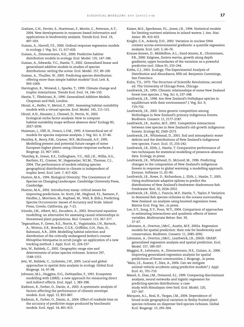
i n g

e c o l o g i c a l m o d e l l

Graham, C.H., Ferrier, S., Huettman, F., Moritz, C., Peterson, A.T.,2004. New developments in museum-based informatics andapplications in biodiversity analysis. Trends Ecol. Evol. 19,497–503.

Guisan, A., Harrell, F.E., 2000. Ordinal response regression modelsin ecology. J. Veg. Sci. 11, 617–626.

Guisan, A., Zimmermann, N.E., 2000. Predictive habitatdistribution models in ecology. Ecol. Model. 135, 147–186.

Guisan, A., Edwards, T.C., Hastie, T., 2002. Generalized linear andgeneralized additive models in studies of speciesdistributions: setting the scene. Ecol. Model. 157, 89–100.

Guisan, A., Thuiller, W., 2005. Predicting species distribution:offering more than simple habitat models? Ecol. Lett. 8,993–1009.

Harrington, R., Woiwod, I., Sparks, T., 1999. Climate change andtrophic interactions. Trends Ecol. Evol. 14, 146–150.

Hastie, T., Tibshirani, R., 1990. Generalised Additive Models.Chapman and Hall, London.

Hirzel, A., Helfer, V., Metral, F., 2001. Assessing habitat-suitabilitymodels with a virtual species. Ecol. Model. 145, 111–121.

Hirzel, A.H., Hausser, J., Chessel, D., Perrin, N., 2002.Ecological-niche factor analysis: How to computehabitat-suitability maps without absence data? Ecology 83,2027–2036.

Huisman, J., Olff, H., Fresco, L.F.M., 1993. A hierarchical set ofmodels for species response analysis. J. Veg. Sci. 4, 37–46.

Huntley, B., Berry, P.M., Cramer, W.P., McDonald, A.P., 1995.Modelling present and potential future ranges of someEuropean higher plants using climate response surfaces. J.Biogeogr. 22, 967–1001.

*Huntley, B., Green, R.E., Collingham, Y.C., Hill, J.K., Willis, S.G.,Bartlein, P.J., Cramer, W., Hagemeijer, W.J.M., Thomas, C.J.,2004. The performance of models relating speciesgeographical distributions to climate is independent oftrophic level. Ecol. Lett. 7, 417–426.

Huston, M.A., 1994. Biological Diversity: The Coexistence ofSpecies on Changing Landscapes. Cambridge University Press,Cambridge.

Huston, M.A., 2002. Introductory essay: critical issues forimproving predictions. In: Scott, J.M., Heglund, P.J., Samson, F.,Haufler, J., Morrison, M., Raphael, M., Wall, B. (Eds.), PredictingSpecies Occurrences: Issues of Accuracy and Scale. IslandPress, Covelo, California, pp. 7–21.

Iriondo, J.M., Albert, M.J., Escudero, A., 2003. Structural equationmodelling: an alternative for assessing causal relationships inthreatened plant populations. Biol. Conserv. 113, 367–377.

*Jeganathan, P., Green, R.E., Norris, K., Vogiatzakis, I.N., Bartsch,A., Wotton, S.R., Bowden, C.G.R., Griffiths, G.H., Pain, D.,Rahmani, A.R., 2004. Modelling habitat selection anddistribution of the critically endangered Jerdon’s courserRhinoptilus bitorquatus in scrub jungle: an application of a newtracking method. J. Appl. Ecol. 41, 224–237.

Jetz, W., Rahbek, C., 2002. Geographic range size anddeterminants of avian species richness. Science 297,1548–1551.

Jetz, W., Rahbek, C., Lichstein, J.W., 2005. Local and globalapproaches to spatial data analysis in ecology. Global Ecol.Biogeogr. 14, 97–98.

Johnson, M.L., Huggins, D.G., DeNoyelles, F., 1991. Ecosystemmodelling with LISREL: a new approach for measuring directand indirect effects. Ecol. Appl. 1, 383–398.

Kadmon, R., Farber, O., Danin, A., 2003. A systematic analysis of

factors affecting the performance of climatic envelopemodels. Ecol. Appl. 13, 853–867.

Kadmon, R., Farber, O., Danin, A., 2004. Effect of roadside bias onthe accuracy of predictive maps produced by bioclimaticmodels. Ecol. Appl. 14, 401–413.

2 0 0 ( 2 0 0 7 ) 1–19 17

Kaiser, M.S., Speckman, P.L., Jones, J.R., 1994. Statistical modelsfor limiting nutrient relations in inland waters. J. Am. Stat.Assoc. 89, 410–423.

Knight, C.A., Ackerly, D.D., 2002. Variation in nuclear DNAcontent across environmental gradients: a quantile regressionanalysis. Ecol. Lett. 5, 66–76.

Krause-Jensen, D., Middelboe, A.L., Sand-Jensen, K., Christensen,P.B., 2000. Eelgrass, Zostera marina, growth along depthgradients; upper boundaries of the variation as a powerfulpredictive tool. Oikos 91, 233–244.

Krebs, C.J., 2001. Ecology; The Experimental Analysis ofDistribution and Abundance, fifth ed. Benjamin Cummings,San Francisco.

Kuhn, T.S., 1970. The Structure of Scientific Revolutions, seconded. The University of Chicago Press, Chicago.

Leathwick, J.R., 1995. Climatic relationships of some New Zealandforest tree species. J. Veg. Sci. 6, 237–248.

Leathwick, J.R., 1998. Are New Zealand’s Nothofagus species inequilibrium with their environment? J. Veg. Sci. 9,719–732.

Leathwick, J.R., 2002. Intra-generic competition amongNothofagus in New Zealand’s primary indigenous forests.Biodivers. Conserv. 11, 2177–2187.

Leathwick, J.R., Austin, M.P., 2001. Competitive interactionsbetween tree species in New Zealand’s old-growth indigenousforests. Ecology 82, 2560–2573.

Leathwick, J.R., Whitehead, D., 2001. Soil and atmospheric waterdeficits and the distributions of New Zealand’s indigenoustree species. Funct. Ecol. 15, 233–242.

Leathwick, J.R., Elith, J., Hastie, T. Comparative performance oftwo techniques for statistical modelling of presence–absencedata. Ecology, in press.

Leathwick, J.R., Whitehead, D., McLeod, M., 1996. Predictingchanges in the composition of New Zealand’s indigenousforests in response to global warming: a modelling approach.Environ. Software 11, 81–90.

Leathwick, J.R., Rowe, D., Richardson, J., Elith, J., Hastie, T., 2005.Using multivariate adaptive splines to predict thedistributions of New Zealand’s freshwater diadromous fish.Freshwater Biol. 50, 2034–2052.

Leathwick, J.R., Elith, J., Francis, M.P., Hastie, T., Taylor, P. Variationin demersal fish species richness in the oceans surroundingNew Zealand: an analysis using boosted regression trees.Marine Ecol. Prog. Ser., in press.

Lee, S.Y., Song, X.Y., Poon, W.Y., 2004. Comparison of approachesin estimating interactions and quadratic effects of latentvariables. Multivariate Behav. Res. 39,37–67.

Lehmann, A., Overton, J.McC., Austin, M.P., 2002a. Regressionmodels for spatial prediction: their role for biodiversity andconservation. Biodivers. Conserv. 11, 2085–2092.

Lehmann, A., Overton, J.McC., Leathwick, J.R., 2002b. GRASP:generalized regression analysis and spatial prediction. Ecol.Model. 157, 189–207.

Maggini, R., Lehmann, A., Zimmermann, N.E., Guisan, A., 2006.Improving generalized regression analysis for spatialpredictions of forest communities. J. Biogeogr., in press.

*Malo, J.E., Suarez, F., Diez, A., 2004. Can we mitigateanimal–vehicle accidents using predictive models? J. Appl.Ecol. 41, 701–710.

Manel, S., Dias, J.M., Ormerod, S.J., 1999. Comparing discriminantanalysis, neural networks and logistic regression forpredicting species distributions: a casestudy with Himalayan river bird. Ecol. Model. 120,337–347.

Marquez, A.L., Real, R., Vargas, J.M., 2004. Dependence ofbroad-scale geographical variation in fleshy-fruited plantspecies richness on disperser bird species richness. GlobalEcol. Biogeogr. 13, 295–304.

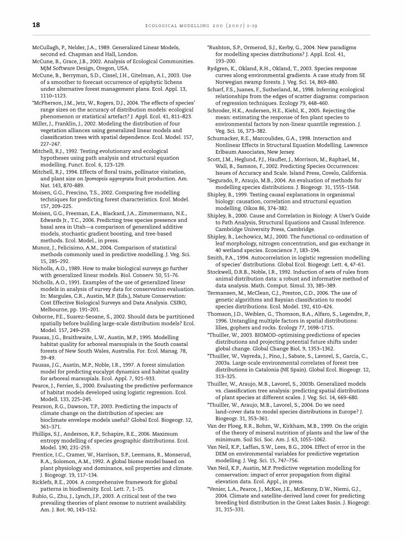
l i n

18 e c o l o g i c a l m o d e l

McCullagh, P., Nelder, J.A., 1989. Generalized Linear Models,second ed. Chapman and Hall, London.

McCune, B., Grace, J.B., 2002. Analysis of Ecological Communities.MjM Software Design, Oregon, USA.

McCune, B., Berryman, S.D., Cissel, J.H., Gitelman, A.I., 2003. Useof a smoother to forecast occurrence of epiphytic lichensunder alternative forest management plans. Ecol. Appl. 13,1110–1123.

*McPherson, J.M., Jetz, W., Rogers, D.J., 2004. The effects of species’range sizes on the accuracy of distribution models: ecologicalphenomenon or statistical artefact? J. Appl. Ecol. 41, 811–823.

Miller, J., Franklin, J., 2002. Modeling the distribution of fourvegetation alliances using generalized linear models andclassification trees with spatial dependence. Ecol. Model. 157,227–247.

Mitchell, R.J., 1992. Testing evolutionary and ecologicalhypotheses using path analysis and structural equationmodelling. Funct. Ecol. 6, 123–129.

Mitchell, R.J., 1994. Effects of floral traits, pollinator visitation,and plant size on Ipomopsis aggregrata fruit production. Am.Nat. 143, 870–889.

Moisen, G.G., Frescino, T.S., 2002. Comparing five modellingtechniques for predicting forest characteristics. Ecol. Model.157, 209–225.

Moisen, G.G., Freeman, E.A., Blackard, J.A., Zimmermann, N.E.,Edwards Jr., T.C., 2006. Predicting tree species presence andbasal area in Utah—a comparison of generalized additivemodels, stochastic gradient boosting, and tree-basedmethods. Ecol. Model., in press.

Munoz, J., Felicisimo, A.M., 2004. Comparison of statisticalmethods commonly used in predictive modelling. J. Veg. Sci.15, 285–292.

Nicholls, A.O., 1989. How to make biological surveys go furtherwith generalized linear models. Biol. Conserv. 50, 51–76.

Nicholls, A.O., 1991. Examples of the use of generalized linearmodels in analysis of survey data for conservation evaluation.In: Margules, C.R., Austin, M.P. (Eds.), Nature Conservation:Cost Effective Biological Surveys and Data Analysis. CSIRO,Melbourne, pp. 191–201.

Osborne, P.E., Suarez-Seoane, S., 2002. Should data be partitionedspatially before building large-scale distribution models? Ecol.Model. 157, 249–259.

Pausas, J.G., Braithwaite, L.W., Austin, M.P., 1995. Modellinghabitat quality for arboreal marsupials in the South coastalforests of New South Wales, Australia. For. Ecol. Manag. 78,39–49.

Pausas, J.G., Austin, M.P., Noble, I.R., 1997. A forest simulationmodel for predicting eucalypt dynamics and habitat qualityfor arboreal marsupials. Ecol. Appl. 7, 921–933.

Pearce, J., Ferrier, S., 2000. Evaluating the predictive performanceof habitat models developed using logistic regression. Ecol.Modell. 133, 225–245.

Pearson, R.G., Dawson, T.P., 2003. Predicting the impacts ofclimate change on the distribution of species: arebioclimate envelope models useful? Global Ecol. Biogeogr. 12,361–371.

Phillips, S.J., Anderson, R.P., Schapire, R.E., 2006. Maximumentropy modelling of species geographic distributions. Ecol.Model. 190, 231–259.

Prentice, I.C., Cramer, W., Harrison, S.P., Leemans, R., Monserud,R.A., Solomon, A.M., 1992. A global biome model based onplant physiology and dominance, soil properties and climate.J. Biogeogr. 19, 117–134.

Ricklefs, R.E., 2004. A comprehensive framework for global

patterns in biodiversity. Ecol. Lett. 7, 1–15.

Rubio, G., Zhu, J., Lynch, J.P., 2003. A critical test of the twoprevailing theories of plant resonse to nutrient availability.Am. J. Bot. 90, 143–152.

g 2 0 0 ( 2 0 0 7 ) 1–19

*Rushton, S.P., Ormerod, S.J., Kerby, G., 2004. New paradigmsfor modelling species distributions? J. Appl. Ecol. 41,193–200.

Rydgren, K., Okland, R.H., Okland, T., 2003. Species responsecurves along environmental gradients. A case study from SENorwegian swamp forests. J. Veg. Sci. 14, 869–880.

Scharf, F.S., Juanes, F., Sutherland, M., 1998. Inferring ecologicalrelationships from the edges of scatter diagrams: comparisonof regression techniques. Ecology 79, 448–460.

Schroder, H.K., Andersen, H.E., Kiehl, K., 2005. Rejecting themean: estimating the response of fen plant species toenvironmental factors by non-linear quantile regression. J.Veg. Sci. 16, 373–382.

Schumacker, R.E., Marcoulides, G.A., 1998. Interaction andNonlinear Effects in Structural Equation Modelling. LawrenceErlbaum Associates, New Jersey.

Scott, J.M., Heglund, P.J., Haufler, J., Morrison, M., Raphael, M.,Wall, B., Samson, F., 2002. Predicting Species Occurrences:Issues of Accuracy and Scale. Island Press, Covelo, California.

*Segurado, P., Araujo, M.B., 2004. An evaluation of methods formodelling species distributions. J. Biogeogr. 31, 1555–1568.

Shipley, B., 1999. Testing causal explanations in organismalbiology: causation, correlation and structural equationmodelling. Oikos 86, 374–382.

Shipley, B., 2000. Cause and Correlation in Biology: A User’s Guideto Path Analysis, Structural Equations and Causal Inference.Cambridge University Press, Cambridge.

Shipley, B., Lechowicz, M.J., 2000. The functional co-ordination ofleaf morphology, nitrogen concentration, and gas exchange in40 wetland species. Ecoscience 7, 183–194.

Smith, P.A., 1994. Autocorrelation in logistic regression modellingof species’ distributions. Global Ecol. Biogeogr. Lett. 4, 47–61.

Stockwell, D.R.B., Noble, I.R., 1992. Induction of sets of rules fromanimal distribution data: a robust and informative method ofdata analysis. Math. Comput. Simul. 33, 385–389.

Termansen, M., McClean, C.J., Preston, C.D., 2006. The use ofgenetic algorithms and Baysian classification to modelspecies distributions. Ecol. Model. 192, 410–424.

Thomson, J.D., Weiblen, G., Thomson, B.A., Alfaro, S., Legendre, P.,1996. Untangling multiple factors in spatial distributions:lilies, gophers and rocks. Ecology 77, 1698–1715.

*Thuiller, W., 2003. BIOMOD-optimising predictions of speciesdistributions and projecting potential future shifts underglobal change. Global Change Biol. 9, 1353–1362.

*Thuiller, W., Vayreda, J., Pino, J., Sabate, S., Lavorel, S., Garcia, C.,2003a. Large-scale environmental correlates of forest treedistributions in Catalonia (NE Spain). Global Ecol. Biogeogr. 12,313–325.

Thuiller, W., Araujo, M.B., Lavorel, S., 2003b. Generalized modelsvs. classification tree analysis: predicting spatial distributionsof plant species at different scales. J. Veg. Sci. 14, 669–680.

*Thuiller, W., Araujo, M.B., Lavorel, S., 2004. Do we needland-cover data to model species distributions in Europe? J.Biogeogr. 31, 353–361.

Van der Ploeg, R.R., Bohm, W., Kirkham, M.B., 1999. On the originof the theory of mineral nutrition of plants and the law of theminimum. Soil Sci. Soc. Am. J. 63, 1055–1062.

Van Neil, K.P., Laffan, S.W., Lees, B.G., 2004. Effect of error in theDEM on environmental variables for predictive vegetationmodelling. J. Veg. Sci. 15, 747–756.

Van Neil, K.P., Austin, M.P. Predictive vegetation modelling forconservation: impact of error propagation from digitalelevation data. Ecol. Appl., in press.

*Venier, L.A., Pearce, J., McKee, J.E., McKenny, D.W., Niemi, G.J.,2004. Climate and satellite-derived land cover for predictingbreeding bird distribution in the Great Lakes Basin. J. Biogeogr.31, 315–331.

i n g

V

W

W

W

W

W

Y

Y

Y

Z

*Johnson, C.J., Seip, D.R., Boyce, M.S., 2004. A quantitativeapproach to conservation planning: using resource selectionfunctions to map the distribution of mountain caribou atmultiple spatial scales. J. Appl. Ecol. 41, 238–251.

e c o l o g i c a l m o d e l l

ile, D., Shipley, B., Garnier, E., 2006. A structural equation modelto integrate changes in functional strategies during old-fieldsuccession. Ecology 87, 504–517.

amelink, G.W.W., Goedhart, P.W., Van Dobben, H.F., Berendse, F.,2005. Plant species as predictors of soil pH: replacing expertjudgement with measurements. J. Veg. Sci. 16, 461–470.

eiher, E., 2003. Species richness along multiple gradients:testing a general multivariate model in oak savannas. Oikos101, 311–316.

eiher, E., Forbes, S., Schauwecker, T., Grace, J.B., 2004.Multivariate control of plant species richness and communitybiomass in blackland prairie. Oikos 106,151–157.

hittaker, R.J., Willis, K.J., Field, R., 2001. Scale and speciesrichness: towards a general, hierarchical theory of speciesdiversity. J. Biogeogr. 28, 453–470.

ood, S.N., Augustin, N.H., 2002. GAMs with integrated modelselection using penalized regression splines and applicationsto environmental modelling. Ecol. Model. 157, 157–178.

ee, T.W., Mackenzie, M., 2002. Vector generalized additivemodels in plant ecology. Ecol. Model. 157, 141–156.

ee, T.W., Mitchell, N.D., 1991. Generalized additive models inplant ecology. J. Veg. Sci. 2, 587–602.

u, K., Jones, M.C., 1998. Local linear quantile regression. J. Am.Stat. Assoc. 93, 228–237.

aneiwski, A.E., Lehmann, A., Overton, J., 2002. Predicting speciesspatial distributions using presence-only data: a case study ofnative New Zealand ferns. Ecol. Model. 157, 261–280.

2 0 0 ( 2 0 0 7 ) 1–19 19

Further reading

*Amar, A., Arroyo, B., Redpath, S., Thirgoods, S., 2004. Habitatpredicts losses of red grouse to individual hen harriers. J.Appl. Ecol. 41, 305–314.

*Cabeza, M., Araujo, M., Wilson, R.J., Thomas, C.D., Cowley, M.J.R.,Moilanen, A., 2004. Combining probabilities of occurrencewith spatial reserve design. J. Appl. Ecol. 41, 252–262.

*Frair, J.L., Nielsen, S.E., Merrill, E.H., Lele, S.R., Boyce, M.S., Munro,R.H.M., Stenhouse, G.B., Beyer, H.L., 2004. Removing GPS collarbias in habitat selection studies. J. Appl. Ecol. 41, 201–212.

*Heikken, R.K., Luoto, M., Virkkala, R., Rainio, K., 2004. Effects ofhabitat cover, landscape structure and spatial variables on theabundance of birds in an agricultural-forest mosaic. J. Appl.Ecol. 41, 824–835.

∗ References used in review in section on current models for pre-dicting species distributions.