Species-Area and Species-Individual Relationships for

Species-Area and Species-Individual Relationships for Tropical Trees: A Comparison of Three50-ha PlotsAuthor(s): Richard Condit, Stephen P. Hubbell, James V. Lafrankie, R. Sukumar, N.Manokaran, Robin B. Foster and Peter S. AshtonReviewed work(s):Source: Journal of Ecology, Vol. 84, No. 4 (Aug., 1996), pp. 549-562Published by: British Ecological SocietyStable URL: http://www.jstor.org/stable/2261477 .

Accessed: 10/12/2012 15:34

Your use of the JSTOR archive indicates your acceptance of the Terms & Conditions of Use, available at .http://www.jstor.org/page/info/about/policies/terms.jsp

.JSTOR is a not-for-profit service that helps scholars, researchers, and students discover, use, and build upon a wide range ofcontent in a trusted digital archive. We use information technology and tools to increase productivity and facilitate new formsof scholarship. For more information about JSTOR, please contact [email protected].

.

British Ecological Society is collaborating with JSTOR to digitize, preserve and extend access to Journal ofEcology.

http://www.jstor.org

This content downloaded by the authorized user from 192.168.52.67 on Mon, 10 Dec 2012 15:34:27 PMAll use subject to JSTOR Terms and Conditions

http://www.jstor.org/action/showPublisher?publisherCode=briteco

http://www.jstor.org/stable/2261477?origin=JSTOR-pdf

http://www.jstor.org/page/info/about/policies/terms.jsp


Journal of Ecology 1996, 84, 549-562

Species-area and species-individual relationships for tropical trees: a comparison of three 50-ha plots RICHARD CONDIT, 'STEPHEN P. HUBBELL, 1'2

JAMES V. LAFRANKIE,3 R. SUKUMAR,4 N. MANOKARAN,s ROBIN B. FOSTER1'6 and PETER S. ASHTON7 'Center for Tropical Forest Science, Smithsonian Tropical Research Institute, Unit 0948, APO AA 34002-0948, USA, 2Department of Ecology and Evolutionary Biology, Princeton University, Princeton, NJ 08544, USA, 3Center for Tropical Forest Science, National Institute of Education, 469 Bukit Timah Road, Singapore 1025, 4Centre for Ecological Sciences, Indian Institute of Science, Bangalore, 560012, India, 'Forest Research Institute of Malaysia, Kepong, 52109 Kuala Lumpur, Malaysia, 6Department of Botany, Field Museum of Natural History, Chicago, IL 60605 USA and 7Harvard Institute for International Development and Arnold Arboretum, One Eliot Street, Cambridge, MA 02138, USA

Summary

1 Species-accumulation curves for woody plants were calculated in three tropical forests, based on fully mapped 50-ha plots in wet, old-growth forest in Peninsular Malaysia, in moist, old-growth forest in central Panama, and in dry, previously logged forest in southern India. A total of 610000 stems were identified to species and mapped to < 1 m accuracy. Mean species number and stem number were calculated in quadrats as small as 5 m x 5 m to as large as 1000 m x 500 m, for a variety of stem sizes above 10 mm in diameter. Species-area curves were generated by plotting species number as a function of quadrat size; species-individual curves were generated from the same data, but using stem number as the independent variable rather than area. 2 Species-area curves had different forms for stems of different diameters, but species-individual curves were nearly independent of diameter class. With < 104 stems, species-individual curves were concave downward on log-log plots, with curves from different forests diverging, but beyond about 104 stems, the log-log curves became nearly linear, with all three sites having a similar slope. This indicates an asymptotic difference in richness between forests: the Malaysian site had 2.7 times as many species as Panama, which in turn was 3.3 times as rich as India. 3 Other details of the species-accumulation relationship were remarkably similar between the three sites. Rectangular quadrats had 5-27% more species than square quadrats of the same area, with longer and narrower quadrats increasingly diverse. Random samples of stems drawn from the entire 50 ha had 10-30% more species than square quadrats with the same number of stems. At both Pasoh and BCI, but not Mudumalai, species richness was slightly higher among intermediate-sized stems (50-100 mm in diameter) than in either smaller or larger sizes. These patterns reflect aggregated distributions of individual species, plus weak density-dependent forces that tend to smooth the species abundance distribution and 'loosen' aggregations as stems grow. 4 The results provide support for the view that within each tree community, many species have their abundance and distribution guided more by random drift than deterministic interactions. The drift model predicts that the species-accumulation curve will have a declining slope on a log-log plot, reaching a slope of 0.1 in about 50 ha. No other model of community structure can make such a precise prediction. 5 The results demonstrate that diversity studies based on different stem diameters can be compared by sampling identical numbers of stems. Moreover, they indicate that stem counts < 1000 in tropical forests will underestimate the percentage difference in species richness between two diverse sites. Fortunately, standard diversity indices (Fisher's oc, Shannon-Wiener) captured diversity differences in small stem samples more effectively than raw species richness, but both were sample size dependent. Two nonparametric richness estimators (Chao, jackknife) performed poorly, greatly underestimating true species richness.

Keywords: diversity, tropical forest, species-area curve, species-individual curve

Journal of Ecology (1996) 84, 549-562 c 1996 British Ecological Society



550 Species-area in tropical forests

Introduction

Species-area and species-individual curves have been central to community ecology for decades (Fisher et al. 1943; Preston 1948, 1962; MacArthur & Wilson 1967). They are a fundamental component of conservation biology and are frequently used to for- mulate recommendations about species preservation and to predict extinction rates caused by habitat destruction (Diamond 1975; Schafer 1990; Pimm et al. 1995). Despite widespread attention from field ecologists and mathematical biologists, species-area analysis is largely empirical: the theoretical basis of the species-area curve is not well understood (Sim- berloff 1976; Angermeier & Schlosser 1989; Kelly et al. 1989; Kohn & Walsh 1994; Hubbell 1995, in press). Even the empirical form of species-area and species- individual relationships is debated at length (Connor & McCoy 1979).

Trees are a useful subject for analyses of such relationships, because they are easy to locate precisely and to count, and tropical trees are an especially interesting subject because they are so diverse. Many studies of local diversity of tropical trees exist, and there is a great deal of interest in patterns and processes relating to tropical forest diversity (Gentry 1988; Wright 1992; Phillips et al. 1994; Phillips & Gentry 1994; Valencia et al. 1994; Condit 1995). Nevertheless, there are few detailed analyses of species-area and species-individual relationships from tropical forests.

Here we present a thorough documentation of how species richness increases with the area censused or with the number of trees censused, using data from three 50-ha plots in three different forest types. One plot is in aseasonal, highly diverse forest in peninsular Malaysia (Manokaran et al. 1992), the second in seasonal, moderately diverse forest in Panama (Hubbell & Foster 1983; Condit et al. 1992b), and the third in seasonal, dry, low-diversity forest in southern India (Sukumar et al. 1992). Each plot was censused in exactly the same way: a 1-km x 0.5-km region was mapped, and all trees > 10 mm in stem diameter were identified and precisely located within it. The plots form part of an international network of 12 large-scale forest dynamics plots now under- way (Condit 1995). With this unique database, we seek general answers about species-area patterns of tropical forests. What is the form of the species- area and species-individual relationship? How does it change when different stem sizes are included? Does the shape of a quadrat affect the number of species found within, given constant area? Does the number of individuals within a constant area affect the number of species? And, most generally, what theories of community structure are consistent with observed species-accumulation patterns?

Materials and methods

STUDY SITES

The plot in Malaysia is in the Pasoh Forest Reserve in the centre of the Malay peninsula, 140 km south- east of Kuala Lumpur. The reserve is a 2000-ha rem- nant of old-growth forest connected to a larger pro- duction forest, dominated by Dipterocarpaceae and classified as red meranti-keruing by Wyatt-Smith (1987). Rainfall is 2000mm per year and relatively aseasonal, with every month averaging more than 100 mm (Kochummen et al. 1990). The canopy is ever- green. The forest is on level terrain, with topographic variation of 25 m in 50 ha. There are 817 species and 335000 stems > 1Omm in diameter in the 50-ha plot (Manokaran et al. 1992).

The plot on Barro Colorado Island in the Panama Canal is also in rich, old-growth tropical forest (except for two of the 50 ha, which were cleared < 100 years ago), dominated by Leguminosae and Bombacaceae. Rainfall is highly seasonal, with a strong 4-month dry season from December through April, but the yearly total of 2500 mm exceeds that at Pasoh (Leigh et al. 1982). About 18% of the canopy is deciduous (Condit et al. 1996). The 50-ha plot is on mainly level terrain on the island's summit, with 28 m of vertical variation. The forest at BCI is structurally quite like the one at Pasoh, with 244 000 stems > 0mm in diameter in 50 ha, but there are only 303 species in the plot (Con- dit et al. 1992b).

The third plot is in the Mudumalai Game Reserve in the state of Tamil Nadu, about 250 km south-west of Bangalore, India (Sukumar et al. 1992). This is a dry, deciduous forest, dominated by teak (Tectona grandis, Verbenaceae), Lythraceae, and Combre- taceae, and was subjected to logging until the 1960s. Rainfall is 1200 mm per year, with a December-May dry season during which most canopy trees lose their leaves. The reserve is on a rolling plateau just north of the Nilgiri Hills, and topographic variation within the plot is 129 m. Structurally, the forest at Mud- umalai is very different from the other two 50-ha plots: there are just 26 000 stems in 50 ha, and grasses dominate the understorey, but large trees form a nearly complete canopy. Fires are common, and elephants play a major role as browsers on young trees and shrubs. There are only 71 species in 50 ha, less than one-tenth the richness at Pasoh.

CENSUS METHODS

All free-standing, woody stems > 10mm diameter at breast height (d.b.h.) were identified, tagged, and mapped o t he nearest metre (Hubbell & Foster 1983; Manokaran et al. 1990; Sukumar et al. 1992; Condit et al. 1995). The diameter of each stem was measured 1.3 m above the ground unless there were irregularities

c 1996 British Ecological Society, Journal of Ecology, 84, 549-562



551 Richard Condit et al.

in the trunk there, in which case the measurement was taken at the nearest lower point where the stem was cylindrical, or above the buttresses on large trunks. Diameters at breast height were measured with cal- lipers and recorded to the nearest millimetre. Trees with multiple stems connected near the ground were counted as single individuals and assigned the d.b.h. of the largest stem (d.b.h. of the secondary stems was recorded but not used in this analysis). The Pasoh 50- ha plot was fully censused from 1986 to 1989, then again in 1990; we use data from the first census here. BCI censuses were carried out in 1981-83, 1985, 1990 and 1995 (Hubbell & Foster 1983, 1986, 1992; Condit et al. 1992a,b); here we use 1990 data. Mudumalai was censused completely in 1987 and 1991; we use 1987 data here.

SPECIES-AREA CURVES

To generate species-area curves, the entire 50-ha plot was divided into nonoverlapping square or rectangular quadrats, and the number of species present in each tallied. For example, the plot can be split into 1250 20-m x 20-m quadrats. Square quadrats of the following dimensions were used: 5, 10, 20, 25, 31.6 (to give 0.1 ha), 40, 50, 100, 150, 200, 250 and 500m. In cases where the dimension of the whole plot (500 m x 1000 m) did not divide evenly into the size of the quadrat, the northern edge or eastern edge of the plot was left out. For example, with 150-m x 150-m quadrats, only 450 m x 900 m of the plot could be used, so the northern 50 m and the eastern lOOm were omitted. The mean number of species in each size quadrat gave a species-area curve for square quadrats. The same approach was used for rectangular quadrats: we divided the plot into adjacent, nonoverlapping rectangles of 200m x 2m, 400m x 4m, 500m x 5m and lOOOm x lOm, thus maintaining a constant shape, plus 500m x 20m, lOOOm x 1 m, and lOOOm x 500m (full plot); in each, the long dimension was parallel to the 1000-m axis of the full plot. Long, thin quadrats were chosen to contrast with squares and to match the shape of frequently used transects (Boom 1986; Gentry 1988).

SPECIES-INDIVIDUAL CURVES

Species-individual curves were constructed exactly as were species-area curves, but instead of area on the horizontal axis we used the mean number of individuals in quadrats of each area. We also evaluated species-individual curves within quadrats of a single area, for example, species number vs. stem number from the 50 one-hectare squares. This was repeated for square quadrats 20, 25, 40 and 50 m on a side, and regressions of species number vs. the logarithm of individual number performed. This was done for stems ?> 10 mm d.b.h. but not the other d.b.h. classes (see d.b.h. classes).

Species-individual curves were also extended to areas much larger than 50 ha, based on available species counts in regional floras. There are an estimated 3197 species of trees and shrubs in the 131 000 km2 of Peninsular Malaysia (Kochummen et al. 1992). On BCI, Croat (1978) lists 450 species of trees and shrubs, and we found a further 17 in the 50-ha plot. In the Panama Canal Area, with 1259 km2 of land, there are 855 native trees and shrubs, while in the entire nation of Panama, with 77000km2, there are 2870 species (these are based on the computerized flora of Panama released by the Missouri Botanical Garden (see D'Arcy 1987a,b), updated by R.B.F.). At Mudumalai, one of us (R.S.) counted 229 tree and shrub species in the plant checklist, which covers the 32 100-ha sanctuary. To estimate the number of individuals in the larger areas, we applied the density of plants > 10 mm d.b.h. within the 50-ha plots, thus assuming that the entire region was covered with forest of similar structure and also assuming that counts of 'trees and shrubs' include all species >? 10mm d.b.h. Obviously, these estimates are crude, but slopes on a double-log plot are not that sensitive to moderate errors. We calculated log-log slopes for species-individual curves using adjacent points - successively larger samples - on the graphs.

COMPARISON TO OTHER METHODS

There are two main approaches to constructing species-area curves which differ in the order in which quadrats (or individuals) are accumulated (Palmer 1990). One is to use a nested series of expanding quadrats. With this approach, geographical integrity is maintained, since quadrats are added in geographical order (the order is obvious in a linear series of quadrats, less obvious but still definable in a rectangular plot). A large number of nested series can be recalculated from one dataset, starting from a different point each time, to yield a mean accumulation curve. Our approach is effectively identical to this, since we calculated the number of species in rectangular quadrats of expanding size. Our technique is much easier, though, and it fully samples the plots while avoiding nonindependence of repeated curves (multiple random nested series might have partially overlapping quadrats of a given area; in our method, quadrats of a given area never overlap).

The alternative approach is to add individuals or quadrats in random order from across the whole plot (Palmer 1990; Colwell & Coddington 1994). Geo- graphical integrity is lost, since the second quadrat (or individual) added may be far away from the first. Fortunately, it is possible to calculate analytically a curve based on random stem order, so it is not necess- ary to use a sampling approach. We describe this method below as the Hurlbert (1971) formulation of 'expected species number'. The alternative of randomizing quadrat order maintains geographical

C 1996 British Ecological Society, Journal of Ecology, 84, 549-562




integrity within the smallest quadrat area but loses integrity at larger areas.

There are drawbacks to the randomization approach. Most importantly, the species-accumulation curve will depend on the size of the area sampled, and thus is not comparable across sites. For example, with a 1-ha plot at one site and a 10-ha plot at another, a curve based on the nested approach from the former would be strictly comparable to the first hectare of a curve from the latter site; this would not be true of the randomization approach. The second drawback is that the randomization method does not actually report the number of species present in a given contiguous area, instead, it gives the number of species found in small, scattered quadrats, which is not a very useful number. The method we use here reports the actual average of species counts within quadrats of various sizes.

D.B.H. CLASSES

Species-area and species-individual curves were calculated separately for all stems > each of the following d.b.h. cut-offs: 10mm (all stems in each census), 20, 25, 31.8 (giving a circumference of 100 mm), 50, 100, 200, 300, 400 and 600 mm. These cut-offs were designed to match most other forest surveys, allowing direct comparisons. These are overlapping classes, that is, individuals > 100 mm d.b.h. are included within the group > 10mm d.b.h. This approach was chosen to permit direct comparison with other studies of tropical forest, which nearly always count all stems above one of these limits. It has the drawback, however, that the d.b.h. classes are not independent of one another. Thus, in order to compare species diversity in different d.b.h. classes, we repeated calculations using nonoverlapping d.b.h. classes: 10-29, 30-49, 50-69, 70-99, 100-149, 150- 199, 200-299, 300-499 and > 500 mm.

INDICES OF DIVERSITY

We calculated four commonly used indices of diversity: Fisher's oc, Simpson's index, the Shannon-Wiener index, and the index of dominance. Fisher's oc is defined by

S =c(+ IY) (1)

where S = species number, N = individual number, ln means the natural logarithm, and oc is the sole parameter (Fisher et al. 1943). An estimate of oc can be made for any pair of S and N using Newton's method (Condit et al. in press). Simpson's index is given by

EZN (2)

where J; is the relative abundance of species i (Simpson 1949; Kempton 1979). The Shannon-Wiener index is

Z-(flnf) (3)

(Pielou 1966, 1975; Kempton 1979). The dominance index is the largestf, or the relative abundance of the most numerous species in a quadrat (Berger & Parker 1970). All indices were calculated for each individual quadrat.

In addition, we tested two more recently developed nonparametric' indices, the Chao and the second- order jackknife estimators of species richness (Helts- che & Forrester 1983; Chao 1984; Colwell & Codding- ton 1994). In contrast to the four indices listed above, these are not arbitrary metrics of diversity but are supposed to yield estimates of total species richness. The Chao index C is given by

C= (S+(S) (4)

and the jackknife index J by

J = S+{ S(2N 3 )- S2(N 2

)2} (5) J= ~?s~~N N(N-1)}

where S1 is the total number of species represented by a single individual, S2 by two individuals, and S and N as defined above. (Si and S2 can alternatively rep- resent the number of species found in one subsample and two subsamples, respectively, of a larger sample. We tested this alternative by defining subsamples as 5-m x 5-m, 10-m x 10-m or 20-m x 20-m subqua- drats of larger quadrats and found estimates nearly identical to those given by eqns 4 and 5; we report on just the latter.)

EXPECTED NUMBER OF SPECIES

We also make use of a formulation for the 'expected' number of species in a subsample of individuals drawn from a larger known sample; in our study, the larger sample was the entire 50-ha plot. This is equivalent to randomizing the order in which individuals are added in a species-individual curve. Given a set of abundances N, for S species, and N = X,N,, the number of species s in a subsample of n plants taken at random from the larger sample is

s = Eip,(N,, N, n) (6)

where p,(N,,N,n) is the probability of encountering species i in the subsample (Hurlbert 1971). This probability is found from a hypergeometric formulation,

p,(N,, N, n) = 1- UN( N;) (c 1996 British Ecological Society, Journal of Ecology, 84, 549-562




Hubbell & Foster (1983, 1992) made analogous calculations for the number of species expected in small areas within the BCI 50-ha plot. This s illustrates the impact of contagion on the species-accumulation curve, since s will equal S from a subregion only if species are randomly intermingled (Hubbell & Foster 1992).

SPECIES PER FIXED INDIVIDUAL COUNT

To compare species richness and estimators of diversity between d.b.h. classes or between plots, we needed estimates from precisely the same numbers of individuals. We generated these by simple linear interpolation on semilog plots, i.e., richness or diversity indices vs. the logarithm of the number of individuals. For example, to calculate species richness in exactly 500 individuals > 10mm d.b.h. at BCI, we plotted mean species number vs. the logarithm of mean individual number for all quadrat sizes from 5-m x 5-m to 500-m x 500-m, connected the points with lines, and then read off the value at 500 plants. Semilog plots were most appropriate because they were either straight lines or slowly bending curves across a wide range of individuals for all indices.

Results

SPECIES-AREA CURVES

The form of the species-area curve from all three forests was similar. On semilog plots, curves were nearly linear for stems > 10mm d.b.h., but concave upward for larger d.b.h. classes. On log-log plots (Fig. 1), species-area curves were concave downward, but curves from different d.b.h. classes were not parallel. They converged as area increased, reflecting an increase in the proportion of total species that fell in the larger d.b.h. classes with increasing area. For example, at BCI, in 20-m x 20-m quadrats (0.04 ha), less than a quarter of the species were > 100 mm (12 species > 100mm d.b.h. and 54 species > 10mm), compared with nearly 60% (163 of 280) in 25 ha quadrats. The pattern was similar at Pasoh (Fig. 1). At Mudumalai, the curves also converged, but not nearly as much: even in the smallest quadrats, most species were > 100mm d.b.h. Tables 1-3 give full datasets on species number in different areas and different d.b.h. classes in all three plots.

SPECIES-INDIVIDUAL CURVES

In contrast, when species number was plotted against the number of individuals, different d.b.h. classes fell on nearly identical curves. That is, in all three forests, the number of species in a given number of individuals was nearly independent of d.b.h. class. On semilog plots, species-individual curves were concave upward for < 500 stems, then became linear; at Pasoh and

0.1 1 10 1000

1asoh - , . . . . . - - - - -.-.-.-,-.-.-

1(0 0 -

Pao - - . - - ---------- --21-0

* , '?100

BCI----- --0

....... ...3........00

10-~~~~~~~~~~~~~~>1

10 .

0.1 1 10

area

Fig. 1 Species-area curves from three 50-ha plots, three different d.b.h. classes at each, plotted on log-log scales. Vertical bars show 95% confidence limits for species number; when not visible, confidence limits were too small to show up on the graph. All points are from square quadrats except the right-most, which are from the entire 1000Om x 500Om (the latter do not have confidence limits).

Mudumalai, they became slightly concave downward in the largest samples (Fig. 2). On log-log plots, the curves were concave downward (Fig. 3), with essentially the same form in all three forests.

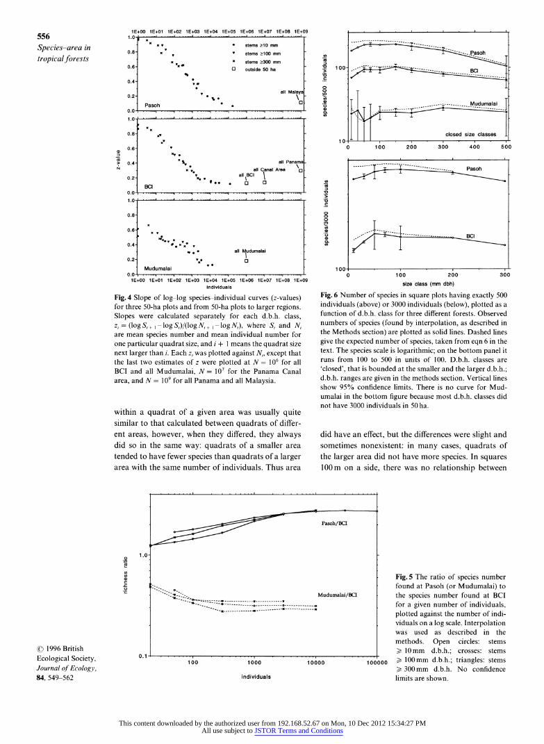
The slope of the log-log species-individual curves (the 'z-value') declined with individual number in all three plots, reaching a value of around 0.10 in the largest samples (Fig. 4). At Pasoh, the slope from 50ha to the entire Malay Peninsula was 0.11. In Panama, z was 0.13 from 50 ha to 1500 ha (all Barro Colorado Island) and from there to the entire Canal Area (Fig. 4), while it was 0.29 from the Canal Area to the rest of Panama. In India, z = 0.17 from 50 ha to the 32 000 ha in Mudumalai (Fig. 4).

DIVERSITY DIFFERENCES BETWEEN FORESTS

In samples > 3000 individuals, the Pasoh forest con- sistently had 2.7 times as many species as BCI (Fig. 5). In smaller samples, the diffeience was less, and in samples of < 10 individuals, the forests were barely different. Comparing BCI and Mudumalai, the difference in species richness reached a plateau at about 300 individuals, with Mudumalai 0.3 times as rich as BCI. To compare Pasoh and Mudumalai, one would divide the value from the top curve by the value from the bottom in Fig. 5; this would reach an

c) 1996 British Ecological Society, Journal of Ecology, 84, 549-562



Table 1 Means and 95% confidence intervals for species number in the Pasoh 50-ha plot (confidence limits were calculated with a t-statistic). The largest quadrat, 1000 m x 500 m, is the entire plot, so there were no replicates and thus no confidence limits. The mean number of stems for any quadrat size can be calculated from the mean density per ha over the whole plot: 6702.0 for stems ? 10 mm d.b.h., 3879.1 for stems > 20 mm, 2566.2 for stems ) 25.4 mm, 2123.8 for stems ? 31.8 mm, 1371.6 for stems > 50 mm, 529.0 for stems > 100 mm, 168.1 for stems ? 200 mm, 75.4 for stems ? 300 mm, 40.3 for stems >? 400 mm, and 14.3 for stems ? 600 mm. The actual number of stems for 40-m x 40-m and 150-m x 150-m plots were slightly different, because these quadrat dimensions did not cover the entire 50 ha

Size class (mm d.b.h.) Quadrat size (m) ?10 ?20 ?25.4 ?31.8 ?50 ?100 ?200 ?300 ? 400 > 600

20 x 20 126.8+0.8 91.8+0.6 69.8+0.5 60.9+0.4 43.2+0.3 18.8+0.2 6.3+0.1 2.9+0.1 1.6+0.1 0.6+0.0 25 x 25 166.9+ 1.1 124.4+0.9 96.9+0.7 85.5+0.6 62.0+0.5 28.0+0.3 9.6+0.2 4.4+0.1 2.4+0.1 0.9+0.1 40 x 40 267.3+2.0 213.1+1.6 175.5+1.4 159.1+1.4 122.9+1.2 61.0+0.8 22.5+0.5 10.6?0.3 5.8?0.3 2.1+0.2 50 x 50 323.0+2.7 265.1+2.3 223.5+2.1 205.1+2.0 163.3+ 1.7 85.5+ 1.3 32.7+0.8 15.6+0.5 8.6+0.4 3.2+0.2 100 x 100 494.5+6.2 438.1 +6.2 395.3+6.0 375.6+6.0 326.8+5.7 205.9+4.8 92.1 +3.7 46.3+2.3 26.2+ 1.6 9.9+0.8 150 x 150 581.4+10.8 531.2+12.9 493.6+12.4 475.9+12.6 429.9+12.1 303.9+12.9 151.1+9.9 79.6+7.3 45.6+4.5 17.9+2.6 200 x 200 634.6+12.3 588.5+16.7 551.8+18.6 536.1+18.9 498.4+16.9 374.0+16.7 204.3+15.2 113.2+11.4 65.9+7.1 26.3+3.6 250 x 250 681.4+ 15.9 638.8+23.0 606.9+26.2 592.0+27.0 557.5+22.3 441.4+23.2 260.3+23.6 147.9+ 18.5 85.8+ 10.6 34.3+6.6 500 x 500 782.0+3.9 754.0+0.0 732.0+ 17.3 722.5+ 15.2 694.5+ 10.8 607.5+2.9 441.5+8.8 293.0+34.6 181.5+28.4 75.5+23.8 1000 x 1 256.4+ 1.1 194.1+1.0 153.2?0.9 136.0+0.8 99.6?0.8 45.4?0.6 15.6?0.3 7.1 ?0.2 3.9?0.2 1.4?0.1 500 x 2 245.1? 1.3 186.4?1.1 147.7?0.9 131.4+0.9 97.0?0.8 44.6?0.6 15.4?0.3 7.1 ?0.2 3.8?0.2 1.4?0.1 200 x 2 139.6+0.7 99.4?0.5 74.7?0.4 64.8+0.4 45.4?0.3 19.4?0.2 6.4?0.1 2.9+0.1 1.6?0.1 0.6?0.0 400 x 4 297.0+2.1 234.4? 1.7 192.2? 1.4 173.6? 1.3 132.6? 1.2 64.8?0.9 23.2?0.6 10.8+0.4 5.9?0.3 2.1?0.2 500 x 5 357.9?2.6 292.8?2.3 246.4?2.1 225.6? 1.9 178.1? 1.6 92.0? 1.2 34.4?0.8 16.2?0.5 8.9?0.4 3.4?0.3 1000 x 10 544.5?5.3 484.0+5.2 438.5?5.1 416.2?5.2 361.6?5.1 226.9+4.3 100.6?3.2 50.1? 1.8 28.3? 1.2 11.0?0.9 500 x 20 520.9?6.0 464.0?6.6 420.0+6.2 398.3?6.1 346.2+5.6 218.2?4.6 97.3?3.2 48.3?2.1 27.0? 1.5 10.5? 1.0 1000 x 500 817 799 781 773 752 683 525 377 248 102

Table 2 Means and 95% confidence intervals for species number in the Barro Colorado Island 50-ha plot (confidence limits were calculated with a t-statistic). The largest quadrat, 1000 x 500 m, is the entire plot, so there were no replicates and thus no confidence limits. The mean number of stems for any quadrat size can be calculated from the mean density per ha over the whole plot: 4881.8 for stems > 10 mm d.b.h., 2885.6 for stems ? 20 mm, 2201.1 for stems > 25.4 mm, 1740.4 for stems > 31.8 mm, 1022.4 for stems > 50mm, 424.8 for stems > 100mm, 155.1 for stems ? 200mm, 82.4 for stems > 300mm, 47.2 for stems > 400mm, and 17.3 for stems > 600mm. The actual number of stems for 40-m x 40-m and 1 50-m x 1 50-m plots were slightly different, because these quadrat dimensions did not cover the entire 50 ha

Size class (mm d.b.h.) Quadrat size (m) >10 ?20 ?25.4 > 31.8 > 50 > 100 > 200 ?300 > 400 > 600

20 x 20 53.7?0.5 42.6?0.4 37.4?0.4 33.1 ?0.4 23.7+0.3 12.5?0.2 5.3?0.1 3.0?0.1 1.8?0.1 0.7?0.0 25 x 25 67.4?0.7 54.9+0.6 49.0+0.6 43.8?0.5 32.3?0.4 17.7?0.3 7.7?0.2 4.4?0.1 2.7?0.1 1.0?0.1 40 x 40 100.6? 1.2 86.6+ 1.1 79.6+ 1.1 73.3? 1.1 57.5? 1.0 34.1 +0.6 16.4?0.4 9.9?0.3 6.2?0.2 2.5?0.2 50 x 50 117.8? 1.4 104.1? 1.4 96.9? 1.3 90.3? 1.3 72.9? 1.2 44.9+0.8 22.7?0.5 13.8?0.4 8.8?0.4 3.7?0.2 100 x 100 172.4?2.4 160.2?2.4 153.0?2.3 147.3?2.2 128.7+2.4 91.2? 1.9 53.6? 1.2 35.2+ 1.4 24.1? 1.1 11.2?0.9 150 x 150 200.6?3.9 190.7?3.8 184.2?3.8 178.4+3.9 162.6+3.4 123.5?3.6 78.0+2.5 54.4?2.5 38.2?2.0 20.2?2.3 200 x 200 219.3?5.9 208.9?5.7 203.9?6.1 199.4?5.7 184.0?4.9 145.8?5.2 99.2?4.9 70.0?4.0 51.2?3.0 28.7?3.3

250 x 250 232.9?6.5 222.6?6.1 217.8?7.2 213.4?7.3 200.6?7.0 162.8+5.6 116.0?6.1 83.8?5.2 61.1 ?4.8 35.6?5.4 500 x 500 279.5+2.9 265.5? 10.8 261.5+ 15.2 259.5? 19.5 242.5? 1.0 208.0?3.9 163.0?2.0 127.5?6.5 95.5? 1.0 59.5? 10.8 1000 x 1 98.3?0.6 82.3?0.6 74.0?0.6 66.8?0.5 50.0?0.5 28.1 ?0.4 12.4?0.3 7.1 ?0.2 4.3?0.2 1.7?0.1

500 x 2 94.3?0.6 78.8?0.6 71.0?0.6 64.1 +0.6 48.5?0.5 27.4?0.4 12.2+0.3 7.1 +0.2 4.3?0.2 1.7?0.1 200 x 2 58.8?0.4 46.3?0.4 40.4?0.3 35.4+0.3 25.1 ?0.3 13.2?0.2 5.5?0.1 3.1 ?0.1 1.8?0.1 0.7+0.1 400 x 4 109.2+ 1.1 94.3+ 1.0 86.7? 1.0 79.8?0.9 62.7?0.9 36.8+0.6 17.2?0.4 10.2?0.3 6.3?0.3 2.5+0.2 500 x 5 129.5? 1.1 114.3? 1.1 106.2? 1.0 98.9? 1.0 80.0? 1.0 49.2+0.7 24.3?0.5 14.8?0.4 9.6?0.4 3.9+0.2 1000 x 10 189.0?2.0 175.4? 1.9 168.2? 1.8 161.6? 1.6 142.4? 1.7 100.2? 1.6 58.4? 1.2 38.9? 1.1 26.5?0.9 12.7?0.8

500 x 20 180.8?2.3 168.3?2.1 161.4?2.1 155.1?2.2 136.1 ?2.3 96.0?1.7 55.9? 1.3 37.3+1.1 25.5+1.0 12.0?0.7 1000 x 500 303 291 287 284 269 229 181 146 112 69

asymptote at about 104 stems, with Pasoh 9.0 times richer than Mudumalai.

SPECIES-INDIVIDUAL CURVES FOR DIFFERENT

D.B.H. CLASSES

Species-accumulation curves from nonoverlapping (and thus independent) d.b.h. classes were identical in form to those in Figs 1-3, and are not shown. Instead, we focus on the number of species in a fixed number of individuals in each d.b.h. class (Fig. 6). For BCI and Pasoh, richness peaked at d.b.h. 50-150mm. At

Mudumalai, though, the curves were essentially flat across all values of d.b.h.

SPECIES-INDIVIDUAL CURVES FOR CONSTANT

AREA

Within square quadrats of 20, 25, 40 and 50 m on a side, species number correlated strongly with individual number in all three forests (P < 0.01 for regressions of species number vs. the logarithm of individual number, all four quadrat sizes in all three plots). The slope of the species-individual curve

(c 1996 British Ecological Society, Journal of Ecology, 84, 549-562



Table 3 Means and 95% confidence intervals for species number in the Mudumalai 50-ha plot (confidence limits were calculated with a t-statistic). The largest quadrat, 1000 x 500 m, is the entire plot, so there were no replicates and thus no confidence limits. The mean number of stems for any quadrat size can be calculated from the mean density per ha over the whole plot: 513.8 for stems > 10mm d.b.h., 472.1 for stems > 20 mm, 451.4 for stems > 25.4 mm, 443.0 for stems ? 31.8 mm, 412.3 for stems > 50 mm, 300.8 for stems > 100 mm, 177.4 for stems > 200 mm, 97.6 for stems > 300 mm, 53.7 for stems > 400 mm, and 11.2 for stems > 600 mm. The actual number of stems for 40-m x 40-m and 150-m x 150-m plots were slightly different, because these quadrat dimensions did not cover the entire 50 ha

Size class (mm d.b.h.) Quadrat size (m) > 10 ?20 ?25.4 ?31.8 ?50 100 ?200 ?300 ?400 600

20 x 20 6.8+0.1 6.4+0.1 6.2+0.1 6.1+0.1 5.9+0.1 5.2+0.1 4.0+0.1 2.7+0.1 1.7+0.1 0.4+0.0 25 x 25 8.6+0.2 8.1 +0.2 7.8 +0.2 7.8 +0.2 7.5 +0.2 6.7+0.1 5.2+0.1 3.6+0.1 2.3 +0.1 0.6+0.1 40 x 40 13.1+0.3 12.5+0.3 12.2+0.3 12.1 +0.3 11.8+0.3 10.5+0.3 8.4+0.2 6.1+0.2 4.1+0.2 1.4+0.1 50 x 50 15.6+0.5 15.0+0.4 14.6+0.4 14.5+0.4 14.1+0.4 12.7+0.4 10.3+0.3 7.5+0.3 5.2+0.3 1.9+0.2 100 x 100 26.2+1.3 25.3+1.2 24.8+1.1 24.6+1.1 24.1+1.0 22.1 +0.8 18.3+0.6 14.3+0.7 10.0+0.8 4.6+0.7 150 x 150 37.1+2.1 35.7+1.9 35.0+1.8 34.8+1.8 34.0+1.6 31.7+1.4 25.8+1.2 20.6+1.3 14.8+1.3 7.6+1.2 200 x 200 43.9+3.9 42.4+4.1 41.3+3.7 41.0+3.7 40.4+2.8 37.6+2.3 31.2+ 1.1 25.8+2.1 18.7+2.1 9.9+ 1.8 250 x 250 49.9+3.3 47.9+3.8 47.0+3.7 46.8+3.8 46.0+2.7 44.1 + 1.9 36.6+ 1.5 30.8+ 1.6 23.5+2.0 12.4+ 1.6 500 x 500 65.0+3.9 63.5+ 10.8 62.0+ 13.0 61.0+ 17.3 60.5?6.9 58.0?2.0 53.5?2.9 46.5?2.2 40.0?0.0 19.5?2.2 1000 x 1 13.7?0.2 13.0?0.2 12.6?0.2 12.5?0.2 12.1?0.2 10.4?0.2 7.8?0.2 5.3?0.1 3.3+0.1 1.0?0.1 500 x 2 13.1 ?0.2 12.5?0.2 12.1 ?0.2 12.0?0.2 11.6?0.2 10.1?0.2 7.6?0.2 5.2?0.2 3.3?0.1 1.0?0.1 200 x 2 7.9+0.1 7.4?0.1 7.2?0.1 7.1 ?0.1 6.8?0.1 5.8?0.1 4.3+0.1 2.8?0.1 1.7?0.1 0.4+0.0 400 x 4 15.8 ? 0.3 15.0 ?0.3 14.6 +0.3 14.4 +0.3 14.0 ?0.3 12.2 ?0.3 9.3 +0.2 6.5 ?0.2 4.4 ?0.2 1.5 +0.1 500 x 5 18.6?0.4 17.8?0.4 17.4+0.3 17.2+0.3 16.8?0.3 14.8?0.3 11.6+0.3 8.4?0.3 5.6?0.2 2.1 ?0.2 1000 x 10 31.6?0.9 30.1 +0.9 29.5+0.9 29.2?0.8 28.7?0.8 26.0?0.8 21.5?0.7 16.5?0.8 11.5?0.7 5.3?0.5 500 x 20 29.6? 1.0 28.4? 1.0 27.8?0.9 27.6?0.8 27.0?0.8 24.6?0.7 20.3+0.7 15.7?0.7 11.2+0.7 5.2+0.5 1000 x 500 71 69 67 67 66 63 59 52 45 25

800 - - Pasoh

Ay

600 -

400- --

200-

0 1 E+00 1 E+01 1 E+02 1 E+03 1 E+04 1 E+05

3007 BCI

2007 20. --'- ?100

C 100 00 ... ?300 A

0 . N**- ..... , 1 E+00 1 E+01 1 E+02 1 E+03 1 E+04 1 E+05

Mudumalai 60-

40 .

1 E+00 1 E+01 1 E+02 1 E+03 1 E+04

individuals

Fig. 2 Species-individual curves from three 50-ha plots, three different d.b.h. classes at each, plotted on semilog scales (the horizontal axis is logarithmic; lE + 02 means 102, etc.). Vertical bars show 95% confidence limits for species number; when not visible, confidence limits were too small to show up on the graph. All points are from square quadrats except the right-most, which are from the entire 1000m x 500m (the latter do not have confidence limits).

1000 Pasohs

1 00 .

10 .,

1 E+00 1 E+01 1 E+02 1 E+03 1 E+04 1 E+05

BCI 100 / -

1 0-~~~~~~~~~~~1 Q 10 ,-v' 21 00

x>- 2300

1 E+00 1 E+01 1 E+02 1 E+03 1 E+04 1 E+05

Mudumalai.

1 E+00 1 E+01 1 E+02 1 E+03 1 E+04

individuals

Fig. 3 Species-individual curves from three 50-ha plots, three different d.b.h. classes at each, plotted on log-log scales. Vertical bars show 95% confidence limits for species number; confidence limits for the numbers of individuals are not shown. All points are from square quadrats except the right- most, which are from the entire 1000 m x 500 m (the latter do not have confidence limits).





1E+00 1E+01 1E+02 1E+03 1E+04 1E+05 1E+06 1E+07 1E+08 1E+09 1.0-

x x, * stems ?10 mm 0.8 x , stems ?100 mm

x x stems ?300 mm 0.6 0x ? outside 50 ha

0.4

0.2 . all Malaya

Pasoh .

0.0

1.0-

0.8 xv

xw 0.6 x

co x all Panama 0.4- N . all Canal Area a

0.2 ' all \BCI

.BCI ,

0.0

1.0-

0.8

0.6-'

0.4. x*Xe

30 . *all Itudumalai 0.2 'x O

Mudumalai 0.0

1E+00 1E+01 1E+02 1E+03 1E+04 1E+05 1E+06 1E+07 1E+08 1E+09 individuals

Fig. 4 Slope of log-log species-individual curves (z-values) for three 50-ha plots and from 50-ha plots to larger regions. Slopes were calculated separately for each d.b.h. class, z, = (log S, +, - log S,)/(log N, +, - log N), where S, and N, are mean species number and mean individual number for one particular quadrat size, and i + 1 means the quadrat size next larger than i. Each z, was plotted against N,, except that the last two estimates of z were plotted at N = 106 for all BCI and all Mudumalai, N = 107 for the Panama Canal area, and N = 109 for all Panama and all Malaysia.

within a quadrat of a given area was usually quite similar to that calculated between quadrats of different areas, however, when they differed, they always did so in the same way: quadrats of a smaller area tended to have fewer species than quadrats of a larger area with the same number of individuals. Thus area

---------------------Paso - - - : - BCI

co1 :? 1 00 - -

> BCI

co

closed size classesI 10

0 100 200 300 400 500

T cs Pasoh

0 0 0

co 0~~~ .-1 ~ ---------BC

coBO

0 100 200 300

size class (mm dbh)

Fig. 6 Number of species in square plots having exactly 500 individuals (above) or 3000 individuals (below), plotted as a function of d.b.h. class for three different forests. Observed numbers of species (found by interpolation, as described in the Methods section) are plotted as solid lines. Dashed lines give the expected number of species, taken from eqn 6 in the text. The species scale is logarithmic; on the bottom panel it runs from 100 to 500 in units of 100. D.b.h. classes are 'closed', that is bounded at the smaller and the larger d.b.h.; d.b.h. ranges are given in the methods section. Vertical lines show 95% confidence limits. There is no curve for Mud- umalai in the bottom figure because most d.b.h. classes did not have 3000 individuals in 50 ha.

did have an effect, but the differences were slight and sometimes nonexistent: in many cases, quadrats of the larger area did not have more species. In squares 100 m on a side, there was no relationship between

0

Fig. S The ratio of species number Mud3ma'a./BQ found at Pasoh (or Mudumalai) to

"- o *^ Mudumalai/BCI the species number found at BCI - ---------------- for a given number of individuals, -~-------------plotted against the number of indi-

viduals on a log scale. Interpolation was used as described in the methods. Open circles: stems ) 10mm d.b.h.; crosses: stems

0.1 ., .... triangles stems 100 1000 10000 100000 > 100mm d.b.h.; triangles: stems > 300 mm d.b.h. No confidence

individuals limits are shown.

? 1996 British Ecological Society, Journal of Ecology, 84, 549-562




species number and individual number. This may just be due to the narrow range of variation in the number of individuals in large quadrats.

RECTANGULAR QUADRATS

Rectangular quadrats had more species than square quadrats of the same area. For rectangles with dimensions 100 times wider than long, there were about 10% more species than in squares of the same area at BCI and Pasoh, but 20% more at Mudumalai (Fig. 7, Table 4). This was true for all d.b.h. classes in samples of > 40 individuals (Fig. 7). Wider rectangles (500 m x 20 m) were intermediate in species number, being 5 % more diverse than squares at BCI and Pasoh and 10% more diverse at Mudumalai (Fig. 7, Table 4). Very narrow rectangles, lOOOm x 1 m, were even more diverse, 18% more so than squares at BCI, 19% at Pasoh, and 27% at Mudumalai (Table 4).

EXPECTED SPECIES RICHNESS

At all three plots, there were fewer species in square quadrats compared to random collections from

1 10 100 1000

Pasoh

1 .1 0,, ,

1 .0

BCI

1.2-

co -

C .

1.0

Mudumalai

1 .2-

1 .0 1 10 1 00 1000

individuals

Fig. 7 Ratio of species number in a rectangle to species number in a square of the same area, plotted against the number of individuals on a log scale, for three different forests. The lines connect points from four quadrat sizes of the same shape (200 m x 2 m, 400 m x 4 m, 500 m x 5 m and 100Gm x 1Om); the left-most line is for stems > 300 mm d.b.h., the dotted line for stems > 100 mm, and the right- most line for stems > 1Omm d.b.h. The three large circles above the lines show the ratio for 1000-m x 1-m quadrats, the three circles below for 500-in x 20-in quadrats. In each case, there is one point for stems > 10, one for stems > 100, and one for stems > 300 mm d.b.h. No confidence limits are shown.

throughout the 50 ha (as calculated by Hurlbert's for- mula for expected species number). The difference was greatest in the smallest d.b.h. classes at Pasoh and BCI, but in the largest d.b.h. classes at Mudumalai (Fig. 6). Rectangular quadrats had species richness approaching the expected value, but always slightly below (Table 4); the narrowest rectangles (1000 m x 1 m) almost matched the expected species count.

DIVERSITY INDICES

All diversity indices, including the nonparametric estimators, increased with the number of individuals in a sample, and in all but Fisher's oc, the increase was monotonic. Fisher's oc increased with sample size in small samples, then declined, peaking at 2000-12 000 stems in all three plots (varying with d.b.h. class). All indices showed rapid increases in small samples (< 500 individuals), then increased much more slowly.

The degree of dependence on sample size varied between indices. The jackknife estimator was the most variable: it increased by more than 2.5-fold between samples of 102 and 104 individuals within a d.b.h. class (2.5-4.4 fold increase in different plots and different d.b.h. classes, not including the class ) 300mm d.b.h., which never included 104 individuals). Next most variable were the Chao index, which increased by 2.5-3.6-fold over the same range, the Simpson's index (1.5-3.3-fold increase), and the dominance index (1.2-2.3-fold). Least variable were Fisher's oc, with a 1.2-1.9-fold increase, and the Shannon- Wiener, which increased by 1.3-1.6-fold. All were less variable than species richness, which increased by 4.1- 8.2-fold within a d.b.h. class over the same range of individuals.

We also calculated the ratio of diversity indices between different plots as a function of the number of individuals sampled, for each d.b.h. class. Fisher's oc and the Shannon-Wiener index gave fairly constant estimates of diversity ratios in all samples > 50 individuals. Ratios for Fisher's oc were 3.5:1 for Pasoh:BCI and 0.2:1 for BCI:Mudumalai, which are similar to, but somewhat more extreme, than the limiting ratios for species richness shown in Fig. 5. Ratios for the Shannon-Wiener index itself were much lower, but the exponential of the index (e raised to the index) gave diversity ratios very close to those from Fisher's oc. Ratios from the dominance and diversity indices were more variable than those for species richness, and those for the Chao and jackknife indices were equally variable. Condit et al. (in press) explore the diversity indices in greater detail.

The nonparametric diversity estimators did not serve as predictors of total species richness. Applied to small square quadrats, they always greatly underestimated total species in 50 ha. For example, the jackknife estimator applied to 1 ha quadrats at Pasoh





Table 4 Observed and expected species number for some quadrat sizes and d.b.h. classes, for (A) the Pasoh 50-ha plot, (B) the BCI plot, and (C) the Mudumalai plot. D.b.h. refers to the size range of stems included. Expected number of species was calculated from eqn 6 in the text. For square quadrats, the observed number of species matches that from Tables 1-3. Wider rectangles were 500m x 2m for 0.1 ha quadrats and 500m x 20m for 1 ha. Narrower rectangles were 100 times wider than long for all quadrats but 0.1 ha, for which they were 1000 m x 1 m. Blanks indicate that richness in rectangles of the given area was not calculated

Observed species

Quadrat d.b.h. No. of Expected wider narrower area (mm) stems species square rect. rect.

Pasoh 0.04 ha > 10 268.1 159.4 126.8 139.6

> 100 21.2 19.8 18.8 19.4 0.1 ha > 10 670.2 271.6 215.3 245.1 256.4

> 100 52.9 46.1 41.7 44.6 45.4 0.25 ha > 10 1675.5 401.8 323.0 357.9

) 100 132.3 97.7 85.5 92.0 1.0 ha > 10 6702.0 579.9 494.5 520.9 544.5

> 100 529.0 239.0 205.9 218.2 226.9 4.0 ha > 10 27248.7 706.0 634.6

) 100 2101.1 425.1 374.0 BCI 0.04 ha > 10 195.3 67.2 53.7 58.8

> 100 17.0 14.2 12.5 13.2 0.1 ha ) 10 488.2 103.4 83.3 94.3 98.3

> 100 42.5 28.9 24.9 27.4 28.1 0.25 ha > 10 1220.5 142.6 117.8 129.5

> 100 106.2 52.5 44.9 49.2 1.0 ha ) 10 4881.8 199.8 172.4 180.8 189.0

> 100 424.8 103.7 91.2 96.0 100.2 4.0 ha > 10 19261.7 244.0 219.3

> 100 1657.5 159.9 145.8 Mudumalai 0.04 ha > 10 20.6 9.8 6.8 7.9

> 100 12.0 7.0 5.2 -- 5.8 0.1 ha > 10 51.4 14.2 10.8 13.1 13.7

> 100 30.1 10.9 8.5 10.1 10.4 0.25 ha > 10 128.5 20.5 15.6 18.6

> 100 75.2 16.2 12.7 14.8 1.0 ha > 10 513.8 34.7 26.2 29.6 31.6

) 100 300.8 27.6 22.1 24.6 26.0 4.0 ha > 10 2127.2 52.1 43.9

> 100 1232.9 43.0 37.6

(stems > 1Omm d.b.h.) yielded 631 species (mean of 50 quadrats); the total species count for 50 ha was 816, and for 1 ha, 495. The degree of underestimate was essentially identical at BCI and Mudumalai (1 ha of stems > 10mm d.b.h.: at BCI, 219 predicted by the jackknife compared to 303 species in 50 ha; at Mudumalai, 38 from the jackknife compared to 71 total). Estimates from smaller quadrats were much lower. Even estimators derived from long, narrow rectangles greatly underestimated true species richness: in 1 000-m x 1 -m rectangles at Pasoh (stems > 10mm d.b.h.), the jackknife estimator was 453 species, less than the actual number observed in square hectares (100 x lOOm) let alone 50ha. In all examples given above, the Chao estimator was lower than the jackknife.

Discussion

Several novel patterns in species-accumulation curves appeared in these three forests, and they have impli-

cations for community theory and for the practice of measuring species diversity. We were able to detect novel patterns because of the unique dataset - precise enumeration of large numbers of individuals in three tropical forests based on a strictly comparable methodology. Because the three forests are very different -

with no species in common, isolated from one another for tens of millions of years - it is tempting to gen- eralize about the patterns that appeared at all three. Further observations, from new sites, will put these generalizations to the test.

A simple yet important pattern is that species con- tinued to accumulate in all three inventories up to and beyond 50ha. There was no asymptote in the accumulation curves at any scale. This contradicts a widely held belief among tropical ecologists that tree species richness reaches an asymptote at 1-3 ha (Boom 1986; Gentry 1988; Tuomisto et al. 1995). The expectation of an asymptote probably comes from temperate forest ecology, where sharply delimited





communities defined by edaphic and climatic regimes can be fully enumerated.

Does the lack of an asymptote suggest that these forests lack well-defined tree communities? Most models of community structure based on habitat par- titioning suggest that there will be an asymptote in the species-accumulation curve. On the other hand, the lack of an asymptote is a prediction of a spatially explicit, zero-sum, community drift model that incor- porates speciation (Hubbell & Foster 1986; Hubbell 1995, in press). In this model, large numbers of com- petitively identical species change in abundance due to random drift alone, but short propagule dispersal limits the spatial spread of species. In such a community, there will always be some species with limited ranges and there will always be rare species; rarity and narrow ranges guarantee that a species- accumulation curve will continue to increase at all scales until the boundary of a continent is reached.

The drift theory also has explicit predictions about the form of the species-accumulation curve. Hubbell (in press) demonstrates that a community at drift - without dispersal limitation - will generate a species- accumulation curve much like that predicted by Fisher et al. (1943), indeed, with a constant value of Fisher's parameter. [Watterson (1974) briefly men- tions a drift model and his results support this con- clusion.] This prediction closely matches our results within 50 ha, since oc was fairly constant. A constant value for oc means linear species-accumulation with the logarithm of individual number, and concomi- tantly, a diminishing slope on a log-log plot: z = (oc/S) if oc is constant (z is the log-log slope, S is species number). Since z actually increased at scales much larger than 50 ha, it is evident that the communities are not subject to pure drift at large scales. There are a variety of possible explanations, an obvious one being habitat heterogeneity, which is supported by the contrast between Panama and Malaysia: z increased sharply in Panama, but was near-constant in Malaysia. Indeed, despite a three-fold higher species richness within the 50-ha plots, Malaysia has approximately the same number of tree and shrub species (3197) as Panama (2850), even though Panama is smaller. This fits with the relatively uniform climate and geology of the Malay Peninsula, in contrast to a highly variable environment (rainfall, elevation) in Panama (Kochummen et al. 1992; provide an interesting discussion of the distribution of the Malaysian flora). We speculate that Malaysia and the Panama Canal area behave much like single large communities at drift, with only moderate habitat heterogeneity, whereas across all of Panama, sharp habitat bound- aries affect many species' ranges. The Mudumalai 50- ha plot is also in the midst of a sharp climatic gradient, and this fits with a z-value rising sharply beyond 50 ha.

No other theory of community structure provides such accurate predictions about z. Preston (1948, 1962) claimed that z should be 0.28, but this was no

more than an empirical observation, and May (1975) illustrated that a wide range of species abundance distributions lead to z-values between 0.1 and 0.4. Since the community drift theory predicts changes in z very close to those observed - rapid decreases in small samples, reaching about 0.1 in 50 ha - our observations are remarkable corroboration of the import- ance of drift in the structure of these communities.

Species-accumulation curves for different d.b.h. classes within each forest were nearly identical. To the degree that they were similar, this suggests that larger d.b.h. classes were essentially random samples of smaller. There were slight differences among d.b.h. classes, though, with slight peaks in species richness at intermediate sizes (50-150 mm) at both Pasoh and BCI (but not at Mudumalai). The decline in richness among larger d.b.h.s is not surprising, since there are species which simply never achieve large sizes. The slight increase in species richness with small d.b.h.s suggests density-dependent effects: first, a spatial effect in which dense family aggregations around par- ent trees are thinned by pest pressure relative to more dispersed saplings of the same species (Janzen 1970; Connell 1971; Augspurger 1983; Clark & Clark 1984; Hubbell et al. 1990; Condit et al. 1992a, 1994; Gilbert et al. 1994; Condit 1995); and, secondly, an abundance effect, whereby abundant species suffer greater mortality at the sapling stage. The former changes spatial patterns, breaking up species clusters without changing the total abundance distribution; the latter changes the total abundance distribution without having any spatial effect.

The comparison of observed and 'expected' species richness illuminates the relevance of density-dependence. At both BCI and Pasoh, expected species richness increased slightly with d.b.h. at small d.b.h.s, suggesting weak, nonspatial density-dependence. At all d.b.h. classes, observed species richness in square quadrats was less than expected (as already noted for BCI by Hubbell & Foster 1992); rectangular quadrats were intermediate in richness. These observations are consistent with aggregated distributions of individual species at all d.b.h.s, but the fact that observed richness deviated most from expected in the smallest d.b.h. classes suggests that there was weak spatially explicit density-dependence (as we observed with more direct methods at BCI; see Condit et al. 1994). At Mudumalai, there was no evidence for density- dependence in species richness patterns.

All of these observations have important implications for diversity inventories of tropical forests. We have written a manual with precise recommendations about tropical tree inventories (Condit et al. in press); here we summarize the main conceptual points.

First, since species accumulated simply and pre- dictably as a function of individuals counted, but not as a function of area, species-individual curves are more useful for assessing and comparing diversity than species-area curves. Since different d.b.h. classes





accumulated species at similar rates, studies based on different stem d.b.h.s can be compared simply by evaluating the same number of individuals. Previous studies have recognized that species-accumulation can be predicted better by counting individuals rather than area (Ashton 1977; Angermeier & Schlosser 1989), but we know of no other evaluation of species accumulation in different size or age classes within a community.

Secondly, since very small samples showed little difference in species richness, richness alone should not be used as a diversity indicator when fewer than 1000 stems are sampled. Fortunately, two indices of diversity worked fairly well in capturing diversity ratios in small samples: Fisher's oc and the exponential of the Shannon-Wiener index. Differences indicated by these diversity indices matched the asymptotic ratios of species richness found in large samples. Other indices were not useful in this regard, and par- ticularly disappointing were the 'nonparametric' indices, much discussed recently and even applied to tropical forest data (Colwell & Coddington 1994).

Condit et al. (in press) also discuss in detail methods for extrapolating species richness to larger areas. One approach is to assume a constant value of Fisher's oc, which, as indicated above, has theoretical justification in homogeneous communities. This worked quite well within 50 ha at all three sites, suggesting that one can predict richness in 50 ha from samples of only 1000 stems. Beyond 50 ha, though, a constant z-value would be a better predictor than a constant oc; indeed, assuming constant z yielded reasonable extrapolations from 50 ha to substantially larger areas where environmental heterogeneity was minimal. When there is major environmental heterogeneity, however, predictions using either oc or z can substantially underestimate total richness. New theoretical approaches addressing changes in species composition with environmental changes are needed.

We hope to have illustrated that there remains much to learn about the species-accumulation function that is highly pertinent to important questions in ecology. Our large-scale and intensive inventories of species-rich forests provide data to test oft-debated empirical patterns and are helping to develop a new theoretical understanding of what forces control community structures at many scales.

Acknowledgements

We thank the Forest Research Institute of Malaysia for sponsoring and supporting the work at Pasoh, the Smithsonian Tropical Research Institute in Panama for support at BCI, and the Indian Institute of Science for supporting the Mudumalai project. We especially thank I. Rubinoff for his ongoing support of the Center for Tropical Forest Science network of plots, and B. Losos for developing and organizing the network. K. M. Kochummen, B. S. Quah, S.

Appanah, R. Perez, H. S. Suresh, H. S. Dattaraja and over 100 field-workers from 12 countries have assisted in the plot censuses. The Pasoh project was also supported by the National Science Foundation (USA), the Rockefeller Foundation, and the John Merck Fund, the Mudumalai project by the Ministry of the Environment and Forests, Government of India, and the BCI project by the National Science Foundation, the Smithsonian Scholarly Studies Program, the John D. and Catherine T. MacArthur Foundation, the World Wildlife Fund, the Earthwatch Center for Field Studies, the Geraldine R. Dodge Foundation, and the Alton Jones Foundation. This article is a scientific contribution from the Center for Tropical Forest Science, which is supported by the John D. and Catherine T. MacArthur Foundation.

References

Angermeier, P.L. & Schlosser, I.J. (1989) Species-area relationships for stream fishes. Ecology, 70, 1450-1462.

Ashton, P. (1977) A contribution of rainforest research to evolutionary theory. Annals of the Missouri Botanical Garden, 64, 694-705.

Augspurger, C.K. (1983) Seed dispersal distance of the tropical tree, Platypodium elegans, and the escape of its seed- lings from fungal pathogens. Journal of Ecology, 71, 759-771.

Berger, W.H. & Parker, F.L. (1970) Diversity of planktonic Foraminifera in deep-sea sediments. Science, 168, 1345- 1347.

Boom, B.M. (1986) A forest inventory in Amazonian Boli- via. Biotropica, 18, 287-294.

Chao, A. (1984) Non-parametric estimation of the number of classes in a population. Scandinavian Journal of Stat- istics, 11, 265-270.

Clark, D.A. & Clark, D.B. (1984) Spacing dynamics of a tropical rain-forest tree: evaluation of the Janzen-Con- nell model. American Naturalist, 124, 769-788.

Colwell, R.K. & Coddington, J.A. (1994) Estimating ter- restrial biodiversity through extrapolation. Philo- sophical Transactions of the Royal Society of London, B345, 101-118.

Condit, R. (1995) Research in large, long-term tropical forest plots. Trends in Ecology and Evolution, 10, 18-22.

Condit, R., Foster, R.B., Hubbell, S.P., Sukumar, R., Leigh, E.G., Manokaran, N., & Loo de Lao, S. (in press) Assessing forest diversity from small plots: calibration using species-individual curves from 50ha plots. Mea- suring and Monitoring Forest Biodiversity: The Inter- national Network of Biodiversity Plots (ed. F. Dallmeier). Smithsonian Institution, Man and the Biosphere, Wash- ington, DC.

Condit, R., Hubbell, S.P. & Foster, R.B. (1992a) Recruit- ment near conspecific adults and the maintenance of tree and shrub diversity in a neotropical forest. American Naturalist, 140, 261-286.

Condit, R., Hubbell, S.P. & Foster, R.B. (1992b) Stability and change of a neotropical moist forest over a decade. Bioscience, 42, 822-828.

Condit, R., Hubbell, S.P. & Foster, R.B. (1994) Density dependence in two understory tree species in a neotropical forest. Ecology, 75, 671-705.

Condit, R., Hubbell, S.P. & Foster, R.B. (1995) Mortality rates of 205 neotropical tree species and the responses





to a severe drought. Ecological Monographs, 65, 419- 439.

Condit, R., Hubbell, S.P. & Foster, R.B. (1996) Assessing the response of plant functional types in tropical forests to climatic change. Journal of Vegetation Science, in press.

Connell, J.H. (1971) On the role of natural enemies in pre- venting competitive exclusion in some marine animals and in rain forest trees. Proceedings of the Advanced Study Institute on Dynamics of numbers in populations, Oosterbeek, the Netherlands, 7-18 September 1970. Dynamics of Populations (eds P. J. den Boer & G. R. Gradwell), pp. 298-312. Centre for Agricultural Publish- ing, and Documentation, Wageningen, The Nether- lands.

Connor, E.F. & McCoy, E.D. (1979) The statistics and biology of the species-area relationship. American Natu- ralist, 113, 791-833.

Croat, T.R. (1978) Flora of Barro Colorado Island. Stanford University Press, Stanford, CA.

D'Arcy, W.G. (1987a) Flora of Panama. Part I, Introduction and Checklist. Missouri Botanical Garden, Saint Louis, MO.

D'Arcy, W.G. (1987b) Flora of Panama. Part II. Index. Mis- souri Botanical Garden, Saint Louis, MO.

Diamond, J.M. (1975) The island dilemma: lessons of mod- ern biogeographic studies for the design of natural reserves. Biological Conservation, 7, 129-146.

Fisher, R.A., Corbet, A.S. & Williams, C.B. (1943) The relation between the number of species and the number of individuals in a random sample of an animal population. Journal of Ecology, 12, 42-58.

Gentry, A.H. (1988) Changes in plant community diversity and floristic composition on environmental and geographical gradients. Annals of the Missouri Botanical Garden, 75, 1-34.

Gilbert, G.S., Hubbell, S.P. & Foster, R.B. (1994) Density and distance-to-adult effects of a canker disease in a moist tropical forest. Oecologia, 98, 100-108.

Heltsche, J.F. & Forrester, N.E. (1983) Estimating species richness using the jackknife procedure. Biometrics, 39, 1-11.

Hubbell, S.P. (1995) Towards a theory of biodiversity and biogeography on continuous landscapes. Preparing for Global Change: A Midwestern Perspective (eds G. R. Carmichael, G. E. Folk & J. L. Schnoor), pp. 171-199. SPB Academic Publishing, Amsterdam.

Hubbell, S.P. (in press) A Unified Theory of Biogeography. Princeton Monographs in Population Biology, Princeton University Press, Princeton, NJ.

Hubbell, S.P., Condit, R. & Foster, R.B. (1990) Presence and absence of density dependence in a neotropical tree community. Transactions of the Royal Society of London, B330, 269-281.

Hubbell, S.P. & Foster, R.B. (1983) Diversity of canopy trees in a neotropical forest and implications for conservation. Tropical Rain Forest: Ecology and Management (eds S. L. Sutton, T. C. Whitmore & A. C. Chadwick), pp. 25- 41. Blackwell Scientific Publications, Oxford.

Hubbell, S.P. & Foster, R.B. (1986) Biology, chance, and the history and structure of tropical rain forest tree communities. Community Ecology (eds J. Diamond & T. J. Case), pp. 314-329. Harper and Row, New York.

Hubbell, S.P. & Foster, R.B. (1992) Short-term population dynamics of a neotropical forest: why ecological research matters to tropical conservation and management. Qikos, 63, 48-61.

Hurlbert, S.H. (1971) The nonconcept of species diversity: a critique and alternative parameters. Ecology, 52, 577- 586.

Janzen, D.H. (1970) Herbivores and the number of tree

species in tropical forests. American Naturalist, 104, 501- 528.

Kelly, B.J., Wilson, J.B. & Mark, A.F. (1989) Causes of the species-area relation: a study of islands in Lake Man- apouri, New Zealand. Journal of Ecology, 77, 1021- 1028.

Kempton, R.A. (1979) The structure of species abundance and measurement of diversity. Biometrics, 35, 307-321.

Kochummen, K.M., LaFrankie, J.V. & Manokaran, N. (1990) Floristic composition of Pasoh Forest Reserve, a lowland rain forest in Peninsular Malaysia. Journal of Tropical Forest Science, 3, 1-13.

Kochummen, K.M., LaFrankie, J.V. & Manokaran, N. (1992) Diversity of trees and shrubs in Malaya at regional and local levels. Proceedings of the International Conference on Tropical Biodiversity: In Harmony with Nature, Kuala Lumpur, Malaysia, 12-16 June 1990, pp. 545-554.

Kohn, D.D. & Walsh, D.M. (1994) Plant species richness - the effect of island size and habitat diversity. Journal of Ecology, 82, 367-377.

Leigh, E.G., Jr., Rand, S.A. & Windsor, D.M. (eds) (1982) The Ecology of a Tropical Forest: Seasonal Rhythms and Long- Term Changes. Smithsonian Institution Press, Washington, DC.

MacArthur, R.H. & Wilson, E.O. (1967) The Theory of Island Biogeography. Princeton University Press, Prin- ceton, New Jersey. 203 pages.

Manokaran, N., LaFrankie, J.V., Kochummen, K.M., Quah, E.S., Klahn, J., Ashton, P.S. & Hubbell, S.P. (1990) Methodology for the 50-hectare research plot at Pasoh Forest Reserve. Research Pamphlet no. 102. For- est Research Institute of Malaysia, Kepong.

Manokaran, N., LaFrankie, J.V., Kochummen, K.M., Quah, E.S., Klahn, J., Ashton, P.S. & Hubbell, S.P. (1992) Stand table and distribution of species in the 50-ha research plot at Pasoh Forest Reserve. Forest Research Institute of Malaysia, Research Data 1. Kepong, Malay- sia.

May, R.M. (1975) Patterns of species abundance and diversity. Ecology and Evolution of Communities (eds M. L. Cody & J. M. Diamond), pp. 81-120. Belknap/Harvard University Press, Cambridge, MA.

Palmer, M.W. (1990) The estimation of species richness by extrapolation. Ecology, 71, 1195-1198.

Phillips, O.L. & Gentry, A.H. (1994) Increasing turnover through time in tropical forests. Science, 263, 954-958.

Phillips, O.L., Hall, P., Gentry, A.H., Sawyer, S.A. & Vas- quez, R. (1994) Dynamics and species richness of tropical rain forests. Proceedings of the National Academy of Sciences of the USA, 91, 2805-2809.

Pielou, E.C. (1966) The measurement of diversity in different types of biological collections. Journal of Theoretical Biology, 13, 131-144.

Pielou, E.C. (1975) Ecological Diversity. John Wiley and Sons, New York.

Pimm, S.L., Russell, G.J., Gittleman, J.L. & Brooks, T.M. (1995) The future of biodiversity. Science, 269, 347-350.

Preston, F.W. (1948) The commonness, and rarity, of species. Ecology, 29, 254-283.

Preston, F.W. (1962) The canonical distribution of commonness and rarity. Ecology, 43, 185-215, 410-432.

Schafer, C.L. (1990) Nature Reserves: Island Theory and Conservation Practice. Smithsonian Institution, Wash- ington.

Simberloff, D. (1976) Experimental zoogeography of islands: effects of island size. Ecology, 57, 629-648.

Simpson, E.H. (1949) Measurement of diversity. Nature, 163, 688.

Sukumar, R., Dattaraja, H.S., Suresh, H.S., Radhakrishnan, J., Vasudeva, R., Nirmala, S. & Joshi, N.V. (1992) Long-





term monitoring of vegetation in a tropical deciduous forest in Mudumalai, southern India. Current Science, 62, 608-616.

Tuomisto, H., K Ruokolainen, Kalliola, R., Linna, A., Danjoy, W. & Rodriguez, Z. (1995) Dissecting Ama- zonian biodiversity. Science, 269, 63-66.

Valencia, R., Balslev, H. & Paz y Mino, G.C. (1994) High tree alpha-diversity in Amazonian Ecuador. Biodiversity and Conservation, 3, 21-28.

Watterson, G.A. (1974) Models for the logarithmic species abundance distributions. Theoretical Population Biology, 6, 217-250.

Wright, S.J. (1992) Seasonal drought, soil fertility and the species diversity of tropical forest plant communities. Trends in Ecology and Evolution, 7, 260-263.

Wyatt-Smith, J. (1987) Manual of Malayan silviculture for inlandforest: red meranti-keruing forest. Research Pam- phlet no. 101, Forest Research Institute of Malaysia. Kepong, Malaysia.

Received 22 August 1995 revised version accepted 19 February 1995




Condit, R. et al. (1996) Species-area and species-individual relationships for tropical trees - a comparision of three 50ha plots, Journal of Ecology, 84, 549 - 562, archive material

Table 1. Means and 95% confidence intervals for species number in the Pasoh 50 ha plot (confidence limits were calculated with a t- statistic). The largest quadrat, 1000 x 500 m, is the entire plot, so there were no replicates and thus no confidence limits. The mean number of stems for any quadrat size can be calculated from the mean density per ha over the whole plot: 6702.0 for stems >= 10 mm dbh, 3879.1 for stems >= 20 mm, 2566.2 for stems >= 25.4 mm, 2123.8 for stems >= 31.8 mm, 1371.6 for stems >= 50 mm, 529.0 for stems >= 100 mm, 168.1 for stems >= 200 mm, 75.4 for stems >= 300 mm, 40.3 for stems >= 400 mm, and 14.3 for stems >= 600 mm. The actual number of stems for 40 x 40 m and 150 x 150 m plots were slightly different, because these quadrat dimensions did not cover the entire 50 ha.

__________I _______ _____ _______ _______ Size class (m m dbh) l

Quadrat size >= 10 >=20 >=25.4 >= 31.8 >=50 >= 100 >=200 >= 300 >=400 >= 00 I (m) l I 201126.8+0.8 [9-L.8-+O.-6 [69.8+0.5 [60.9+0.4 43.2+- 0.3 18.8+0.2 6.1 12.9+0.1 11.6+0.1 10.60.0

25x25 166.9+1.1 124.4+0.9 96.9+0.7 [85.5+0.6 [62.0+0.5 28.0+0.3 F9.6+0.2 F4.4+0.1 F2.4+0.1 .9+0.1 40x40 267.3+2.0 213.1+1.6 175.5+1.4 159.1+1.4 1122.9+1.2 161.0+0.8 22.5+0.5 10.6+0.3 5.8+0.3 2.1+0.2 50x50 323.0+2.7 1205.1+2.0 [163.3+1.7 85.5+1.3 532.7+0.8 [i5.6+0.5[1.6+0.4[I2+0.2

llOOxlOO 1494.5+6.2 i438.1+6.2 1395.3+6.0 375.6+6.0 [326.8+5.7 7205.9+4.8 92.1+3.7 146.3+2.3 2 6.2+1.6 9+0.8 - - - - -- - - - - - - - - - - - - - - -

15x5 581.4+10.8 531.212.9 1493.612.4 475.912. +12.1 303.9+12.9151.1+9.9 79.67.3 45.64.5 17.9+2.6

j200x20'0 - 634.6+12.3 588.5+16.7 551.8+18.6[536.1+18.9 498.4+16.9F374.0+16.7 204.3+15.2[113.2+11.4[65.9+7.1 [iF6.3+3.6 250x250 -6-81.4+15.9 J638.8+23.0 1606.9+26.2 1592.0+27.0 1557.5+2.3441.4+23.2 1260.3+23.6 1147.9+18.5 8.~O63.+. [TO O 256s5.1fi9411 [ s60. 9 26.8 - . 1.4.316.6

. _V R _ __ >__---- _--_------- -- 5? . 14 4 1.5 ? 8-

llOOOxl ~ ~~.4?1.1 194.1?1. 15.0. 16008 99608 454. 1.6.3 7102 3.9?0.2 1.+. F,~~~~~~~~~~~~~~~~~~~~~~~~~~~~~~~~~~~~~~~~~~~~~~~~~~~~~ _

x_ [I5.?|9F

2 5 [245.1+1.3 1186.4+1.1 1147.7+0.9 [131.4+0.9 F97.0+0.8 144.6+0.6 15.4+0.3 [7.1+0.2 3.8+0.2 1.4+0.1

120x2 139.6+0.7 99.4+0.5 74.7 . 8+0 45.4 19.4+ 0. 2 6.4+0.1 2.9+0.1 1.6+0.1 0.6+0.0 400x4 12970+2.11234.4+1.7 192.2+1.4 173.6+1.3 132.6+1.2 164.8+0.9 923.2+0.6 10.8+0.4 1590.3 2i.1+0.2

t ._r- - r - - > ^ E E~~~~~~~~~~~~~~~~~~~~~~~~~~~~~~~~~~~~~~~~~~~~~~~~~~~~~~~~~~~~~~~- ------- SOOxS 159261292.8+2.3 246.4+2.1 1225.6+1.9 1178.1+1.6 92.0+1.2 34.4+0.8 162+0.5 8.+4 3403

lOOOxlO 544.5+5.3 484.0+5.2 438.5+5.1 416.2+52 3165126.9+4.3 100.6+3.2 2511 8 .3+1. 11.0+0.9 500x20 ~ o.9+6.o[Zi64.0+6.6 0 420.0+6.2 [398.3+6.1 [346.2+5.6 [218.2+4.6 ? 973+3.2 F48.3+2.1 F27.0+1.s [f675+i.g

00x500 1817 1799 ~ --------781 1773 7263525 377 [24810

Table 2. Means and 95% confidence intervals for species number in the Barro Colorado Island 50 ha plot (confidence limits were calculated with a t- statistic). The largest quadrat, 1000 x 500 m, is the entire plot, so there were no replicates and thus no confidence limits. The mean number of stems for any quadrat size can be calculated from the mean density per ha over the whole plot: 4881.8 for stems >= 10 mm dbh, 2885.6 for stems >= 20 mm, 2201.1 for stems >= 25.4 mm, 1740.4 for stems >= 31.8 mm, 1022.4 for stems >= 50 mm, 424.8 for stems >= 100 mm, 155.1 for stems >= 200 mm, 82.4 for stems >= 300 mm, 47.2 for stems >= 400 mm, and 17.3 for stems >= 600 mm. The actual number of stems for 40 x 40 m and 150 x 150 m plots were slightly different, because these quadrat dimensions did not cover the entire 50 ha.

| | ~~~~~~~~~~~~~Size class (mm dbh)l Quadrat size (n)F >=lo 1 >= 20 >= 50 >=100 >= 200 >=300 >=400 >= 600

2rx0 53.7+0.5 42.6+0.4 37.4+0.4 33.1+0.4 i23.7+0.3 12.5+0.2 5.3+0.1 3.0+0.1 1.8+0.1 0.7+0.0 - ------r-- - -- -

[Sx67 0 54.9+0.6 49.0+0.6 [43.8+0.5 -32.3+0.4 17.7+0.3 .7+O.2 .40.1 f2.7+0.1 1.0+0.1

404 0.+. 6.+. 9611 7.311 5.+.:41+.16404990. .+. .+.

505 1.81414.+. 6.6139.3 +1.3 72 9+124.+. 2.+. 3804 .+. .+. lOO_O 17.?. 6.?.i5.? 4.?. 2.?.49.?. 36123.?. 41111.?.



lS5OxlSO 200.6+3.9 190.7+3.8 18.2+3.8 1,78.4+3.9 1162.6+. 1353670+554+2538.2+i%2.02.+.

120x200 21.3+5.9 1208.9+5.7 20.9+6.1 1199.4+5.7 184.0?4.9 1145.8+5.2 199.2+4.9 170.0+4.0 151.2+3. 28.7+3.3

I2-5Ox-250 23.-9+-6-.51222.6+6.1 21.8+7.2 I2-13-.-4+-7-.3 I200.6+7.0 1162.8+6 1116.0?6.11183.8+5.2 161.1+4.8 35.6+5.4

SOxOO F2729.5+~2.9 265.5+10.81261.5+15.2 259.5+19.51242.5+1.0 208.0?3.9F163.0+2.0 [127.5+6.5 [95.5+1I.O[951. lOOOxl ~~98.3+0.6682.3+0.6.74.0+0.6-66.8+0.5 50.0+0.5 28.1+0.4 112.4+0.3 7.+02 4.3+0.2 1.7+0.1

5OOx'2 9430.6 178.8+0.6 70.95+0.6 164.1+0.6 4.+527+0412.2+.3 7.1+.2.43+0. 1.7+0.1

200x2E58.8+0.4F16.3+O.4F40.4+0.3F~3 5.4+ 3 [25.1+0.3 13 .2+0.2F5.5+0.1 [3.1o.E8OA 0701

400x4 ~~~109.2+1.1 94.+0 86710 7.+.9 --6-2.7+0.9 136.8+0.6 1i7.-2+0.4 10.2+0.3 6.3+.3 2.5+0.2

S5OOx5 [129..? ---5+1. 1II14.3+ 1.1 162.098.9+1-.0------ I80.0+1.0 49.+0. 124.3+0.5 1.+.4 9.6+0.4 3.90.

lOGOxiG 189.~0+2.0 175.4+1. 168.2+1.8 [161.6+1.6 142.4+1.7 1100.2+1.6 58.4+1.2[~.+.[65O9i.+.

500x20 180~~.-8+?2.3 .168.3+2.1 [161.4+2.1 155.1+2.2 I136-.-1+2.3 96.0+1.7 155.9+13 37.3+1.1 25.5+1.0 120+0.7

lOOOxSOO [303 291 287 F284 29 229 1814 f12 6

Table 3. Means and 95% confidence intervals for species number in the Mudumalai 50 ha plot (confidence limits were calculated with a t- statistic). The largest quadrat, 1 000 x 500 m, is the entire plot, so there were no replicates and thus no confidence limits. The mean number of stems for any quadrat size can be calculated from the mean density per ha over the whole plot: 513.8 for stems >= 10 mm dbh, 472.1 for stems >= 20 mm, 451.4 for stems >= 25.4 mm, 443.0 for stems >= 31.8 mm, 412.3 for stems >= 50 mnui, 300.8 for stems >= 100 mm, 177.4 for stems >= 200 mm, 97.6 for stems >= 300 mm, 53.7 for stems >= 400 mm, and 11.2 for stems >= 600 mm. The actual number of stems for 40 x 40 m and 150 xl 150 m plots were slightly different, because these quadrat dimensions did not cover the entire 50 ha.

Size class (mm dbh) Quadrat sze (in) [>= 10 >= 0 >= 25.4 >= 31.8 >= 50 2=10 >=20 >=30 400 >= 600

20x20 [6.8+0.1 ~~~~6.4+0.1 [2+. [6.1+0.1 5~.9+0.1[2+. 4001[ii6[IVi7 oo 125x25 18.6+0.2 18.1+0.2 17.8+0.2 7.8+0.2 750.2 16.7+0.1 5.2+0.1 3.+.F2.+. O.6+0.1

40x40 13.1+0.3 12.5+0.3 12.2+0.3 12.1+0.3 11.8+0.3 10.5+0.3 8.+.26.+24102 1401

150x50 15.6+0.5 5.+.W.+. 14.5+04[h. 0.4 12.7+0.4 [10.3+0.3 [.5+0.3 [.2+0.3 [.+.2 1OOxl00 126.2+1.3125.3+1.2 124.8+1.1 24.6+1.1 2411.0 22.1+0.8 18.3+0.6114.3+0.7 10.0+0.8 4.6+0.7

150x150 3712.1 35.7+1.9 35.0+1.8 3481.34. 4.+163171.4 25.8+1.2 20.6+13 11.3 .[7.6+1.2~

~~43.9~3.9 42.4+4. 1 41.3+3.7 [I.+ .7 40.42.8 3.6+2.3 31.2+1.1 [5.8+2.1[18J7+2.i[.9+1.8

1250x250 149.9+3.3 47.9+3-.8 47.0+3.7 146.8+3.8 46.0+2.7 144.1+1.9 136.6+1.5130.8+1.6 123.5+2.0O 12.4+1.6

500x500 65.0+3.9 63.5+10.8----- 62.0+13.0]61.0+17.3 [60.5?6.9 580205.+. 65+. 40000 [19.5+2.2

100&1 13.7+0.2 P.0+0.2 f 12.6+0.2 [12.5+0.2 [12.1+0.2 10.4+0.2 7.8+0.2 5.3+0.1 r~~~~~~~~~~~~~~~~~~~~~~~~~~~~~~~~~~~~~~~~~~~~~~~~~~~Ff-& j 1.60.2- F3?O.iO Ii1 10A!104?.27+02. 10.

1500x2 113.1?0.2 J12.5+0.2 1.1+0.2 12.0+0.2 1-1.6+0.2 110.1+02 7.6+0.2 15.2+0.2 13.3+0.1 11.0+0.1

20- 7.9+0.1----------- - ---

--------- 7.4+0.~1 F7.2+0.1 17.1+0. 6.8+0.1 5.8+0.1 4.3+0.1 2.8+0.1 1.7+0.1 1.+.0

{200x4 [1.+.15.0+03f 10.3 .3f14.0+0310.3 .3 [?3+.27 [6.5+0.2 14.4+2 [1.5+0.1 [500x5 1860.4 117.8+0.4 117.4+0.3 17i .2+0. 3 1 6.8+0o.3 114.8+0.3 111.6+0.3 18.4+0.3 5.6+0.2 21+2

lOOOxlO 31.6+0.9 30.1+0.9 29.5+0.9 29.2+0.8 28.7+0.8 26.0+0.8----- 215+. 16.5+0.8-------- 11.5+0.7 5.3+0.5 500x20 29.6+1.0 28.4+1.0 f~~1.8+.9 27.6?0.8 27.00.8 24.6+0.7 20.3+0.7 F57071.+. .+. 1000x500 71-------------- 69- 67 0. 672 0. 66 63-59-52-45-12



Documents

Species-Area and Species-Individual Relationships for