1  

Special  Topics  with  MREOM.    To  start  off  this  lab  let  me  briefly  discuss  some  perhaps  confusing  issues  from  the  previous  lab.    

1. DROPMO.  The  DROPMO  keyword  is  important  to  reduce  the  computational  expense  of  calculations.  It  indicates  that  the  low  lying  orbitals  (1s  on  C,N,O  etc.,  1s,2s,2p  on  Ar,  Cl,  Zn,  Fe  etc.)  are  to  be  excluded  from  the  electron  correlation  treatment.  You  have  to  count  yourself  how  many  orbitals  you  want  to  exclude,  examining  the  molecule.  This  keyword  only  is  relevant  after  the  initial  HF  calculation,  which  always  includes  all  orbitals  (unless  you  use  an  effective  core  potential).  I  typically  use  the  DROPMO  keyword  for  all  post  HF  calculations,  except  for  MCSCF  calculations,  in  which  I  optimize  orbitals.  Then  I  usually  would  include  all  orbitals  (i.e.  no  DROPMO).  The  reason  is  that  the  initial  HF  calculation  might  refer  to  a  funny  charge,  and  this  will  affect  even  the  deep  lying  orbitals.  It  is  easy  to  be  sloppy  with  this  keyword.  Better  to  pay  attention.  Forgetting  to  put  in  DROPMO  make  the  calculations  far  more  expensive,  while  excitation  energies  are  barely  affected.  

2. CHARGE, MULT, OCCUPATION:  These  keywords  refer  to  the  initial  HF  calculation.  In  multitreference  situations  I  often  start  with  unusual  charges  (positive,  if  possible).  The  reason  is  always  that  I  want  to  obtain  a  set  of  orbitals  that  have  the  correct  symmetry.  The  remaining  orbital  deficiencies  are  easily  overcome  by  optimization.  Starting  off  with  broken  symmetry  orbitals  is  often  a  disaster.  The  probe_CI  calculations  are  messed  up  and  so  on.  Symmetry  is  #  1.  

3. Using  the  QRHF, UNO_REF  etc.  keywords  we  define  a  set  of  open-­‐shell  orbitals  that  typically  specify  the  set  of  initial  active  orbitals.  For  systems  containing  transition  metal  atoms  the  open-­‐shell  orbitals  are  often  not  the  occupied  orbitals  that  are  highest  in  energy.  The  program  puts  these  open-­‐shell  orbitals  last  in  the  list  of  occupied  orbitals,  redefining  orbital  energies    to  do  so.  These  open-­‐shell  orbitals  should  enter  the  active  space.  After  this  reordering  using  UNO_REF  we  simply  select  the  symmetries  and  number  of    active  orbitals  using  the  IP_SYM  keyword.  

4. The  number  of  active  space  electrons,  multiplicity,  symmetry  and  number  of  states  is  specified  in  the  *gtci  and  *gtci_final  subsections.    There  is  an  important  difference  between  these  two  sections.  In  the  *gtci  section  we  specify  the  number  of  states  for  the  CASSCF  calculation  and  also  the  reference  states  that  define  the  averaged  density  matrices  that  enter  the  T/S/U  amplitude  part  of  the  MREOM  calculation.  Again  for  reasons  of  symmetry  we  always  want  to  specify  a  complete  set  of  states  in  a  degenerate  multiplet.  This  will  preserve  the  proper  symmetry  of  the  states.  Often  the  number  of  states  in  *gtci  is  limited  to  a  smallish  number  of  low-­‐lying  states.  In  the  *gtci_final  section  one  specifies  how  many  states  to  calculate  in  the  final  diagonalization  step.  The  states  will  have  correct  symmetries,  no  matter  how  many  roots  you  ask  for.  The  only  reason  to  calculate  complete  multiplets  is  that  it  allows  you  to  assign  states  by  symmetry  /  degeneracy.  If  you  know  

  2  

the  symmetry  for  some  other  reason  you  can  be  economical  about  how  many  states  you  ask  for.  The  final  diagonalization  is  often  the  most  expensive  step  of  the  calculation,  and  so  you  want  to  be  somewhat  careful  in  your  selection  of  number  of  roots  to  be  included.  On  the  other  hand,  if  you  decide  you  would  like  more  roots  you  have  to  redo  the  full  calculation,  so  don’t  ask  for  too  few  roots  either!  

5. As  discussed  in  the  previous  lab  there  are  a  number  of  different  ways  to  specify  the  number  of  roots  to  be  included.  I  think  this  was  covered  sufficiently  well  in  the  previous  lab  (see  nsymtype, nstate)    Ok,  on  to  the  labs.    

This  lab  (or  write-­‐up)  will  deal  with  a  number  of  special  examples  using  the  MREOM  module  in  the  ACES2  program.  Part  of  this  is  still  in  an  experimental  stage.  We  will  consider  the  following  examples:    

1. Magnetic  spin  systems.  These  are  systems  characterized  by  a  possibly  large  number  of  electronic  states  lying  very  close  together  (a  couple  of  cm-­‐1  apart  sometimes.  Remember  1  eV  =  8065.5  cm-­‐1).  They  involve  (typically)  open-­‐shell  atoms  separated  by  closed  shell  ‘spacers’.  These  systems  are  of  high  interest  for  materials  science,  and  I  am  curious  to  see  how  far  we  can  get  describing  them  using  the  MREOM  approach.  I  will  consider  the  following  model  systems  in  some  detail:  a. An  “artificial”  system  consisting  of  2  open-­‐shell  N  atoms  (4S  ground  

state)  and  2  closed  shell  Ar  atoms.  This  will  get  us  going  .  The  total  number  of  low-­‐lying  states  is  4  x  4  =  16  

b. A  related  artificial  system  consisting  of  2  open-­‐shell  O-­‐atoms  (3P  ground  state)  and  two  closed  shell  Ar  atom  spacers.  The  total  number  of  electronic  states  will  be  9  x  9  =  81    (from  just  two  open-­‐shell  atoms!)  

c. A  more  real  life  example  will  be  Mn2O2.  The  calculations  get  challenging  here  as  there  will  be  10  open-­‐shell  orbitals,  each  Mn  atom  having  a  formal  charge  +2  and  having  no  electrons  in  the  4s  orbital.  

2. More  on  atoms.  I  will  pursue  calculations  on  the  Fe  atom.  There  are  some  special  considerations  here,  in  particular  with  choosing  the  weights  in  the  state-­‐averaged  CAS  calculation,  and  the  number  of  states  in  the  final  MREOM  calculation.  

3. A  calculation  on  the  FeO  system.  Again  it  is  a  challenge  to  set  everything  up  correctly  and  this  is  just  one  more  example  of  how  to  go  about  it.  

       

  3  

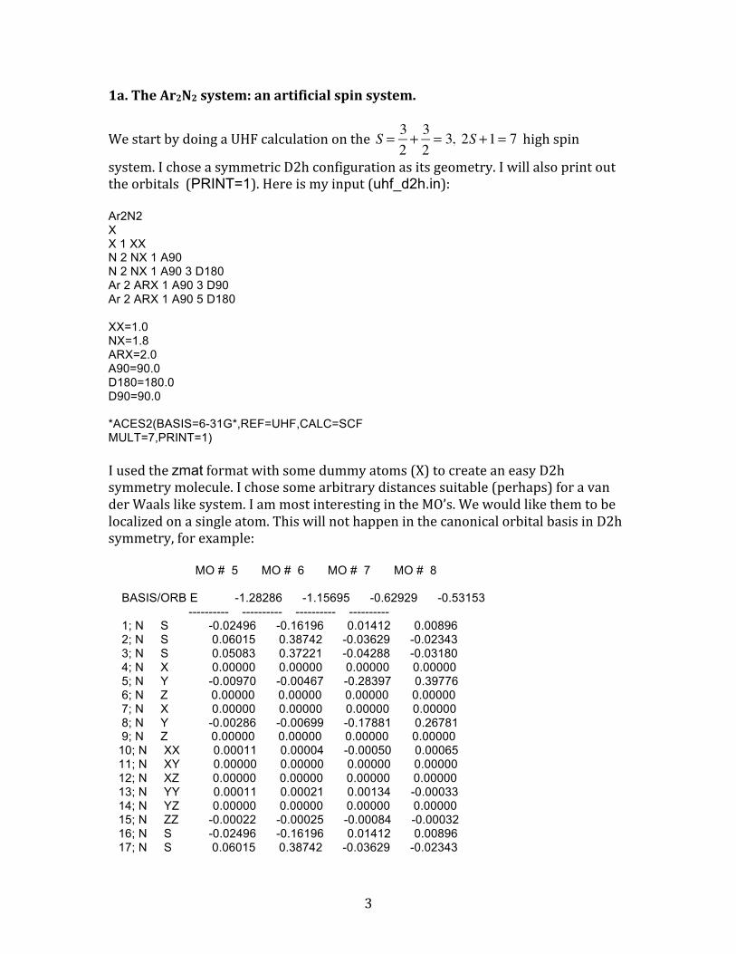
1a.  The  Ar2N2  system:  an  artificial  spin  system.    

We  start  by  doing  a  UHF  calculation  on  the   S = 32+ 32= 3, 2S +1= 7  high  spin  

system.  I  chose  a  symmetric  D2h  configuration  as  its  geometry.  I  will  also  print  out  the  orbitals    (PRINT=1).  Here  is  my  input  (uhf_d2h.in):    Ar2N2 X X 1 XX N 2 NX 1 A90 N 2 NX 1 A90 3 D180 Ar 2 ARX 1 A90 3 D90 Ar 2 ARX 1 A90 5 D180 XX=1.0 NX=1.8 ARX=2.0 A90=90.0 D180=180.0 D90=90.0 *ACES2(BASIS=6-31G*,REF=UHF,CALC=SCF MULT=7,PRINT=1)  I  used  the  zmat  format  with  some  dummy  atoms  (X)  to  create  an  easy  D2h  symmetry  molecule.  I  chose  some  arbitrary  distances  suitable  (perhaps)  for  a  van  der  Waals  like  system.  I  am  most  interesting  in  the  MO’s.  We  would  like  them  to  be  localized  on  a  single  atom.  This  will  not  happen  in  the  canonical  orbital  basis  in  D2h  symmetry,  for  example:     MO # 5 MO # 6 MO # 7 MO # 8 BASIS/ORB E -1.28286 -1.15695 -0.62929 -0.53153 ---------- ---------- ---------- ---------- 1; N S -0.02496 -0.16196 0.01412 0.00896 2; N S 0.06015 0.38742 -0.03629 -0.02343 3; N S 0.05083 0.37221 -0.04288 -0.03180 4; N X 0.00000 0.00000 0.00000 0.00000 5; N Y -0.00970 -0.00467 -0.28397 0.39776 6; N Z 0.00000 0.00000 0.00000 0.00000 7; N X 0.00000 0.00000 0.00000 0.00000 8; N Y -0.00286 -0.00699 -0.17881 0.26781 9; N Z 0.00000 0.00000 0.00000 0.00000 10; N XX 0.00011 0.00004 -0.00050 0.00065 11; N XY 0.00000 0.00000 0.00000 0.00000 12; N XZ 0.00000 0.00000 0.00000 0.00000 13; N YY 0.00011 0.00021 0.00134 -0.00033 14; N YZ 0.00000 0.00000 0.00000 0.00000 15; N ZZ -0.00022 -0.00025 -0.00084 -0.00032 16; N S -0.02496 -0.16196 0.01412 0.00896 17; N S 0.06015 0.38742 -0.03629 -0.02343

  4  

18; N S 0.05083 0.37221 -0.04288 -0.03180 19; N X 0.00000 0.00000 0.00000 0.00000 20; N Y 0.00970 0.00467 0.28397 -0.39776 21; N Z 0.00000 0.00000 0.00000 0.00000 22; N X 0.00000 0.00000 0.00000 0.00000 23; N Y 0.00286 0.00699 0.17881 -0.26781 24; N Z 0.00000 0.00000 0.00000 0.00000 25; N XX 0.00011 0.00004 -0.00050 0.00065 26; N XY 0.00000 0.00000 0.00000 0.00000 27; N XZ 0.00000 0.00000 0.00000 0.00000 28; N YY 0.00011 0.00021 0.00134 -0.00033 29; N YZ 0.00000 0.00000 0.00000 0.00000 30; N ZZ -0.00022 -0.00025 -0.00084 -0.00032  Because  of  the  3  planes  of  symmetry  all  orbitals  are  either  symmetric  or  antisymmetric  in  the  x,  y  or  z  plane.  I  would  like  the  open-­‐shell  orbitals  (the  p  orbitals  on  the  N-­‐atoms)  to  be  able  to  localize  (maintaining  some  symmetry  for  efficiency  reasons).  To  this  end  let  us  first  inspect  how  the  molecule  is  oriented  in  ACES2:     ----------------------------------------------- Cartesian coordinates corresponding to internal coordinate input (Angstroms) ---------------------------------------------------------------- Z-matrix Atomic C o o r d i n a t e s Symbol Number X Y Z ---------------------------------------------------------------- X 0 0.00000000 0.00000000 -1.00000000 X 0 0.00000000 0.00000000 0.00000000 N 7 0.00000000 1.80000000 0.00000000 N 7 -0.00000000 -1.80000000 0.00000000 AR 18 -2.00000000 0.00000000 0.00000000 AR 18 2.00000000 -0.00000000 0.00000000 ---------------------------------------------------------------- Interatomic distance matrix (Angstroms)  If  I  now  use  the  C2v  symmetry  group,  and  choose  the  y-­‐axis  as  the  C2  axis,  I  have  removed  the  symmetry  operation  interchanging  the  Nitrogen  atoms.  This  means  one  can  localize  orbitals  on  the  N-­‐atoms  while  maintaining  the  C2v  symmetry.  It  can  be  done  as  follows:    *ACES2(BASIS=6-31G*,REF=UHF,CALC=SCF MULT=7,SUBGROUP=C2V,PRINT=1 SUBGRPAXIS=Y)  I  use  a  C2v  group  oriented  such  that  the  planes  of  symmetry  are  the  horizontal  plane  of  the  molecule  and  the  plane  having  the  N-­‐N  axis.  In  practice  setting  things  up  this  may  involve  a  little  bit  of  twiddling  with  keywords  to  get  it  right  (that  is  what  I  did).  We  have  reached  our  goal  and  now  we  get  a  set  of  orbitals  that  are  grouped  (by  symmetry)  as  follows,  for  example,  (uhf.out0,  inspect  symmetry  block  1).    

  5  

MO # 9 MO # 10 MO # 11 MO # 12 BASIS/ORB E -1.15695 -0.62929 -0.60662 -0.54563 ---------- ---------- ---------- ---------- 1; N S -0.16196 0.01412 0.01306 0.00769 2; N S 0.38742 -0.03629 -0.03299 -0.02266 3; N S 0.37221 -0.04288 -0.04188 -0.02228 4; N X 0.00000 0.00000 0.00000 0.00000 5; N Y 0.00000 0.00000 0.00000 0.00000 6; N Z -0.00467 -0.28397 -0.24722 0.42838 7; N X 0.00000 0.00000 0.00000 0.00000 8; N Y 0.00000 0.00000 0.00000 0.00000 9; N Z -0.00699 -0.17881 -0.15282 0.28090 10; N XX -0.00025 -0.00084 -0.00072 -0.00040 11; N XY 0.00000 0.00000 0.00000 0.00000 12; N XZ 0.00000 0.00000 0.00000 0.00000 13; N YY 0.00004 -0.00050 0.00083 0.00099 14; N YZ 0.00000 0.00000 0.00000 0.00000 15; N ZZ 0.00021 0.00134 -0.00011 -0.00059 16; N S -0.16196 0.01412 -0.01306 -0.00769 17; N S 0.38742 -0.03629 0.03299 0.02266 18; N S 0.37221 -0.04288 0.04188 0.02228 19; N X 0.00000 0.00000 0.00000 0.00000 20; N Y 0.00000 0.00000 0.00000 0.00000 21; N Z 0.00467 0.28397 -0.24722 0.42838 22; N X 0.00000 0.00000 0.00000 0.00000 23; N Y 0.00000 0.00000 0.00000 0.00000 24; N Z 0.00699 0.17881 -0.15282 0.28090 25; N XX -0.00025 -0.00084 0.00072 0.00040 26; N XY 0.00000 0.00000 0.00000 0.00000 27; N XZ 0.00000 0.00000 0.00000 0.00000 28; N YY 0.00004 -0.00050 -0.00083 -0.00099 29; N YZ 0.00000 0.00000 0.00000 0.00000 30; N ZZ 0.00021 0.00134 0.00011 0.00059 You  can  see  that  both  the  symmetric  and  asymmetric  combinations  of  the  N  pz  like  orbital  reside  in  the  same  symmetry  block.  It  is  the  same  for  all  the  other  N  p-­‐orbitals.  That  is  what  we  want.  Now  we  can  localize  the  active  orbitals  using  a  special  procedure,  while  still  maintaining  C2v  symmetry.  We  set  up  the  CASSCF  calculation  in  the  usual  way  (use  probe_ci  etc.  to  figure  out  the  keywords).  I  will  first  optimize  the  high  spin  state.    *ACES2(BASIS=6-31G*,REF=UHF,CALC=CCSD MULT=7,SUBGROUP=C2V,SUBGRPAXIS=Y UNO_REF=ON,UNO_MULT=1,UNO_CHARGE=0 MAKERHF=ON,BRUECKNER=ON IP_CALC=IP_EOMCC,IP_SYM=2-2-2-0) *mrcc_gen closed_shell_calc=cas_ic_mrcc mcscf_calc=gtci *mcscf_info bruk_conv=7 magnetic_casmos=on

  6  

*gtci nele=6 nsymtype=1 multiplicity=1 7 state_irrep=1 1 states_per_symtype=1 1 *end  The  extra  keyword  is  given  by  magnetic_casmos=on.  The  program  carries  out  a  conventional  CASSCF  calculation  but  at  the  end  it  will  attempt  to  localize  the  orbitals  in  the  active  space.  If  you  search  in  the  output  file  for  @magnetic  you  will  see: Entered Magnetic Orbital module ********************************* Fmat @magnetic column 1 column 2 column 3 column 4 row 1 1003.42559421602 0.27597916635 0.00000000000 0.00000000000 row 2 0.27597916635 1003.43335995078 0.00000000000 0.00000000000 row 3 0.00000000000 0.00000000000 2007.42241302681 0.27909416847 row 4 0.00000000000 0.00000000000 0.27909416847 2007.42390876978 row 5 0.00000000000 0.00000000000 0.00000000000 0.00000000000 row 6 0.00000000000 0.00000000000 0.00000000000 0.00000000000 column 5 column 6 row 1 0.00000000000 0.00000000000 row 2 0.00000000000 0.00000000000 row 3 0.00000000000 0.00000000000 row 4 0.00000000000 0.00000000000 row 5 3011.42538124633 0.28099108540 row 6 0.28099108540 3011.42524077475  The  program  will  diagonalize  this  “Fmat”,  yielding  Cmat0,  and  in  the  end  it  tries  to  localize  the  exchange  integrals  using  the  new  orbitals.  This  yields  Kmat  in  the  output  file.  The  procedure  is  iterative,  but  here,  for  the  Ar2N2  system,  we  get  a  nice  set  of  localized  K  exchange  integrals   ab ba  in  one  shot:     transformed integrals @magnetic Kmat column 1 column 2 column 3 column 4 row 1 0.70530607453 0.00009555093 0.03563169000 0.00000203247 row 2 0.00009555093 0.70541532312 0.00000677947 0.03563658507 row 3 0.03563169000 0.00000677947 0.70224983475 0.00000322800 row 4 0.00000203247 0.03563658507 0.00000322800 0.70225384278 row 5 0.00000748505 0.03549170690 0.00000062403 0.03564453689 row 6 0.03548653465 0.00001263897 0.03564435066 0.00000080480

  7  

column 5 column 6 row 1 0.00000748505 0.03548653465 row 2 0.03549170690 0.00001263897 row 3 0.00000062403 0.03564435066 row 4 0.03564453689 0.00000080480 row 5 0.70629334357 0.00000873482 row 6 0.00000873482 0.70629337868    This  is  a  6x6  matrix  (nact  x  nact)  and  the  orbitals  are  rotated  [maintaining  C2v  symmetry,  yielding  3  pairs  of  orbitals  (recall:  IP_SYM=2-­‐2-­‐2-­‐0)  ],  and  minimizing  the  off-­‐diagonal  elements  of  the  K-­‐matrix.    This  K-­‐matrix  at  the  end  of  the  calculation  is  the  important  quantity.  We  would  preferably  have  large  elements  on  the  diagonal  only.  The  remaining  (somewhat)  larger  elements  (0.035  ..)  involve  orbitals  of  different  symmetries,  which  are  not  allowed  to  mix.  The  file  mcscf_mos  will  contain  these  localized  orbitals  if  we  include  the  magnetic_casmos  keyword.    These  localized  orbitals  are  extremely  useful  as  all  low  lying  electronic  states  can  be  characterized  by  having  one  electron  in  each  spatial  orbital  (of  either  alpha  or  beta  spin).  For  this  system  we  have  6  electrons  in  6  spatial  orbitals.      Now  we  can  do  probe_CI  calculations  to  pick  up  the  low  lying  states  of  all  multiplicities  (7,5,3,1  here)  and  set  up  the  final  mcscf calculation  that  optimizes  the  orbitals  for  the  average  ensemble.  Here  is  the  relevant  section  of  the  input  file:      *mrcc_gen closed_shell_calc=cas_ic_mrcc mcscf_calc=gtci *mcscf_info bruk_conv=7 read_mos=on magnetic_casmos=on *gtci select_magnetic=on nele=6 nsymtype=4 multiplicity=4 7 5 3 1 state_irrep=4 1 1 1 1 states_per_symtype=4 1 1 1 1 *end    As  before  we  have  the  keyword  magnetic_casmos=on,  which  tells  the  program  to  maintain  localized  orbitals.  In  addition  I  included  the  additional  keyword  select_magnetic=on.  This  keyword  tells  the  program  we  are  interested  in  those  states  in  which  we  have  as  many  singly  occupied  orbitals  as  possible  (here  6,  as  we  we  have  6  electrons  and  6  orbitals).  This  “magnetic  subset”  is  in  general  a  small  susbset  of  all  possible  determinants  in  the  CAS,  and  it  will  allow  us  to  get  good  

  8  

guesses  for  the  states,  even  when  the  CAS  is  getting  very  large.    The  program  prints  a  bit  of  a  cryptic  message  to  compare  these  two  dimensions,  e.g.      

smci_dim : 6 dim_active 12  (smci_dim  is  the  dimension  of  the  small  CI  (=magnetic  CI)  diagonalization).  The  difference  between  these  two  spaces  can  get  more  impressive  as  we  increase  the  number  of  active  orbitals.  We’ll  see  examples  later  on.      During  the  CAS  iteration  stage  you  will  now  get  two  sets  of  summaries:   ********************************************************************************** * Summary of Magnetic CI calculation * ********************************************************************************** Serial 2S+1 2*Sz irrep iroot E_Excite/eV E_Excite/cm-1 E-total ********************************************************************************** 1 7 6 [1] 1 0.0000 0.00 -1162.2759546592 2 5 4 [1] 1 0.0024 19.70 -1162.2758649006 3 3 2 [1] 1 0.0041 32.85 -1162.2758049947 4 1 0 [1] 1 0.0049 39.43 -1162.2757750216 **********************************************************************************  and    ****************************************************************************************************** * Summary of CASSCF/CASCI calculation * ****************************************************************************************************** Serial 2S+1 2*Sz irrep iroot E_Excite/eV E_Excite/cm-1 Residual Overlap Select E-total ****************************************************************************************************** 1 7 6 [1] 1 0.0000 0.00 0.00E+00 1.000 T -1162.2759546592 2 5 4 [1] 1 0.0007 5.36 0.20E-05 1.000 T -1162.2759302161 3 3 2 [1] 1 0.0011 8.94 0.57E-05 1.000 T -1162.2759139184 4 1 0 [1] 1 0.0013 10.73 0.85E-05 1.000 T -1162.2759057688 ******************************************************************************************************  The  “magnetic  CI”  calculation  only  includes  the  “magnetic”  determinants.  This  space  is  CAS-­‐complete  for  the  7-­‐tet  (1  determinant  only),    but  is  not  complete  for  the  lower  spin  states  (you  can  inspect  the  dimension  of  the  CAS).    You  can  observe  that  the  energy  for  the  7-­‐tet  is  identical  in  the  two  calculations.  Another  thing  that  may  strike  you  is  that  the  energy  differences  between  the  various  spin  states  are  very  small  indeed  (order  of  cm-­‐1).    Moreover,  the  excitation  energies  are  smaller  in  the  CASCI  than  in  the  magnetic  CI  calculation.  This  makes  perfect  sense.  The  ground  state  7-­‐tet  has  the  same  energy  in  both  calculations,  while  the  other  states  in  the  CASCI  calculation  are  lower  in  energy  than  in  the  magnetic  CI,  because  the  diagonalization  space  is  larger    in  the  CAS  (variational  principle  at  work).  Still  the  energy  lowering  is  very  minor  (~15  cm-­‐1  )!,  indicating  that  the  magnetic  CI  is  qualitatively  correct.  

  9  

Calculations  on  so-­‐called  magnetic  systems  are  all  about  getting  these  minute  energy  splittings  correct,  so  there  is  a  significant  change  due  to  the  use  of  the  full  CAS.    Let  me  examine  one  more  interesting  part  of  the  output:  The  section  that  prints  out  the  character  of  the  eigenstates.  I  will  look  at  the  singlet  states  in  symmetry  block  1.  This  is  what  we  get:   ************************************************* Canonically Orthogonalized Active Target States ************************************************* spin quantum number S ..... = 0.000 spin eigenvalue S*(S+1) ..... = 0.000 spin multiplicity 2S+1 ..... = 1 spin Z-component 2*Sz ..... = 0 spatial symmetry irrep ..... = 1 number of states targeted ..... = 1 Dimension of active space ..... = 112 ************************************************* State Energy ! S(S+1)!Trace-DM1!Trace-DM2 ************************************************* 1 -6.211479751 0.000 okay okay ************************************************* Active Orbital Energies ------------------------ Irrep: 1 1.864326 1.864638 Irrep: 2 1.864326 1.864638 Irrep: 3 1.864326 1.864638 Irrep: 4 ------------------------ **************************************************************************************************** determinant coefficients occupation-pattern **************************************************************************************************** State # 1 [11|22|33|11|22|33] 53 -0.500 [A-|A-|-A|-B|-B|B-] 60 -0.500 [-A|-A|A-|B-|B-|-B] ****************************************************************************************************  The  total  dimension  of  the  CAS,  while  you  can  verify  that  the  dimension  of  the  magnetic  CI  calculation  is  only  20.  Most  interesting  is  the  pattern  of  the  determinants.  You  can  see  that  each  orbital  is  occupied  by  either  an  alpha  or  a  beta  electron,  but  never  by  both.  The  final  CASCI  wave  funtions  are  quite  compact.  The  next  step  is  inclusion  of  dynamical  correlation  effects  using  the  mreom_try  setup.  Here  is  the  gtci part  of  the  input:    

  10  

*gtci_final include_hh=off include_1h=on include_1p=on include_phh=off include_ph=off select_magnetic=on nele=6 nsymtype=4 multiplicity=4 7 5 3 1 state_irrep=4 1 1 1 1 states_per_symtype=4 1 1 1 1 *gtci select_magnetic=on nele=6 nsymtype=4 multiplicity=4 7 5 3 1 state_irrep=4 1 1 1 1 states_per_symtype=4 1 1 1 1 *end You  can  see  I  put  in  select_magnetic  in  both  of  the  gtci  sections.  The  final  result  of  the  calculation,  including  dynamical  correlation  from  the  mreom_try.in  calculation  is  posted  below:    ****************************************************************************************************** * Summary of pIC-MRCC/MR-EOMCC calculation * ****************************************************************************************************** Serial 2S+1 2*Sz irrep iroot E_Excite/eV E_Excite/cm-1 Residual Overlap %Active E-total ****************************************************************************************************** 1 7 6 [1] 1 0.0000 0.00 0.22E-07 1.000 99.9% -1162.7559015127 2 5 4 [1] 1 0.0006 4.88 0.85E-07 1.000 99.9% -1162.7558792593 3 3 2 [1] 1 0.0010 8.14 0.71E-07 1.000 99.9% -1162.7558644239 4 1 0 [1] 1 0.0012 9.77 0.75E-07 1.000 99.9% -1162.7558569951 ******************************************************************************************************  You  can  see  that  the  excitation  energies  do  not  change  all  that  much  due  to  inclusion  of  dynamical  correlation  (compare  to  CASSCF  results).  That  is  of  course  not  always  the  case.  This  concludes  the  treatment  of  the  Ar2N2  system.    1b.  The  Ar2O2  system:  a  second  artificial  spin  system.    The  second  spin  system  we  will  investigate  is  similar.  I  just  replaced  N  by  O.  To  get  a  set  of  orbitals  that  treat  the  p-­‐orbitals  on  oxygen  in  an  equivalent  way  I  started  from  

  11  

a  UHF  calculation  of  the  2+  system,  a  septet  as  for  the  previous  system  Ar2N2.  The  issue  with  localizing  the  orbitals  works  the  same  as  before.  I  run  the  calculations  using  C2v  symmetry,  and  orient  the  C2  axis  along  y.  Next  I  run  a  probe_CI  calculation  to  figure  out  what  the  symmetries  of  the  lowest  energy  states  are.  I  can  couple  the  two  triplets  of  O-­‐atoms  into  an  S=1+1=2,  or  quintet  multiplicity.  I  ended  running  my  initial  MCSCF  calculation  (for  9  different  quintet  states)  using  the  following  input:    Ar2O2 X X 1 XX O 2 OX 1 A90 O 2 OX 1 A90 3 D180 Ar 2 ARX 1 A90 3 D90 Ar 2 ARX 1 A90 5 D180 XX=1.0 OX=1.8 ARX=2.0 A90=90.0 D180=180.0 D90=90.0 *ACES2(BASIS=6-31G*,REF=UHF,CALC=CCSD CHARGE=2 DROPMO=1>12,MULT=7,SUBGROUP=C2V,SUBGRPAXIS=Y UNO_REF=ON,UNO_MULT=1,UNO_CHARGE=0 MAKERHF=ON,BRUECKNER=ON IP_CALC=IP_EOMCC,IP_SYM=2-2-2-0) *mrcc_gen closed_shell_calc=cas_ic_mrcc mcscf_calc=gtci *mcscf_info bruk_conv=7 magnetic_casmos=on *gtci select_magnetic=on nele=8 nsymtype=4 multiplicity=4 5 5 5 5 state_irrep=4 1 2 3 4 states_per_symtype=4 3 2 2 2  The  additional  keywords  to  perform  the  orbital  localization  at  the  end  (magnetic_casmos)  ,  and  the  use  of  select_magnetic  keyword  to  select  states  is  used  as  before.  In  total  we  have  9  quintet  multiplets  (or  45  electronic  states).  You  can  also  find  the  triplet  and  singlet  states,  and  count  that  in  total  we  have  9  x  9  =  81  states  in  a  fairly  small  energy  window.    You  should  have  acquired  all  the  knowledge  now  to  push  the  calculation  to  completion.  Let  me  list  my  final  results  for  your  perusal:  

  12  

****************************************************************************************************** * Summary of pIC-MRCC/MR-EOMCC calculation * ****************************************************************************************************** Serial 2S+1 2*Sz irrep iroot E_Excite/eV E_Excite/cm-1 Residual Overlap %Active E-total ****************************************************************************************************** 1 5 4 [1] 1 0.0000 0.00 0.58E-07 0.997 99.4% -1203.6153997602 2 3 2 [1] 1 0.0008 6.25 0.43E-07 0.997 99.4% -1203.6153712892 3 1 0 [1] 1 0.0012 9.37 0.94E-07 0.997 99.4% -1203.6153570477 4 5 4 [2] 1 0.0991 799.24 0.41E-07 0.997 99.4% -1203.6117581515 5 3 2 [2] 1 0.0992 799.79 0.57E-07 0.997 99.4% -1203.6117556451 6 1 0 [2] 1 0.0992 800.07 0.55E-07 0.997 99.4% -1203.6117543890 7 5 4 [2] 2 0.1060 855.24 0.77E-07 0.997 99.4% -1203.6115029849 8 3 2 [2] 2 0.1062 856.88 0.70E-07 0.997 99.4% -1203.6114955450 9 1 0 [2] 2 0.1063 857.69 0.53E-07 0.997 99.4% -1203.6114918203 10 5 4 [4] 1 0.1370 1104.60 0.96E-07 0.997 99.4% -1203.6103668228 11 3 2 [4] 1 0.1376 1109.64 0.80E-07 0.997 99.4% -1203.6103438493 12 1 0 [4] 1 0.1379 1112.17 0.84E-07 0.997 99.4% -1203.6103323560 13 5 4 [4] 2 0.1383 1115.53 0.66E-07 0.997 99.4% -1203.6103170370 14 3 2 [4] 2 0.1389 1120.13 0.66E-07 0.997 99.4% -1203.6102960619 15 1 0 [4] 2 0.1392 1122.44 0.50E-07 0.997 99.4% -1203.6102855694 16 1 0 [1] 2 0.2193 1768.71 0.85E-07 0.997 99.4% -1203.6073409153 17 3 2 [1] 2 0.2193 1768.82 0.97E-07 0.997 99.4% -1203.6073404060 18 5 4 [1] 2 0.2193 1769.04 0.55E-07 0.997 99.4% -1203.6073394020 19 5 4 [3] 1 0.2369 1910.81 0.95E-07 0.997 99.4% -1203.6066934634 20 3 2 [3] 1 0.2371 1912.51 0.60E-07 0.997 99.4% -1203.6066857305 21 1 0 [3] 1 0.2372 1913.36 0.46E-07 0.997 99.4% -1203.6066818636 22 5 4 [3] 2 0.2491 2009.15 0.21E-07 0.997 99.4% -1203.6062454120 23 3 2 [3] 2 0.2492 2009.80 0.47E-07 0.997 99.4% -1203.6062424343 24 1 0 [3] 2 0.2492 2010.13 0.41E-07 0.997 99.4% -1203.6062409442 25 5 4 [1] 3 0.2851 2299.15 0.47E-07 0.997 99.4% -1203.6049240537 26 3 2 [1] 3 0.2855 2302.85 0.46E-07 0.997 99.4% -1203.6049072134 27 1 0 [1] 3 0.2857 2304.70 0.81E-07 0.997 99.4% -1203.6048987848 ******************************************************************************************************  You  can  see  that  the  %active  behaves  beautifully  in  these  magnetic  systems.  I  imagine  the  results  to  be  quite  accurate.    Excercises  on  magnetic  systems:    

1. Remove  one  electron  from  the  Ar2N2  system  (setting  nele).  This  would  describe  a  1  hole  state  within  the  spin  manifold.  We  are  making  our  way  to  spintronics!  You  can  calculate  the  energy  levels  for  such  a  system.  You  can  use  the  orbitals  mcscf_mos  of  the  neutral  as  a  first  guess.  

2. Add  one  electron  to  the  Ar2O2  system  (again  by  adjusting  nele).  Use  the  mcscf_mos  of  the  neutral  as  a  first  guess.  

3. Consider  the  Mn2O2  system  (  a  long  problem,  optional).  Use  the  D2h  geometry  setup  as  for  the  other  systems  using  an  MnX  distance  of    1.30  Å,  and  an  OX  distance  of  1.4  Å  (that  was  my  guess).    I  took  the  high  spin  system  to  have  

S = 52+ 52,(2S +1) = 11 ,  and  I  used  an  Ahlrichs-VDZ  basis  set.  The  magnetic  

  13  

system  now  resides  on  the  metal  centers  of  course.  Now  we  have  10  open  shell  orbitals  and  the  dimension  of  the  CAS  grows  rapidly.  Using  the  select_magnetic  keyword  is  crucial  to  get  results.  I  have  not  yet  fully  completed  the  calculation,  and  the  low-­‐spin  states  might  become  too  demanding.  You  will  have  to  monitor  and  see  how  far  you  can  push  the  calculations  (i.e.  regarding  including  low  spin  states  in  the  calculation).      2.  Calculations  on  the  Fe  atom:  Use  of  a  weighted  average  CASSCF  calculation.    For  neutral  transition  metal  atoms  we  typically  get  electronic  states  of  two  different  character:  states  with  one  electron  in  the  4s  orbital,  for  the  Fe  atom  this  would  be  states  of  4s13d7  character  (8  active  electrons  in  total),  and  states  that  have    4s23d6  character.  Let  us  look  at  a  little  piece  of  the  “NIST  atomic  energy  levels”  data  for  the  Fe  atom:    

Configuration Term J Level (eV)

Landé-g Leading percentages Reference

3d64s2 a 5D 4 0.000000 1.50020 100

L11631

3 0.0515691 1.50034 100

2 0.0872857 1.50041 100

1 0.110114 1.50022 100

0 0.121266 100

3d7(4F)4s a 5F 5 0.8589957 1.40021 100

4 0.9146021 1.35004 100

3 0.9581573 1.24988 100

  14  

2 0.9901111 0.99953 100

1 1.011056 -0.014 100

3d7(4F)4s a 3F 4 1.4848643 1.254 98

1 3d64s2 3F2

3 1.5573572 1.086 98

1 3d64s2 3F2

2 1.6078957 0.670 98

1 3d64s2 3F2

3d7(4P)4s a 5P 3 2.1759450 1.666 99

2 2.1978663 1.820 99

1 2.2227120 2.499 99

   

Let  us  set  as  our  goal  to  create  a  weighted  CASSCF  ensemble  that  has  the  two  lowest  multiplets  in  Fe,  the  5D(4s2)  and  5F(4s1)  states,  weighted  such  that  the  average  occupation  of  the  4s  orbital  is  1.5  approximately.  In  my  group  we  have  found  that  using  such  an  average  occupation  works  quite  well  for  the  complete  excitation  spectrum  (an  empirical  observation).  I  first  run  a  UHF  calculation  on  the  totally  spherically  symmetric  4s13d5  state,  which  has  only  6  active  electrons.  This  means  the  Fe  atom  will  have  charge  +2.    From  the  UHF  calculation  I  learn  the  symmetries  of  the  active  orbitals,  and  I  can  set  up  the  uhf_probe_CI  calculation  for  the  quintet  states  (setting  nele=8  to  get  the  neutral).  Below  are  the  input  and  output  files.  I  am  using  the  Def2-­‐TZVPPD  basis  set  again,  which  seems  to  work  very  well.    There  is  a  special  feature,  as  we  wish  to  include  scalar  relativistic  effects.  This  can  be  done  by  including  the  keyword  DKH_ORDER=-1.  This  is  the  simplest  way  to  account  for  some  relativistic  effects.    

  15  

Input  file  uhf_probe_5.in:    Fe atom cas Fe *ACES2(BASIS=Def2-TZVPPD,CHARGE=2,REF=UHF,CALC=CCSD MULT=7,DKH_ORDER=-1 SUBGROUP=D2 UNO_REF=ON,UNO_MULT=1,UNO_CHARGE=0 MAKERHF=ON BRUECKNER=ON IP_CALC=IP_EOMCC,IP_SYM=3-1-1-1 DIP_CALC=EOMCC,DIP_SYM=1-0-0-0) *mrcc_gen closed_shell_calc=ccsd mcscf_calc=gtci *mcscf_info bruk_conv=7 read_mos=off probeci=on *gtci nele=8 probe_states=10 probe_multi=5 probe_irrep=0 *end  Summary  part  of  the  output  file:    *********************************************************************************************************** * Summary of MCSCF probe-CI: energy of states by irrep * *********************************************************************************************************** state irrep irrep irrep irrep 1 2 3 4 *********************************************************************************************************** 1 -8.6743770 -8.6743770 -8.6743770 -8.6743770 2 -8.6743770 -8.1871787 -8.1871787 -8.1871787 3 -8.1871787 -8.1871787 -8.1871787 -8.1871787 4 unavailable -8.0984199 -8.0984199 -8.0984199 5 unavailable unavailable unavailable unavailable 6 unavailable unavailable unavailable unavailable  Since  the  orbitals  for  the  di-­‐cation  can  be  expected  to  be  quite  poor  I  do  a  first  mcscf_a.in  calculation  in  which  I  will  optimize  the  average  of  the  5D  and  5F  states.  You  can  verify  that  the  following  gtci  sector  input  is  appropriate:  

  16  

 *mcscf_info read_mos=off bruk_conv=7 *gtci nele=8 nsymtype=4 multiplicity=4 5 5 5 5 state_irrep=4 1 2 3 4 states_per_symtype=4 3 3 3 3 *end You  can  verify  furthermore  that  the  degeneracy  of  the  states  is  nicely  maintained  in  the  calculation  (monitor  the  various  instances  of  the  Summary of CASSCF/CASCI).    At  the  end  of  the  mcscf_a  calculation  I  got:    ****************************************************************************************************** * Summary of CASSCF/CASCI calculation * ****************************************************************************************************** Serial 2S+1 2*Sz irrep iroot E_Excite/eV E_Excite/cm-1 Residual Overlap Select E-total ****************************************************************************************************** 1 5 4 [3] 1 0.0000 0.00 0.12E-14 1.000 T -1270.7328262673 2 5 4 [2] 1 0.0000 0.00 0.17E-14 1.000 T -1270.7328262673 3 5 4 [4] 1 0.0000 0.00 0.20E-15 1.000 T -1270.7328262673 4 5 4 [1] 1 0.0000 0.00 0.22E-21 1.000 T -1270.7328262664 5 5 4 [1] 2 0.0000 0.00 0.16E-14 1.000 T -1270.7328262664 6 5 4 [1] 3 1.3637 10998.63 0.20E-21 1.000 T -1270.6827128398 7 5 4 [3] 2 1.3637 10998.63 0.89E-15 1.000 T -1270.6827128382 8 5 4 [4] 2 1.3637 10998.63 0.28E-14 1.000 T -1270.6827128382 9 5 4 [2] 2 1.3637 10998.63 0.27E-14 1.000 T -1270.6827128382 10 5 4 [4] 3 1.3637 10998.63 0.89E-15 1.000 T -1270.6827128369 11 5 4 [2] 3 1.3637 10998.63 0.89E-15 1.000 T -1270.6827128369 12 5 4 [3] 3 1.3637 10998.63 0.89E-15 1.000 T -1270.6827128369 ******************************************************************************************************  It  is  also  of  interest  to  inspect  the  character  of  the  states.  If  I  look  in  the  last  symmetry  block  (4),  I  see  we  should  get  one  component  of  the  D  multiplet  (structure  by  symmetry  2-­‐1-­‐1-­‐1,  see  later  also),  and  2  components  of  the  F-­‐multiplet  (structure  by  symmetry  1-­‐2-­‐2-­‐2)  .  From  the  NIST  table  we  anticipate  the  5D  state  to  have  4s2  character,  while  the  5F  states  ought  to  have  4s1  character.    Can  we  get  this  from  the  output  file?    Let  us  look  at  the  section  where  it  prints  the  characters  of  the  states  (symmetry  block  4,  the  last  symmetry  block):    

  17  

************************************************* Canonically Orthogonalized Active Target States ************************************************* spin quantum number S ..... = 2.000 spin eigenvalue S*(S+1) ..... = 6.000 spin multiplicity 2S+1 ..... = 5 spin Z-component 2*Sz ..... = 4 spatial symmetry irrep ..... = 4 number of states targeted ..... = 3 Dimension of active space ..... = 4 ************************************************* State Energy ! S(S+1)!Trace-DM1!Trace-DM2 ************************************************* 1 -5.277600381 6.000 okay okay 2 -5.227486951 6.000 okay okay 3 -5.227486950 6.000 okay okay ************************************************* Active Orbital Energies ------------------------ Irrep: 1 -0.180666 -0.180666 -0.156097 Irrep: 2 -0.180666 Irrep: 3 -0.180666 Irrep: 4 -0.180666 ------------------------ **************************************************************************************************** determinant coefficients occupation-pattern **************************************************************************************************** State # 1 [111|2|3|4|111|2|3|4] 4 1.000 [AAA|A|A|A|--B|-|-|B] **************************************************************************************************** State # 2 [111|2|3|4|111|2|3|4] 2 0.847 [AAA|A|A|A|B--|-|-|B] 3 -0.531 [AAA|A|A|A|-B-|-|-|B] **************************************************************************************************** State # 3 [111|2|3|4|111|2|3|4] 1 0.894 [AAA|A|A|A|---|B|B|-] 2 -0.237 [AAA|A|A|A|B--|-|-|B] 3 -0.379 [AAA|A|A|A|-B-|-|-|B] ****************************************************************************************************  

  18  

A  lot  of  info  here.  Let  us  digest.  I  used  bold  face  to  indicate  we  are  looking  at  symmetry  block  4.  The  relative  energies  of  the  states  are  also  highlighted.  You  can  see  the  second  and  third  state  are  degenerate  (F  here),  while  the  lowest  state  is  the  component  of  the  D  state.  Next  the  program  prints  Active Orbital Energies.  You  see  5  degenerate  orbital  energies,  corresponding  to  the  3d  orbitals,  and  1  higher  lying  energy,  which  must  be  the  4s  orbital.  The  orbitals  are  ordered  in  this  fasion  in  the   [111|2|3|4|111|2|3|4] string,  which  only  indicates  the  spatial  symmetry  of  the  orbitals  for  the  alpha  and  beta  spin  orbitals.  The  3rd  orbital  in  block  1  refers  to  the  4s  orbital,  all  the  other  orbitals  have  d  character.  (You  get  this  information  by  looking  at  the  Active Orbital Energies).  The  alpha  electrons  are  completely  filled,  while  the  occupation  of  the  beta  spin  orbitals  varies.    You  can  see  that  the  3rd  orbital  (beta  spin)  of  symmetry  [1]  is  populated  in  the  lowest  energy  state.  This  means  this  state  has  overall  2  electrons  in  the  4s  orbital.  We  would  characterize  it  as  a  4s23d6  configuration,  and  we  know  it  is  spatially  5-­‐fold  degenerate,  with  spin  multiplicity  5,  or  a  5D  multiplet,  representing  25  electronic  states  in  total(!).    You  can  also  see  that  the  second  and  third  state  in  block  4  do  not  have  a  beta  electron  in  the  3rd  orbital  of  symmetry  [1],  and  hence  they  correspond  to  the  4s13d7  configuration,  and  we  know  it  is  spatially  7-­‐fold  degenerate,  with  spin  multiplicity  5,  or  a  5F  multiplet,  representing  35  electronic  states  in  total.  So  you  can  see  we  can  in  principle  get  all  of  this  information  from  the  calculations,  without  having  to  confirm  with  the  NIST  experimental  data.  It  is  nice,  of  course,  to  see  the  NIST  data  agrees  in  regards  to  the  ordering  of  the  levels.  This  is  not  necessarily  the  case  at  this  initial  CASSCF  level  of  accuracy.  You  can  also  observe  there  is  substantial  splitting  of  the  experimental  data  within  one  L-­‐S  multiplet.  The  J-­‐values  for  5D  (L=2,  S=2)  run  from  J=4,…,0.  This  is  due  to  spin-­‐orbit  coupling  which  is  not  (yet)  included  in  these  calculations.  We  should  compare  to  the  experimental    J-­‐averaged  energies  therefore  when  evaluating  the  excitation  energies  from  the  electronic  structure  calculations.  You  can  observe  that  the  agreement  is  not  all  that  good,  but  keep  in  mind  we  have  done  only  a  state-­‐averaged  CASSCF  calculation  thus  far.    Let  us  analyse  one  further  piece  of  output  near  the  end  of  the  file:     Analysis of one-particle density matrix ------------------------------------------- natural occupation in irrep 1 column 1 row 1 1.41666666667 row 2 1.31666666765 row 3 1.31666666765 Natural orbitals in H0 basis column 1 column 2 column 3 row 1 -0.00000000000 0.98517456897 -0.17155485613 row 2 -0.00000000016 0.17155485613 0.98517456897 row 3 1.00000000000 0.00000000003 0.00000000016 natural occupation in irrep 2 column 1

  19  

row 1 1.31666666601 There  is  some  further  info  for  blocks  3  and  4  (not  listed  here).    Here  you  observe  the  average  occupations  of  the  4s  (1.41666)  and  the  degenerate  3d  (1.31666)  orbitals.    The  program  also  prints  out  the  so-­‐called  natural  orbitals,  but  this  provides  limited  information.  I  would  like  to  make  the  average  occupation  of  the  4s  orbital  1.5  (or  

close  to  it).    This  I  can  do  by  giving  the  5D  state  a  weight  of   712,  while  the  5F  state  

should  have  a  weight  of   512.  The  only  importance  is  the  ratio  of  the  weights,  which  I  

might  choose  as  0.07  and  0.05.  The  program  will  normalize  the  total  weight  to  1.    So  now  I  run  a  second  mcscf_b  calculation,  specifying  the  weight  for  each  state,  such  that  I  can  expect  the  overall  weight  of  the  4s  orbital  to  be  close  to  1.5.  Here  is  the  *gtci  section  (following  mcscf_weighted.in  in  MREOM_standard_inputs):    *mcscf_info read_mos=on bruk_conv=7 *gtci nele=8 nstates=12 multiplicity=12 5 5 5 5 5 5 5 5 5 5 5 5 state_irrep=12 1 1 1 2 2 2 3 3 3 4 4 4 state_weight=12 0.07 0.07 0.05 0.07 0.05 0.05 0.07 0.05 0.05 0.07 0.05 0.05 *end In  the  state_weight  section  the  program  assumes  the  energy  ordering  that  comes  out  of  the  CASSCF  calculation  (here  D  lowest,  then  F).  This  order  might  potentially  change  as  the  orbitals  are  optimized  (in  particular  if  there  is  only  a  small  gap  between  states).  This  does  not  happen  here.  If  it  does  one  would  have  to  piddle  around  to  get  the  orbitals  (very)  close  to  convergence  and  try  to  get  the  order  not  to  change  anymore.    At  intermediate  stages  of  the  process  or  your  sequence  of  calculations  the  orbitals  may  break  the  spherical  degeneracy  pattern.  (I  am  sure  the  programmer  could  facilitate  things  with  a  bit  of  work  to  track  states.  After  enough  complaints  I  might  implement  something).  Let  us  not  get  into  these  issues  here.    You  can  observe  that  the  program  is  somewhat  slow  to  converge  (grep –a “MCSCF total” mcscf_b.out0):   First Brueckner residual : 0.831E-02 iteration 1 MCSCF total energy : -1270.7077695824 Max Brueckner residual : 0.388E-02 iteration 2 MCSCF total energy : -1270.7084185348 Max Brueckner residual : 0.155E-02 iteration 3 MCSCF total energy : -1270.7085444604 Max Brueckner residual : 0.991E-03 iteration 4 MCSCF total energy : -1270.7085653884 Max Brueckner residual : 0.669E-03 iteration 5 MCSCF total energy : -1270.7085731175 Max Brueckner residual : 0.754E-03 iteration 6 MCSCF total energy : -1270.7085713690 Max Brueckner residual : 0.319E-03 iteration 7 MCSCF total energy : -1270.7085780316 Max Brueckner residual : 0.994E-03 iteration 8 MCSCF total energy : -1270.7085657431 Max Brueckner residual : 0.434E-03 iteration 9 MCSCF total energy : -1270.7085765305

  20  

Max Brueckner residual : 0.200E-03 iteration 10 MCSCF total energy : -1270.7085788005 Max Brueckner residual : 0.146E-03 iteration 11 MCSCF total energy : -1270.7085790955 Max Brueckner residual : 0.669E-04 iteration 12 MCSCF total energy : -1270.7085793547 Max Brueckner residual : 0.311E-04 iteration 13 MCSCF total energy : -1270.7085794107 Max Brueckner residual : 0.157E-04 iteration 14 MCSCF total energy : -1270.7085794222 Max Brueckner residual : 0.722E-05 iteration 15 MCSCF total energy : -1270.7085794253 Max Brueckner residual : 0.339E-05 iteration 16 MCSCF total energy : -1270.7085794259 Max Brueckner residual : 0.158E-05 iteration 17 MCSCF total energy : -1270.7085794261 Max Brueckner residual : 0.743E-06 iteration 18 MCSCF total energy : -1270.7085794261 Max Brueckner residual : 0.380E-06 iteration 19 MCSCF total energy : -1270.7085794261 Max Brueckner residual : 0.398E-06 iteration 20 MCSCF total energy : -1270.7085794261 Max Brueckner residual : 0.188E-06 iteration 21 MCSCF total energy : -1270.7085794261 Max Brueckner residual : 0.858E-07 iteration 22 MCSCF total energy : -1270.7085794261  But  at  the  end  of  the  course  if  we  now  inspect  the  natural  occupation  numbers  we  find:     Analysis of one-particle density matrix ------------------------------------------- natural occupation in irrep 1 column 1 row 1 1.50000000000 row 2 1.30000000069 row 3 1.30000000069 Natural orbitals in H0 basis column 1 column 2 column 3 row 1 -0.00000000001 0.89487805081 -0.44631073723 row 2 -0.00000000016 0.44631073723 0.89487805081 row 3 1.00000000000 0.00000000008 0.00000000014 natural occupation in irrep 2 column 1 row 1 1.29999999954 Natural orbitals in H0 basis  And  we  hence  observe  that  the  4s  orbital  is  indeed  populated  on  average  by  1.5  electrons,  as  was  desired.  Next  we  can  run  an  mreom_try.in  calculation  in  the  usual  fashion  to  make  sure  the  T-­‐amplitudes  are  all  well  behaving,  and  run  the  probe_*.in  calculations  to  select  the  states  we  want  to  include  in  the  final  calculation.    Let  me  post  the  summarizing  output  for  the  probe_1.out0  file:  

  21  

********************************************************************************************************** state irrep irrep irrep irrep 1 2 3 4 ********************************************************************************************************** 1 -5.2682429 -5.2682429 -5.2682429 -5.2682429 2 -5.2682429 -5.2682429 -5.2682429 -5.2682429 3 -5.2682429 -5.2682429 -5.2682429 -5.2682429 13 states -> I 4 -5.2682429 -5.2611244 -5.2611244 -5.2611244 5 -5.2611244 -5.2611244 -5.2611244 -5.2611244 9 states -> G 6 -5.2611244 -5.2397002 -5.2397002 -5.2397002 7 -5.2611244 -5.2397002 -5.2397002 -5.2397002 9 states -> G 8 -5.2397002 -5.2261052 -5.2261052 -5.2261052 5 states -> D 9 -5.2397002 -5.2146323 -5.2146323 -5.2146323 10 -5.2397002 -5.2146323 -5.2146323 -5.2146323 11 -5.2363037 -5.2146323 -5.2146323 -5.2146323 12 -5.2261052 -5.2146323 -5.2146323 -5.2146323 14 states -> !!?? “accident” 13 -5.2261052 -5.2036666 -5.2036666 -5.2036666 14 -5.2146323 -5.1940986 -5.1940986 -5.1940986 15 -5.2146323 -5.1940986 -5.1940986 -5.1940986 16 -5.2036666 -5.1387547 -5.1387547 -5.1387547 17 -5.2036666 -5.1387547 -5.1387547 -5.1387547 18 -5.1940986 -5.1208951 -5.1208951 -5.1208951 19 -5.1387547 -5.1208951 -5.1208951 -5.1208951 20 -5.1208951 -5.0401583 -5.0401583 -5.0401583 21 -5.1208951 -5.0185114 -5.0185114 -5.0185114 22 -5.1208951 -4.8091656 -4.8091656 -4.8091656      For  the  Fe  atom  you  can  potentially  include  a  lot  of  states  indeed!    You  can  observe  some  nice  degeneracy  patterns  here.  First  of  all  the  energies  in  blocks    2,  3  and  4  always  show  precisely  the  same  pattern.  This  is  the  primary  reason  I  choose  the  D2  

  22  

subgroup  to  run  the  calculations.    This  pattern  clearly  indicates  the  spatial  part  of  the  multiplet.  Let  me  make  a  little  table  indicating  the  symmetry  block  patterns  and  associate  term  symbols:     Symmetry block 1 block 2 block 3 block 4 ----------------------------------------------------------------------------------- S-multiplet 1 0 0 0 P-multiplet 0 1 1 1 D-multiplet 2 1 1 1 F-multiplet 1 2 2 2 G-multiplet 3 2 2 2 H-multiplet 2 3 3 3 I-multiplet 4 3 3 3        You  can  observe  that  the  total  number  of  states  nicely  sum  up  to  the  overall  degeneracy  of  the  multiplet  (1,3,5,7,9,11,13).  I  have  never  observed  a  higher  multiplicity  than  I;  presumably  it  would  occur  if  we  would  consider  an  atom  with  open-­‐shell  f  orbitals.  I  notice  now  that  the  program  runs  into  a  glitch  it  appears.  There  is  no  multiplet  with  14  states.  It  could  be  (3+11,  9+5,  7+7).  Presumably  there  are  two  close  lying  states.      To  select  the  number  of  states  in  the  mreom_final  calculation,  creating  the  *gtci_final section,  I  try  to  find  some  gap  in  the  probe_*.out0  summary  and  select  states  accordingly.  There  is  no  right  or  wrong  answer  here.  The  only  thing  to  make  sure  of  is  to  include  complete  multiplets.  This  will  always  be  the  case  if  you  have  a  gap  between  states  included  and  excluded  in  the  calculation.  One  further  consideration:  In  the  probe  calculations  you  can  see  that  symmetry  blocks  2,  3  and  4  are  always  completely  identical.  In  the  *gtci_final  section  I  therefore  include  only  states  corresponding  to  symmetry  blocks  [1]  and  [2],  I  know  that  symmetry  blocks  [3]  and  [4]  will  be  the  same,  and  there  is  no  good  reason  to  compute  these  states.  As  the  MREOM  program  will  spend  most  time  in  the  diagonalization  phase,  it  really  speeds  up  the  calculation  if  you  request  less  states  to  be  computed.  This  is  in  contrast  with  the  gtci  section.  Here  you  will  always  want  to  include  the  full  set  of  states  in  a  multiplet,  weighted  in  the  same  way  as  in  the  prior  state-­‐averaged  CASSCF  calculation.  Let  me  provide  the  critical  *gtci_final  and  *gtci  sections  of  the  calculation:    *gtci_final include_hh=off include_1h=on include_1p=on include_ph=off include_phh=off nele=8 nsymtype=6

  23  

multiplicity=6 5 5 3 3 1 1 state_irrep=6 1 2 1 2 1 2 states_per_symtype=6 3 4 16 19 18 15 *gtci nele=8 nstates=12 multiplicity=12 5 5 5 5 5 5 5 5 5 5 5 5 state_irrep=12 1 1 1 2 2 2 3 3 3 4 4 4 state_weight=12 0.07 0.07 0.05 0.07 0.05 0.05 0.07 0.05 0.05 0.07 0.05 0.05 *end  This  input  file  is  close  to  the  input  file  I  first  presented  at  the  start  of  the  MREOM  labs.  If  all  went  well  we  have  learned  how  to  set  a  large  number  of  the  critical  parameters  in  MREOM  calculations.  You  can  compare  the  output  from  the  MREOM  calculation  on  the  Fe  atom  to  the  experimental  results,  the  J-­‐averaged  values  I  posted  in  the  first  MREOM  lab.  This  is  a  little  tedious  as  you  have  to  assign  the  multiplets  carefully.  We  have  a  script  to  facilitate  the  task  if  you’re  interested  in  atoms.    Exercise  (optional,  it  is  quite  a  bit  of  work):  Calculate  the  atomic  excitation  spectrum  of  the  neutral  Cr  atom.  I  am  sure  you  can  come  up  with  more  exercises  of  this  type!      

4. The  excitation  spectrum  of  the  FeO  molecule.    The  most  critical  part  of  this  calculation  is  the  selection  of  the  active  space  and  the  selection  of  the  state-­‐average  CAS  calculation.  I  decided  to  put  the  4s,  3d  orbitals  on  Mn  and  the  2p  orbitals  on  O  in  the  active  space.  The  easiest  way  to  do  this  is  to  do  a  

UHF  calculation  on  the  high  spin  system  with  S = 92, (2S +1) = 10 ,  having  1  alpha  

electron  in  each  of  the  active  orbitals.  The  charge  of  this  system  is  +3,  as  neutral  FeO  would  have  12  electrons  in  these  orbitals.  I  took  a  bond  distance  of    1.64  Å,  and  used  the  Def2-­‐TZVPP  basis  set  (no  D  this  time,  which  would  indicate  a  more  diffuse  basis  set.  Perhaps  I  should  have  used  Def2-­‐TZVPPD.  You  can  try).    Anyway,  once  this  choice  of  active  space  is  made  I  run  various  probe and  mcscf  calculations,  after  which  I  decided  on  the  following  final  mcscf  calculation,  including  all  low  lying  electronic  states  (below  0.6  eV  excitation  energy  in  the  state-­‐averaged  CASSCF):    

  24  

FeO Fe O 1 R R = 1.64 *ACES2(REF=UHF,CALC=CCSD,MULT=10,CHARGE=3 BASIS=Def2-TZVPP,DKH_ORDER=-1 DAMP_TYPE=DAVIDSON UNO_REF=ON,UNO_MULT=1,UNO_CHARGE=0 MAKERHF=ON BRUECKNER=ON IP_CALC=IP_EOMCC,IP_SYM=4-2-2-1) *mrcc_gen closed_shell_calc=cas_ic_mrcc mcscf_calc=gtci *mcscf_info read_mos=on bruk_conv=7 *gtci nele=12 nsymtype=5 multiplicity=5 7 5 5 5 5 state_irrep=5 1 1 2 3 4 states_per_symtype=5 1 2 2 2 1 *end    You  might  want  to  see  if  you  reach  the  same  conclusion  as  I  did.  It  all  starts  from  the  UHF  calculation  and  working  your  way  through  various  guesses  and  verifications.  After  this  I  did  an  mreom_try  calculation,  my  final  probe_ci  calculations  and  set  up  the  mreom_final  calculation  as  follows  (include_U=on):    *gtci_final include_hh=off include_1h=on include_1p=on include_ph=off include_phh=off nele=12 nsymtype=9 multiplicity=9 7 7 7 5 5 5 3 3 3 state_irrep=9 1 2 4 1 2 4 1 2 4 states_per_symtype=9 2 2 1 5 6 3 2 2 2

  25  

*gtci nele=12 nsymtype=5 multiplicity=5 7 5 5 5 5 state_irrep=5 1 1 2 3 4 states_per_symtype=5 1 2 2 2 1 *end  I  did  not  include  singlet  excited  states  as  the  CAS  space  for  singlets  is  quite  large  and  the  MREOM  approach  becomes  very  expensive  then  (and  may  run  out  of  memory).  The  final  result  I  got  is  listed  below.    Let  me  put  in  a  word  of  caution.  I  run  this  calculation  on  our  nlogn  computer,  which  is  about  twice  as  fast  as  chem440-­‐2.  The  calculation  run  for  12,000  seconds  or  3  and  a  half  hours.  We  are  doing  research  by  now,  not  labs.    I  did  some  further  calculations  (variations  on  the  MREOM  theme)  which  yielded  results  consistent  with  the  ones  below.  It  would  be  of  interest  to  calculate  a  slice  of  the  Potential  energy  surface  for  this  molecule,  to  calculate  vibrational  energies  and  compare  this  to  experiment  (listed  in  Hertzberg  diatomics,  the  famous  Canadian  spectrocopist).  This  would  definitely  constitute  a  substantial  research  project.  A  number  of  such  systems  could  potentially  be  investigated.  It  would  constitute  a  critical  further  test  of  the  MREOM  approach.      To  end  this  lab,  here  are  the  final  results  for  the  FeO  molecule.  Can  you  assign  the  term  values  based  on  the  symmetry  blocks  and  degeneracy  patterns  ?  Go  back  to  the  lab  on  the  B2  molecule  if  needed.   ****************************************************************************************************** * Summary of pIC-MRCC/MR-EOMCC calculation * ****************************************************************************************************** Serial 2S+1 2*Sz irrep iroot E_Excite/eV E_Excite/cm-1 Residual Overlap %Active E-total ****************************************************************************************************** 1 5 4 [1] 1 0.0000 0.00 0.66E-05 0.627 91.6% -1346.5715522416 2 5 4 [4] 1 0.0000 0.00 0.66E-05 0.627 91.6% -1346.5715522416 3 5 4 [1] 2 0.3502 2824.74 0.76E-05 0.840 92.9% -1346.5586817892 4 7 6 [1] 1 0.6887 5554.56 0.71E-05 0.938 94.8% -1346.5462437839 5 5 4 [2] 3 0.9200 7420.01 0.69E-05 0.541 89.4% -1346.5377441850 6 3 2 [2] 1 0.9863 7955.41 0.85E-05 0.658 92.9% -1346.5353047332 7 3 2 [1] 1 1.2359 9968.30 0.99E-05 0.601 91.9% -1346.5261333407 8 3 2 [4] 1 1.2359 9968.30 0.99E-05 0.601 91.9% -1346.5261333407 9 3 2 [4] 2 1.4697 11853.53 0.75E-05 0.351 90.4% -1346.5175435956 10 5 4 [2] 2 1.4954 12061.35 0.73E-05 0.943 96.5% -1346.5165966671 11 5 4 [2] 1 1.5137 12208.79 0.87E-05 0.813 96.2% -1346.5159249178 12 3 2 [1] 2 2.1387 17249.49 0.76E-05 0.628 91.9% -1346.4929577593 13 5 4 [2] 4 2.3359 18840.45 0.93E-05 0.849 94.7% -1346.4857088234 14 5 4 [2] 5 2.4263 19569.58 0.99E-05 0.709 93.0% -1346.4823866917

  26  

15 5 4 [2] 6 2.4792 19995.81 0.89E-05 0.702 93.0% -1346.4804446135 16 5 4 [1] 3 2.4834 20029.86 0.99E-05 0.940 96.1% -1346.4802894681 17 5 4 [4] 2 2.4834 20029.86 0.99E-05 0.940 96.1% -1346.4802894681 18 5 4 [1] 4 2.4925 20103.42 0.63E-05 0.554 93.8% -1346.4799542978 19 3 2 [2] 2 2.4946 20120.44 0.72E-02 0.388 89.4% -1346.4798767775 20 7 6 [2] 1 2.5511 20576.00 0.74E-05 0.958 97.1% -1346.4778010888 21 7 6 [2] 2 2.6018 20984.85 0.83E-05 0.953 97.1% -1346.4759382082 22 5 4 [4] 3 2.7930 22526.88 0.98E-05 0.941 96.2% -1346.4689122082 23 5 4 [1] 5 3.0960 24971.22 0.79E-05 0.374 91.1% -1346.4577749680 24 7 6 [1] 2 3.2461 26181.38 0.90E-05 0.957 96.8% -1346.4522610905 25 7 6 [4] 1 3.2461 26181.38 0.90E-05 0.957 96.8% -1346.4522610905 ******************************************************************************************************  You  can  see  the  %active  is  not  all  that  satisfactory  here.  You  can  go  to  the  analyse  wave  function  section  to  see  what  is  missing.  It  is  unlikely  we  can  push  the  accuracy  of  the  calculation  much  further.    This  concludes  my  notes  on  MREOM  labs.