Embed Size (px)
Citation preview
Special Geometric Structureson Riemannian Manifolds
Habilitationsschriftvorgelegt an der Fakultat fur Mathematik
der Universitat Regensburgvon
Mihaela Pilca11. Januar 2016

2
Mentoren:Prof. Dr. Bernd Ammann, Universitat RegensburgProf. Dr. Helga Baum, Humboldt-Universitat zu BerlinProf. Dr. Simon Salamon, King’s College London
Aktuelle Adresse:Fakultat fur MathematikUniversitat RegensburgD-93040 RegensburgWebseite: http://www.mathematik.uni-regensburg.de/pilcaE-Mail: [email protected]
3
Contents
Introduction 5
1 Homogeneous Clifford structures 191.1 Introduction . . . . . . . . . . . . . . . . . . . . . . . . . . . . . . . . . . 191.2 Preliminaries . . . . . . . . . . . . . . . . . . . . . . . . . . . . . . . . . 211.3 The isotropy representation . . . . . . . . . . . . . . . . . . . . . . . . . 231.4 Homogeneous Clifford Structures . . . . . . . . . . . . . . . . . . . . . . 32
2 Homogeneous almost quaternion-Hermitian manifolds 412.1 Introduction . . . . . . . . . . . . . . . . . . . . . . . . . . . . . . . . . . 412.2 Preliminaries . . . . . . . . . . . . . . . . . . . . . . . . . . . . . . . . . 432.3 The classification . . . . . . . . . . . . . . . . . . . . . . . . . . . . . . . 44A Root systems . . . . . . . . . . . . . . . . . . . . . . . . . . . . . . . . . 51
3 Eigenvalue Estimates of the spinc Dirac operator and harmonic formson Kahler–Einstein manifolds 551 Introduction . . . . . . . . . . . . . . . . . . . . . . . . . . . . . . . . . . 552 Preliminaries and Notation . . . . . . . . . . . . . . . . . . . . . . . . . 583 Eigenvalue Estimates of the spinc Dirac operator on Kahler–Einstein man-
ifolds . . . . . . . . . . . . . . . . . . . . . . . . . . . . . . . . . . . . . . 634 Harmonic forms on limiting Kahler-Einstein manifolds . . . . . . . . . . 70
4 The holonomy of locally conformally Kahler metrics 771 Introduction . . . . . . . . . . . . . . . . . . . . . . . . . . . . . . . . . . 772 Preliminaries on lcK manifolds . . . . . . . . . . . . . . . . . . . . . . . 803 Compact Einstein lcK manifolds . . . . . . . . . . . . . . . . . . . . . . 824 The holonomy problem for compact lcK manifolds . . . . . . . . . . . . 865 Kahler structures on lcK manifolds . . . . . . . . . . . . . . . . . . . . . 926 Conformal classes with non-homothetic Kahler metrics . . . . . . . . . . 95
5 Toric Vaisman Manifolds 1071 Introduction . . . . . . . . . . . . . . . . . . . . . . . . . . . . . . . . . . 1072 Preliminaries . . . . . . . . . . . . . . . . . . . . . . . . . . . . . . . . . 1083 Twisted Hamiltonian Actions on lcK manifolds . . . . . . . . . . . . . . 1124 Toric Vaisman manifolds . . . . . . . . . . . . . . . . . . . . . . . . . . . 1155 Toric Compact Regular Vaisman manifolds . . . . . . . . . . . . . . . . 122
6 Remarks on the product of harmonic forms 1291 Introduction . . . . . . . . . . . . . . . . . . . . . . . . . . . . . . . . . . 1292 Geometric formality of warped product metrics . . . . . . . . . . . . . . 1303 Geometric formality of Vaisman metrics . . . . . . . . . . . . . . . . . . 132A Auxiliary results . . . . . . . . . . . . . . . . . . . . . . . . . . . . . . . 135

4
Introduction
This habilitation thesis addresses several problems concerning special geometric struc-tures on Riemannian manifolds. The general framework into which this work fits isthe question of finding “good” or “special” metrics on smooth manifolds, whereas theseterms are considered in a large sense.
The purpose of this introduction is, on the one hand, to briefly give an overviewof the broader differential geometric context which made possible and motivated thestudy of the problems dealt with in this thesis, and on the other hand, to point out therelevance and the interrelation of the obtained results in this more general context. Fora more precise presentation of the results we refer to the introduction of each chapter.
There are different possible ways to define what “good” or “special” metrics shouldbe. Very vaguely, one could require for such metrics to exist on “many” (compact)manifolds and at the same time to have distinguished properties which ensure that thereare not “too many” of them on a fixed (compact) manifold. A very nice justificationwhy Einstein metrics, defined as having constant Ricci curvature, can be consideredas the “best” metrics on compact manifolds is given by A. Besse in the introductionof the book Einstein manifolds, [17]. Since there are just a few groups, namely thosein the Berger-Simons list, which occur as non-generic irreducible holonomy groups ofnon-locally-symmetric metrics, the corresponding metrics can be also regarded as being“special”. The reduction of the holonomy group can be characterized by the existenceof certain parallel geometric structures compatible with the metric, like for instancea parallel complex structure in the Kahler case or a parallel spinor or form for theother holonomy groups. These conditions can be weakened in various ways in order toobtain more flexibility for the existence of such metrics. One possible generalizationis to consider G-structures, defined as a reduction only of the structure group to somesubgroup of the orthogonal group. For example, when G is the unitary group, weobtain an almost Hermitian structure. Another possibility is to look for the existenceof particular spinors of a spin or more generally spinc structure, satisfying a weakerequation than the one for parallel spinors, like e.g. Killing spinors. In a different vein,distinguished metrics are also those having a lot of symmetries, such as toric Kahlermetrics.
When studying special geometric structures, an important question is to find topo-logical obstructions for a manifold to admit such structures. Apart from restrictionsregarding for example the Betti numbers or the fundamental group, the issue of whethera manifold is formal or not has gained a lot of interest, in particular after the seminal
5
6 INTRODUCTION
work [27] of P. Deligne, P. Griffiths, J. Morgan and D. Sullivan, where they proved thatcompact Kahler manifolds are formal.
In the sequel we outline the topics of this work from the above mentioned point ofview, namely as possible attempts to detect special metrics or special geometric struc-tures, like homogeneous Clifford structures, Einstein locally conformally Kahler metrics,Kahler-Einstein metrics with special spinors, toric Vaisman metrics or formal metrics.
Clifford structures. The notion of Clifford structure on a Riemannian manifoldwas introduced by A. Moroianu and U. Semmelmann, [59], and is in a certain sensedual to spin structures. Whereas in spin geometry, the spinor bundle is a representationspace of the Clifford algebra bundle of the tangent bundle, in the case of (even) Cliffordstructures the roles are reversed, it is the tangent bundle of the manifold which becomesa representation space of the (even) algebra bundle of the so-called Clifford bundle(whose rank is called the rank of the Clifford structure). More precisely, a rank rClifford structure is a rank r subbundle of the skew-symmetric endomorphisms of thetangent bundle, locally spanned by anti-commuting almost complex structures.
As particular cases, we obtain for rank 1, almost Hermitian structures, and forrank 2, almost quaternion-Hermitian structures. Clifford structures are in particular G-structures, namely when there is a reduction of the structure group to Spin(r)·C(Pin(r)),where C(Pin(r)) denotes the centralizer in the special orthogonal group. The specialclass of so-called parallel Clifford structures, whose classification was carried out in [59],generalizes hyper-Kahler structures (r = 2) and quaternion-Kahler structures (r = 3).
The next important subclass is represented by homogeneous Clifford structures. In[57] it is shown that the rank of an even homogeneous Clifford structure on a compacthomogeneous manifold of non-vanishing Euler characteristic cannot exceed 16. More-over, for the ranks 9, 10, 12 and 16, it is proven that the only manifolds carrying suchstructures are the so-called Rosenfeld’s elliptic projective planes, cf. [68]. The otherextreme case, namely for rank 3, i. e. homogeneous almost quaternion-Hermitian man-ifolds of non-vanishing Euler characteristic, are classified in [58]. In fact, the only suchspaces are: the quaternionic symmetric spaces of Wolf (cf. [75]), S2 × S2 and thecomplex quadric SO(7)/U(3). The methods used in both articles [57] and [58] are ofrepresentation-theoretical nature, the main idea behind the classification being that thespecial configuration of the weights of the spinorial representation is not compatible withthe usual integrality conditions of root systems. The remaining cases for intermediaryranks are still open. It would be particularly interesting if a non-symmetric space occursfor one of the left ranks.
Some of the above examples of Clifford structures have been further investigated.F. M. Cabrera and A. Swann, [21], showed that on SO(7)/U(3), which is also the twistorspace of the six sphere, there is exactly a one-dimensional family of SO(7)-invariantalmost quaternion-Hermitian structures (with fixed volume). Moreover, they determinedthe types of their intrinsic torsion, according to the Gray-Hervella classes introduced in[36]. M. Parton and P. Piccinni [64] studied in more details the projective plane overthe complex octonions, namely E6/(Spin(10) · U(1)), for which an explicit descriptionof the Clifford bundle is given. Furthermore, using this description, they constructed
7
a canonical differential 8-form associated with the holonomy Spin(10) · U(1), whichrepresents a generator of the cohomology ring.
Spinc structures. Spin geometry played over the last fifty years a relevant rolein both geometry and theoretical physics. Its importance was highlighted by the clas-sical Atiyah-Singer index formula for Dirac operators, which provided a fruitful linkbetween the topology, geometry and analysis of the underlying manifold. Moreover, asmentioned above, most of the geometries with special holonomy also have a spinorialcharacterization.
The condition for a manifold to be spin, which is equivalent to the vanishing of itssecond Stiefel-Whitney class, is restrictive for important classes of manifolds. For in-stance, the complex projective space is spin if and only if its complex dimension is odd.Therefore, one often considers a slight generalization as a complex analogue, namelythe so-called spinc structures, when flexibility is gained by the existence of an auxiliarycomplex line bundle. The interest in these structures increased starting with the devel-opement of the Seiberg-Witten theory, [69]. Every orientable 4-dimensional manifoldadmits spinc-structures, as it was proven by P. Teichner and E. Vogt, [72], and previouslyby F. Hirzebruch and H. Hopf, [43], in the closed case. Also all almost complex man-ifolds carry canonical spinc structures. Special spinc spinors, generalizing for instanceparallel or Killing spinors, play an important role in eigenvalue estimates of the spinc
Dirac operator. M. Herzlich and A. Moroianu, [41], extended the classical estimate ofT. Friedrich, [34], to compact Riemannian spinc manifolds. O. Hijazi, S. Montiel andF. Urbano, [42] constructed spinc structures on Kahler-Einstein manifolds of positivescalar curvature, which carry so-called Kahlerian Killing spinc spinors. They conjec-tured that the existence of such spinors is related to a lower bound of the spinc Diracoperator. In joint work with R. Nakad, [60], we gave a positive answer to this conjec-ture as an application of refined estimates for the square of the spinc Dirac operatorrestricted to the eigenbundles of the Kahler form. These estimates generalize knownresults for spin structures, like the work of K.-D. Kirchberg, [46], on compact Kahler-Einstein manifolds of even complex dimension or the results in [65] concerning refinedestimates on Kahler manifolds for the Dirac operator and the geometric description ofthe limiting manifolds.
Locally conformally Kahler structures. It is well-known that the existence of aKahler metric on a closed manifold imposes strong topological restrictions. One naturalpossibility to relax the Kahler condition and to make it flexible to conformal changes isthe following: consider complex manifolds endowed with a Hermitian metric, which isaround each point conformal to a Kahler metric. These are called locally conformallyKahler structures (shortly lcK). This is equivalent to the existence of a closed 1-form θ,called the Lee form, which is equal to the differentials of the logarithms of the localconformal factors. While it was established by N. Buchdahl, [20], and A. Lamari, [51],that a complex surface admits a Kahler metric if and only if its first Betti number iseven, the conjecture that every complex surface with odd first Betti number carries acompatible lcK structure was disproved by F. Belgun, [14], who showed that some Inouesurfaces do not admit any lcK structure. Moreover, he proved that all Hopf surfacescarry a compatible lcK metric, which was showed before for primary Hopf surfaces by
8 INTRODUCTION
P. Gauduchon and L. Ornea, [35].In joint work with F. Madani and A. Moroianu, we considered three classification
problems in locally conformally Kahler geometry. Firstly, we gave the complete geo-metric description of conformal classes on compact manifolds, which contain two non-homothetic Kahler metrics (then necessarily with respect to two non-conjugate complexstructures). It turns out that all such manifolds are given by an Ansatz reminiscent ofCalabi’s construction in [22] on a certain projective line bundle over a Hodge manifold.
Secondly, we classify compact manifolds admitting Einstein (non-Kahler) locally con-formally Kahler metrics. One may regard this result as a possible further investigatingdirection related to the understanding of Kahler-Einstein metrics or Einstein globallyconformally Kahler metrics. We considered the left case of locally conformally Kahlermanifolds and showed that an Einstein lcK metric on a compact manifold has positivescalar curvature and is necessarily already globally conformal to a Kahler metric.
Compact Kahler Ricci-flat manifolds have been well-understood as a consequenceof the famous Calabi Conjecture, whose proof was completed by S.T. Yau, [76]. Thecase of negative first Chern class was settled by T. Aubin, [10] and S.T. Yau, [76].If the first Chern class of a compact Kahler manifold is positive, there exist otherobstructions to the existence of Kahler-Einstein metrics, as the example of the blow-up of the complex projective space at one point shows. The case of compact complexsurfaces was completely classified by G. Tian, [73], who showed that the only onescarrying Kahler-Einstein metrics are the following: the product of two projective lines,the projective plane and its blow-up at k points, for 3 ≤ k ≤ 8.
The Einstein metrics which are globally conformal to a Kahler metric, were alsoinvestigated. In complex dimension 2, C. LeBrun, [52], and X. Chen, C. LeBrun andB. Weber, [25], showed that the only compact Hermitian surfaces admitting an Einsteinglobally conformally Kahler (but non-Kahler) metric are either the first Hirzebruchsurface endowed with the Page metric, [63], or its blow-up at one or two points. Inhigher dimensions, A. Derdzinski and G. Maschler, [29], showed that the only compactmanifolds carrying a Kahler metric conformal (but not homothetic) to an Einstein metricare obtained by the construction of L. Berard-Bergery, [16].
Thirdly, we classify compact (non-Kahler) lcK manifolds of complex dimension n ≥ 2with non-generic holonomy. In the strictly lcK case, i.e. when the metric is not globallyconformally Kahler, the only possible non-generic holonomy group is SO(2n−1) and themanifold is Vaisman, i.e. its Lee form is parallel. If the metric is globally conformallyKahler, then there are two possibilities for a non-generic holonomy group: either U(n),in which case for n ≥ 3 the manifold is constructed by a Calabi-type Ansatz and forn = 2 is ambikahler in the sense of [6], or SO(2n−1) and the manifold is again obtainedby an explicit construction.
Toric structures. Over the last years, toric geometry has experienced a huge devel-opement in several fields with different approaches, like differential geometry, algebraicgeometry or mathematical physics, where toric manifolds or varieties are a source of ex-amples and a testing ground for conjectures. For instance, important examples of mirrorsymmetry and the duality correspondence for Landau Ginzburg models are known fortoric varieties.
9
From the point of view of symplectic geometry, toric manifolds provide examplesof extremely symmetric and completely integrable Hamiltonian spaces. A main toolin their study is the so-called momentum map, introduced by J. Souriau, [70], andwhich formalizes the Noether principle, stating that to every symmetry in a mechanicalsystem corresponds a conserved quantity. The famous theorem of Atiyah and Guillemin-Sternberg, [8] and [39], states that the momentum map of a Hamiltonian toric actionon a compact symplectic manifold has connected level sets and its image is the convexhull of the set of moments of the fixed points of the action. In fact, compact symplectictoric manifolds have been classified by T. Delzant, [28], who showed that they are ina one-to-one correspondence to the so-called Delzant polytopes, obtained as the imageof the momentum map. Such classification results have been afterwards obtained forother toric manifolds. For instance, it has been extended to non-compact symplectictoric manifolds by Y. Karshon and E. Lerman, [44]. A similar correspondence holdsfor orbifolds, as shown by E. Lerman and S. Tolman, [54], who proved that compactsymplectic toric orbifolds are classified by their moment polytopes, together with apositive integer label attached to each of their facets. The analogue in odd dimension,namely the compact contact toric manifolds, are classified by E. Lerman, [53].
The case when the existence of compatible metrics invariant under the toric actionis required is also well understood. Namely, V. Guillemin, [38], showed that for com-pact toric Kahler manifolds the Delzant polytope determines to a certain extent alsothe Kahler geometry, by giving an explicit combinatorial formula, in terms of the mo-ment data alone. The Guillemin formula was also derived by D. Calderbank, L. Davidand P. Gauduchon in [23] via the description of toric symplectic orbifolds as symplecticquotients. Using the so-called action-angle coordinates, M. Abreu studied differentialgeometric properties of toric Kahler metrics in [1] and gave an effective parametriza-tion of all all toric Kahler metrics on compact symplectic toric orbifolds in [2]. As anapplication, he describes in [1] examples of extremal Kahler metrics. V. Apostolov,D. Calderbank and P. Gauduchon, [7], classified in all dimensions the special class ofthe so-called orthotoric Kahler manifolds. The hyperkahler case has been investigatedby R. Bielawski and A. Dancer in [18], where they determine a Kahler potential andgive an explicit expression for the local form of the toric hyper-Kahler metric. Theodd-dimensional counterpart, namely toric Sasaki manifolds, were also studied, for in-stance by M. Abreu, [3], who gives an approach to toric Kahler-Sasaki geometry viacone action-angle coordinates and symplectic potential.
In [67], we considered toric conformal geometry, more precisely toric locally confor-mally Kahler geometry, and made a first step towards the understanding of manifoldscarrying such structures by investigating the special class of toric Vaisman manifolds.An important notion in this setting is the so-called twisted Hamiltonian action, intro-duced by I. Vaisman, [74]. There is a close relationship between Vaisman manifolds andboth Sasaki and Kahler geometries, through the universal or the so-called minimal cov-ering, on the one hand, and the quotient manifold by the canonical distribution spannedby the Lee and the anti-Lee vector field (in the strongly regular case), on the other hand.In [67] it is showed that these relations still hold in the toric context.

10 INTRODUCTION
Geometric formality of special geometric structures. The interplay betweengeometric structures and topological properties of the underlying manifold is one of themost fascinating topics in geometry. This includes natural questions, such as: whichtopological obstructions are imposed by the existence of some geometric structures andunder which circumstances are these sufficient?
One important topological feature of a manifold is the so-called formality, which wasintroduced by D. Sullivan, [71]. Roughly, a manifold is formal if its real (or rational)homotopy type is a formal consequence of its real (resp. rational) cohomology ring. Aconsequence of formality is that all Massey products vanish. Simply connected compactmanifolds of dimension less than or equal to 6 are formal, cf. [32], [56]. The studyof formality gained a lot of interest in particular after it was proved in [27] that allcompact Kahler manifolds are formal, which amounts to the validity of the ∂∂-Lemma.This property provides a way of showing that certain symplectic manifolds do not carryKahler structures. For instance, in [31] is constructed a 6-dimensional compact sym-plectic solvmanifold which is not formal and in [33] an 8-dimensional non-formal simplyconnected compact symplectic manifold. K. Hasegawa, [40], showed that a nilmanifoldis formal if and only if it is diffeomorphic to a torus. In particular, this shows that amongthe nilmanifolds, only the torus admits a Kahler metric, fact which was also proved byC. Benson and C. Gordon, [15]. The feature of being formal or not has been afterwardsinvestigated for other geometric structures. D. Chinea, M. de Leon and J. Marrero, [26],proved that coKahler manifolds are formal. G. Cavalcanti, [24], extended the formalityof compact Kahler manifolds to certain compact generalized Kahler manifolds. However,there are still several interesting classes of manifolds, where not much is known abouttheir formality, like for instance locally conformally Kahler manifolds.
In odd dimensions, the formality of Sasaki manifolds was studied by I. Biswas,M. Fernandez, V. Munoz, A. Tralle, [19], who showed a weaker topological propertyof all compact Sasaki manifolds, namely that all higher than three Massey productsvanish. Based on this, they constructed simply connected K-contact non-Sasaki man-ifolds, as well as first examples of simply connected compact Sasakian manifolds ofdimension greater or equal to 7, which are non-formal. Also 3-Sasaki structures havebeen investigated from this point of view, for instance in [30] it was showed that a sim-ply connected compact 7-dimensional 3-Sasaki is formal if and only if its second Bettinumber is less than 2.
A geometric assumption which implies the formality of a compact manifold is theexistence of a so-called formal metric, i.e. having the property that the wedge product ofany two harmonic forms is again harmonic, as defined by D. Kotschick in [47]. A manifoldcarrying such a metric is called geometrically formal. Apart from the compact symmetricspaces, several examples of geometrically formal, as well as of formal non-geometricallyformal, homogeneous manifolds were given by D. Kotschick and S. Terzic, [49], [50] andby M. Amann in [4]. Geometric formality of several special classes of metrics has beeninvestigated, like Kahler metrics by P.-A. Nagy, [61], Sasaki metrics by J.-F. Grosjeanand P.-A. Nagy, [37], solvmanifolds by H. Kasuya, [45]. In [62], we determine necessaryand sufficient conditions for a Vaisman metric on a compact manifold to be formal, asa first step towards the more general question of understanding the formality of locally
11
conformally Kahler manifolds. We also show that a warping product of two formalmetrics is again formal if and only if the warping function is constant. In [66] is given anoverview over the (at that time) known results on geometric formality. A new impetuson this subject was given by the more recent works on formal metrics satisfying certainpositivity assumptions. C. Bar, [11], classified formal metrics of non-negative sectionalcurvature on 4-dimensional manifolds up to isometry. D. Kotschick, [48], classifiedmanifolds up to dimension 4 that carry both a formal metric and a (possibly non-formal)metric of non-negative scalar curvature. It was proven by M. Amann and W. Ziller, [5],that a homogeneous geometrically formal metric of positive curvature is either symmetricor a metric on a rational homology sphere.
This habilitation thesis comprises six chapters, each of them coinciding either with apublished article or with a preprint on arXiv, up to minor changes, such as enumerationof pages, sections, theorems, etc., as follows:
Chapter 1 A. Moroianu, M. Pilca, Higher rank homogeneous Clifford Structures, J.London Math. Soc. 87 (2013), 384–400.
Chapter 2 A. Moroianu, M. Pilca, U. Semmelmann, Homogeneous almost quaternion-Hermitian manifolds, Math. Ann. 357 (2013), no. 4, 1205–1216.
Chapter 3 R. Nakad, M. Pilca, Eigenvalue estimates of the spinc Dirac operator andharmonic forms on Kahler-Einstein manifolds, SIGMA Symmetry IntegrabilityGeom. Methods Appl., 11 (2015), Paper 054, 15 pages.
Chapter 4 F. Madani, A. Moroianu, M. Pilca, The holonomy of locally conformallyKahler metrics, arXiv:1511.09212.
Chapter 5 M. Pilca, Toric Vaisman manifolds, arXiv:1512.00876.
Chapter 6 L. Ornea, M. Pilca, Remarks on the product of harmonic forms, Pacific J.Math. 250 (2011), 353 – 363.

12 INTRODUCTION
Bibliography
[1] M. Abreu, Kahler geometry of toric varieties and extremal metrics, Internat. J. Math.9 (1998), no. 6, 641–651.
[2] M. Abreu, Kahler metrics on toric orbifolds, J. Differential Geom. 58 (2001), no. 1,151–187.
[3] M. Abreu, Kahler-Sasaki geometry of toric symplectic cones in action-angle coordi-nates, Port. Math. 67 (2010), no. 2, 121–153.
[4] M. Amann, Non-formal homogeneous spaces, Math. Z. 274 (2013), no. 3-4, 1299–1325.
[5] M. Amann, W. Ziller, Geometrically formal homogeneous metrics of positive curva-ture, to appear in J. Geom. Anal.
[6] V. Apostolov, D. M. J. Calderbank, P. Gauduchon, Ambitoric geometry I: Einsteinmetrics and extremal ambikaehler structures, to appear in J. reine angew. Math.
[7] V. Apostolov, D. M. J. Calderbank, and P. Gauduchon, Hamiltonian 2-forms inKahler geometry. I. General theory, J. Differential Geom. 73 (2006), no. 3, 359–412.
[8] M. Atiyah, Convexity and commuting Hamiltonians, Bull. London Math. Soc. 14(1982), 1–15.
[9] M. Atiyah, I. Singer, The index of elliptic operators I, Ann. of Math. 87 (1968),484–530.
[10] T. Aubin, Equations du type Monge-Ampere sur les varietes kahleriennes com-pactes, Bull. Sci. Math. (2) 102 (1978), no. 1, 63–95.
[11] C. Bar, Geometrically formal 4-manifolds with nonnegative sectional curvature,Comm. Anal. Geom. 23 (2015), no. 3, 479–497.
[12] G. Bazzoni, M. Fernandez, V. Munoz, Formality of Donaldson submanifolds, Math.Z. 250 (2005), 149-175.
[13] G. Bazzoni, M. Fernandez, V. Munoz, Formality and the Lefschetz property insymplectic and cosymplectic geometry, Complex Manifolds 2 (2015), 53–77.
13
14 BIBLIOGRAPHY
[14] F.A. Belgun, On the metric structure of non-Kahler complex surfaces, Math. Ann.317 (2000), 1–40.
[15] C. Benson and C. Gordon, Kahler and symplectic structures on nilmanifolds, Topol-ogy 27 (1988), 513–518.
[16] L. Berard-Bergery, Sur de nouvelles varietes riemanniennes d’Einstein. InstitutElie Cartan 6 (1982), 1–60.
[17] A. Besse, Einstein manifolds, Ergebnisse der Mathematik und ihrer Grenzgebiete(3) 10 Springer-Verlag, Berlin, 1987.
[18] R. Bielawski, A.S. Dancer, The geometry and topology of toric hyperkahler mani-folds, Comm. Anal. Geom. 8 (2000), no. 4, 727–760.
[19] I. Biswas, M. Fernandez, V. Munoz, A. Tralle, On formality of Sasakian manifolds,arXiv:1402.6861.
[20] N. Buchdahl, On compact Kahler surfaces, Ann. Inst. Fourier 49 (1999), no. 1,287–302.
[21] F. Martın Cabrera, A. F. Swann, Quaternion Geometries on the Twistor Space ofthe Six-Sphere, Ann. Mat. Pura Appl. 193 (2014), no. 6, 1683–1690.
[22] E. Calabi, Extremal Kahler metrics, Seminar on Differential Geometry, Ann. ofMath. Stud. vol. 102, Princeton Univ. Press, Princeton, N.J., 1982, pp. 259–290.
[23] D.M. J. Calderbank, L. David, P. Gauduchon, The Guillemin formula and Kahlermetrics on toric symplectic manifolds, J. Symplectic Geom. 1 (2003), no. 4, 767–784.
[24] G. Cavalcanti, Formality in generalized Kahler geometry, Topology Appl. 154(2007), no. 6, 1119–1125.
[25] X. Chen, C. LeBrun and B. Weber, On conformally Kahler, Einstein manifolds, J.Amer. Math. Soc. 21 (2008), no. 4, 1137–1168.
[26] D. Chinea, M. de Leon, J. C. Marrero, Topology of cosymplectic manifolds, J. Math.Pures Appl. 72 (1993), no. 6, 567-591.
[27] P. Deligne, P. Griffiths, J. Morgan, D. Sullivan, Real homotopy theory of Kahlermanifolds, Invent. Math. 29 (1975), no. 3, 245–274.
[28] T. Delzant, Hamiltoniens periodiques et images convexes de l’application moment,Bull. Soc. Math. France 116 (1988), no. 3, 315–339.
[29] A. Derdzinski, G. Maschler, A moduli curve for compact conformally-EinsteinKahler manifolds, Compositio Math. 141 (2005), 1029–1080.
[30] M. Fernandez, S. Ivanov, V. Munoz, Formality of 7-dimensional 3-Sasakian man-ifolds, arXiv:1511.08930.
BIBLIOGRAPHY 15
[31] M. Fernandez, M. de Leon, Saralegui, A six dimensional compact symplectic solv-manifold without Kahler structures, Osaka J. Math. 33 (1996), no. 1, 19–35.
[32] M. Fernandez, V. Munoz, Formality of Donaldson submanifolds, Math. Z. 257(2007), no. 2, 465–466.
[33] M. Fernandez, V. Munoz, An 8-dimensional nonformal, simply connected, symplec-tic manifold, Ann. of Math. 167 (2008), no. 2, 1045–1054.
[34] Th. Friedrich, Der erste Eigenwert des Dirac-Operators einer kompakten Rie-mannschen Mannigfaltigkeit nichtnegativer Skalarkrummung, Math. Nach. 97(1980), 117–146.
[35] P. Gauduchon, L. Ornea, Locally conformally Kahler metrics on Hopf surfaces,Ann. Inst. Fourier 48 (1998), no. 4, 1107–1127.
[36] A. Gray, L. Hervella, The sixteen classes of almost Hermitian manifolds and theirlinear invariants, Ann. Mat. Pura Appl. 123 (1980), no. 4, 35–58.
[37] J.-F. Grosjean, P.-A. Nagy, On the cohomology algebra of some classes of geomet-rically formal manifolds, Proc. Lond. Math. Soc. 98 (2009), 607–630.
[38] V. Guillemin, Kahler structures on toric varieties, J. Differential Geom. 40 (1994),no. 2, 285–309.
[39] V. Guillemin, S. Sternberg, Convexity properties of the moment mapping, Invent.Math. 67 (1982), 491–513.
[40] K. Hasegawa, Minimal Models of Nilmanifolds, Proc. Amer. Math. Soc. 106 (1989),no. 1, 65-71.
[41] M. Herzlich, A. Moroianu, Generalized Killing spinors and conformal eigenvalueestimates for Spinc manifolds, Ann. Glob. Anal. Geom. 17 (1999), 341–370.
[42] O. Hijazi, S. Montiel, F. Urbano, Spinc geometry of Kahler manifolds and the HodgeLaplacian on minimal Lagrangian submanifolds, Math. Z. 253 (2006), no. 4, 821–853.
[43] F. Hirzebruch, H. Hopf, Felder von Flachenelementen in 4-dimensionalen Mannig-faltigkeiten, Math. Ann. 136 (1958), 156–172.
[44] Y. Karshon and E. Lerman, Non-compact symplectic toric manifolds, SIGMA Sym-metry Integrability Geom. Methods Appl. 11 (2015), Paper 055, 37.
[45] H. Kasuya, Geometrical formality of solvmanifolds and solvable Lie type geometries,Geometry of transformation groups and combinatorics, Res. Inst. Math. Sci., Kyoto,2013, 21–33.
[46] K.-D. Kirchberg, Eigenvalue estimates for the Dirac operator on Kahler-Einsteinmanifolds of even complex dimension, Ann. Glob. Anal. Geom. 38 (2010), 273–284.
16 BIBLIOGRAPHY
[47] D. Kotschick, On products of harmonic forms, Duke Math. J. 107 (2001), 521–531.
[48] D. Kotschick, Geometric formality and non-negative scalar curvature, arXiv:1212.3317.
[49] D. Kotschick, S. Terzic, On formality of generalized symmetric spaces, Math. Proc.Cambridge Philos. Soc. 134 (2003), 491–505.
[50] D. Kotschick, S. Terzic, Geometric formality of homogeneous spaces and of biquo-tients, Pacific J. Math. 249 (2011), no. 1, 157–176.
[51] A. Lamari, Courants kahleriens et surfaces compactes, Ann. Inst. Fourier 49 (1999),no. 1, 263–285.
[52] C. LeBrun, Einstein metrics on complex surfaces, Geometry and physics (Aarhus,1995), Lecture Notes in Pure and Appl. Math., vol. 184, Dekker, New York, 1997,167–176.
[53] E. Lerman, Contact toric manifolds, J. Symplectic Geom. 1 (2003), 785–828.
[54] E. Lerman and S. Tolman, Hamiltonian torus actions on symplectic orbifolds andtoric varieties, Trans. Amer. Math. Soc. 349 (1997), no. 10, 4201–4230.
[55] F. Madani, A. Moroianu, M. Pilca, The holonomy of locally conformally Kahlermetrics, arXiv:1511.09212.
[56] T.J. Miller, J. Neisendorfer, Formal and coformal spaces, Illinois J. Math. 22 (1978),565-580.
[57] A. Moroianu, M. Pilca, Higher rank homogeneous Clifford Structures, J. LondonMath. Soc. 87 (2013), 384–400.
[58] A. Moroianu, M. Pilca, U. Semmelmann, Homogeneous almost quaternion-Hermitian manifolds, Math. Ann. 357 (2013), no. 4, 1205–1216.
[59] A. Moroianu, U. Semmelmann, Clifford structures on Riemannian manifolds, Adv.Math. 228 (2011), 940–967.
[60] R. Nakad, M. Pilca, Eigenvalue estimates of the spinc Dirac operator and harmonicforms on Kahler-Einstein manifolds, SIGMA Symmetry Integrability Geom. Meth-ods Appl., 11 (2015), Paper 054, 15 pages.
[61] P.-A. Nagy, On length and product of harmonic forms in Kahler geometry, Math.Z. 254 (2006), no. 1, 199–218.
[62] L. Ornea, M. Pilca, Remarks on the product of harmonic forms, Pacific J. Math.250 (2011), 353 – 363.
[63] D. Page, A compact rotating gravitational instanton, Physics Letters B 79 (1978),no. 3, 235–238.
BIBLIOGRAPHY 17
[64] M. Parton, P. Piccinni, The even Clifford structure of the fourth Severi variety,Complex Manifolds, 2 (2015), 89–104.
[65] M. Pilca, Kahlerian twistor spinors, Math. Z. 268 (2011), no. 1, 223-255.
[66] M. Pilca, On formal Riemannian metrics, An. Stiint. Univ. Ovidius Constanta Ser.Mat., 20 (2012), no. 2, 131–144.
[67] M. Pilca, Toric Vaisman manifolds, arXiv:1512.00876.
[68] B. Rosenfeld, Geometrical interpretation of the compact simple Lie groups of theclass E (Russian), Dokl. Akad. Nauk. SSSR 106 (1956), 600–603.
[69] N. Seiberg, E. Witten, Monopoles, duality and chiral symmetry breaking in N = 2supersymmetric QCD, Nuclear Phys. B 431 (1994), 484–550.
[70] J.-M. Souriau, Structure des Systemes Dynamiques, Maıtrises de Mathematiques,Dunod, Paris, 1970.
[71] D. Sullivan, Infinitesimal computations in topology, Inst. Hautes Etudes Sci. Publ.Math. 47 (1977), 269–331.
[72] P. Teichner, E. Vogt, All oriented 4-manifolds have spin-c structures, Preprint 1994.
[73] G. Tian, On Calabi’s conjecture for complex surfaces with positive first Chern class,Invent. Math. 101 (1990), no. 1, 101-172.
[74] I. Vaisman, Locally conformal symplectic manifolds, Internat. J. Math. Math. Sci.8 (1985), no. 3, 521–536.
[75] J. A. Wolf, Complex homogeneous contact manifolds and quaternionic symmetricspaces, J. Math. Mech. 14 (1965), 1033–1047.
[76] S. T. Yau, On the Ricci curvature of a compact Kahler manifold and the complexMonge-Ampere equation. I, Comm. Pure Appl. Math. 31 (1978), no. 3, 339–411.

18 BIBLIOGRAPHY
Chapter 1
Higher rank homogeneousClifford structures
Andrei Moroianu and Mihaela Pilca
Abstract. We give an upper bound for the rank r of homogeneous (even) Clifford structureson compact manifolds of non-vanishing Euler characteristic. More precisely, we show that ifr = 2a · b with b odd, then r ≤ 9 for a = 0, r ≤ 10 for a = 1, r ≤ 12 for a = 2 and r ≤ 16for a ≥ 3. Moreover, we describe the four limiting cases and show that there is exactly onesolution in each case.
2010 Mathematics Subject Classification: Primary: 53C30, 53C35, 53C15. Secondary: 17B22
Keywords: Clifford structures, homogeneous spaces, exceptional Lie groups, root systems.
1.1 Introduction
The notion of (even) Clifford structures on Riemannian manifolds was introduced in [6],motivated by the study of Riemannian manifolds with non-trivial curvature constancy(cf. [3]). They generalize almost Hermitian and quaternionic-Hermitian structures andare in some sense dual to spin structures. More precisely:
Definition 1.1 ([6]) A rank r Clifford structure (r ≥ 1) on a Riemannian manifold(Mn, g) is an oriented rank r Euclidean bundle (E, h) over M together with an algebrabundle morphism ϕ : Cl(E, h) → End (TM) which maps E into the bundle of skew-symmetric endomorphisms End−(TM).
A rank r even Clifford structure (r ≥ 2) on (Mn, g) is an oriented rank r Eu-clidean bundle (E, h) over M together with an algebra bundle morphism ϕ : Cl0(E, h)→End (TM) which maps Λ2E into the bundle of skew-symmetric endomorphisms End−(TM).
This work was supported by the contract ANR-10-BLAN 0105 “Aspects Conformes de laGeometrie”. The second-named author acknowledges also partial support from the CNCSIS grantPNII IDEI contract 529/2009 and thanks the Centre de Mathematiques de l’Ecole Polytechnique forhospitality during the preparation of this work.
19
20 CHAPTER 1. HOMOGENEOUS CLIFFORD STRUCTURES
It is easy to see that every rank r Clifford structure is in particular a rank r evenClifford structure, so the latter notion is more flexible.
In general, there exists no upper bound for the rank of a Clifford structure. In fact,Joyce provided a method (cf. [4]) to construct non-compact manifolds with arbitrarilylarge Clifford structures. However, in many cases the rank is bounded by above. Forinstance, the Riemannian manifolds carrying parallel (even) Clifford structures (in thesense that (E, h) has a metric connection making the Clifford morphism ϕ parallel) wereclassified in [6] and it turns out that the rank of a parallel Clifford structure is boundedby above if the manifold is nonflat: Every parallel Clifford structure has rank r ≤ 7 andevery parallel even Clifford structure has rank r ≤ 16 (cf. [6, Thm. 2.14 and 2.15]). Thelist of manifolds with parallel even Clifford structure of rank r ≥ 9 only contains fourentries, the so-called Rosenfeld’s elliptic projective planes OP2, (C ⊗ O)P2, (H ⊗ O)P2
and (O⊗O)P2, which are inner symmetric spaces associated to the exceptional simpleLie groups F4, E6, E7 and E8 (cf. [7]) and have Clifford rank r = 9, 10, 12 and 16,respectively.
A natural related question is then to look for homogeneous (instead of parallel)even Clifford structures on homogeneous spaces M = G/H. We need to make somerestrictions on M in order to obtain relevant results. On the first hand, we assume Mto be compact (and thus G and H are compact, too). On the other hand, we need toassume that H is not too small. For example, in the degenerate case when H is just theidentity of G, the tangent bundle of M = G is trivial, and the unique obstruction forthe existence of a rank r (even) Clifford structure is that the dimension of G has to bea multiple of the dimension of the irreducible representation of the Clifford algebra Clror Cl0r . At the other extreme, we might look for homogeneous spaces M = G/H withrk(H) = rk(G), or, equivalently, χ(M) 6= 0. The main advantage of this assumption isthat we can choose a common maximal torus of H and G and identify the root systemof H with a subset of the root system of G.
In this setting, the system of roots of G is made up of the system of roots of H andthe weights of the (complexified) isotropy representation, which are themselves relatedto the weights of some spinorial representation if G/H carries a homogeneous evenClifford structure. We then show that the very special configuration of the weights ofthe spinorial representation Σr is not compatible with the usual integrality conditionsof root systems, provided that r is large enough.
The main results of this paper are Theorem 1.15, where we obtain upper bounds onr depending on its 2-valuation, and Theorem 1.16, where we study the limiting casesr = 9, 10, 12 and 16 and show that they correspond to the symmetric spaces F4/Spin(9),E6/(Spin(10)×U(1)/Z4), E7/Spin(12) · SU(2) and E8/(Spin(16)/Z2).
We believe that our methods could lead to a complete classification of homogeneousClifford structures of rank r ≥ 3 on compact manifolds with non-vanishing Euler char-acteristic, eventually showing that they are all symmetric, thus parallel (cf. [6, Table2]), but a significantly larger amount of work is needed, especially for lower ranks.
1.2. PRELIMINARIES 21
1.2 Preliminaries on Lie algebras and root systems
For the basic theory of root systems we refer to [1] and [8].
Definition 1.2 A set R of vectors in a Euclidean space (V, 〈 ·, · 〉) is called a system ofroots if it satisfies the following conditions:
R1 R is finite, span(R) = V , 0 /∈ R.
R2 If α ∈ R, then the only multiplies of α in R are ±α.
R3 2〈α, β 〉〈α, α 〉 ∈ Z, for all α, β ∈ R.
R4 sα : R → R, for all α ∈ R (sα is the reflection sα : V → V , sα(v) := v − 2〈α, v 〉〈α, α 〉 α).
Remark 1.3 (Properties of root systems) Let R be a system of roots. If α, β ∈ Rsuch that β 6= ±α and ‖β‖2 ≥ ‖α‖2, then
2〈α, β 〉〈β, β 〉
∈ 0,±1. (1.1)
If 〈α, β 〉 6= 0, then the following values are possible:(‖β‖2
‖α‖2,2〈α, β 〉〈α, α 〉
)∈ (1,±1), (2,±2), (3,±3). (1.2)
Moreover, in this case, it follows that
β − sgn
(2〈α, β 〉〈α, α 〉
)kα ∈ R, for k ∈ Z, 1 ≤ k ≤
∣∣∣∣2〈α, β 〉〈α, α 〉
∣∣∣∣. (1.3)
We shall be interested in special subsets of systems of roots and consider the followingnotions.
Definition 1.4 A set P of vectors in a Euclidean space (V, 〈 ·, · 〉) is called a subsystemof roots if it generates V and is contained in a system of roots of (V, 〈·, ·〉).
It is clear that any subsystem of roots P is included into a minimal system of roots(obtained by taking all possible reflections), which we denote by P.
Let P be a subsystem of roots of (V, 〈 ·, · 〉). An irreducible component of P is aminimal non-empty subset P ′ ⊂ P such that P ′ ⊥ (P \ P ′). By rescaling the scalarproduct 〈 ·, · 〉 on the subspaces generated by the irreducible components of V one canalways assume that the root of maximal length of each irreducible component of P hasnorm equal to 1.
Definition 1.5 A subsystem of roots P in a Euclidean space (V, 〈 ·, · 〉) is called admis-sible if P \ P is a system of roots.
22 CHAPTER 1. HOMOGENEOUS CLIFFORD STRUCTURES
For any q ∈ Z, q ≥ 1, let Eq denote the set of all q-tuples ε := (ε1, . . . , εq) withεj ∈ ±1, 1 ≤ j ≤ q. The following result will be used several times in the nextsection.
Lemma 1.6 Let q ∈ Z, q ≥ 1 and βjj=1,q be a set of linearly independent vectors in
a Euclidean space (V, 〈 ·, · 〉). If P ⊂ q∑j=1
εjβjε∈Eq is an admissible subsystem of roots,
then any two vectors in P of different norms must be orthogonal.
Proof. Assuming the existence of two non-orthogonal vectors of different norms, weconstruct two roots in P \ P whose difference is a root in P, thus contradicting theassumption on P to be admissible. More precisely, suppose that α, α′ ∈ P, α′ 6= α, suchthat 〈α, α′ 〉 > 0 (a similar argument works if 〈α, α′ 〉 < 0) and ‖α′‖2 > ‖α‖2. From(1.2), it follows that either ‖α′‖2 = 2‖α‖2 and 〈α, α′ 〉 = ‖α‖2 or ‖α′‖2 = 3‖α‖2 and
〈α, α′ 〉 = 32‖α‖
2. In both cases∣∣2〈α′, α 〉〈α, α 〉
∣∣ ≥ 2 and (1.3) implies that α′−α, α′−2α ∈ P.
We first check that α′ − α, α′ − 2α /∈ P. The coefficients of βj in α′ − α and inα′ − 2α may take the values 0,±2, respectively ±1,±3, for all j = 1, . . . , q. Since
βjj=1,q are linearly independent, it follows that α′ − α /∈ q∑j=1
εjβjε∈Eq . Moreover,
α′ − 2α ∈ q∑j=1
εjβjε∈Eq if and only if the coefficients of each βj in α′ and α are equal,
i.e. α′ = α, which is not possible.
On the other hand, 〈α′ − α, α′ − 2α 〉 ∈ ‖α‖2, 12‖α‖
2 and from (1.3) and theadmissibility of P, it follows that α ∈ P \ P, yielding a contradiction and finishing theproof.
Let G be a compact semi-simple Lie group with Lie algebra g endowed with an adg-invariant scalar product. Fix a Cartan subalgebra t ⊂ g and let R(g) ⊂ t∗ denote itssystem of roots. It is well known that R(g) satisfies the conditions in Definition 1.2.Conversely, every set of vectors satisfying the conditions in Definition 1.2 is the rootsystem of a unique semi-simple Lie algebra of compact type.
If H is a closed subgroup of G with rk(H) = rk(G), then one may assume that itsLie algebra h contains t, so the system of roots R(g) is the disjoint union of the rootsystem R(h) and the setW of weights of the complexified isotropy representation of thehomogeneous space G/H. This follows from the fact that the isotropy representation isgiven by the restriction to H of the adjoint representation of g.
Lemma 1.7 The set W ⊂ t∗ is an admissible subsystem of roots.
Proof. Indeed,W\W =W∩R(h), whenceW \W ⊂ W∩R(h) =W∩R(h) =W\W.
We will now prove a few general results about Lie algebras which will be neededlater on.
Lemma 1.8 Let h1 be a Lie subalgebra of a Lie algebra h2 of compact type having thesame rank. If α, β ∈ R(h1) such that α+ β ∈ R(h2), then α+ β ∈ R(h1).
1.3. THE ISOTROPY REPRESENTATION 23
Proof. We first recall a general result about roots. Let h be a Lie algebra of compacttype and t a fixed Cartan subalgebra in h. For any α ∈ t∗, let (h)α denote the intersectionof the nilspaces of the operators ad(A) − α(A) acting on h, with A running over t. Bydefinition, α is a root of h if and only if (h)α 6= 0. Moreover, the Jacobi identityshows that [(h)α, (h)β] ⊆ (h)α+β. It is well known that in this case the space (h)αis 1-dimensional. Moreover, by [8, Theorem A, p. 48], there exist generators Xα of(h)α such that for any α, β ∈ R(h) with α + β ∈ R(h), the following relation holds:[Xα, Xβ] = ±(q + 1)Xα+β, where q is the largest integer k such that β − kα is a root.In particular, if α+ β ∈ R(h), then [(h)α, (h)β] = (h)α+β.
Let now t be a fixed Cartan subalgebra in both h1 and h2 (this is possible becauserk(h1) = rk(h2)) and let α, β ∈ R(h1) ⊆ R(h2), such that α + β ∈ R(h2). The aboveresult applied to h2 implies: 0 6= (h2)α+β = [(h2)α, (h2)β] = [(h1)α, (h1)β] ⊆ (h1)α+β,where we use that (h1)α = (h2)α for any α ∈ R(h1) ⊆ R(h2). Thus, (h1)α+β 6= 0, i.e.α+ β ∈ R(h1).
We will also need the following result, whose proof is straightforward.
Lemma 1.9 (i) Let k ≥ 2 and let h be a Lie algebra of compact type written as an
orthogonal direct sum of k Lie algebras: h =k⊕i=1
hi with respect to some adh-invariant
scalar product 〈 ·, · 〉 on h. Then, identifying each Lie algebra hi with its dual using 〈 ·, · 〉
we have R(h) =k⋃i=1R(hi). In particular, every root of h lies in one component hi.
(ii) Let α and β be two roots of h. If there exists a sequence of roots α0 :=α, α1, . . . , αn := β (n ≥ 1) such that 〈αi, αi+1 〉 6= 0 for 0 ≤ i ≤ n − 1, then α andβ belong to the same component hi.
1.3 The isotropy representation of homogeneous manifoldswith Clifford structure
Let M = G/H be a compact homogeneous space. Denote by h and g the Lie algebrasof H and G and by m the orthogonal complement of h in g with respect to someadg-invariant scalar product on g. The restriction to m of this scalar product definesa homogeneous Riemannian metric g on M . Since from now on we will exclusivelyconsider even Clifford structures, and in order to simplify the terminology, we will nolonger use the word “even” and make the following:
Definition 1.10 A homogeneous Clifford structure of rank r ≥ 2 on a Riemannianhomogeneous space (G/H, g) is an orthogonal representation ρ : H → SO(r) and an H-equivariant representation ϕ : so(r)→ End−(m) extending to an algebra representationof the even real Clifford algebra Cl0r on m.
Any homogeneous Clifford structure defines in a tautological way an even Cliffordstructure on (M, g) in the sense of Definition 1.1, by taking E to be the vector bundle
24 CHAPTER 1. HOMOGENEOUS CLIFFORD STRUCTURES
associated to the H-principal bundle G over M via the representation ρ:
E = G×ρ Rr.
In order to describe the isotropy representation of a homogeneous Clifford structure weneed to recall some facts about Clifford algebras, for which we refer to [5].
The even real Clifford algebra Cl0r is isomorphic to a matrix algebra K(nr) for r 6≡ 0mod 4 and to a direct sum K(nr) ⊕ K(nr) when r is multiple of 4. The field K (=R, C or H) and the dimension nr depend on r according to a certain 8-periodicity rule.More precisely, K = R for r ≡ 0, 1, 7 mod 8, K = C for r ≡ 2, 6 mod 8 and K = Hfor r ≡ 3, 4, 5 mod 8, and if we write r = 8k + q, 1 ≤ q ≤ 8, then nr = 24k for1 ≤ q ≤ 4, nr = 24k+1 for q = 5, nr = 24k+2 for q = 6 and nr = 24k+3 for q = 7 or q = 8.
Let Σr and Σ±r denote the irreducible representations of Cl0r for r 6≡ 0 mod 4 andr ≡ 0 mod 4 respectively. From the above, it is clear that Σr (or Σ±r ) have dimensionnr over K.
Lemma 1.11 Assume that M = G/H carries a rank r homogeneous Clifford structureand let ι : H → Aut(m) denote the isotropy representation of H.
(i) If r is not a multiple of 4, we denote by ξ the spin representation of so(r) = spin(r)on the spin module Σr and by µ = ξ ρ∗ its composition with ρ∗. Then the infinitesimalisotropy representation ι∗ on m is isomorphic to µ⊗K λ for some representation λ of hover K.
(ii) If r is multiple of 4, we denote by ξ± the half-spin representations of so(r) =spin(r) on the half-spin modules Σ±r and by µ± = ξ±ρ∗ their compositions with ρ∗. Thenthe infinitesimal isotropy representation ι∗ on m is isomorphic to µ+⊗K λ+⊕µ−⊗K λ−for some representations λ± of h over K.
Proof. (i) Consider first the case when r is not a multiple of 4. By definition, theH-equivariant representation ϕ : so(r)→ End−(m) extends to an algebra representationof the even Clifford algebra Cl0r ' K(nr) on m. Since every algebra representation ofthe matrix algebra K(n) decomposes in a direct sum of irreducible representations, eachof them isomorphic to the standard representation on Kn, we deduce that ϕ is a directsum of several copies of Σr. In other words, m is isomorphic to Σr ⊗K Kp for some p,and ϕ is given by ϕ(A)(ψ⊗v) = (ξ(A)ψ)⊗v. We now study the isotropy representationι∗ on m = Σr ⊗K Kp. Note that when K = H is non-Abelian, some care is required inorder to define the tensor product of representations over K.
The H-equivariance of ϕ is equivalent to:
ι(h) ϕ(A) ι(h)−1 = ϕ(ρ(h)A), ∀A ∈ so(r),∀h ∈ H.
Differentiating this relation at h = 1 yields
ι∗(X) ϕ(A)− ϕ(A) ι∗(X) = ϕ(ρ∗(X)A), ∀A ∈ so(r),∀X ∈ h.
On the other hand,
ϕ(ρ∗(X)A) = ϕ([ρ∗(X), A]) = [ϕ(ρ∗(X)), ϕ(A)] = [µ(X), ϕ(A)],
1.3. THE ISOTROPY REPRESENTATION 25
so[ι∗(X)− µ(X), ϕ(A)] = 0, ∀A ∈ so(r), ∀X ∈ h. (1.4)
We denote by λ := ι∗ − µ. If vi denotes the standard basis of Kp we introduce themaps λij : h→ End K(Σr) by
λ(X)(ψ ⊗ vi) =
p∑j=1
λji(X)(ψ)⊗ vj .
The previous relation shows that λij(X) commutes with the Clifford action ξ(A) on Σr
for every A ∈ so(r), so it belongs to K. The matrix with entries λij(X) thus defines aLie algebra representation λ : h→ End K(Kp) such that
ι∗(X)(ψ ⊗ v) = µ(X)(ψ)⊗ v + ψ ⊗ λ(X)(v), ∀X ∈ h,∀ψ ∈ Σr,∀v ∈ Kp.
This proves the lemma in this case.(ii) If r is multiple of 4, the even Clifford algebra Cl0r has two inequivalent algebra
representations Σ±r . One can write like before m = Σ+ ⊗K Kp ⊕ Σ− ⊗K Kp′ for somep, p′ ≥ 0, and ϕ is given by ϕ(A)(ψ+⊗ v+ψ−⊗ v′) = (ξ+(A)ψ+)⊗ v+ (ξ−(A)ψ−)⊗ v′.The rest of the proof is similar, using the fact that every endomorphism from Σ±r to Σ∓rcommuting with the Clifford action of so(r) vanishes.
Let us introduce the ideals h1 := ker(ρ∗) and h2 := ker(λ) of h. Since the isotropyrepresentation is faithful, h1 ∩ h2 = 0 and it is easy to see that h1 is orthogonal toh2 with respect to the restriction to h of any adg-invariant scalar product. Denotingby h0 the orthogonal complement of h1 ⊕ h2 in h we obtain the following orthogonaldecomposition:
h = h0 ⊕ h1 ⊕ h2 (1.5)
and the corresponding splitting of the Cartan subalgebra of h: t = t0 ⊕ t1 ⊕ t2.Lemma 1.11 yields further a description of the weights of the isotropy representation
of homogeneous spaces with Clifford structure. We assume from now on that rk(G) =rk(H) and choose a common Cartan subalgebra t ⊂ h ⊂ g. The system of roots of g isthen the disjoint union of the system of roots of h and the weights of the complexifiedisotropy representation. Since each weight is simple (cf. [8, p. 38]) we deduce that allweights of m⊗R C are simple.
If r is not multiple of 4, Lemma 1.11 (i) shows that the isotropy representation m isisomorphic to µ⊗K λ for some representations µ and λ of h over K. In order to expressm ⊗R C it will be convenient to use the following convention: If ν is a representationover K, we denote by νC the representation over C given by
νC = ν ⊗R C, if K = RνC = ν, if K = CνC = ν, if K = H
where in the last row ν is viewed as complex representation by fixing one of the complexstructures. Using the fact that if µ and λ are quaternionic representations, then there

26 CHAPTER 1. HOMOGENEOUS CLIFFORD STRUCTURES
is a natural isomorphism between (µ⊗H λ)C and µC ⊗C λC, one can then write
m⊗R C = µC ⊗C λC, if K = R or H
m⊗R C = µC ⊗C λC ⊕ µC ⊗C λ
C, if K = C(1.6)
If r is multiple of 4, then m = µ+ ⊗K λ+ ⊕ µ− ⊗K λ− by Lemma 1.11 (ii), and thefield K is either R or H. Consequently,
m⊗R C = µC+ ⊗C λC+ ⊕ µC− ⊗C λ
C−. (1.7)
Let us denote by A := α1, . . . , αp ⊂ t∗ the weights of the representation λC, definedwhen r is not a multiple of 4. For r = 2q + 1 λC is self-dual, so A = −A. Moreover,K = H if q ≡ 1 or 2 mod 4, so p = ]A is even, whereas for q ≡ 0 or 3 mod 4 p mightbe odd, i.e. one of the vectors αi may vanish.
For r = 2q with q even, we denote by A := α1, . . . , αp and G := γ1, . . . , γp′ theweights of the representations λC±. Since they are both self-dual we have A = −A andG = −G and we note that K = H for q ≡ 2 mod 4, whence p and p′ are even in thiscase.
Recall now that for r = 2q + 1, the weights of the complex spin representation ΣCr
are
W(ΣCr ) =
q∑j=1
εjej , εj = ±1
,
where ej is some orthonormal basis of the dual of some Cartan subalgebra of so(2q+1).Similarly, if r = 2q with q odd, the weights of the complex spin representation ΣC
r are
W(ΣCr ) =
q∑j=1
εjej , εj = ±1,
q∏j=1
εj = 1
,
and for r = 2q with q even, the weights of the complex half-spin representations (Σ±r )C
are
W((Σ+r )C) =
q∑j=1
εjej , εj = ±1,
q∏j=1
εj = 1
,
W((Σ−r )C) =
q∑j=1
εjej , εj = ±1,
q∏j=1
εj = −1
.
We denote by βj ∈ t∗ the pull-back through µ∗ of the vectors 12ej , for j = 1, . . . , q.
Since µ = ξ ρ∗ (and µ± = ξ± ρ∗ for r multiple of 4), the above relations givedirectly the weights of µC or µC± as linear combinations of the vectors βj . Taking intoaccount Lemma 1.7, Lemma 1.11, (1.6)-(1.7) and the previous discussion, we obtainthe following description of the weights of the isotropy representation of a homogeneousClifford structure:
1.3. THE ISOTROPY REPRESENTATION 27
Proposition 1.12 If there exists a homogeneous Clifford structure of rank r on a com-pact homogeneous space G/H with rk(G) = rk(H), then the set W :=W(m) of weightsof the isotropy representation is an admissible subsystem of roots of R(g) and is of oneof the following types:
(I) If r = 2q + 1, then there exists A := α1, . . . , αp ⊂ t∗ with A = −A such that
W = A + q∑j=1
εjβjε∈Eq and ]W = p · 2q. Moreover, if q ≡ 1 or 2 mod 4 then p
is even, so αi 6= 0 for all i.
(II) If r = 2q with q odd, then W = (q∏j=1
εj)αi +q∑j=1
εjβji=1,p,ε∈Eq and ]W = p · 2q.
(III) If r = 2q with q ≡ 2 mod 4, then there exist A := α1, . . . , αp and G :=γ1, . . . , γp′ in t∗ with A = −A and G = −G such that
W = A+
q∑j=1
εjβj |q∏j=1
εj = 1
ε∈Eq
⋃G +
q∑j=1
εjβj |q∏j=1
εj = −1
ε∈Eq
and ]W = (p+ p′) · 2q−1. In this case one of p or p′ might vanish, but p and p′ areeven, so the vectors αi and γi are all non-zero.
(IV) If r = 2q with q ≡ 0 mod 4 (in this case the semi-spinorial representation is real),then there exist A := α1, . . . , αp and G := γ1, . . . , γp′ in t∗ with A = −A andG = −G such that
W = A+
q∑j=1
εjβj |q∏j=1
εj = 1
ε∈Eq
⋃G +
q∑j=1
εjβj |q∏j=1
εj = −1
ε∈Eq
and ]W = (p+ p′) · 2q−1. In this case one of p or p′ might vanish, as well as oneof the vectors αi or γi.
In order to describe the homogeneous Clifford structures we shall now obtain bypurely algebraic arguments several restrictions on the possible sets of weights of theisotropy representation given by Proposition 1.12.
Proposition 1.13 Let A := α1, . . . , αp and B := β1, . . . , βq be subsets in a Eu-clidean space (V, 〈 ·, · 〉) with βj 6= 0, j = 1, q. The following restrictions for q hold:
(I) If A = −A and P1 := A + q∑j=1
εjβjε∈Eq is a subsystem of roots, then q ≤ 4.
Moreover, if q = 4, then αi = 0 for all 1 ≤ i ≤ p.
(II) If q is odd and P2 := (q∏j=1
εj)αi +q∑j=1
εjβji=1,p,ε∈Eq is a subsystem of roots, then
q ≤ 7. Moreover, if q = 5 or q = 7, then αi 6= 0 for all 1 ≤ i ≤ p.
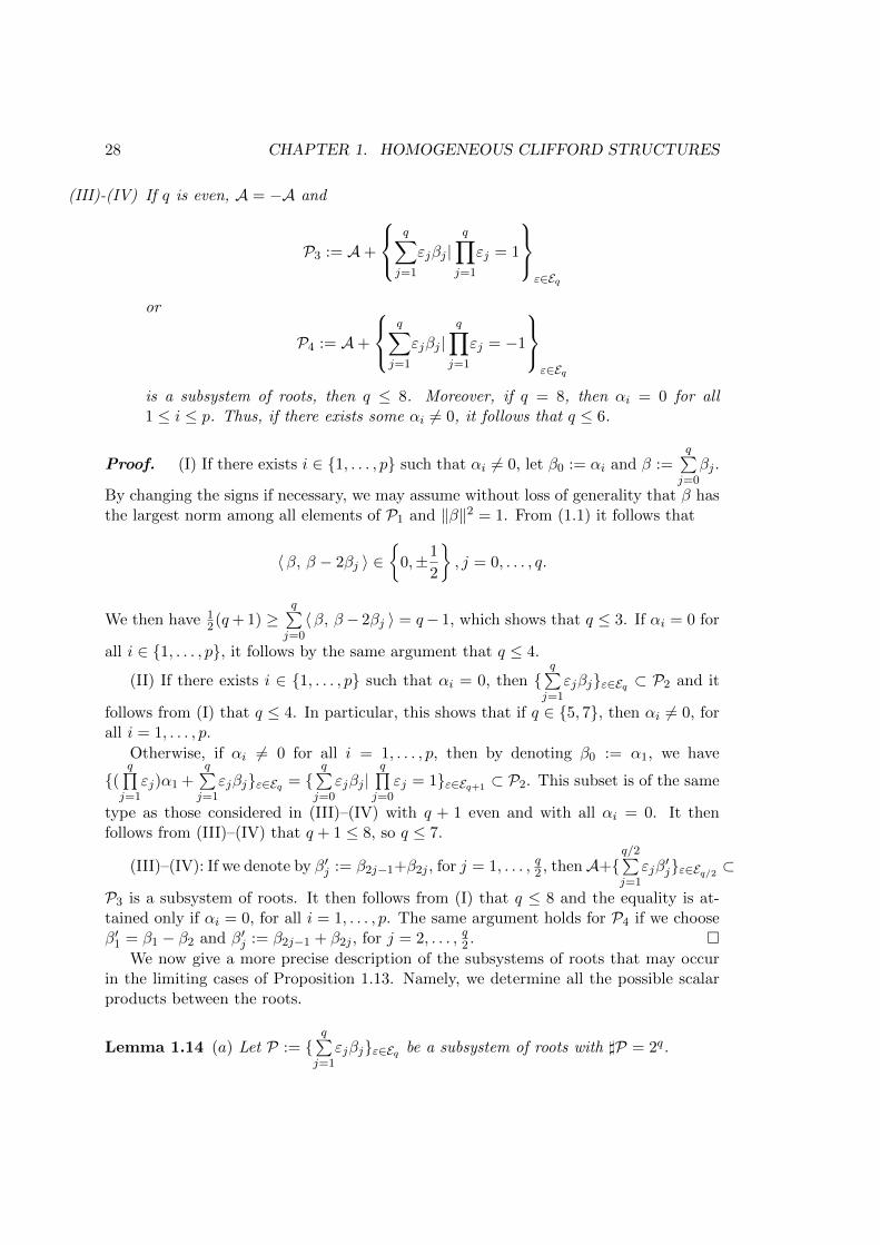
28 CHAPTER 1. HOMOGENEOUS CLIFFORD STRUCTURES
(III)-(IV) If q is even, A = −A and
P3 := A+
q∑j=1
εjβj |q∏j=1
εj = 1
ε∈Eq
or
P4 := A+
q∑j=1
εjβj |q∏j=1
εj = −1
ε∈Eq
is a subsystem of roots, then q ≤ 8. Moreover, if q = 8, then αi = 0 for all1 ≤ i ≤ p. Thus, if there exists some αi 6= 0, it follows that q ≤ 6.
Proof. (I) If there exists i ∈ 1, . . . , p such that αi 6= 0, let β0 := αi and β :=q∑j=0
βj .
By changing the signs if necessary, we may assume without loss of generality that β hasthe largest norm among all elements of P1 and ‖β‖2 = 1. From (1.1) it follows that
〈β, β − 2βj 〉 ∈
0,±1
2
, j = 0, . . . , q.
We then have 12(q+ 1) ≥
q∑j=0〈β, β− 2βj 〉 = q− 1, which shows that q ≤ 3. If αi = 0 for
all i ∈ 1, . . . , p, it follows by the same argument that q ≤ 4.
(II) If there exists i ∈ 1, . . . , p such that αi = 0, then q∑j=1
εjβjε∈Eq ⊂ P2 and it
follows from (I) that q ≤ 4. In particular, this shows that if q ∈ 5, 7, then αi 6= 0, forall i = 1, . . . , p.
Otherwise, if αi 6= 0 for all i = 1, . . . , p, then by denoting β0 := α1, we have
(q∏j=1
εj)α1 +q∑j=1
εjβjε∈Eq = q∑j=0
εjβj |q∏j=0
εj = 1ε∈Eq+1 ⊂ P2. This subset is of the same
type as those considered in (III)–(IV) with q + 1 even and with all αi = 0. It thenfollows from (III)–(IV) that q + 1 ≤ 8, so q ≤ 7.
(III)–(IV): If we denote by β′j := β2j−1+β2j , for j = 1, . . . , q2 , thenA+q/2∑j=1
εjβ′jε∈Eq/2 ⊂
P3 is a subsystem of roots. It then follows from (I) that q ≤ 8 and the equality is at-tained only if αi = 0, for all i = 1, . . . , p. The same argument holds for P4 if we chooseβ′1 = β1 − β2 and β′j := β2j−1 + β2j , for j = 2, . . . , q2 .
We now give a more precise description of the subsystems of roots that may occurin the limiting cases of Proposition 1.13. Namely, we determine all the possible scalarproducts between the roots.
Lemma 1.14 (a) Let P := q∑j=1
εjβjε∈Eq be a subsystem of roots with ]P = 2q.
1.3. THE ISOTROPY REPRESENTATION 29
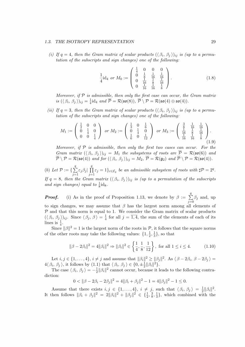
(i) If q = 4, then the Gram matrix of scalar products (〈βi, βj 〉)ij is (up to a permu-tation of the subscripts and sign changes) one of the following:
1
4id4 or M0 :=
14 0 0 00 1
8116
116
0 116
18
116
0 116
116
18
. (1.8)
Moreover, if P is admissible, then only the first case can occur, the Gram matrixis (〈βi, βj 〉)ij = 1
4 id4 and P = R(so(8)), P \ P = R(so(4)⊕ so(4)).
(ii) If q = 3, then the Gram matrix of scalar products (〈βi, βj 〉)ij is (up to a permu-tation of the subscripts and sign changes) one of the following:
M1 :=
12 0 00 1
4 00 0 1
4
or M2 :=
13 0 1
60 1
4 016 0 1
12
or M3 :=
38
116
116
116
18
116
116
116
18
.
(1.9)Moreover, if P is admissible, then only the first two cases can occur. For theGram matrix (〈βi, βj 〉)ij = M1 the subsystems of roots are P = R(so(6)) andP \ P = R(so(4)) and for (〈βi, βj 〉)ij = M2, P = R(g2) and P \ P = R(so(4)).
(b) Let P := q∑j=1
εjβj |q∏j=1
εj = 1ε∈Eq be an admissible subsystem of roots with ]P = 2q.
If q = 8, then the Gram matrix (〈βi, βj 〉)ij is (up to a permutation of the subscriptsand sign changes) equal to 1
8 id8.
Proof. (i) As in the proof of Proposition 1.13, we denote by β :=q∑j=0
βj and, up
to sign changes, we may assume that β has the largest norm among all elements ofP and that this norm is equal to 1. We consider the Gram matrix of scalar products(〈βi, βj 〉)ij . Since 〈βj , β 〉 = 1
4 for all j = 1, 4, the sum of the elements of each of itslines is 1
4 .Since ‖β‖2 = 1 is the largest norm of the roots in P, it follows that the square norms
of the other roots may take the following values: 1, 12 ,
13, so that
‖β − 2βi‖2 = 4‖βi‖2 ⇒ ‖βi‖2 ∈
1
4,1
8,
1
12
, for all 1 ≤ i ≤ 4. (1.10)
Let i, j ∈ 1, . . . , 4, i 6= j and assume that ‖βi‖2 ≥ ‖βj‖2. As 〈β − 2βi, β − 2βj 〉 =4〈βi, βj 〉, it follows by (1.1) that 〈βi, βj 〉 ∈ 0,±1
2‖βi‖2.
The case 〈βi, βj 〉 = −12‖βi‖
2 cannot occur, because it leads to the following contra-diction:
0 < ‖β − 2βi − 2βj‖2 = 4‖βi + βj‖2 − 1 = 4‖βj‖2 − 1 ≤ 0.
Assume that there exists i, j ∈ 1, . . . , 4, i 6= j, such that 〈βi, βj 〉 = 12‖βi‖
2.It then follows ‖βi + βj‖2 = 2‖βi‖2 + ‖βj‖2 ∈ 1
2 ,38 ,
13, which combined with the

30 CHAPTER 1. HOMOGENEOUS CLIFFORD STRUCTURES
restrictions (1.10) yield the following possible values: either ‖βi‖2 = ‖βj‖2 = 18 or
‖βi‖2 = 18 , ‖βj‖
2 = 112 . In both cases 〈βi, βj 〉 = 1
16 . Hence, all non-diagonal entriesare either 0 or 1
16 and since the sum of the elements of each line is equal to 14 , the
case ‖βj‖2 = 112 is excluded. It follows that each line of the Gram matrix (〈βi, βj 〉)ij
either has all non-diagonal entries equal to 0 and the diagonal term is 14 or two of
them are 116 , one is 0 and the diagonal term is 1
8 . In particular, ‖βi‖2 ∈ 14 ,
18, for all
1 ≤ i ≤ 4. Up to a permutation of the subscripts we may assume that ‖βi‖2 ≥ ‖βj‖2for all 1 ≤ i < j ≤ 4. The following two cases may occur: either ‖β1‖2 = ‖β2‖2 = 1
4 or‖β1‖2 = 1
4 and ‖β2‖2 = 18 .
In the first case at most one non-diagonal term may be 116 , showing that they must
all be equal to 0. This contradicts 〈βi, βj 〉 = 12‖βi‖
2 6= 0. In the second case, since wehave one non-diagonal term equal to 1
16 , we must have another one and then ‖β3‖2 =‖β4‖2 = 1
8 . Hence, the corresponding Gram matrix is equal to M0 defined by (1.8).
The subsystem of roots corresponding to the matrix M0 is not admissible, sincethe necessary criterion given by Lemma 1.6 is not fulfilled: the set βii=1,4 is linearlyindependent (since the Gram matrix is invertible) and β, β − 2β2 are two roots of thesubsystem, which have different norms ‖β−2β2‖2 = 1
2 = 12‖β‖
2 and are not orthogonal:〈β, β − 2β2 〉 = 1
2 .
The only case left is when βii=1,4 is an orthonormal system. In this case the newroots obtained by considering all possible reflections are the roots ±2βii=1,4, whichare of the same norm and orthogonal to each other and thus build the system of roots
of su(2) ⊕ su(2) ⊕ su(2) ⊕ su(2). Then the minimal set of roots is P = ±4∑j=1
εjβj ∪
±2βii=1,4, which is the system of roots of so(8), proving (i).
(ii) If q = 3, we assume as above that β := β1 + β2 + β3 is the element of Pof maximal norm and ‖β‖2 = 1. From (1.1) it follows that 〈β, β − 2βi 〉 ∈ 0,±1
2,for all i = 1, 3, yielding that 〈β, βi 〉 ∈ 1
2 ,14 ,
34. Since 1 = ‖β‖2 =
∑3i=1〈βi, β 〉,
the only possible values (up to a permutation of the subscripts) are 〈β1, β 〉 = 12 and
〈β2, β 〉 = 〈β3, β 〉 = 14 . Then, from ‖β − 2βi‖2 ∈ 1, 1
2 ,13, it follows that
‖β1‖2 ∈
1
2,3
8,1
3
, ‖β2‖2, ‖β3‖2 ∈
1
4,1
8,
1
12
. (1.11)
Since 〈β, β − 2β1 〉 = 0 and 〈β, β − 2β2 〉 = 〈β, β − 2β3 〉 = 12 , we obtain the following
expressions for the scalar products:
2〈β2, β3 〉 = ‖β1‖2 − ‖β2‖2 − ‖β3‖2, (1.12)
2〈β1, β2 〉 =1
2+ ‖β3‖2 − ‖β1‖2 − ‖β2‖2, (1.13)
2〈β1, β3 〉 =1
2+ ‖β2‖2 − ‖β1‖2 − ‖β3‖2. (1.14)
The other conditions for the scalar products of roots in P obtained from (1.1) are:〈β − 2βi, β − 2βj 〉 ∈ 0,±1
2 max(‖β − 2βi‖2, ‖β − 2βj‖2), for all 1 ≤ i < j ≤ 3, which
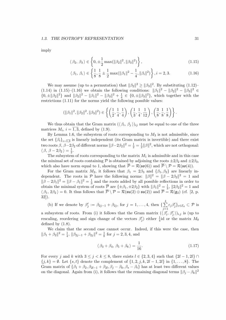
1.3. THE ISOTROPY REPRESENTATION 31
imply
〈β2, β3 〉 ∈
0,±1
2max(‖β2‖2, ‖β3‖2)
, (1.15)
〈β1, βi 〉 ∈
1
8,1
8± 1
2max(‖β1‖2 −
1
4, ‖βi‖2)
, i = 2, 3. (1.16)
We may assume (up to a permutation) that ‖β2‖2 ≥ ‖β3‖2. By substituting (1.12)–(1.14) in (1.15)–(1.16) we obtain the following conditions: ‖β1‖2 − ‖β2‖2 − ‖β3‖2 ∈0,±‖β2‖2 and ‖β2‖2 − ‖β1‖2 − ‖β3‖2 + 1
4 ∈ 0,±‖β3‖2, which together with therestrictions (1.11) for the norms yield the following possible values:
(‖β1‖2, ‖β2‖2, ‖β3‖2) ∈(
1
2,1
4,1
4
),
(1
3,1
4,
1
12
),
(3
8,1
8,1
8
).
We thus obtain that the Gram matrix (〈βi, βj 〉)ij must be equal to one of the threematrices Mi, i = 1, 3, defined by (1.9).
By Lemma 1.6, the subsystem of roots corresponding to M3 is not admissible, sincethe set βii=1,3 is linearly independent (its Gram matrix is invertible) and there exist
two roots β, β−2β2 of different norms ‖β−2β2‖2 = 12 = 1
2‖β‖2, which are not orthogonal:
〈β, β − 2β2 〉 = 12 .
The subsystem of roots corresponding to the matrix M1 is admissible and in this casethe minimal set of roots containing P is obtained by adjoining the roots ±2β2 and ±2β3,which also have norm equal to 1, showing that P = R(so(6)) and P \ P = R(so(4)).
For the Gram matrix M2, it follows that β1 = 2β3 and β1, β2 are linearly in-dependent. The roots in P have the following norms: ‖β‖2 = ‖β − 2β2‖2 = 1 and‖β − 2β1‖2 = ‖β − β1‖2 = 1
3 and the roots added by all possible reflections in order toobtain the minimal system of roots P are ±β1,±2β2 with ‖β1‖2 = 1
3 , ‖2β2‖2 = 1 and〈β1, 2β2 〉 = 0. It thus follows that P \ P = R(su(2)⊕ su(2)) and P = R(g2) (cf. [2, p.32]).
(b) If we denote by β′j := β2j−1 + β2j , for j = 1, . . . , 4, then 4∑j=1
εjβ′jε∈E4 ⊂ P is
a subsystem of roots. From (i) it follows that the Gram matrix (〈β′i, β′j 〉)i,j is (up to
rescaling, reordering and sign change of the vectors β′j) either 14 id or the matrix M0
defined by (1.8).We claim that the second case cannot occur. Indeed, if this were the case, then
‖β1 + β2‖2 = 14 , ‖β2j−1 + β2j‖2 = 1
8 for j = 2, 3, 4, and
〈β3 + β4, β5 + β6 〉 =1
16. (1.17)
For every j and k with 3 ≤ j < k ≤ 8, there exists l ∈ 2, 3, 4 such that 2l − 1, 2l ∩j, k = ∅. Let s, t denote the complement of 1, 2, j, k, 2l − 1, 2l in 1, . . . , 8. TheGram matrix of β1 + β2, β2l−1 + β2l, βj − βk, βs − βt has at least two different valueson the diagonal. Again from (i), it follows that the remaining diagonal terms ‖βj−βk‖2

32 CHAPTER 1. HOMOGENEOUS CLIFFORD STRUCTURES
and ‖βs − βt‖2 must both be equal to 18 . Thus, ‖βj − βk‖2 = 1
8 for all 3 ≤ j < k ≤ 8.By the same argument we also obtain ‖βj + βk‖2 = 1
8 for all 3 ≤ j < k ≤ 8. Thus,〈βj , βk 〉 = 0 for all 3 ≤ j < k ≤ 8, contradicting (1.17).
This shows that the vectors β′j are mutually orthogonal. Applying this to differentpartitions of the set 1, . . . , 8 into four pairs we get that βj +βk is orthogonal to βs+βtfor all mutually distinct subscripts j, k, s and t. This clearly implies that 〈βi, βj 〉 = 0for all i 6= j. It then also follows that ‖βj‖2 = 1
8 , for j = 1, . . . , 8, proving (b).
1.4 Homogeneous Clifford Structures of high rank
A direct consequence of Propositions 1.12 and 1.13 is the following upper bound for therank of a homogeneous Clifford structure:
Theorem 1.15 The rank r of any even homogeneous Clifford structure on a homoge-neous compact manifold G/H of non-vanishing Euler characteristic is less or equal to 16.More precisely, the following restrictions hold for the rank depending on its 2-valuation:
(I) If r is odd, then r ∈ 3, 5, 7, 9.
(II) If r ≡ 2 mod 4, then r ∈ 2, 6, 10.
(III) If r ≡ 4 mod 8, then r ∈ 4, 12.
(IV) If r ≡ 0 mod 8, then r ∈ 8, 16.
Proof. We only need to show that in case (II), the rank r is strictly less than 14.This will be done in the proof of Theorem 1.16 (II).
We further describe the manifolds which occur in the limiting cases for the upperbounds in Theorem 1.15.
Theorem 1.16 The maximal rank r of an even homogeneous Clifford structure for eachof the types (I)-(IV) and the corresponding compact homogeneous manifolds M = G/H(with rk(G) = rk(H)) carrying such a structure are the following:
(I) r = 9 and M is the Cayley projective space OP2 = F4/Spin(9).
(II) r = 10 and M = (C⊗O)P2 = E6/(Spin(10)×U(1)/Z4).
(III) r = 12 and M = (H⊗O)P2 = E7/Spin(12) · SU(2).
(IV) r = 16 and M = (O⊗O)P2 = E8/(Spin(16)/Z2).
Proof. Let M = G/H (rk(G) = rk(H)) carry a homogeneous Clifford structure ofrank r.
(I) If r is odd, r = 2q + 1, then it follows from Theorem 1.15 (I) that r ≤ 9.
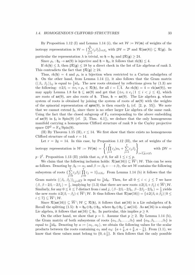
1.4. HOMOGENEOUS CLIFFORD STRUCTURES 33
By Proposition 1.12 (I) and Lemma 1.14 (i), the set W := W(m) of weights of the
isotropy representation is W = q∑j=1
εjβjε∈Eq with ]W = 2q and R(so(8)) ⊆ R(g). In
particular the representation λ is trivial, so h = h2 and ]R(g) ≥ 24.
Since ρ∗ : h2 → so(9) is injective and h = h2, it follows that rk(h) ≤ 4.
If rk(h) ≤ 3, then ]R(g) ≤ 18 by a direct check in the list of Lie algebras of rank 3.This contradicts the fact that ]R(g) ≥ 24.
Thus, rk(h) = 4 and ρ∗ is a bijection when restricted to a Cartan subalgebra ofh. On the other hand, from Lemma 1.14 (i), it also follows that the Gram matrix(〈βi, βj 〉)ij is equal to 1
4 id4. The new roots obtained by reflections given by (1.3) arethe following: ±2βi = ±ei ρ∗ ∈ R(h), for all i = 1, 4. As rk(h) = 4 = rk(so(9)), wemay apply Lemma 1.8 for h ⊆ so(9) and get that ±ei ± ej | 1 ≤ i < j ≤ 4, whichare roots of so(9), are also roots of h. Thus, h = so(9). The Lie algebra g, whosesystem of roots is obtained by joining the system of roots of so(9) with the weightsof the spinorial representation of spin(9), is then exactly f4 (cf. [2, p. 55]). We notethat we cannot extend f4, since there is no other larger Lie algebra of the same rank.Using the fact that the closed subgroup of F4 corresponding to the above embeddingof so(9) in f4 is Spin(9) (cf. [2, Thm. 6.1]), we deduce that the only homogeneousmanifold carrying a homogeneous Clifford structure of rank 9 is the Cayley projectivespace OP2 = F4/Spin(9).
(II) By Theorem 1.15 (II), r ≤ 14. We first show that there exists no homogeneousClifford structure of rank r = 14.
Let r = 2q = 14. In this case, by Proposition 1.12 (II), the set of weights of the
isotropy representation is W := W(m) =
(
7∏j=1
εj)αi +7∑j=1
εjβj
i=1,p,ε∈E7
with ]W =
p · 27. Proposition 1.13 (II) yields that αi 6= 0, for all 1 ≤ i ≤ p.We claim that the following inclusion holds: R(so(16)) ⊆ W \W. This can be seen
as follows. Denoting by β0 := α1 and β := β0 + · · ·+β7, the setW contains the following
subsystem of roots 7∑j=0
εjβj |7∏j=0
εj = 1ε∈E8 . From Lemma 1.14 (b) it follows that the
Gram matrix (〈βi, βj 〉)i,j=0,7 is equal to 18 id8. Then, for all 0 ≤ i < j ≤ 7 we have
〈β, β−2βi−2βj 〉 = 12 , implying by (1.3) that there are new roots ±2(βi+βj) ∈ W\W.
Similarly, for any 0 ≤ k ≤ 7 distinct from i and j, 〈β−2βi−2βk, β−2βj−2βk 〉 = 12 yields
the new roots ±2(βi−βj) ∈ W \W. It thus follows that R(so(16)) = ±2(βi±βj) | 0 ≤i ≤ 7 ⊆ W \W.
Since R(so(16)) ⊆ W \ W ⊆ R(h), it follows that so(16) is a Lie subalgebra of h.Recall the splitting (1.5): h = h0⊕h1⊕h2, where h0⊕h2 ⊆ so(14). As so(16) is a simpleLie algebra, it follows that so(16) ⊆ h1. In particular, this implies p ≥ 8.
On the other hand, we show that p = 1. Assume that p ≥ 2. By Lemma 1.14 (b),the Gram matrix of both subsystems of roots α1, β1, . . . , β7 and α2, β1, . . . , β7 isequal to 1
8 id8. Denoting by a := 〈α1, α2 〉, we obtain the following values for the scalarproducts between the roots containing α1 and α2: a+ 7
8 , a+ 38 , a−
18. From (1.1), we
know that these values must belong to 0,±12. It then follows that the only possible
34 CHAPTER 1. HOMOGENEOUS CLIFFORD STRUCTURES
value for a = 〈α1, α2 〉 is −38 . This leads to a contradiction by computing the following
norm: ‖α1 + α2‖2 = −12 < 0.
Thus, the case r = 14 is not possible.
Now, for rank r = 10 = 2q, by Proposition 1.12 (II), the set of weights of the isotropy
representation is W :=W(m) = (5∏j=1
εj)αi +5∑j=1
εjβji=1,p,ε∈E5 with ]W = p · 25. From
Proposition 1.13 (II), it then follows that αi 6= 0, for all 1 ≤ i ≤ p. We will further showthat p = 1 and the following inclusions hold: R(spin(10)⊕ u(1)) ⊆ W \W, R(e6) ⊆ W.
Let β0 := α1 and β′j := β2j + β2j+1, for j = 0, 1, 2. Then ∑2
j=0 εjβ′j ⊂ W
is an admissible subsystem of roots. By Lemma 1.14 (ii), the Gram matrix B′ :=(〈β′i, β′j 〉)i,j=0,2 is one of the three matrices in (1.9). We may assume that β′0 is ofmaximal norm and equal to 1, so that the possible Gram matrices B′ are normalized asfollows:
M1 :=
1 0 00 1
2 00 0 1
2
,M2 :=
1 0 12
0 34 0
12 0 1
4
,M3 :=
1 16
16
16
13
16
16
16
13
. (1.18)
We first note that the norm of β :=∑5
j=0 βj , which is equal to the sum of all elements
of the matrix B′, may take the following values: ‖β‖2 = 2 for M1, ‖β‖2 = 3 for M2,‖β‖2 = 8
3 for M3. We will show that the last two cases cannot occur.
Let us first assume that B′ = M2. In this case β′0 = 2β′2, i.e. β0 + β1 = 2(β4 + β5).Considering now another pairing by permuting the subscripts 2, 3, 4, 5, we get a Grammatrix which must also be equal to M2, since ‖β‖2 does not change. We may thusassume that β0 + β1 = 2(β2 + β4) and is furthermore equal either to 2(β2 + β5) or to2(β3 + β4). In both cases it follows that there exists i 6= j ∈ 2, 3, 4, 5, such thatβi = βj . Then, for any k 6= i, j, the roots β − 2βi − 2βk, β − 2βj − 2βk ∈ W are equal,which contradicts ]W = p · 25. Thus, B′ 6= M2.
Let us now assume that the Gram matrix B′ is equal to M3. Then ‖β‖2 = 83 and
since this is the maximal norm, it follows that for any other possible pairing of thevectors βj , the corresponding Gram matrix is either M1 or M3 (because the sum of allelements of M2 is 3 > 8
3).
We consider as above other pairings by permuting the subscripts 2, 3, 4, 5. Againby Lemma 1.14 (ii), it follows that the corresponding Gram matrix is one of the matricesin (1.18) and, since ‖β‖2 does not change, it must also be equal to M3. In particular,we have:
‖βi + βj‖2 =1
3, (1.19)
〈βi + βj , βk + βl 〉 =1
6, (1.20)
for any permutation (i, j, k, l) of (2, 3, 4, 5).
Consider now the following pairings of the vectors βj :
β′′0 := β0 + β1, β′′1 := ±(βi − βj), β′′2 := ±(βk − βl),
1.4. HOMOGENEOUS CLIFFORD STRUCTURES 35
where (i, j, k, l) is any permutation of (2, 3, 4, 5) and in each case the signs for β′′1 andβ′′2 are chosen such that
‖β′′0 + β′′1 + β′′2‖2 = max‖β′′0 ± β′′1 ± β′′2‖2.
Then ∑2
j=0 εjβ′′j is a subsystem of roots of W and by the same argument as above its
Gram matrix B′′ := (〈β′′i , β′′j 〉)i,j=0,2 is either M1 or M3.
Since ‖β′′0‖2 = 1, it follows that in both cases the norms of the other two vectors areequal: ‖β′′1‖2 = ‖β′′2‖2, i.e. ‖βi − βj‖2 = ‖βk − βl‖2 ∈ 1
2 ,13. By (1.19), we then obtain
for any i, j ∈ 2, 3, 4, 5 that 〈βi, βj 〉 = 14(‖βi + βj‖2 − ‖βi − βj‖2) ∈ 0,− 1
24. It thenfollows that 〈βi + βj , βk + βl 〉 < 0, for any permutation (i, j, k, l) of (2, 3, 4, 5), whichcontradicts (1.20). Thus, B′ 6= M3.
The only possibility left is B′ = M1. Then ‖β‖2 = 2 and since it is the element ofmaximal norm, it follows that for any other pairing of the vectors βj , the correspondingGram matrix is also equal to M1. We then have B′ = B′′ = M1, which implies:
〈β0 + β1, βi ± βj 〉 = 0, (1.21)
‖βi + βj‖2 = ‖βi − βj‖2 =1
2, (1.22)
〈βi + βj , βk + βl 〉 = 〈βi − βj , βk − βl 〉 = 0, (1.23)
for any permutation (i, j, k, l) of (2, 3, 4, 5). From (1.21) it follows that 〈β0 +β1, βi 〉 = 0for all 2 ≤ i ≤ 5. From (1.23) it follows that 〈βi, βj 〉 = 0, for 2 ≤ i < j ≤ 5 and thenfrom (1.22) we obtain ‖βi‖2 = 1
4 , for 2 ≤ i ≤ 5.For pairings of the following form β0 − β1, βi − βj , βk + βl, where again (i, j, k, l) is
a permutation of (2, 3, 4, 5), the corresponding Gram matrix must also be equal to M1.Since ‖βi±βj‖2 = 1
4 , for all 2 ≤ i < j ≤ 5, it follows that ‖β0−β1‖2 = 1, so 〈β0, β1 〉 = 0.By the above argument applied to this pairing, it follows a similar relation, namely:〈β0 − β1, βi ± βj 〉 = 0, which together with (1.21) yields 〈β0, βi 〉 = 〈β1, βj 〉 = 0, for2 ≤ i ≤ 5. Thus, the Gram matrix (〈βi, βj 〉)0≤i,j≤5 is diagonal with ‖β0‖2 + ‖β1‖2 = 1and ‖βi‖2 = 1
4 , for 2 ≤ i ≤ 5.The second element in the decreasing order of the set ‖βi + βj‖2 | 0 ≤ i < j ≤ 5
must be, up to a permutation of 0 and 1, of the form β0 + βk, for some 2 ≤ k ≤ 5. Bytaking now, for instance, a pairing with first element equal to β0 + βk, it follows thatits Gram matrix is equal to M1 and by the same argument as above ‖β1‖2 = 1
4 and,consequently, ‖β0‖2 = 3
4 . Since we allowed permutations, we have to consider two cases:‖α1‖2 ∈ 3
4 ,14.
If ‖α1‖2 = 14 , we may assume that ‖β1‖2 = 3
4 and ‖βi‖2 = 14 , for all 2 ≤ i ≤ 5. Since
the Gram matrix is now completely known, we compute the scalar products between theroots inW and by (1.3) we obtain: ±2(α1±βi),±2(βj±βi)| 2 ≤ i < j ≤ 5 ⊆ W\W ⊆R(h). Considering the orthogonal decomposition (1.5) of h, it follows by Lemma 1.9 (ii)that there is a k ∈ 0, 1, 2 such that ±2(α1±βi),±2(βj±βi)| 2 ≤ i < j ≤ 5 ⊆ R(hk).Since α1 ∈ h0⊕ h1 and βi ∈ h0⊕ h2, for 1 ≤ i ≤ 5, the only possible value is k = 0. Thisimplies that so(10) ⊆ h0 and thus p ≥ 5. We show that this is not possible.

36 CHAPTER 1. HOMOGENEOUS CLIFFORD STRUCTURES
Assuming that p ≥ 2 and computing the scalar products between α1 + β1 + · · ·+ β5
and α2 + β1 ± (β2 + β3) ± (β4 + β5), we get the following values a + 74 , a + 3
4 , a −14,
where a := 〈α1, α2 〉. By (1.1), we know that a + 74 , a + 3
4 , a −14 ⊆ 0,±1. Hence,
a = −34 , which implies that ‖α1 +α2‖2 = −1. Thus, the case ‖α1‖2 = 1
4 may not occur.We then have ‖α1‖2 = 3
4 and ‖βi‖2 = 14 , for 1 ≤ i ≤ 5. Again by computing
all possible scalar products, we produce by (1.3) the new roots ±2(βi ± βj)| 1 ≤ i <j ≤ 5 ⊆ R(h). By Lemma 1.9 (i) and (ii), there exists a k ∈ 0, 1, 2 such that±2(βi±βj)| 1 ≤ i < j ≤ 5 are all roots of one of the components hk of the orthogonalsplitting h = h0 ⊕ h1 ⊕ h2 given by (1.5). As βi ∈ h0 ⊕ h2 for 1 ≤ i ≤ 5, it follows thatk ∈ 0, 2. Thus, R(hk) contains the whole system of roots of so(10). On the otherhand, h0⊕h2 ⊆ so(10). Hence, there are two possibilities: either h0 = so(10) and h2 = 0or h0 = 0 and h2 = so(10).
Let us first note that if p ≥ 2, then 〈αi, αj 〉 = −1, for all 1 ≤ i < j ≤ p. Bycomputing the scalar products between the different roots containing αi, respectivelyαj , we obtain the following values: a := 〈αi, αj 〉 ∈ a+ 5
4 , a+ 14 , a−
34, which by (1.1)
must be contained into 0,±1. Hence, the only possible value is a = −14 .
In the first case, h0 = so(10) implies that p ≥ 5, which by the above remark leads tothe following contradiction: ‖α1 + · · ·+ α5‖2 = −5
4 < 0.Thus, the second case h2 = so(10) and h0 = 0 must hold. We show that p = 1.
Assuming p ≥ 2, we compute 〈α1 + β1 + · · ·+ β5, α2 + β1 − β2 − · · · − β5 〉 = −1, whichby (1.3) yields the new mixed root α1 + α2 + 2β1 ∈ R(h), contradicting Lemma 1.9 (i)(since α1 + α2 ∈ h1 and β1 ∈ h2). Thus, p = 1 and h1 = u(1).
Concluding, it follows that h = so(10)⊕u(1). Therefore,R(g) =W∪R(so(10)⊕u(1)),is exactly the system of roots of e6 (cf. [2, p. 57]), hence g = e6. From [2, Thm.6.1], the Lie subgroup of E6 corresponding to the above embedding of so(10) ⊕ u(1)in e6 is Spin(10) × U(1)/Z4, showing that the only homogeneous manifold carryinga homogeneous Clifford structure of rank r = 10 is the exceptional symmetric space(C⊗O)P2 = E6/(Spin(10)×U(1)/Z4).
(III) By Theorem 1.15 (III), the maximal rank in this case is r = 12. For r = 12 = 2q,from Proposition 1.12 (III), there exist A := α1, . . . , αp and G := γ1, . . . , γp′ in t∗
with A = −A and G = −G such that the set of weights of the isotropy representation isgiven by:
W(m) = A+
6∑j=1
εjβj |6∏j=1
εj = 1
ε∈E6
⋃G +
6∑j=1
εjβj |6∏j=1
εj = −1
ε∈E6
with ]W = (p+ p′) · 25, where one of p or p′ might vanish, but the vectors αi and γi areall non-zero.
Assume p 6= 0 (otherwise the same argument applies for p′ 6= 0 by changing the signof β1) and denote by
W := A+
6∑j=1
εjβj |6∏j=1
εj = 1
ε∈E6
,
1.4. HOMOGENEOUS CLIFFORD STRUCTURES 37
which is an admissible subsystem of roots as in Proposition 1.13 (III), with ]W = p · 25.
We claim that the following inclusions hold: R(so(12)⊕su(2)) ⊆ W\W, R(e7) ⊆ W.
Let us consider all the subsystems of roots of the following form ∑4
j=1 εjβ′j ⊂ W,
where β′1 = α1, β′2 = β1 ± β2, β′3 = β3 ± β4, β′4 = β5 ± β6 and such that the numberof minus signs in β′2, β
′3 and β′4 is even, as well as all the other subsystems obtained by
permuting the subscripts 1, . . . , 6 of the vectors βj .
By Lemma 1.14 (i), the Gram matrix (〈β′i, β′j 〉)i,j is either 14 id4 or the matrix M0
defined by (1.8). We further show that the second case can not occur. Indeed, if thiswere the case, then at least two of the norms ‖β′2‖2, ‖β′3‖2 and ‖β′4‖2 are equal and afterreordering, rescaling and sign change of the vectors βj we may assume β′2 = β1 + β2,β′3 = β3 + β4, β′4 = β5 + β6 and ‖β′3‖2 = ‖β′4‖2 = 1
8 , 〈β′3, β′4 〉 = 116 . If we denote by
β′′j := β′j , j = 1, 2 and β′′3 = β3 − β4, β′′4 = β5 − β6, then ∑4
j=1 εjβ′′j ⊂ W is also a
subsystem of roots. Since ‖β′′1‖2, ‖β′′2‖2 = 14 ,
18, it follows again by Lemma 1.14 (i)
that the Gram matrix (〈β′′i , β′′j 〉)i,j is equal to M0 defined by (1.8), so that ‖β′′4‖2 =
‖β′′3‖2 = 18 = ‖β′3‖2 = ‖β′4‖2. Thus, ‖β1 + β2‖2 = 1
4 , ‖β2j−1 + β2j‖2 = 18 for j = 2, 3, 4,
and
〈β3 + β4, β5 + β6 〉 =1
16. (1.24)
For every 3 ≤ j < k ≤ 8, there exists l ∈ 2, 3, 4 such that 2l− 1, 2l ∩ j, k = ∅. Lets, t denote the complement of 1, 2, j, k, 2l− 1, 2l in 1, . . . , 8. The Gram matrix ofβ1 + β2, β2l−1 + β2l, βj − βk, βs − βt has at least two different values on the diagonal.By Lemma 1.14 (i) again, the remaining diagonal terms ‖βj − βk‖2 and ‖βs − βt‖2 areboth equal to 1
8 . Thus ‖βj − βk‖2 = 18 for 3 ≤ j < k ≤ 8, and similarly ‖βj + βk‖2 = 1
8for 3 ≤ j < k ≤ 8. Thus 〈βj , βk 〉 = 0 for all 3 ≤ j < k ≤ 8, contradicting (1.24).
It then follows that the Gram matrix of any subsystem of roots ∑4
j=1 εjβ′j as
above is (〈β′i, β′j 〉)i,j = 14 id4. In particular, this shows that for any 1 ≤ i < j ≤ 6,
‖βi + βj‖2 = ‖βi − βj‖2 = 14 , and 〈α1, βi + βj 〉 = 〈α, βi − βj 〉 = 0, implying that
〈βi, βj 〉 = 0 and 〈βi, α1 〉 = 0. For any k 6= i, j we also have ‖βi+βk‖2 = ‖βj+βk‖2 = 14 ,
which then yields ‖βi‖2 = 18 for 1 ≤ i ≤ 6. Denoting by β′ :=
∑4i=1 β
′i, we compute
〈β′ − 2β′i, β′ 〉 = 1
2 , for 1 ≤ i ≤ 4. By (1.3) we obtain the new roots ±2β′i ∈ W \ W.Since the argument is true for any such subsystem of roots, we have the new roots±2α1,±2(βi±βj)| 1 ≤ i < j ≤ 6 ⊆ W\W, which, by the above orthogonality relations,build the system of roots of so(12) ⊕ su(2). It thus follows that so(12) ⊕ su(2) ⊆ h.Furthermore, R(so(12)⊕ su(2)) ∪W = R(e7) (cf. [2, p. 56]), showing that e7 ⊆ g.
We claim that p = 1. Assuming that p ≥ 2, we consider α2 ∈ A\±α1. The previousargument also shows that 〈βi, α2 〉 = 0 for all 1 ≤ i ≤ 6. Denoting by a := 〈α1, α2 〉,the scalar products between β := α1 +
∑6j=1 βj and α2± (β1 +β2)± (β3 +β4)± (β5 +β6)
take four possible values: a ± 34 , a ±
14, thus contradicting (1.1), which only allows 3
different values for these scalar products. Hence, p = 1, and similarly p′ ≤ 1.
We further prove that p′ = 0. Assuming the contrary, there exists γ1 6= 0 in G. Thesame arguments as before show that 〈βi, γ1 〉 = 0 for 1 ≤ i ≤ 6 and ‖γ1‖2 = 1
4 . Denoting
by a := 〈α1, α2 〉, the set of scalar products between the unit vectors α1 +∑6
j=1 βj and
γ1 + β1 − β2 ± (β3 + β4) ± (β5 + β6) equals a, a ± 12. By (1.1), one has necessarily
38 CHAPTER 1. HOMOGENEOUS CLIFFORD STRUCTURES
a = 0, i.e. α1 ⊥ γ1. We then denote by β7 := 12(α1 + β1) and β8 := 1
2(α1 − β1). Theabove relations show that 〈βi, βj 〉 = 0, ‖βi‖2 = 1
8 for 1 ≤ i < j ≤ 8 and
W(m) =
8∑j=1
εjβj |8∏j=1
εj = 1
ε∈E8
.
Let β :=∑8
i=1 βi. Since 〈β, β− 2βi− 2βj 〉 = 12 for i 6= j and 〈β− 2βi− 2βk, β− 2βj −
2βk 〉 = 12 for i 6= j 6= k 6= i, by (1.3) we obtain that ±2(βi ± βj)| 1 ≤ i < j ≤ 8 ∈
W \W ⊂ R(h). This is exactly the system of roots of so(16). Thus, so(16) ⊆ h. Sinceso(16) is simple, the restriction to so(16) of the Clifford morphism ρ∗ : h→ so(12) mustvanish. Moreover, the restriction to so(16) of the representations λ± from Lemma 1.11vanish, too. Indeed, p = p′ = 1 and K = H so their complex dimensions equal 2. Thusthe isotropy representation of G/H would vanish on so(16) ⊂ h, a contradiction.
As p′ = 0, Lemma 1.11 shows that the isotropy representation can be written m =µ+ ⊗H λ+, so as in (1.5) we can write
h = h0 ⊕ h1 ⊕ h2 (1.25)
with h1 := ker(ρ∗), h2 := ker(λ+) and h0 = (h1 ⊕ h2)⊥. Since p = 1, it follows thath0 ⊕ h1 ⊆ su(2). On the other hand, h0 ⊕ h2 ⊆ so(12) and we have proved thatso(12)⊕ su(2) ⊆ h. Hence, we obtain h2 = so(12), h0 = 0 and h1 = su(2). In particular,we have h = so(12) ⊕ su(2), and R(g) = W(m) ⊕R(h) is isometric to the root systemof e7 (cf. [2, p. 56]). We conclude that M = E7/Spin(12) · SU(2) by [2, Thm 6.1].
(IV) For r = 16 = 2q, it follows from Proposition 1.12 (IV) and Proposition 1.13(III)-(IV) (for the extremal case q = 8) that (up to a sign change for one of the vectorsβi) p = 1, p′ = 0 and the set of weights of the isotropy representation is given by:
W(m) =
8∑j=1
εjβj |8∏j=1
εj = 1
ε∈E8
.
By Lemma 1.14 (b) it follows that the Gram matrix (〈βi, βj 〉)ij is equal to 18 id8.
Thus, all roots in W have norm 1 and 〈β, βi 〉 = 18 , where β :=
∑8i=1 βi. This yields
the following values for the scalar products for all i, j and k mutually distinct : 〈β, β−2βi − 2βj 〉 = 〈β − 2βi − 2βj , β − 2βi − 2βk 〉 = 1
2 and all other scalar products of rootsin W are 0. The new roots we obtain by (1.3) are then ±2(βi ± βj)| 1 ≤ i < j ≤ 8,which build the system of roots of so(16). Thus, so(16) ⊆ h. As p = 1 and p′ = 0 andso(16) ⊆ h, it follows with the notation from (1.25) that so(16) ⊆ h2. On the other hand,ρ∗ maps h0⊕h2 one-to-one into so(16) and thus we must have equality: h0⊕h2 = so(16).Consequently, R(g) = R(so16) ∪W is isometric to the system of roots of e8 (cf. [2, p.56]), showing that g = e8 and M = E8/(Spin(16)/Z2) by [2, Thm 6.1].
As already mentioned in Section 1, similar methods could be used to examine theremaining cases r ≤ 8. However, the arguments tend to be much more intricate as fastas the rank decreases. In order to keep this paper at a reasonable length, we have thusdecided to limit our study to the extremal cases of Theorem 1.15.

Bibliography
[1] J. Adams, Lectures on Lie groups, The University of Chicago Press, Chicago (1969).
[2] J. Adams, Lectures on exceptional Lie groups, Z. Mahmud and M. Mimura, eds.,Chicago Lectures in Mathematics, University of Chicago Press, Chicago (1996).
[3] A. Gray, Spaces of constancy of curvature operators, Proc. Amer. Math. Soc. 17(1966), 897–902.
[4] D. Joyce, Manifolds with many complex structures, Q. J. Math. Oxford Ser. (2) 46(1995), 169–184.
[5] B. Lawson, M.-L. Michelson, Spin Geometry, Princeton University Press, Princeton,NJ, 1989.
[6] A. Moroianu, U. Semmelmann, Clifford structures on Riemannian manifolds, Adv.Math. 228 (2011), 940–967.
[7] B. Rosenfeld, Geometrical interpretation of the compact simple Lie groups of theclass E (Russian), Dokl. Akad. Nauk. SSSR 106 (1956), 600–603.
[8] H. Samelson, Notes on Lie Algebras, Springer, Berlin (1990).
39

40 BIBLIOGRAPHY
Chapter 2
Homogeneous almostquaternion-Hermitian manifolds
Andrei Moroianu, Mihaela Pilca and Uwe Semmelmann
Abstract. An almost quaternion-Hermitian structure on a Riemannian manifold (M4n, g)is a reduction of the structure group of M to Sp(n)Sp(1) ⊂ SO(4n). In this paper we showthat a compact simply connected homogeneous almost quaternion-Hermitian manifold of non-vanishing Euler characteristic is either a Wolf space, or S2 × S2, or the complex quadricSO(7)/U(3).
2010 Mathematics Subject Classification: Primary: 53C30, 53C35, 53C15. Secondary: 17B22
Keywords: Quaternion-Hermitian structures, homogeneous spaces, root systems, Cliffordstructures.
2.1 Introduction
The notion of (even) Clifford structures on Riemannian manifolds was introduced in[12]. Roughly speaking, a rank r (even) Clifford structure on M is a rank r Euclideanbundle whose (even) Clifford algebra bundle acts on the tangent bundle of M . Forr = 3, an even Clifford structure on M is just an almost quaternionic structure, i.e. arank 3 sub-bundle Q of the endomorphism bundle End (TM) locally spanned by threeendomorphisms I, J,K satisfying the quaternionic relations
I2 = J2 = K2 = −id, IJ = K.
If moreover Q ⊂ End−(TM) (or, equivalently, if I, J,K are g-orthogonal), the structure(M, g,Q) is called almost quaternion-Hermitian [7, 8, 9, 17].
Homogeneous even Clifford structures on homogeneous compact manifolds of non-vanishing Euler characteristic were studied in [11], where it is established an upper bound
This work was supported by the contract ANR-10-BLAN 0105 “Aspects Conformes de laGeometrie”. The second-named author thanks the Centre de Mathematiques de l’Ecole Polytechniquefor hospitality during the preparation of this work.
41
42 CHAPTER 2. HOMOGENEOUS AQH MANIFOLDS
for their rank, as well as a description of the limiting cases. In this paper we considerthe other extremal case, namely even Clifford structures with the lowest possible (non-trivial) rank, which is 3 and give the complete classification of compact homogeneousalmost quaternion-Hermitian manifolds G/H with non-vanishing Euler characteristic.This last assumption turns out to be crucial at several places throughout the proof (seebelow). Without it, the classification is completely out of reach, but there are lots ofhomogeneous examples constructed for instance by D. Joyce [4, 5] and O. Macia [6].
Our classification result is the following:
Theorem 2.1 A compact simply connected homogeneous manifold M = G/H of non-vanishing Euler characteristic carries a homogeneous almost quaternion-Hermitian struc-ture if and only if it belongs to the following list:
• Wolf spaces G/N where G is any compact simple Lie group and N is the normalizerof some subgroup Sp(1) ⊂ G determined by a highest root of G, cf. [18].
• S2 × S2.
• SO(7)/U(3).
Let us first give some comments on the above list. The Wolf spaces are quaternion-Kahler manifolds [18], so they admit not only a topological but even a holonomy re-duction to Sp(n)Sp(1). In dimension 4, every orientable manifold is almost quaternion-Hermitian since Sp(1)Sp(1) = SO(4). In this dimension there exist (up to homothety)only two compact simply connected homogeneous manifolds with non-vanishing Eulercharacteristic: S2 × S2 and S4. The latter is already a Wolf space since S4 = HP1, thisis why in dimension 4, the only extra space in the list is S2 × S2. Finally, the complexquadric SO(7)/U(3) ⊂ CP7, which incidentally is also the twistor space of S6, carriesa 1-parameter family of Sp(3)U(1) structures with fixed volume. Motivated by ourpresent classification, F. Martın Cabrera and A. Swann [10] are currently investigatingthe quaternion Hermitian type of this family.
The outline of the proof of Theorem 2.1 is as follows: The first step is to show (inProposition 2.6) that G has to be a simple Lie group, unless M = S2×S2. The conditionχ(M) 6= 0 (which is equivalent to rk(H) = rk(G)) is used here in order to ensure thatevery subgroup of maximal rank of a product G1 × G2 is itself a product. The nextstep is to rule out the case G = G2 which is the only simple group for which the ratiobetween the length of the long and short roots is
√3. Once this is done, we can thus
assume that either all roots of G have the same length, or the ratio between the lengthof the long and short roots is
√2. We further show that if G/H is symmetric, then H
has an Sp(1)-factor, so M is a Wolf space.Now, since rk(H) = rk(G), the weights of the (complexified) isotropy representation
mC can be identified with a subset of the root system of G. We show that the existenceof a homogeneous almost quaternion-Hermitian structure on G/H implies that the set ofweights W(mC) can be split into two distinct subsets, one of which is obtained from theother by a translation (Proposition 2.4 below). Moreover, if G/H is not symmetric, then[m,m]∩m 6= 0, so (W(mC)+W(mC))∩W(mC) 6= ∅. Putting all this information together
2.2. PRELIMINARIES 43
we are then able to show, using the properties of root systems, that there is one singleisotropy weight system satisfying these conditions, namely the isotropy representationof SO(7)/U(3), whose restriction to SU(3) is isomorphic to C3 ⊕ (C3)∗ and is thereforequaternionic.
2.2 Preliminaries
Let M = G/H be a homogeneous space. Throughout this paper we make the followingassumptions:
• M is compact (and thus G and H are compact, too).
• The infinitesimal isotropy representation is faithful (this is always the case aftertaking an appropriate quotient of G)
• M has non-vanishing Euler characteristic: χ(M) 6= 0, or, equivalently, rk(H) =rk(G).
• M is simply connected. An easy argument using the exact homotopy sequenceshows that by changing the representation of M as homogeneous space if necessary,one can assume that G is simply connected and H is connected (see [13] forexample).
Denote by h and g the Lie algebras of H and G and by m the orthogonal complementof h in g with respect to some adg-invariant scalar product on g. The restriction to mof this scalar product defines a homogeneous Riemannian metric g on M .
An almost quaternion-Hermitian structure on a Riemannian manifold (M, g) is athree-dimensional sub-bundle of the bundle of skew-symmetric endomorphisms End−(TM),which is locally spanned by three endomorphisms satisfying the quaternion relations[7, 17]. In the case where M = G/H is homogeneous, such a structure is called homoge-neous if this three-dimensional sub-bundle is defined by a three-dimensional H-invariantsummand of the second exterior power of the isotropy representation Λ2m = End−(m).For our purposes, we give the following equivalent definition, which corresponds to thefact that an almost quaternion-Hermitian structure is just a rank 3 even Clifford struc-ture (cf. [11, 12]):
Definition 2.2 A homogeneous almost quaternion-Hermitian structure on the Rieman-nian homogeneous space (G/H, g) is an orthogonal representation ρ : H → SO(3) andan H-equivariant Lie algebra morphism ϕ : so(3) → End−(m) extending to an algebrarepresentation of the even real Clifford algebra Cl03 on m.
The H-equivariance of the morphism ϕ : so(3) → End−(m) is with respect to thefollowing actions of H: the action on so(3) is given by the composition of the adjointrepresentation of SO(3) with ρ, and the action on End−(m) is the one induced by theisotropy representation ι of H. Since ϕ extends to a representation of Cl03 ' H on m, theabove definition readily implies the following result (see also [11, Lemma 3.2] or [15]):
44 CHAPTER 2. HOMOGENEOUS AQH MANIFOLDS
Lemma 2.3 The complexified isotropy representation ι∗ on mC is isomorphic to thetensor product mC = H ⊗C E, where H is defined by the composition µ := ξ ρ∗ of ρ∗with the spin representation ξ of so(3) = spin(3) = sp(1) on H, and E is defined by thecomposition λ := π ι∗ of the isotropy representation with the projection of h to thekernel of ρ∗.
2.3 The classification
In this section we classify all compact simply connected homogeneous almost quaternion-Hermitian manifolds M = G/H with non-vanishing Euler characteristic.
We choose a common maximal torus of H and G and denote by t ⊂ h its Lie algebra.Then the root system R(g) ⊂ t∗ is the disjoint union of the root system R(h) and the setW of weights of the complexified isotropy representation of the homogeneous space G/H.This follows from the fact that the isotropy representation is given by the restriction toH of the adjoint representation of g.
The weights of the complex spin representation of so(3) on ΣC3 ' H are W(ΣC
3 ) =±1
2e1
, where e1 is some element of norm 1 of the dual of some Cartan sub-algebra
of so(3). We denote by β ∈ t∗ the pull-back through µ of the vector 12e1 and by
A := ±α1, . . . ,±αn ⊂ t∗ the weights of the self-dual representation λ. By Lemma 2.3,we obtain the following description of the weights of the isotropy representation of anyhomogeneous almost quaternion-Hermitian manifold M = G/H, which is a particularcase of [11, Proposition 3.3]:
Proposition 2.4 The set W :=W(m) of weights of the isotropy representation is givenby:
W = εiαi + εβ1≤i≤n;εi,ε∈±1. (2.1)
As an immediate consequence we have:
Lemma 2.5 Let (G/H, g, ρ, ϕ) be a homogeneous almost quaternion-Hermitian struc-ture as in Definition 2.2. Then the infinitesimal representation ρ∗ : h→ so(3) does notvanish.
Proof. Suppose for a contradiction that ρ∗ = 0. Then the h-representation H definedin Lemma 2.3 is trivial, so β = 0 and mC = E ⊕ E. Every weight of the (complexified)isotropy representation appears then twice in the root system of G, which is impossible(cf. [16, p. 38]).
Our next goal is to show that the automorphism group of a homogeneous almostquaternion-Hermitian manifold is in general a simple Lie group:
Proposition 2.6 If G/H is a simply connected compact homogeneous almost quaternion-Hermitian manifold with non-vanishing Euler characteristic, then either G is simple orG = SU(2)× SU(2) and M = S2 × S2.
2.3. THE CLASSIFICATION 45
Proof. We already know that G is compact and simply connected. If G is notsimple, then G = G1 × G2 with dim(Gi) ≥ 3. Let gi denote the Lie algebra of Gi, sothat g = g1 ⊕ g2. By a classical result of Borel and Siebenthal ([3, p. 210]), the Liealgebra of the subgroup H splits as h = h1⊕h2, where hi = h∩gi. Correspondingly, theisotropy representation splits as m = m1 ⊕ m2, where mi is the isotropy representationof hi in gi.
Let e1, e2, e3 be an orthonormal basis of so(3) and let us denote by Ji := ϕ(ei),for 1 ≤ i ≤ 3. The H-equivariance of ϕ implies that
ϕ(ρ∗(X)ei) = [adX , Ji], ∀ X ∈ h, 1 ≤ i ≤ 3. (2.2)
We claim that the representation ρ∗ does not vanish on h1 or on h2. Assume forinstance that ρ∗(h1) = 0. We express each endomorphism Ji of m = m1 ⊕m2 as
Ji =
(Ai BiCi Di
).
For every X ∈ h1, (2.2) shows that adX commutes with Ji. Expressing
adX =
(adg1
X 00 0
)we get in particular that adg1
X Bi = 0 for all X ∈ h1. On the other hand, sincerk(h1) = rk(g1), there exists no vector in m1 commuting with all X ∈ h1, so Bi = 0and thus Ci = −B∗i = 0 for 1 ≤ i ≤ 3. However, this would imply that the mapϕ1 : so(3) → End−(m1) given by ϕ1(ei) = Ai for 1 ≤ i ≤ 3 is a homogeneous almostquaternion-Hermitian structure on G1/H1 with vanishing ρ∗, which contradicts Lemma2.5. This proves our claim.
Now, since ρ∗ : h→ so(3) is a Lie algebra morphism, we must have in particular
[ρ∗(h1), ρ∗(h2)] = 0.
By changing the orthonormal basis e1, e2, e3 if necessary, we thus may assume thatρ∗(h1) = ρ∗(h2) = 〈e1〉. The Lie algebras h1 and h2 decompose as hi = h′i ⊕ 〈Xi〉 whereh′i := ker(ρ∗) ∩ hi and ρ∗(Xi) = e1 for 1 ≤ i ≤ 2.
From (2.2), the following relations hold:
[adXi , J2] = J3, [adXi , J3] = −J2, 1 ≤ i ≤ 2. (2.3)
Like before we can write
adX1 =
(adg1
X10
0 0
), adX2 =
(0 00 adg2
X2
),
so (2.3) implies that A2 = A3 = 0 and D2 = D3 = 0. In particular
−1 = J22 =
(0 B2
C2 0
)2
=
(B2C2 0
0 C2B2
),
46 CHAPTER 2. HOMOGENEOUS AQH MANIFOLDS
thus showing that B2 defines an isomorphism between m2 and m1 (whose inverse is−C2).
On the other hand, since by (2.2) adX commutes with J2 for all X ∈ h′1, we obtainas before that adg1
X B2 = 0 for all X ∈ h′1. Since B2 is onto, this shows that the isotropyrepresentation of G1/H1 restricted to h′1 vanishes, so h′1 = 0 and similarly h′2 = 0. Wetherefore have h1 = h2 = R, and since rk(Gi) = rk(Hi) = 1, we get g1 = g2 = su(2). Wethus have G = SU(2)× SU(2), and H = T2 is a maximal torus, so M = S2 × S2.
We are in position to complete the proof of our main result:Proof. [Proof of Theorem 2.1] By Proposition 2.6 we may assume that G is simple.We first study the case G = G2 (this is the only simple group for which the ratiobetween the length of long and short roots is neither 1, nor
√2). The only connected
subgroups of rank 2 of G2 are U(2),SU(3),SO(4) and T2. The spaces G2/U(2) andG2/SU(3) have dimension 10 and 6 respectively, therefore they can not carry almostquaternion-Hermitian structures.
The quotient G2/SO(4) is a Wolf space, so it remains to study the generalized flagmanifold G2/T2. We claim that this space has no homogeneous almost quaternion-Hermitian structure. Indeed, if this were the case, using Proposition 2.4 one couldexpress the root system of G2 as the disjoint union of two subsets
W+ := εiαi + β1≤i≤3;εi∈±1, W− := εiαi − β1≤i≤3;εi∈±1
such that there exists some vector v (:= 2β) with W+ = v + W−. On the other hand,it is easy to check that there exist no such partition of R(G2).
Consider now the case where M = G/H is a symmetric space. If M is a Wolfspace there is nothing to prove, so assume from now on that this is not the case. TheLie algebra of H can be split as h = ker(ρ∗) ⊕ h0, where h0 denotes the orthogonalcomplement of ker(ρ∗). Clearly h0 is isomorphic to ρ∗(h) ⊂ so(3) so by Lemma 2.5,h0 = u(1) or h0 = sp(1). The latter case can not occur since our assumption that Mis not a Wolf space implies that h has no sp(1)-summand. We are left with the casewhen h = ker(ρ∗)⊕ u(1). We claim that this case can not occur either. Indeed, if sucha space would carry a homogeneous almost quaternion-Hermitian structure, then therepresentation of ker(ρ∗) on m would be quaternionic. Two anti-commuting complexstructures I, J of m induce non-vanishing elements aI , aJ in the center of ker(ρ∗) (seethe proof of [14, Lemma 2.4]). On the other hand, the adjoint actions of aI and aJon m are proportional to I and J respectively ([14, Eq. (4)]) and thus anti-commute,contradicting the fact that aI and aJ commute (being central elements).
We can assume from now on, that M = G/H is non-symmetric, G is simple andG 6= G2. Up to a rescaling of the adG-invariant metric on g, we may thus assume thatall roots of g have square length equal to 1 or 2.
From (2.1), it follows that
R(g) =W(m) ∪R(h) = εiαi + εβ1≤i≤n;εi,ε∈±1 ∪R(h).
Up to a change of signs of the αi’s, we may assume:
〈β, αi 〉 ≥ 0, for all 1 ≤ i ≤ n. (2.4)
2.3. THE CLASSIFICATION 47
Then either the roots β+αi and β−αi of G have the same length, or |β+αi|2 = 2 and|β − αi|2 = 1. This shows that for each 1 ≤ i ≤ n,
〈β, αi 〉 ∈
0,1
4
. (2.5)
From the general property of root systems (2.10) below, it follows that:
|β|2 ∈
1
4,3
4,5
4
. (2.6)
Since the homogeneous space G/H is not symmetric, we have [m,m] 6⊆ h, so thereexist subscripts i, j, k ∈ 1, . . . , n such that (±β ± αi) + (±β ± αj) = ±β ± αk. Taking(2.5) into account, we need to check the following possible cases (up to a permutationof the subscripts):
a) β = ±2α1 ± α2.
b) β = α13 .
c) β = α1±α2±α33 .
d) β = α1 ± α2 ± α3.
We will show that cases a), b) and c) can not occur and that in case d) there is onlyone solution.
a) If β = 2α1 +α2, then β+α2 = 2(β−α1) and this would imply the existence of twoproportional roots, β + α2 and β − α1, in W ⊆ R(g), contradicting the propertyR2 of root systems (cf. Definition 2.7). For all the other possible choices of signsin a) we obtain a similar contradiction.
b) If β = α13 , then there exist two proportional roots: β + α1 = −2(β − α1) in R(g),
which again contradicts R2.
c) If β = α1±α2±α33 , then |β|2 = 1
3(〈β, α1 〉 ± 〈β, α2 〉 ± 〈β, α3 〉). From (2.5) and(2.6), it follows that the only possibility is:
β =α1 + α2 + α3
3, |β|2 =
1
4and 〈β, αi 〉 =
1
4, for 1 ≤ i ≤ 3.
Together with (2.10), this implies that for each 1 ≤ i ≤ 3 we have: |β + αi|2 = 2,|β − αi|2 = 1 and |αi|2 = 5
4 . Thus, for all 1 ≤ i, j ≤ 3, i 6= j, we have:
〈β + αi, β − αj 〉 =1
4− 〈αi, αj 〉,
which by (2.10) must be equal to 0 or ±1, showing that 〈αi, αj 〉 ∈ −34 ,
14 ,
54.
On the other hand, a direct computation shows that
〈α1, α2 〉+ 〈α1, α3 〉+ 〈α2, α3 〉 =1
2
(9|β|2 − 15
4
)= −3
4,
48 CHAPTER 2. HOMOGENEOUS AQH MANIFOLDS
which is not possible for any of the above values of the scalar products, yielding acontradiction.
d) From (2.5) and (2.6), it follows that there are three possible sub-cases:
Case 1. β = α1 ± α2 ± α3, |β|2 = 14 , 〈β, α1 〉 = 1
4 , 〈β, α2 〉 = 〈β, α3 〉 = 0.
Case 2. β = α1 + α2 − α3, |β|2 = 14 , 〈β, αi 〉 = 1
4 , 1 ≤ i ≤ 3.
Case 3. β = α1 + α2 + α3, |β|2 = 34 , 〈β, αi 〉 = 1
4 , 1 ≤ i ≤ 3.
Case 1. From (2.10) it follows |α1|2 = 54 and |α2|2 = |α3|2 = 3
4 . Since 〈β +α1, β − α1 〉 = −1 and |β + α1|2 = 2|β − α1|2, the reflexion property (2.11) shows that2β = (β + α1) + (β − α1) and 3β − α1 = (β + α1) + 2(β − α1) belong to R(g). Weshow that these roots actually belong to R(h), i.e. that 2β, 3β − α1 /∈ W. We argue bycontradiction.
Let us first assume that 2β ∈ W. Then there exists k, 1 ≤ k ≤ n, such that2β = ±β±αk. If β = ±αk we obtain that 0 = β∓αk belongs to R(g), which contradictsthe property R1 of root systems. If β = ±αk
3 , then the roots β + αk and β − αk areproportional, which contradicts R2.
Now we assume that 3β − α1 ∈ W and conclude similarly. In this case there existsk, 1 ≤ k ≤ n such that either 2β = α1±αk or 4β = α1±αk. In the first case we obtainβ − α1 = −β ± αk, which contradicts the fact that roots of G are simple. In the secondcase (2.5) yields |β|2 = 1
4〈β, α1 〉 ± 14〈β, αk 〉 ≤
18 , which contradicts (2.6).
This shows that 2β, 3β − α1 ∈ R(h). Moreover 〈 2β, 3β − α1 〉 = 1 and thus, by(2.11), their difference is a root of h too: β − α1 = (3β − α1)− (2β) ∈ R(h), which is incontradiction with β − α1 ∈ W. Consequently, case 1. can not occur.
Case 2. From (2.10) it follows that |αi|2 = 54 , for all 1 ≤ i ≤ 3. For all 1 ≤ i, j ≤ 3,
i 6= j, we then compute: 〈β+αi, β+αj 〉 = 34 + 〈αi, αj 〉, which by (2.10) must be equal
to 0 or ±1, implying that 〈αi, αj 〉 ∈ −74 ,−
34 ,
14. On the other hand, we obtain
〈α1, α2 〉+ 〈α1, α3 〉+ 〈α2, α3 〉 =1
2
(|β|2 − 15
4
)= −7
4,
which is not possible for any of the above values of the scalar products, yielding againa contradiction.
Case 3. From (2.10) it follows that |αi|2 = 34 , for all 1 ≤ i ≤ 3. Computing the
norm of β − αk = αi + αj , where i, j, k is any permutation of 1, 2, 3, yields that〈αi, αj 〉 = −1
4 , for all 1 ≤ i, j ≤ 3, i 6= j. We then get
〈β + αi, β + αj 〉 = 1, for all 1 ≤ i, j ≤ 3, i 6= j,
which by the reflexion property (2.11) implies that
αi − αj1≤i,j≤3 ⊆ R(g). (2.7)
2.3. THE CLASSIFICATION 49
We claim that n = 3 (recall that n denotes the number of vectors αi, or equivalentlythe quaternionic dimension of M). Assume for a contradiction that n ≥ 4. By (2.5),〈β, αl 〉 = 1
4 or 〈β, αl 〉 = 0, for any 4 ≤ l ≤ n.If 〈β, αl 〉 = 1
4 for some l ≥ 4, it follows that |αl|2 = 34 and |β + αl|2 = 2, implying
by (2.10) that the scalar product 〈β − αi, β + αl 〉 belongs to ±1, 0, for 1 ≤ i ≤ 3.This further yields that 〈αi, αl 〉 ∈ 7
4 ,34 ,−
14. On the other hand, the Cauchy-Schwarz
inequality applied to αi and αl and the fact that W has only simple roots (being a rootsub-system) imply that the only possible value is 〈αi, αl 〉 = −1
4 , for 1 ≤ i ≤ 3 and4 ≤ l ≤ n. Thus, |β + αl|2 = 0, which contradicts the property R1 of root systems (cf.Definition 2.7).
We therefore have 〈β, αl 〉 = 0, for all 4 ≤ l ≤ n. If |β ± αl|2 = 2 for some l ≥ 4then |αl|2 = 5
4 , so 〈β − αl, β + αl 〉 = −12 , contradicting (2.10). Thus |β ± αl|2 = 1 for
all 4 ≤ l ≤ n. If n ≥ 5, (2.10) implies
〈β − αl, β + αs 〉, 〈β − αl, β − αs 〉 ∈
0,±1
2
, for 4 ≤ l, s ≤ n, l 6= s.
This contradicts the equality 〈β − αl, β + αs 〉 + 〈β − αl, β − αs 〉 = 32 , showing that
n ≤ 4.It remains to show that the existence of α4 ∈ A, which by the above necessarily
satisfies 〈β, α4 〉 = 0 and |α4|2 = 14 , leads to a contradiction. By (2.10), it follows that
1 + 〈αi, α4 〉 = 〈β + αi, β + α4 〉 ∈ ±1, 0, ∀ 1 ≤ i ≤ 3.
This constraint together with the Cauchy-Schwarz inequality, |〈αi, α4 〉| ≤√
34 , implies
that 〈αi, α4 〉 = 0, for 1 ≤ i ≤ 3.Applying the reflexion property (2.11) to β + α4 and β + αi, for 1 ≤ i ≤ 3, which
satisfy 〈β+αi, β+α4 〉 = 1 and |β+αi|2 = 2|β+α4|2, it follows that αi−α4, β+2α4−αi ∈R(g). We now show that all these roots actually belong to R(h). Let us assume thatαi−α4 ∈ W for some i ≤ 3, i.e. there exists s, 1 ≤ s ≤ 4, such that αi−α4 ∈ ±β±αs.Since α4 is orthogonal to β and to αi, for 1 ≤ i ≤ 3, it follows that αi−α4 must be equalto ±β−α4, leading to the contradiction that 0 = β∓αi ∈ W. Therefore αi−α4 ∈ R(h).A similar argument shows that β + 2α4 − αi ∈ R(h).
Now, since the scalar product of these two roots of h is 〈αi−α4, β+2α4−αi 〉 = −1,it follows again by (2.11) that their sum β + α4 also belongs to R(h), contradicting thefact that β + α4 ∈ W(m). This finishes the proof of the claim that n = 3.
Since the determinant of the Gram matrix (〈αi, αj 〉)1≤i,j≤3 is equal to 516 , the vectors
αi1≤i≤3 are linearly independent. Thus the roots of g given by (2.7) can not belongto W, and therefore αi − αj1≤i,j≤3 belong to R(h).
Concluding, we have proven that n = 3 and that the following inclusions hold (afterintroducing the notation γi := αj + αk for all permutations i, j, k of 1, 2, 3):
γi − γj1≤i 6=j≤3 ⊆ R(h), γi − γj1≤i 6=j≤3 ∪ ±γi1≤i≤3 ⊆ R(g), (2.8)
where 〈 γi, γj 〉 = δij , for all 1 ≤ i, j ≤ 3.
50 CHAPTER 2. HOMOGENEOUS AQH MANIFOLDS
Since these sets are closed root systems and we are interested in the representationof M as a homogeneous space G/H with the smallest possible group G, we may assumethat we have equality in (2.8). Hence R(h) = γi − γj1≤i 6=j≤3, with γi1≤i≤3 anorthonormal basis, (which is exactly the root system of the Lie algebra su(3)), andR(g) = γi − γj1≤i 6=j≤3 ∪ ±γi1≤i≤3, which is the root system of so(7). We concludethat the only possible solution is the simply connected homogeneous space SO(7)/U(3).
It remains to check that this space indeed carries a homogeneous almost quaternionic-Hermitian structure. Using the sequence of inclusions
u(3) ⊂ so(6) ⊂ so(7),
we see that the isotropy representation m of SO(7)/U(3) is the direct sum of the re-striction to U(3) of the isotropy representation of the sphere SO(7)/SO(6), (which isjust the standard representation of U(3) on C3), and of the isotropy representation ofSO(6)/U(3), which is Λ2(C3) (cf. [2, p. 312]):
m = C3 ⊕ Λ2(C3).
Let I denote the complex structure of m. After identifying U(1) with the center of U(3)via the diagonal embedding, an element z ∈ U(1) acts on m by complex multiplicationwith z3, i.e. ι(z) = z3. Since Λ2(C3) = (C3)∗ as complex SU(3)-representations, itfollows that the restriction to SU(3) of the isotropy representation m is C3⊕ (C3)∗, andthus carries a quaternionic structure, i.e. a complex anti-linear automorphism J . Weclaim that a homogeneous almost quaternionic-Hermitian structure on SO(7)/U(3) inthe sense of Definition 2.2 is given by ρ : U(3) → SO(3) and ϕ : so(3) ' Im(H) →End−(m) defined by
ρ(A) = det(A), ϕ(i) = I, ϕ(j) = J, ϕ(k) = IJ,
where det(A) ∈ U(1) is viewed as an element in SO(3) via the composition
U(1) = S(C)→ S(H) = Spin(3)→ SO(3).
Indeed, the only thing to check is the equivariance of ϕ, i.e.
ϕ(ρ(A)Mρ(A)−1) = ι(A)ϕ(M)ι(A)−1, ∀M ∈ so(3), ∀A ∈ U(3). (2.9)
Write A = zB with B ∈ SU(3). Then ρ(A) = z3, ι(A) = z3ι(B) and ι(B) commuteswith I, J,K, thus with ϕ(M). The relation (2.9) is trivially satisfied for M = i, whereasfor M = j or M = k one has Mz = zM = z−1M and similarly ϕ(M)ι(z)ι(B) =ι(z−1)ι(B)ϕ(M), so
ϕ(ρ(A)Mρ(A)−1) = ϕ(z3Mz−3) = ϕ(z6M) = z6ϕ(M) = ι(z2)ϕ(M) = ι(A)ϕ(M)ι(A)−1.
This finishes the proof of the theorem.
A. ROOT SYSTEMS 51
A Root systems
For the basic theory of root systems we refer to [1] and [16].
Definition 2.7 A set R of vectors in a Euclidean space (V, 〈 ·, · 〉) is called a root systemif it satisfies the following conditions:
R1 R is finite, span(R) = V , 0 /∈ R.
R2 If α ∈ R, then the only multiples of α in R are ±α.
R3 2〈α, β 〉〈α, α 〉 ∈ Z, for all α, β ∈ R.
R4 sα : R → R, for all α ∈ R (sα is the reflection sα : V → V , sα(v) := v − 2〈α, v 〉〈α, α 〉 α).
Let G be a compact semi-simple Lie group with Lie algebra g endowed with anadg-invariant scalar product. Fix a Cartan sub-algebra t ⊂ g and let R(g) ⊂ t∗ denoteits root system. It is well-known that R(g) satisfies the conditions in Definition 2.7.Conversely, every set of vectors satisfying the conditions in Definition 2.7 is the rootsystem of a unique semi-simple Lie algebra of compact type.
Remark 2.8 (Properties of root systems) Let R be a root system. If α, β ∈ Rsuch that β 6= ±α and ‖β‖2 ≥ ‖α‖2, then either 〈α, β 〉 = 0 or(
‖β‖2
‖α‖2,2〈α, β 〉〈α, α 〉
)∈ (1,±1), (2,±2), (3,±3). (2.10)
In other words, either the scalar product of two roots vanishes, or its absolute valueequals half the square length of the longest root. Moreover,
β − sgn
(2〈α, β 〉〈α, α 〉
)kα ∈ R, for all k ∈ Z, 1 ≤ k ≤
∣∣∣∣2〈α, β 〉〈α, α 〉
∣∣∣∣. (2.11)
Definition 2.9 ([11]) A set P of vectors in a Euclidean space (V, 〈 ·, · 〉) is called aroot sub-system if it satisfies the conditions R1 - R3 from Definition 2.7 and if the setP obtained from P by taking all possible reflections is a root system.

52 CHAPTER 2. HOMOGENEOUS AQH MANIFOLDS
Bibliography
[1] J. Adams, Lectures on Lie groups, The University of Chicago Press, Chicago (1969).
[2] A. Besse, Einstein manifolds, Ergebnisse der Mathematik und ihrer Grenzgebiete(3) 10 Springer-Verlag, Berlin, 1987.
[3] A. Borel, J. de Siebenthal, Les sous-groupes fermes de rang maximum des groupesde Lie clos, Comment. Math. Helv. 23 (1949), 200–221.
[4] D. Joyce, The hypercomplex quotient and the quaternionic quotient, Math. Ann.290 (1991), 323–340.
[5] D. Joyce, Compact hypercomplex and quaternionic manifolds, J. Differ. Geom. 35(1992), 743–761.
[6] O. Macia, A nearly quaternionic structure on SU(3), J. Geom. Phys. 60 (2010), no.5, 791–798.
[7] F. Martın Cabrera, Almost Quaternion-Hermitian Manifolds, Ann. Global Anal.Geom. 25 (2004), 277–301.
[8] F. Martın Cabrera, A. F. Swann, Almost Hermitian structures and quaternionicgeometries, Differential Geom. Appl. 21 (2004), no. 2, 199–214.
[9] F. Martın Cabrera, A. F. Swann, The intrinsic torsion of almost quaternion-Hermitian manifolds, Ann. Inst. Fourier 58 (2008), no. 5, 1455–1497.
[10] F. Martın Cabrera, A. F. Swann, Quaternion Geometries on the Twistor Space ofthe Six-Sphere, arXiv:1302.6397.
[11] A. Moroianu, M. Pilca, Higher Rank Homogeneous Clifford structures, J. LondonMath. Soc. 87 (2013), 384–400.
[12] A. Moroianu, U. Semmelmann, Clifford structures on Riemannian manifolds, Adv.Math. 228 (2011), 940–967.
[13] A. Moroianu, U. Semmelmann, Weakly complex homogeneous spaces, J. reineangew. Math. (2014), doi:10.1515/crelle-2012-0077.
53
54 BIBLIOGRAPHY
[14] A. Moroianu, U. Semmelmann, Invariant four-forms and symmetric pairs, Ann.Global Anal. Geom. 43 (2013), 107–121.
[15] S. M. Salamon, Quaternionic Kahler manifolds, Invent. Math. 67 (1982), 143–171.
[16] H. Samelson, Notes on Lie Algebras, Springer-Verlag (1990).
[17] A. F. Swann, Some Remarks on Quaternion-Hermitian Manifolds, Arch. Math. 33(1997), 349–354.
[18] J. A. Wolf, Complex homogeneous contact manifolds and quaternionic symmetricspaces, J. Math. Mech. 14 (1965), 1033–1047.
Chapter 3
Eigenvalue Estimates of the Spinc
Dirac Operator and harmonicforms on Kahler-EinsteinManifolds
Roger Nakad and Mihaela Pilca
Abstract. We establish a lower bound for the eigenvalues of the Dirac operator defined ona compact Kahler-Einstein manifold of positive scalar curvature and endowed with particularspinc structures. The limiting case is characterized by the existence of Kahlerian Killing spinc
spinors in a certain subbundle of the spinor bundle. Moreover, we show that the Cliffordmultiplication between an effective harmonic form and a Kahlerian Killing spinc spinor fieldvanishes. This extends to the spinc case the result of A. Moroianu stating that, on a compactKahler-Einstein manifold of complex dimension 4` + 3 carrying a complex contact structure,the Clifford multiplication between an effective harmonic form and a Kahlerian Killing spinoris zero.
1 Introduction
The geometry and topology of a compact Riemannian spin manifold (Mn, g) are stronglyrelated to the existence of special spinor fields and thus, to the spectral properties of afundamental operator called the Dirac operator D [1, 27]. A. Lichnerowicz [27] proved,under the weak condition of the positivity of the scalar curvature, that the kernel of theDirac operator is trivial. Th. Friedrich [6] gave the following lower bound for the firsteigenvalue λ of D on a compact Riemannian spin manifold (Mn, g):
λ2 ≥ n
4(n− 1)infM
S, (3.1)
where S denotes the scalar curvature, assumed to be nonnegative. Equality holds ifand only if the corresponding eigenspinor ϕ is parallel (if λ = 0) or a Killing spinor of
55
56 CHAPTER 3. EIGENVALUE ESTIMATES
Killing constant −λn (if λ 6= 0), i.e. if ∇Xϕ = −λ
n X · ϕ, for all vector fields X, where“ · ” denotes the Clifford multiplication and ∇ is the spinorial Levi-Civita connection onthe spinor bundle ΣM . Killing spinors force the underlying metric to be Einstein. Theclassification of complete simply-connected Riemannian spin manifolds with real Killingspinors was done by C. Bar [2]. Useful geometric information has been also obtained byrestricting parallel and Killing spinors to hypersurfaces [3, 10, 11, 12, 13, 14]. O. Hijaziproved that the Clifford multiplication between a harmonic k-form β (k 6= 0, n) and aKilling spinor vanishes. In particular, the equality case in (3.1) cannot be attained ona Kahler spin manifold, since the Clifford multiplication between the Kahler form anda Killing spinor is never zero. Indeed, on a Kahler compact manifold (M2m, g, J) ofcomplex dimension m and complex structure J , K.-D . Kirchberg [19] showed that thefirst eigenvalue λ of the Dirac operator satisfies:
λ2 ≥
m+14m inf
MS, if m is odd,
m4(m−1) inf
MS, if m is even.
(3.2)
Kirchberg’s estimates rely essentially on the decomposition of ΣM under the action ofthe Kahler form Ω. In fact, we have ΣM = ⊕mr=0ΣrM , where ΣrM is the eigenbundlecorresponding to the eigenvalue i(2r − m) of Ω. The limiting manifolds of (3.2) arealso characterized by the existence of spinors satisfying a certain differential equationsimilar to the one fulfilled by Killing spinors. More precisely, in odd complex dimensionm = 2`+ 1, it is proved in [21, 20, 16] that the metric is Einstein and the correspondingeigenspinor ϕ of λ is a Kahlerian Killing spinor, i.e. ϕ = ϕ` + ϕ`+1 ∈ Γ(Σ`M⊕Σ`+1M)and it satisfies:
∇Xϕ` = − λ
2(m+ 1)(X + iJX) · ϕ`+1,
∇Xϕ`+1 = − λ
2(m+ 1)(X − iJX) · ϕ`,
(3.3)
for any vector field X. We point out that the existence of spinors of the form ϕ =ϕ`′ + ϕ`′+1 ∈ Γ(Σ`′M ⊕ Σ`′+1M) satisfying (3.3), implies that m is odd and they liein the middle, i.e. l′ = m−1
2 . If the complex dimension is even, m = 2`, the limitingmanifolds are characterized by constant scalar curvature and the existence of so-calledanti-holomorphic Kahlerian twistor spinors ϕ`−1 ∈ Γ(Σ`−1M), i.e. satisfying for anyvector field X: ∇Xϕ`−1 = − 1
2m(X + iJX) ·Dϕ`−1. The limiting manifolds for Kirch-berg’s inequalities (3.2) have been geometrically described by A. Moroianu in [28] form odd and in [30] for m even. In [36], this result is extended to limiting manifolds ofthe so-called refined Kirchberg inequalities, obtained by restricting the square of theDirac operator to the eigenbundles ΣrM . When m is even, the limiting manifold cannotbe Einstein. Thus, on compact Kahler-Einstein manifolds of even complex dimension,Kirchberg [22] improved (3.2) to the following lower bound:
λ2 ≥ m+ 2
4mS. (3.4)
Equality is characterized by the existence of holomorphic or anti-holomorphic spinors.When m is odd, A. Moroianu extended the above mentioned result of O. Hijazi to Kahler
1. INTRODUCTION 57
manifolds, by showing that the Clifford multiplication between a harmonic effective formof nonzero degree and a Kahlerian Killing spinor vanishes. We recall that the manifoldsof complex dimension m = 4` + 3 admitting Kahlerian Killing spinors are exactly theKahler-Einstein manifolds carrying a complex contact structure (cf. [23], [28], [33]).
In the present paper, we extend this result of A. Moroianu to Kahlerian Killing spinc
spinors (see Theorem 3.10). In this more general setting difficulties occur due to thefact that the connection on the spinc bundle, hence its curvature, the Dirac operatorand its spectrum, do not only depend on the geometry of the manifold, but also on theconnection of the auxiliary line bundle associated with the spinc structure.
Spinc geometry became an active field of research with the advent of Seiberg-Wittentheory, which has many applications to 4-dimensional geometry and topology [37, 39].From an intrinsic point of view, almost complex, Sasaki and some classes of CR mani-folds carry a canonical spinc structure. In particular, every Kahler manifold is spinc butnot necessarily spin. For example, the complex projective space CPm is spin if and onlyif m is odd. Moreover, from the extrinsic point of view, it seems that it is more naturalto work with spinc structures rather than spin structures [17, 34, 35]. For instance,on Kahler-Einstein manifolds of positive scalar curvature, O. Hijazi, S. Montiel and F.Urbano [17] constructed spinc structures carrying Kahlerian Killing spinc spinors, i.e.spinors satisfying (3.3), where the covariant derivative is the spinc one. In [9], M. Her-zlich and A. Moroianu extended Friedrich’s estimate (3.1) to compact Riemannian spinc
manifolds. This new lower bound involves only the conformal geometry of the manifoldand the curvature of the auxiliary line bundle associated with the spinc structure. Thelimiting case is characterized by the existence of a spinc Killing or parallel spinor, suchthat the Clifford multiplication of the curvature form of the auxiliary line bundle withthis spinor is proportional to it.
In this paper, we give an estimate for the eigenvalues of the spinc Dirac operator,by restricting ourselves to compact Kahler-Einstein manifolds endowed with particularspinc structures. More precisely, we consider (M2m, g, J) a compact Kahler-Einsteinmanifold of positive scalar curvature S and of index p ∈ N∗. We endow M with thespinc structure whose auxiliary line bundle is a tensorial power Lq of the p-th root L ofthe canonical bundle KM of M , where q ∈ Z, p + q ∈ 2Z and |q| ≤ p. Our main resultis the following:
Theorem 3.1 Let M2m be a compact Kahler-Einstein manifold of index p and positivescalar curvature S, carrying the spinc structure given by Lq with q + p ∈ 2Z, whereLp = KM . We assume that p ≥ |q| and the metric is normalized such that its scalarcurvature equals 4m(m + 1). Then, any eigenvalue λ of D2 is bounded from below asfollows:
λ ≥(
1− q2
p2
)(m+ 1)2, (3.5)
Equality is attained if and only if b := qp ·
m+12 + m−1
2 ∈ N and there exists a KahlerianKilling spinc spinor in Γ(ΣbM ⊕ Σb+1M).
58 CHAPTER 3. EIGENVALUE ESTIMATES
Indeed, this is a consequence of more refined estimates for the eigenvalues of the squareof the spinc Dirac operator restricted to the eigenbundles ΣrM of the spinor bundle (seeTheorem 3.8). The proof of this result is based on a refined Schrodinger-Lichnerowiczspinc formula (see Lemma 3.7) written on each such eigenbundle ΣrM , which uses thedecomposition of the covariant derivative acting on spinors into its holomorphic andantiholomorphic part. This formula has already been used in literature, for instanceby K.-D. Kirchberg [22]. The limiting manifolds of (3.5) are characterized by the exis-tence of Kahlerian Killing spinc spinors in a certain subbundle ΣrM . In particular, thisgives a positive answer to the conjectured relationship between spinc Kahlerian Killingspinors and a lower bound for the eigenvalues of the spinc Dirac operator, as stated in[17, Remark 16].Let us mention here that the Einstein condition in Theorem 3.1 is important in orderto establish the estimate (3.5), since otherwise there is no control over the estimate ofthe term given by the Clifford action of the curvature form of the auxiliary line bundleof the spinc structure (see (3.25)).
Acknowledgment. The first named author gratefully acknowledges the financialsupport of the Berlin Mathematical School (BMS) and would like to thank the Universityof Potsdam, especially Christian Bar and his group, for their generous support andfriendly welcome during summer 2013 and summer 2014. The first named author thanksalso the Faculty of Mathematics of the University of Regensburg for its support andhospitality during his two visits in July 2013 and July 2014. The authors are very muchindebted to Oussama Hijazi and Andrei Moroianu for many useful discussions. Bothauthors thank the editor and the two referees for carefully reading the paper and forproviding contructive comments, which substantially improved it.
2 Preliminaries and Notation
In this section, we set the notation and briefly review some basic facts about spinc andKahler geometries. For more details we refer to the books [4], [7], [24] and [32].
Let (Mn, g) be an n-dimensional closed Riemannian spinc manifold and denote byΣM its complex spinor bundle, which has complex rank equal to 2[n
2] . The bundle ΣM
is endowed with a Clifford multiplication denoted by “·” and a scalar product denotedby 〈 ·, · 〉. Given a spinc structure on (Mn, g), one can check that the determinant linebundle det(ΣM) has a root L of index 2[n
2]−1. This line bundle L over M is called the
auxiliary line bundle associated with the spinc structure. The connection ∇A on ΣMis the twisted connection of the one on the spinor bundle (induced by the Levi-Civitaconnection) and a fixed connection A on L. The spinc Dirac operator DA acting on thespace of sections of ΣM is defined by the composition of the connection ∇A with theClifford multiplication. For simplicity, we will denote ∇A by ∇ and DA by D. In local
2. PRELIMINARIES AND NOTATION 59
coordinates:
D =
n∑j=1
ej · ∇ej ,
where ejj=1,...,n is a local orthonormal basis of TM . D is a first-order elliptic operatorand is formally self-adjoint with respect to the L2-scalar product. A useful tool whenexamining the spinc Dirac operator is the Schrodinger-Lichnerowicz formula:
D2 = ∇∗∇+1
4S +
1
2FA·, (3.6)
where ∇∗ is the adjoint of ∇ with respect to the L2-scalar product and FA is the cur-vature (imaginary-valued) 2-form on M associated to the connection A defined on theauxiliary line bundle L, which acts on spinors by the extension of the Clifford multipli-cation to differential forms.
We recall that the complex volume element ωC = i[n+12
]e1 ∧ . . .∧ en acts as the iden-tity on the spinor bundle if n is odd. If n is even, ω2
C = 1. Thus, under the action ofthe complex volume element, the spinor bundle decomposes into the eigenspaces Σ±Mcorresponding to the ±1 eigenspaces, the positive (resp. negative) spinors.
Every spin manifold has a trivial spinc structure, by choosing the trivial line bun-dle with the trivial connection whose curvature FA vanishes. Every Kahler manifold(M2m, g, J) has a canonical spinc structure induced by the complex structure J . Thecomplexified tangent bundle decomposes into TCM = T1,0M ⊕T0,1M, the i-eigenbundle(resp. (−i)-eigenbundle) of the complex linear extension of J . For any vector field X,we denote by X± := 1
2(X ∓ iJX) its component in T1,0M , resp. T0,1M . The spinorbundle of the canonical spinc structure is defined by
ΣM = Λ0,∗M =m⊕r=0
Λr(T ∗0,1M),
and its auxiliary line bundle is L = (KM )−1 = Λm(T ∗0,1M), where KM = Λm,0Mis the canonical bundle of M . The line bundle L has a canonical holomorphic con-nection, whose curvature form is given by −iρ, where ρ is the Ricci form defined,for all vector fields X and Y , by ρ(X,Y ) = Ric(JX, Y ) and Ric denotes the Riccitensor. Let us mention here the sign convention we use to define the Riemann cur-vature tensor, respectively the Ricci tensor: RX,Y := ∇X∇Y − ∇Y∇X − ∇[X,Y ] and
Ric(X,Y ) :=∑2m
j=1R(ej , X, Y, ej), for all vector fields X,Y on M , where ejj=1,...,2m
is a local orthonormal basis of the tangent bundle. Similarly, one defines the so calledanti-canonical spinc structure, whose spinor bundle is given by Λ∗,0M = ⊕mr=0Λr(T ∗1,0M)and the auxiliary line bundle by KM . The spinor bundle of any other spinc structureon M can be written as:
ΣM = Λ0,∗M ⊗ L,
where L2 = KM ⊗ L and L is the auxiliary line bundle associated with this spinc
structure. The Kahler form Ω, defined as Ω(X,Y ) = g(JX, Y ), acts on ΣM via Clifford

60 CHAPTER 3. EIGENVALUE ESTIMATES
multiplication and this action is locally given by:
Ω · ψ =1
2
2m∑j=1
ej · Jej · ψ, (3.7)
for all ψ ∈ Γ(ΣM), where e1, . . . , e2m is a local orthonormal basis of TM. Under thisaction, the spinor bundle decomposes as follows:
ΣM =m⊕r=0
ΣrM, (3.8)
where ΣrM denotes the eigenbundle to the eigenvalue i(2r −m) of Ω, of complex rank(mk
). It is easy to see that ΣrM ⊂ Σ+M (resp. ΣrM ⊂ Σ−M) if and only if r is even
(resp. r is odd). Moreover, for any X ∈ Γ(TM) and ϕ ∈ Γ(ΣrM), we have X+ · ϕ ∈Γ(Σr+1M) and X− · ϕ ∈ Γ(Σr−1M), with the convention Σ−1M = Σm+1M = M × 0.Thus, for any spinc structure, we have ΣrM = Λ0,rM⊗Σ0M. Hence, (Σ0M)2 = KM⊗L,where L is the auxiliary line bundle associated with the spinc structure. For example,when the manifold is spin, we have (Σ0M)2 = KM [18, 19]. For the canonical spinc
structure, since L = (KM )−1, it follows that Σ0M is trivial. This yields the existence ofparallel spinors (the constant functions) lying in Σ0M , cf. [31].
Associated to the complex structure J , one defines the following operators:
D+ =
2m∑j=1
e+j · ∇e−j , D− =
2m∑j=1
e−j · ∇e+j , (3.9)
which satisfy the relations
D = D+ +D−, (D+)2 = 0, (D−)2 = 0, D+D− +D−D+ = D2. (3.10)
When restricting the Dirac operator to ΣrM, it acts as
D = D+ +D− : Γ(ΣrM)→ Γ(Σr−1M⊕ Σr+1M).
Corresponding to the decomposition TM ⊗ ΣrM ∼= Σr−1M ⊕ Σr+1M ⊕ Kerr, whereKerr denotes the kernel of the Clifford multiplication by tangent vectors restrictedto ΣrM, we have, as in the spin case (for details see e.g. [36, (2.7)]), the followingWeitzenbock formula relating the differential operators acting on sections of ΣrM:
∇∗∇ =1
2(r + 1)D−D+ +
1
2(m− r + 1)D+D− + T ∗r Tr, (3.11)
where Tr is the so-called Kahlerian twistor operator and is defined by
Trϕ := ∇ϕ+1
2(m− r + 1)ej ⊗ e+
j ·D−ϕ+
1
2(r + 1)ej ⊗ e−j ·D
+ϕ.
2. PRELIMINARIES AND NOTATION 61
This decomposition further implies the following identity for ϕ ∈ Γ(ΣrM), by the sameargument as in [36, Lemma 2.5]:
|∇ϕ|2 =1
2(r + 1)|D+ϕ|2 +
1
2(m− r + 1)|D−ϕ|2 + |Trϕ|2. (3.12)
Hence, we have the inequality:
|∇ϕ|2 ≥ 1
2(r + 1)|D+ϕ|2 +
1
2(m− r + 1)|D−ϕ|2. (3.13)
Equality in (3.13) is attained if and only if Trϕ = 0, in which case ϕ is called a Kahleriantwistor spinor. The Lichnerowicz-Schrodinger formula (3.6) yields the following:
Lemma 3.2 Let (M2m, g, J) be a compact Kahler manifold endowed with any spinc
structure. If ϕ is an eigenspinor of D2 with eigenvalue λ, D2ϕ = λϕ, and satisfies
|∇ϕ|2 ≥ 1
j|Dϕ|2, (3.14)
for some real number j > 1, and (S+ 2FA) ·ϕ = c ϕ, where c is a positive function, then
λ ≥ j
4(j − 1)infM
c. (3.15)
Moreover, equality in (3.15) holds if and only if the function c is constant and equalityin (3.14) holds at all points of the manifold.
Let e1, . . . , e2m be a local orthonormal basis of M2m. We implicitly use the Ein-stein summation convention over repeated indices. We have the following formulas forcontractions that hold as endomorphisms of ΣrM:
e+j · e
−j = −2r, e−j · e
+j = −2(m− r), (3.16)
ej · Ric(ej) = −S, e−j · Ric(e+j ) = −S
2− iρ, e+
j · Ric(e−j ) = −S2
+ iρ. (3.17)
The identities (3.16) follow directly from (3.7), which gives the action of the Kahler formand has ΣrM as eigenspace to the eigenvalue i(2r−m), implying that iej · Jej = 2iΩ =−2(2r −m), and from the fact that ej · ej = −2m. The identities (3.17) are obtainedfrom the following identities:
ej · Ric(ej) = ej ∧ Ric(ej)− g(Ric(ej), ej) = −S,
iej · Ric(Jej) = iej ∧ Ric(Jej)− ig(Ric(Jej), ej) = 2iρ.
The spinc Ricci identity, for any spinor ϕ and any vector field X, is given by:
ei · RAei,Xϕ =1
2Ric(X) · ϕ− 1
2(XyFA) · ϕ, (3.18)
62 CHAPTER 3. EIGENVALUE ESTIMATES
where RA denotes the spinc spinorial curvature, defined with the same sign conventionas above, namely RAX,Y := ∇AX∇AY − ∇AY∇AX − ∇A[X,Y ]. For a proof of the spinc Ricci
identity we refer to [7, Section 3.1]. For any vector field X parallel at the point wherethe computation is done, the following commutator rules hold:
[∇X , D] = −1
2Ric(X) ·+1
2(XyFA)·, (3.19)
[∇X , D+] = −1
2Ric(X+) ·+1
2(X+yF 1,1
A ) ·+1
2X−yF 0,2
A ·, (3.20)
[∇X , D−] = −1
2Ric(X−) ·+1
2(X−yF 1,1
A ) ·+1
2X+yF 2,0
A ·, (3.21)
where the 2-form FA is decomposed as FA = F 2,0A +F 1,1
A +F 0,2A , into forms of type (2, 0),
(1, 1), respectively (0, 2). The identity (3.19) is obtained from the following straightfor-ward computation:
∇X(Dϕ) = ∇X(ej · ∇ejϕ) = ej · RAX,ejϕ+ ej · ∇ej∇Xϕ(3.18)
= −1
2Ric(X) · ϕ+
1
2(XyFA) · ϕ+D(∇Xϕ).
The identity (3.20) follows from the identities:
∇X+(D+ϕ) = ∇X+(e+i · ∇e−i ϕ) = e+
i · RAX+,e−i
ϕ+ e+i · ∇e−i ∇X+ϕ
= −1
2Ric(X+) · ϕ+
1
2(X+yF 1,1
A ) · ϕ+D+(∇X+ϕ),
∇X−(D+ϕ) = ∇X−(e+i · ∇e−i ϕ) = e+
i ·RX−,e−i ϕ+ e+i · ∇e−i ∇X−ϕ
=1
2X−yF 0,2
A · ϕ+D+(∇X−ϕ).
The identity (3.21) follows either by an analogous computation or by conjugating (3.20).
On a Kahler manifold (M, g, J) endowed with any spinc structure, a spinor of theform ϕr + ϕr+1 ∈ Γ(ΣrM ⊕ Σr+1M), for some 0 ≤ r ≤ m, is called a Kahlerian Killingspinc spinor if there exists a non-zero real constant α, such that the following equationsare satisfied, for all vector fields X,
∇Xϕr = α X− · ϕr+1,
∇Xϕr+1 = α X+ · ϕr.(3.22)
Kahlerian Killing spinors lying in Γ(ΣmM ⊕ Σm+1M) = Γ(ΣmM) or in Γ(Σ−1M ⊕Σ0M) = Γ(Σ0M) are just parallel spinors. A direct computation shows that eachKahlerian Killing spinc spinor is an eigenspinor of the square of the Dirac operator.More precisely, the following equalities hold:
Dϕr = −2(r + 1)αϕr+1, Dϕr+1 = −2(m− r)αϕr, (3.23)
3. EIGENVALUE ESTIMATES OF THE SPINC DIRAC OPERATOR 63
which further yield
D2ϕr = 4(m− r)(r + 1)α2ϕr, D2ϕr+1 = 4(m− r)(r + 1)α2ϕr+1. (3.24)
In [17], the authors gave examples of spinc structures on compact Kahler-Einstein man-ifolds of positive scalar curvature, which carry Kahlerian Killing spinc spinors lying inΣrM ⊕ Σr+1M , for r 6= m±1
2 , in contrast to the spin case, where Kahlerian Killingspinors may only exist for m odd in the middle of the decomposition (3.8). We brieflydescribe these spinc structures here. If the first Chern class c1(KM ) of the canonicalbundle of the Kahler M is a non-zero cohomology class, the greatest number p ∈ N∗such that
1
pc1(KM ) ∈ H2(M,Z),
is called the (Fano) index of the manifold M . One can thus consider a p-th root ofthe canonical bundle KM , i.e. a complex line bundle L, such that Lp = KM . In [17],O. Hijazi, S. Montiel and F. Urbano proved the following:
Theorem 3.3 (Theorem 14, [17]) Let M be a 2m-dimensional Kahler-Einstein com-pact manifold with scalar curvature 4m(m+1) and index p ∈ N∗. For each 0 ≤ r ≤ m+1,there exists on M a spinc structure with auxiliary line bundle given by Lq, whereq = p
m+1(2r − m − 1) ∈ Z, and carrying a Kahlerian Killing spinor ψr−1 + ψr ∈Γ(Σr−1M ⊕ ΣrM), i.e. it satisfies the first order system
∇Xψr = −X+ · ψr−1,
∇Xψr−1 = −X− · ψr,
for all X ∈ Γ(TM).
For example, if M is the complex projective space CPm of complex dimension m,then p = m+ 1 and L is just the tautological line bundle. We fix 0 ≤ r ≤ m+ 1 and weendow CPm with the spinc structure whose auxiliary line bundle is given by Lq whereq = p
m+1(2r−m− 1) = 2r−m− 1 ∈ Z. For this spinc structure, the space of Kahlerian
Killing spinors in Γ(Σr−1M ⊕ΣrM) has dimension(m+1r
). A Kahler manifold carrying
a complex contact structure necessarily has odd complex dimension m = 2`+ 1 and itsindex p equals ` + 1. We fix 0 ≤ r ≤ m + 1 and we endow M with the spinc structurewhose auxiliary line bundle is given by Lq where q = p
m+1(2r −m− 1) = r − `− 1 ∈ Z.For this spinc structure, the space of Kahlerian Killing spinors in Γ(Σr−1M ⊕ ΣrM)has dimension 1. In these examples, for r = 0 (resp. r = m + 1), we get the canonical(resp. anticanonical) spinc structure for which Kahlerian Killing spinors are just parallelspinors.
3 Eigenvalue estimates for the spinc Dirac operator on Kahler-Einstein Manifolds
In this section, we give a lower bound for the eigenvalues of the spinc Dirac operator ona Kahler-Einstein manifold endowed with particular spinc structures. More precisely,
64 CHAPTER 3. EIGENVALUE ESTIMATES
let (M2m, g, J) be a compact Kahler-Einstein manifold of index p ∈ N∗ and of positivescalar curvature S, endowed with the spinc structure given by Lq, where L is the p-throot of the canonical bundle and q+ p ∈ 2Z (among all powers Lq, only those satisfyingp+ q ∈ 2Z provide us a spinc structure, cf. [17, Section 7]). The curvature form FA ofthe induced connection A on Lq acts on the spinor bundle as q
p iρ. Since (M2m, g, J) is
Kahler-Einstein, it follows that ρ = S2mΩ, where Ω is the Kahler form. Hence, for each
0 ≤ r ≤ m, we have:
(S + 2FA) · ϕr =
(1− q
p· 2r −m
m
)S ϕr, ∀ϕr ∈ Γ(ΣrM). (3.25)
Let us denote by cr := 1− qp ·
2r−mm and
a1 : 0, . . . ,m → R, a1(r) :=r + 1
2r + 1cr,
a2 : 0, . . . ,m → R, a2(r) :=m− r + 1
2m− 2r + 1cr.
With the above notation, the following result holds:
Proposition 3.4 Each eigenvalue λr of D2 restricted to ΣrM satisfies the inequality:
λr ≥ max(
min(a1(r), a1(r − 1)
),min
(a2(r), a2(r + 1)
))· S
2. (3.26)
Moreover, the equality case is characterized as follows:
a) D2ϕr = a1(r)S2ϕr ⇐⇒ Trϕr = 0, D−ϕr = 0.
b) D2ϕr = a1(r − 1)S2ϕr ⇐⇒ Tr−1(D−ϕr) = 0.
c) D2ϕr = a2(r)S2ϕr ⇐⇒ Trϕr = 0, D+ϕr = 0.
d) D2ϕr = a2(r + 1)S2ϕr ⇐⇒ Tr+1(D+ϕr) = 0.
Proof. For 0 ≤ r ≤ m we have: (S + 2FA) · ϕr = crS ϕr, ∀ϕr ∈ Γ(ΣrM). Let r ∈0, . . . ,m be fixed, λr be an eigenvalue of D2|ΣrM and ϕ ∈ Γ(ΣrM) be an eigenspinor:D2ϕ = λrϕ. We distinguish two cases.
i) If D−ϕ = 0, then |Dϕ|2 = |D+ϕ|2 and (3.13) implies:
|∇ϕ|2 ≥ 1
2(r + 1)|D+ϕ|2 =
1
2(r + 1)|Dϕ|2.
By Lemma 3.2, it follows that
λr ≥r + 1
2(2r + 1)crS.
3. EIGENVALUE ESTIMATES OF THE SPINC DIRAC OPERATOR 65
ii) If D−ϕ 6= 0, then we consider ϕ− := D−ϕ, which satisfies D2ϕ− = λrϕ− and
D−ϕ− = 0, so in particular |Dϕ−|2 = |D+ϕ−|2. We now apply the argument in i)to ϕ− ∈ Γ(Σr−1M). By (3.13), it follows that
|∇ϕ−|2 ≥ 1
2r|D+ϕ−|2 =
1
2r|Dϕ−|2.
Applying again Lemma 3.2, we obtain λr ≥ r2(2r−1)cr−1S.
Hence, we have showed that λr ≥ min(a1(r), a1(r− 1)
)S2 . The same argument applied
to the cases when D+ϕ = 0 and D+ϕ 6= 0 proves the inequality λr ≥ min(a2(r), a2(r+
1))S2 . Altogether we obtain the estimate in Proposition 3.4. The characterization of the
equality cases is a direct consequence of Lemma 3.2, identity (3.12) and the descriptionof the limiting case of inequality (3.13).
Remark 3.5 The inequality (3.26) can be expressed more explicitly, by determining themaximum according to several possible cases. However, since in the sequel we will refinethis eigenvalue estimate, we are only interested in the characterization of the limitingcases, which will be used later in the proof of the equality case of the estimate (3.5).
In order to refine the estimate (3.26), we start by the following two lemmas.
Lemma 3.6 Let (M2m, g, J) be a compact Kahler-Einstein manifold of index p and ofpositive scalar curvature S, endowed with a spinc structure given by Lq, where q+p ∈ 2Z.For any spinor field ϕ and any vector field X, the spinc Ricci identity is given by:
ej · RAej ,Xϕ =1
2Ric(X) · ϕ− S
4m
q
p(XyiΩ) · ϕ, (3.27)
and it can be refined as follows:
e−j · RAe+j ,X
−ϕ =1
2Ric(X−) · ϕ− S
4m
q
pX− · ϕ, (3.28)
e+j · R
Ae−j ,X
+ϕ =1
2Ric(X+) · ϕ+
S
4m
q
pX+ · ϕ. (3.29)
Proof. Since the curvature form FA of the spinc structure acts on the spinor bundleas q
p iρ = qpS
2m iΩ, (3.27) follows directly from the Ricci identity (3.18). The refined
identities (3.28) and (3.29) follow by replacing X in (3.27) with X−, respectively X+,which is possible since both sides of the identity are complex linear in X, and by takinginto account that when decomposing ej = e+
j + e−j , the following identities (and their
analogue for X+) hold: ej · RAe−j ,X−= 0 and e+
j · RAe+j ,X−= 0. These last two identities
are a consequence of the J-invariance of the curvature tensor, i.e. RAJX,JY = RAX,Y ,
66 CHAPTER 3. EIGENVALUE ESTIMATES
for all vector fields X,Y , as this implies RAe−j ,X
− = RAJe−j ,JX
− = (−i)2RAe−j ,X
− and also
e+j · RAe+j ,X−
= Je+j · RAJe+j ,X−
= i2e+j · RAe+j ,X−
, so they both vanish. In order to ob-
tain the second term on the right hand side of (3.28) and (3.29), we use the followingidentities of endomorphisms of the spinor bundle: X−yiΩ = X− and X+yiΩ = −X+.
Lemma 3.7 Under the same assumptions as in Lemma 3.6, the refined Schrodinger-Lichnerowicz formula for spinc Kahler manifolds for the action on each eigenbundleΣrM is given by
2∇1,0∗∇1,0 = D2 − S
4− i
2ρ− m− r
2m
q
pS, (3.30)
2∇0,1∗∇0,1 = D2 − S
4+i
2ρ+
r
2m
q
pS, (3.31)
where ∇1,0 (resp. ∇0,1) is the holomorphic (resp. antiholomorphic) part of ∇, i.e. theprojections of ∇ onto the following two components:
∇ : Γ(ΣrM)→ Γ(Λ1,0M ⊗ ΣrM)⊕ Γ(Λ0,1M ⊗ ΣrM).
They are locally defined, for all vector fields X, by
∇1,0X = g(X, e−i )∇e+i = ∇X+ and ∇0,1
X = g(X, e+i )∇e−i = ∇X− ,
where e1, . . . , e2m is a local orthonormal basis of TM.
Proof. Let e1, . . . , e2m be a local orthonormal basis of TM (identified with Λ1Mvia the metric g), parallel at the point where the computation is made. We recall thatthe formal adjoints ∇1,0∗ and ∇1,0∗ are given by the following formulas (for a proof, seee.g. [32, Lemma 20.1]):
∇1,0∗ : Γ(Λ1,0M ⊗ ΣrM) −→ Γ(ΣrM), ∇1,0∗(α⊗ ϕ) = (δα)ϕ−∇αϕ,
∇0,1∗ : Γ(Λ0,1M ⊗ ΣrM) −→ Γ(ΣrM), ∇0,1∗(α⊗ ϕ) = (δα)ϕ−∇αϕ.
We thus obtain for the corresponding Laplacians:
∇1,0∗∇1,0ϕ = ∇1,0∗(e−j ⊗∇e+j ϕ) = −∇e−j ∇e+j , (3.32)
since δe−j = 0, as the basis is parallel at the given point, and g(·, e−j ) ∈ Λ1,0M . Analo-
gously, or by conjugation, we have ∇0,1∗∇0,1ϕ = −∇e+j ∇e−j . We now prove (3.30). By
3. EIGENVALUE ESTIMATES OF THE SPINC DIRAC OPERATOR 67
a similar computation, one obtains (3.31).
2∇1,0∗∇1,0 (3.32)= −2g(ei, ej)∇e−i ∇e+j = (ei · ej + ej · ei) · ∇e−i ∇e+j
= D+D− + ej · ei · (∇e+j ∇e−i −Re+j ,e−i )
(3.29)= D+D− +D−D+ + e−j · e
+i ·Re−i ,e+j
= D2 + e−j ·(
1
2Ric(e+
j ) +S
4m
q
pe+j
)(3.16),(3.17)
= D2 − 1
2
(S
2+ iρ
)− m− r
2m
q
pS.
Theorem 3.8 Let (M2m, g, J) be a compact Kahler-Einstein manifold of index p andpositive scalar curvature S, carrying the spinc structure given by Lq with q + p ∈ 2Z,where Lp = KM . We assume that p ≥ |q|. Then, for each r ∈ 0, . . . ,m, any eigenvalueλr of D2|Γ(ΣrM) satisfies the inequality:
λr ≥ e(r)S
2, (3.33)
where
e : [0,m]→ R, e(x) =
e1(x) = m−xm
(1 + q
p
), if x ≤
(1 + q
p
)m2 ,
e2(x) = xm
(1− q
p
), if x ≥
(1 + q
p
)m2 .
Moreover, equality is attained if and only if the corresponding eigenspinor ϕr ∈ Γ(ΣrM)
is an antiholomorphic spinor: ∇1,0ϕr = 0, if r ≤(
1 + qp
)m2 , respectively a holomorphic
spinor: ∇0,1ϕr = 0, if r ≥(
1 + qp
)m2 .
Proof. First we notice that our assumption |q| ≤ p implies that the lower bound in
(3.33) is non-negative and that 0 ≤(
1 + qp
)m2 ≤ m. The formulas (3.30) and (3.31)
applied to ϕr yield, after taking the scalar product with ϕr and integrating over M , thefollowing inequalities:
λr ≥m− rm
(1 +
q
p
)S
2,
λr ≥r
m
(1− q
p
)S
2,
and equality is attained if and only if the corresponding eigenspinor ϕr satisfies ∇1,0ϕr =0, resp. ∇0,1ϕr = 0. Hence, for any 0 ≤ r ≤ m we obtain the following lower bound:
λr ≥ max
(m− rm
(1 +
q
p
),r
m
(1− q
p
))= e(r)
S
2.
68 CHAPTER 3. EIGENVALUE ESTIMATES
Remark 3.1 Let us denote qp ·
m+12 + m−1
2 by b. Comparing the estimate given byTheorem 3.8 with the estimate from Proposition 3.4, we obtain for r ≤ b:
e(r)− a1(r) =(m+ 1) qp +m− 1− 2r
m(2r + 1)= − 2(r − b)
m(2r + 1).
Hence, for r ≤ b, we have e(r) ≥ a1(r) and e(r) = a1(r) iff r = b ∈ N.Similarly, for r ≥ b+ 1, we compute:
e(r)− a2(r) =2(m− r)(r − b− 1)
m(2m− 2r + 1).
Hence, for r ≥ b+ 1, we have e(r) ≥ a2(r) and e(r) = a2(r) iff r = b+ 1 ∈ N.
Theorem 3.8 implies the global lower bound for the eigenvalues of the spinc Diracoperator acting on the whole spinor bundle in Theorem 3.1. We are now ready to provethis result.
Proof of Theorem 3.1 Since the lower bound established in Theorem 3.8 decreaseson (0,
(1 + q
p
)m2 ) and increases on (
(1 + q
p
)m2 ,m), we obtain the following global esti-
mate:
λ ≥ e((
1 +q
p
)m
2
)=
1
2
(1− q2
p2
)S
2.
However, this estimate is not sharp. Otherwise, this would imply that(
1 + qp
)m2 ∈ N
and the limiting eigenspinor would be, according to the characterization of the equalitycase in Theorem 3.8, both holomorphic and antiholomorphic, hence parallel and, inparticular, harmonic. This fact together with the Lichnerowicz-Schrodinger formula(3.6) and the fact that the scalar curvature is positive leads to a contradiction.
We now assume that there exists an r ∈ N, such that b < r <(
1 + qp
)m2 and the
equality in (3.33) is attained. We obtain a contradiction as follows. Let ϕr be thecorresponding eigenspinor: D2ϕr = e1(r)S2ϕr and ∇1,0ϕr = 0. Then D+ϕr ∈ Σr+1M isalso an eigenspinor of D2 to the eigenvalue e1(r)S2 (note that D+ϕr 6= 0, otherwise ϕrwould be a harmonic spinor and we could conclude as above). However, for all r > b,
the strict inequality e2(r + 1) > e1(r) holds. Since r + 1 >(
1 + qp
)m2 , this contradicts
the estimate (3.33). The same argument as above shows that there exists no r ∈ N, such
that(
1 + qp
)m2 < r < b+ 1 and the equality in (3.33) is attained. Hence, we obtain the
following global estimate:
λ ≥ e1(b)S
2= e2(b+ 1)
S
2=m+ 1
2m
(1− q2
p2
)S
2=
(1− q2
p2
)(m+ 1)2.
3. EIGENVALUE ESTIMATES OF THE SPINC DIRAC OPERATOR 69
According to Theorem 3.8, the equality is attained if and only if b ∈ N and thecorresponding eigenspinors ϕb ∈ Γ(ΣbM) and ϕb+1 ∈ Γ(Σb+1M) to the eigenvalue(
1− q2
p2
)(m+1)2 are antiholomorphic resp. holomorphic spinors: ∇1,0ϕb = 0,∇0,1ϕb+1 =
0. In particular, this implies D−ϕb = 0 and D+ϕb+1 = 0. By Remark 3.1, we have:e1(b) = a1(b) and e2(b+ 1) = a2(b+ 1). Hence, the characterization of the equality casein Proposition 3.4 yields Tbϕb = 0 and Tb+1ϕb+1 = 0, which further imply:
∇Xϕb = − 1
2(b+ 1)X− ·D+ϕb = − 1
2(b+ 1)X− ·Dϕb, (3.34)
∇Xϕb+1 = − 1
2(m− b)X+ ·D−ϕb+1 = − 1
2(m− b)X+ ·Dϕb+1. (3.35)
We now show that the spinors ϕb+ 1
(m+1)(
1+ qp
)Dϕb ∈ Γ(ΣbM ⊕Σb+1M) and ϕb+1 +
1
(m+1)(
1− qp
)Dϕb+1 ∈ Γ(Σb+1M⊕ΣbM) are Kahlerian Killing spinc spinors. Note that for
q = 0 (corresponding to the spin case), it follows that ϕb+1
m+1Dϕb, ϕb+1 + 1m+1Dϕb+1 ∈
Γ(ΣbM ⊕ Σb+1M) are eigenspinors of the Dirac operator corresponding to the smallestpossible eigenvalue m+ 1, i.e. Kahlerian Killing spinors. From (3.34) it follows:
∇Xϕb = −X− · 1
(m+ 1)(
1 + qp
)Dϕb (3.36)
Applying (3.20) to ϕb in this case for Ric = S2mg = 2(m + 1)g and FA = q
pS
2m iΩ =
2(m+ 1) qp iΩ, we get:
∇X(D+ϕb) = −(m+ 1)
(1 +
q
p
)X+ · ϕb. (3.37)
According to the definition equation (3.22) of a Kahlerian Killing spinc spinor,equations (3.36) and (3.37) imply that the spinor ϕb + 1
(m+1)(
1+ qp
)Dϕb ∈ Γ(ΣbM ⊕
Σb+1M) is a Kahlerian Killing spinc spinor. A similar computation yields that ϕb+1 +1
(m+1)(
1− qp
)Dϕb+1 is a Kahlerian Killing spinc spinor. Conversely, if ϕb + ϕb+1 ∈
Γ(ΣbM ⊕ Σb+1M) is a Kahlerian Killing spinc spinor, then according to (3.24), ϕb
and ϕb+1 are eigenspinors of D2 to the eigenvalue 4(m− b)(b+ 1) =(
1− q2
p2
)(m+ 1)2.
This concludes the proof.
Remark 3.2 If q = 0, which corresponds to the spin case, the assumption p ≥ |q| = 0is trivial and we recover from Theorem 3.8 and Theorem 3.1 Kirchberg’s estimates onKahler-Einstein spin manifolds: the lower bound (3.2) for m odd, namely λ2 ≥ m+1
4m S =e(m+1
2 )S2 , and the lower bound (3.4) for m even, namely λ2 ≥ m+24m S = e(m2 + 1)S2 . If
q = −p (resp. q = p), which corresponds to the canonical (resp. anti-canonical) spinc
structure, the lower bound in Theorem 3.1 equals 0 and is attained by the parallel spinorsin Σ0M (resp. ΣmM), cf. [31].
70 CHAPTER 3. EIGENVALUE ESTIMATES
Remark 3.3 If q = 0, which corresponds to the spin case, the assumption p ≥ |q| = 0is trivial and we recover from Theorem 3.8 and Theorem 3.1 Kirchberg’s estimates onKahler-Einstein spin manifolds: the lower bound (3.2) for m odd, namely λ2 ≥ m+1
4m S =e(m+1
2 )S2 , and the lower bound (3.4) for m even, namely λ2 ≥ m+24m S = e(m2 + 1)S2 .
In the latter case, when m is even, the equality in (3.5) cannot be attained, as b =m2 −
12 /∈ N. Also for r = m
2 the inequality (3.33) is strict, since otherwise it wouldimply, according to the characterization of the equality case in Theorem 3.8, that thecorresponding eigenspinor ϕ ∈ Σm
2M is parallel, in contradiction to the positivity of the
scalar curvature. Note that the same argument as in the proof of Theorem 3.1 showsthat there cannot exist an eigenspinor ϕ ∈ Σm
2M of D2 to an eigenvalue strictly smaller
than the lowest bound for r = m2 ± 1, since otherwise D+ϕ and D−ϕ would either be
eigenspinors or would vanish, leading in both cases to a contradiction. Hence, from the
estimate (3.33) and the fact that the function e1 decreases on (0,(
1 + qp
)m2 ) and e2
increases on ((
1 + qp
)m2 ,m), it follows that the lowest possible bound for λ2 in this case
is given by e1(m2 −1)S = e2(m2 +1)S = m+24m . If q = −p (resp. q = p), which corresponds
to the canonical (resp. anti-canonical) spinc structure, the lower bound in Theorem 3.1equals 0 and is attained by the parallel spinors in Σ0M (resp. ΣmM), cf. [31].
4 Harmonic forms on limiting Kahler-Einstein manifolds
In this section we give an application for the eigenvalue estimate of the spinc Diracoperator established in Theorem 3.1. Namely, we extend to spinc spinors the result ofA. Moroianu [29] stating that the Clifford multiplication between a harmonic effectiveform of nonzero degree and a Kahlerian Killing spinor vanishes. As above, M denotesa 2m-dimensional Kahler-Einstein compact manifold of index p and normalized scalarcurvature 4m(m + 1), which carries the spinc structure given by Lq with q + p ∈ 2Z,where Lp = KM . We call M a limiting manifold if equality in (3.5) is achieved on M ,which is by Theorem 3.1 equivalent to the existence of a Kahlerian Killing spinc spinorin ΣrM ⊕Σr+1M for r = q
p ·m+1
2 + m−12 ∈ N. Let ψ = ψr−1 +ψr ∈ Γ(Σr−1M ⊕ΣrM) be
such a spinor, i.e. Ω ·ψr−1 = i(2r− 2−m)ψr−1, Ω ·ψr = i(2r−m)ψr and the followingequations are satisfied:
∇X+ψr = −X+ · ψr−1,
∇X−ψr−1 = −X− · ψr.
By (3.23), we have:
Dψr = 2(m− r + 1)ψr−1, Dψr−1 = 2rψr.
Recall that a form ω on a Kahler manifold is called effective if Λω = 0, where Λ is theadjoint of the operator L : Λ∗M −→ Λ∗+2M , L(ω) := ω ∧ Ω. More precisely, Λ is given
by the formula: Λ = −22m∑j=1
e+j ye
−j y. Moreover, one can check that
(ΛL− LΛ)ω = (m− t)ω, ∀ω ∈ ΛtM. (3.38)
4. HARMONIC FORMS ON LIMITING KAHLER-EINSTEIN MANIFOLDS 71
Lemma 3.9 Let ψ = ψr−1 +ψr ∈ Γ(Σr−1M⊕ΣrM) be a Kahlerian Killing spinc spinorand ω a harmonic effective form of type (k, k′). Then, we have
D(ω · ψr) = 2(−1)k+k′(m− r + 1− k′)ω · ψr−1 (3.39)
D(ω · ψr−1) = 2(−1)k+k′(r − k)ω · ψr. (3.40)
Proof. The following general formula holds for any form ω of degree deg(ω) and anyspinor ϕ:
D(ω · ϕ) = (dω + δω) · ϕ+ (−1)deg(ω)ω ·Dϕ− 22m∑j=1
(ejyω) · ∇ejϕ.
Applying this formula to an effective harmonic form ω of type (k, k′) and to the com-ponents of the Kahlerian Killing spinc spinor ψ, we obtain:
D(ω · ψr) = (−1)k+k′ω ·Dψr−1 − 22m∑j=1
(ejyω) · ∇ejψr
= (−1)k+k′2(m− r + 1)ω · ψr−1 + 22m∑j=1
(e−j yω) · e+j · ψr−1
= 2(−1)k+k′ [(m− r + 1)ω · ψr−1 + (
2m∑j=1
e+j ∧ (e−j yω)) · ψr−1]
Since ω is effective, we have for any spinor ϕ that
(e−j yω) · e+j · ϕ = (−1)k+k′−1
(e+j ∧ (e−j yω) + e+
j ye−j yω
)· ϕ.
Thus, we conclude D(ω ·ψr) = 2(−1)k+k′(m−r+1−k′)ω ·ψr−1. Analogously we obtainD(ω · ψr−1) = 2(−1)k+k′(r − k)ω · ψr. Now, we are able to state the main result of this section, which extends the result of A.Moroianu mentioned in the introduction to the spinc setting:
Theorem 3.10 On a compact Kahler-Einstein limiting manifold, the Clifford multipli-cation of a harmonic effective form of nonzero degree with the corresponding KahlerianKilling spinc spinor vanishes.
Proof. Equations (3.39) and (3.40) imply that
D2(ω · ψ) = 4(r − k)(m− r + 1− k′)ω · ψ.
Note that for all values of k, k′ ∈ 0, . . . ,m and r ∈ 0, . . . ,m+ 1, either 4(r−k)(m−r + 1 − k′) ≤ 0, or 4(r − k)(m − r + 1 − k′) < 4r(m − r + 1), which for r = b + 1 isexactly the lower bound obtained in Theorem 3.1 for the eigenvalues of D2. This shows

72 CHAPTER 3. EIGENVALUE ESTIMATES
that ω · ψ = 0.
Kahler-Einstein manifolds carrying a complex contact structure are examples of odddimensional Kahler manifolds with Kahlerian Killing spinc spinors in Σr−1M ⊕ΣrM forthe spinc structure (described in the introduction) whose auxiliary line bundle is givenby Lq and q = r− `− 1, where m = 2`+ 1. Thus, the result of A. Moroianu is obtainedas a special case of Theorem 3.10.
Bibliography
[1] M. Atiyah and I. Singer, The index of elliptic operators I, Ann. of Math., 87(1968), 484-530.
[2] C. Bar, Real Killing Spinors and Holonomy, Comm. Math. Phys. 154 (1993),509–521.
[3] C. Bar, Extrinsic bounds of the Dirac operator , Ann. Glob. Anal. Geom., 16(1998), 573-596.
[4] J.P. Bourguignon, O. Hijazi, J.L. Milhorat, A. Moroianu, S. Moroianu,A spinorial approach to Riemannian and conformal geometry, EMS Monographs inMathematics, EMS Publishing House (2015).
[5] S.K. Donaldson, The Seiberg-Witten equations and 4-manifold topology, Bull.Amer. Math. Soc. 33 (1996), 45–70.
[6] Th. Friedrich, Der erste Eigenwert des Dirac-Operators einer kompaktenRiemannschen Mannigfaltigkeit nichtnegativer Skalarkrummung, Math. Nach. 97(1980), 117–146.
[7] Th. Friedrich, Dirac operators in Riemannian geometry, Graduate Studies inMathematics, 25. American Mathematical Society, Providence, RI (2000).
[8] M.J. Gursky, C. LeBrun, Yamabe invariants and spinc structures, Geom. Funct.Anal. 8 (1998), 965–977.
[9] M. Herzlich, A. Moroianu, Generalized Killing spinors and conformal eigen-value estimates for spinc manifolds, Ann. Glob. Anal. Geom. 17 (1999), 341–370.
[10] O. Hijazi and X. Zhang, Lower bounds for the eigenvalues of the Dirac operator.Part I: The hypersurface Dirac operator, Ann. Global Anal. Geom. 19, (2001) 355-376.
[11] O. Hijazi and X. Zhang, Lower bounds for the eigenvalues of the Dirac operator.Part II: The submanifold Dirac operator, Ann. Global Anal. Geom. 19, (2001) 163-181.
73
74 BIBLIOGRAPHY
[12] O. Hijazi, S. Montiel, and X. Zhang, Dirac operator on embedded hypersur-faces, Math. Res. Lett. 8 (2001), 20-36.
[13] O. Hijazi, S. Montiel, and X. Zhang, Eigenvalues of the Dirac operator onmanifolds with boundary, Comm. Math. Phys., 221 (2001), 255-265.
[14] O. Hijazi, S. Montiel, and X. Zhang, Conformal lower bounds for the Diracoperator on embedded hypersurfaces, Asian J. Math.6 (2002), 23-36.
[15] O. Hijazi, A conformal Lower bound for the smallest eigenvalue of the Diracoperator and Killing spinors, Commun. Math. Phys. 104 (1986), 151–162.
[16] O. Hijazi, Eigenvalues of the Dirac Operator on Compact Kahler Manifolds,Comm. Math. Phys. 160 (1994), 563–579.
[17] O. Hijazi, S. Montiel, F. Urbano, spinc geometry of Kahler manifolds andthe Hodge Laplacian on minimal Lagrangian submanifolds, Math. Z. 253, Number4 (2006) 821–853.
[18] N. Hitchin, Harmonic Spinors, Adv. Math.14 (1974), 1–55.
[19] K.-D. Kirchberg, An Estimation for the First Eigenvalue of the Dirac Operatoron Closed Kahler Manifolds of Positive Scalar Curvature, Ann. Global Anal. Geom.3 (1986), 291–325.
[20] K.-D. Kirchberg, The First Eigenvalue of the Dirac Operator on Kahler Mani-folds, J. Geom. Phys. 7 (1990), 449–468.
[21] K.-D. Kirchberg, Killing Spinors on Kahler Manifolds, Ann. Glob. Anal. Geom.11 (1993), 141–164.
[22] K.-D. Kirchberg, Eigenvalue estimates for the Dirac operator on Kahler-Einstein manifolds of even complex dimension, Ann. Glob. Anal. Geom. 38 (2010),273–284.
[23] K.-D. Kirchberg,U. Semmelmann, Complex Contact Structures and the FirstEigenvalue of the Dirac Operator on Kahler Manifolds, Geom. Funct. Anal. 5(1995),604–618.
[24] H. B. Lawson, M.-L. Michelson Spin Geometry, Princeton Mathematical Se-ries, 38. Princeton University Press (1989).
[25] C. LeBrun, Einstein metrics and Mostov rigidity, Math. Res. Lett. 2 (1995), 1–8.
[26] C. LeBrun, 4-manifolds without Einstein metrics, Math. Res. Lett. 3 (1996),133-147.
[27] A. Lichnerowicz, Spineurs harmoniques , C.R. Acad. Sci. Paris, 257, (1963),7–9.

BIBLIOGRAPHY 75
[28] A. Moroianu, La premiere valeur propre de l’operateur de Dirac sur les varieteskahleriennes compactes, Commun. Math. Phys. 169 (1995), 373–384.
[29] A. Moroianu, Formes harmoniques en presence de spineurs de KillingKahleriens, C. R. Acad. Sci. I Math. 322 (1996), 679–684.
[30] A. Moroianu, On Kirchberg’s Inequality for Compact Kahler Manifolds of EvenComplex Dimension, Ann. Global Anal. Geom. 15 (1997), 235–242.
[31] A. Moroianu, Parallel and Killing spinors on spinc manifolds, Comm. Math.Phys. 187 (1997), 417–428.
[32] A. Moroianu, Lectures on Kahler Geometry, London Mathematical Society Stu-dent Text 69, Cambridge University Press, Cambridge, 2007.
[33] A. Moroianu, U. Semmelmann, Kahlerian Killing spinors, complex contactstructures and twistor spaces, C.R.Acad.Sci. I Math. 323 (1996), 57–61.
[34] R. Nakad, Special submanifolds of spinc manifolds, Ph. D thesis, Institut ElieCartan, 2011.
[35] R. Nakad, J. Roth, Hypersurfaces of spinc manifolds and Lawson type corre-spondence, Ann. Global Anal. Geom. 42, 3 (2012), 421–442.
[36] M. Pilca, Kahlerian twistor spinors, Math. Z. 268, Issue 1 (2011), 223-255.
[37] N. Seiberg, E. Witten, Monopoles, duality and chiral symmetry breaking inN = 2 supersymmetric QCD, Nuclear Phys. B 431 (1994), 484–550.
[38] M. Y. Wang, Parallel spinors and parallel forms, Ann. Global Anal. Geom. 7, 1(1989), 59-68.
[39] E. Witten, Monopoles and four-manifolds, Math. Res. Lett. 1 (1994), 769–796.

76 BIBLIOGRAPHY
Chapter 4
The holonomy of locallyconformally Kahler metrics
Farid Madani, Andrei Moroianu, Mihaela Pilca
Abstract. A locally conformally Kahler manifold is a complex manifold (M,J) together witha Hermitian metric g which is conformal to a Kahler metric in the neighbourhood of each point.In this paper we obtain three classification results in locally conformally Kahler geometry. Thefirst one is the classification of conformal classes on compact manifolds containing two non-homothetic Kahler metrics. The second one is the classification of compact Einstein locallyconformally Kahler manifolds. The third result is the classification of the possible (restricted)Riemannian holonomy groups of compact locally conformally Kahler manifolds. We show thatevery locally (but not globally) conformally Kahler compact manifold of dimension 2n hasholonomy SO(2n), unless it is Vaisman, in which case it has restricted holonomy SO(2n− 1).We also show that the restricted holonomy of a proper globally conformally Kahler compactmanifold of dimension 2n is either SO(2n), or SO(2n− 1), or U(n), and we give the completedescription of the possible manifolds in the last two cases.
Keywords lcK manifold, holonomy, irreducibility, Kahler structure, Einstein lcK metric, con-formally Kahler.
1 Introduction
It is well-known that on a compact complex manifold, any conformal class admits atmost one Kahler metric, up to a positive constant. The situation might change if thecomplex structure is not fixed. One may thus naturally ask the following question:are there any compact manifolds which admit two non-homothetic metrics in the sameconformal class, which are both Kahler (then necessarily with respect to non-conjugatecomplex structures)? One of the aims of the present paper is to answer this question bydescribing all such manifolds. This problem can be interpreted in terms of conformallyKahler metrics in real dimension 2n with Riemannian holonomy contained in the unitary
This work was partially supported by the Procope Project No. 32977YJ. The third named authoralso acknowledges partial support from the ARS-Program at the University of Regensburg.
77
78 CHAPTER 4. THE HOLONOMY OF LCK METRICS
group U(n). More generally, we want to classify locally conformally Kahler metrics oncompact manifolds which are Einstein or have non-generic holonomy.
Recall that a Hermitian manifold (M, g, J) of complex dimension n ≥ 2 is calledlocally conformally Kahler (lcK) if around every point in M the metric g can be confor-mally rescaled to a Kahler metric. If Ω := g(J ·, ·) denotes the fundamental 2-form, theabove condition is equivalent to the existence of a closed 1-form θ, called the Lee form(which is up to a constant equal to the logarithmic differential of the local conformalfactors), such that
dΩ = 2θ ∧ Ω.
If the Lee form θ vanishes, the structure (g, J) is simply Kahler. If the Lee form doesnot vanish identically, the lcK structure is called proper. When θ is exact, there exists aKahler metric in the conformal class of g, and the manifold is called globally conformallyKahler (gcK). If θ is not exact, then (M, g, J) it is called strictly lcK. A particular classof proper lcK manifolds is the one consisting of manifolds whose Lee form is parallelwith respect to the Levi-Civita connexion of the metric, called Vaisman manifolds. AVaisman manifold is always strictly lcK since the Lee form, being harmonic, cannot beexact.
In this paper we study three apparently independent – but actually interrelated –classification problems:
P1. The classification of compact proper lcK manifolds (M2n, g, J, θ) with g Ein-stein.
P2. The classification of compact conformal manifolds (M2n, c) whose conformalclass c contains two non-homothetic Kahler metrics.
P3. The classification of compact proper lcK manifolds (M2n, g, J, θ) with reduced(i.e. non-generic) holonomy: Hol(M, g) ( SO(2n).
It turns out that P1 and P2 are important steps (but also interesting for their ownsake) towards the solution of P3.
We are able to solve each of these problems completely. The solutions are providedby Theorem 4.1, Theorem 4.2 and Theorem 4.3 below. We now explain briefly theseresults and describe the methods used to prove them.
In complex dimension 2, C. LeBrun [16] showed that if a compact complex surfaceadmits a Hermitian Einstein non-Kahler metric, then the metric is gcK and the complexsurface is obtained from CP 2 by blowing up one, two or three points in general position.When the complex dimension is greater than 2, A. Derdzinski and G. Maschler, [11], haveobtained the local classification of conformally-Einstein Kahler metrics, and showed thatin the compact case the only Kahler metrics which are conformal (but not homothetic)to an Einstein metric are those constructed by L. Berard-Bergery in [5]. By changing thepoint of view, this can be interpreted as the classification of compact (proper) globallyconformally Kahler manifolds (M2n, g, J, θ) with g Einstein. In order to solve P1, itremains to understand the strictly lcK case.
Since every strictly lcK manifold has infinite fundamental group, Myers’ theoremshows that the scalar curvature of any compact Einstein strictly lcK manifold is non-positive. In Theorem 4.9 below we show, using Weitzenbock-type arguments, that the
1. INTRODUCTION 79
Lee form of every compact Einstein lcK manifold with non-positive scalar curvaturevanishes. This gives our first result:
Theorem 4.1 If (g, J, θ) is an Einstein proper lcK structure on a compact manifoldM2n, then the Lee form is exact (θ = dϕ), and the scalar curvature of g is positive.For n = 2 the complex surface (M,J) is obtained from CP 2 by blowing up one, two orthree points in general position. For n ≥ 3, the Kahler manifold (M, e−2ϕg, J) is one ofthe examples of conformally-Einstein Kahler manifolds constructed by Berard-Bergeryin [5].
The solution of Problem P2 relies on Theorem 4.17 below, where we show that if(M2n, g, J, θ) is a compact proper lcK manifold whose metric g is Kahler with respect tosome complex structure I, then I commutes with J and the Lee form is exact: θ = dϕ.In particular (g, I) and (e−2ϕg, J) are Kahler structures on M , i.e. the conformalstructure [g] is ambikahler, according to the terminology introduced in dimension 4by V. Apostolov, D. Calderbank and P. Gauduchon in [2].
Examples of ambikahler structures in every complex dimension n ≥ 2 can be obtainedon the total spaces of some S2-bundles over compact Hodge manifolds, by an Ansatzwhich is reminiscent of Calabi’s construction [8]. This construction is described inExample 4.19 below.
Conversely, we have the following result, which answers Problem P2:
Theorem 4.2 Assume that a conformal class on a compact manifold M of real dimen-sion 2n ≥ 4 contains two non-homothetic Kahler metrics g+ and g−, that is, there existcomplex structures J+ and J− and a non-constant function ϕ such that (g+, J+) and(g− := e−2ϕg+, J−) are Kahler structures. Then J+ and J− commute, so that M isambikahler. Moreover, for n ≥ 3, there exists a compact Kahler manifold (N,h, JN ),a positive real number b, and a function ` : (0, b) → R>0 such that (M, g+, J+) and(M, g−, J−) are obtained from the construction described in Example 4.19.
The proof, explained in detail in Sections 5 and 6, goes roughly as follows: the maindifficulty is to show that the complex structures J+ and J− necessarily commute. Thisis done in Theorem 4.17 using in an essential way the compactness assumption. Whenthe complex dimension is at least 3, Theorem 4.17 also shows that dϕ is preserved (upto sign) by J+J−. As a consequence, one can check that J+ + J− defines a Hamiltonian2-form of rank 1 with respect to both Kahler metrics g+ and g−. One can then either usethe classification of compact manifolds with Hamiltonian forms obtained in [1] (whichhowever is rather involved) or obtain the result in a simpler way by a geometric argumentgiven in Proposition 4.21.
We now discuss the holonomy problem for compact proper lcK manifolds, that is,Problem P3, whose original motivation stems from [19].
By the Berger-Simons holonomy theorem, an lcK manifold (M2n, g, J) either hasreducible restricted holonomy representation, or is locally symmetric irreducible, or itsrestricted holonomy group Hol0(M, g) is one of the following: SO(2n), U(n), SU(n),Sp(n2 ), Sp(n2 )Sp(1), Spin(7).
80 CHAPTER 4. THE HOLONOMY OF LCK METRICS
The restricted holonomy representation of a compact Riemannian manifold (M, g) isreducible if and only if the tangent bundle of a finite covering of M carries an orientedparallel (proper) distribution. We first show in Theorem 4.11 that a compact proper lcKmanifold (M2n, g, J) cannot carry a parallel distribution whose rank d satisfies 2 ≤ d ≤2n − 2. The special case when this distribution is 1-dimensional was studied recentlyin [19], where the second named author described all compact proper lcK manifolds(M2n, g, J) with n ≥ 3 which carry a non-trivial parallel vector field. In Theorem 4.15below we give an alternate proof of this classification, which is not only simpler, butalso covers the missing case n = 2. This settles the reducible case.
The remaining possible cases given by the Berger-Simons theorem are either Ein-stein or Kahler (and gcK by Theorem 4.17), and thus fall into the previous classificationresults. Summarizing, we have the following classification result for the possible (re-stricted) holonomy groups of compact proper lcK manifolds:
Theorem 4.3 Let (M2n, g, J, θ), n ≥ 2, be a compact proper lcK manifold with non-generic holonomy group Hol(M, g) ( SO(2n). Then the following exclusive possibilitiesoccur:
1. (M, g, J, θ) is strictly lcK, Hol(M, g) ' SO(2n − 1) and (M, g, J, θ) is Vaisman(that is, θ is parallel).
2. (M, g, J, θ) is gcK (that is, θ is exact) and either:
a) n ≥ 3, Hol0(M, g) ' U(n), and a finite covering of (M, g, J, θ) is obtained bythe Calabi Ansatz described in Example 4.19, or
b) n = 2, Hol0(M, g) ' U(2) and M is ambikahler in the sense of [2], or
c) Hol0(M, g) ' SO(2n− 1) and a finite covering of (M, g, J, θ) is obtained by theconstruction described in Theorem 4.15.
2 Preliminaries on lcK manifolds
A locally conformally Kahler (lcK) manifold is a connected Hermitian manifold (M, g, J)of real dimension 2n ≥ 4 such that around each point, g is conformal to a metric whichis Kahler with respect to J . The covariant derivative of J with respect to the Levi-Civita connection ∇ of g is determined by a closed 1-form θ (called the Lee form) viathe formula (see e.g. [19]):
∇XJ = X ∧ Jθ + JX ∧ θ, ∀ X ∈ TM. (4.1)
Recall that if τ is any 1-form on M , Jτ is the 1-form defined by (Jτ)(X) := −τ(JX) forevery X ∈ TM , and X ∧ τ denotes the endomorphism of TM defined by (X ∧ τ)(Y ) :=g(X,Y )τ ] − τ(Y )X. We will often identify 1-forms and vector fields via the metric g,which will also be denoted by 〈·, ·〉 when there is no ambiguity.
2. PRELIMINARIES ON LCK MANIFOLDS 81
Let Ω := g(J ·, ·) denote the associated 2-form of J . By (4.1), its exterior derivativeand co-differential are given by
dΩ = 2θ ∧ Ω, (4.2)
andδΩ = (2− 2n)Jθ. (4.3)
If θ ≡ 0, the structure (g, J) is simply Kahler. If θ is not identically zero, then thelcK structure (g, J, θ) is called proper. If θ = dϕ is exact, then d(e−2ϕΩ) = 0, so theconformally modified structure (e−2ϕg, J) is Kahler, and the structure (g, J, θ) is calledglobally conformally Kahler (gcK). The lcK structure is called strictly lcK if the Lee formθ is not exact and Vaisman if θ is parallel with respect to the Levi-Civita connexion ofg.
A typical example of strictly lcK manifold, which is actually Vaisman, is S1×S2n−1,endowed with the complex structure induced by the diffeomorphism
(Cn \ 0)/Z −→ S1 × S2n−1, [z] 7−→(e2πi ln |z|,
z
|z|
),
where [z] := ekz ∈ Cn \ 0 | k ∈ Z. The Lee form of this lcK structure is the lengthelement of S1, which is parallel.
Remark 4.4 For each lcK manifold (M, g, J, θ) there exists a group homomorphismfrom π1(M) to (R,+) which is trivial if and only if the structure is gcK. Indeed, π1(M)
acts on the universal covering M of M , and preserves the induced lcK structure (g, J , θ).
Since θ = dϕ is exact on M , for every γ ∈ π1(M) we have d(γ∗ϕ) = γ∗(dϕ) = γ∗(θ) =θ = dϕ, so there exists some real number cγ such that γ∗ϕ = ϕ + cγ. The map γ 7→ cγis clearly a group morphism from π1(M) to (R,+), which is trivial if and only if θ isexact on M . This shows, in particular, that if π1(M) is finite, then every lcK structureon M is gcK.
For later use, we express, for every lcK structure (g, J, θ), the action of the Rieman-nian curvature tensor of g on the Hermitian structure J .
Lemma 4.5 The following formula holds for every vector fields X,Y on a lcK manifold(M, g, J, θ):
RX,Y J = θ(X)Y ∧ Jθ − θ(Y )X ∧ Jθ − θ(Y )JX ∧ θ + θ(X)JY ∧ θ− |θ|2Y ∧ JX + |θ|2X ∧ JY + Y ∧ J∇Xθ + JY ∧∇Xθ −X ∧ J∇Y θ − JX ∧∇Y θ.
(4.4)
Proof. Taking X,Y parallel at the point where the computation is done and applying(4.1), we obtain:
RX,Y J = ∇X(Y ∧ Jθ + JY ∧ θ)−∇Y (X ∧ Jθ + JX ∧ θ)= Y ∧ (∇XJ)(θ) + (∇XJ)(Y ) ∧ θ −X ∧ (∇Y J)(θ)− (∇Y J)(X) ∧ θ
+Y ∧ J∇Xθ + JY ∧∇Xθ −X ∧ J∇Y θ − JX ∧∇Y θ,
82 CHAPTER 4. THE HOLONOMY OF LCK METRICS
which gives (4.4) after a straightforward calculation using (4.1) again.Let eii=1,...,2n be a local orthonormal basis of TM . Substituting Y = ej in (4.4),
taking the interior product with ej and summing over j = 1, . . . , 2n yields:
2n∑j=1
(RX,ejJ)(ej) = (2n− 3)(θ(X)Jθ − |θ|2JX + J∇Xθ
)− θ(JX)θ −∇JXθ − JXδθ,
(4.5)since the sum
∑2nj=1 g(J∇ejθ, ej) vanishes, as ∇θ is symmetric.
Corollary 4.6 If the metric g of a compact lcK manifold (M, g, J, θ) is flat, then θ ≡ 0.
Proof. If the Riemannian curvature of g vanishes, (4.5) yields
0 = (2n− 3)(θ(X)Jθ − |θ|2JX + J∇Xθ
)− θ(JX)θ −∇JXθ − JXδθ.
We make the scalar product with JX in this equation for X = ej , where ejj=1,...,2n
is a local orthonormal basis of TM , and sum over j = 1, . . . , 2n to obtain:
0 = (2n− 3)(|θ|2 − 2n|θ|2 − δθ
)− |θ|2 + δθ − 2nδθ
= −(2n− 2)2|θ|2 − 2(2n− 2)δθ.
Since n ≥ 2, this last equation yields δθ = (1− n)|θ|2, which by Stokes’ Theorem afterintegration over M gives θ ≡ 0.
The following example shows that the corollary does not hold without the compact-ness assumption.
Example 4.7 Consider the standard flat Kahler structure (g0, J0) on M := Cn \ 0.If r denotes the map x 7→ r(x) := |x|, the conformal metric g := r−4g0 on M is gcKwith respect to J0, with Lee form θ = −2d ln r. Moreover g is flat, being the pull-back ofg0 through the inversion x 7→ x/r2.
3 Compact Einstein lcK manifolds
The purpose of this section is to classify compact Einstein proper lcK manifolds. Wetreat separately the two possible cases: non-negative and positive scalar curvature. Inthe non-negative case, we show that the Lee form must vanish, so the manifold is alreadyKahler. In the positive case, it follows that the manifold is globally conformally Kahlerand one can use Maschler-Derdzinski’s classification of conformally-Einstein Kahler met-rics, for complex dimension n ≥ 3, and the results of X. Chen, C. LeBrun and B. Weber[9] for complex surfaces.
Let (M, g, J, θ) be an lcK manifold. We denote by S the following symmetric 2-tensor:
S := ∇θ + θ ⊗ θ, (4.6)
identified with a symmetric endomorphism via the metric g.

3. COMPACT EINSTEIN LCK MANIFOLDS 83
Lemma 4.8 On an lcK manifold (M, g, J, θ) with g Einstein, S commutes with J .
Proof. Since the statement is local, we may assume without loss of generality thatthe Lee form is exact, θ = dϕ, which means that gK := e−2ϕg is Kahler with respect toJ . We denote the Einstein constant of g by λ.
The formula relating the Ricci tensors of conformally equivalent metrics [6, Theorem1.159] reads:
RicK = Ricg + 2(n− 1) (∇gdϕ+ dϕ⊗ dϕ)− (∆gϕ+ 2(n− 1)g(dϕ,dϕ)) g.
Since gK is Kahler, RicK(J ·, J ·) = RicK(·, ·). Using this fact, together with g(J ·, J ·) =g(·, ·) and Ricg = λg in the above formula, we infer:
(∇gdϕ+ dϕ⊗ dϕ) (J ·, J ·) = (∇gdϕ+ dϕ⊗ dϕ) (·, ·), (4.7)
which is equivalent to SJ = JS.
The main result of this section is the following:
Theorem 4.9 If (M, g, J, θ) is a compact lcK manifold and g is Einstein with non-positive scalar curvature, then θ ≡ 0, so (M, g, J) is a Kahler-Einstein manifold.
Proof. Let eii=1,...,2n be a local orthonormal basis which is parallel at the pointwhere the computation is done. We denote by λ ≤ 0 the Einstein constant of the metricg, so Ric = λg. The strategy of the proof is to apply the Bochner formula to the 1-formsθ and Jθ in order to obtain a formula relating the Einstein constant, the co-differentialof the Lee form and its square norm, which leads to a contradiction at a point whereδθ + |θ|2 attains its maximum if θ is not identically zero.
Let S denote as above the endomorphism S = ∇θ + θ ⊗ θ. In particular, we have
Sθ = ∇θθ + |θ|2θ =1
2d|θ|2 + |θ|2θ (4.8)
and the trace of S is computed as follows
tr(S) = |θ|2 − δθ. (4.9)
In the sequel, we use Lemma 4.8, ensuring that S commutes with J . We start bycomputing the covariant derivative of Jθ:
∇XJθ = (∇XJ)(θ) + J(∇Xθ)(4.1)= (X ∧ Jθ + JX ∧ θ)(θ) + J(SX − θ(X)θ)
= JSX − Jθ(X)θ − |θ|2JX.(4.10)
The exterior differential of Jθ is then given by the following formula:
dJθ =2n∑i=1
ei ∧∇eiJθ = 2JS + θ ∧ Jθ − 2|θ|2Ω. (4.11)
84 CHAPTER 4. THE HOLONOMY OF LCK METRICS
We further compute the Lie bracket between θ and Jθ (viewed as vector fields):
[θ, Jθ] = ∇θJθ −∇Jθθ(4.6),(4.10)
= JSθ − |θ|2Jθ − SJθ = −|θ|2Jθ. (4.12)
By (4.3), we have δJθ = 0. Using the following identities:
δ(θ ∧ Jθ) = (δθ)Jθ − δ(Jθ)θ − [θ, Jθ](4.12)
= (δθ + |θ|2)Jθ, (4.13)
δ(|θ|2Ω) = −J(d|θ|2) + |θ|2δΩ (4.3)= −J(d|θ|2) + (2− 2n)|θ|2Jθ, (4.14)
we compute the Laplacian of Jθ:
∆Jθ = δdJθ(4.11)
= δ(2JS + θ ∧ Jθ − 2|θ|2Ω)
(4.13),(4.14)= 2δ(JS) + (δθ + |θ|2)Jθ + 2J(d|θ|2) + 2(2n− 2)|θ|2Jθ
= 2δ(JS) + δθJθ + 2J(d|θ|2) + (4n− 3)|θ|2Jθ.
(4.15)
We obtain the following formula for the connection Laplacian of Jθ:
∇∗∇Jθ = −2n∑i=1
∇ei∇eiJθ(4.10)
= −2n∑i=1
∇ei(JSei − Jθ(ei)θ − |θ|2Jei)
= δ(JS) +∇Jθθ + Jd(|θ|2) + |θ|22n∑i=1
(∇eiJ)(ei)
(4.3)= δ(JS) + SJθ + Jd(|θ|2) + (2n− 2)|θ|2Jθ
(4.8)= δ(JS) + |θ|2Jθ +
3
2Jd(|θ|2) + (2n− 2)|θ|2Jθ.
(4.16)
The Bochner formula applied to Jθ reads: ∆Jθ = ∇∗∇Jθ + Ric(Jθ). Substituting inthis formula equations (4.15) and (4.16) yields
−δ(JS) = (δθ)Jθ +1
2J(d|θ|2) + 2(n− 1)|θ|2Jθ − λJθ,
which, after applying −J on both sides, reads:
Jδ(JS) = (δθ)θ +1
2d|θ|2 + 2(n− 1)|θ|2θ − λθ. (4.17)
The connection Laplacian of θ is computed as follows:
∇∗∇θ = −2n∑i=1
∇ei∇eiθ = −2n∑i=1
∇ei(Sei − θ(ei)θ) = δS − (δθ)θ +1
2d|θ|2. (4.18)
The Bochner formula applied to θ yields ∆θ = ∇∗∇θ + Ric(θ), which by (4.18) isequivalent to
δS = (δθ)θ − 1
2d|θ|2 − λθ + dδθ. (4.19)

3. COMPACT EINSTEIN LCK MANIFOLDS 85
On the other hand, we have:
δ(JS) = −2n∑i=1
(∇eiJS)(ei) = −2n∑i=1
(∇eiJ)(Sei)−2n∑i=1
J(∇eiS)(ei)
(4.1)= −
2n∑i=1
(ei ∧ Jθ + Jei ∧ θ)(Sei) + J(δS)
= −tr(S)Jθ + 2JSθ + J(δS)(4.8),(4.9)
= (δθ)Jθ + J(d|θ|2) + |θ|2Jθ + J(δS).
Applying J to this equality yields
− Jδ(JS)− δS = (δθ)θ + (d|θ|2) + |θ|2θ. (4.20)
Summing up (4.17), (4.19) and (4.20), we obtain:
3(δθ)θ − 2λθ + dδθ + d|θ|2 + (2n− 1)|θ|2θ = 0. (4.21)
Denoting by f the function f := δθ + |θ|2, the equality (4.21) is equivalent to:
df = (2λ− 3f + (4− 2n)|θ|2)θ. (4.22)
We argue by contradiction and assume that θ is not identically zero. Therefore, theintegral of f over M is positive. As M is compact, there exists p0 ∈M at which f attainsits maximum, f(p0) > 0. In particular, we have (df)p0 = 0 and (∆f)(p0) ≥ 0. Applying(4.22) at the point p0 yields that θp0 = 0, because 2λ−3f(p0)+(4−2n)|θp0 |2 < 0. Fromthe definition of f , it follows that δθ(p0) > 0.
On the other hand, taking the co-differential of (4.22), we obtain:
∆f = (2λ− 3f + (4− 2n)|θ|2)δθ + 3θ(f) + (2n− 4)θ(|θ|2).
Evaluating at p0 leads to a contradiction, since the left-hand side is non-negative andthe right-hand side is negative, as θp0 = 0 and (2λ− 3f(p0))δθ(p0) < 0. Thus, θ ≡ 0.
Note that in complex dimension n = 2, C. LeBrun [16] showed, by extending resultsof A. Derdzinski [10], that a Hermitian non-Kahler Einstein metric on a compact complexsurface is necessarily conformal to a Kahler metric and has positive scalar curvature.In particular, this result implies the statement of Theorem 4.9 for complex surfaces.However, the method of our proof works in all dimensions.
If (M2n, g, J, θ) is a compact lcK manifold and g is Einstein with positive scalarcurvature, then by Myers’ Theorem and Remark 4.4, (M, g, J) is gcK. The classificationof conformally Kahler compact Einstein manifolds in complex dimension n ≥ 3 has beenobtained by A. Derdzinski and G. Maschler in a series of three papers [11, 12, 13]. Theyshowed that the only examples are given by the construction of L. Berard-Bergery, [5].In complex dimension n = 2, the only compact complex surfaces which might admitproper gcK Einstein metrics are the blow-up of CP 2 at one, two or three points ingeneral position, according to a result of C. LeBrun, [16, Theorem A]. Moreover, in the
86 CHAPTER 4. THE HOLONOMY OF LCK METRICS
one point case, he showed that, up to rescaling and isometry, the only such metric isthe well-known Page metric, [21]. The existence of a Hermitian Einstein metric on theblow-up of CP 2 at two different points was proven by X. Chen, C. LeBrun and B. Weberin [9].
Theorem 4.9 and the above remarks complete the proof of Theorem 4.1.
4 The holonomy problem for compact lcK manifolds
The aim of this section is to study compact lcK manifolds (M, g, J, θ) of complex dimen-sion n ≥ 2 with non-generic holonomy group: Hol0(M, g) ( SO(2n). By the Berger-Simons holonomy theorem, the following exclusive possibilities may occur:
• The restricted holonomy group Hol0(M, g) is reducible;
• Hol0(M, g) is irreducible and (M, g) is locally symmetric;
• M is not locally symmetric, and Hol0(M, g) belongs to the following list: U(n),SU(n), Sp(n/2), Sp(n/2)Sp(1), Spin(7) (for n = 4).
4.1 The reducible case
In this section we classify the compact lcK manifolds with reducible restricted holonomy.We start with the following result (for a proof see for instance the first part of the proofof [4, Theorem 4.1]):
Lemma 4.10 If (M, g) is a compact Riemannian manifold with Hol0(M, g) reducible,then there exists a finite covering M of M , such that Hol(M, g) is reducible.
Let now (M, g, J, θ) be a compact proper lcK manifold of complex dimension n ≥ 2with Hol0(M, g) reducible. Lemma 4.10 shows that by replacing M with some (compact)finite covering M , and by pulling back the lcK structure to M , one may assume thatthe tangent bundle can be decomposed as TM = D1 ⊕D2, where D1 and D2 are twoparallel orthogonal oriented distributions of rank n1, respectively n2, with 2n = n1 +n2.We first show that the case n1 ≥ 2 and n2 ≥ 2 is impossible if the lcK structure isproper.
Theorem 4.11 Let (M, g, J, θ) be a compact lcK manifold of complex dimension n ≥ 2.If there exist two orthogonal parallel oriented distributions D1 and D2 of rank n1 ≥ 2and n2 ≥ 2 such that TM = D1 ⊕D2, then θ ≡ 0.
Proof. Since the arguments for n = 2 and n ≥ 3 are of different nature, we treat thetwo cases separately. Consider first the case of complex dimension n = 2. Then bothdistributions D1 and D2 have rank 2, and their volume forms Ω1 and Ω2 define twoKahler structures on M compatible with g by the formula g(I±·, ·) = Ω1±Ω2. Using thecase n = 2 in Theorem 4.17 below, we deduce that J commutes with I+ and with I−. Inparticular, J preserves the ±1 eigenspaces of I+I−, which are exactly the distributions
4. THE HOLONOMY PROBLEM FOR COMPACT LCK MANIFOLDS 87
D1 and D2. Since J is also orthogonal, its restriction to D1 and D2 coincides up to signwith the restriction of I+ to D1 and D2. Thus J = ±I+ or J = ±I−. In each case, thestructure (g, J) is Kahler, so θ ≡ 0.
We consider now the case n ≥ 3. Let θ = θ1 + θ2 be the corresponding splittingof the Lee form. We fix a local orthonormal basis eii=1,...,2n, which is parallel at thepoint where the computation is done and denote by eai the projection of ei onto Da, fora ∈ 1, 2.
The exterior differential and Ω split with respect to the decomposition of the tangentbundle as follows: d = d1 + d2 and Ω = Ω11 + 2Ω12 + Ω22, where for a, b ∈ 1, 2 wedefine:
da :=2n∑i=1
eai ∧∇eai , Ωab :=1
2
2n∑i=1
eai ∧ (Jei)b =
1
2
2n∑i=1
eai ∧ (Jeai )b.
Lemma 4.12 With the above notation, for any vector fields X1 ∈ D1 and X2 ∈ D2,the following relations hold:
∇X1θ2 = −θ1(X1)θ2, ∇X2θ1 = −θ2(X2)θ1. (4.23)
Proof. Note that dθ = 0 implies daθb + dbθa = 0, for all a, b ∈ 1, 2. For c ∈ 1, 2we compute:
dcΩab(4.1)=
1
2
2n∑i,j=1
ecj ∧ eai ∧(〈 ecj , ei 〉Jθ − 〈 Jθ, ei 〉ecj + 〈 Jecj , ei 〉θ − 〈 θ, ei 〉Jecj
)b=
1
2
2n∑i=1
(eci ∧ eai ∧ Jθb − (Jei)
c ∧ eai ∧ θb − eci ∧ θa ∧ (Jeci )b)
= Ωac ∧ θb + Ωcb ∧ θa,
so for all a, b, c ∈ 1, 2 we have
dcΩab = Ωac ∧ θb + Ωcb ∧ θa. (4.24)
Using the fact that d2c = 0 for c ∈ 1, 2, we obtain
0 = d2cΩab = Ωca ∧ (dcθb + θc ∧ θb) + Ωcb ∧ (dcθa + θc ∧ θa). (4.25)
For c = a 6= b in (4.25), we get Ωcc∧(dcθb+θc∧θb) = 0 and for a = b: Ωcb∧(dcθb+θc∧θb) =0. Summing up, we obtain that Ω∧ (dcθb + θc ∧ θb) = 0, which by the injectivity of Ω∧ ·on manifolds of real dimension greater than 4, implies that dcθb = −θc ∧ θb. Applyingthis identity for b 6= c to Xc ∈ Dc and Xb ∈ Db yields (4.23).
The symmetries of the Riemannian curvature tensor imply that RX1,X2 = 0, andthus RX1,X2J = [RX1,X2 , J ] = 0, for every X1 ∈ D1 and X2 ∈ D2.
Using (4.4) for X := X1 and Y := X2 and applying Lemma 4.12, we obtain:
0 = 〈X1, θ1 〉X2 ∧ Jθ1 − 〈X2, θ2 〉X1 ∧ Jθ2 − 〈X2, θ2 〉JX1 ∧ θ2 + 〈X1, θ1 〉JX2 ∧ θ1
−|θ|2X2∧JX1+|θ|2X1∧JX2+X2∧J∇X1θ1+JX2∧∇X1θ1−X1∧J∇X2θ2−JX1∧∇X2θ2,(4.26)
for every X1 ∈ D1 and X2 ∈ D2.

88 CHAPTER 4. THE HOLONOMY OF LCK METRICS
Lemma 4.13 The following formula holds:
∇X1θ1 = −〈X1, θ1 〉θ1 +1
n1
(|θ1|2 − δθ1
)X1, ∀X1 ∈ D1. (4.27)
Proof.Let U denote the open set U := x ∈ M | (JD2)x 6⊂ (D1)x. By continuity, it is
enough to prove the result on the open sets M \ U and U .Let O be some open subset of M \ U , i.e. at every point x of O the inclusion
(JD2)x ⊂ (D1)x holds. On O, let X be some vector field and Y2, Z2 vector fields tangentto D2. By assumption, we have JY2 ∈ D1, hence ∇XJY2 ∈ D1 and ∇XY2 ∈ D2, thusJ∇XY2 ∈ D1. Applying (4.1), we obtain
0 = 〈∇XJY2, Z2 〉 − 〈 J∇XY2, Z2 〉 = 〈 (∇XJ)Y2, Z2 〉= 〈X, Y2 〉(Jθ)(Z2)− 〈X, Z2 〉(Jθ)(Y2)− 〈X, JY2 〉θ(Z2) + 〈X, JZ2 〉θ(Y2).
Since n2 ≥ 2, for any Y2 ∈ D2 there exists a non-zero Z2 ∈ D2 orthogonal to Y2. TakingX = JZ2 ∈ D1 in the above formula yields θ(Y2) = 0. This shows that θ2 = 0, soθ = θ1. Taking X = Z2 ∈ D2 in the above formula yields θ1(JY2) = 0, for all Y2 ∈ D2.Substituting into (4.26), we obtain for all X1 ∈ D1 and Y2 ∈ D2:
〈X1, θ1 〉Y2 ∧ Jθ1 + 〈X1, θ1 〉JY2 ∧ θ1 − |θ1|2Y2 ∧ JX1 + |θ1|2X1 ∧ JY2
+ Y2 ∧ J∇X1θ1 + JY2 ∧∇X1θ1 = 0, (4.28)
Let us now consider the decomposition D1 = JD2⊕D′1, where D′1 denotes the orthogonalcomplement of JD2 in D1. Note that D′1 is J-invariant, since it is also the orthogonalcomplement in TM of the J-invariant distribution D2 ⊕ JD2. Let X1 = JV2 + V1 and∇X1θ1 = JW2 +W1 be the decomposition of X1, respectively of ∇X1θ1, with respect tothis splitting, i.e. V2,W2 ∈ D2 and V1,W1 ∈ D′1. As shown above, θ1 vanishes on JD2,meaning that θ1 ∈ D′1.
Taking the trace with respect to Y2 in (4.28) yields
n2〈X1, θ1 〉Jθ1 + |θ1|2[(n2 − 1)V2 − n2JV1] + n2JW1 − (n2 − 1)W2 = 0, (4.29)
which further implies, by projecting onto D2 and D′1, that W1 = −〈X1, θ1 〉θ1 + |θ1|2V1
and W2 = |θ1|2V2. Hence, ∇X1θ1 = |θ1|2X1 − 〈X1, θ1 〉θ1, which in particular impliesδθ1 = (1− n1)|θ1|2, proving (4.27) on M \ U .
We further show that the formula (4.27) holds on U . At every point x of U there existvectors X2, Y2 ∈ (D2)x such that X2 ⊥ Y2 and 〈Y2, JX2 〉 6= 0. Indeed, by definitionthere exists Y2 ∈ (D2)x such that JY2 /∈ D1, and we can take X2 to be the D2-projectionof JY2.
For any vector X1 ∈ (D1)x we take the scalar product with X1 ∧ Y2 in (4.26) andobtain:
〈 JX2, Y2 〉(〈∇X1θ1, X1 〉+ |〈X1, θ1 〉|2
)=
− |X1|2(〈X2, θ2 〉〈 Jθ2, Y2 〉 − |θ|2〈 JX2, Y2 〉+ 〈 J∇X2θ2, Y2 〉
). (4.30)

4. THE HOLONOMY PROBLEM FOR COMPACT LCK MANIFOLDS 89
We thus get 〈∇X1θ1, X1 〉 + |〈X1, θ1(x) 〉|2 = f1(x)|X1|2, for every X1 ∈ (D1)x, wherethe real number f1(x) does not depend on X1. By polarization, we obtain:
∇X1θ1 = −〈X1, θ1(x) 〉θ1(x) + f1(x)X1, ∀X1 ∈ (D1)x. (4.31)
Taking the trace with respect to X1 in this formula and using (4.23) we obtain (δθ1)x =|θ1(x)|2 − n1f1(x), whence:
f1(x) =1
n1
(|θ1|2 − δθ1
)(x), ∀x ∈ U . (4.32)
From (4.31) and (4.32) we obtain (4.27) on U . This proves the lemma.A similar argument yields
∇X2θ2 = −〈X2, θ2 〉θ2 +1
n2
(|θ2|2 − δθ2
)X2, ∀X2 ∈ D2. (4.33)
Substituting (4.27) and (4.33) into (4.26), we obtain(1
n1
(|θ1|2 − δθ1
)+
1
n2
(|θ2|2 − δθ2
)− |θ|2
)(X2 ∧ JX1 −X1 ∧ JX2) = 0, ∀Xj ∈ Dj .
Note that for every X1 ∈ D1, X2 ∈ D2 the two-forms X2 ∧ JX1 and X1 ∧ JX2 aremutually orthogonal. So, choosing X1 non-collinear to JX2 (which is possible as n1 ≥ 2),the 2-form appearing in the previous formula is non-zero. Hence, we necessarily have
1
n1
(|θ1|2 − δθ1
)+
1
n2
(|θ2|2 − δθ2
)− |θ|2 = 0.
Integrating this relation over M , we get∫M|θ|2dµg =
1
n1
∫M|θ1|2dµg +
1
n2
∫M|θ2|2dµg.
Since |θ|2 = |θ1|2 + |θ2|2, we obtain(
1− 1n1
) ∫M |θ1|2dµg +
(1− 1
n2
) ∫M |θ2|2dµg = 0.
As n1, n2 ≥ 2, it follows that θ ≡ 0. This concludes the proof of the theorem.
Remark 4.14 For every n ≥ 2, the tangent bundle T(Cn \ 0) endowed with the flatmetric g defined in Example 4.7 can be written as an orthogonal direct sum of two paralleldistributions of ranks at least 2 in infinitely many ways, but the gcK structure (g, J0)on Cn \ 0 has non-vanishing Lee form θ = −2 ln r. The compactness assumption inTheorem 4.11 is thus necessary.
It remains to consider the case when one of the two parallel distributions has rank 1.By taking a further double covering if necessary, we may assume that this 1-dimensionaldistribution is oriented, and thus spanned by a globally defined unit vector field. Sincethe distribution is preserved by ∇, this vector field is clearly parallel. This case wasstudied by the second named author in [19, Theorem 3.5] for n ≥ 3. We will give herea simpler proof of his result, which also extends it to the missing case n = 2.
90 CHAPTER 4. THE HOLONOMY OF LCK METRICS
Theorem 4.15 (cf. [19, Theorem 3.5]) Let (M, g, J, θ) be a compact proper lcK man-ifold of complex dimension n ≥ 2 admitting a non-trivial parallel vector field V . Then,the following exclusive possibilities occur:
(i) The Lee form θ is a non-zero constant multiple of V [, so M is a Vaisman manifold.
(ii) The Lee form θ is exact, so (M, g,Ω, θ) is gcK, and there exists a complete simplyconnected Kahler manifold (N, gN ,ΩN ) of real dimension 2n − 2, a smooth non-constant real function c : R → R and a discrete co-compact group Γ acting freelyand totally discontinuously on R2×N , preserving the metric ds2 + dt2 + e2c(t)gN ,the Hermitian 2-form ds ∧ dt + e2c(t)ΩN and the vector fields ∂s and ∂t, suchthat M is diffeomorphic to Γ\(R2 ×N), and the structure (g,Ω, θ) corresponds to(ds2 + dt2 + e2c(t)gN ,ds ∧ dt+ e2c(t)ΩN , dc) through this diffeomorphism.
Proof. Let V be a parallel vector field of unit length on M . We identify as usual 1-forms with vectors using the metric g and decompose the Lee form as θ = aV +bJV +θ0,where a := 〈 θ, V 〉, b := 〈 θ, JV 〉 and θ0 is orthogonal onto V and JV . We compute:
δθ = −V (a)− JV (b) + bδJV + δθ0.
On the other hand, we have:
δJV = −2n∑i=1
〈 (∇eiJ)V, ei 〉(4.1)=
2n∑i=1
−〈 (ei ∧ Jθ + Jei ∧ θ)(V ), ei 〉
= (2− 2n)〈 θ, JV 〉 = (2− 2n)b,
which yieldsδθ = −V (a)− JV (b) + (2− 2n)b2 + δθ0. (4.34)
Replacing X by V in (4.5) and using that V is parallel, we obtain:
(2n− 3)(aJθ − |θ|2JV + J∇V θ
)− bθ −∇JV θ − JV δθ = 0.
Taking the scalar product with JV yields
(2n− 3)(a2 − |θ|2 + 〈∇V θ, V 〉
)− b2 − 〈∇JV θ, JV 〉 − δθ = 0. (4.35)
Further, we compute〈∇V θ, V 〉 = V (〈 θ, V 〉) = V (a),
〈∇JV θ, JV 〉 = JV (b)−〈 θ, (∇JV J)V 〉 (4.1)= JV (b)−〈 θ, bJV +aV −θ 〉 = JV (b)+ |θ0|2,
which together with (4.34) and (4.35) imply that
(2n− 2)(V (a)− |θ0|2) = δθ0.
Integrating over M , we obtain∫M |θ0|2 = 0, because
∫M V (a)dµg =
∫M aδV dµg = 0, as
V is parallel. Hence, θ0 = 0, showing that θ = aV + bJV .

4. THE HOLONOMY PROBLEM FOR COMPACT LCK MANIFOLDS 91
Claim. The function a is constant and ab = 0.Proof of the Claim. Equation (4.1) yields
∇XJV = 〈X, V 〉(−bV + aJV ) + bX − 〈X, JV 〉(aV + bJV )− aJX, (4.36)
which allows us to compute the exterior differential of JV , as follows:
dJV = 2a(V ∧ JV − Ω). (4.37)
From the fact that θ is closed and V is parallel, we obtain
0 = da ∧ V + db ∧ JV + bdJV = da ∧ V + db ∧ JV + 2ab(V ∧ JV − Ω),
which implies that ab = 0, for instance, by taking the scalar product with X ∧ JX forsome vector field X orthogonal to V and JV . In particular, we have
da ∧ V + db ∧ JV = 0. (4.38)
Differentiating again (4.37) yields
0 = da∧(V ∧JV−Ω)+a(−V ∧dJV−dΩ) = da∧(V ∧JV−Ω)−2abJV ∧Ω = da∧(V ∧JV−Ω),
which together with (4.38) shows that the function a is constant, thus proving the claim.If a is non-zero, the second part of the claim shows that b ≡ 0, so θ = aV is parallel
and (M, g, J, θ) is Vaisman.If a = 0, Equation (4.36) becomes:
∇XJV = b(X − 〈X, V 〉V − 〈X, JV 〉JV ).
We conclude that in this case the metric structure on M is given as in (ii) by applyingLemma 3.3 and Lemma 3.4 in [19].
4.2 The irreducible locally symmetric case
In this section we show the following result:
Proposition 4.16 Every compact irreducible locally symmetric lcK manifold (M2n, g, J, θ)has vanishing Lee form.
Proof. An irreducible locally symmetric space is Einstein. If the scalar curvature ofM is non-positive, the result follows directly from Theorem 4.9.
Assume now that M has positive scalar curvature. By Myers’ Theorem and Re-mark 4.4, (M, g, J) is gcK, so θ = dϕ for some function ϕ, and gK := e−2ϕg is a Kahlermetric. Let X be a Killing vector field of g. Then X is a conformal Killing vector fieldof the metric gK . By a result of Lichnerowicz [17] and Tashiro [22], every conformalKilling vector field with respect to a Kahler metric on a compact manifold is Killing.This shows that X is a Killing vector field for both conformal metrics g and gK , hence Xpreserves the conformal factor, i.e. X(ϕ) = 0. As (M, g) is homogeneous and X(ϕ) = 0for each Killing vector field X of g, it follows that the function ϕ is constant. Thusθ = dϕ = 0.
92 CHAPTER 4. THE HOLONOMY OF LCK METRICS
4.3 Compact irreducible lcK manifolds with special holonomy
We finally consider compact lcK manifolds (M, g, J, θ) of complex dimension n ≥ 2,whose restricted holonomy group Hol0(M, g) is in the Berger list. The following casesoccur:
If Hol0(M, g) is one of SU(n), Sp(n/2), or Spin(7) (for n = 4), the metric g isRicci-flat and θ ≡ 0 by Theorem 4.9.
If Hol0(M, g) = Sp(n/2)Sp(1), the metric g is quaternion-Kahler, hence Einsteinwith either positive or negative scalar curvature. In the negative case one has θ ≡ 0 byTheorem 4.9. On the other hand, P. Gauduchon, A. Moroianu and U. Semmelmann,have shown in [14], that the only compact quaternion-Kahler manifolds of positive scalarcurvature which carry an almost complex structure are the complex Grassmanians of2-planes, which are symmetric, thus again θ ≡ 0 by Proposition 4.16.
The case Hol0(M, g) = U(n) is more involved and will be treated in the next sections.
5 Kahler structures on lcK manifolds
In this section we study the last case left open in the previous section, namely compactproper lcK manifolds (M, g, J, θ) whose restricted holonomy group is equal to U(n). Wewill see that there are examples of such structures, but they cannot be strictly lcK.In particular, the Riemannian metric g of a compact strictly lcK manifold (M, g, J, θ)cannot be Kahler with respect to any complex structure on M .
The universal covering (M, g) has holonomy Hol(M, g) = U(n), so g is Kahler with
respect to some complex structure I. Every deck transformation γ of M is an isometryof g, so γ∗I is parallel with respect to the Levi-Civita connection of g. As Hol(M, g) =
U(n), we necessarily have γ∗I = ±I for every γ ∈ π1(M) ⊂ Iso(M). The group ofI-holomorphic deck transformations is thus a subgroup of index at most 2 of π1(M),showing that after replacing M with some double covering if necessary, there exists anintegrable complex structure I, such that (M, g, I) is a Kahler manifold.
Theorem 4.17 Let (M, g, J, θ) be a compact proper lcK manifold of complex dimensionn ≥ 2 carrying a complex structure I, such that (M, g, I) is a Kahler manifold. Then Icommutes with J and (M, g, J, θ) is globally conformally Kahler.
Proof. The Riemannian curvature tensor of (M, g) satisfies RX,Y = RIX,IY , so inparticular we have RX,Y J = RIX,IY J , for all vector fields X and Y . Using (4.4), thisidentity implies that
〈X, θ 〉Y ∧Jθ−〈Y, θ 〉X∧Jθ−〈Y, θ 〉JX∧θ+〈X, θ 〉JY ∧θ−|θ|2Y ∧JX+|θ|2X∧JY+ Y ∧ J∇Xθ + JY ∧∇Xθ −X ∧ J∇Y θ − JX ∧∇Y θ
= 〈 IX, θ 〉IY ∧ Jθ − 〈 IY, θ 〉IX ∧ Jθ − 〈 IY, θ 〉JIX ∧ θ + 〈 IX, θ 〉JIY ∧ θ−|θ|2IY ∧JIX+|θ|2IX∧JIY +IY ∧J∇IXθ+JIY ∧∇IXθ−IX∧J∇IY θ−JIX∧∇IY θ,
5. KAHLER STRUCTURES ON LCK MANIFOLDS 93
for all vector fields X,Y . Let eii=1,...,2n be a local orthonormal basis of TM , which isparallel at the point where the computation is done. Taking the interior product withX in the above identity and summing over X = ei, we obtain
(4− 2n)〈Y, θ 〉Jθ + 〈 JY, θ 〉θ + (2n− 4)|θ|2JY + (4− 2n)J∇Y θ +∇JY θ + δθJY
= 〈 IY, θ 〉IJθ − 〈 IJθ, θ 〉IY − 〈 IY, θ 〉tr(JI)θ + 〈 IY, θ 〉JIθ + 〈 θ, IJIY 〉θ+|θ|2tr(IJ)IY−|θ|2IJIY−〈 ei, J∇Ieiθ 〉IY+IJ∇IY θ+∇IJIY θ−tr(JI)∇IY θ+JI∇IY θ.
(4.39)
Substituting Y = ej in (4.39), taking the scalar product with Jej and summing overj = 1, . . . , 2n yields:
(4n2 − 10n+ 6)|θ|2 + (4n− 6)δθ = −2tr(IJ)〈 Iθ, Jθ 〉 − 2〈 IJθ, JIθ 〉 − (tr(IJ))2|θ|2
+ tr(IJIJ)|θ|2 + 2tr(IJ)
2n∑i=1
〈 IJ∇eiθ, ei 〉 − 2
2n∑i=1
〈 IJIJ∇eiθ, ei 〉. (4.40)
By a straightforward computation, using (4.1) and the fact that ∇θ is a symmetricendomorphism, we have the following identities:
tr(IJ)
2n∑i=1
〈 ei, IJ∇eiθ 〉 = −δ(tr(IJ)JIθ)+(2n−2)tr(IJ)〈 Iθ, Jθ 〉−2〈 IJθ, JIθ 〉+2|θ|2,
2n∑i=1
〈 ei, IJIJ∇eiθ 〉 = −δ(JIJIθ)− (2n− 3)〈 IJθ, JIθ 〉+ tr(IJ)〈 Iθ, Jθ 〉+ |θ|2.
Substituting these in (4.40), we obtain
(4n2 − 10n+ 4)|θ|2 − (4n− 8)tr(IJ)〈 Iθ, Jθ 〉 − (4n− 12)〈 IJθ, JIθ 〉− tr(IJIJ)|θ|2 + (tr(IJ))2|θ|2 = −(4n− 6)δθ − 2δ(tr(IJ)JIθ) + 2δ(JIJIθ). (4.41)
In order to exploit this formula we need to distinguish two cases.Case 1: If n = 2, (4.41) becomes:
4〈 IJθ, JIθ 〉 − tr(IJIJ)|θ|2 + (tr(IJ))2|θ|2 = −2δ(θ + tr(IJ)JIθ − JIJIθ). (4.42)
We claim that I and J define opposite orientations on TM . Assume for a contradic-tion that they define the same orientation, and recall that complex structures compatiblewith the orientation on an oriented 4-dimensional Euclidean vector space may be iden-tified with imaginary quaternions of norm 1 acting on H by left multiplication. Forany q, v ∈ H, we have: 〈 qv, v 〉 = 1
4tr(q)|v|2, where tr(q) denotes the trace of q actingby left multiplication on H. For every x ∈ M we can identify TxM with H and viewI, J as unit quaternions acting by left multiplication. The previous relation gives thefollowing pointwise equality: 4〈 IJIJθ, θ 〉 = tr(IJIJ)|θ|2. Substituting in (4.42) and
94 CHAPTER 4. THE HOLONOMY OF LCK METRICS
integrating over M , implies that tr(IJ) = 0, so I and J anti-commute. Equation (4.42)then further implies that δθ = 0. Replacing these two last equalities in (4.39) yields∑2n
i=1〈 ei, J∇Ieiθ 〉IY − |θ|2JY = 0. Since ∇θ is symmetric and IJ is skew-symmetric,the first term vanishes, showing that θ ≡ 0. This contradicts the assumption that thelcK structure (g, J, θ) is proper. Hence, I and J define opposite orientations and thusthey commute.
Since (M, g, I) is a compact Kahler manifold, it follows that its first Betti numberis even. N. Buchdahl [7] and A. Lamari [15] proved that each compact complex surfacewith even first Betti number carries a Kahler metric. On the other hand, I. Vaismanproved that if a complex manifold (M,J) admits a J-compatible Kahler metric, thenevery lcK metric on (M,J) is gcK [23, Theorem 2.1]. This shows that θ is exact.
Case 2. We assume from now on that n ≥ 3. The integral over the compact manifoldM of the left hand side of (4.41) is zero, since the right hand side is the co-differentialof a 1-form. On the other hand, the following inequalities hold:
− (4n− 8)tr(IJ)〈 Iθ, Jθ 〉 ≥ −(4n− 8)|tr(IJ)||θ|2 ≥ −((tr(IJ))2 + (2n− 4)2
)|θ|2,(4.43)
with equality if and only if Iθ = ±Jθ and tr(IJ) = ±(2n− 4),
− (4n− 12)〈 IJθ, JIθ 〉 ≥ −(4n− 12)|θ|2, (4.44)
(it is here that the assumption n ≥ 3 is needed), and
− tr(IJIJ) ≥ −2n, (4.45)
with equality if and only if (IJ)2 = Id, which is equivalent to IJ = JI. Summing upthe inequalities (4.43)–(4.45) shows that the left hand side of (4.41) is non-negative,hence it vanishes. Consequently, equality holds in (4.43)–(4.45), so I and J commuteand (after replacing I with −I if necessary) Iθ = Jθ and tr(IJ) = 2(n − 2). It followsthat the orthogonal involution IJ has two eigenvalues: 1 with multiplicity 2(n− 1) and−1 with multiplicity 2. Let M ′ denote the set of points where θ is not zero. At eachpoint of M ′, since the vectors θ and Iθ are eigenvectors of IJ for the eigenvalue −1, itfollows that IJX = X, for every X orthogonal on θ and Jθ, which can also be writtenas
JX = −IX +2
|θ2|(〈X, θ 〉Iθ − 〈X, Iθ 〉θ) , ∀X ∈ TM ′. (4.46)
We thus have ΩJ = −ΩI + 2|θ2|θ ∧ Iθ on M ′. In particular, we have
θ ∧ ΩJ = −θ ∧ ΩI , (4.47)
at every point of M (as this relation holds tautologically on M \M ′, where by definitionθ = 0). From (4.2) and (4.47) we get
dΩJ = 2θ ∧ ΩJ = −2θ ∧ ΩI = −2L(θ), (4.48)
where L : Λ∗M → Λ∗M , L(α) := ΩI ∧α is the Lefschetz operator defined on the Kahlermanifold (M, g, I).
6. CONFORMAL CLASSES WITH NON-HOMOTHETIC KAHLER METRICS 95
Using the Hodge decomposition on M , we decompose the closed 1-form θ as θ =θH + dϕ, where θH is the harmonic part of θ and ϕ is a smooth real-valued function onM . From (4.48) and the fact that L commutes with the exterior differential, we obtain
L(θH) = −d
(1
2ΩJ + Lϕ
). (4.49)
Moreover, since L commutes on any Kahler manifold with the Laplace operator (see e.g.[18]), the left-hand side of (4.49) is a harmonic form and the right-hand side is exact.This implies that LθH vanishes, so θH = 0 since L is injective on 1-forms for n ≥ 2.Thus θ = dϕ is exact, so (M, g, J, θ) is globally conformally Kahler.
Example 4.18 As in Example 4.7, we consider on M := Cn \ 0 the standard flatstructure (g0, J0). Let J be a constant complex structure on M , compatible with g0
and which does not commute with J0. Then, (M, g := r−4g0, J) is gcK and (M, g, I) isKahler, where I is the pull-back of J0 through the inversion, but J and I do not commute.This example shows that the compactness assumption in Theorem 4.17 is necessary.
6 Conformal classes with non-homothetic Kahler metrics
As an application of Theorem 4.17, we will describe in this section all compact conformalmanifolds (M2n, c) with n ≥ 2, such that the conformal class c contains two non-homothetic Kahler metrics.
We start by constructing a class of examples, which will be referred to as the CalabiAnsatz.
Example 4.19 (Calabi Ansatz) Let (N,h, JN ,ΩN ) be a Hodge manifold, i.e. a com-pact Kahler manifold with [ΩN ] ∈ H2(N, 2πZ). Let π : S → N be the principal S1-bundlewith the connection (given by Chern-Weil theory) whose curvature form is the pull-backto S of iΩN . For any positive real number `, let h` be the unique Riemannian metric onS such that π is a Riemannian submersion with fibers of length 2π`. Then for every b > 0and smooth function ` : (0, b)→ R>0, the metric g` := h`(r) + dr2 on M ′ := S × (0, b) isglobally conformally Kahler with respect to two distinct complex structures. Moreover,if `2(r) = r2(1 +A(r2)) near r = 0 and `2(r) = (b− r)2(1 +B((b− r)2)) near r = b, forsmooth functions A,B defined near 0 with A(0) = B(0) = 0, then g` extends smoothly toa Riemannian metric g0 on the metric completion M of (M ′, g`), which is an S2-bundleover N .
Proposition 4.20 Let (N,h, JN ,ΩN ) be a Hodge manifold, b ∈ R>0 and ` : (0, b) →R>0 a smooth function satisfying the boundary conditions as above. Then, the metric g0
constructed in Example 4.19 on the total space M of the S2-bundle over N is globallyconformally Kahler with respect to two distinct complex structures on M .
Proof. Let iω ∈ Ω1(S, iR) denote the connection form on S satisfying
dω = π∗(ΩN ). (4.50)
96 CHAPTER 4. THE HOLONOMY OF LCK METRICS
The metric h` is defined byh` := π∗h+ `2ω ⊗ ω.
Let ξ denote the vector field on S induced by the S1-action. By definition ξ verifiesπ∗ξ = 0 and ω(ξ) = 1. Let X∗ denote the horizontal lift of a vector field X on N(defined by ω(X∗) = 0 and π∗(X
∗) = X). By the equivariance of the connection wehave [ξ,X∗] = 0 for every vector field X, and from (4.50) we readily obtain [X∗, Y ∗] =[X,Y ]∗ − ΩN (X,Y )ξ. The Koszul formula immediately gives the covariant derivative∇` of the metric g` := h`(r) + dr2 on M ′ := S × (0, b):
∇`ξ∂r = ∇`∂rξ =`′
`ξ,
∇`ξξ = −``′∂r,∇`∂r∂r = ∇`X∗∂r = ∇`∂rX
∗ = 0,
∇`X∗ξ = ∇`ξX∗ =`2
2(JNX)∗,
∇`X∗Y ∗ = (∇hXY )∗ − 1
2ΩN (X,Y )ξ.
We now define for ε = ±1 the Hermitian structures Jε on (M ′, g`) by
Jε(X∗) := ε(JNX)∗, Jε(ξ) := `∂r, Jε(∂r) := −`−1ξ.
A straightforward calculation using the previous formulas yields ∇`UJε = Z ∧ Jεθε +JεZ ∧ θε for every vector field Z on M , where θε := 1
2ε`dr. Thus (g`, Jε) are globallyconformally Kahler structures on M ′ with Lee forms
θε = εdϕ, where ϕ(r) :=1
2
∫ r
0`(t)dt.
The last statement follows immediately from a coordinate change (from polar toEuclidean coordinates) in the fibers S1× (0, b) of the Riemannian submersion M ′ → N .Indeed, in a neighbourhood of r = 0, with Euclidean coodinates x1 := r cos t andx2 := r sin t, we have: (
∂r1r ξ
)=
(cos t sin t− sin t cos t
)(∂1
∂2
),
where ξ = ∂t. In these coordinates, we have the following formulas for the complexstructures and the metric:
Jε(∂1) =`
r
(−A(r2)
`2x1x2∂1 −
(A(r2)
`2x2
1 + 1
)∂2
),
Jε(∂2) =`
r
(A(r2)
`2x1x2∂2 +
(1− A(r2)
`2x2
2
)∂1
),
g = π∗h+
(1 +
A(r2)
r2x2
2
)dx2
1 +
(1 +
A(r2)
r2x2
1
)dx2
2 − 2A(r2)
r2x1x2dx1dx2.

6. CONFORMAL CLASSES WITH NON-HOMOTHETIC KAHLER METRICS 97
From the assumption on A, the functions `r and A(r2)
`2extend smoothly at r = 0, there-
fore, the complex structures J−, J+ and the metric g extend smoothly at r = 0. Thesame argument applies to the other extremal point r = b. Hence, the metric g` on M ′
extends to a smooth metric g0 on M , and there exist two distinct Kahler structures onM in the conformal class [g0], whose restrictions to M ′ are equal to (g+ := eϕg`, J+)and (g− := e−ϕg`, J−) respectively.
Conversely, we have the following:
Proposition 4.21 Let (M, g0, I) be a compact globally conformally Kahler manifoldwith non-trivial Lee form θ0 = dϕ0. We assume that on M ′, the set where θ0 is notvanishing, its derivative has the following form:
∇0Xθ0 = f(θ0(X)θ0 + Iθ0(X)Iθ0), ∀X ∈ TM ′, (4.51)
where f ∈ C∞(M ′) and ∇0 is the Levi-Civita connection of g0. We further assume thatthere exists a distribution V on M , which on M ′ is spanned by ξ and Iξ, where ξ is themetric dual of Iθ0 with respect to g0. Then (M, g0, I) is obtained from the Calabi Ansatzdescribed in Example 4.19.
Proof. We first notice that M ′ 6= M . Indeed, θ0 vanishes at the extrema of thefunction ϕ0 defined on the compact manifold M .
From (4.51) and (4.1) we deduce the following formulas on M ′:
∇0X(Iξ) = −f(〈X, Iξ 〉Iξ + 〈X, ξ 〉ξ), ∀X ∈ TM ′, (4.52)
∇0Xξ = (1 + f)(〈X, ξ 〉Iξ − 〈X, Iξ 〉ξ)− |ξ|2IX, ∀X ∈ TM ′, (4.53)
which imply that the distribution V is totally geodesic.Equation (4.53) also shows that ∇0ξ is a skew-symmetric endomorphism, hence ξ is
a Killing vector field with respect to the metric g0. We denote by N one of the connectedcomponents of the zero set of the Killing vector field ξ, which is then a compact totallygeodesic submanifold of M . Since d(Iθ0) has rank 2 along N , it follows that N hasco-dimension 2.
Let Φs denote the 1-parameter group of isometries of (M, g0) induced by ξ and let usfix some p ∈ N . For every s ∈ R, the differential of Φs at p is an isometry of TpM whichfixes TpN , so it is determined by a rotation of angle k(s) in Vp. From Φs Φs′ = Φs+s′
we obtain k(s) = ks, for some k ∈ R∗. For s0 = 2π/k, the isometry Φs0 fixes p and itsdifferential at p is the identity. We obtain that Φs0 = IdM , so ξ has closed orbits. Notethat any p ∈ N is a fixed point of Φs, for all s ∈ R, and for s = s0
2 , Φ s02
is an orientation
preserving isometry whose differential at p squares to the identity, and is the identityon TpN = V⊥p . Hence, (dΦ s0
2)p|Vp is either plus or minus the identity of Vp. The first
possibility would contradict the definition of s0, so we have
(dΦ s02
)p|Vp = −IdVp . (4.54)
Let γ be a geodesic of (M, g0) starting from p, such that V := γ(0) ∈ Vp and|γ(0)| = 1. Since V is totally geodesic, γ(t) ∈ V for all t. The derivative of the function
98 CHAPTER 4. THE HOLONOMY OF LCK METRICS
g0(ξ, γ) along γ equals g0(∇0γξ, γ) = 0 and the function clearly vanishes at t = 0, so
g(ξ, γ) ≡ 0 along γ. We thus have
Iξγ(t) = cp,V (t)γ(t), (4.55)
for some function cp,V : R → R. Clearly c2p,V (t) = |ξγ(t)|2, so cp,V is smooth at all
points t with γ(t) ∈ M ′. By (4.52)–(4.53) we easily check that [ξ, Iξ] = 0. Hence, eachisometry Φs preserves Iξ. Moreover, Φs(γ(t)) is the geodesic starting at p with tangentvector (Φs)∗(γ(0)). We thus see that the function cp := cp,V does not depend on theunit vector V in Vp defining γ.
We claim that in fact, for all p, q ∈ N , cp(t) = cq(t), for all t. In other words, thenorm of ξγ(t) only depends on t and not on the initial data of γ starting in N . For a fixedt ∈ R, we consider the map F : SN →M , F (V ) := exp(tV ), where SN denotes the unitnormal bundle of N . By the Gauss’ Lemma, we know that dFV (TV SN) ⊂ (γp,V (t))⊥,where γp,V denotes the geodesic starting at p with unit speed vector V . Since ξ is aKilling vector field, the function g0(γp,V , ξ) is constant along γp,V and thus identicallyzero, because ξ vanishes on N . As γp,V ∈ V, it follows that γp,V is proportional to Iξ,which is the metric dual of −θ0. On the other hand, we know that d|θ0|2 = 2f |θ0|2θ0.Therefore, d|θ0|2 vanishes on dFV (TV SN), showing that the norm of ξγ(t) does notdepend on the starting point either. Hence, we further denote the function cp = cp,Vsimply by c : R→ R.
Differentiating the relation γp,V (t) = γp,−V (−t) which holds for all geodesics and forall t, yields γp,V (t) = −γp,−V (−t). Therefore, from (4.55) we conclude that c(−t) =−c(t), for all t. Moreover, c(t) is non-vanishing for |t| 6= 0 and sufficiently small. Bychanging the orientation of M if necessary, we thus can assume that c is negative onsome interval (0, ε) and positive on (−ε, 0). Since (ϕ0(γ(t)))′ = θ0(γ(t)) = −c(t), weconclude that N is a connected component of the level set of a local maximum of ϕ0.
By compactness of N , the exponential map defined on the normal bundle of N issurjective, so its image contains points where ϕ0 attains its absolute minimum. At sucha point, the vector field ξ vanishes, so (4.55) shows that t0 := inft > 0 | c(t) = 0is well-defined and positive. Let N ′ be a connected component of the inverse imagethrough ϕ0 of ϕ0(expp(t0V )), for some p ∈ N and some unit vector V in Vp. The aboveargument, applied to N ′ instead of N , shows that N ′ is a connected component of thelevel set of a local minimum of ϕ0. It also shows that expq(t0W ) ∈ N ′ for any q ∈ Nand any unit vector W ∈ Vq. From (4.54) it follows that γp,−V (t0) = −γp,V (t0), for anyp ∈ N and any unit vector V ∈ Vp. In other words, if a geodesic starting at a pointp of N with unit speed vector V ∈ Vp arrives after time t0 in a point p′ ∈ N ′ withspeed vector V ′ ∈ Vp′ , then the geodesic starting at p with speed vector −V arrivesafter time t0 in p′ with speed vector −V ′, showing that these two geodesics close up toone geodesic. Hence, M equals the image through the exponential map of the compactsubset of the normal bundle of N consisting of vectors of norm ≤ t0, thus showing thatM \M ′ = N ∪N ′.

6. CONFORMAL CLASSES WITH NON-HOMOTHETIC KAHLER METRICS 99
V
p γ(t0)
γ(t) ζ
maxϕ0 minϕ0
ϕ0
ξ
N ′N
Φs
Figure 4.1: Visualization of the vector fields ξ and ζ
Consequently, the function ϕ0 attains its maximum on N and its minimum on N ′
and has no other critical point. Let S be some level set corresponding to a regular valueof ϕ0. Consider the unit vector field ζ := Iξ
|Iξ| on M ′. See Figure 4.1 for a visualizationof the vector fields ξ and ζ and of the level sets of ϕ0.
From (4.52) we readily compute
∇0Xζ = − f
|ξ|〈X, ξ 〉ξ. (4.56)
In particular, we have ∇0ζζ = 0. So, if Ψ denotes the (local) flow of ζ, the curve
t 7→ Ψt(x) is a geodesic for every x ∈M ′, that is, Ψt(x) = expx(tζ). Note that by (4.56),we have dζ[ = 0 so the Cartan formula implies Lζζ[ = d(ζyζ[) + ζydζ[ = 0, which canalso be written as
(Lζg0)(ζ,X) = 0, ∀X ∈ TM ′. (4.57)
We claim that for fixed t, ϕ0(Ψt(x)) does not depend on x ∈ S. To see this, letX ∈ TxS. By definition dϕ0(X) = 0, whence g0(X, ζ) = 0. We need to show thatdϕ0((Ψt)∗(X)) = 0. This is equivalent to 0 = g0(ζ, (Ψt)∗(X)) = (Ψ∗t g0)(ζ,X), whichclearly holds at t = 0. Moreover, from (4.57) we see that the derivative of the function(Ψ∗t g0)(ζ,X) vanishes:
d
dt((Ψ∗t g0)(ζ,X)) = (Ψ∗tLζg0)(ζ,X) = (Lζg0)(ζ, (Ψt)∗(X)) = 0.
This shows that for every x ∈ S, expx(tζ) belongs to the same level set of ϕ0. Takethe smallest t1 > 0 such that π(x) := expx(t1ζ) ∈ N for every x ∈ S.
100 CHAPTER 4. THE HOLONOMY OF LCK METRICS
Claim. The map π is a Riemannian submersion from (S, g0|S) to (N, g0|N ) with totallygeodesic fibers tangent to ξ.Proof of the Claim. First, the Killing vector field ξ commutes with ζ, so (Ψt)∗ξ = ξfor all t < t1. Making t tend to t1 implies π∗(ξx) = ξπ(x) = 0 for every x ∈ S, sinceπ(x) ∈ N . Thus Iζ is tangent to the fibers of π. From (4.53) we get ∇IζIζ = f |ξ|ζ, soIζ is a geodesic vector field on S.
Take now any tangent vector X ∈ TxS orthogonal to Iζ and denote by Xt :=(Ψt)∗(X), which makes sense for all t < t1. By construction we have π∗(X) = lim
t→t1Xt.
Since 0 = [ζ,Xt] = ∇0ζXt −∇0
Xtζ, we get by (4.56)
ζ(〈Xt, Iζ 〉) = 〈∇0ζXt, Iζ 〉+ 〈Xt, ∇0
ζIζ 〉 = 〈∇0Xtζ, Iζ 〉 = −f |ξ|〈Xt, Iζ 〉.
The function 〈Xt, Iζ 〉 vanishes at t = 0 and satisfies a first order linear ODE along thegeodesic γ(t) := expx(tζ), so it vanishes identically. Thus, Xt is orthogonal to Iζ for allt < t1. Moreover, the vector field Xt along γ has constant norm:
ζ(|Xt|2) = 2〈∇0ζXt, Xt 〉 = 2〈∇0
Xtζ, Xt 〉
(4.56)= −2f
|ξ|〈Xt, ξ 〉 = 0. (4.58)
This shows that |π∗(X)|2 = |X|2, thus proving the claim.Let us now consider the smallest t2 > 0 such that π(x) := expx(−t2ζ) ∈ N ′ for every
x ∈ S and let b := t1+t2. The flow of the geodesic vector field ζ defines a diffeomorphismbetween (0, b)×S and M ′, which maps (r, x) onto expx((r− t2)ζ). With respect to thisdiffeomorphism, the vector field ζ is equal to ζ = ∂r, the metric reads g0 = dr2 + kr,where kr is a family of Riemannian metrics on S and the function |θ0| only depends onr, say |θ0| = α(r). It follows that θ0 = αdr and since dϕ0 = θ0, we see that ϕ0 = ϕ0(r)and
ϕ′0 = α. (4.59)
The previous claim actually shows that for every r ∈ (0, b),
kr = π∗(h) + τr ⊗ τr,
where τr := Iζ[ and h := g0|N . From (4.56) we readily obtain
τr = Lζ(Iζb) = −fαIζb = −fατr.
This shows that τr = `(r)ω with `(r) := e−∫ r0 f(t)α(t)dt, where ω denotes the connection
1-form on the S1-bundle S → N induced by the Riemannian submersion π. Finally, themetric on M ′ reads g0 = dr2 + π∗(h) + `2ω ⊗ ω, showing that g0 has the form of themetric described in Example 4.19.
6.1 Proof of Theorem 4.2
We can now finish the classification of compact manifolds carrying two conformallyrelated non-homothetic Kahler metrics. Assume that (g+, J+) and (g−, J−) are Kahler
6. CONFORMAL CLASSES WITH NON-HOMOTHETIC KAHLER METRICS 101
structures on a compact manifold M of real dimension 2n ≥ 4 with g+ = e2ϕg− for somenon-constant function ϕ. Note that J+ is not conjugate to J−. Indeed, if J+ were equalto ±J−, then Ω+ = ±e2ϕΩ−, so 0 = dΩ+ = ±2e2ϕdϕ ∧ Ω− would imply dϕ = 0, so ϕwould be constant.
In order to use the results from Section 5, we make the following notation:
g := g+, I := J+, J := J−, ΩI := Ω+ = g(J+·, ·), ΩJ := g(J ·, ·) = e2ϕΩ−.
Then (M, g, I) is Kahler, and (M, g, J) is lcK (in fact globally conformally Kahler), withLee form θ := dϕ. This last statement follows from (4.2), since dΩJ = 2e2ϕdϕ ∧ Ω− =2dϕ ∧ ΩJ .
The first part of Theorem 4.17 shows that I and J commute, which proves thestatment of Theorem 4.2 for n = 2. For n ≥ 3, the proof of the Theorem 4.17 showsmoreover, that after replacing I by −I if necessary, one has Iθ = Jθ and tr(IJ) =2(n− 2).
Let us now consider the 2-form σ := 12ΩI+ 1
2ΩJ , corresponding to the endomorphismI + J of TM via the metric g. By (4.46), on M ′ we have
σ =1
|θ|2θ ∧ Iθ. (4.60)
Since I is ∇-parallel (where ∇ is the Levi-Civita connection of g), we obtain by (4.1)that ∇Xσ = 1
2(X ∧ Jθ + JX ∧ θ). Substituting J = 2σ − I, and using the fact thatσ(θ) = Iθ we obtain the following formula for the covariant derivative of σ:
∇Xσ =1
2∇XJ =
1
2(X ∧ Jθ + JX ∧ θ)
=1
2(X ∧ (2σ − I)θ + (2σ − I)X ∧ θ)
=1
2(X ∧ Iθ − IX ∧ θ) + σ(X) ∧ θ.
Since by (4.60) θ∧σ = 0, we get 0 = Xy(θ∧σ) = 〈X, θ 〉σ−θ∧σ(X) for every X ∈ TM .The previous computation thus yields
∇Xσ =1
2(X ∧ Iθ − IX ∧ θ)− 〈X, θ 〉σ, ∀X ∈ TM. (4.61)
We consider now the 2-form σ := eϕσ, whose covariant differential is computed by (4.61)as follows:
∇X σ =eϕ
2(X ∧ Iθ − IX ∧ θ), ∀X ∈ TM.
Equivalently, this equation can be written as
∇X σ =1
2(d(tr σ) ∧ IX − dc(tr σ) ∧X), ∀X ∈ TM, (4.62)
where tr σ := 〈 σ, ΩI 〉 = eϕ is the trace with respect to the Kahler form ΩI and dc
denotes the twisted exterior differential defined by dcα :=∑
i Iei ∧ ∇eiα, for any formα.
102 CHAPTER 4. THE HOLONOMY OF LCK METRICS
A real (1, 1)-form on a Kahler manifold (M, g, I,ΩI) satisfying (4.62) is called aHamiltonian 2-form (see [1]). Compact Kahler manifolds carrying such forms are com-pletely described in [3, Theorem 5]. In the case where the form is decomposable, theseare exactly as in Example 4.19.
However, the statement and the proof of [3, Theorem 5] are rather involved, and itis not completely clear that the construction described in the conclusion of [3, Theorem5] is equivalent to the one from Example 4.19. We will thus provide here a more directproof in our particular case.
All we need is to show that the globally conformally Kahler structure on M deter-mined by g0 := eϕg− = e−ϕg+ and J := J− satisfies the hypotheses of Proposition 4.21.We start with the following:
Lemma 4.22 On the open set M ′ where θ is not vanishing, the covariant derivative ofθ with respect to g is given by
∇Xθ =1
2|θ|2X − 1
2
(δθ
|θ|2+ n+ 1
)〈X, θ 〉θ − 1
2
(δθ
|θ|2+ n− 1
)〈X, Iθ 〉Iθ. (4.63)
Proof. Using the fact that I and J commute and tr(IJ) = 2(n− 2), (4.40) simplifiesto
2n∑i=1
〈 IJ∇eiθ, ei 〉 = 2(n− 1)|θ|2 + δθ. (4.64)
Substituting this into (4.39), we obtain
2(2− n)〈Y, θ 〉Jθ − 2n〈Y, Jθ 〉θ + (2n− 5)|θ|2JY + |θ|2IY + δθ(JY + IY )
+ 2(2− n)J∇Y θ + 2∇JY θ + 2(n− 2)∇IY θ − 2IJ∇IY θ = 0. (4.65)
Differentiating (4.60) on M ′ yields
∇Xσ = −2〈∇Xθ, θ 〉|θ|4
θ ∧ Iθ +1
|θ|2(∇Xθ ∧ Iθ + θ ∧ I∇Xθ). (4.66)
Comparing with (4.61), we obtain
1
2(X∧Iθ−IX∧θ)−〈X, θ 〉σ = −2〈∇Xθ, θ 〉
|θ|4θ∧Iθ+
1
|θ|2(∇Xθ∧Iθ+θ∧I∇Xθ). (4.67)
Taking the interior product with Iθ in the last equality, we get
1
2〈X, Iθ 〉Iθ − 1
2|θ|2X +
1
2〈X, θ 〉θ =
〈∇Xθ, θ 〉|θ|2
θ +1
|θ|2〈∇Xθ, Iθ 〉Iθ −∇Xθ. (4.68)
We deduce that the following equality holds:
∇Xθ =1
2|θ|2X + α(X)θ + β(X)Iθ, (4.69)
6. CONFORMAL CLASSES WITH NON-HOMOTHETIC KAHLER METRICS 103
where α and β are the following 1-forms:
α =1
2
(d(|θ|2)
|θ|2− θ), β =
1
|θ|2∇Iθθ −
1
2Iθ. (4.70)
Since θ is closed, (4.69) yields
0 = α ∧ θ + β ∧ Iθ.
Therefore, there exist a, b, c ∈ C∞(M ′), such that
α = aθ + bIθ and β = bθ + cIθ.
Moreover, (4.70) shows that α is closed, so da ∧ θ + db ∧ Iθ + bd(Iθ) = 0. On the otherhand, by (4.69), we have d(Iθ) = |θ|2ΩI +α∧ Iθ−β∧ θ = |θ|2ΩI + (a+ c)θ∧ Iθ. Hence,
da ∧ θ + db ∧ Iθ + b|θ|2ΩI + b(a+ c)θ ∧ Iθ = 0.
Applying the last equality to X and IX, for a non-zero vector field X orthogonal to θand Iθ yields b = 0. By (4.69) again we have
− δθ =2n∑i=1
〈 ei, ∇eiθ 〉 = (n+ a+ c)|θ|2. (4.71)
Substituting Y by θ in (4.65) and using (4.69), we obtain(δθ + (1 + (2− n)a+ nc)|θ|2
)Iθ = 0. (4.72)
From (4.71) and (4.72), it follows that
a = −1
2
(δθ
|θ|2+ n+ 1
)and c = −1
2
(δθ
|θ|2+ n− 1
).
This proves the lemma.We write (4.63) as
∇Xθ =1
2g(θ, θ)X[ +
1
2(f − 2)θ(X)θ +
1
2fIθ(X)Iθ, (4.73)
where f := −(δθ|θ|2 + n− 1
). Note that we no longer identify vectors and 1-forms in
this relation, since we will now perform a conformal change of the metric.Namely, we consider the ”average metric” g0 := eϕg− = e−ϕg+ and denote by ∇0 its
Levi-Civita covariant derivative, by θ0 the Lee form of J := J− with respect to g0 and byΩ0 := g0(J ·, ·). Since dΩ0 = d(eϕΩ−) = eϕdϕ ∧ Ω− = dϕ ∧ Ω0, we get θ0 = 1
2dϕ = 12θ.
From (4.73) we immediately get
∇Xθ0 = g(θ0, θ0)X[ + (f − 2)θ0(X)θ0 + fIθ0(X)Iθ0. (4.74)
104 CHAPTER 4. THE HOLONOMY OF LCK METRICS
The classical formula relating the covariant derivatives of g and g0 on 1-forms reads
∇0Xη = ∇Xη − g(θ0, η)X[ + η(X)θ0 + θ0(X)η, ∀X ∈ TM, ∀η ∈ Ω1(M),
where [ is the index lowering with respect to g. For η = θ0, (4.74) becomes exactly(4.51).
From the proof of Theorem 4.17 it is clear that the distribution V := ker(I − J) isspanned along M ′ by ξ and Iξ, where ξ denotes the vector field on M corresponding toIθ0 via the metric g0. This shows that the hypotheses of Proposition 4.21 are verified,thus concluding the proof of Theorem 4.2.
6.2 Proof of Theorem 4.3
Using the above results, we can now complete the classification of compact proper lcKmanifolds (M2n, g, J, θ) with non-generic holonomy, by reviewing the possible cases inthe Berger-Simons holonomy theorem.
First, by Proposition 4.16, there exist no compact irreducible locally symmetricproper lcK manifolds.
In Section 4.3, we showed that if the restricted holonomy of (M, g) is in the Bergerlist, then necessarily Hol0(M, g) = U(n). After passing to a double covering if neccesary,there exists a complex structure I, such that (M, g, I) is Kahler. By Theorem 4.17, Iand J commute and (M, g, J, θ) is gcK. In other words, there exist in the conformalclass of g two non-homothetic Kahler metrics. We conclude then by Theorem 4.2 that(M, g, J, θ) falls in one of the cases 2.a) or 2.b) in Theorem 4.3.
Finally, if Hol0(M, g) is reducible, then Theorem 4.11 shows that necessarily we haveHol0(M, g) = SO(2n − 1), and Theorem 4.15 implies that (M2n, g, J, θ) satisfies eithercase 1. or case 2.c) in Theorem 4.3.

Bibliography
[1] V. Apostolov, D. M. J. Calderbank, and P. Gauduchon, Hamiltonian 2-forms inKahler geometry. I. General theory, J. Differential Geom. 73 (2006), no. 3, 359–412.
[2] V. Apostolov, D. M. J. Calderbank, P. Gauduchon, Ambitoric geometry I: Einsteinmetrics and extremal ambikaehler structures, to appear in J. reine angew. Math.
[3] V. Apostolov, D. M. J. Calderbank, P. Gauduchon, and C. W. Tonnesen-Friedman,Hamiltonian 2-forms in Kahler geometry. II. Global classification, J. DifferentialGeom. 68 (2004), no. 2, 277–345.
[4] F. Belgun and A. Moroianu, On the irreducibility of locally metric connections, doi:10.1515/crelle-2013-0128, to appear in J. reine angew. Math.
[5] L. Berard-Bergery, Sur de nouvelles varietes riemanniennes d’Einstein. InstitutElie Cartan, 6 (1982), 1–60.
[6] A. L. Besse, Einstein manifolds, Classics in Mathematics, Springer-Verlag, Berlin,2008, Reprint of the 1987 edition.
[7] N. Buchdahl, On compact Kahler surfaces, Ann. Inst. Fourier 49 no. 1 (1999),287–302.
[8] E. Calabi, Extremal Kahler metrics, Seminar on Differential Geometry, Ann. ofMath. Stud., vol. 102, Princeton Univ. Press, Princeton, N.J., 1982, pp. 259–290.
[9] X. Chen, C. LeBrun and B. Weber, On conformally Kahler, Einstein manifolds, J.Amer. Math. Soc. 21 (2008), no. 4, 1137–1168.
[10] A. Derdzinski, Self-dual Kahler manifolds and Einstein manifolds of dimensionfour, Compositio Math. 49 (1983), no. 3, 405–433.
[11] A. Derdzinski and G. Maschler, Local classification of conformally-Einstein Kahlermetrics in higher dimensions, Proc. London Math. Soc. 87 (2003), no. 3, 779—819.
[12] A. Derdzinski and G. Maschler, A moduli curve for compact conformally-EinsteinKahler manifolds, Compositio Math. 141 (2005), 1029–1080.
[13] A. Derdzinski and G. Maschler, Special Kahler-Ricci potentials on compact Kahlermanifolds, J. reine angew. Math. 593 (2006), 73–116.
105
106 BIBLIOGRAPHY
[14] P. Gauduchon, A. Moroianu, and U. Semmelmann, Almost complex structureson quaternion-Kahler manifolds and inner symmetric spaces, Invent. Math. 184(2011), no. 2, 389–403.
[15] A. Lamari, Courants kahleriens et surfaces compactes, Ann. Inst. Fourier 49 no. 1(1999), 263–285.
[16] C. LeBrun, Einstein metrics on complex surfaces, Geometry and physics (Aarhus,1995), Lecture Notes in Pure and Appl. Math., vol. 184, Dekker, New York, 1997,167–176.
[17] A. Lichnerowicz, Sur les transformations analytiques des varietes kahleriennes com-pactes, C. R. Acad. Sci. Paris 244 (1957), 3011–3013.
[18] A. Moroianu, Lectures on Kahler geometry, London Mathematical Society StudentTexts, vol. 69, Cambridge University Press, Cambridge, 2007.
[19] A. Moroianu, Compact lcK manifolds with parallel vector fields, Complex Manifolds2 (2015), 26–33.
[20] B. O’Neill, Semi-Riemannian geometry, Pure and Applied Mathematics, vol. 103,Academic Press, Inc., New York, 1983.
[21] D. Page, A compact rotating gravitational instanton, Physics Letters B 79 (1978),no. 3, 235–238.
[22] Yoshihiro Tashiro, On conformal and projective transformations in Kahlerian man-ifolds, Tohoku Math. J. 14 (1962), no. 2, 317–320.
[23] I. Vaisman, On locally and globally conformal Kahler manifolds, Trans. Amer. Math.Soc. 262 (1980), no. 2, 533–542.
Chapter 5
Toric Vaisman Manifolds
Mihaela Pilca
Abstract. Vaisman manifolds are strongly related to Kahler and Sasaki geometry. In thispaper we introduce toric Vaisman structures and show that this relationship still holds in thetoric context. It is known that the so-called minimal covering of a Vaisman manifold is theRiemannian cone over a Sasaki manifold. We show that if a complete Vaisman manifold istoric, then the associated Sasaki manifold is also toric. Conversely, a toric complete Sasakimanifold, whose Kahler cone is equipped with an appropriate compatible action, gives rise toa toric Vaisman manifold. In the special case of a strongly regular compact Vaisman manifold,we show that it is toric if and only if the corresponding Kahler quotient is toric.
Keywords. Vaisman manifold, toric manifold, Sasaki structure, twisted Hamiltonian action,locally conformally Kahler manifold.
1 Introduction
Toric geometry has been studied intensively, as manifolds with many symmetries oftenoccur in physics and also represent a large source of examples as testing ground for con-jectures. The classical case of compact symplectic toric manifolds has been completelyclassified by T. Delzant [10], who showed that they are in one-to-one correspondenceto the so-called Delzant polytopes, obtained as the image of the momentum map. Af-terwards, similar classification results have been given in many different geometricalsettings, some of which we briefly mention here. For instance, classification results wereobtained by Y. Karshon and E. Lerman [19] for non-compact symplectic toric manifoldsand by E. Lerman and S. Tolman [21] for symplectic orbifolds. The case when oneadditionally considers compatible metrics invariant under the toric action is also wellunderstood: compact toric Kahler manifolds have been investigated by V. Guillemin[17], D. Calderbank, L. David and P. Gauduchon [8], M. Abreu [1], and compact toricKahler orbifolds in [2]. Other more special structures have been completely classified,such as orthotoric Kahler, by V. Apostolov, D. Calderbank and P. Gauduchon [4] ortoric hyperkahler, by R. Bielawski and A. Dancer [6]. The odd-dimensional counterpart,namely the compact contact toric manifolds, are classified by E. Lerman [20], whereastoric Sasaki manifolds were also studied by M. Abreu [3], [7]. These were used to produce
107

108 CHAPTER 5. TORIC VAISMAN MANIFOLDS
examples of compact Sasaki-Einstein manifolds, for instance by D. Martelli, J. Sparksand S.-T. Yau [22], A. Futaki, H. Ono and G. Wang [12], C. van Coevering [28].
In the present paper, we consider toric geometry in the context of locally conformallyKahler manifolds. These are defined as complex manifolds admitting a compatiblemetric, which, on given charts, is conformal to a local Kahler metric. The differentials ofthe logarithms of the conformal factors glue up to a well-defined closed 1-form, called theLee form. We are mostly interested in the special class of so-called Vaisman manifolds,defined by the additional property of having parallel Lee form. By analogy to the othergeometries, we introduce the notion of toric locally conformally Kahler manifold. Moreprecisely, we require the existence of an effective torus action of dimension half thedimension of the manifold, which preserves the holomorphic structure and is twistedHamiltonian. I. Vaisman [27] introduced twisted Hamiltonian actions and they havebeen used for instance by S. Haller and T. Rybicki [18] and by R. Gini, L. Ornea and M.Parton [15], where reduction results for locally symplectic, respectively locally conformalKahler manifolds are given, or more recently by A. Otiman [24].
Vaisman geometry is closely related to both Sasaki and Kahler geometry. In fact,a locally conformally Kahler manifold may be equivalently defined as a manifold whoseuniversal covering is Kahler and on which the fundamental group acts by holomorphichomotheties. For Vaisman manifolds, the universal and the minimal covering are Kahlercones over Sasaki manifolds, as proven in [25], [16]. On the other hand, in the specialcase of strongly regular compact Vaisman manifolds, the quotient by the 2-dimensionaldistribution spanned by the Lee and anti-Lee vector fields is a Kahler manifold, cf. [26].
The purpose of this paper is to make a first step towards a possible classification oftoric Vaisman, or more generally, toric locally conformally Kahler manifolds, by showingthat the above mentioned connections between Vaisman and Sasaki, respectively Kahlermanifolds are still true when imposing the toric condition. For the precise statementsof these equivalences, we refer to Theorem 5.26, Theorem 5.28 and Theorem 5.29.
Acknowledgement. I would like to thank P. Gauduchon and A. Moroianu for usefuldiscussions and L. Ornea for introducing me to locally conformally Kahler geometry.
2 Preliminaries
A locally conformally Kahler manifold (shortly lcK) is a conformal Hermitian manifold(M2n, [g], J) of complex dimension n ≥ 2, such that for one (and hence for all) metricg in the conformal class, the corresponding fundamental 2-form ω := g(·, J ·) satisfies:dω = θ∧ω, with θ a closed 1-form, called the Lee form of the Hermitian structure (g, J).Equivalently, there exists an atlas on M , such that the restriction of g to any chart isconformal to a Kahler metric. In fact, the differential of the logarithmic of the conformalfactors are, up to a constant, equal to the Lee form. It turns out to be convenient todenote also by (M, g, J, θ) an lcK manifold, when fixing one metric g in the conformalclass. By ∇ we denote the Levi-Civita connection of g.
We denote by θ] the vector field dual to θ with respect to the metric g, the so-calledLee vector field of the lcK structure, and by Jθ] the anti-Lee vector field.
2. PRELIMINARIES 109
Remark 5.1 On an lcK manifold (M, g, J, θ), the following formula for the covariantderivative of J holds:
2∇XJ = X ∧ Jθ] + JX ∧ θ], ∀X ∈ X(M),
or, more explicitly, applied to any vector field Y ∈ X(M):
2(∇XJ)(Y ) = θ(JY )X − θ(Y )JX + g(JX, Y )θ] + g(X,Y )Jθ].
In particular, it follows that ∇θ]J = 0 and ∇Jθ]J = 0.
Remark 5.2 On an lcK manifold (M2n, g, J, θ), a vector field X preserving the fun-damental 2-form ω, also preserves the Lee form, i.e. LXω = 0 implies LXθ = 0, asfollows. As the differential and the Lie derivative with respect to a vector field commuteto each other, e.g. by the Cartan formula, we obtain:
0 = d(LXω) = LX(dω) = LX(θ ∧ ω) = LXθ ∧ ω + θ ∧ LXω = LXθ ∧ ω.
Since the map form Ω1(M) to Ω3(M) given by wedging with ω is injective, for complexdimension n ≥ 2, it follows that LXθ = 0.
We now recall the definition of Vaisman manifolds, which were first introduced andstudied by I. Vaisman [25], [26]:
Definition 5.3 A Vaisman manifold is an lcK manifold (M, g, J, θ) admitting a metricin the conformal class, such that its Lee form is parallel, i.e. ∇θ = 0.
Note that on a compact lcK manifold, a metric with parallel Lee form θ, if it exists,is unique up to homothety in its conformal class and coincides with the so-called Gaudu-chon metric, i. e. the metric with co-closed Lee form: δθ = 0. In this paper, we scaleany Vaisman metric g such that the norm of its Lee vector field θ], which is constantsince θ is parallel, equals 1.
Definition 5.4 The automorphism group of a Vaisman manifold (M, g, J, θ) is denotedby a slight abuse of notation Aut(M) := Aut(M, g, J, θ) and is defined as the group ofconformal biholomorphisms:
Aut(M) = F ∈ Diff(M) |F ∗J = J, [F ∗g] = [g].
We emphasize here that we define the group of automorphisms like for lcK manifolds,namely we do not ask for the automorphisms of a Vaisman manifold to be isometries ofthe Vaisman metric, but only to preserve its conformal class. Hence, the Lie algebra ofAut(M) is:
aut(M) = X ∈ X(M) | LXJ = 0,LXg = fg, for some f ∈ C∞(M). (5.1)
We denote by isom(M) and hol(M) the Lie algebras of Killing vector fields with respectto the Vaisman metric g, respectively of holomorphic vector fields.
The following lemma collects some known properties of Vaisman manifolds that areused in the sequel.
110 CHAPTER 5. TORIC VAISMAN MANIFOLDS
Lemma 5.5 () On a Vaisman manifold (M,J, g, θ), the Lee vector field θ] and theanti-Lee vector field Jθ] are both holomorphic Killing vector fields:
Lθ]g = 0, Lθ]J = 0, LJθ]g = 0, LJθ]J = 0,
so that θ], Jθ] ∈ isom(M) ∩ hol(M). In particular, it follows that Lθ]ω = 0, LJθ]ω = 0and θ] commutes with Jθ]:
[θ], Jθ]] = J [θ], θ]] = 0.
The Lee vector field θ] and the anti-Lee vector field Jθ] span a 1-dimensional complex Liesubalgebra of isom(M)∩hol(M), which moreover lies in the center of isom(M)∩hol(M).Thus, these vector fields give rise to the so-called canonical foliation F by 1-dimensionalcomplex tori on a Vaisman manifold, which is a totally geodesic Riemannian foliation.
Proof.The following relation holds for any integrable complex structure J : LJXJ = J
LXJ , for all vector fields X. This shows that a vector field X is holomorphic if andonly if JX is holomorphic. In particular, we obtain that Jθ] is a holomorphic vectorfield, because θ] is holomorphic. We now show that Jθ] is a Killing vector field. By theformula in Remark 5.1, we obtain for Y = θ] and X ∈ X(M):
2(∇XJ)(θ]) = −θ(θ])JX + θ(Jθ])X + g(JX, θ])θ] + g(X, θ])Jθ]
= −JX − g(X,Jθ])θ] + g(X, θ])Jθ].(5.2)
Hence, it follows that ∇Jθ] = (∇J)(θ]) (since θ] is parallel) is skew-symmetric:
2g((∇XJ)(θ]), Y ) = −g(JX, Y )− g(X, Jθ])g(Y, θ]) + g(X, θ])g(Y, Jθ])
= g(JY,X) + g(Y, Jθ])g(X, θ])− g(Y, θ])g(X, Jθ])
= −2g((∇Y J)(θ]), X).
(5.3)
Thus, Jθ] is a Killing vector field of the Vaisman metric g. In particular, it follows:
θ], Jθ] ⊂ isom(M) ∩ hol(M).
Let X be a holomorphic Killing vector field. Thus, X also preserves the fundamentalform ω and by Remark 5.2 it holds: LXθ = 0. Furthermore, the following generalequality (LXg)(·, θ]) = LXθ − g(·,LXθ]) shows that
[X, θ]] = LXθ] = 0.
Since X is holomorphic, it also follows that
[X,Jθ]] = J [X, θ]] = 0.
Thus, θ], Jθ] is a subset of the center of isom(M) ∩ hol(M).Recall that the cone over a Riemannian manifold (W, gW ) is defined as C(W ) :=
R×W with the metric gcone := 4e−2t(dt2 + p∗gW ), where t is the parameter on R and
2. PRELIMINARIES 111
p : R ×W → W is the projection on W . We denote the radial flow on the cone by ϕ,i.e. ϕs : C(W )→ C(W ), ϕs(t, w) := (t+ s, w), for each s ∈ R. Note that this definitionis equivalent, up to a constant factor1, to the more common definition in the literature,namely (R+ ×W,dr2 + r2p∗gW ) via the change of variable r := e−t.
We have the following result:
Proposition 5.6 For any complete Riemannian manifold (W, gW ), each homothety ofthe Riemannian cone (C(W ) = R × W, 4e−2t(dt2 + p∗gW )) is of the form (t, w) 7→(t + ρ, ψ(w)), where e−2ρ is the dilatation factor and ψ is an isometry of (W, gW ). Inparticular, all the isometries of the cone C(W ) come from isometries of W .
Proposition 5.6 is proved in [16] for the compact case, i.e. when (W, gW ) is a compactRiemannian manifold. In [5], F. Belgun and A. Moroianu extended this result to thelarger class of so-called cone-like manifolds. For the complete case, Proposition 5.6 canbe proven as follows, after making, for convenience, the coordinate change r = 2e−t. Itis known that the metric completion of the cone (R+×W,dr2+r2p∗gW ) is a metric spaceobtained by adding a single point. It can further be showed that the incomplete geodesicsof the cone are exactly its rays, r 7→ (r, w), for any fixed w ∈ W . Since the image ofan incomplete geodesic through any isometry is again an incomplete geodesic, it followsthat each isometry ϕ of the cone preserves the radial vector field, i.e. ϕ∗
(∂∂r
)= ∂
∂r .For any vector field X tangent to W , ϕ∗(X) is also tangent to W , since it is orthogonalto ϕ∗
(∂∂r
)and ϕ∗
(∂∂r
)= ∂
∂r . Altogether, this implies that ϕ has the following form:(r, w) 7→ (r, ψ(w)), with ψ an isometry of W . The statement for the homotheties thenalso follows, by composing for instance any isometry with the following homothety ofthe cone: (r, w) 7→ (e−ρr, w), for some ρ ∈ R.
Definition 5.7 A Sasaki structure on a Riemannian manifold (W, gW ) is a complexstructure J on its cone C(W ), such that (gcone, J) is Kahler and for all λ ∈ R, thehomotheties ρλ : C(W )→ C(W ), ρλ(t, w) := (t+ λ,w) are holomorphic.
There are many equivalent definitions of a Sasaki structure, see e.g. the monography[7]. In particular, a Sasaki manifold W 2n+1 is endowed with a metric gW and a contact1-form η (i.e. η∧(dη)n 6= 0), whose Reeb vector field ξ, which is defined by the equationsη(ξ) = 1 and ιξdη = 0, is Killing. The restriction of the endomorphism Φ := ∇gW ξ tothe contact distribution ker(η) defines an integrable CR-structure. When needed, wemay write a Sasaki structure by denoting all these data, as (W, gW , ξ, η,Φ). We recallalso that an automorphism of a Sasaki manifold is an isometry which preserves the Reebvector field (see e.g. [7, Lemma 8.1.15]).
Definition 5.8 A toric Sasaki manifold is a Sasaki manifold (W 2m+1, gW , ξ) endowedwith an effective action of the torus Tm+1, which preserves the Sasaki structure and suchthat ξ is an element of the Lie algebra tm+1 of the torus. Equivalently, a toric Sasakimanifold is a Sasaki manifold whose Kahler cone is a toric Kahler manifold.
1We choose to multiply the metric by the constant factor 4, so that later on a Vaisman manifoldobtained as a quotient of a cone, the Vaisman metric has the property that its Lee vector field is oflength 1 (see Section 5).
112 CHAPTER 5. TORIC VAISMAN MANIFOLDS
Thus, toric Sasaki manifolds are in particular contact toric manifolds of Reeb type.E. Lerman classified compact connected contact toric manifolds, see [20, Theorem 2.18].
One way to construct Vaisman manifolds, cf. R. Gini, L. Ornea, M. Parton, [15,Proposition 7.3], is the following:
Proposition 5.9 Let W be a Sasaki manifold and Γ be a group of biholomorphic ho-motheties of the Kahler cone C(W ), acting freely and properly discontinuously on C(W ),such that Γ commutes with the radial flow generated by ∂
∂t . Then M := C(W )/Γ has anaturally induced Vaisman structure.
Conversely, it is implicitly proved in the work [25] of I. Vaisman that the universalcovering of a Vaisman manifold, endowed with the Kahler metric, is a cone over a Sasakimanifold. R. Gini, L. Ornea, M. Parton and P. Piccinni showed in [16] that this resultis true for any presentation of a Vaisman manifold. Let us recall that a presentation ofa locally conformally Kahler manifold is a pair (K,Γ), where K is a homothetic Kahlermanifold, i.e. the Kahler metric is defined up to homotheties, and Γ is a discrete groupof biholomorphic homotheties acting freely and properly discontinuously on K. To anypresentation, there is a group homomorphism, which associates to each homothety, itsdilatation factor, ρK : Γ→ R+, such that γ∗(gK) = ρK(γ)gK , for any γ ∈ Γ, where gK isthe Kahler metric (up to homothety) on K. The maximal presentation is the universal
covering (M, π1(M)) of the lcK manifold M and the minimal presentation or minimalcovering is given by
(M := M/(Isom(M, gK) ∩ π1(M)),Γmin := π1(M)/(Isom(M, gK) ∩ π1(M)).
Hence, each γ ∈ Γmin \ id acts as a proper homothety on (M, gK), i.e. γ is not anisometry: ρ
M(γ) 6= 1. We can now state the following consequence of [16, Theorem 4.2]:
Proposition 5.10 The minimal (resp. universal) covering of a Vaisman manifold(M, g, J, θ) is biholomorphic and conformal to the Kahler cone of a Sasaki manifoldand Γmin (resp. π1(M)) acts on the cone by biholomorphic homotheties with respect tothe Kahler cone metric.
Remark 5.11 On the minimal covering M of an lcK manifold (M, g, J, θ), the pull-back
θ of the Lee form is exact. This property is clearly true on the universal covering M ,since the pull-back of θ is still closed, hence exact: θ = df , as M is simply-connected.The minimal covering is obtained from the universal covering by quotiening out theisometries (of the Kahler metric e−f g on M) in π1(M). Therefore, the function f
projects onto a function f ∈ C∞(M), such that θ = df .
3 Twisted Hamiltonian Actions on lcK manifolds
Let (M, g, J, θ) be an lcK manifold. We consider dθ, the so-called twisted differential,defined by:
dθ : Ω∗(M) −→ Ω∗+1(M), dθα := dα− θ ∧ α.
3. TWISTED HAMILTONIAN ACTIONS ON LCK MANIFOLDS 113
Remark that dθ dθ = 0 if and only if dθ = 0 and that in this case dθ anti-commuteswith d. By definition, on an lcK manifold, we have dθω = 0.
Let Lθ denote the twisted Lie derivative defined by LθX := dθ ιX + ιX dθ. Thefollowing relation holds, for any X ∈ X(M):
LθXω = LXω − θ(X)ω, (5.4)
as follows from the following direct computation:
LXω = dιXω + ιXdω = dιXω + ιX(θ ∧ ω)
= dιXω + θ(X)ω − θ ∧ ιXω = dθ(ιXω) + θ(X)ω
= LθXω + θ(X)ω.
Definition 5.12 Given a function f ∈ C∞(M) on an lcK manifold (M, g, J, θ), itsassociated twisted Hamiltonian vector field Xf is defined as the ω-dual of dθf = df−fθ,i. e. ιXf
ω = dθf . The subset Hamθ(M) ⊂ X(M) of twisted Hamiltonian vector fields isthat of vector fields on M admitting such a presentation.
We remark that the notion of twisted Hamiltonian vector field is invariant underconformal changes of the metric, even though the function associated to a twisted Hamil-tonian vector field changes by the conformal factor. More precisely, if g′ = eαg, thenω′ = eαω, θ′ = θ + dα and the following relation holds dθ
′f = eαdθ(e−αf). Note that if
M is not globally conformally Kahler, the map C∞(M)→ X(M), f 7→ Xf is injective.
Lemma 5.13 Twisted Hamiltonian vector fields on an lcK manifold (M, g, J, θ) havethe following properties:
(i) ∀X ∈ Hamθ(M) the following relations hold:
LθXω = dθιXω = 0.
(ii) Hamθ(M) is a vector subspace of X(M), such that Jθ] ∈ Hamθ(M) and θ] /∈Hamθ(M).
(iii) Twisted Hamiltonian vector fields do not leave invariant the fundamental form ω,but conformally invariant, i.e. for all X ∈ Hamθ(M):
LXω = θ(X)ω. (5.5)
Proof. (i) follows directly by the Cartan formula.(ii) This can be seen as follows:
(ιJθ]ω)(X) = ω(Jθ], X) = g(Jθ], JX) = θ(X),
hence ιJθ]ω = θ = dθf , where f is the constant function equal to −1.

114 CHAPTER 5. TORIC VAISMAN MANIFOLDS
However, the Lee vector field θ] is not twisted Hamiltonian, since the 1-form ιθ]ω isnot even dθ-closed:
dθιθ]ω = Lθθ]ω − ιθ]dθω = Lθ]ω − θ(θ])ω = −ω 6= 0
(iii) follows from (5.4).The twisted Poisson bracket on C∞(M) is defined by:
f1, f2 := ω((dθf1)], (dθf2)]) = ω(Xf1 , Xf2). (5.6)
and it turns C∞(M) into a Lie algebra. Hence, the following equality holds: Xf =−J((dθf)]).
Recall that for any action of a Lie group G on a manifold M , and for any X inthe Lie algebra of G, it is naturally associated the so-called fundamental vector fieldXM , defined as XM (x) = d
dt |t=0(exp(tX) · x), for any x ∈ M , where exp: g → G is theexponential map of the group G and ” · ” denotes the action of G on M . We identifythe elements of the Lie algebra with the induced fundamental vector fields, when thereis no ambiguity.
Definition 5.14 Let (M, g, J, θ) be a locally conformally Kahler manifold with funda-mental 2-form ω. The action of a Lie group G on M is called
• weakly twisted Hamiltonian if the associated fundamental vector fields are twistedHamiltonian, i. e. there exists a linear map
µ : g→ C∞(M)
such that ιXω = dθµX , for all fundamental vector fields X ∈ g. This meansthat the twisted Hamiltonian vector field associated to µX := µ(X) is exactly thevector field X. The condition here is that all fundamental vector fields are twistedHamiltonian: g ⊆ Hamθ(M).
• twisted Hamiltonian if the map µ can be chosen to be a Lie algebra homomorphismwith respect to the Poisson bracket defined in (5.6).In this case the Lie algebra homomorphism µ is called a momentum map for theaction of G.
The map µ may equivalently be considered as the map:
µ : M → g∗, 〈µ(x), X 〉 := µX(x), ∀X ∈ g,∀x ∈M.
The condition on µ : g → C∞(M) to be a homomorphism of Lie algebras is equivalentto µ : M → g∗ being equivariant with respect to the adjoint action on g∗, the dual ofthe Lie algebra of G.
Remark 5.15 The property of an action to be twisted Hamiltonian is a property of theconformal structure, even though the Poisson structure on C∞(M) is not conformallyinvariant. If g′ = eαg, then µθ
′= eαµθ.
4. TORIC VAISMAN MANIFOLDS 115
We define toric lcK manifolds by analogy to other toric geometries, as follows:
Definition 5.16 A connected locally conformally Kahler manifold (M, [g], J) of dimen-sion 2n equipped with an effective holomorphic and twisted Hamiltonian action of thestandard (real) n-dimensional torus Tn:
τ : Tn → Diff(M)
is called a toric locally conformally Kahler manifold.
Remark 5.17 Let (M, g, J, θ) be a Vaisman manifold. Let π : M →M be the universal
covering of M . We still denote by J the induced complex structure on M . Since π∗θis closed and M simply-connected, it follows that it is also exact, i.e. there exists h ∈C∞(M) such that π∗θ = dh. We define the following metric and associated fundamental
form on M , which build a Kahler structure:
g := e−hπ∗g, ω = e−hπ∗ω.
This can be showed as follows:
dω = d(e−hπ∗ω) = e−h(−dh ∧ π∗ω + π∗dω) = e−h(−dh ∧ π∗ω + π∗θ ∧ π∗ω) = 0.
A twisted Hamiltonian G-action on (M, g, J, ω) is equivalent to a Hamiltonian G0-
action on the Kahler manifold (M, g, J, ω), where G0 denotes the identity component ofthe universal covering of G. To check this it is sufficient to consider the infinitesimalaction of the Lie algebra g. We identify X ∈ g = Lie(G) with its associated fundamentalvector field on M . Then, the fundamental vector field associated to g = Lie(G) equalsπ∗X. If µ : g→ C∞(M) is the momentum map of the twisted Hamiltonian action of Gon M , then the map
µ : g→ C∞(M), X 7→ e−hπ∗µX
is the momentum map of the Hamiltonian action of G on M with respect to the Kahlerform ω. In fact, for any X ∈ g, we have ιXω = dθµX , by definition of a twistedHamiltonian action. We now compute on M :
ιπ∗X ω = ιπ∗X(e−hπ∗ω) = e−hπ∗(ιXω) = e−hπ∗(dθµX)
= e−hπ∗(dµX − µXθ) = e−h(d(π∗µX)− π∗µX · dh) = d(e−hπ∗µX).
Since µ is a homomorphism of Poisson algebras, the same holds for µ.
4 Toric Vaisman manifolds
In this section (M, g, J, θ) denotes a Vaisman manifold.
Remark 5.18 Let X be a holomorphic Killing vector field on a Vaisman manifold(M,J, g, θ). The 1-form ιXω is dθ-closed iff LθXω = 0. Since by assumption LXω = 0,it follows from (5.4) that dθιXω = 0 iff θ(X) = 0.
116 CHAPTER 5. TORIC VAISMAN MANIFOLDS
Lemma 5.19 Any twisted Hamiltonian holomorphic action of a Lie group G on a com-plete Vaisman manifold (M, g, J, θ) is automatically isometric with respect to the Vais-man metric and the following inclusion holds:
g ⊆ isom(M) ∩ ker(θ).
Proof. By assumption we have:
g ⊆ hol(M) ∩Hamθ(M).
Let X ∈ g ⊆ Hamθ(M). From (5.5), it follows that LXω = θ(X)ω. Since X is aholomorphic vector field, we have LXJ = 0. From the following relation between theLie derivatives:
(LXω)(·, ·) = (LXg)(·, J ·) + g(·, (LXJ)·), ∀X ∈ TM,
it follows that LXg = θ(X)g. Hence, X is a conformal vector field.In order to show that X is a Killing vector field, we consider the universal covering
M of M , which by Proposition 5.10, is biholomorphic conformal to the Kahler cone(C(W ), 4e−2t(dt2 +p∗g
W)) over a Sasaki manifold (W , g
W). The lift of X to M , denoted
by X, is a conformal Killing vector field with respect to the pull-back metric g := π∗g,where π denotes the natural projection from M to M . Moreover, we claim that Xis a Killing vector field with respect to the Kahler cone metric gK , as the followingcomputation shows:
LXgK = L
X(e−2tg) = X(e−2t)g + L
X(e−2tg) = e−2t(−2dt(X)g + π∗(LXg))
= e−2t(−2dt(X) + π∗(θ(X)g)) = 0,
where we used that π∗θ = 2dt.Let us note, that by the theorem of Hopf-Rinow, the assumption on (M, g) to be
complete implies that (M, g) is complete and further that also (W , gW
) is complete.Thus, applying Proposition 5.6, it follows that all Killing vector fields of the cone metricon C(W ) are projectable onto Killing vector fields of the Sasaki metric g
Won W . In
particular, it follows that[X, ∂∂t
]= 0. This implies that [X, θ]] = 0.
From LXg = θ(X)g and [X, θ]] = 0, it follows:
θ(X)θ = LXθ = d(θ(X)),
where the last equality is obtained by Cartan formula. This identity applied to θ] yieldsθ](θ(X)) = θ(X). On the other hand, we compute:
θ](θ(X)) = (Lθ]θ)(X) + θ([θ], X]) = 0,
since again by the Cartan formula, we have Lθ]θ = dιθ]θ = 0. Therefore, we obtainθ(X) = 0. Hence, X is a Killing vector field of g and is orthogonal to θ].
4. TORIC VAISMAN MANIFOLDS 117
Remark 5.20 On a compact Vaisman manifold, A. Moroianu and L. Ornea [23] provedthat every conformal Killing vector field is a Killing vector field with respect to theVaisman metric. Recently, P. Gauduchon and A. Moroianu [14] proved the followingmore general result: on a connected compact oriented Riemannian manifold admittinga non-trivial parallel vector field, any conformal Killing vector field is Killing.
The next result shows that an action preserving the whole Vaisman structure isautomatically twisted hamiltonian. Moreover, it shows that the momentum map isgiven by the anti-Lee 1-form. More precisely, we have:
Lemma 5.21 Let (M, g, J, θ) be a Vaisman manifold and X be a holomorphic Killingvector field on M , which is in the kernel of θ. Then X is a twisted Hamiltonian vectorfield with Hamiltonian function f := Jθ(X), i.e. the following equality holds:
ιXω = df − fθ = dθf.
Proof. We compute the differential of f as follows:
df(Y ) = (∇Y J)(θ ∧X) + g(Jθ,∇YX) =1
2(fθ(Y ) + ω(X,Y ))− g(Y,∇JθX) (5.7)
since θ(X) = 0, |θ| = 1 and ∇X is skew-symmetric. Note that
−∇JθX = LXJθ −∇XJθ = −∇XJθ =1
2(fθ + JX),
since X preserves θ and J , and θ is parallel. Substituting in (5.7), we obtain
df =1
2(fθ + ιXω)−∇JθX = fθ + ιXω.
We consider now toric Vaisman manifolds, as a special class of toric lcK manifolds,cf. Definition 5.16.
Remark 5.22 As in the case of Kahler toric manifolds, where a Hamiltonian holo-morphic action automatically preserves the Kahler metric, also on Vaisman manifolds atwisted Hamiltonian holomorphic action preserves the Vaisman metric, see Lemma 5.19.
Remark 5.23 The maximal dimension of an effective twisted Hamiltonian torus actionon a 2n-dimensional Vaisman manifold is n. The proof follows by the same argumentas for Hamiltonian actions on symplectic manifolds (for details see e.g. [9]).
In particular, on a toric Vaisman manifold, by Lemma 5.19, the following inclusionshold:
tn ⊆ hol(M) ∩Hamθ(M) ⊆ isom(M) ∩ (θ])⊥,
where tn denotes the Lie algebra of Tn. Moreover, we show the following:
118 CHAPTER 5. TORIC VAISMAN MANIFOLDS
Lemma 5.24 On a toric Vaisman manifold (M2n, g, J, θ), the anti-Lee vector field ispart of the twisted Hamiltonian torus action, i.e. Jθ] ∈ tn.
Proof. We argue by contradiction and assume that Jθ] /∈ tn. By Remark 5.23, nis the maximal dimension of a torus acting effectively and twisted Hamiltonian on a2n-dimensional Vaisman manifold. Hence, it suffices to show that tn ∪ Jθ] is still anabelian Lie algebra acting twisted Hamiltonian on (M, g, J). This is a consequence ofLemma 5.13, (ii), stating that Jθ] ∈ HamθM , and of Lemma 5.5, where it is shownthat Jθ] is in the center of aut(M), so in particular commutes with all elements oftn ⊂ aut(M).
Example 5.25 The standard example of a Vaisman manifold is S1 × S2n−1, endowedwith the complex structure and metric induced by the diffeomorphism
Ψ: Cn \ 0/Z −→ S1 × S2n−1, [z] 7−→ (ei ln |z|,z
|z|),
where [z] = [z′] if and only if there exists k ∈ Z such that z′ = e2πkz. The Hermitian
metricdzj⊗dzj|z|2 on Cn \ 0 is invariant under the action of Z and hence it descends to
a Hermitian metric on Cn \ 0/Z, with
g := Redzj ⊗ dzj|z|2
, ω := idzj ∧ dzj|z|2
, θ := d ln |z|−2
defining the lcK metric, 2-fundamental form and Lee form respectively. The Lee formθ is parallel, hence S1 × S2n−1 is Vaisman. We define the following Tn action onCn \ 0/Z ' S1 × S2n−1: t 7−→ ([z] 7→ [t1z1, . . . , tnzn]). It is easy to check that it iseffective and holomorphic. A basis of fundamental vector fields of the action is given byXj([z]) := izj
∂∂zj− izj ∂
∂zj, for j ∈ 1, . . . , n. Therefore, we have
ιXjω =zjdzj + zjdzj
|z|2= d
(|zj |2
|z|2
)− |zj |
2
|z|2θ = dθ
(|zj |2
|z|2
),
which shows that the action is also twisted Hamiltonian, with momentum map µXj ([z]) :=|zj |2|z|2 . Hence, S1 × S2n−1 is a toric Vaisman manifold.
We are now ready to state our result:
Theorem 5.26 Let (M2n, J, g, θ) be a complete Vaisman manifold and W 2n−1 be its
associated Sasaki manifold, such that the minimal covering M of M is biholomorphicand conformal to the Kahler cone over W . If M is a toric Vaisman manifold, then Wis a toric Sasaki manifold.
Proof. Let π : M →M denote the projection of the minimal covering. M is naturallyendowed with the pullback metric g := π∗g and the complex structure J , such that πis a local isometric biholomorphism. By Proposition 5.10, we know that M = C(W ),
4. TORIC VAISMAN MANIFOLDS 119
where (W, gW , ξ, η,Φ) is a complete Sasaki manifold and C(W ) = R ×W is its cone.
By this identification, the lift of the 1-form θ, which is exact on M cf. Remark 5.11,equals 2dt, where t is the coordinate of the factor R. Moreover, the relationship betweenthe induced metric g and the Kahler cone metric gK := gcone = 4e−2t(dt2 + p∗gW ) isthe following: g = e2tgK = 4(dt2 + p∗gW ). The complex structure J coincides withthe usual complex structure induced by the Sasaki structure on the Kahler cone, i.e.J(p∗ξ) = ∂
∂t and J( ∂∂t) = −p∗ξ and J coincides with the transverse complex structureΦ on the horizontal distribution ξ⊥ in TW .
By assumption, the Vaisman manifold M2n is toric, hence it is equipped with aneffective twisted Hamiltonian action τ : Tn → Diff(M).
By Lemma 5.24, Jθ] ∈ tn, hence we may choose a basis X1, . . . , Xn of the Liealgebra tn ∼= Rn, such that the fundamental vector field on M associated to X1 is−2Jθ]. For simplicity, we still denote the induced fundamental vector fields of theaction by Xj ∈ X(M), for 1 ≤ j ≤ n. From Remark 5.2 and Lemma 5.19, it follows that[Xj , θ
]] = 0, for all j. Moreover, Lemma 5.19 implies that g(Xj , θ]) = 0, for all j.
Since π is a local diffeomorphism, we can lift each vector field Xj uniquely to a
vector field Xj on M . As Xj commute pairwise, the same is true for their lifts, i.e. we
have [Xj , Xk] = 0, for all 1 ≤ j, k ≤ n. Note that the lift of θ] to M equals (π∗θ)],g,
i.e. the dual of π∗θ = 2dt with respect to the metric g. Thus, θ] = 12∂∂t . Hence,
X1, which is the lift to the universal covering of −2Jθ], equals X1 = −2J((π∗θ)],g) =
−2J(12∂∂t) = p∗ξ. It is then clear, that X1 projects through p on W to ξ. In fact,
each lift Xj is projectable onto vector fields on W , since they are constant along R:[∂∂t , Xj
]= 2
[θ], Xj
]= 2 [θ], Xj ] = 0, for all 1 ≤ j ≤ n. We denote their projections by
Yj := p∗Xj ∈ X(W ), for all 1 ≤ j ≤ n. In particular, Y1 equals the Reeb vector fieldξ. We remark that the vector fields Y1, . . . , Yn commute pairwise and are complete.Thus, they give rise to an effective action τW : Rn → Diff(W ).
We show next that this action acts by automorphisms of the Sasaki structure, i.e.the vector fields Y1, . . . , Yn preserve (gW , ξ, η,Φ). More precisely, it is sufficient toshow that they are Killing vector fields, since they commute with Y1 = ξ. The torusaction τ on the Vaisman manifold is by isometries, cf. Lemma 5.19, so each vector fieldXj is Killing with respect to the Vaisman metric g. The projection π being a local
isometry between (M, g) and (M, g), it follows that each lift Xj is a Killing vector fieldwith respect to the metric g = 4(dt2 + p∗gW ), hence their projections onto (W, gW ) arestill Killing vector fields with respect to the Sasaki metric gW .
In order to conclude that W is a toric Sasaki manifold, we need to argue why theaction τW of Rn on W naturally induces an action of the torus Tn on W . For this, itis enough to show that for each X ∈ tn with the associated fundamental vector on Mhaving closed orbits of the same period, also its lift X has the same property. Let Ψs
and Ψs denote the flow of X, resp. of X. We assume that all the orbits of X closeafter time s = 1, i.e. Ψ1(x) = x, for all x ∈ M . Then, since π Ψs = Ψs π, for all
values of s, it follows that for each (t, w) ∈ M , we have π((t, w)) = π(Ψ1(t, w)), so thereexists γ ∈ Γmin, such that Ψ1(t, w) = γ · (t, w). A priori γ may depend on the choice
120 CHAPTER 5. TORIC VAISMAN MANIFOLDS
of (t, w), but since the function defined in this way would be continuous with valuesin the discrete group Γmin, it must be constant. On the other hand, X is a Killingvector field with respect to the Kahler metric gK = e−2tg (since, as shown above, X isKilling with respect to the pull-back g of the Vaisman metric and it also leaves invariantthe conformal factor, as θ(X) = 0 implies dt(X) = 0). Applying Proposition 5.6, we
have Ψ1(t, w) = (t, ψ(w)), where ψ is an isometry of W . Hence, for all (t, w) ∈ M , wehave: γ · (t, w) = (t, ψ(w)), in particular γ acts as an isometry of the Kahler metric. Asγ ∈ Γmin, it follows from the definition of Γmin that γ = id. We conclude that all orbitsof X are also closed with the same period.
Remark 5.27 The argument in the proof of Theorem 5.26 also applies to the univer-sal covering of a toric complete Vaisman manifold, showing that it carries an effectiveholomorphic Hamiltonian action of Rn, i.e. a completely integrable Hamiltonian system,with respect to its Kahler structure.
Conversely, we show:
Theorem 5.28 Let (W 2n−1, gW , ξ, η,Φ) be a toric complete Sasaki manifold with theeffective torus action τ : Tn → Diff(W ). Let Γ be a discrete group of biholomophic homo-theties acting freely and properly discontinuously on the Kahler cone (C(W ), 4e−2t(dt2 +p∗gW )) and hence inducing a Vaisman structure on the quotient M := C(W )/Γ. If theaction τ , which is extended to C(W ) acting trivially on R, commutes with Γ, then M isa toric Vaisman manifold.
Proof.Let π denote the projection corresponding to the action of the group Γ, π : C(W )→
M = C(W )/Γ. We still denote by τ the extension of the Tn-action on R×W , obtainedby letting Tn act trivially on R. The assumption on this action to commute with thegroup Γ, ensures that it naturally projects onto a Tn-action on the quotient M , that wedenote by τ : Tn → Diff(M). In order to show that M is a toric Vaisman manifold, weneed to check that this action is effective, holomorphic and twisted Hamiltonian withrespect to the induced Vaisman structure on M2n, that we denote by (g, J, θ). For this,we study the induced fundamental vector fields of the action.
We recall that through π, the exact form 2dt projects to the Lee form θ of theinduced Vaisman structure on the quotient M , the vector field 1
2∂∂t projects to the Lee
vector field θ] and hence, p∗ξ = −J( ∂∂t) projects to −2Jθ]. We also know that themetric which projects onto the Vaisman metric g is the product metric 4(dt2 + gW ).
By assumption, the action τ : Tn → Diff(W ) preserves the Sasaki structure and hasthe property that ξ ∈ tn. We choose a basis X1, . . . , Xn of the Lie algebra tn ∼= Rn,such that the fundamental vector field on M associated to X1 is −1
2ξ. We still denotethe induced fundamental vector fields of the action by Xj ∈ X(W ), for 1 ≤ j ≤ n. Weconsider the pull-back of these vector fields on C(W ) = R ×W through the projectionp : R ×W → W , Yj := p∗Xj , for 1 ≤ j ≤ n. Hence, Y1 = −p∗(1
2ξ) projects throughπ to Jθ], which is a Killing vector field with respect to the Vaisman metric g. Weclaim that this property is true for all vector fields Yj . First we notice that each Yj
4. TORIC VAISMAN MANIFOLDS 121
is projectable through π, because of the hypothesis on the action of Tn on R ×W tocommute with Γ. We denote the projected vector fields by Yj := π∗Yj . In fact, byconstruction, the vector fields Y1, . . . , Yn are exactly the fundamental vector fields ofthe action τ corresponding to the fixed basis X1, . . . , Xn of tn. As each Xj is a Killingvector field with respect to the Sasaki metric gW , it follows that Yj = p∗Xj is a Killingvector field with respect to the product metric 4(dt2 + gW ) on R×W . Since π is a localisometry between (R×W, 4(dt2 + gW )) and (M, g), the vector fields Yj are still Killingwith respect to g.
The same argument works in order to show that Yj is a holomorphic vector fieldon the Vaisman manifold (M, g, J, θ). Namely, we use that π is a local biholomorphismand that Yj = p∗Xj is a holomorphic vector field with respect to the induced holomor-phic structure JK on the cone C(W ). The last statement follows from the followingstraightforward computation:
(LYjJK)(p∗ξ) =
[Yj ,
∂
∂t
]− JK(p∗([Xj , ξ])) = 0,
(LYjJK)
(∂
∂t
)= −[Yj , p
∗ξ]− JK([Yj , p
∗ ∂
∂t
])= 0,
(LYjJK)(p∗X) = [Yj , p∗(Φ(X))]− JK([Yj , p
∗X])
= p∗([Xj , X]− Φ[Xj , X]) = p∗((LXjΦ)(X)) = 0,
where X is any vector field of the contact distribution of W , i.e. X is orthogonal to ξ.The Kahler form of the Kahler cone is on the one hand given by: ωK = e−2tπ∗ω,
where ω is the fundamental 2-form of the Vaisman structure: ω = g(·, J ·), and on theother hand, it is exact and equals 2d(e−2tp∗η), where η is the 1-form of the Sasaki struc-ture on W . We recall that any action preserving the Sasaki structure is automaticallyhamiltonian with momentum map obtained by pairing with the opposite of the 1-formη, i.e. for any Killing vector field X commuting with ξ, we have: ιXdη = −d(η(X)).The induced action on the Kahler cone is also hamiltonian. More precisely, the followingequation holds, for X as above:
ι(p∗X)ωK = 2ι(p∗X)d(e−2tp∗η) = −2d(e−2tη(X) p),
since LX(e−2tη) = 0. We compute for each 1 ≤ j ≤ n:
π∗(ιYjω) = ιYj (π∗ω) = ιYj (e
2tωK) = e2td(e−2tη(Xj) p)
= −2(η(Xj) p)dt+ d(η(Xj) p).(5.8)
We now notice that the function η(Xj) p is invariant under the action of the group Γ.This is due, on the one hand, to the fact that Xj is a fundamental vector field associatedto the torus action, which by assumption commutes with Γ. On the other hand, η equalsthe projection on W of JK(dt) and Γ acts by biholomorphisms with respect to JK and byhomotheties with respect to the cone metric, hence it automatically commutes with the

122 CHAPTER 5. TORIC VAISMAN MANIFOLDS
radial flow ϕs, cf. Proposition 5.6. We denote the projection of the function π∗(η(Xj)p)on M by µ(Xj) = −1
2Jθ(Yj). Hence, the right hand side of (5.8) is projectable throughπ and we obtain on M :
ιYjω = −µ(Xj)θ + d(µ(Xj)) = dθ(µ(Xj)),
showing that the torus action τ defined above is twisted Hamiltonian with momentummap defined by µ : tn → C∞(M), µ(X) = −1
2Jθ(XM ), where XM is the fundamentalvector field associated to X through the action τ .
5 Toric Compact Regular Vaisman manifolds
We consider in this section the special case of a strongly compact regular Vaismanmanifold and show that it is toric if and only if the Kahler quotient is toric.
Recall that a Vaisman manifold (M, g, J, θ) is called regular if the 1-dimensionaldistribution spanned by the Lee vector field θ] is regular, meaning that θ] gives rise toan S1-action on M , and it is called strongly regular if both the Lee and anti-Lee vectorfield give rise to an S1-action.
Theorem 5.29 Let (M2n, g, J) be a strongly regular compact Vaisman manifold anddenote by M := M/θ], Jθ] the quotient manifold with the induced structures g and J .Then M is a toric Vaisman manifold if and only if M is a toric Kahler manifold.
Proof. Let (M, g, J) be a strictly regular compact Vaisman manifold with Lee vec-tor field θ] and let π : M →M denote the projection onto the quotient manifold. Bydefinition, each of the vector fields θ] and Jθ] gives rise to a circle action, which byLemma 5.5 are both holomorphic and isometric. In this case, the metric g and the com-plex structure J descends through π to the quotient manifold M and it is a well-knownresult that (M, g, J) is a compact Hodge manifold and π is a Riemannian submersion.Moreover, the curvature form of the connection 1-form θ − iJθ of the principal bundleπ : M →M projects onto the Kahler form ω of M . For details on these results see e.g.[26] or [11, Theorem 6.3].
Let us first assume that (M2n, g, J) is a compact toric Vaisman manifold, i.e. there isan effective twisted Hamiltonian holomorphic action τ : Tn → Diff(M) with momentummap µ : M → Rn. We show that there is a naturally induced effective Hamiltonian actionon the compact Kahler quotient, τ : Tn−1 → Diff(M), where Tn−1 is the torus obtainedfrom Tn by quotiening out the direction corresponding to the circle action of Jθ], whichby Lemma 5.24 lies in the torus. Hence, by the definition of Tn−1, we have the followingrelation between the Lie algebras of the corresponding tori: tn = tn−1 ⊕ 〈Jθ]〉. Sinceθ], Jθ] is included in the center of aut(M), cf. Lemma 5.5, it follows that the action ofTn on M naturally descends through π to an action on the quotient M = M/θ], Jθ].By Remark 5.22, the action of Tn on (M, g, J) is both holomorphic and isometric. Thus,the action induced by Tn on (M, g, J) is also isometric and holomorphic. This can bechecked as follows. By the definition of the induced action, the fundamental vector

5. TORIC COMPACT REGULAR VAISMAN MANIFOLDS 123
fields XM and XM , associated to the action of any X ∈ tn on M , respectively on M ,are related by π∗(XM ) = XM . Since the Lie derivative commutes with the pull-back,we have LXM
g = Lπ∗(XM )π∗g = π∗(LXMg) = 0 and similarly we obtain LXM
J = 0.
This action of Tn on M is not effective, since it is trivial in the direction of the anti-Lee vector field Jθ] ∈ tn. However, as θ] /∈ tn by Lemma 5.19, it follows that therestriction of this action to the above defined ”complementary” torus Tn−1 of Jθ] inTn is effective. We denote it by τ : Tn−1 → Diff(M) and we only need to check that itis a Hamiltonian action on the symplectic manifold (M,ω). For this, we consider themap p µ : M → Rn−1, where p : Rn → Rn−1 denotes the projection from tn to tn−1,corresponding to quotiening out 〈Jθ]〉, through the identification of the deals of the Liealgebras of Tn and Tn−1 with Rn, respectively Rn−1. It follows that for any X ∈ tn−1,the function (p µ)(X) : M → R is invariant under the action of θ] and of Jθ], hence itis projectable through π onto a function on M , which we denote µX . It turns out thatµ is the momentum map of the action τ . In order to show this, let x ∈ M , Y ∈ TxM ,choose x ∈ M with π(x) = x and let Y := (dxπ|〈 θ], Jθ] 〉⊥)−1(Y ). We compute at the
point x, for all X ∈ tn−1: (ιXMω)(Y ) = (π∗ω)(π∗XM , π∗Y ) and on the other hand:
dxµX(Y ) = dxµ
X(Y ) = dθxµX(Y ) = (ιXM
ω)x(Y ) = ωx(XMx, Y ),
thus proving that ιXMω = dµX , for all X ∈ tn−1. Note that by definition µ inherits
from µ the property of being a Lie algebra homomorphism from Rn−1 endowed withthe trivial Lie bracket to C∞(M) endowed with the Poisson bracket. Concluding, wehave shown that the induced action τ : Tn−1 → Diff(M) is an effective holomorphicHamiltonian action on M , so (M, g, J) is a compact Kahler toric manifold.
Conversely, let us assume that (M2n, g, J) is a strictly regular compact Vaismanmanifold, such that the Kahler quotient (M, g, J) is a toric Kahler manifold. We show
that (M, g, J) is then a toric Vaisman manifold. By assumption, M2n−2
is equipped withan effective Hamiltonian holomorphic action of Tn−1, which we denote by τ : Tn−1 →Diff(M). We also denote by µ : M → Rn−1 one of the momentum maps of this action,which is unique up to an additive constant. Let X1, . . . , Xn−1 be a basis of the Liealgebra tn−1
∼= Rn−1 and fj := µXj the corresponding Hamiltonian functions on M ,i.e. ιXj
ω = dfj , for j ∈ 1, . . . , n, where for simplicity we denote the fundamental
vector fields of the action on M by Xj = XMj ∈ X(M). We now consider the horizontal
distribution D defined for each x ∈ M by Dx := X ∈ TxM |X ⊥ θ]x, X ⊥ Jθ]x andthe corresponding horizontal pull-back Yj of each vector field Xj through π, i.e. foreach x ∈M , (Yj)x := ((dxπ)|Dx)−1((Xj)π(x)), for j ∈ 1, . . . , n. Each vector field Yj iscomplete and thus gives rise to an action of R on M . In the sequel, we modify them inthe direction of Jθ] in order to obtain the lifted torus action on M .Set Zj := Yj − (fj π)Jθ], for 1 ≤ j ≤ n− 1.Step 1. We first show that each of these vector fields commutes with θ] and withJθ] and preserves the distribution D, since it leaves invariant both 1-forms θ and Jθ.Namely, we compute for 1 ≤ j ≤ n− 1:
[Zj , θ]] =
[Yj − fj π · Jθ], θ]
]= 0, [Zj , Jθ
]] =[Yj − fj π · Jθ], Jθ]
]= 0, (5.9)

124 CHAPTER 5. TORIC VAISMAN MANIFOLDS
where we use that all functions fj π and all horizontal lifts Yj are by definition constantalong the flows of θ] and of Jθ]. We further obtain by applying the Cartan formula:
LZjθ = ιZjdθ + d(ιZjθ) = 0,
since θ is closed and Zj is by definition in the kernel of θ. Since the curvature of theconnection 1-form of the principal bundle π : M →M projects onto the Kahler form ω,we obtain:
LZj (Jθ) = ιZjd(Jθ) + d(ιZj (Jθ)) = ιZjπ∗ω − d(fj π) = π∗(ιXj
ω)− π∗(dfj) = 0.
Indeed, in order to obtain this last equality it was necessary to perturb the horizontallifts Yj in the direction of Jθ]. We claim that the set Z1, · · · , Zn−1 gives rise to aneffective action of Rn−1 on M . For this, it is sufficient to check that all their Lie bracketsvanish, so they are commuting vector fields. The property of being an effective action is aconsequence of the effectiveness of the action of Tn−1 on M . For each j, k ∈ 1, . . . , n−1we compute:
[Zj , Zk] =[Yj − fj π · Jθ], Yk − fk π · Jθ]
]= [Yj , Yk]− Yj (fk π) Jθ] + Yk (fj π) Jθ]
= [Xj , Xk]∗ −
(ω(Xj , Xk)− dfj(Xk) + dfk(Xj)
) π · Jθ]
= [Xj , Xk]∗ − ω(Xk, Xj) π · Jθ] = 0,
(5.10)
where by ∗ is denoted the horizontal lift to the distribution D of a vector field on M .For the above equalities we used again that Jθ](fj π) = 0 and [Yj , Jθ
]] = 0, for all1 ≤ j ≤ n − 1, as well as the fact that the curvature of the connection 1-form of theprincipal bundle equals π∗ω. Note that the last equality in (5.10) follows from thecommutation of the vector fields Xj induced by the torus action and from the propertyof the momentum map µ : Rn−1 → C∞(M) of being a Lie algebra homomorphism, whereC∞(M) is endowed with the Poisson bracket. Hence, for any j, k, the following relationshold: 0 = µ([Xj , Xk]) = µXj , µXk = ω(Xj , Xk).Step 2. We now check that the above defined action of Rn−1 on M is holomorphic,isometric and twisted Hamiltonian. For each 1 ≤ j ≤ n− 1, Zj is a holomorphic vectorfield by the following computation, which uses the commutation relations from (5.9):
(LZjJ)(θ]) = [Zj , Jθ]]− J [Zj , θ
]] = 0, (LZjJ)(Jθ]) = −[Zj , θ]]− J [Zj , Jθ
]] = 0,
and since for each projectable horizontal vector field Y ∈ Γ(D) with π∗Y = Y we have:
(LZjJ)(Y ) =[Yj − (fj π)Jθ], JY ]− J [Yj − (fj π)Jθ], Y ]
=[Yj , JY ]− (fj π)[Jθ], JY ] + JY (fj π)Jθ]
− J [Yj , Y ] + (fj π)J [Jθ], Y ] + Y (fj π)θ]
=[Xj , J Y ]∗ − ω(Xj , J Y ) π · Jθ] + dfj(J Y ) π · Jθ]
− J([Xj , Y ]∗ − ω(Xj , Y ) π · Jθ]) + dfj(Y ) π · θ]
=([Xj , J Y ]− J [Xj , Y ])∗ = 0,

5. TORIC COMPACT REGULAR VAISMAN MANIFOLDS 125
where we use that by definition J is the projection of J , so JY = (J Y )∗, as well as theequalities [Jθ], JY ] = J [Jθ], Y ], following from the fact that Jθ] is a holomorphic vectorfield, cf. Lemma 5.5. A similar computation yields that LZjg = 0, for 1 ≤ j ≤ n − 1,showing that each Zj is a Killing vector field on M with respect to g. We furthercompute for each j ∈ 1, . . . , n− 1:
ιZjω = ιYjω − (fj π)ιJθ]ω = π∗(ιXjω)− (fj π)θ
= d(fj π)− (fj π)θ = dθ(fj π),
by taking into account that ω = π∗ω − θ ∧ Jθ. This proves that each vector field Zjis twisted Hamiltonian with respect to ω with Hamiltonian function fj π. Altogether,we have shown that the action of Rn−1 defined by the vector fields Z1, . . . , Zj respectsthe whole Vaisman structure (g, J, ω) and is twisted Hamiltonian with momentum mapµ : Rn−1 → C∞(M), defined by µXj := µXj π, for 1 ≤ j ≤ n− 1. We also remark thatµ is a Lie algebra homomorphism for C∞(M) endowed with the Poisson bracket definedby (5.6), as µ is a Lie algebra homomorphism and the Poisson brackets are compatiblethrough π. More precisely, we have for all j, k ∈ 1, . . . , n− 1:
µXj , µXk (5.6)= ω(Zj , Zk) = ω(Yj − (fj π)Jθ], Yk − (fk π)Jθ]) =
=ω(Yj , Yk)− (fj π)ω(Jθ], Yk) + (fk π)ω(Jθ], Yj)
=ω(Xj , Xk) π − (fj π)θ(Yk) + (fk π) θ(Yj)
=µXj , µXk π = µ[Xj ,Xk] π = µ[Xj ,Xk].
Step 3. Next we show that the freedom in choosing the momentum map µ of M upto an additive constant in Rn−1 allows us to make the above defined action of Rn−1 onM into an action of Tn−1 = S1 × · · · × S1 on M , thus lifting the action of Tn−1 on M .It is enough to establish this result for one direction and then apply it independentlyfor each of the directions Xj , j ∈ 1, . . . , n − 1. The argument can be found in [13],Section 7.5., in the more general setting of lifting S1-actions to Hermitian complex linebundles equipped with a C-linear connection, whose curvature form is preserved by thecircle action and in which case the property of being Hamiltonian is with respect to theclosed curvature 2-form, which is not assumed to be symplectic. For the convenience ofthe reader we sketch here this argument using the above notation. Let X be a vectorfield on M which generates an S1-action, whose orbits are assumed to have period 1.One considers the flow Φs of the horizontal lift of X to M/θ], which then satisfies:Φ1(x) = ζ(x)·x, for all x ∈M/θ], where x is the projection of x on M and ζ : M → S1.The main step is to show that ζ is constant. This follows from the following formula
Φ1 ·V = V − idζ(V )ζ Jθ], for all V ∈ X(M) and V its horizontal lift to M/θ], and from
the fact that Φs preserves the horizontal distribution for all values of s. An S1-action onM/θ] lifts to an S1-action on M , since θ is closed, so its kernel defines an integrabledistribution on M . Applied to our case, this result yields that for each 1 ≤ j ≤ n − 1,the Hamiltonian function fj ∈ C∞(M) may be chosen (by adding an appropriate realconstant, determined by ζ, which is well-defined up to an additive integer), such that
126 CHAPTER 5. TORIC VAISMAN MANIFOLDS
the vector field Zj = Yj − (fj π) · Jθ] is the generator of an S1-action on M , where Yjdenotes the horizontal lift of Xj .
Since Jθ] is a Killing, holomorphic, twisted Hamiltonian vector field lying in thecenter of aut(M), cf. Lemma 5.5 and Lemma 5.13, it follows that the circle actioninduced by Jθ] commutes with the circle actions induced by the above defined action ofTn−1 on M , thus giving rise together to an effective holomorphic twisted Hamiltonianaction of Tn on (M2n, g, J), showing that this is a toric Vaisman manifold.
Applying this result to the Vaisman manifold S1 × S2n−1 as described in Example5.25, which is strongly regular, as θ] is the tangent vector to the S1 factor and Jθ]
is tangent to the Hopf action on S2n−1. This action commutes with the torus actiondefined in Example 5.25. It follows that this Tn-action descends to the quotient (S1 ×S2n−1)/θ], Jθ] ' CPn.
Remark 5.30 If (M2n, g, J) is a regular compact Vaisman manifold, then the proof ofTheorem 5.29 also shows that the following equivalence holds: M is a toric Vaismanmanifold if and only if M/θ] is a toric Sasaki manifold. Again, this statement is onlyabout the toric structure, since it is well-known that the quotient manifold is Sasaki (seee.g. [26] or [11]).
We note that the proofs of the theorems of the last two sections are both constructive,showing that the torus actions on the Sasaki (respectively Kahler) manifold and on theVaisman manifold naturally induce one another.
Bibliography
[1] M. Abreu, Kahler geometry of toric varieties and extremal metrics, Internat. J.Math. 9 (1998), no. 6, 641–651.
[2] M. Abreu, Kahler metrics on toric orbifolds, J. Differential Geom. 58 (2001), no. 1,151–187.
[3] M. Abreu, Kahler-Sasaki geometry of toric symplectic cones in action-angle coor-dinates, Port. Math. 67 (2010), no. 2, 121–153.
[4] V. Apostolov, D. M. J. Calderbank, and P. Gauduchon, Hamiltonian 2-forms inKahler geometry. I. General theory, J. Differential Geom. 73 (2006), no. 3, 359–412.
[5] F. Belgun and A. Moroianu, On the irreducibility of locally metric connections, J.reine angew. Math. (2016).
[6] R. Bielawski and A.S. Dancer, The geometry and topology of toric hyperkahlermanifolds, Comm. Anal. Geom. 8 (2000), no. 4, 727–760.
[7] C. Boyer and K. Galicki, Sasakian geometry, Oxford Mathematical Monographs,no. xii+613, Oxford University Press, Oxford, 2008.
[8] D.M. J. Calderbank, L. David, and P. Gauduchon, The Guillemin formula andKahler metrics on toric symplectic manifolds, J. Symplectic Geom. 1 (2003), no. 4,767–784.
[9] A. Cannas da Silva, Lectures on symplectic geometry, Lecture Notes in Mathemat-ics, vol. 1764, Springer-Verlag, Berlin, 2001.
[10] T. Delzant, Hamiltoniens periodiques et images convexes de l’application moment,Bull. Soc. Math. France 116 (1988), no. 3, 315–339.
[11] S. Dragomir and L. Ornea, Locally conformal Kahler geometry, Progress in Math-ematics, vol. 155, Birkhauser Boston, Inc., Boston, MA, 1998.
[12] A. Futaki, H. Ono, and G. Wang, Transverse Kahler geometry of Sasaki manifoldsand toric Sasaki-Einstein manifolds, J. Differential Geom. 83 (2009), no. 3, 585–635.
127
128 BIBLIOGRAPHY
[13] P. Gauduchon, Calabi’s extremal kahler metrics: An elementary introduction, Lec-ture Notes, unpublished.
[14] P. Gauduchon and A. Moroianu, Weyl-Einstein structures on K-contact manifolds,arXiv: 1601.00892.
[15] R. Gini, L. Ornea, and M. Parton, Locally conformal Kahler reduction, J. ReineAngew. Math. 581 (2005), 1–21.
[16] R. Gini, L. Ornea, M. Parton, and P. Piccinni, Reduction of Vaisman structures incomplex and quaternionic geometry, J. Geom. Phys. 56 (2006), no. 12, 2501–2522.
[17] V. Guillemin, Kahler structures on toric varieties, J. Differential Geom. 40 (1994),no. 2, 285–309.
[18] S. Haller and T. Rybicki, Reduction for locally conformal symplectic manifolds, J.Geom. Phys. 37 (2001), no. 3, 262–271.
[19] Y. Karshon and E. Lerman, Non-compact symplectic toric manifolds, SIGMA Sym-metry Integrability Geom. Methods Appl. 11 (2015), Paper 055, 37.
[20] E. Lerman, Contact toric manifolds, J. Symplectic Geom. 1 (2003), 785–828.
[21] E. Lerman and S. Tolman, Hamiltonian torus actions on symplectic orbifolds andtoric varieties, Trans. Amer. Math. Soc. 349 (1997), no. 10, 4201–4230.
[22] D. Martelli, J. Sparks, and S.-T. Yau, The geometric dual of a-maximisation fortoric Sasaki-Einstein manifolds, Comm. Math. Phys. 268 (2006), no. 1, 39–65.
[23] A. Moroianu and L. Ornea, Transformations of locally conformally Kahler mani-folds, Manuscripta Math. 130 (2009), no. 1, 93–100.
[24] A. Otiman, Locally conformally symplectic bundles, preprint (2015),arXiv:1510.02770.
[25] I. Vaisman, Locally conformal Kahler manifolds with parallel Lee form, Rend. Mat.(6) 12 (1979), no. 2, 263–284.
[26] I. Vaisman, Generalized Hopf manifolds, Geom. Dedicata 13 (1982), no. 3, 231–255.
[27] I. Vaisman, Locally conformal symplectic manifolds, Internat. J. Math. Math. Sci.8 (1985), no. 3, 521–536.
[28] C. van Coevering, Some examples of toric Sasaki-Einstein manifolds, Riemanniantopology and geometric structures on manifolds, Progr. Math., vol. 271, BirkhauserBoston, Boston, MA, 2009, pp. 185–232.
Chapter 6
Remarks on the product ofharmonic forms
Liviu Ornea and Mihaela Pilca
Abstract. A metric is formal if all products of harmonic forms are again harmonic. Theexistence of a formal metric implies Sullivan formality of the manifold, and hence formalmetrics can exist only in presence of a very restricted topology. We show that a warped productmetric is formal if and only if the warping function is constant and derive further topologicalobstructions to the existence of formal metrics. In particular, we determine necessary andsufficient conditions for a Vaisman metric to be formal.
2000 Mathematics Subject Classification: Primary: 53C25. Secondary: 53C55, 58A14.
Keywords: formality, harmonic form, warped product, Vaisman manifold, Betti numbers.
1 Introduction
A fundamental problem in algebraic topology is the reading of the homotopy type of aspace in terms of cohomological data. A precise definition of this property was givenby Sullivan in [S] and called formality. As concerns manifolds, it is known e.g. that allcompact Riemannian symmetric spaces and all compact Kahler manifolds are formal.For a recent survey of topological formality, see [PS].
Sullivan also observed that if a compact manifold admits a metric such that thewedge product of any two harmonic forms is again harmonic, then, by Hodge theory,the manifold is formal. This motivated Kotschick to give the following:
Definition 6.1 ([K]) A Riemannian metric is called (metrically) formal if all wedgeproducts of harmonic forms are harmonic.
A closed manifold is called geometrically formal if it admits a formal Riemannianmetric.
Both authors are partially supported by CNCSIS grant PNII IDEI contract 529/2009. The second-named author acknowledges also partial support from SFB/TR 12.
129
130 CHAPTER 6. PRODUCT OF HARMONIC FORMS
In particular, the length of any harmonic form with respect to a formal metricis (pointwise) constant. This larger class of metrics having all harmonic (1-)forms ofconstant length naturally appears in other geometric contexts, for instance in the studyof certain systolic inequalities, and has been investigated in [N], [NV].
Classical examples of geometrically formal manifolds are compact symmetric spaces.In [KT1] and [KT2] more general examples are provided, both of geometrically formaland of formal but non-geometrically formal homogeneous manifolds.
Geometric formality imposes strong restrictions on the (real) cohomology of themanifold. For example, it is proven in [K] that a manifold admits a non-formal metricif and only if it is not a rational homology sphere.
In this note, we shall obtain further obstructions to formality. We shall see (Section2) that if a compact manifold with b1 = p ≥ 1 admits a formal metric, and if thereexist two vanishing Betti numbers such that the distance between them is not largerthan p+2, then all the intermediary Betti numbers must be zero too. Also, a conformalclass of metrics on an even-dimensional compact manifold with non-zero middle Bettinumber can contain no more than one formal metric.
Our main concern will be the formality of warped products (Section 2). We shallshow that a warped product metric on a compact manifold is formal if and only if thewarping function is constant. On the way, we shall also provide a proof for the knownfact (stated for instance in [K]) that a product of formal metrics is formal.
Unlike Kahler manifolds, which are known to be formal, for the time being, nothing isknown about the Sullivan formality of locally conformally Kahler (in particular Vaisman)manifolds. In Section 3 of this note, we shall discuss compact Vaisman manifolds, whoseuniversal cover is a special type of warped product, a Riemannian cone to be precise,and we shall find obstructions to the metric formality of a Vaisman metric. Severalcomputational facts and their proofs are gathered in a final Appendix.
2 Geometric formality of warped product metrics
For the sake of completeness and as a first step in the study of geometrically formalwarped products, we provide a proof for the formality of Riemannian product metrics.
Proposition 6.2 If (M1, g1) and (M2, g2) are two compact Riemannian manifolds withformal metrics, then the metric g = g1 + g2 on the product manifold M = M1 ×M2 isalso formal.
Proof. Let γ ∈ ΩpM and γ′ ∈ ΩqM be two harmonic forms on M . By Lemma 6.13,γ and γ′ are given by linear combinations with real coefficients of the basis elementsin (6.6). Thus, it is enough to check that the exterior product of any two such basiselements is a harmonic form on M . But:
(π∗1(α) ∧ π∗2(β)) ∧ (π∗1(α′) ∧ π∗2(β′)) = (−1)|α′||β|π∗1(α ∧ α′) ∧ π∗2(β ∧ β′),
which is g-harmonic on M by Lemma 6.13 and by the formality of g1 and g2 (as α ∧ α′is again a g1-harmonic form and β ∧ β′ a g2-harmonic form).
2. GEOMETRIC FORMALITY OF WARPED PRODUCT METRICS 131
We now pass to the setting we are mainly interested in, namely the warped products.
Theorem 6.3 Let (Bn, gB) and (Fm, gF ) be two compact Riemannian manifolds withformal metrics. Then the warped product metric g = π∗(gB)+(ϕπ)2σ∗(gF ) on B×ϕFis formal if and only if the warping function ϕ is constant.
Proof. Let β ∈ Ωp(F ) be a gF -harmonic form on F (as bm(F ) = 1, there exists atleast a harmonic m-form on F ). From (6.7) and (6.8), it follows that σ∗β is a g-harmonicform on the warped product B ×ϕ F . If we assume the warped metric g to be formal,it follows in particular that the length of σ∗β is constant. As gF is also assumed to beformal, the length of β is constant as well. On the other hand, the following relationholds:
g(σ∗β, σ∗β) = (ϕ π)2pgF (β, β) σ, (6.1)
showing that the function ϕ must be constant.Conversely, if ϕ is constant, then the warped product reduces to the Riemannian
product between the Riemannian manifolds (B, gB) and (F,ϕ2gF ), which is geometri-cally formal by Proposition 6.2.
Remark 6.4 From the above proof we see that Theorem 6.3 holds more generally formetrics having all harmonic forms of constant length.
An interesting question regarding the formal metrics is their existence in a givenconformal class. Under a weak topological assumption, we prove that there may existat most one such formal metric. More precisely, we have:
Proposition 6.5 Let M2n be an even-dimensional compact manifold whose middleBetti number bn(M) is non-zero. Then, in any conformal class of metrics there isat most one formal metric (up to homothety).
Proof. Let [g] be a class of conformal metrics on M and suppose there are two formalmetrics g1 and g2 = e2fg1 in [g]. The main observation is that in the middle dimensionthe kernel of the codifferential is invariant at conformal changes of the metric, so thatthere are the same harmonic forms for all metrics in a conformal class: Hn(M, g1) =Hn(M, g2). As bn(M) ≥ 1 there exists a non-trivial g1-harmonic (and thus also g2-harmonic) n-form α on M . The length of α must then be constant with respect to bothmetrics, which are assumed to be formal and thus we get:
g2(α, α) = e2nfg1(α, α),
which shows that f must be constant.
Using the product construction to assure that the middle Betti number is non-zero,one can build such examples of formal metrics which are unique in their conformal class.
Other examples are provided by manifolds with “big” first Betti number, as followsfrom the following property of “propagation” of Betti numbers on geometrically formal
132 CHAPTER 6. PRODUCT OF HARMONIC FORMS
manifolds proven in [K, Theorem 7]: if b1(M) = p ≥ 1, then bq(M) ≥(pq
), for all
1 ≤ q ≤ p. In particular, if b1(M2n) ≥ n, then bn(M2n) ≥ 1.Another property of the Betti numbers of geometrically formal manifolds is given
by:
Proposition 6.6 Let Mn be a compact geometrically formal manifold with b1(M) =p ≥ 1. If there exist two Betti numbers that vanish: bk(M) = bk+l(M) = 0, for some kand l with 0 < k + l < n and 0 < l ≤ p + 1, then all intermediary Betti numbers mustvanish: bi(M) = 0, for k ≤ i ≤ k + l. In particular, if there exists k ≥ n−p−1
2 such thatbk(M) = 0, then bi(M) = 0 for all k ≤ i ≤ n− k.
Proof. Let θ1, . . . , θp be an orthogonal basis of g-harmonic 1-forms, where g isa formal metric on M . We first notice that here is no ambiguity in considering theorthogonality with respect to the global scalar product or to the pointwise inner product,because, when restricting ourselves to the space of harmonic forms of a formal metric,these notions coincide. This is mainly due to [K, Lemma 4], which states that the innerproduct of any two harmonic forms is a constant function. Thus, if two harmonic formsα and β are orthogonal with respect to the global product, we get: 0 = (α, β) =
∫M <
α, β > dvolg =< α, β > vol(M), showing that their pointwise inner product is thezero-function.
It is enough to show that bk+1(M) = 0 and then use induction on i. Let α be aharmonic (k+1)-form. By formality, θ1∧θ2∧· · ·∧θl−1∧α is a harmonic (k+ l)-form and
thus must vanish, since bk+l(M) = 0. On the other hand, θ]jyα = (−1)k(n−k−1)∗(θj∧∗α)
is a harmonic k-form, again by formality. As bk(M) = 0, it follows that θ]jyα = 0, for1 ≤ j ≤ p. Then, using that θ1, . . . , θp are also orthogonal, we obtain:
0 = θ]1y · · ·yθ]l−1y(θ1 ∧ · · · ∧ θl−1 ∧ α) = ±|θ1|2 · · · |θl−1|2α,
which implies that α = 0, because each θj has non-zero constant length. This showsthat bk+1(M) = 0.
3 Geometric formality of Vaisman metrics
A Vaisman manifold is a particular type of locally conformal Kahler (LCK) manifold.It is defined as a Hermitian manifold (M,J, g), of real dimension n = 2m ≥ 4, whosefundamental 2-form ω satisfies the conditions:
dω = θ ∧ ω, ∇θ = 0.
Here θ is a (closed) 1-form, called the Lee form, and ∇ is the Levi-Civita connectionof the LCK metric g (we always consider θ 6= 0, to not include the Kahler manifoldsamong the Vaisman ones).
Locally, θ = df and the local metric e−fg is Kahler, hence the name LCK. Whenlifted to the universal cover, these local metrics glue to a global one, which is Kahlerand acted on by homotheties by the deck group of the covering.
3. GEOMETRIC FORMALITY OF VAISMAN METRICS 133
In the Vaisman case, the universal cover is a Riemannian cone. In fact, compact Vais-man manifolds are closely related to Sasakian ones, as the following structure theoremshows:
Theorem 6.7 [OV1] Compact Vaisman manifolds are mapping tori over S1. Moreprecisely: the universal cover M is a metric cone N × R>0, with N compact Sasakianmanifold and the deck group is isomorphic with Z, generated by (x, t) 7→ (λ(x), t+ q) forsome λ ∈ Aut(N), q ∈ R>0.
This puts compact Vaisman manifolds into the framework of warped products andmotivates their consideration here.
Vaisman manifolds are abundant. Every Hopf manifold (quotient of CN \ 0 bythe cyclic group generated by a semi-simple operator with subunitary eigenvalues) issuch, and all its compact complex submanifolds (see [Ve, Proposition 6.5]). Besides, thecomplete list of Vaisman compact surfaces is given in [B].
On the other hand, examples of LCK manifolds (satisfying only the condition dω =θ ∧ ω for a closed θ) which cannot admit any Vaisman metric are also known, e.g. onetype of Inoue surfaces and the non-diagonal Hopf surface, see [B]. The non-diagonalHopf surface is particularly relevant for our discussion because it is topologically formal,as all manifolds having the same cohomology ring as a product of odd spheres.
For the time being, little information is known about the topology of LCK and, inparticular, Vaisman manifolds. Below, we collect several known facts:
Theorem 6.8 Let M be a compact Vaisman manifold.(i) Its fundamental group cannot be free non-abelian, [OV2].(ii) b1(M) is odd, [V].
But nothing is known about the topological formality of LCK manifolds.Being parallel and Killing (see [DO]), the Lee field θ] is real holomorphic and, to-
gether with Jθ] generates a one-dimensional complex, totally geodesic, Riemannianfoliation F . Note that F is transversally Kahler, meaning that the transversal part ofthe Kahler form is closed (for a proof of this result, see e.g. [V, Theorem 3.1]).
In the sequel, the terms basic (foliate) and horizontal refer to F . We recall that aform is called horizontal with respect to a foliation F if its interior product with anyvector field tangent to the foliation vanishes and is called basic if in addition its Liederivative along a vector field tangent to the foliation also vanishes. Moreover, we shalluse the basic versions of the standard operators acting on Ω∗B(M), the space of basicforms: ∆B is the basic Laplace operator, LB is the exterior multiplication with thetransversal Kahler form and ΛB its adjoint with respect to the transversal metric. Fordetails on these operators and their properties we refer the reader to [T, Chapter 12].
The main result of this section puts severe restrictions on formal Vaisman metrics:
Theorem 6.9 Let (M2m, g, J) be a compact Vaisman manifold. The metric g is geomet-rically formal if and only if bp(M) = 0 for 2 ≤ p ≤ 2m− 2 and b1(M) = b2m−1(M) = 1,i.e. M is a cohomological Hopf manifold.
134 CHAPTER 6. PRODUCT OF HARMONIC FORMS
Proof. Let γ ∈ Ωp(M) be a harmonic form on M for some p, 1 ≤ p ≤ m− 1. By [V,Theorem 4.1], γ has the following form:
γ = α+ θ ∧ β, (6.2)
with α and β basic, transversally harmonic and transversally primitive.Since α is basic, Jα is also a basic p-form that is transversally harmonic and transver-
sally primitive:
∆B(Jα) = 0, ΛB(Jα) = 0,
because ∆B and ΛB both commute with the transversal complex structure J (as thefoliation is transversally Kahler). Again from [V, Theorem 4.1], by taking β = 0, itfollows that Jα is a harmonic form on M : ∆(Jα) = 0.
The assumption that g is geometrically formal implies that α ∧ Jα is harmonic onM , so that in particular it is coclosed: δ(α ∧ Jα) = 0. According to [V], this impliesthat α ∧ Jα is transversally primitive2: ΛB(α ∧ Jα) = 0.
On the other hand, it is proven in [GN, Proposition 2.2] that for primitive formsη, µ ∈ ΛpV , where (V, g, J) is any Hermitian vector space, the following algebraic relationholds:
(Λ)p(η ∧ µ) = (−1)p(p−1)
2 p!〈 η, Jµ 〉, (6.3)
where J is the extension of the complex structure to Λ∗V defined by:
(Jη)(v1, . . . , vp) := η(Jv1, . . . , Jvp), for all η ∈ ΛpV, v1, . . . , vp ∈ V.
We apply the above formula to the transversal Kahler geometry and obtain that αvanishes everywhere:
0 = (ΛB)p(α ∧ Jα) = (−1)p(p+1)
2 p!〈α, α 〉.
The same argument as above applied to β ∈ Ωp−1B (M) shows that β is identically
zero if p ≥ 2. Thus, γ = 0 for 2 ≤ p ≤ m− 1, which proves that:
b2(M) = · · · = bm−1(M) = 0.
If p = 1, then β is a basic function, which is transversally harmonic, so that β is aconstant. Thus γ is a multiple of θ, showing that the space of harmonic 1-forms on Mis 1-dimensional: b1(M) = 1.
It remains to show that the Betti number in the middle dimension, bm(M), alsovanishes. This follows from Proposition 6.6 applied to p = 1, k = m− 1 and l = 2.
The converse is clear, since the space of harmonic forms with respect to the Vaismanmetric g is spanned by 1, θ, ∗θ, dvolg and thus the only product of harmonic formswhich is not trivial is θ ∧ ∗θ = g(θ, θ)dvolg, which is harmonic because θ has constantlength, being a parallel 1-form.
2We use a slightly different denomination as in [V], where instead the term transversally effective isused.
A. AUXILIARY RESULTS 135
Remark 6.10 (i) There exist Vaisman manifolds which do not admit any formal Vais-man metric. Indeed, let f : N → CPn be an embedded curve of genus g > 1 and letM be the total space of the induced Hopf bundle f∗(S1 × S2n+1). Then M is Vaismanand b1(M) > 1 (see [V]), hence, according to 6.9, it does not admit any formal Vaismanmetric.
(ii) On the other hand, we do not have an example of a topologically formal complexcompact manifold, which admits Vaisman metrics, but ddoes not admit geometricallyformal Vaisman metrics. This seems to be a difficult open problem.
(iii) Theorem 6.9 may be considered as an analogue of the following result on thegeometric formality of Sasakian manifolds:
Theorem 6.11 [GN, Theorem 2.1] Let (M2n+1, g) be a compact Sasakian manifold. Ifthe metric g is geometrically formal, then bp(M) = 0 for 1 ≤ p ≤ 2n, i.e. M is a realcohomology sphere.
A Auxiliary results
We collect here some results which are needed in our arguments.
A.1 A characterisation of geometric formality
Lemma 6.12 Let α and β be two harmonic forms on a compact Riemannian manifold(Mn, g). Then α ∧ β is harmonic if and only if the following equality is satisfied:
n∑i=1
(eiyα) ∧∇eiβ = −(−1)|α||β|n∑i=1
(eiyβ) ∧∇eiα, (6.4)
where eii=1,n is a local orthonormal basis of vector fields. Thus, the metric g is formalif and only if (6.4) holds for any two g-harmonic forms.
Proof. Since M is compact, α∧β is harmonic if and only if it is closed and coclosed.As α∧β is closed, we have to show that (6.4) is equivalent to α∧β being coclosed. Thisis implied by the following:
δ(α ∧ β) = −n∑i=1
eiy∇ei(α ∧ β) = −n∑i=1
eiy(∇eiα ∧ β + α ∧∇eiβ)
= δα ∧ β − (−1)|α|n∑i=1
∇eiα ∧ (eiyβ)−n∑i=1
(eiyα) ∧∇eiβ + (−1)|α|α ∧ δβ
= −(−1)|α||β|n∑i=1
(eiyβ) ∧∇eiα−n∑i=1
(eiyα) ∧∇eiβ.
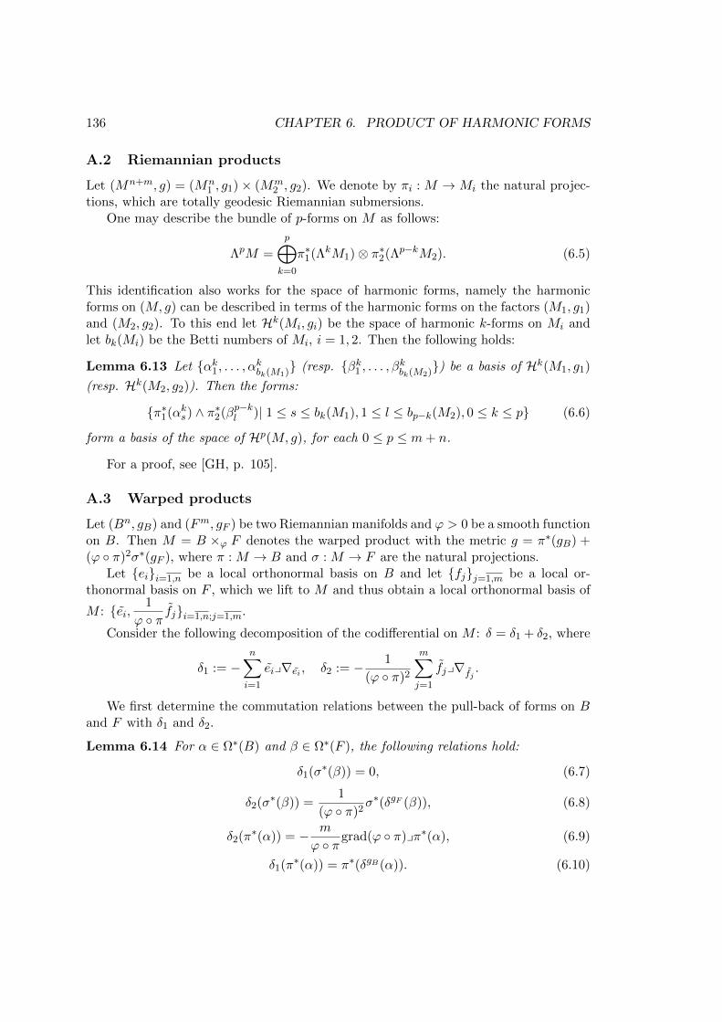
136 CHAPTER 6. PRODUCT OF HARMONIC FORMS
A.2 Riemannian products
Let (Mn+m, g) = (Mn1 , g1)× (Mm
2 , g2). We denote by πi : M →Mi the natural projec-tions, which are totally geodesic Riemannian submersions.
One may describe the bundle of p-forms on M as follows:
ΛpM =
p⊕k=0
π∗1(ΛkM1)⊗ π∗2(Λp−kM2). (6.5)
This identification also works for the space of harmonic forms, namely the harmonicforms on (M, g) can be described in terms of the harmonic forms on the factors (M1, g1)and (M2, g2). To this end let Hk(Mi, gi) be the space of harmonic k-forms on Mi andlet bk(Mi) be the Betti numbers of Mi, i = 1, 2. Then the following holds:
Lemma 6.13 Let αk1 , . . . , αkbk(M1) (resp. βk1 , . . . , βkbk(M2)) be a basis of Hk(M1, g1)
(resp. Hk(M2, g2)). Then the forms:
π∗1(αks) ∧ π∗2(βp−kl )| 1 ≤ s ≤ bk(M1), 1 ≤ l ≤ bp−k(M2), 0 ≤ k ≤ p (6.6)
form a basis of the space of Hp(M, g), for each 0 ≤ p ≤ m+ n.
For a proof, see [GH, p. 105].
A.3 Warped products
Let (Bn, gB) and (Fm, gF ) be two Riemannian manifolds and ϕ > 0 be a smooth functionon B. Then M = B ×ϕ F denotes the warped product with the metric g = π∗(gB) +(ϕ π)2σ∗(gF ), where π : M → B and σ : M → F are the natural projections.
Let eii=1,n be a local orthonormal basis on B and let fjj=1,m be a local or-thonormal basis on F , which we lift to M and thus obtain a local orthonormal basis of
M : ei,1
ϕ πfji=1,n;j=1,m.
Consider the following decomposition of the codifferential on M : δ = δ1 + δ2, where
δ1 := −n∑i=1
eiy∇ei , δ2 := − 1
(ϕ π)2
m∑j=1
fjy∇fj .
We first determine the commutation relations between the pull-back of forms on Band F with δ1 and δ2.
Lemma 6.14 For α ∈ Ω∗(B) and β ∈ Ω∗(F ), the following relations hold:
δ1(σ∗(β)) = 0, (6.7)
δ2(σ∗(β)) =1
(ϕ π)2σ∗(δgF (β)), (6.8)
δ2(π∗(α)) = − m
ϕ πgrad(ϕ π)yπ∗(α), (6.9)
δ1(π∗(α)) = π∗(δgB (α)). (6.10)
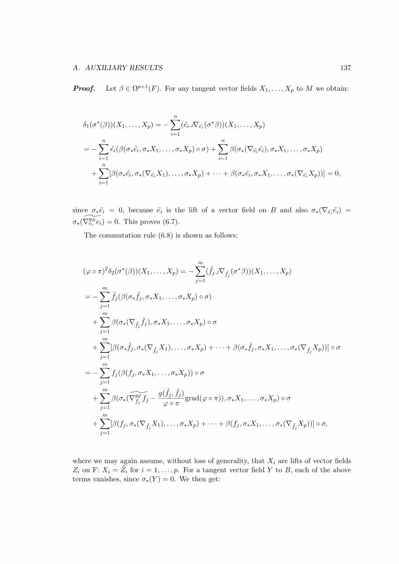
A. AUXILIARY RESULTS 137
Proof. Let β ∈ Ωp+1(F ). For any tangent vector fields X1, . . . , Xp to M we obtain:
δ1(σ∗(β))(X1, . . . , Xp) = −n∑i=1
(eiy∇ei(σ∗β))(X1, . . . , Xp)
=−n∑i=1
ei(β(σ∗ei, σ∗X1, . . . , σ∗Xp) σ) +
n∑i=1
β(σ∗(∇ei ei), σ∗X1, . . . , σ∗Xp)
+
n∑i=1
[β(σ∗ei, σ∗(∇eiX1), . . . , σ∗Xp) + · · ·+ β(σ∗ei, σ∗X1, . . . , σ∗(∇eiXp))] = 0,
since σ∗ei = 0, because ei is the lift of a vector field on B and also σ∗(∇ei ei) =
σ∗(∇gBei ei) = 0. This proves (6.7).
The commutation rule (6.8) is shown as follows:
(ϕ π)2δ2(σ∗(β))(X1, . . . , Xp) = −m∑j=1
(fjy∇fj (σ∗β))(X1, . . . , Xp)
=−m∑j=1
fj(β(σ∗fj , σ∗X1, . . . , σ∗Xp) σ)
+
m∑j=1
β(σ∗(∇fj fj), σ∗X1, . . . , σ∗Xp) σ
+
m∑j=1
[β(σ∗fj , σ∗(∇fjX1), . . . , σ∗Xp) + · · ·+ β(σ∗fj , σ∗X1, . . . , σ∗(∇fjXp))] σ
=−m∑j=1
fj(β(fj , σ∗X1, . . . , σ∗Xp)) σ
+m∑j=1
β(σ∗(∇gFfj fj −g(fj , fj)
ϕ πgrad(ϕ π)), σ∗X1, . . . , σ∗Xp) σ
+m∑j=1
[β(fj , σ∗(∇fjX1), . . . , σ∗Xp) + · · ·+ β(fj , σ∗X1, . . . , σ∗(∇fjXp))] σ,
where we may again assume, without loss of generality, that Xi are lifts of vector fieldsZi on F: Xi = Zi for i = 1, . . . , p. For a tangent vector field Y to B, each of the aboveterms vanishes, since σ∗(Y ) = 0. We then get:

138 CHAPTER 6. PRODUCT OF HARMONIC FORMS
(ϕ π)2δ2(σ∗(β))(X1, . . . , Xp) =
=−m∑j=1
fj(β(fj , Z1, . . . , Zp)) σ +m∑j=1
β(∇gFfj fj , Z1, . . . , Zp) σ
+
m∑j=1
[β(fj ,∇gFfj Z1, . . . , σ∗Xp) + · · ·+ β(fj , Z1, . . . ,∇gFfj Zp)] σ
=σ∗(δgF (β))(X1, . . . , Xp),
thus proving (6.8).The relations (6.9) and (6.10) can be obtained by similar computations, which we
omit here.
Acknowledgement. We thank D. Kotschick and P.-A. Nagy for very useful commentson the first draft of this note and S. Papadima for a discussion about topological formal-ity. We are also grateful to the referee for his suggestions which improved the structureof the paper and its presentation.
Bibliography
[B] F.A. Belgun, On the metric structure of non-Kahler complex surfaces, Math. Ann.317 (2000), 1–40.
[DO] S. Dragomir and L. Ornea, Locally conformal Kahler geometry, Progress in Math.155, Birkhauser, Boston, Basel, 1998.
[GH] Ph. Griffiths, J. Harris, Principles of algebraic geometry, Pure and Applied Math-ematics, Wiley-Interscience [John Wiley & Sons], New York, 1978.
[GN] J.-F. Grosjean, P.-A. Nagy, On the cohomology algebra of some classes of geomet-rically formal manifolds, Proc. Lond. Math. Soc. 98 (2009), 607–630.
[K] D. Kotschick, On products of harmonic forms, Duke Math. J. 107, (2001), 521–531.
[KT1] D. Kotschick, S. Terzic, On formality of generalized symmetric spaces, Math.Proc. Cambridge Philos. Soc. 134 (2003), 491–505.
[KT2] D. Kotschick, S. Terzic, Geometric formality of homogeneous spaces and of biquo-tients, arXiv:0901.2267, Pacific J. Math. (to appear).
[N] P.-A. Nagy, On length and product of harmonic forms in Kahler geometry, Math.Z. 254, 199–218.
[NV] P.-A. Nagy, C. Vernicos, The length of harmonic forms on a compact Riemannianmanifold, Trans. Amer. Math. Soc. 356 (2004), 2501–2513.
[OV1] L. Ornea, M. Verbitsky, Structure theorem for compact Vaisman manifolds, Math.Res. Lett. 10 (2003), 799–805.
[OV2] L. Ornea, M. Verbitsky, Topology of locally conformal Kahler manifolds withpotential, Int. Math. Res. Notices, 4 (2010), 117–126.
[PS] S. Papadima, A. Suciu, Geometric and algebraic aspects of 1-formality, Bull. Math.Soc. Sci. Math. Roumanie 52(100) (2009), 355–375.
[S] D. Sullivan, Infinitesimal computations in topology, Inst. Hautes Etudes Sci. Publ.Math. 47 (1977), 269–331.
139

140 BIBLIOGRAPHY
[T] Ph. Tondeur, Foliations on Riemannian Manifolds, Springer-Verlag, New York,1988.
[V] I. Vaisman, Generalized Hopf manifolds, Geom. Dedicata 13 (1982), 231–255.
[Ve] I. Verbitsky, Theorems on the vanishing of cohomology for locally conformallyhyper-Kahler manifolds, (Russian) Tr. Mat. Inst. Steklova 246 (2004), Algebr.Geom. Metody, Svyazi i Prilozh., 64–91; translation in Proc. Steklov Inst. Math.246 (2004), 54–78.


![Sub-Riemannian geometry, Hamiltonian dynamics, micro ... · Sub-Riemannian (SR) geometry in the framework of geometric optimal control was rst explored in the seminal article [17]](https://img.pdfslide.us/doc/110x75/5f4e7dcbb6f9633f2c3be174/sub-riemannian-geometry-hamiltonian-dynamics-micro-sub-riemannian-sr-geometry.jpg)
![Geometric Constructions and Structures Associated with Twistor … · 2020. 9. 2. · Moreover, [Sem01] discusses global properties of con-formal Killing forms on Riemannian manifolds](https://img.pdfslide.us/doc/110x75/60d87e8dfdcb706f1270ef79/geometric-constructions-and-structures-associated-with-twistor-2020-9-2-moreover.jpg)