SPE-KSA-8662-MS

Understanding the True Stimulated Reservoir Volume in Shale Reservoirs Maaruf Hussain, Bilal Saad, Ardiansyah Negara, Baker Hughes, Shuyu Sun, King Abdullah University of Science & Technology

Copyright 2017, Society of Petroleum Engineers This paper was prepared for presentation at the SPE Kingdom of Saudi Arabia Annual Technical Symposium and Exhibition held in Dammam, Saudi Arabia, 24–27 April 2017. This paper was selected for presentation by an SPE program committee following review of information contained in an abstract submitted by the author(s). Contents of the paper have not been reviewed by the Society of Petroleum Engineers and are subject to correction by the author(s). The material does not necessarily reflect any position of the Society of Petroleum Engineers, its officers, or members. Electronic reproduction, distribution, or storage of any part of this paper without the written consent of the Society of Petroleum Engineers is prohibited. Permission to reproduce in print is restricted to an abstract of not more than 300 words; illustrations may not be copied. The abstract must contain conspicuous acknowledgment of SPE copyright.

Abstract Successful exploitation of shale reservoirs largely depends on the effectiveness of hydraulic fracturing stimulation program. Favorable results have been attributed to intersection and reactivation of pre-existing fractures by hydraulically-induced fractures that connect the wellbore to a larger fracture surface area within the reservoir rock volume. Thus, accurate estimation of the stimulated reservoir volume (SRV) becomes critical for the reservoir performance simulation and production analysis. Micro-seismic events (MS) have been commonly used as a proxy to map out the SRV geometry, which could be erroneous because not all MS events are related to hydraulic fracture propagation. The case studies discussed here utilized a fully 3-D simulation approach to estimate the SRV. The simulation approach presented in this paper takes into account the real-time changes in the reservoir’s geomechanics as a function of fluid pressures. It consists of four separate coupled modules: geomechanics, hydrodynamics, a geomechanical joint model for interfacial resolution, and an adaptive re-meshing. Reservoir stress condition, rock mechanical properties, and injected fluid pressure dictate how fracture elements could open or slide. Critical stress intensity factor was used as a fracture criterion governing the generation of new fractures or propagation of existing fractures and their directions. Simulations were run on a Cray XC-40 HPC system. The results proved the approach of using MS data as a proxy for SRV to be significantly flawed. Many of the observed stimulated natural fractures were stress related and very few that were closer to the injection field were connected. The situation is worsened in a highly laminated shale reservoir as the hydraulic fracture propagation is significantly hampered. High contrast in the in-situ stresses related strike-slip developed thereby shortens the extent of SRV. However, far field natural fractures that were not connected to hydraulic fracture were observed being stimulated. These results show the beginning of new understanding into the physical mechanisms responsible for greater disparity in stimulation results within the same shale reservoir and hence the SRV. Using the appropriate methodology, stimulation design can be controlled to optimize the responses of in-situ stresses and reservoir rock itself. Introduction Ultralow-permeability and tiny porosity of shale reservoirs require a stimulation technique to extract hydrocarbon so called hydraulic fracturing. Hydraulic fracturing is conducted by pumping fluid into a reservoir at high pressure to create artificial fractures so that the hydrocarbon could flow easily to the

2 SPE-KSA-123-MS

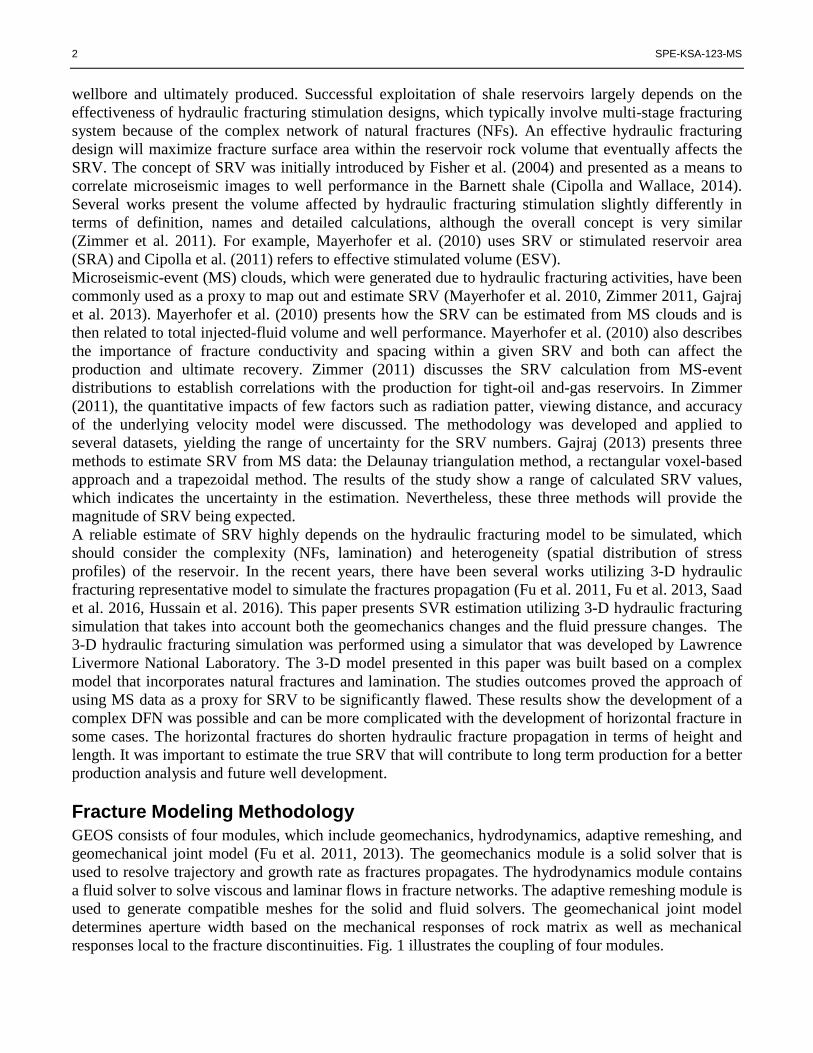
wellbore and ultimately produced. Successful exploitation of shale reservoirs largely depends on the effectiveness of hydraulic fracturing stimulation designs, which typically involve multi-stage fracturing system because of the complex network of natural fractures (NFs). An effective hydraulic fracturing design will maximize fracture surface area within the reservoir rock volume that eventually affects the SRV. The concept of SRV was initially introduced by Fisher et al. (2004) and presented as a means to correlate microseismic images to well performance in the Barnett shale (Cipolla and Wallace, 2014). Several works present the volume affected by hydraulic fracturing stimulation slightly differently in terms of definition, names and detailed calculations, although the overall concept is very similar (Zimmer et al. 2011). For example, Mayerhofer et al. (2010) uses SRV or stimulated reservoir area (SRA) and Cipolla et al. (2011) refers to effective stimulated volume (ESV). Microseismic-event (MS) clouds, which were generated due to hydraulic fracturing activities, have been commonly used as a proxy to map out and estimate SRV (Mayerhofer et al. 2010, Zimmer 2011, Gajraj et al. 2013). Mayerhofer et al. (2010) presents how the SRV can be estimated from MS clouds and is then related to total injected-fluid volume and well performance. Mayerhofer et al. (2010) also describes the importance of fracture conductivity and spacing within a given SRV and both can affect the production and ultimate recovery. Zimmer (2011) discusses the SRV calculation from MS-event distributions to establish correlations with the production for tight-oil and-gas reservoirs. In Zimmer (2011), the quantitative impacts of few factors such as radiation patter, viewing distance, and accuracy of the underlying velocity model were discussed. The methodology was developed and applied to several datasets, yielding the range of uncertainty for the SRV numbers. Gajraj (2013) presents three methods to estimate SRV from MS data: the Delaunay triangulation method, a rectangular voxel-based approach and a trapezoidal method. The results of the study show a range of calculated SRV values, which indicates the uncertainty in the estimation. Nevertheless, these three methods will provide the magnitude of SRV being expected. A reliable estimate of SRV highly depends on the hydraulic fracturing model to be simulated, which should consider the complexity (NFs, lamination) and heterogeneity (spatial distribution of stress profiles) of the reservoir. In the recent years, there have been several works utilizing 3-D hydraulic fracturing representative model to simulate the fractures propagation (Fu et al. 2011, Fu et al. 2013, Saad et al. 2016, Hussain et al. 2016). This paper presents SVR estimation utilizing 3-D hydraulic fracturing simulation that takes into account both the geomechanics changes and the fluid pressure changes. The 3-D hydraulic fracturing simulation was performed using a simulator that was developed by Lawrence Livermore National Laboratory. The 3-D model presented in this paper was built based on a complex model that incorporates natural fractures and lamination. The studies outcomes proved the approach of using MS data as a proxy for SRV to be significantly flawed. These results show the development of a complex DFN was possible and can be more complicated with the development of horizontal fracture in some cases. The horizontal fractures do shorten hydraulic fracture propagation in terms of height and length. It was important to estimate the true SRV that will contribute to long term production for a better production analysis and future well development. Fracture Modeling Methodology GEOS consists of four modules, which include geomechanics, hydrodynamics, adaptive remeshing, and geomechanical joint model (Fu et al. 2011, 2013). The geomechanics module is a solid solver that is used to resolve trajectory and growth rate as fractures propagates. The hydrodynamics module contains a fluid solver to solve viscous and laminar flows in fracture networks. The adaptive remeshing module is used to generate compatible meshes for the solid and fluid solvers. The geomechanical joint model determines aperture width based on the mechanical responses of rock matrix as well as mechanical responses local to the fracture discontinuities. Fig. 1 illustrates the coupling of four modules.

SPE-KSA-123-MS 3

Fig. 1. Four modules used in GEOS hydraulic fracturing simulator and their coupling (redrawn from Fu et al. 2011).

Solid Solver

The solid solver implements a conventional explicitly integrated finite element module, which uses linear-strain triangle (Veubeke triangle). The solver assumes linear elasticity and small deformations for the intact material response. A central-difference explicit time-integration scheme was used in this solver, where the dynamic responses were solved on a nodal basis as follows (Fu et al. 2013):

�̈�𝐮𝑖𝑖(𝑡𝑡) =𝐅𝐅𝑖𝑖(𝑡𝑡) − 𝐅𝐅𝑖𝑖𝐶𝐶(𝑡𝑡)

𝑚𝑚𝑖𝑖 (1)

�̇�𝐮𝑖𝑖 �𝑡𝑡 +∆𝑡𝑡𝑠𝑠2� − �̇�𝐮𝑖𝑖 �𝑡𝑡 −

∆𝑡𝑡𝑠𝑠2� = �̈�𝐮𝑖𝑖(𝑡𝑡)∆𝑡𝑡𝑠𝑠 (2)

𝐮𝐮𝑖𝑖(𝑡𝑡 + ∆𝑡𝑡𝑠𝑠) = 𝐮𝐮𝑖𝑖(𝑡𝑡) + �̇�𝐮𝑖𝑖 �𝑡𝑡 +∆𝑡𝑡𝑠𝑠2� ∆𝑡𝑡𝑠𝑠 (3)

where 𝐅𝐅𝑖𝑖 is the nodal force vector acting on node 𝑖𝑖 at each time step, 𝐅𝐅𝑖𝑖𝐶𝐶 is the nodal damping force, and 𝐮𝐮𝑖𝑖 , �̇�𝐮𝑖𝑖, and �̈�𝐮𝑖𝑖 are the nodal displacement, velocity, and acceleration vectors, respectively.

Fluid Solver The fluid solver assumes laminar flow between two parallel plates to represent the fluid flow in open rock fractures and the governing equations are described as follows (Fu et al. 2013):

𝜕𝜕𝜕𝜕𝜕𝜕𝜕𝜕

+𝜕𝜕𝜕𝜕𝜕𝜕𝑡𝑡

= 0 (4)

4 SPE-KSA-123-MS

𝑘𝑘𝜕𝜕𝜕𝜕𝜕𝜕𝜕𝜕

= −𝜕𝜕 (5)

𝑘𝑘 =𝜕𝜕3

12𝜇𝜇 (6)

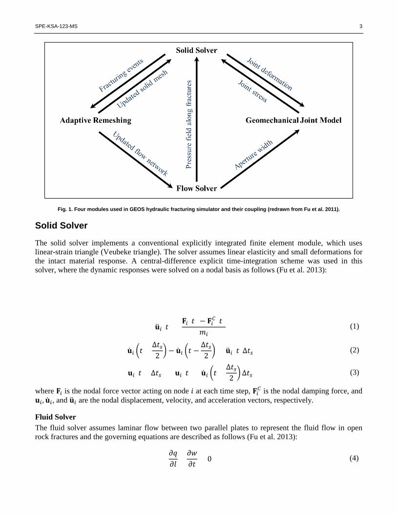
where 𝜕𝜕 is the length along the fracture, 𝜕𝜕 is the aperture size, 𝜕𝜕 is the flow rate in the fracture at a given cross-section, 𝑘𝑘 is the permeability of the fracture, 𝜕𝜕 is the fluid pressure inside the fracture, 𝜇𝜇 is the dynamic viscosity of the fluid, and 𝑡𝑡 is time. The critical time step for the flow solver is calculated as follows:

∆𝑡𝑡 =6𝜇𝜇𝐾𝐾�𝐿𝐿𝑖𝑖𝑖𝑖𝜕𝜕𝑖𝑖𝑖𝑖

�2

(7)

where 𝐿𝐿𝑖𝑖𝑖𝑖 is the distance between the centers of two adjacent flow cells 𝑖𝑖, and 𝑗𝑗; 𝜕𝜕𝑖𝑖𝑖𝑖 is their homogenized average aperture size; and 𝐾𝐾 is the fluid bulk modulus. Eqs. (4)-(6) are solved with a 2-D finite volume method formulated based on a three-dimensional approach (Johnson and Morris 2009). In this study, the discrete fracture network (DFN) and lamination in considered in the numerical models. Since there were constraints with limited data, a structured DFN realization was generated that consists of deterministic wellbore image-based model to develop a simple stochastic model of fractures between and around wellbores based on the conceptual models for fracture orientation, spatial distribution, and the intensity-size scaling discussed above. Laminations (Lams) are horizontal weak planes in the reservoirs and were incorporated into the models as horizontal natural fractures. Furthermore, the results take into account the wellbore hydraulics in the model in order to investigate the hydraulic fracture propagation behavior in the presence of perforation and wellbore friction. The perforation friction is given by (Izadi et al. 2015)

𝑄𝑄𝑡𝑡𝑡𝑡𝑡𝑡𝑡𝑡𝑡𝑡 = �𝑄𝑄𝑖𝑖

𝑛𝑛

𝑖𝑖=1

(8)

𝜕𝜕𝑡𝑡 = 𝜕𝜕𝑐𝑐,𝑖𝑖 + ∆𝜕𝜕𝑛𝑛,𝑖𝑖 + ∆𝜕𝜕𝑝𝑝𝑝𝑝,𝑖𝑖(𝑄𝑄𝑖𝑖) + ∆𝜕𝜕𝑐𝑐𝑝𝑝,𝑖𝑖(𝑄𝑄𝑖𝑖) (9)

where 𝑄𝑄𝑡𝑡𝑡𝑡𝑡𝑡𝑡𝑡𝑡𝑡 is the total flow rate, 𝜕𝜕𝑡𝑡 is the reference pressure at bottomhole, 𝜕𝜕𝑐𝑐,𝑖𝑖 is the closure pressure of each frac, ∆𝜕𝜕𝑛𝑛,𝑖𝑖 is the net pressure of each frac, and ∆𝜕𝜕𝑝𝑝𝑝𝑝,𝑖𝑖(𝑄𝑄𝑖𝑖) is the perforation friction of each frac, and ∆𝜕𝜕𝑐𝑐𝑝𝑝,𝑖𝑖(𝑄𝑄𝑖𝑖) is the casing friction.The perforation friction, ∆𝜕𝜕𝑝𝑝𝑝𝑝,𝑖𝑖(𝑄𝑄𝑖𝑖), is calculated by

∆𝜕𝜕𝑝𝑝𝑝𝑝,𝑖𝑖(𝑄𝑄𝑖𝑖) =0.2369𝜌𝜌𝑄𝑄𝑖𝑖2

𝑑𝑑4𝐶𝐶𝑑𝑑2𝑁𝑁2 (10)

where 𝝆𝝆 is the fluid density, 𝑸𝑸𝒊𝒊 is the total flow rate, 𝑵𝑵 is the number of perforations, 𝒅𝒅 is the perforation diameter, and 𝑪𝑪𝒅𝒅 is the discharge coefficient, which captures perforation tunnel effects.

Model Setup

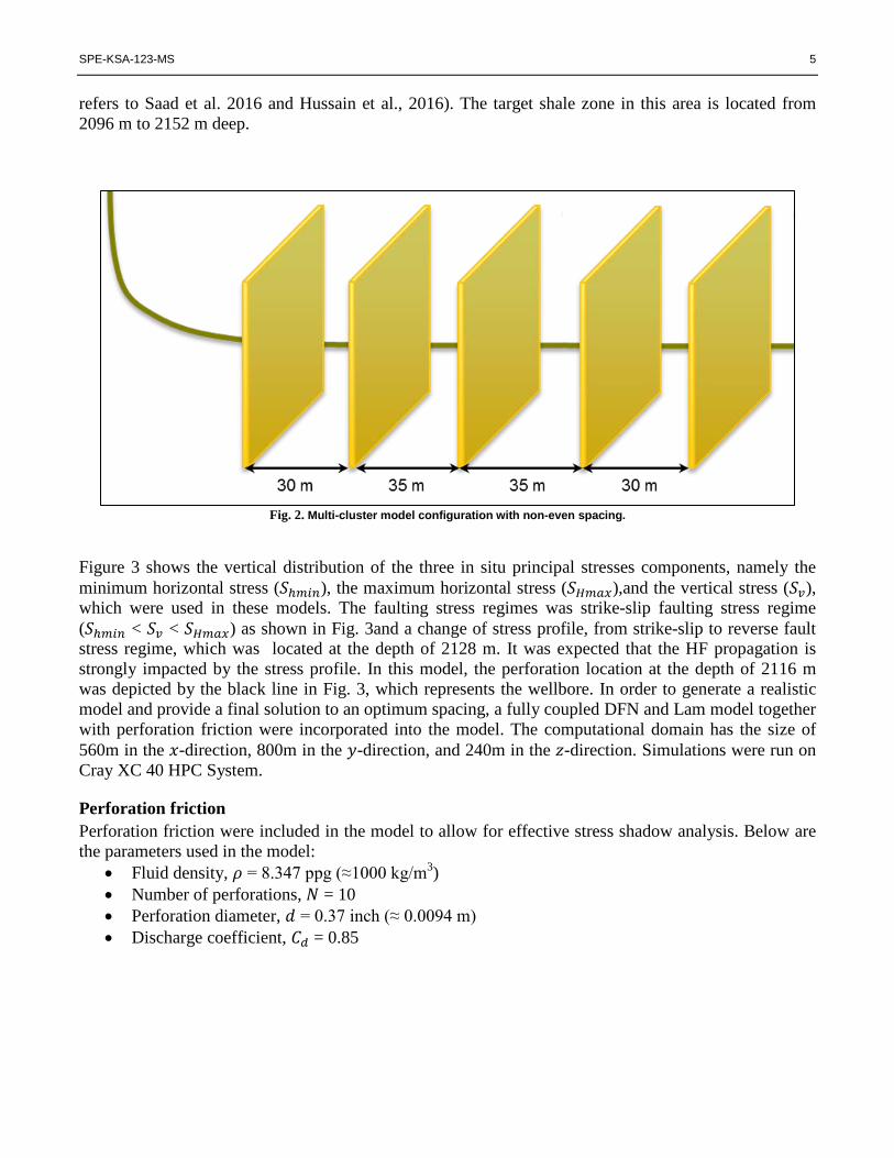
The setup considers a multi-cluster model configuration with non-even spacing configuration between the fractures. The spacing configuration was 30/35/35/30 m (Fig. 2). The fluid pumping rate was 30 BPM and the fluid viscosity was 40 centipoise (cP). The simulation time was 3600s, which represents one hour of hydraulic fracturing job in the field. The stress profiles of the Western Canada Sedimentary Basin (Bell et al. 1994) were used in this study. In general, the model setup of the study in this paper

SPE-KSA-123-MS 5

refers to Saad et al. 2016 and Hussain et al., 2016). The target shale zone in this area is located from 2096 m to 2152 m deep.

Fig. 2. Multi-cluster model configuration with non-even spacing.

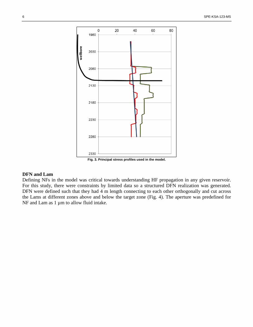
Figure 3 shows the vertical distribution of the three in situ principal stresses components, namely the minimum horizontal stress (𝑆𝑆ℎ𝑚𝑚𝑖𝑖𝑛𝑛), the maximum horizontal stress (𝑆𝑆𝐻𝐻𝑚𝑚𝑡𝑡𝐻𝐻),and the vertical stress (𝑆𝑆𝑣𝑣), which were used in these models. The faulting stress regimes was strike-slip faulting stress regime (𝑆𝑆ℎ𝑚𝑚𝑖𝑖𝑛𝑛 < 𝑆𝑆𝑣𝑣 < 𝑆𝑆𝐻𝐻𝑚𝑚𝑡𝑡𝐻𝐻) as shown in Fig. 3and a change of stress profile, from strike-slip to reverse fault stress regime, which was located at the depth of 2128 m. It was expected that the HF propagation is strongly impacted by the stress profile. In this model, the perforation location at the depth of 2116 m was depicted by the black line in Fig. 3, which represents the wellbore. In order to generate a realistic model and provide a final solution to an optimum spacing, a fully coupled DFN and Lam model together with perforation friction were incorporated into the model. The computational domain has the size of 560m in the 𝑥𝑥-direction, 800m in the 𝑦𝑦-direction, and 240m in the 𝑧𝑧-direction. Simulations were run on Cray XC 40 HPC System.

Perforation friction Perforation friction were included in the model to allow for effective stress shadow analysis. Below are the parameters used in the model:

• Fluid density, 𝜌𝜌 = 8.347 ppg (≈1000 kg/m3) • Number of perforations, 𝑁𝑁 = 10 • Perforation diameter, 𝑑𝑑 = 0.37 inch (≈ 0.0094 m) • Discharge coefficient, 𝐶𝐶𝑑𝑑 = 0.85

6 SPE-KSA-123-MS

Fig. 3. Principal stress profiles used in the model.

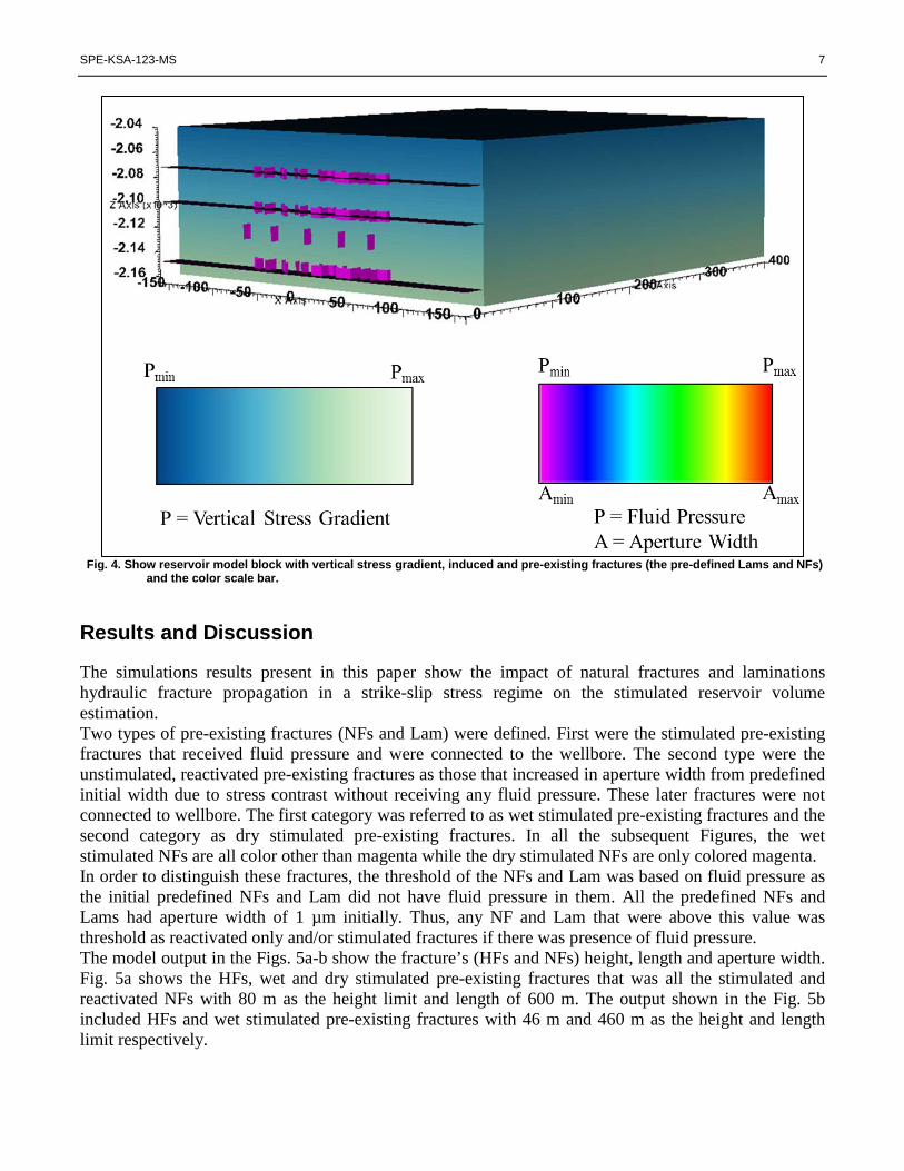
DFN and Lam Defining NFs in the model was critical towards understanding HF propagation in any given reservoir. For this study, there were constraints by limited data so a structured DFN realization was generated. DFN were defined such that they had 4 m length connecting to each other orthogonally and cut across the Lams at different zones above and below the target zone (Fig. 4). The aperture was predefined for NF and Lam as 1 µm to allow fluid intake.

SPE-KSA-123-MS 7

Fig. 4. Show reservoir model block with vertical stress gradient, induced and pre-existing fractures (the pre-defined Lams and NFs)

and the color scale bar.

Results and Discussion

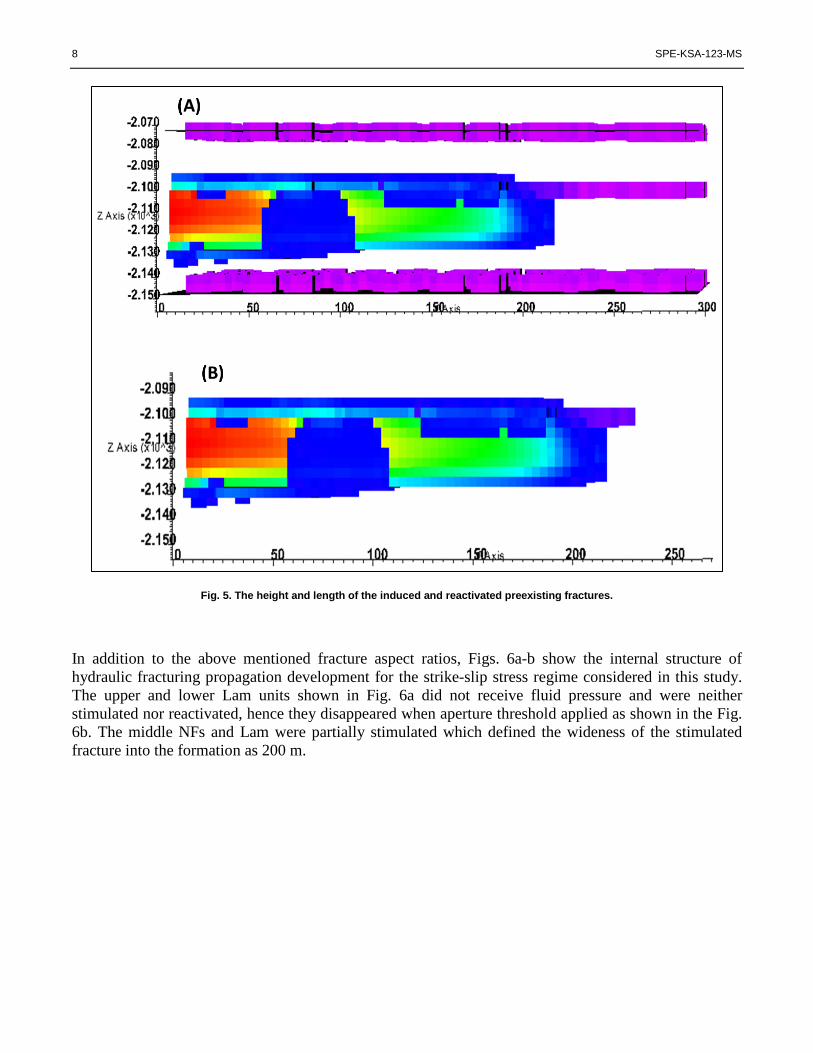
The simulations results present in this paper show the impact of natural fractures and laminations hydraulic fracture propagation in a strike-slip stress regime on the stimulated reservoir volume estimation. Two types of pre-existing fractures (NFs and Lam) were defined. First were the stimulated pre-existing fractures that received fluid pressure and were connected to the wellbore. The second type were the unstimulated, reactivated pre-existing fractures as those that increased in aperture width from predefined initial width due to stress contrast without receiving any fluid pressure. These later fractures were not connected to wellbore. The first category was referred to as wet stimulated pre-existing fractures and the second category as dry stimulated pre-existing fractures. In all the subsequent Figures, the wet stimulated NFs are all color other than magenta while the dry stimulated NFs are only colored magenta. In order to distinguish these fractures, the threshold of the NFs and Lam was based on fluid pressure as the initial predefined NFs and Lam did not have fluid pressure in them. All the predefined NFs and Lams had aperture width of 1 µm initially. Thus, any NF and Lam that were above this value was threshold as reactivated only and/or stimulated fractures if there was presence of fluid pressure. The model output in the Figs. 5a-b show the fracture’s (HFs and NFs) height, length and aperture width. Fig. 5a shows the HFs, wet and dry stimulated pre-existing fractures that was all the stimulated and reactivated NFs with 80 m as the height limit and length of 600 m. The output shown in the Fig. 5b included HFs and wet stimulated pre-existing fractures with 46 m and 460 m as the height and length limit respectively.

8 SPE-KSA-123-MS

Fig. 5. The height and length of the induced and reactivated preexisting fractures.

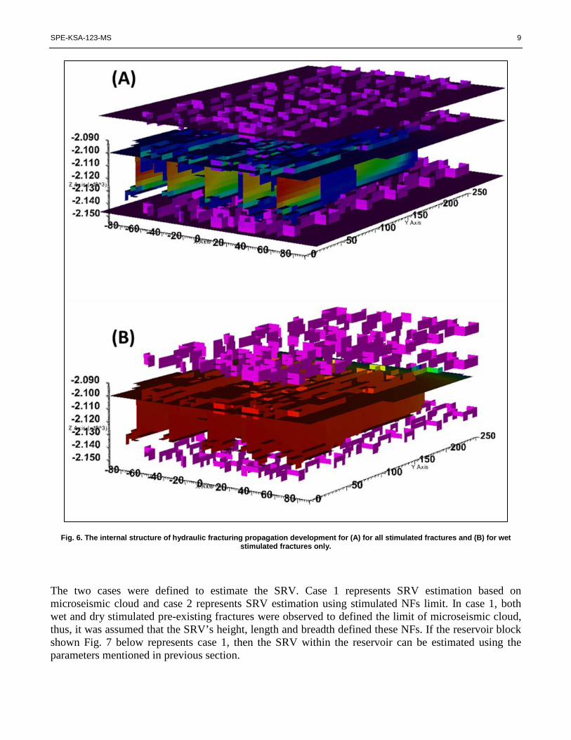
In addition to the above mentioned fracture aspect ratios, Figs. 6a-b show the internal structure of hydraulic fracturing propagation development for the strike-slip stress regime considered in this study. The upper and lower Lam units shown in Fig. 6a did not receive fluid pressure and were neither stimulated nor reactivated, hence they disappeared when aperture threshold applied as shown in the Fig. 6b. The middle NFs and Lam were partially stimulated which defined the wideness of the stimulated fracture into the formation as 200 m.

SPE-KSA-123-MS 9

Fig. 6. The internal structure of hydraulic fracturing propagation development for (A) for all stimulated fractures and (B) for wet

stimulated fractures only.

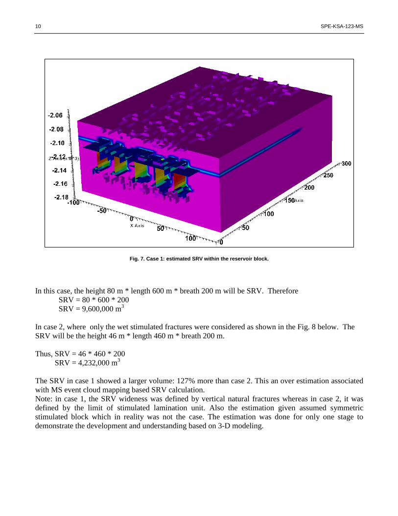
The two cases were defined to estimate the SRV. Case 1 represents SRV estimation based on microseismic cloud and case 2 represents SRV estimation using stimulated NFs limit. In case 1, both wet and dry stimulated pre-existing fractures were observed to defined the limit of microseismic cloud, thus, it was assumed that the SRV’s height, length and breadth defined these NFs. If the reservoir block shown Fig. 7 below represents case 1, then the SRV within the reservoir can be estimated using the parameters mentioned in previous section.

10 SPE-KSA-123-MS

Fig. 7. Case 1: estimated SRV within the reservoir block.

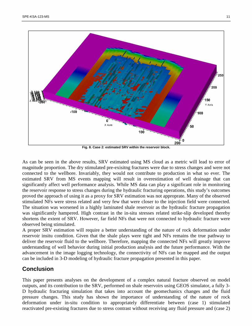
In this case, the height 80 m * length 600 m * breath 200 m will be SRV. Therefore SRV = 80 * 600 * 200 SRV = 9,600,000 m3 In case 2, where only the wet stimulated fractures were considered as shown in the Fig. 8 below. The SRV will be the height 46 m * length 460 m * breath 200 m. Thus, SRV = 46 * 460 * 200 SRV = 4,232,000 m3 The SRV in case 1 showed a larger volume: 127% more than case 2. This an over estimation associated with MS event cloud mapping based SRV calculation. Note: in case 1, the SRV wideness was defined by vertical natural fractures whereas in case 2, it was defined by the limit of stimulated lamination unit. Also the estimation given assumed symmetric stimulated block which in reality was not the case. The estimation was done for only one stage to demonstrate the development and understanding based on 3-D modeling.

SPE-KSA-123-MS 11

Fig. 8. Case 2: estimated SRV within the reservoir block.

As can be seen in the above results, SRV estimated using MS cloud as a metric will lead to error of magnitude proportion. The dry stimulated pre-exisitng fractures were due to stress changes and were not connected to the wellbore. Invariably, they would not contribute to production in what so ever. The estimated SRV from MS events mapping will result in overestimation of well drainage that can significantly affect well performance analysis. While MS data can play a significant role in monitoring the reservoir response to stress changes during the hydraulic fracturing operations, this study’s outcomes proved the approach of using it as a proxy for SRV estimation was not approprate. Many of the observed stimulated NFs were stress related and very few that were closer to the injection field were connected. The situation was worsened in a highly laminated shale reservoir as the hydraulic fracture propagation was significantly hampered. High contrast in the in-situ stresses related strike-slip developed thereby shortens the extent of SRV. However, far field NFs that were not connected to hydraulic fracture were observed being stimulated. A proper SRV estimation will require a better understanding of the nature of rock deformation under reservoir insitu condition. Given that the shale plays were tight and NFs remains the true pathway to deliver the reservoir fluid to the wellbore. Therefore, mapping the connected NFs will greatly improve understanding of well behavior during initial production analysis and the future performance. With the advancement in the image logging technology, the connectivity of NFs can be mapped and the output can be included in 3-D modeling of hydraulic fracture propagation presented in this paper.

Conclusion

This paper presents analyses on the development of a complex natural fracture observed on model outputs, and its contribution to the SRV, performed on shale reservoirs using GEOS simulator, a fully 3-D hydraulic fracturing simulation that takes into account the geomechanics changes and the fluid pressure changes. This study has shown the importance of understanding of the nature of rock deformation under in-situ condition to appropriately differentiate between (case 1) stimulated reactivated pre-existing fractures due to stress contrast without receiving any fluid pressure and (case 2)

12 SPE-KSA-123-MS

pre-existing fractures that received fluid pressure and were connected to the wellbore and unstimulated. Far field natural fractures that were not connected to hydraulic fracture were observed being stimulated and by calculating the SRV in the two cases, in the first case the SRV has shown larger volume 127% more than case 2. Through the calculations of accurately SVR, these results show the beginning of new understanding into the physical mechanisms responsible for greater disparity in stimulation results within the same shale reservoir and hence the SRV. Simulation were run on Cray XC 40 HPC system. These results demonstrated the beginning of new understanding into the physical mechanisms responsible for greater disparity in stimulation results within the same shale reservoir and hence the SRV. Using the appropriate methodology, stimulation design can be controlled to optimize the responses of in-situ stresses and reservoir rock itself.

Acknowledgements The authors thank the management of Baker Hughes for the permission to present this paper and to King Abdullah University of Science and Technology (KAUST) for providing access to Shaheen Cray XC-40 HPC system. References Bell, J.S., Price, P.R. and McLellan, P.J. 1994. In-Situ Stress in the Western Canada Sedimentary Basin. In: Geological Atlas of the

Western Canada Sedimentary Basin, G.D. Mossop and I. Shetsen (comp). Canadian Society of Petroleum Geologists and Alberta Research Council.

Cipolla, C., Maxwell, S., Mack, M. et al. 2011. A Practical Guide to Interpreting Microseismic Measurements. Presented at the SPE North American Unconventional Gas Conference and Exhibition held in The Woodlands, Texas, USA. 14-16 June. SPE-144067-MS. https://doi.org/10.2118/144067-MS.

Cipolla, C. and Wallace, J. 2014. Stimulated Reservoir Volume: A Missapplied Concept? Presented at the SPE Hydraulic Fracturing Technology Conference held in The Woodlands, Texas, USA, 4-6 February. SPE-168596-MS. https://doi.org/10.2118/168596-MS.

Fisher, M.K., Heinze, J.R., Harris, C.D. et al. 2004. Optimizing Horizontal Completion Techniques in the Barnett Shale Using Microseismic Fracture Mapping. Presented at the 2004 SPE Annual Technical Conference and Exhibition held in Houston, Texas, USA, 26-29 September. SPE-90051-MS. https://doi.org/10.2118/90051-MS.

Fu, P., Johnson, S.M., and Carrigan, C.R. 2011. Simulating Complex Fracture Systems in Geothermal Reservoirs Using an Explicitly Coupled Hydro-Geomechanical Model. Presented at the 45th US Rock Mechanics/Geomechanics Symposium held in San Fransisco, California, 26-29 June.

Fu, P., Johnson, S.M., and Carrigan, C.R. 2013. An Explicitly Coupled Hydro-Geomechanical Model for Simulating Hydraulic Fracturing in Arbitrary Discrete Fracture Networks. International Journal for Numerical and Analytical Methods in Geomechanics 37: 2278-2300.

Gajraj, A., Lin, A., Kiang, C. et al. 2013. SRV Estimation Using Hydraulic Fracture Microseismic Event Data. Presented at the 75th EAGE Conference and Exhibition incorporating SPE EUROPEC held in London, UK, 10-13 June. CSUG/SPE-148610-MS. https://doi.org/10.3997/2214-4609.20130556.

Hussain, M., Saad, B., Negara, A. et al. 2016. Hydraulic Fracture Propagation in Highly Laminated Shale Reservoir with Complex Natural Fracture Network – Case Study Using Higher-Accuracy, Full 3-D Simulation. Presented at the SPE Annual Technical Conference and Exhibition held in Dubai, UAE, 26-28 September. SPE-181530-MS. https://doi.org/10.2118/181530-MS.

Izada, G., Moos, D., Settgast, R. et al. 2015. Fully 3D Hydraulic Fracture Growth within Multi-stage Horizontal Wells. Presented at the International Congress on Rock Mechanics held in Montreal, Quebec, Canada.

Johnson, S.M. and Morris, J.P. Hydraulic Fracturing Mechanisms in Carbon Sequestration Applications. Presented at the 43rd US Rock Mechanics Symposium and the 4th US-Canada Rock Mechanics Symposium, Asheville, NC, 28 June-1 July.

Mayerhofer, M.J., Lolon, E.P., Warpinski, N.R. et al. 2010. What is Stimulated Reservoir Volume?. SPE Production and Operations 25(1): 89-98.

Saad, B., Negara, A., Hussain, M. et al. 2016. Enhancing Oil Recovery – Advanced Simulations for More Accurate Frac-Stages Placement. Presented at the SPE Kingdom of Saudi Arabia Annual Technical Symposium and Exhibition held in Dammam, Saudi Arabia, 25-28 April. SPE-182747-MS. https://doi.org/10.2118/182747-MS.

Zimmer, U. 2011. Calculating Stimulated Reservoir Volume (SRV) with Consideration of Uncertainties in Microseismic-Event Locations. Presented at the Canadian Unconventional Resources Conference held in Calgary, Alberta, Canada, 15-17 November. CSUG/SPE-148610-MS. https://doi.org/10.2118/148610-MS.