SPE-200527-MS

Evaluating the Effects of Acid Fracture Etching Patterns on ConductivityEstimation Using Machine Learning Techniques

Mahmoud Desouky and Murtada Saleh Aljawad, King Fahd University of Petroleum and Minerals; Hamed Alhoori,Northern Illinois University; Dhafer Al-Shehri, King Fahd University of Petroleum and Minerals

Copyright 2020, Society of Petroleum Engineers

This paper was prepared for presentation at the SPE Europec featured at 82nd EAGE Conference and Exhibition originally scheduled to be held in Amsterdam, TheNetherlands, 8 - 11 June 2020. Due to COVID-19 the physical event was postponed until 8 – 11 December 2020. The official proceedings were published online on8 June 2020.

This paper was selected for presentation by an SPE program committee following review of information contained in an abstract submitted by the author(s). Contentsof the paper have not been reviewed by the Society of Petroleum Engineers and are subject to correction by the author(s). The material does not necessarily reflectany position of the Society of Petroleum Engineers, its officers, or members. Electronic reproduction, distribution, or storage of any part of this paper without the writtenconsent of the Society of Petroleum Engineers is prohibited. Permission to reproduce in print is restricted to an abstract of not more than 300 words; illustrations maynot be copied. The abstract must contain conspicuous acknowledgment of SPE copyright.

AbstractThe successful design of an acid fracture job requires accurate prediction of fractured well productivity.Productivity estimation demands knowledge of both the acid penetration length and conductivitydistribution for the given reservoir. The literature includes several models developed to predict theconductivity of acid fractured rock. The most popular is empirical and based on measuring the conductivityof 25 acid fracture experiments. The present research provides empirical models utilizing machine learningtechniques and incorporating 97 experiments and 563 datapoints.

We conducted an extensive literature review to collect the published data on acid fracture experiments.The objective of such experiments is to measure conductivity at different formation closure stresses whileconsidering field conditions. We used several data preprocessing techniques to clean the data, fill in missingvalues, exclude outliers and failed experiments, and standardize the dataset. Regularization was employedto eliminate features that didn't contribute to accurate prediction. Feature engineering was used to constructnew features from our dataset. We began by measuring the correlations between features to better understandthe data. We then built various machine learning models to predict acid fracture conductivity.

It has been observed that developing one universal empirical correlation often results in significanterrors in conductivity estimation because different rock types result in different etching patterns that cannotbe explained by a single correlation. For instance, the channeling etching pattern is mostly observedin limestone formations, while a roughness pattern is seen in dolomite and chalk rock. Moreover, theconductivities of etching patterns formed in chalk, dolomite, and limestone formations behave differently.We built machine learning classification techniques to determine the most likely etching patterns (e.g.,channeling, roughness). A linear regression-based model was then developed as a baseline for comparisonwith other models generated through ridge regression. We evaluated the performances of our models usingwell-known metrics such as accuracy, precision, recall, mean squared error, and correlation coefficients. Wealso employed cross-validation to avoid over-fitting, finding that certain features were the most importantin predicting acid fracture conductivity.

2 SPE-200527-MS

Detailed empirical conductivity correlations and models were developed in this work for three carbonaterock types. Previously, a single empirical model has often been employed to estimate acid fractureconductivity or, at best, a model has been developed for a particular rock type. Most models have notconsidered the impact of etching patterns on conductivity, which was found to be significant in limestone.

IntroductionAcid fracturing is a well stimulation method applied to tight carbonate reservoirs. A hydraulic fracture iscreated when the treatment pressure exceeds the formation breakdown pressure. The formation stressesusually close the hydraulic fracture once pumping ceases. Prior to this cessation, fracture face asperities propthe fracture open against closure stress, providing a conductive path for reservoir fluids. Rock heterogeneityresults in uneven surfaces, improving fracture conductivity (Williams et al., 1979; Asadollahpour et al.,2018). Conductivity is defined as the ability of a fracture to deliver fluids; it decreases as the formationclosure stress increases. A successful acid fracture job produces sufficient durable conductivity.

Predicting acid fracture conductivity is essential to improving acid fracture design. Acid/rock dissolutionis a stochastic phenomenon that depends on a number of parameters. Thus, prediction of the resultingconductivity can be challenging. Different approaches have been taken to predict acid fracture conductivity,as summarized in Table 1. Empirical correlations based on experimental studies are convenient to applybecause their parameters are easy to obtain. Analytical correlations based on theoretical derivations arecomplicated and require sophisticated parameters. These parameters may demand experiments to tune themfor a regression analysis. Artificial intelligence models require accurate, consistent, and sizeable datasetsto be viable.

Table 1—Conductivity Correlations

Analytical Numerical Empirical Artificial Intelligence

Gangi, 1978 Deng-Mou et al., 2010 Nierode-Kruck, 1973 Akbari et al., 2017

Walsh, 1981 Kamali et al., 2015 Nasr-Eldin et al., 2006 Eliebid et al., 2018

Gong, 1997 Pournik, 2009 Motamedi-Ghahfarokhi et al., 2018

Nierode and Kruck (1973) suggested that among other parameters, the amount of rock dissolved can beused to determine acid fracture conductivity. Recent research has also shown that the pattern of rock removalhas a crucial effect on hydraulic fracture conductivity, even more so than the amount of dissolved rock(Pournik, 2008). For instance, conductivity is higher when the acid fracture treatment generates channelsinstead of rough surfaces, given that such channels withstand closure stress (van Domelen et al., 1994; Ruffetet al., 1998; Beg et al., 1998; Nieto et al., 2006; Melendez, 2007; Antelo, 2009; Cash, 2016; Kamali et al.,2016; Lu et al., 2017). The leak-off of acid into the formation matrix can also result in more heterogeneousfracture surfaces that boost conductivity when the rock's mechanical properties are unharmed (Beg et al.,1998).

Pournik (2008) categorized etching patterns of rock samples after acidization into five categories. Theroughness etching pattern occurs when acid etches the rock, leaving asperities distributed on the fracturesurface. The channeling etching pattern is characterized by a V-shape where the acid etches the middlemore than the edges. Cavity and turbulence etching patterns are similar in that pockets are formed by theacid etching. The uniform etching pattern occurs due to low reactivity of the rock with the acid or rockmineral homogeneity. In similar acid systems, contact time can influence the etching pattern. Also, acidconcentration, which changes along the fracture length, affects the amount of rock dissolved as well asthe etching pattern (Pournik et al., 2013). Roughness is more likely to be generated when smooth surfacesare being acidized, while acidization of rough surfaces deepens valleys and smoothens peaks (Al-Momin

SPE-200527-MS 3

et al., 2014). Pournik (2008) employed both theoretical and empirical methods to develop conductivitycorrelations for the roughness etching pattern, considering each rock type separately.

Few models account for the contribution of channels to conductivity, which provide higher conductivityat low stress and durable conductivity after fracture closure. Large channel dimensions make the floweasier and pressure drop lower. Deng and Mou (2012) captured their effect through numerical studies,enhancing conductivity prediction. They classified etching patterns into three categories: permeabilitydistribution dominant, mineralogy distribution dominant, and competing effect of permeability andmineralogy distributions. To apply their correlations, six parameters are needed: ideal fracture width, idealYoung's modulus, calcite fraction, horizontal and vertical correlation lengths, and standard deviation forpermeability distribution. Almomen (2013) showed that rough surface fractures generate conductivity anorder of magnitude higher than do smooth surface fractures at low closure stresses. Thus, ignoring suchfactors will yield simple models, but such models will be inaccurate and biased. We investigated the effectsof different features such as etching patterns on conductivity prediction.

Data Gathering and HandlingAn extensive literature review was conducted to collect published data on acid fracture experiments (Hill etal., 2007; Melendez, 2007; Pournik, 2009; Almomen, 2013; Nino, 2013; Cash, 2016; Jin et al., 2019). Thephysical properties, meanings, and units of different features are described in Table 2.

Table 2—Physical Meaning of Features

Feature Symbol Physical Meaning and Unit

Rock Type X1 Rocks etched by different acids

Acid Type X2 Acid systems used to etch rocks

Rock Surface X3 Initial rock surface before acid etching

Etching Pattern X4 Manner of rock surface behavior after acid etching

Temperature X5 Temperature of etching acid in °F

Injection Rate X6 Rate of pumping acid through API conductivity cell in liters per minute

Injection Time X7 Time for pumping acid through API conductivity cell in minutes

Acid Concentration X8 Concentration of etching acid pumped through API conductivity cell as a percentage

Stress X9 Applied stress by loading frame in psi

Conductivity Y Resultant rock conductivity under stress in md-ft

The objective of the acid fracture experiment was to measure conductivity at different formation closurestresses while mimicking field conditions (e.g., rock type, acid type, injection rate, treatment volume).The conditions were scaled down to represent the field conditions. The rock types and their initial surfaceconditions were tabulated, along with the treatment conditions (e.g., temperature, injection time). Next, theetching pattern and conductivity at each load stress were compiled to complete the dataset, as shown inTable 3 (Desouky, 2019). Therefore, the data gathered were consistent because the datapoints came fromthe same modified API RP-61 conductivity cell (Zou, 2006).

Table 3—Sample of Data Collected

X1 X2 X3 X4 X5 X6 X7 X8 X9 Y

Chalk GelledAcid Rough Channeling 175 1 30 15 3000 90

Chalk Straight Smooth Turbulence 175 1 5 15 100 2778

4 SPE-200527-MS

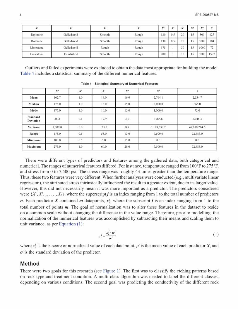
X1 X2 X3 X4 X5 X6 X7 X8 X9 Y

Dolomite GelledAcid Smooth Rough 130 0.5 20 15 500 127

Dolomite GelledAcid Smooth Rough 130 0.5 20 15 1000 104

Limestone GelledAcid Rough Rough 175 1 30 15 5000 72

Limestone Emulsified Smooth Rough 200 1 15 15 1000 1597

Outliers and failed experiments were excluded to obtain the data most appropriate for building the model.Table 4 includes a statistical summary of the different numerical features.

Table 4—Statistical Summary of Numerical Features

X5 X6 X7 X8 X9 Y

Mean 162.7 1.0 19.0 16.0 2,764.1 2,534.7

Median 175.0 1.0 15.0 15.0 3,000.0 366.0

Mode 175.0 1.0 10.0 15.0 1,000.0 72.0

StandardDeviation 36.2 0.1 12.9 3.0 1768.8 7,048.3

Variance 1,309.0 0.0 165.7 8.9 3,128,639.2 49,678,784.6

Range 175.0 0.5 55.0 13.0 7,500.0 72,483.0

Minimum 100.0 0.5 5.0 15.0 0.0 0.0

Maximum 275.0 1.0 60.0 28.0 7,500.0 72,483.0

There were different types of predictors and features among the gathered data, both categorical andnumerical. The ranges of numerical features differed. For instance, temperature ranged from 100°F to 275°F,and stress from 0 to 7,500 psi. The stress range was roughly 43 times greater than the temperature range.Thus, these two features were very different. When further analyses were conducted (e.g., multivariate linearregression), the attributed stress intrinsically influenced the result to a greater extent, due to its larger value.However, this did not necessarily mean it was more important as a predictor. The predictors consideredwere {X1, X2, … …, Xn}, where the superscript j is an index ranging from 1 to the total number of predictorsn. Each predictor X contained m datapoints, , where the subscript i is an index ranging from 1 to thetotal number of points m. The goal of normalization was to alter these features in the dataset to resideon a common scale without changing the difference in the value range. Therefore, prior to modelling, thenormalization of the numerical features was accomplished by subtracting their means and scaling them tounit variance, as per Equation (1):

(1)

where is the z-score or normalized value of each data point, μj is the mean value of each predictor X, andσj is the standard deviation of the predictor.

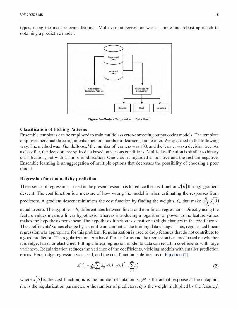
MethodThere were two goals for this research (see Figure 1). The first was to classify the etching patterns basedon rock type and treatment condition. A multi-class algorithm was needed to label the different classes,depending on various conditions. The second goal was predicting the conductivity of the different rock

SPE-200527-MS 5

types, using the most relevant features. Multi-variant regression was a simple and robust approach toobtaining a predictive model.

Figure 1—Models Targeted and Data Used

Classification of Etching PatternsEnsemble templates can be employed to train multiclass error-correcting output codes models. The templateemployed here had three arguments: method, number of learners, and learner. We specified in the followingway. The method was "GentleBoost," the number of learners was 100, and the learner was a decision tree. Asa classifier, the decision tree splits data based on various conditions. Multi-classification is similar to binaryclassification, but with a minor modification. One class is regarded as positive and the rest are negative.Ensemble learning is an aggregation of multiple options that decreases the possibility of choosing a poormodel.

Regression for conductivity predictionThe essence of regression as used in the present research is to reduce the cost function through gradientdescent. The cost function is a measure of how wrong the model is when estimating the responses from

predictors. A gradient descent minimizes the cost function by finding the weights, θj, that make

equal to zero. The hypothesis hθ differentiates between linear and non-linear regressions. Directly using thefeature values means a linear hypothesis, whereas introducing a logarithm or power to the feature valuesmakes the hypothesis non-linear. The hypothesis function is sensitive to slight changes in the coefficients.The coefficients' values change by a significant amount as the training data change. Thus, regularized linearregression was appropriate for this problem. Regularization is used to drop features that do not contribute toa good prediction. The regularization term has different forms and the regression is named based on whetherit is ridge, lasso, or elastic net. Fitting a linear regression model to data can result in coefficients with largevariances. Regularization reduces the variance of the coefficients, yielding models with smaller predictionerrors. Here, ridge regression was used, and the cost function is defined as in Equation (2):

(2)

where is the cost function, m is the number of datapoints, y(i) is the actual response at the datapointi, λ is the regularization parameter, n the number of predictors, θj is the weight multiplied by the feature j,

6 SPE-200527-MS

and hθ(x(i) is the hypothesis. The hypothesis consisted of a combination of Xs multiplied by θs, dependingon the design matrix.

Results and Discussion

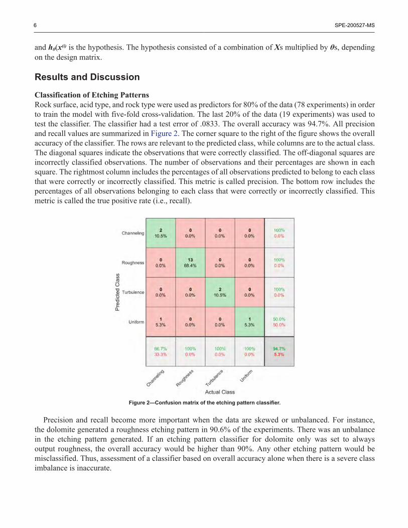
Classification of Etching PatternsRock surface, acid type, and rock type were used as predictors for 80% of the data (78 experiments) in orderto train the model with five-fold cross-validation. The last 20% of the data (19 experiments) was used totest the classifier. The classifier had a test error of .0833. The overall accuracy was 94.7%. All precisionand recall values are summarized in Figure 2. The corner square to the right of the figure shows the overallaccuracy of the classifier. The rows are relevant to the predicted class, while columns are to the actual class.The diagonal squares indicate the observations that were correctly classified. The off-diagonal squares areincorrectly classified observations. The number of observations and their percentages are shown in eachsquare. The rightmost column includes the percentages of all observations predicted to belong to each classthat were correctly or incorrectly classified. This metric is called precision. The bottom row includes thepercentages of all observations belonging to each class that were correctly or incorrectly classified. Thismetric is called the true positive rate (i.e., recall).

Figure 2—Confusion matrix of the etching pattern classifier.

Precision and recall become more important when the data are skewed or unbalanced. For instance,the dolomite generated a roughness etching pattern in 90.6% of the experiments. There was an unbalancein the etching pattern generated. If an etching pattern classifier for dolomite only was set to alwaysoutput roughness, the overall accuracy would be higher than 90%. Any other etching pattern would bemisclassified. Thus, assessment of a classifier based on overall accuracy alone when there is a severe classimbalance is inaccurate.

SPE-200527-MS 7

Regression for conductivity prediction

Dolomite. Data often contain predictors that do not have any relationship with the response. Thesepredictors should not be included in the model. It is better to have a limited number of predictors, yet holdnearly complete variance of the data (Kazakov et al., 2011). One way to select the most relevant predictorsfor response is to repeatedly train the model while adding predictors and monitoring loss. At a specific point,adding more predictors will not increase the accuracy, only calculation time and memory consumption.

The acid type, rock surface, and etching pattern were transformed into dummy variables to make theentire dataset homogeneous as numeric values. For instance, a categorical predictor that contained a numberof categories equal to K was transformed into K-1 predictors of zeros and ones.

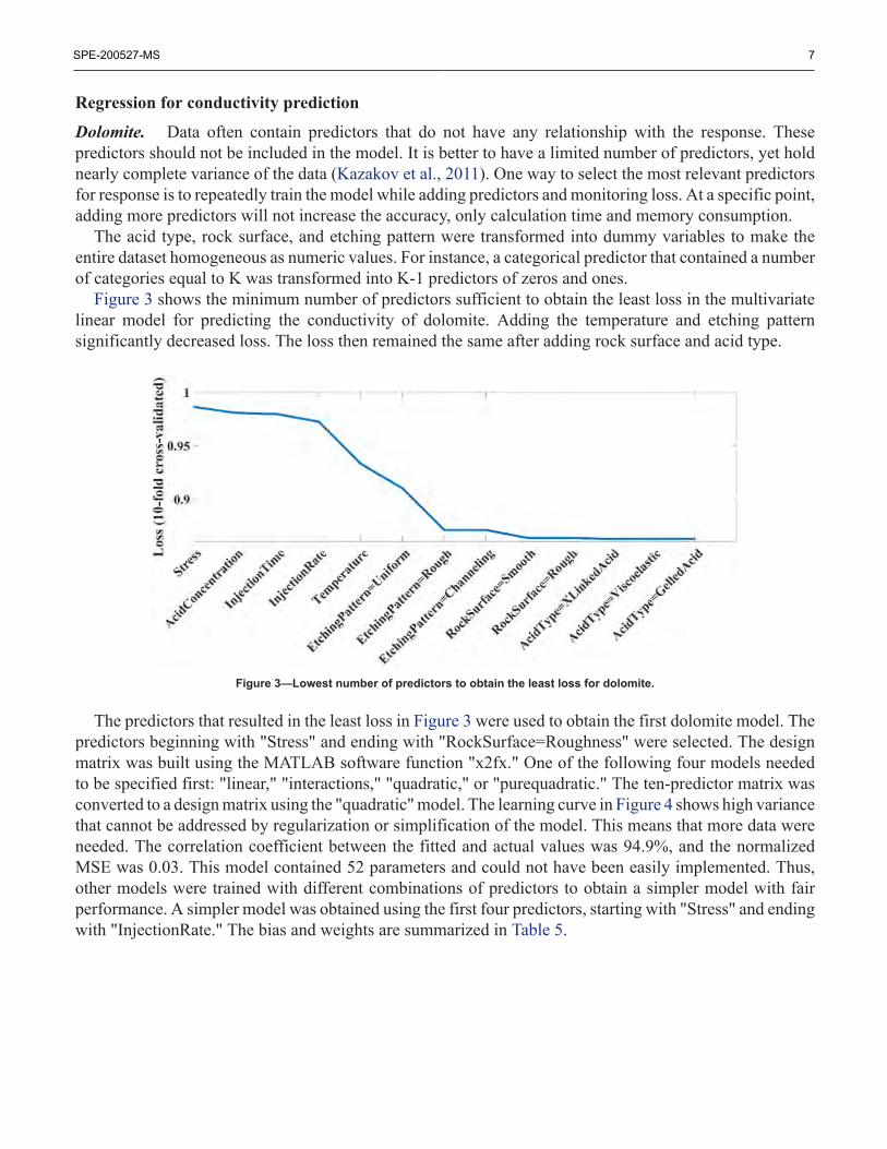
Figure 3 shows the minimum number of predictors sufficient to obtain the least loss in the multivariatelinear model for predicting the conductivity of dolomite. Adding the temperature and etching patternsignificantly decreased loss. The loss then remained the same after adding rock surface and acid type.

Figure 3—Lowest number of predictors to obtain the least loss for dolomite.

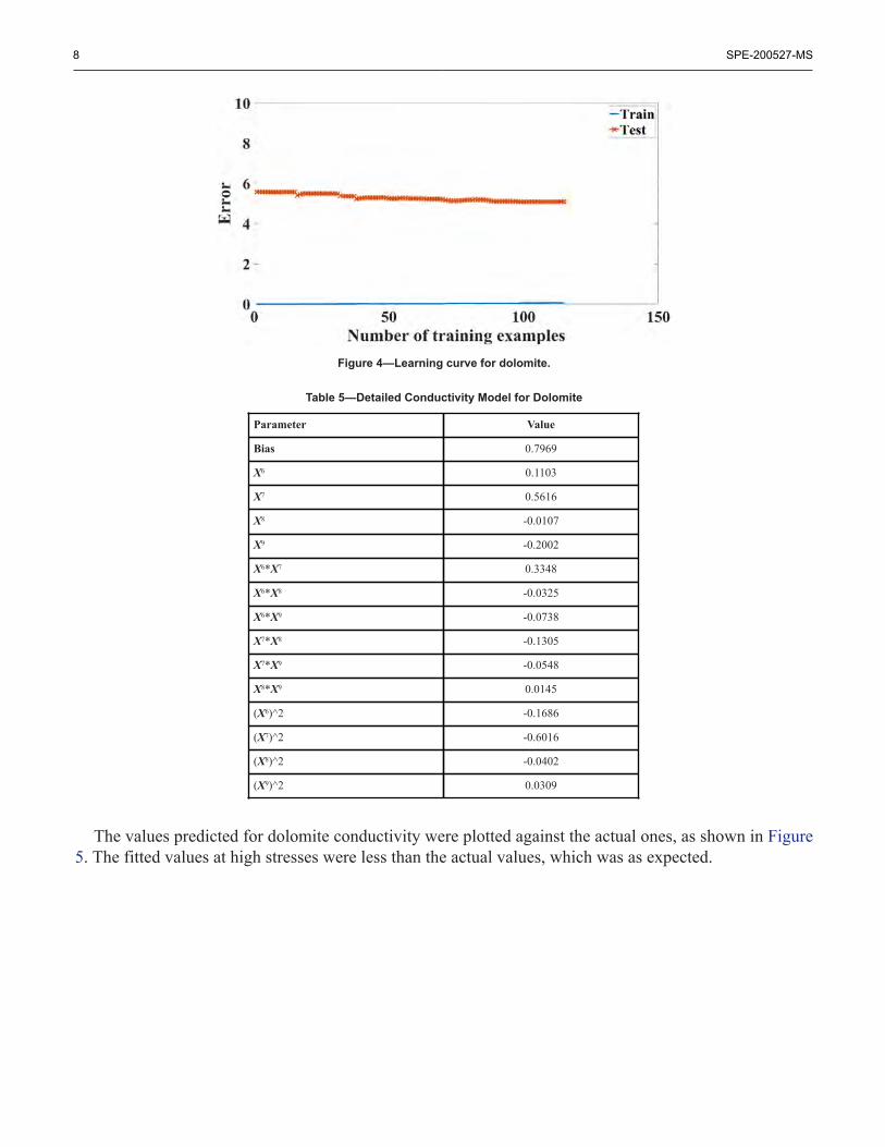
The predictors that resulted in the least loss in Figure 3 were used to obtain the first dolomite model. Thepredictors beginning with "Stress" and ending with "RockSurface=Roughness" were selected. The designmatrix was built using the MATLAB software function "x2fx." One of the following four models neededto be specified first: "linear," "interactions," "quadratic," or "purequadratic." The ten-predictor matrix wasconverted to a design matrix using the "quadratic" model. The learning curve in Figure 4 shows high variancethat cannot be addressed by regularization or simplification of the model. This means that more data wereneeded. The correlation coefficient between the fitted and actual values was 94.9%, and the normalizedMSE was 0.03. This model contained 52 parameters and could not have been easily implemented. Thus,other models were trained with different combinations of predictors to obtain a simpler model with fairperformance. A simpler model was obtained using the first four predictors, starting with "Stress" and endingwith "InjectionRate." The bias and weights are summarized in Table 5.

8 SPE-200527-MS

Figure 4—Learning curve for dolomite.

Table 5—Detailed Conductivity Model for Dolomite

Parameter Value

Bias 0.7969

X6 0.1103

X7 0.5616

X8 -0.0107

X9 -0.2002

X6*X7 0.3348

X6*X8 -0.0325

X6*X9 -0.0738

X7*X8 -0.1305

X7*X9 -0.0548

X8*X9 0.0145

(X6)^2 -0.1686

(X7)^2 -0.6016

(X8)^2 -0.0402

(X9)^2 0.0309

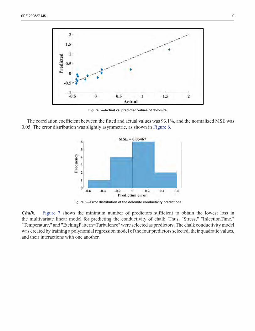
The values predicted for dolomite conductivity were plotted against the actual ones, as shown in Figure5. The fitted values at high stresses were less than the actual values, which was as expected.

SPE-200527-MS 9

Figure 5—Actual vs. predicted values of dolomite.

The correlation coefficient between the fitted and actual values was 93.1%, and the normalized MSE was0.05. The error distribution was slightly asymmetric, as shown in Figure 6.

Figure 6—Error distribution of the dolomite conductivity predictions.

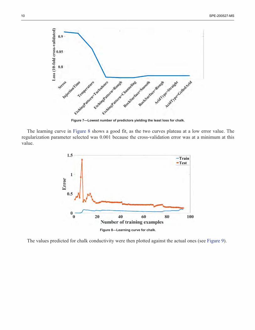
Chalk. Figure 7 shows the minimum number of predictors sufficient to obtain the lowest loss inthe multivariate linear model for predicting the conductivity of chalk. Thus, "Stress," "InlectionTime,""Temperature," and "EtchingPattern=Turbulence" were selected as predictors. The chalk conductivity modelwas created by training a polynomial regression model of the four predictors selected, their quadratic values,and their interactions with one another.

10 SPE-200527-MS

Figure 7—Lowest number of predictors yielding the least loss for chalk.

The learning curve in Figure 8 shows a good fit, as the two curves plateau at a low error value. Theregularization parameter selected was 0.001 because the cross-validation error was at a minimum at thisvalue.

Figure 8—Learning curve for chalk.

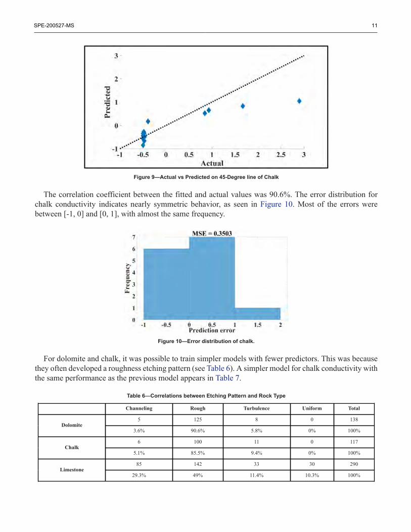
The values predicted for chalk conductivity were then plotted against the actual ones (see Figure 9).

SPE-200527-MS 11

Figure 9—Actual vs Predicted on 45-Degree line of Chalk

The correlation coefficient between the fitted and actual values was 90.6%. The error distribution forchalk conductivity indicates nearly symmetric behavior, as seen in Figure 10. Most of the errors werebetween [-1, 0] and [0, 1], with almost the same frequency.

Figure 10—Error distribution of chalk.

For dolomite and chalk, it was possible to train simpler models with fewer predictors. This was becausethey often developed a roughness etching pattern (see Table 6). A simpler model for chalk conductivity withthe same performance as the previous model appears in Table 7.

Table 6—Correlations between Etching Pattern and Rock Type

Channeling Rough Turbulence Uniform Total

5 125 8 0 138Dolomite

3.6% 90.6% 5.8% 0% 100%

6 100 11 0 117Chalk

5.1% 85.5% 9.4% 0% 100%

85 142 33 30 290Limestone

29.3% 49% 11.4% 10.3% 100%

12 SPE-200527-MS

Table 7—Detailed Conductivity Model for Chalk

Parameter Value

Bias 0.3769

X5 -0.1179

X7 0.2851

X9 -0.3391

X5*X7 -0.0672

X5*X9 -0.0867

X7*X9 0.0232

X5^2 -0.5476

X7^2 -0.0567

X9^2 0.1459

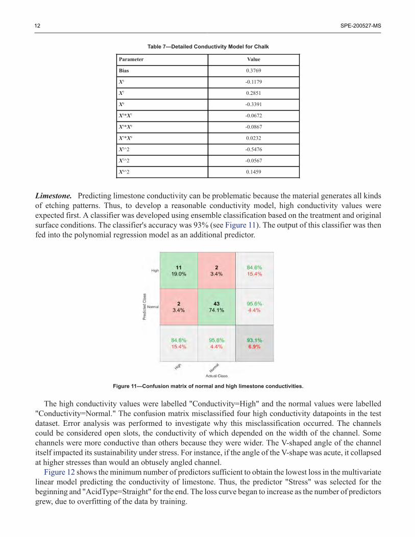
Limestone. Predicting limestone conductivity can be problematic because the material generates all kindsof etching patterns. Thus, to develop a reasonable conductivity model, high conductivity values wereexpected first. A classifier was developed using ensemble classification based on the treatment and originalsurface conditions. The classifier's accuracy was 93% (see Figure 11). The output of this classifier was thenfed into the polynomial regression model as an additional predictor.

Figure 11—Confusion matrix of normal and high limestone conductivities.

The high conductivity values were labelled "Conductivity=High" and the normal values were labelled"Conductivity=Normal." The confusion matrix misclassified four high conductivity datapoints in the testdataset. Error analysis was performed to investigate why this misclassification occurred. The channelscould be considered open slots, the conductivity of which depended on the width of the channel. Somechannels were more conductive than others because they were wider. The V-shaped angle of the channelitself impacted its sustainability under stress. For instance, if the angle of the V-shape was acute, it collapsedat higher stresses than would an obtusely angled channel.

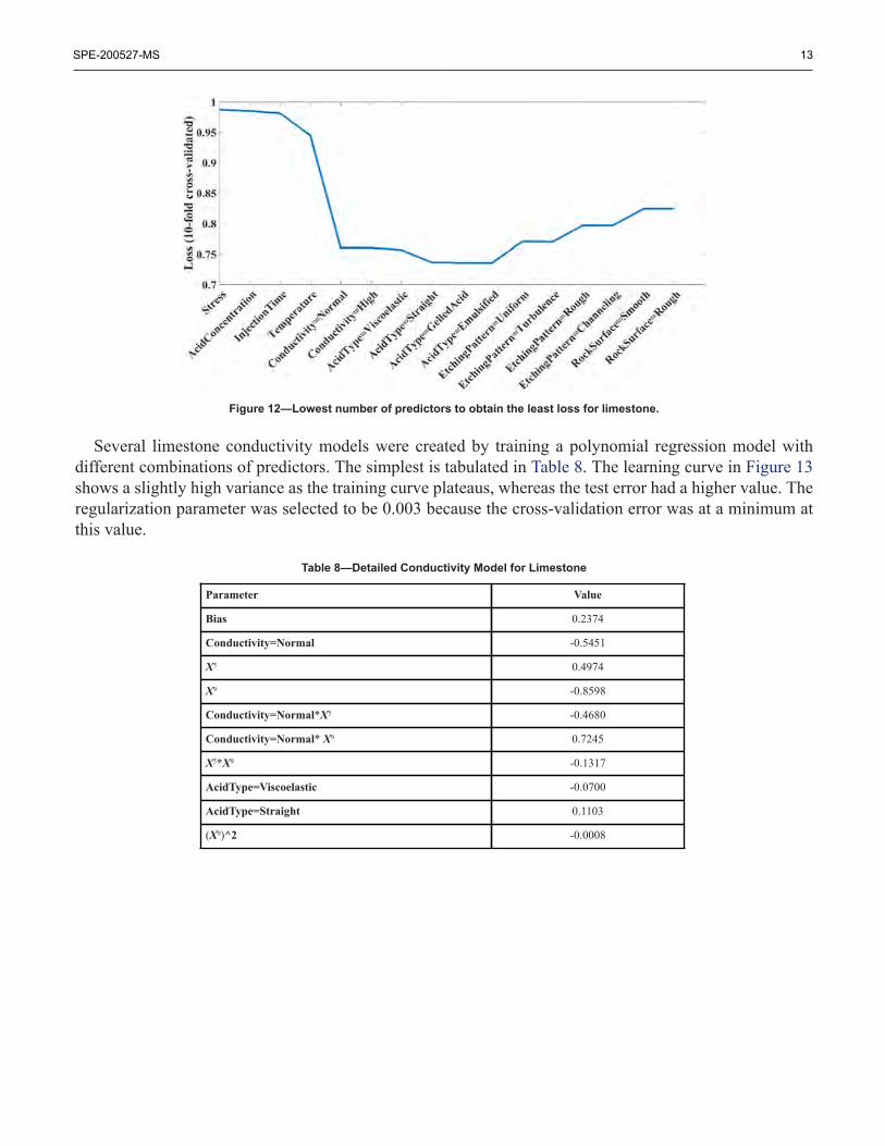
Figure 12 shows the minimum number of predictors sufficient to obtain the lowest loss in the multivariatelinear model predicting the conductivity of limestone. Thus, the predictor "Stress" was selected for thebeginning and "AcidType=Straight" for the end. The loss curve began to increase as the number of predictorsgrew, due to overfitting of the data by training.

SPE-200527-MS 13

Figure 12—Lowest number of predictors to obtain the least loss for limestone.

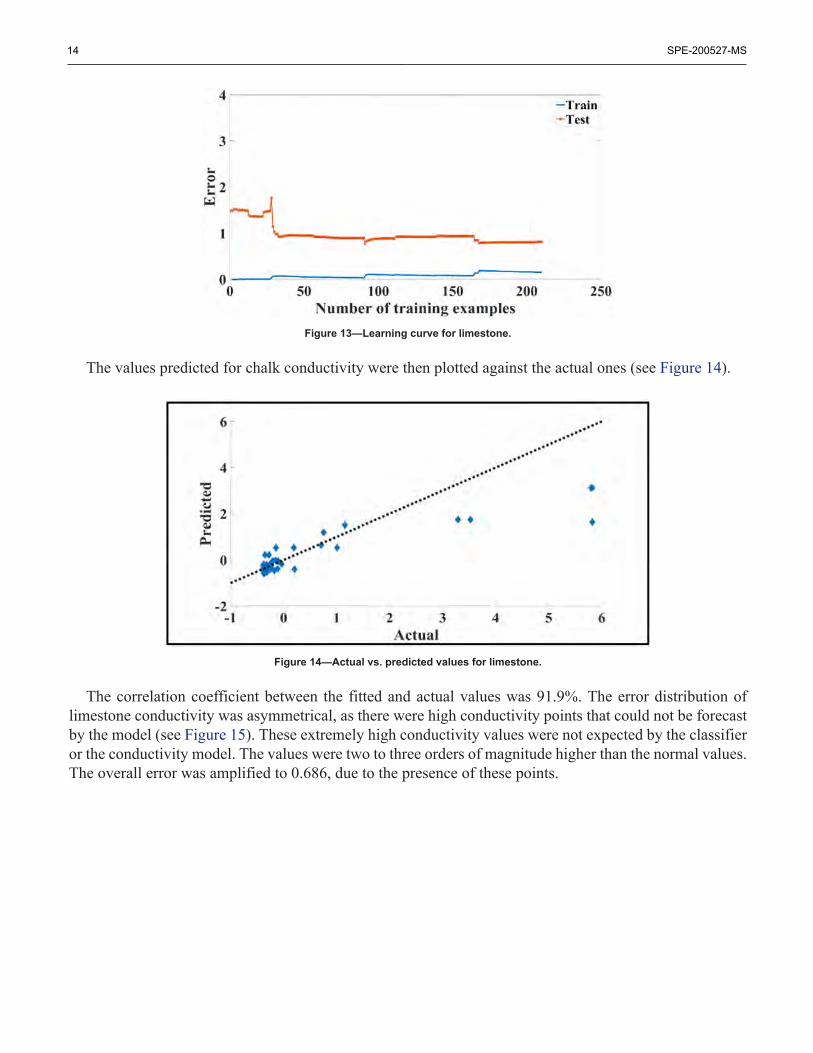
Several limestone conductivity models were created by training a polynomial regression model withdifferent combinations of predictors. The simplest is tabulated in Table 8. The learning curve in Figure 13shows a slightly high variance as the training curve plateaus, whereas the test error had a higher value. Theregularization parameter was selected to be 0.003 because the cross-validation error was at a minimum atthis value.

Table 8—Detailed Conductivity Model for Limestone

Parameter Value

Bias 0.2374

Conductivity=Normal -0.5451

X5 0.4974

X9 -0.8598

Conductivity=Normal*X5 -0.4680

Conductivity=Normal* X9 0.7245

X5*X9 -0.1317

AcidType=Viscoelastic -0.0700

AcidType=Straight 0.1103

(X9)^2 -0.0008

14 SPE-200527-MS

Figure 13—Learning curve for limestone.

The values predicted for chalk conductivity were then plotted against the actual ones (see Figure 14).

Figure 14—Actual vs. predicted values for limestone.

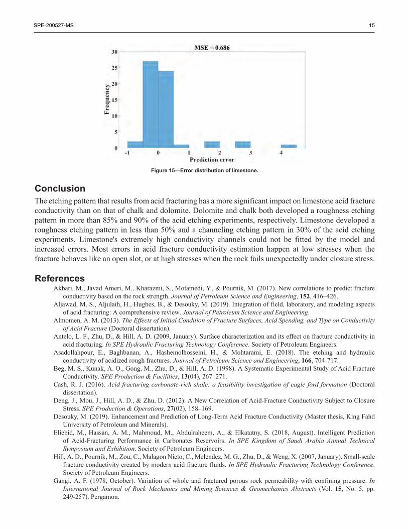
The correlation coefficient between the fitted and actual values was 91.9%. The error distribution oflimestone conductivity was asymmetrical, as there were high conductivity points that could not be forecastby the model (see Figure 15). These extremely high conductivity values were not expected by the classifieror the conductivity model. The values were two to three orders of magnitude higher than the normal values.The overall error was amplified to 0.686, due to the presence of these points.

SPE-200527-MS 15

Figure 15—Error distribution of limestone.

ConclusionThe etching pattern that results from acid fracturing has a more significant impact on limestone acid fractureconductivity than on that of chalk and dolomite. Dolomite and chalk both developed a roughness etchingpattern in more than 85% and 90% of the acid etching experiments, respectively. Limestone developed aroughness etching pattern in less than 50% and a channeling etching pattern in 30% of the acid etchingexperiments. Limestone's extremely high conductivity channels could not be fitted by the model andincreased errors. Most errors in acid fracture conductivity estimation happen at low stresses when thefracture behaves like an open slot, or at high stresses when the rock fails unexpectedly under closure stress.

ReferencesAkbari, M., Javad Ameri, M., Kharazmi, S., Motamedi, Y., & Pournik, M. (2017). New correlations to predict fracture

conductivity based on the rock strength. Journal of Petroleum Science and Engineering, 152, 416–426.Aljawad, M. S., Aljulaih, H., Hughes, B., & Desouky, M. (2019). Integration of field, laboratory, and modeling aspects

of acid fracturing: A comprehensive review. Journal of Petroleum Science and Engineering.Almomen, A. M. (2013). The Effects of Initial Condition of Fracture Surfaces, Acid Spending, and Type on Conductivity

of Acid Fracture (Doctoral dissertation).Antelo, L. F., Zhu, D., & Hill, A. D. (2009, January). Surface characterization and its effect on fracture conductivity in

acid fracturing. In SPE Hydraulic Fracturing Technology Conference. Society of Petroleum Engineers.Asadollahpour, E., Baghbanan, A., Hashemolhosseini, H., & Mohtarami, E. (2018). The etching and hydraulic

conductivity of acidized rough fractures. Journal of Petroleum Science and Engineering, 166, 704-717.Beg, M. S., Kunak, A. O., Gong, M., Zhu, D., & Hill, A. D. (1998). A Systematic Experimental Study of Acid Fracture

Conductivity. SPE Production & Facilities, 13(04), 267–271.Cash, R. J. (2016). Acid fracturing carbonate-rich shale: a feasibility investigation of eagle ford formation (Doctoral

dissertation).Deng, J., Mou, J., Hill, A. D., & Zhu, D. (2012). A New Correlation of Acid-Fracture Conductivity Subject to Closure

Stress. SPE Production & Operations, 27(02), 158–169.Desouky, M. (2019). Enhancement and Prediction of Long-Term Acid Fracture Conductivity (Master thesis, King Fahd

University of Petroleum and Minerals).Eliebid, M., Hassan, A. M., Mahmoud, M., Abdulraheem, A., & Elkatatny, S. (2018, August). Intelligent Prediction

of Acid-Fracturing Performance in Carbonates Reservoirs. In SPE Kingdom of Saudi Arabia Annual TechnicalSymposium and Exhibition. Society of Petroleum Engineers.

Hill, A. D., Pournik, M., Zou, C., Malagon Nieto, C., Melendez, M. G., Zhu, D., & Weng, X. (2007, January). Small-scalefracture conductivity created by modern acid fracture fluids. In SPE Hydraulic Fracturing Technology Conference.Society of Petroleum Engineers.

Gangi, A. F. (1978, October). Variation of whole and fractured porous rock permeability with confining pressure. InInternational Journal of Rock Mechanics and Mining Sciences & Geomechanics Abstracts (Vol. 15, No. 5, pp.249-257). Pergamon.

16 SPE-200527-MS

Gong, M. (1997). Mechanical and hydraulic behavior of acid fractures: experimental studies and mathematical modeling(Doctoral dissertation, University of Texas at Austin).

Jin, X., Zhu, D., Hill, A. D., & McDuff, D. (2019, January 29). Effects of Heterogeneity in Mineralogy Distribution onAcid Fracturing Efficiency. Society of Petroleum Engineers. doi: 10.2118/194377-MS

Kamali, A., & Pournik, M. (2015, January). Rough Surface Closure–A Closer Look at Fracture Closure and ConductivityDecline. In ISRM Regional Symposium-EUROCK 2015. International Society for Rock Mechanics and RockEngineering.

Kamali, A., & Pournik, M. (2016). Fracture closure and conductivity decline modeling – Application in unpropped andacid etched fractures. Journal of Unconventional Oil and Gas Resources, 14, 44–55.

Kazakov, N., & Miskimins, J. L. (2011, January). Application of multivariate statistical analysis to slickwater fracturingparameters in unconventional reservoir systems. In SPE Hydraulic Fracturing Technology Conference. Society ofPetroleum Engineers.

Lu, C., Bai, X., Luo, Y., & Guo, J. (2017). New study of etching patterns of acid-fracture surfaces and relevant conductivity.Journal of Petroleum Science and Engineering, 159, 135–147.

Melendez, M. G., Pournik, M., Zhu, D., & Hill, A. D. (2007, January). The effects of acid contact time and the resultingweakening of the rock surfaces on acid fracture conductivity. In European Formation Damage Conference. Societyof Petroleum Engineers.

Motamedi-Ghahfarokhi, Y., Ameri Shahrabi, M. J., Akbari, M., & Pournik, M. (2018). New correlations to predict fractureconductivity based on the formation lithology. Energy Sources, Part A: Recovery, Utilization, and EnvironmentalEffects, 40(13), 1663-1673.

Nierode, D. E., & Kruk, K. F. (1973, January). An evaluation of acid fluid loss additives retarded acids, and acidizedfracture conductivity. In Fall Meeting of the Society of Petroleum Engineers of AIME. Society of Petroleum Engineers.

Nieto, C. M., Pournik, M., & Hill, A. D. (2008). The texture of acidized fracture surfaces: implications for acid fractureconductivity. SPE Production & Operations, 23(03), 343-352.

Nino Penaloza, A. (2013). Experimental Study of Acid Fracture Conductivity of Austin Chalk Formation (Doctoraldissertation).

Pournik, M. (2008). Laboratory-scale fracture conductivity created by acid etching. Texas A&M University.Pournik, M., Zhu, D., & Hill, A. D. (2009, January). Acid-fracture conductivity correlation development based on acid-

etched fracture characterization. In 8th European Formation Damage Conference. Society of Petroleum Engineers.Pournik, M., Gomaa, A. M., & Nasr-El-Din, H. A. (2010, January). Influence of acid-fracture fluid properties on acid-

etched surfaces and resulting fracture conductivity. In SPE International Symposium and Exhibition on FormationDamage Control. Society of Petroleum Engineers.

Pournik, M., Li, L., Smith, B. T., & Nasr-El-Din, H. A. (2013). Effect of acid spending on etching and acid-fractureconductivity. SPE Production & Operations, 28(01), 46-54.

Ruffet, C., Fery, J. J., & Onaisi, A. (1998). Acid Fracturing Treatment: a Surface Topography Analysis of Acid EtchedFractures to Determine Residual Conductivity. SPE Journal, 3(02), 155–162.

Van Domelen, M. S., Gdanski, R. D., & Finley, D. B. (1994, January). The application of core and well testing to fractureacidizing treatment design: a case study. In European Production Operations Conference and Exhibition. Society ofPetroleum Engineers.

Walsh, J. B. (1981, October). Effect of pore pressure and confining pressure on fracture permeability. In InternationalJournal of Rock Mechanics and Mining Sciences & Geomechanics Abstracts (Vol. 18, No. 5, pp. 429-435). Pergamon.

Williams, B. B., Gidley, J. L., & Schechter, R. S. (1979). Acidizing Fundamentals, Henry L. Doherty Memorial Fund ofAIME, Society of Petroleum Engineers of AIME, New York.

Zou, C. (2006). Development and Testing of an Advanced Acid Fracture Conductivity Apparatus. 2006. 59 f. Master ofScience Thesis-Texas A&M University.