SPE-187137-MS

Seismic Inversion Based SRV and Reserves Estimation for Shale Plays

Saurabh Sinha, Kurt J. Marfurt, Deepak Devegowda, and Rafael Pires de Lima, University of Oklahoma; SumitVerma, University of Texas, Permian Basin

Copyright 2017, Society of Petroleum Engineers

This paper was prepared for presentation at the SPE Annual Technical Conference and Exhibition held in San Antonio, Texas, USA, 9-11 October 2017.

This paper was selected for presentation by an SPE program committee following review of information contained in an abstract submitted by the author(s). Contentsof the paper have not been reviewed by the Society of Petroleum Engineers and are subject to correction by the author(s). The material does not necessarily reflectany position of the Society of Petroleum Engineers, its officers, or members. Electronic reproduction, distribution, or storage of any part of this paper without the writtenconsent of the Society of Petroleum Engineers is prohibited. Permission to reproduce in print is restricted to an abstract of not more than 300 words; illustrations maynot be copied. The abstract must contain conspicuous acknowledgment of SPE copyright.

AbstractEstimation of stimulated rock volume (SRV) is the cornerstone offield development planning in shalereservoirs. The EUR has a first order dependency on the SRV and therefore its estimation is extremelycritical for field development.

In this paper, we propose a methodology to estimate the SRV and hence the EUR for a shale reservoirusing seismic data, flow and geomechanical simulation. The backbone of our methodology is seismicinversion coupled with geomechanical simulation. We apply our technique to data acquired from the Barnettshale.

In this work, we first use 3D seismic and sonic logs to perform pre-stack seismic inversion. Then, wederive the distribution of Poisson's ratio and Young's modulus in the area of interest (AOI). We constrainthe porosity in our geo cellular model using a rock type model. Our rock type model for this work is basedon k-means clustering on multi-well log analysis.

We modeled a well in the AOI for which microseismic data is available. Weused a coupledflow andgeomechanical simulator to mimic the fracturing process and the fluid volumes injected during the actualcompletion of the well. For geomechanical coupling, we used Barton-Bandis model in seismic inversion-derived Young's modulus and Poisson's ratio 3D volumes. Next, we compare our results with the SRVobtained by an analysis of microseismic data. We reconcile differences in the model-derived SRV and thencalibrate the resulting flow model and use the history-matched model for forecasting production.

Our results indicate an excellent match on SRV and therefore production data. Because we usevariablegeomechanical parameters along the lateral, we observe irregular SRV's and drainage areas consistent withthe microseismic data. Our methodology for predicting microseismic can be used for asset evaluation,acreage prioritization and to optimize the completion design in unconventional plays.

IntroductionFigure 1a shows the EUR plotted against the SRV derived from a dual-porosity reservoir simulation modelfor a shale well completed in a naturally fractured shale reservoir such as the Barnett shale. The reservoirmodel is specified to be 7000 ft. deep with a median porosity of 14% and a permeability of 1000 nD.Assuming that no other variables change, the EUR increases with the SRV. In reality, this linear trend may

2 SPE-187137-MS

not necessarily be true because of other factors such as improper proppant placement and geomechanicaleffects over time. However, the model does illustrate the significance of the SRV to enhance the EUR/well.

Figure 1—a) Model-predicted EUR versus SRV. The EUR strongly depends on the SRV. The modelis shown in Figure 1b. b) Complex fracture network in the model and enhanced permeability zones.

Production forecasting and estimation of reserves is the key challenge in unconventional fielddevelopment. 3D seismic surveys provide high value in understanding the reservoir and helps operators to:

a. Identify and develop high value acreageand prioritize which part of the acreage be developed first.b. Optimize completion design for wells: Knowing SRV's ahead of time, critical changes can be made in

areawise completion design to maximize recovery from the well. For example, for wells in differentsections of the play associated with different fluid types.

c. Optimize the well spacing: If the extent of SRV is known along with the geometry, optimal wellspacing can be implemented in field to minimize well interference and maximize recovery factors.

d. Accurate reserves reporting in underdeveloped portions in the reservoir.

The information derived from 3D seismicanalysis may help operators achieve the above-mentionedobjectives prior to drilling. Moreover seismic derived properties are available at a much finer intervalthan well spacing. Although, the resolution depends on the acquisition geometry, well control is likely notavailable at such finer intervals.

Previous attempts of correlating production with 3D seismic do not include the direct coupling of physicalproperties with constitutive equations. For example, Zhang et al. (2015) elaborated the use of pre-stackinversion and Rickman's equation (Rickman et al., 2008)to estimate Poisson's ratio, Young modulus andbrittleness. Perez Altamar and Marfurt (2015) utilized the same concept and added lambda-rho and mu-rho

SPE-187137-MS 3

to better identify the brittle and ductile areas. Verma et al. (2016) further extended the concept of brittlenessand added total organic carbon (TOC) from Passey's method to identify the sweet spots in Barnett shale.

Unfortunately, all the previous methods, while promising, do not use any physical law coupling withfluid flow. This leads to qualitative correlation with cumulative produced volumes or EUR's that do notprovide any quantitative relationships. Consequently, sensitivity analyses to different well designs, fracturedesigns and spacing is challenging.

Reservoir engineers rely on the use of decline curve analysis, analytical methods and reservoir simulationto estimate EUR's. Lee and Sidle (2010) discuss the methods of decline curve analysis while Stalgorova andMattar (2013) document some of the analytical methods. Coupling of flow simulations with geomechanicsis discussed in detail by Ji and Sullivan (2009). Amongst these methods, reservoir simulation is the mostrigorous and provides the capability to perform sensitivity analyses as well as the testing different rockfailure criterion.

Methodology

Development of geological modelWe use a 3D seismic survey from Barnett shale as shown in Figure 2 highlighting the areal extent of thesurvey and the well control available from pilot wells in the area. The survey consists of 366 inlinesand 270crosslines separated by an interval of 110 ft. in both cases. The total survey is thus 7.6 miles by 5.6 miles.The survey has 27 wells with well logs. The location of these wells is shown in Figure 2 along with thepicked Viola Limestone surface indepth domain. The sampling rate used in the survey is 2 ms.

Figure 2—Areal extent of the seismic survey and the available wells. The survey is 7.6 miles by 5.6 milesand consists of 366 inlines and 270 crosslines. The survey has good well control with 27 pilot wells in the

area. The horizon overlay with the inlines and crosslines is the top of Viola limestone after depth conversion.

The formation of interest is lower Barnett because most of the wells are completed in this zone. Thelower Barnett is relatively flat in our area of interest (AOI) with minimum to no fault planes. First, we pickthe seismic horizons in time domain and then convert them into depth domain using a linear velocity model.The Lower Barnett in our area has a thickness of 300- 350 ft.

4 SPE-187137-MS

Figure 3 shows an example stratigraphic cross section from the wells in our area. The stratigraphiccross section consists of Viola Limestone, Lower Barnett, Forestburg limestone and Upper Barnett. TheForestburg limestone is squeezed between lower and upper Barnett and thins out towards the SE sectionin the area (Verma et al. 2016)).

Figure 3—Stratigraphic cross section in the area. Forestburg limestone is sandwiched betweenupper and lower Barnett. Most wells are completed in lower Barnett in this area. The lower Barnettthickness varies from ~ 300 - 350 Ft. in this area. Horizon 1 (H1) is the top of upper Barnett, H2 is

the top of Forestburg limestone, H3 is the top of lower Barnett and H4 is the top of Viola limestone.

We used the pre-stack inversion to derive Young's modulus (λ) and Poisson's ratio (μ) (Zhang et al. 2015).The results of Poisson's ratio and Young's modulus along with seismic amplitude is shown in Figure 4. Itcan be observed from Figure 4 that the range of Young's modulus in our AOI varies between 60-70 GPaand Poisson's ratio varies between 0.23-0.30. These values are variable with depth and agree with thosereported by Vermylen (2011) and Sone (2012) from laboratory measurements.

SPE-187137-MS 5

Figure 4—a) Poisson's Ratio on the top of lower Barnett shale b) Young's modulus on the top of lowerBarnett shale. The Poisson's ratio in Lower Barnett varies from 0.23 -0.30 and Young's modulus varies from60-70 GPa. The well with microseismic data is in the NE portion of the survey and is shown with a red circle.

Rock-Type ModelFor rock typing we used k-means clustering based on the gamma ray, sonic and bulk density log. We identifya total of 6 rock types in the upper and 6 rock types in the lower Barnett. Figure 5a shows the "elbow-point"plot which allowed us to determine the number of clusters by defining the sum of squares between eachcluster. The change in the slope starts around 4 clusters, but the ideal number may be anywhere between 4and 8 clusters. Figure 5b shows the clustersplotted with the first two principal components.

We calculate these rock types in every well and derived the variograms for the facies model. We then usesequential indicator simulation (SIS) to distribute these facies in the reservoir. Figure 6 show the distributionof these rock types at top of the lower Barnett. We then use these rock types to constrain the density porosityderived from these wells. We use sequential gaussian simulation (SGS) to populate rock type constrainedporosity. Figure 6 shows the facies and Figure 7 shows the porosity cross section at the top of lower Barnett.

6 SPE-187137-MS

Figure 5—a) Number of clusters from k-meansb) Cluster plot using principal components

SPE-187137-MS 7

Figure 6—a) Rock type model at the top of lower Barnett. Rock types are based on k- meansclustering of well log data from bulk density, sonic and gamma ray logs. b) shows the histogramof porosity for different facies and their respective percentages in lower Barnett. The histogramshows good correlation between the log-derived values of porosity and the upscaled cell values.

Figure 7—Rock type constrained porosity in lower Barnett shale and distribution of porosity withinBarnett Shale. The porosity varies from 3% to 27% in lower Barnett with a median porosity of 16%.

8 SPE-187137-MS

Completion Details and In-Situ StressThe well in the model has ~ 2000 ft. lateral length (perforated and completed) with 100 ft stage spacingand is completed with 20 stages. The design pumping rate is 64 BPM cluster. Microseismic is recorded inthe well with an observation well to the south-east of it. The well is a single well completion with just onewell on the PAD and without zipper fracturing.

To calculate the pore pressure, we used mud weight gravity in the region where there is no lost circulationor gas influx. We calculated pore pressure gradient in our area as 0.475 psi/ft which corresponds to the valueof 0.48 psi/ft reported by Vermylen (2011). To calculate the vertical stress, we integrate the bulk densitylog. We do not have formation image logs or formation fracturing tests to calculate the maximum (Shmax)and minimum (Shmin) horizontal stresses and orientation.

Therefore we choose the first fracturing stage shut in pressure to initialize Shmin. Due to excessive frictionlosses such as proppant and gel viscous flow as well as dynamic stress changes we avoid the use of otherstages to calculate Shmin. We show this pressure in Figure 8.

Figure 8—Fracturing report of the well in which microseismic is obtained and is modeled in this study. It can be observed thatthe ISIP for the first stage is ~3600-3700 Psi and hence is used as Shmin. (Image modified from that provided by the operator).

The Barnett has been reported as being characterized by relatively low stress anisotropy (Vermylen, 2011)and therefore we assume Shminto be slightly lesser (by 100 psi) than Shmax. Table 1 summarizes these values.

To propagate the fractures in the model, we use the Barton-Bandis model (Bandis et al. 1983) with adual porosity assumption. The numerical groundwork for implementing the methodology is described byNghiem et al. (2004). Figure 9 shows the conceptual background for the model. As injection continues,pore pressure increases and hence effective normal stress decreases. At the effective opening stress for thenatural fractures, the fractures open and are characterized by a high fracture conductivity. The permeabilitydeclines as the effective stress increases again during production due to a decrease in pore pressure.

SPE-187137-MS 9

Figure 9—Modified Barton- Bandis model used in this study. The image is modified after Sinha et al. (2017) (originalimage modified from Tran et al. (2009)). As the injection continues the effective normal stress (overburden stress– pore pressure) decreases and at point of rock failure there is a sudden increase in permeability. After injection

stops, the permeability decreases semi-logarithmically and stabilizes at a residual permeability of fractures.We have used this residual permeability as a history matching parameter for the long-term production behavior

We usethe fracturing schedule shown in Figure 8 to inject the fracturing water from toe towards heelin 20 stages. As the fracture opening stress is reached, the fractures retain some portion of the initial highpermeability value following an initial period of production. The enhanced permeability then follows asemi-logarithmic decline and the fracture eventually retains a minimum permeability that explains the long-term production behavior (The permeability model is shown in Figure 9). We have assumed an isotropichorizontal reservoir matrix permeability before fracturing.

Table 1—Parameters used for stress initialization

Parameter Value

Initial fracture aperture 0.01 Ft.

Initial fracture stiffness 2.52 E+06

Initial fracture opening stress (limiting case) 3000 Psi

Initial hydraulic fracture permeability 25000 mD

Fracture closure permeability 20000 mD

Initial fracture permeability, after initial production 15000 mD

Biot's coefficient 0.8

Maximum (Shmax)and minimum effective stresses (Shmin) 3700 Psi and 3600 Psi

Vertical effective stress 4340 Psi

History MatchingThe well is completed in the dry gas window of the Barnett hence, our model is assumed to contain onlysingle-phase methane for the fluid model. We use the residual permeability in Barton-Bandis model as thehistory matching parameter to match the gas volumes. We do not have daily production for the wells andtherefore used public information from the website Drillinginfo®, for the monthly allocated production forthis well.

10 SPE-187137-MS

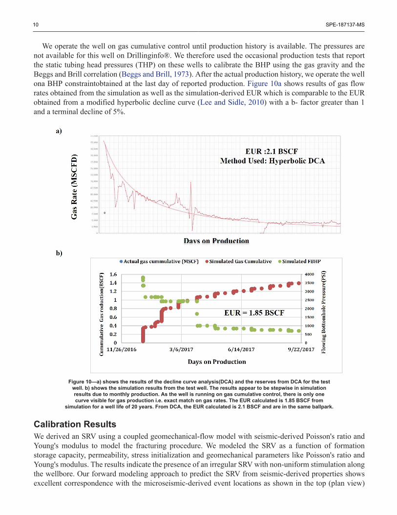
We operate the well on gas cumulative control until production history is available. The pressures arenot available for this well on Drillinginfo®. We therefore used the occasional production tests that reportthe static tubing head pressures (THP) on these wells to calibrate the BHP using the gas gravity and theBeggs and Brill correlation (Beggs and Brill, 1973). After the actual production history, we operate the wellona BHP constraintobtained at the last day of reported production. Figure 10a shows results of gas flowrates obtained from the simulation as well as the simulation-derived EUR which is comparable to the EURobtained from a modified hyperbolic decline curve (Lee and Sidle, 2010) with a b- factor greater than 1and a terminal decline of 5%.

Figure 10—a) shows the results of the decline curve analysis(DCA) and the reserves from DCA for the testwell. b) shows the simulation results from the test well. The results appear to be stepwise in simulationresults due to monthly production. As the well is running on gas cumulative control, there is only onecurve visible for gas production i.e. exact match on gas rates. The EUR calculated is 1.85 BSCF from

simulation for a well life of 20 years. From DCA, the EUR calculated is 2.1 BSCF and are in the same ballpark.

Calibration ResultsWe derived an SRV using a coupled geomechanical-flow model with seismic-derived Poisson's ratio andYoung's modulus to model the fracturing procedure. We modeled the SRV as a function of formationstorage capacity, permeability, stress initialization and geomechanical parameters like Poisson's ratio andYoung's modulus. The results indicate the presence of an irregular SRV with non-uniform stimulation alongthe wellbore. Our forward modeling approach to predict the SRV from seismic-derived properties showsexcellent correspondence with the microseismic-derived event locations as shown in the top (plan view)

SPE-187137-MS 11

and bottom (cross-sectional view) panels of Figure 11. Figure 11a shows the enhanced permeability regionssurrounding the wellbore that is predicted from the forward modeling approach showing good correlationwith the microseismic event locations in Figure 11b. Figures 11c and 11d show the same with in a cross-sectional view. The grid boundary is shown in Figure 11a in a maroon square box. The fracture growth isupwards with more stimulation in the heels and less towards the toe side of the lateral as seen in Figure 11c.There is more stimulation on one side of the lateral than the other due to irregular failure criterion (Young'smodulus and Poisson's ratio maps). We also see highly conductive fractures in the middle portion of thereservoir which is reflected in microseismic events density (Figure 11d).

Figure 11—a) Permeability mapafter the stimulation b) Top view of the actual stimulation treatment microseismic(image provided by the operator) c) I-K view of the stimulation d) I-K view of the actual stimulation microseismic

(image provided by the operator). Figure (a) show a high area of permeability away from the wellbore which cannotbe predicted without a spatial gradation in geomechanical and petrophysical properties. Figure (a) also showthe boundary of the finite element geomechanical grid causing some of the boundary effects. There is a zoneof no stimulation in the middle of the lateral which is not reflected in actual seismic and could be due to some

natural fractures or grid sizing. Figure (c) show more conductive SRV at the middle of the lateral and diminishingconductivity away from the wellbore. Figure (d) show higher microseismic density in the middle section of the

lateral and microseismic event density fading away from the wellbore consistent to the observation in Figure (c).

The initial production is matched by tuning the initialvalue of fracture conductivity and the longer termproduction is matched by calibrating the gradual logarithmic declining fracture conductivity in the Barton-

12 SPE-187137-MS

Bandis model. We observe a general trend of permeability diminishing away from the wellbore but alsomany regions of high permeability away from the wellbore. This observation differs from the generalassumption thatfracture permeability diminishesaway from the wellbore. Our results show that duringproduction the drainage volumes may encompass regions of high permeability instead of progressivelymoving towards lower permeability regions and thisshould be reflected in the flowing material balance plotssuggested by Suliman et al. (2013) and Samandarli et al. (2011).

These high permeability areas can also explain the gradual flattening of decline (as seen in Figure 10a)and b-factors for DCA in some wells contrary to what is expected because the well continues to drain higherpermeability regions at a later period.

ConclusionsThe methodology presented in our paper presents a promising approach to utilize 3D seismic data,microseismic analyses and well-log-derived 3D property models to match production history and predictEUR. The procedure is summarized below:

1. Comparison of microseismic-derived SRV on to SRV predicted from a seismic-derived 3D model ofYoung's Modulus and Poisson's ratio.

2. Utilize the calibrated SRV model in a coupled geomechanical-flow model to match production historyby adjusting fracture conductivities.

The advantage of our approach is that the SRV can be predicted with a high degree of confidence priorto fracturing using 3D seismic data. Although the SRV can be inferred solely from microseismic data asshown by Sinha (2017) and Suliman et al. (2013), our approach allows us to predict the anticipated SRVprior to drilling or fracturing thereby providing better controls on the EUR.

In our study, we observed SRV consistent with microseismic data and hence we are able to forecast EURreliably. We can also quantitatively infer high permeability enhanced fracturing zones and provide a viableway to correlate microseismic event density with the permeability.

AcknowledgementsWe would like to thank Attribute Assisted Seismic Processing & Interpretation at The Universityof Oklahoma (AASPI) for providing funding for this project. We would also like to thank CGG,

Schlumbergerand Computer Modeling Group (CMG) for their generous donation of software licenses.Finally, we would like to extend ourgratitude to Devon Energy for the dataset for this project. Special

thanks to K. Patel and Tanh Nguyen from Computer Modelling Group for their technical support for thisproject.

NomenclatureEUR –Expected ultimate recoverySRV – Stimulated Rock VolumeShmax – Maximum horizontal stressShmin – Minimum horizontal stress

DCA – Decline curve analysisFBHP – Flowing bottomhole pressure

ReferencesBandis, S. C., A. C. Lumsden, and N. R. Barton. 1983. "Fundamentals of Rock Joint Deformation." International Journal

of Rock Mechanics and Mining Sciences and 20 (6): 249–68. doi:10.1016/0148-9062(83)90595-8.Beggs, H. D., and Brill, J. P., (1973). A study of two-phase flow in inclined pipes. Trans. AIME, 255, p. 607

SPE-187137-MS 13

Ji, Lujun, Antonin Settari, and Richard B Sullivan. 2009. "A Novel Hydraulic Fracturing Model Fully Coupled WithGeomechanics and Reservoir Simulation." SPE Journal 14 (3): 423–30. doi:10.2118/110845-PA.

Lee, W J, A Texas, and R E Sidle. 2010. "Gas Reserves Estimation in Resource Plays." SPE 130102, no. February: 23–25.Nghiem, Long, Peter Sammon, Jim Grabenstetter, and Hiroshi Ohkuma. 2004. "Modeling CO2 Storage in Aquifers with

a Fully-Coupled Geochemical EOS Compositional Simulator." Proceedings of SPE/DOE Symposium on ImprovedOil Recovery. doi:10.2118/89474-MS.

Perez Altamar, Roderick, and Kurt J. Marfurt. 2015. "Identification of Brittle/ductile Areas in Unconventional ReservoirsUsing Seismic and Microseismic Data: Application to the Barnett Shale." Interpretation 3 (4): T233–43. doi:10.1190/INT-2013-0021.1.

Rickman, Rick, Michael J. Mullen, James Erik Petre, William Vincent Grieser, and Donald Kundert. 2008. "A PracticalUse of Shale Petrophysics for Stimulation Design Optimization: All Shale Plays Are Not Clones of the Barnett Shale."SPE Annual Technical Conference and Exhibition, no. Wang: 1–11. doi:10.2118/115258-MS.

Samandarli, Orkhan, Hasan Al-ahmadi, Robert a Wattenbarger, and a Texas. 2011. "A New Method for History Matchingand Forecasting Shale Gas Reservoir Production Performance with a Dual Porosity Model." Society, no. 2010: 1–138.doi:10.2118/144335-MS.

Sone, Hiroki. 2012. "Mechanical Properties of Shale Gas Reservoir Rocks and Its Relation to the in-Situ Stress VariationObserved in Shale Gas Reservoirs." Vasa 128 (March): 1–247. doi:10.1017/CBO9781107415324.004.

Sinha, S., Devegowda, D., & Deka, B. (2017, April 23). Quantification of Recovery Factors in Downspaced Wells:Application to the Eagle Ford Shale. Society of Petroleum Engineers. doi:10.2118/185748-MS

Stalgorova, E, L Mattar, I H S Fekete, and Reservoir Solutions. 2013. "SPE 167191 Analytical Modeling forGeomechanical Changes in Multi-Frac Completions", no. November: 5–7.

Suliman, B., R. Meek, R. Hull, H. Bello, D. Portis, and P. Richmond. 2013. "Variable Stimulated Reservoir Volume (SRV)Simulation: Eagle Ford Shale Case Study." Spe 164546, 13. doi:10.2118/164546-MS.

Tran, David, Vijay Shrivastava, Long Nghiem, and Bruce Kohse. 2009. "Geomechanical Risk Mitigation for CO2Sequestration in Saline Aquifers." Proceedings of SPE Annual Technical Conference and Exhibition, 1–18.doi:10.2118/125167-MS.

Verma, Sumit, Tao Zhao, Kurt J. Marfurt, and Deepak Devegowda. 2016. "Estimation of Total Organic Carbon andBrittleness Volume." Interpretation 4 (3): T373–85. doi:10.1190/INT-2015-0166.1.

Vermylen, John P. 2011. "Geomechanical Studies of the Barnett Shale, Texas, USA." Stanford University.Zhang, Bo, Tao Zhao, Xiaochun Jin, and Kurt J. Marfurt. 2015. "Brittleness Evaluation of Resource Plays by Integrating

Petrophysical and Seismic Data Analysis." Interpretation 3 (2): T81–92. doi:10.1190/INT-2014-0144.1.