SPE-184822-MS

Shale Analytics: Making Production and Operational Decisions Based on Facts: A Case Study in Marcellus Shale Mohaghegh, S. D.1, 2, Gaskari, R.1, Maysami, M.1

1Intelligent Solutions, Inc. 2West Virginia University Copyright 2017, Society of Petroleum Engineers This paper was prepared for presentation at the SPE Hydraulic Fracturing Technology Conference and Exhibition held in The Woodlands, Texas, USA, 24—26 January 2017. This paper was selected for presentation by an SPE program committee following review of information contained in an abstract submitted by the author(s). Contents of the paper have not been reviewed by the Society of Petroleum Engineers and are subject to correction by the author(s). The material does not necessarily reflect any position of the Society of Petroleum Engineers, its officers, or members. Electronic reproduction, distribution, or storage of any part of this paper without the written consent of the Society of Petroleum Engineers is prohibited. Permission to reproduce in print is restricted to an abstract of not more than 300 words; illustrations may not be copied. The abstract must contain conspicuous acknowledgment of SPE copyright.

Abstract Managers, geologists, reservoir and completion engineers are faced with important challenges and

questions when it comes to producing from and operating shale assets. Some of the important questions

that need to be answered are: What should be the distance between wells (well spacing)? How many

clusters need to be included in each stage? What is the optimum stage length? At what point we need to

stop adding stages in our wells (what is the point of diminishing returns)? At what rate and at what pressure

do we need to pump the fluid and the proppant? What is the best proppant concentration? Should our

completion strategy be modified when the quality of the shale (reservoir characteristics) and the producing

hydrocarbon (dry gas, vs. condensate rich, vs. oil) changes in different parts of the field? What is the

impact of soak time (starting production right after the completion versus delaying it) on production?

Shale Analytics is the collection of the state of the art data driven techniques including artificial

intelligence, machine learning, and data mining that addresses the above questions based on facts (field

measurements) rather than human biases. Shale Analytics is the fusion of domain expertise (years of

geology, reservoir, and production engineering knowledge) with data driven analytics. Shale Analytics is

the application of Big Data Analytics, Pattern Recognition, Machine Learning and Artificial Intelligence

to any and all Shale related issues. Lessons learned from the application of Shale Analytics to more than

3,000 wells in Marcellus, Utica, Niobrara, and Eagle Ford is presented in this paper along with a detail

case study in Marcellus Shale.

The case study details the application of Shale Analytics to understand the impact of different reservoir

and completion parameters on production, and the quality of predictions made by artificial intelligence

technologies regarding the production of blind wells. Furthermore, generating type curves, performing

“Look-Back” analysis and identifying best completion practices are presented in this paper. Using Shale

Analytics for re-frac candidate selection and design was presented in a previous paper [1].

2 SPE-184822-MS

Introduction

Managers, engineers, and scientists are asked to make field development and completion decisions on a

regular basis. Above and beyond the experience that has been gathered throughout the years from

observing the results of the previously made decisions, they rely on models and techniques to help them

perform analyses. In shale, most commonly used techniques for this purpose are Decline Curve Analysis,

Rate Transient Analysis, and Numerical Simulation. Shale Analytics offers a new and novel series of

techniques for analysis and modeling of the production from shale. It allows in-depth analysis of historical

data, development of predictive models based on collected data, and analysis and optimization of the well

spacing and completion practices based on the developed predictive model.

The major difference between Shale Analytics and other techniques that were named above is the use of

facts (field measurements) instead of biases, perceptions, and interpretations during the analyses and

reaching conclusions. Shale Analytics can be divided into three phases of Pre-Modeling Analysis,

Predictive Modeling, and Post-Modeling Analysis. In this paper, a brief summary of some of the

techniques used in Shale Analytics are presented.

For Pre-Modeling Analysis, two data mining algorithms have been included. They are Well Quality

Analysis and Key Performance Indicators. The objective of Pre-Modeling Analysis is to shed light on

unclear trends and discover hidden patterns in the data collected during drilling, well logging, completion

and production from shale wells. For Predictive Modeling we present the process used and the results

achieved in building a predictive model from the available data and validating it with blind wells. In this

process, we integrate drilling, well logging, completion and production data from shale wells in order to

predict well productivity. Finally, in Post-Modeling Analysis we use the predictive model to generate type

curves for the entire asset or any specific zone or location in the field, perform a “Look-Back” analysis to

learn the best design practices from the historical data and finally optimize new completions.

Big Data Analytics and Data Science

Interest in Big Data Analytics is on the rise in our industry. Most of the operators have been active in

forming data science and data analytics divisions. Even at the time that many drilling, reservoir, and

production engineering jobs are at risk, operators and service companies are hiring data scientists.

However, in the authors’ opinion, some companies are not taking the best route to take maximum

advantage of what Big Data Analytics has to offer. The management must realize that if Big Data

Analytics is not delivering tangible results in their operations and if data science is not fulfilling the

promises made during the hype, the problem may be in the approach implemented to incorporate Big Data

Analytics in the company. Of course, in order not to make themselves look bad, many decision makers

are not ready to openly admit the impotence of the implemented approach, but the final results in many

companies is too telling to be ignored. Following paragraphs present the authors’ view on why the current

approach in implementing Big Data Analytics and Data Science in our industry is facing obstacles and

has been less than optimal, while it is flourishing in other industries.

Since its introduction as a discipline in the mid-90s “Data Science” has been used as a synonym for applied

statistics. Today, Data Science is used in multiple disciplines and is enjoying immense popularity. What

has been causing confusion is the essence of Data Science as it is applied to physics-based disciplines

such as oil and gas industry versus non-physics-based disciplines. Such distinctions surface once Data

Science is applied to industrial applications and when it starts moving above and beyond simple academic

problems.

So what is the difference between Data Science as it is applied to physics-based versus non-physic-based

disciplines? When Data Science is applied to non-physics-based problems, it is merely applied statistics.

SPE-184822-MS 3

Application of Data Science in social networks and social media, consumer relation management,

demographics, or politics (some may even include medical and/or pharmaceutical sciences to this list)

takes a purely statistical form. This is due to the fact that there are no sets of governing partial differential

(or other mathematical) equations that have been developed to model human behavior or to the respond

of human biology to drugs. In such cases (non-physics-based areas), relationship between correlation and

causation cannot be resolved using physical experiments and usually, as long as they are not absurd, are

justified or explained, by scientist and statisticians, using psychological, sociological, or biological

reasoning.

On the other hand, when Data Science is applied to physics-based problems such as self-driving cars,

multi-phase fluid flow in reactors (CFD), or in porous media (reservoir simulation), and completion design

and optimization in shale, it is a completely different story. The interaction between parameters that is of

interest to physics-based problem solving, despite their complex nature, have been understood and

modeled by scientists and engineers for decades. Therefore, treating the data that is generated from such

phenomena (regardless whether it is measurements by sensors or generated by simulation) as just numbers

that need to be processed in order to learn their interactions, is a gross mistreatment and over-

simplification of the problem, and hardly ever generates useful results. That is why many of such attempts

have, at best, resulted in unattractive and mediocre outcomes. So much so that many engineers (and

scientists) have concluded that Data Science has little serious applications in industrial and engineering

disciplines.

The question may arise that if the interaction between parameters that is of interest to engineers and

scientists have been understood and modeled for decades, then how could Data Science contribute to

industrial and engineering problems? The answer is: “considerable (and sometimes game changing and

transformational) increase in the efficiency of the problem solving”. So much so that it may change a

solution from an academic exercise into a real-life solution. For example, many of the governing equations

that can be solved to build and control a driverless car are well known. However, solving these complex

set of high order, non-linear, partial differential equations and incorporating them into a real-time process

that actually controls and drives a car, is beyond the capabilities of any computer today (or in the

foreseeable future). Data driven analytics and machine learning contribute significantly to accomplishing

such tasks.

There is a flourishing future for Data Science as the new generation of engineers and scientists are exposed

to, and start using it in their everyday life. The solution is (a) to clarify and distinguish the application of

Data Science to physics-based versus non-physics-based disciplines, (b) to demonstrate the useful and

game changing applications of Data Science in engineering and industrial applications, and (c) to develop

a new generation of engineers and scientists that are well versed in Data Science. In other words, the

objective should be to train and develop engineers that understand and are capable of efficiently applying

Data Scientist to problem solving.

Shale Analytics

Shale Analytics is a solution not a data analysis tool to be used to develop a solution. Shale Analytics is

defined as the application of Big Data Analytics (data science, including data mining, artificial

intelligence, machine learning and pattern recognition) in shale. Shale Analytics encompasses any and all

data-driven techniques, workflows, and solutions that attempt to increase recovery from, and production

efficiency of, shale plays. Unlike conventional techniques such as Rate Transient Analysis (RTA), and

numerical simulation that are heavily dependent on soft data such as fracture half-length, fracture height,

fracture width, and fracture conductivity, Shale Analytics concentrates on using hard data (field

measurements) in order to accomplish all its tasks that include but are not limited to:

4 SPE-184822-MS

1. Detailed examination of the historical completion practices implemented on wells that are already

producing (our experience shows that given the very large number of wells that have been drilled,

completed, and are being produced, in the past several years, the perception of what has been done

[completion practices] does not usually match the reality),

2. Finding trends and patterns in the seemingly chaotic behavior of the parameters that have been

measured or used for design,

3. Identifying the importance of each reservoir and design parameter and finding the main drivers

that are controlling the production,

4. Classifying and ranking areas in the field that may respond similarly to certain types of completion

designs (based on reservoir or fluid characteristics),

5. Building models with predictive capabilities that can calculate (estimate) well performance

(production) based on well architecture, measured reservoir characteristics, well spacing,

completion parameters, detailed frac job practices, and operational constraints,

6. Validating the predictive models with blind wells (wells set aside from the start and never used

during the development of the predictive model),

7. Generating well-behaved type curves for different areas of the field that are capable of

summarizing well performance as a function of multiple reservoir characteristics and design

parameters,

8. Combining the predictive models with Monte-Carlo Simulation in order to:

a. Quantify the uncertainties associated with well productivity,

b. Measure and compare, the quality of the historical frac jobs performed in the field,

c. Determine the amount of reserve and production that have potentially been missed due to

the sub-optimal completion practices,

d. Measure and rank the accomplishments of the service companies in design and

implementation of the completions,

e. Rank the degree of success of the previous completions and stimulation practices.

9. Combining the predictive model with evolutionary optimization algorithms in order to identify the

optimum (or near-optimum) frac designs for new wells.

10. Mapping the natural fracture network as a function of well and completion design, size of the frac

job, operational constraints, and the resulting well performance.

11. Identify and rank re-frac candidate wells, and recommend most appropriate completion design [1].

Shale Analytics has demonstrated its capabilities to accomplish the tasks enumerated above for more than

3000 wells in Marcellus, Utica, Eagle Ford, and Niobrara shales. The success of Shale Analytics is highly

dependent on the integration of domain expertise (practical knowledge of geology, petrophysics, and

geophysics, as well as reservoir and production engineering) with the state of the art in machine learning,

artificial intelligence, pattern recognition, and data mining that combine both supervised and un-

supervised data-driven algorithms. Shale Analytics includes three stages of (a) Pre-Modeling Analysis

[Steps 1 through 4 mentioned above], (b) Predictive Modeling [Steps 4 through 6 mentioned above], and

(c) Post-Modeling Analysis [Steps 7 and 11 mentioned above]. In this paper, several steps of Shale

Analytics as mentioned above are presented, analyzing data from assets in Marcellus shale.

SPE-184822-MS 5

Fuzzy Set Theory

Let us first present a simple and basic idea on data classification. This idea is based on fuzzy set theory

[2] and was developed by Intelligent Solutions, Inc. [3] several years ago. Since we will be using this

simple technique to perform several of the analyses that will be presented in this paper, it is appropriate

to provide some theoretical background on the topic. First, let us attempt to provide a simple definition of

Fuzzy Set Theory. Today’s science is based on two-valued (binary) logic of Yes-No, Black-White, and 0-

1. However, reality does not lend itself to this simple separation of categories. Human brain, as the most

sophisticated pattern recognition entity in the universe, does not use this simple two-valued logic to make

sense of the world. Human brain uses multi-valued logic (fuzzy logic) and probabilistic reasoning to

explain the world. This multi-valued logic is so intuitive to human reasoning and in how we perceive the

world around us that usually we do not realize its importance and value. Fuzzy set theory provides a

mathematical representation of the multi-valued (fuzzy) logic so that we can use it to solve problems.

Let us explain the practical use of the Fuzzy set theory through a simple example. Addressing the age of

a person and whether he/she is old or not, we can use the two-valued (binary) logic of Old and Not Old.

Using hard and strict separation of classes, if the line of separation is drawn at age 50 (Figure 1 - left) then

the person is not old (or belongs to the class of not-old) at 49 years, and 11 months, and 29 days, and 23

hours, and 59 minutes and 59 seconds, and then all of a sudden in about one second, changes from a person

that is not old, to a person that is old. While this makes perfect sense from a binary classification point of

view, it has nothing to do with reality. In reality, a person starts his journey from the class of not-old to

the class of old people at age 30 with a very small membership in the class of “old” (Figure 1 – right). By

the time the person is about 70 years old he/she has a full membership in the class of old, while from 30

to 70, he/she starts gaining membership in the class of “old” and simultaneously losing membership in the

class of “not-old”. This is far closer to reality and how human brain functions and reasons and determines

patterns than the un-natural binary logic. Fuzzy set theory is the mathematical implementation of this type

of logic in solving problems.

Figure 1. Binary logic classification (left) versus, multi-values classification (right) for determining if someone is old or not.

A similar example is shown in Figure 2. This figure demonstrates the use of multi-valued logic to classify

wells in a Marcellus Shale asset in Pennsylvania based on their 30 days cumulative production in Barrels

of Oil Equivalent (BOE). In future sections of this paper we use the classification made in Figure 2 in

order to perform analysis and classifications, but first let us explain how fuzzy classification is done,

before showing the impact of such classification on discovering patterns in data. As it is mentioned in this

figure a total of 136 wells were used in this analysis. Wells producing less than 7,000 BOE during the first

6 SPE-184822-MS

30 days1 are classified as poor wells. Wells producing between 7,000 and 15,000 BOE during the first 30

days, are partially poor and partially average. Wells producing between 15,000 and 20,000 BOE during

the first 30 days, are average wells. Wells producing between 20,000 and 25,000 BOE during the first 30

days, are partially average and partially good, and finally, wells producing more than 25,000 BOE during

the first 30 days, are good wells.

Once these ranges are used to classify the wells the total number of wells being analyzed increases from

136 to 208, which is an increase of about 53%. In other words, 72 out of the 136 wells fall in the range

that is identified by more than one class. These 72 wells are partially poor and partially average, or they

are partially average and partially good. In the next section, we see the impact of this simple modification

in classification on pattern recognition.

Figure 2. Using Fuzzy Set Theory to classify wells in a Marcellus shale asset.

Well Quality Analysis (WQA) Well Quality Analysis (WQA) is a technique used in Shale Analytics to perform some pre-modeling

analysis on the raw data collected from the field. It is a well-known fact that while being a priceless

treasure, the data collected during the well construction, well logging, completion, stimulation, and

production of the shale wells, in it its raw form, does not reveal much about the inter-working of the

storage and the transport phenomena in shale. Those that may have a hard time believing this fact either

have not been exposed to large amounts of detail data from shale wells, or use data from shale wells very

selectively only to fulfill limited requirements of the techniques they use for analysis. Furthermore, there

are those that use only part of the available data (again selectively) in order to explain certain points,

beliefs, or biases and ignore the rest. Figure 3 demonstrates an example of the raw data from more than

1 Two points need to be mentioned here. (a) The rates are corrected for pressure, and (b) the rates are corrected for days that

well did not produce or have produced only for a few hours.

SPE-184822-MS 7

100 horizontal wells in Marcellus shale2. In this figure 30 days cumulative production in barrels of oil

equivalent (we call this and similar measures of production, production index) is plotted against four of

the most popular parameters measured, namely, number of stages, amount of proppant pumped per foot

of lateral length, net thickness, and the stimulated lateral length of each well.

It is clear from the plots in this figure that it is very hard to detect any patterns and trends from this data.

Many engineers and scientists may think that by manipulating these plots they may reveal some patterns.

Such manipulations include plotting these parameters in semi-log, or log-log scales, using bubble maps

and/or three dimensional plotting techniques, plotting them on a per foot of lateral length, or per foot of

net thickness, or per stage or etc. basis. After spending a good amount of time doing such plots, one will

learn that although some of these techniques may prove to be better than others, at the end of the day, not

much can be revealed from this data, using these simple and conventional techniques. WQA of Shale

Analytics incorporates Fuzzy Set Theory as was briefly discussed in the previous section to (a) classify

the wells, and (b) plot them based on the fuzzy membership function of the classifications. Although the

techniques used are extremely simple and the classification is intuitive, the results are quite revealing of

the nature of the oil and gas production from shale. In many cases, such as those shown in this paper, clear

trends and patterns are extracted from the seemingly chaotic data such as the ones shown in Figure 3.

Figure 3. Cross plot of 30 days cumulative production (BOE) versus Number of Stages, Proppant per ft., Net Thickness, and Lateral Length

in an asset in Marcellus shale.

2 All data presented in this paper have been modified (normalized). The modification has been made such that the general

patterns and behavior of the data remained intact.

8 SPE-184822-MS

Using the fuzzy membership functions from the classification shown in Figure 2, the data demonstrated

in Figure 3 is plotted for each class of wells to see if there is a pattern in how poor wells, average wells

and good wells behave as a function of several parameters. Plots on the left of Figure 4 show the

discovered patterns when the wells are divided into three class of poor, average and good wells based on

the classification shown in Figure 2. In the top (left) figure it is shown that while the average number of

stages for all the (about 140) wells in this analysis are about 9 stages, the poor wells have been completed

with an average of 8.5 stages, while the average and good wells have been completed with an average of

9.6 and 11 stages, respectively3. There is a clear trend in this data that is now being revealed using this

simple intuitive Artificial Intelligence (AI)-based classification technique.

Figure 4. Well Quality Analysis (WQA) of about 140 wells in Marcellus shale. Wells have been classified based on their 30 days

cumulative production (BOE) to poor, average, and good wells, and number of stages (top), proppant per foot (second from the top), net

thickness (second form the bottom), and lateral length (bottom) are calculated and plotted for each class of the wells based on each well’s

production fuzzy membership function. Plots on the left is based on three classes (poor, average, and good wells). Plots in the middle is

based on four classes (poor, average, good, and very good wells), and plots on the right are based on five classes (poor, average, good,

very good, and excellent wells).

3 Of course 8.5 stage and 9.6 stages does not make practical sense. However, these are averages and do not mean that a well

has been completed with 8.5 stages. Example: if there are 20 wells where half of them (10 wells) have been completed with 8

stages and the other half with 9 stages, then the average for all 20 wells is mathematically calculated to be 8.5 stages.

SPE-184822-MS 9

In the plot second from the top (left) it is shown that while the average proppant pumped per foot of lateral

length for all the wells is about 1,530 lbs., the poor wells have been completed with an average of 1,440

lbs. of proppant per foot of lateral, while the average and good wells have been completed with an average

of 1,610 and 1,700 lbs. of proppant per foot of lateral, respectively. Similar trends can be easily observed

for net thickness (second from bottom), and lateral length (bottom).

In AI-based data analysis, there is a concept called granularity. Granularity refers to analyses that are

performed in steps as the number of classification increases [3]. In Figure 2 the wells in this Marcellus

shale asset were divided into three classes of poor, average, and good wells. We increase the granularity

of the classification from three to four, and then to five as shown in Figure 5, and repeat the Well Quality

Analysis in order to see if the observed trends hold. If they do, this is an indication of the dominance of

these parameters in determining the 30 days cum. production from this particular asset. This process can

be repeated for longer periods of production to get a better understanding of the impact of different

parameters on well productivity.

The middle plots in Figure 4 represent the WQA performed on wells when they are classified using four

classes of poor, average, good, and very good wells (Figure 5 - left) and the plots on the right in Figure 4

represent the WQA performed on wells classified using five classes of poor, average, good, very good,

and excellent wells. The dominance of these parameters is clear as the general trend and patterns remain

the same while the granularity of the analysis increases (Figure 5 - right).

Figure 5. Fuzzy classification of the wells based on 30 Days Cum. Production to four and five fuzzy classes.

Key Performance Indicators (KPI) If we increase the number of classes in the above analysis to reach the maximum possible granularity and

integrate them with similar classifications performed on each parameter, then the resulting trends or

patterns can be demonstrated in the form of a dotted line as shown in Figure 6. This is called Fuzzy Pattern

Recognition that is the name for extracting hidden patterns from data using fuzzy set theory. Please note

that the plots shown in Figure 6 that show the pattern of behavior for 30 days cumulative production as a

function of number of stages (top-left), amount of proppant pumped per foot of lateral (top-right), net

thickness (bottom-left), and lateral length (bottom-right), are not regression lines or moving averages.

These patterns are the result of the process explained in the previous section that has been automated and

optimized to be performed for a large number of integrated classes in order to generate continuous trends.

Once these analyses are performed for every single measured parameter, the behavior of these trends can

10 SPE-184822-MS

be analyzed based on the slope of these lines. The slopes of these trends demonstrate the impact of each

parameter on the production index that has been selected for analysis. Once these analyses have been

completed and the slopes have been calculated, the impact of all parameter on the production index can

be determined and plotted in the form of a tornado chart to be known as the Key Performance Indicators

or the KPI.

Figure 6. Fuzzy Pattern Recognition of number of stages, proppant per foot, net thickness and lateral length performed for 30 days

cumulative production in barrel of oil equivalent (BOE).

Figure 7. Key Performance Indicators for 30 Days Cum. Production (BOE), generated before modeling using Fuzzy Pattern Recognition.

SPE-184822-MS 11

The tornado chart in Figure 7 shows the impact of different parameters on the 30 days cumulative

production. Grouping these parameters and averaging their impact (Figure 8) shows that the natural and

the design parameters have very similar impact on the 30 days cumulative production in this particular

asset in Marcellus shale. Furthermore, our analyses have shown that for this particular asset in Marcellus

shale, this similarity does not change with time.

Figure 8. Impact of Natural parameters and Design parameters on 30 Day Cum. Production (BOE).

Predictive Modeling It is almost impossible to perform meaningful analyses and attempt to make important completion and/or

operational decisions without access to a model. Engineers and scientists use their understanding of the

fluid flow in the porous media in order to develop models that can assist them during the decision making

process. Different techniques are used to develop models for shale wells. All models include assumptions.

Being aware of the assumptions that are involved in a given model is the most important part of developing

and working with models. Sometimes the assumptions that we are forced to make in order to be able to

develop certain types of models are so limiting that make the use of the model, almost irrelevant. Four

types of models are used for shale wells: Decline Curve Analysis (DCA), Rate Transient Analysis (RTA),

Numerical Simulation, and Data-Driven Analytics.

The simplest models are Decline Curve Analysis (DCA). DCA are essentially statistical curve fit of

production data. No parameters other than production rate is used in DCA. Simplicity of their development

and use makes DCA an attractive tool. Some of the assumptions made when using DCA include boundary

dominate flow, single phase production, homogeneous reservoir characteristics, constant bottom-hole

pressure operation, and no changes in the operational constraints throughout the life of the shale well.

Assumptions made in the development of RTA [4] [5] [6] and numerical reservoir simulation models are

numerous and will not be discussed here. While almost all the assumptions made in the RTA also applies

to numerical reservoir simulation, there are even more assumptions in numerical reservoir simulation that

need to be made during the development of a numerical reservoir model for shale. For example, in

numerical simulation, stochastic modeling of the natural fracture network and its simplification in order

to be used in the numerical reservoir simulation model is an acceptable representation of the natural

fracture network in shale (by those who perform it). More on the assumptions associated with Shale

Analytics will be presented in a separate section in this paper.

12 SPE-184822-MS

Assumptions involved with the development of data driven models in Shale Analytics mainly concerns

the data being used to develop the model. These assumptions can be summarized as:

a. The data used in the modeling process is sufficient in the quality and the quantity for developing

a predictive model,

b. The data used in the modeling process includes the necessary information (features) that are the

basis for decision making, and

c. The data used in the modeling process is representative of the well construction, reservoir,

completion and production.

Development of the data-driven predictive model in Shale Analytics includes the following steps:

1. Selection of the input parameters;

a. It is important not to use a large number of input parameters. The number of wells being

used in the analysis pretty much dictates the number of input parameters that can be used

in the model. Overparameterization is usually an indication of mediocre models.

b. It is important to make sure that well construction, reservoir characteristics, completion,

stimulation and operational parameters are represented in the model input.

c. Input parameters must be independent parameters. In case, and for any reason, if some of

the parameters are not completely independent of one another, then the dependency of the

input parameters must be (i) acknowledged, (ii) be handled in a proper fashion, (iii)

incorporated in the deployment of the model during post-modeling analysis.

2. Data partitioning;

a. Data records (wells) must be divided into three segments.

b. Data from one of the segments should be used to train the model (training),

c. Data from one of the segments should be used to oversee the training process to make sure

memorization (overfitting) does not take place (calibration or testing). This segment of the

data is blind, as far as the training is concerned. The data driven model will not have access

to the information content of this segment of the data.

d. One of the segments should be left out of the training and calibration process and be only

used as blind validation data (validation or verification).

e. The three segments mentioned above must follow the following rules:

i. They must be selected randomly,

ii. The information content of all three segments mentioned above must be

comparable, to make sure that proper training, calibration, and validation is taking

place.

3. Selection of the technology;

a. The nature of the technology used to develop the model must be supervised. Unsupervised

models are not appropriate for this purpose.

b. It is recommended to stay away from rule-based systems in order to minimize bias in the

system.

4. Selection of the learning algorithm;

5. Training;

6. Validation. The model must be validated using blind wells (as mentioned in step 2-d).

The data driven model developed for the purposes of this study used 180 days cumulative production as

its output4. Nine input parameters were used for this model. The inputs were: TVD (ft.), Net Thickness

4 IMprove™ (the Shale Analytics Software Application) from Intelligent Solutions, Inc. was used to perform all the analyses

presented in this paper.

SPE-184822-MS 13

(ft.), Porosity (percent), TOC (percent), Lateral Length (ft.), Total Number of Stages, Number of clusters

per stage, Amount of Clean Volume per foot of lateral length (bbls/ft.), and the amount of proppant per

foot of lateral length (lbs./ft.). This Marcellus shale data set included 136 wells, 128 of which included

enough complete data to be used for this study. Out of the 128 wells, 100 were used for training and the

remaining 28 wells were used as blind calibration and validation wells. Figure 9 shows the relative location

of the wells. In this figure wells used for training and the blind wells are identified with different colors.

Furthermore, ten of the blind wells that were from two complete pads are identified in the figure.

Figure 9. Well locations in the Marcellus shale used for this study. Ten wells belonging to two complete blind pads are identified.

A three-layer, feed forward neural network was used for training. As shown in Figure 10, the neural

network includes 15 hidden neurons. Backpropagation was used as the learning algorithm with a

momentum of 0.3 and a learning rate of 0.1 between input and hidden layers as well as between hidden

and output layers. Figure 11 through Figure 13 show the results of the training process. Comparison between

180 days cumulative production (BOE) field measurements and model’s predictions are shown in Figure

10 and the R2 and the Correlation Coefficients for both training and blind wells are shown in Figure 12.

As shown in Figure 13 the predictive model has estimated the 180 days cumulative production (BOE) of

two complete (blind) pads that had been left out of the training process, with an average error of about

13%.

14 SPE-184822-MS

Figure 10. Details of the neural network trained to serve as the predictive model.

Figure 11. Cross plot of 180 Days Cum. Production (BOE) measured in the field versus model predictions.

SPE-184822-MS 15

This could be used as a measure for the degree of confidence in this model’s predictive capabilities for

the new wells in this asset. The accuracy of the predictive model that has been evaluated using blind wells

(that includes at least two complete pads) in the field provides a measure of evaluation of the rest of

analyses that will be presented in the next sections.

Figure 12. R2 and Correlation Coefficient for all the wells on this study.

Figure 13. Accuracy of the predictive model for two complete pads that were left out from the training process.

Assumptions Like any other modeling and analysis techniques that include certain assumptions associated with their

development, data-driven predictive models that are part of the Shale Analytics presented in this paper

also include certain assumptions. Given the number and the nature of the assumptions that we, as an

industry, have tolerated in order to be able to use techniques such as DCA, RTA and numerical reservoir

simulation, for modeling and analysis of production from shale plays, the assumptions associated with

Shale Analytics should appear pretty ordinary. The major assumptions associated with the use and the

application of Shale Analytics are:

a. Data being used has enough information embedded to support the type of conclusions that we seek,

b. The amount of noise included in the data is less than the amount of information, or in other words,

the signal to noise ratio is reasonable for our analysis,

c. Individuals performing the analysis have reasonable domain expertise in reservoir and production

engineering as well as reasonable expertise in data-driven analytics.

d. The tools and the software applications being used, have the capability of producing the expected

results.

Well Name Field Meesurement Predictive Model Difference

K-1 52,550 35,516 32.4%

K-2 67,731 48,450 28.5%

K-3 25,969 18,700 28.0%

K-4 63,431 39,241 38.1%

K-5 55,583 56,246 -1.2%

K-6 59,229 42,532 28.2%

L-1 52,374 54,736 -4.5%

L-2 55,476 57,174 -3.1%

L-3 65,451 78,412 -19.8%

L-4 58,606 57,485 1.9%

Average = 12.9%

180 Days Cum. Production (BOE)

16 SPE-184822-MS

The last assumption (d) is common in all techniques regardless of its nature and assumption (c) should be

partially common [domain expertise] in all techniques. A good amount of work should be dedicated to

make sure that assumptions (a) and (b) are acceptable through a process of data QC and QA.

Type Curves Type curves are quite popular in our industry. Many companies develop their own type curves for different

parts of their shale asset and use them regularly to learn about their play and to design new completions.

However, as long as one does not pay much attention to the details of the assumptions that are involved

during the generation of the type curves that are based on well-behaved equations forming the basis of the

type curves generated through DCA, RTA or reservoir simulation, it all works fine. Problems will usually

surface, once the essence of the assumptions made are scrutinized.

Using the model presented in the previous section, several type curves are generated for this portion

Marcellus shale. Figure 14 through Figure 17 demonstrates four different type curves for net thickness,

TOC, number of clusters per stage and the job size (presented as the lbs. of proppant per foot of lateral

length). These type curves show the production index (180 days of cumulative production - BOE) in y-

axis as a function of lateral length in x-axis, for this asset. For example Figure 17 shows that an extra 72

barrels per day can be added to the production in this play (within the first 180 days of production) by

increasing the job size from 1500 lbs. per ft. to 2000 lbs. per ft. when operating on a lateral length of about

3000 ft. (please note that the numbers have been modified – normalized – to protect the confidentiality of

the data).

Figure 14. Type curves for the net thickness show 180 days cum production as a function of lateral length.

SPE-184822-MS 17

Figure 15. Type curves for TOC show 180 days cum production as a function of lateral length.

Figure 16. Type curves for the number of clusters per stage show 180 days cum production as a function of lateral length

18 SPE-184822-MS

Figure 17. Type curves for the job size (amounts of proppant in lbs. per foot of lateral length) show 180 days cum production as a function

of lateral length.

Another point that needs to be emphasized here is the general behavior of the type curves shown in the

above four figures. Type curves generated by techniques such as DCA, RTA or numerical simulation

models are well-behaved by definition since deterministic, well-behaved equations were used to generate

them. However, the type curves generated by Shale Analytics (Figure 14 through Figure 17) are not

generated using any well-behaved and/or deterministic equations. They are generated based on discrete

data points. Authors believe that the fact that these type curves demonstrate such a well-behaved

characteristics is a testimony to the validity of the assumptions mentioned in the previous section. These

well-behaved curves demonstrate that the physics and the geology behind the production of fluid from

shale has been well understood by Shale Analytics. As a matter of fact, such behavior must be used as an

indicator for the validity of the predictive model, above and beyond the testing of the model’s response to

production from blind wells.

Look-Back Analysis “Look-Back”5 is a valuable management practice that unfortunately is not given as much credit as it

deserves in our industry. However, Shale Analytics provides the means for performing such analysis using

facts and field measurements rather than opinions. The objective of the “Look-Back” analysis in Shale

Analytics is to learn from historical completion practices in order to measure how “good”, “average”, or

“poor” our previous completion practices had been? Have we taken maximum advantage of our

investments? How well the service companies that we have employed to perform the completions, have

actually performed. It is important to note that since shale is well-known for its heterogeneous quality,

similar completion practices will result in different well productivity based on the quality of the shale [7].

5 Assessing the quality and the validity of the decisions made in the past in order to compile the lessons learned and use them

in the future decisions.

SPE-184822-MS 19

Therefore, in order for this technique to work properly, the reservoir quality of a given well must be

isolated (kept constant) during the analysis, so that we will be comparing “apple” with “apple”.

In “Look-Back” analysis the predictive model is integrated with Monte-Carlo Simulation in order to

evaluate the quality of the completions and the frac jobs. Therefore, for each well, parameters that

represent reservoir quality (shown with the green background in Figure 18) are kept constant at the value

measured at the well, while the design parameters (shown with the blue background in Figure 18) are

represented by a triangular distribution (using the range from the data set and the value of the well as the

most likely value). Then, the predictive model is executed 1000 times, each time a random combination

of the five design parameter is selected to be coupled with the actual reservoir parameters and presented

to the predictive model. At the end of each execution of the model, the result is the production index (180

days cumulative production). Then the 1000 production indices for a given well that are calculated in this

way are plotted as a histogram. The resulting histogram (Figure 19 through Figure 21) is a demonstration

of the potential production that could have been achieved from each particular well given its reservoir

quality. Upon the generation of the histogram, P10, P50, and P90 can be identified for each well.

Figure 18. Dividing the input parameters of the predictive model into reservoir and design parameters.

Once the Monte Carlo Simulation (as described above) is completed for each well, the actual production

value of the well is superimposed on the histogram to identify the actual Px of the well, where the “x” in

the Px is the cumulative probability of the histogram and determines the quality of the completion. For

example Figure 19 shows the results of the “Look Back” analysis for well “88-JC-6”. The P10, P50, and

P90 for the 180 days cumulative production values for this well are 150K, 130K, and 95K STB,

respectively. The actual production of this well is 145K STB. Therefore, the completion quality of this

well (it’s Px) is P15. This means that the completion quality of this well is ranked as “Excellent”. For this

study we have assigned the following Px values for different quality of completions:

a. “Excellent” Completions: P20 and Below

b. “Better than Expected” Completions: P20 to P40

c. “As Expected” Completions: P40 to P60

d. “Worse than Expected” Completions: P60 to P80

e. “Poor” Completions: P80 and Above

Average TVD

Net Thickness (ft) Reservoir

Porosity % Reservoir

TOC % Reservoir

Lateral Length (ft) Design

Cluster per Stage Design

Clean Vol- (bbls-ft) Design

Propp (lbs-ft) Design

No- Stages Design

Input Parameters

20 SPE-184822-MS

Figure 19. Example of a well with "Better than Expected" (P15) completion quality.

Figure 20. Example of a well with "As Expected" (P44) completion quality.

SPE-184822-MS 21

Figure 21. Example of a well with "Worse than Expected" (P80) completion quality.

Figure 20 shows the results of the “Look Back” analysis for well “57-DU-2”. The P10, P50, and P90 for

the 180 days cumulative production values for this well are 142K, 122K, and 90K STB, respectively. The

actual production of this well is 125K STB. Therefore, the completion quality of this well (it’s Px) is P44.

This means that the completion quality of this well is ranked as “As Expected”. Figure 21 shows the results

of the “Look Back” analysis for well “26-CH-1”. The P10, P50, and P90 for the 180 days cumulative

production values for this well are 45K, 30K, and 15K STB, respectively. The actual production of this

well is 18K STB. Therefore, the completion quality of this well (it’s Px) is P80. This means that the

completion quality of this well is ranked as “Worse than Expected/Poor”.

This analysis is performed for all 136 wells in this asset. The results are tabulated and plotted. Figure 22

shows the final results of the “Look Back” analysis for this asset in Marcellus Shale. Based on these results

52% of the wells in this asset have been completed with “As Expected” quality, while 23% of the wells

have been completed with “Better than Expected” quality, and the remaining 25% of the wells have been

completed with “Worse than Expected” quality.

Our experience with analyzing more than 3000 wells in multiple shales in the United States shows that

this distribution is quite common with the “Worse than Expected” completions ranging from 20% to 40%

for different operators, depending on which service company they have used, most often.

22 SPE-184822-MS

Figure 22. Overall quality of the completions in this asset. 52% of the wells have been completed with "As Expected" qualities, while 23%

of the wells have completions that are “Better than Expected”, and 25% of the wells have completions that are “Worse than Expected”.

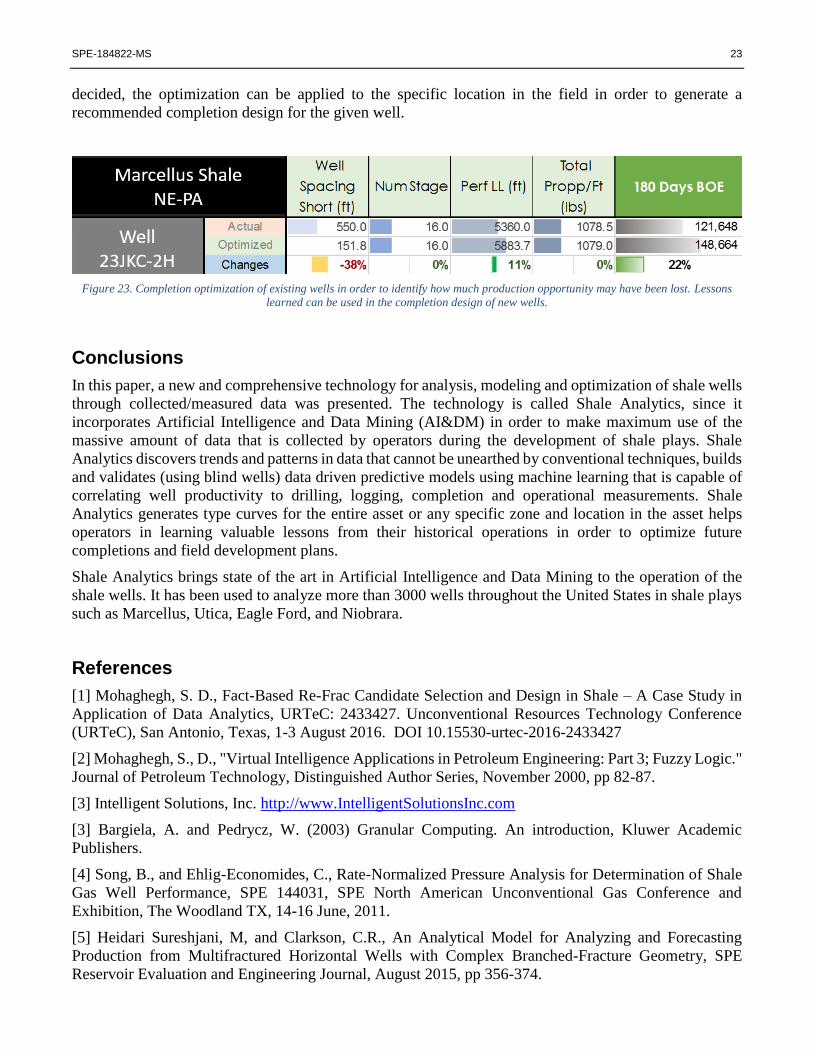
Completion Optimization Another use of the predictive model is to incorporate it into an evolutionary optimization routine for

completion optimization purposes. In this approach input parameters of the model that are associated with

the reservoir, characteristics are kept constant while the optimization routine looks for, and evolves the

most appropriate completion strategy for the given well. Figure 23 shows an example for a Marcellus

shale well in the Northeast of Pennsylvania. The predictive model for this asset that included more than

400 wells was developed in the same manner that was covered in this paper with some differences in the

parameters that were used to represent reservoir characteristics and completion and hydraulic fracture

design.

The operator of this particular asset was interested to learn from previous practices how “well spacing”

has impacted production, and if it can be optimized during the future development plans. Therefore, “well

spacing” data was made available and was incorporated in the model and later was used as an optimization

parameter. One of the lessons learned from this project was that, just like every other completion

parameter, there is no magic value of the well spacing that would be optimum everywhere in the field.

Given the heterogeneity of the shale and its natural fracture network that is very much responsible for well

productivity, wells in different locations of the field would have different optimum well spacing. As it is

clear from Figure 23, it was learned that the optimum well spacing for this particular well location is much

less than the value that was actually used. The Shale Analytics recommends a 38% reduction in well

spacing along with an 11% increase in lateral length in order to increase the well’s productivity by 22%.

This process is repeated for every well in the asset in order to learn the optimum manner in which this

asset can be developed. The asset is divided into zones and BTU areas. Therefore the optimization can be

conducted for each zone and each BTU area separately. Once the location of a particular well has been

SPE-184822-MS 23

decided, the optimization can be applied to the specific location in the field in order to generate a

recommended completion design for the given well.

Figure 23. Completion optimization of existing wells in order to identify how much production opportunity may have been lost. Lessons

learned can be used in the completion design of new wells.

Conclusions

In this paper, a new and comprehensive technology for analysis, modeling and optimization of shale wells

through collected/measured data was presented. The technology is called Shale Analytics, since it

incorporates Artificial Intelligence and Data Mining (AI&DM) in order to make maximum use of the

massive amount of data that is collected by operators during the development of shale plays. Shale

Analytics discovers trends and patterns in data that cannot be unearthed by conventional techniques, builds

and validates (using blind wells) data driven predictive models using machine learning that is capable of

correlating well productivity to drilling, logging, completion and operational measurements. Shale

Analytics generates type curves for the entire asset or any specific zone and location in the asset helps

operators in learning valuable lessons from their historical operations in order to optimize future

completions and field development plans.

Shale Analytics brings state of the art in Artificial Intelligence and Data Mining to the operation of the

shale wells. It has been used to analyze more than 3000 wells throughout the United States in shale plays

such as Marcellus, Utica, Eagle Ford, and Niobrara.

References

[1] Mohaghegh, S. D., Fact-Based Re-Frac Candidate Selection and Design in Shale – A Case Study in

Application of Data Analytics, URTeC: 2433427. Unconventional Resources Technology Conference

(URTeC), San Antonio, Texas, 1-3 August 2016. DOI 10.15530-urtec-2016-2433427

[2] Mohaghegh, S., D., "Virtual Intelligence Applications in Petroleum Engineering: Part 3; Fuzzy Logic."

Journal of Petroleum Technology, Distinguished Author Series, November 2000, pp 82-87.

[3] Intelligent Solutions, Inc. http://www.IntelligentSolutionsInc.com

[3] Bargiela, A. and Pedrycz, W. (2003) Granular Computing. An introduction, Kluwer Academic

Publishers.

[4] Song, B., and Ehlig-Economides, C., Rate-Normalized Pressure Analysis for Determination of Shale

Gas Well Performance, SPE 144031, SPE North American Unconventional Gas Conference and

Exhibition, The Woodland TX, 14-16 June, 2011.

[5] Heidari Sureshjani, M, and Clarkson, C.R., An Analytical Model for Analyzing and Forecasting

Production from Multifractured Horizontal Wells with Complex Branched-Fracture Geometry, SPE

Reservoir Evaluation and Engineering Journal, August 2015, pp 356-374.

24 SPE-184822-MS

[6] Clarkson, C.R., Qanbari, F., and Williams-Kovacs, J.D., Semi-Analytical Model for Matching

Flowback and Early-Time Production of Multi-Fractured Horizontal Tight Oil Wells, URTeC: 2460083,

Unconventional Resources Technology Conference, San Antonio, Texas, USA, 1-3 August 2016. DOI

10.15530-urtec-2016-2460083.

[7] Mohaghegh, S.D., Formation vs. Completion: Determining the Main Drivers behind Production from

Shale? A Case Study Using Data-Driven Analytics. URTeC 2147904, Unconventional Resources

Technology Conference. San Antonio, Texas, USA, 20-22 July 2015.