Spawning habitat rehabilitation – II. Using hypothesis

Intl. J. River Basin Management Vol. 2, No. 1 (2004), pp. 21–37

© 2004 IAHR & INBO

Spawning habitat rehabilitation – II. Using hypothesis development and testingin design, Mokelumne River, California, U.S.A.JOSEPH M. WHEATON, Department of Land, Air, and Water Resources, University of California at Davis,One Shields Avenue, Davis, CA 95616Corresponding Author: School of Geography, University of Southampton, Highfield, Southampton SO17 1BJE-mail: [email protected]

GREGORY B. PASTERNACK, Department of Land, Air, and Water Resources, University of California at Davis,One Shields Avenue, Davis, CA 95616

JOSEPH E. MERZ, East Bay Municipal Utility District, 1 Winemasters Way, Lodi, CA 95240; Department of Wildlife,Fish and Conservation Biology, University of California at Davis, One Shields Avenue, Davis, CA 95616

ABSTRACTRehabilitation of salmonid spawning habitat in regulated rivers through spawning bed enhancement is commonly used to mitigate altered sedimentand flow regimes and associated declines in salmonid communities. Partial design-phase predictive results are reported from the application of SHIRA(Spawning Habitat Integrated Rehabilitation Approach) on the lower Mokelumne River, California. The primary management goal of the projectwas to improve habitat for spawning and incubation life stages of fall-run chinook salmon (Oncorhynchus tshawytscha). In the summer of 2001, weconducted a pre-project appraisal followed by development and testing of 12 design scenarios. A subsample of eight design hypotheses, used in three ofthe design scenarios, is presented. Hydrodynamic, habitat suitability and sediment entrainment model results were used to test five of the eight designhypotheses. Two of the three hypotheses not tested were due to inadequate data on flow boundary conditions at high discharges. In September 2001, theproject was constructed in a 152 m reach of the LMR from a final design based on all eight of the design hypotheses presented. Transparent hypothesisdevelopment and testing in design is emphasized as opposed to declaring success or failure from an ongoing long-term monitoring campaign of thecase study presented.

Keywords: river restoration design; gravel augmentation; spawning gravels; habitat enhancement; Mokelumne River; fall-run chinooksalmon (Oncorhynchus tshawytscha).

1 Introduction

In the Central Valley of California, U.S.A., rivers thatonce sustained robust runs of chinook salmon (Oncorhynchustshawytscha) are now regulated or otherwise impacted by dams,diversions, chanelisation and instream gravel mining (Yoshiyamaet al., 1998). The decline of salmonids in regulated rivers hasbeen linked to many perturbations including over-harvest andthe deterioration, inaccessibility and reduction of spawning habi-tat for these fish (Maddock, 1999; Moyle and Randall, 1998;Nehlsen et al., 1991). In an inventory of gravel injection projectswithin California’s Central Valley from 1976 to 1999, Lutrickand Kondolf (p. comm.) identified 73 spawning habitat rehabil-itation (SHR) projects, on 19 different rivers, totalling over 45US$ million, and involving the addition of over 1.2 million m3

(1.8 million metric tons) of gravel. Wheaton et al. (2004) segre-gate SHR projects into three categories: (1) gravel augmentation,(2) hydraulic structure placement and (3) spawning bed enhance-ment. The two most dominant forms of SHR in California are

Received and accepted

21

gravel augmentation and spawning bed enhancement and mosthave not included a detailed design process but instead reliedon prescriptive treatments (Kondolf, 2000b). SHR as a type ofriver restoration is an indicator-species-centred endeavour thatfocuses on a specific ecological function connected to and indica-tive of other functions in an effort to promote broader ecosystemrecovery. Benefits to a diverse range of other ecological func-tions, dependent on hydrogeomorphic processes across a range ofspatiotemporal scales, are presumed to follow (Maddock, 1999).

Despite the popularity of SHR in practice, it has received littleattention in the peer-reviewed literature (Wheaton et al., 2004).Kondolf et al. (1996) reviewed a case study of a riffle construction(spawning bed enhancement) on the Merced River, California;and found geomorphic considerations to be lacking. Kondolf(2000b) offered suggestions for SHR, emphasizing the impor-tance of geomorphic assessment across multiple spatiotemporalscales. Merz and Setka (in press) outlined several techniques theyused to evaluate and monitor a spawning bed enhancement projectconstructed in 2000 on the Mokelumne River, California and

22 Joseph M. Wheaton et al.

implemented without a design approach. In a separate spawningbed enhancement project constructed in 1999 on the MokelumneRiver, California, Pasternack et al. (in press) established thatmore efficient use of gravel and spawning habitat could have beenachieved had 2D hydrodynamic and habitat suitability modelsbeen used to develop design alternatives. Measurement of habitatenhancement success has been variable with little work assessingdesign, implementation or longevity of projects. Despite numer-ous sources of uncertainty in the restoration process, which makedeveloping specific or appropriate performance measures diffi-cult, methods to cope with uncertainty in restoration are almostnon-existent in the literature.

In a companion paper (Wheaton et al., 2004) we reviewedthe application of a variety of existing science-based tools andconcepts to design and analyze SHR projects in regulated riversand suggested the SHIRA (Spawning Habitat Integrated Reha-bilitation Approach) framework to be employed with those tools.Ideally, the utility of this approach might be tested by monitoringfish populations at experimental rehabilitation sites. In practice,such trends are strongly influenced by many external factors andinternal intermediate mechanisms related to flow and sedimentdynamics, run-size and timing, changes in harvest regulations,and ocean harvesting and predation (Yoshiyama et al., 1998).Thus, comprehensive post project appraisal evaluating specificmechanistic links among hydrodynamics, geomorphology, andecology is an important aspect of river restoration (Downs andKondolf, 2002). This topic has been investigated repeatedly inthe peer reviewed literature, though the degree of practicalityimplementing post project appraisal remains uncertain.

Rather than providing the story of a rehabilitation projectthrough post project appraisal, the aim of this paper is to illustratethe utility of hypothesis development and testing during design.The river restoration literature is rich with case-by-case criticismbut lacks detailed SHR design advice for practitioners (Wilcock,1997). Traditional scientific hypothesis testing takes many forms(after Schumm, 1991):

• Falsification – trying to disprove a hypotheses (Popper, 1968)• Statistical Inference – deduce statistical hypotheses (H0 & HA)

and iteratively refine a scientific hypothesis based on inferenceand rejection of null hypothesis (Anderson, 1998)

• Ruling hypothesis – induction of a single hypothesis(Beveridge, 1980)

• Multiple working hypothesis (Chamberlin, 1890) – formulationof as many sequential, parallel or composite hypotheses aspossible (Schumm, 1991)

Design hypothesis testing, as presented here, differs from tradi-tional scientific hypothesis testing. The latter aims to universallycorroborate or disprove a tentative explanation based on observedevidence. In contrast, a design hypothesis is a mechanistic infer-ence, formulated on the basis of scientific literature review, andthus is assumed true as a general scientific principle. Hence,design hypothesis testing examines for presence of generallyaccepted functional or process attributes inherent in a designhypothesis in the specific, relevant setting. Design hypothesistesting does not test the overall validity of the scientific principle.

Design hypothesis falsification of a specific site design could be ahighly useful and cost-effective tool. Under some circumstances,such falsification may also provide insight and testing of underly-ing scientific principles that would be of great value to the largerscientific community as well (Cao and Carling, 2002). Selectedresults from the design phase of a spawning bed enhancementproject implemented with SHIRA on the lower MokelumneRiver, California are used as to demonstrate the utility of designhypothesis testing (see Wheaton, 2003 for details).

2 Study reach

The Mokelumne River of central California drains a 1700 km2

catchment westward to the Sacramento-San Joaquin Delta (seealso Merz, 2001a). Sixteen major dams or diversions, includingthe 0.24 km3 Pardee and the 0.51 km3 Camanche reservoirs, havedramatically altered the Lower Mokelumne River’s (LMR) flowregime (Pasternack et al., in press). A flood frequency analysisusing a Log Pearson III distribution reveals a dramatic reduc-tion in discharge after the construction of Pardee and CamancheReservoirs. The two, five, ten and one hundred year recurrenceinterval flows were reduced from pre Camanche dam levels by67%, 59%, 73% and 75% respectively. The fragmentation ofthe Mokelumne River basin via damming has completely alteredthe hydrology, and disconnected the flux of sediment from theupper basin to the LMR. Hence, spawning gravels have not beenreplenished from the upper basin since the construction of PardeeReservoir in 1929. Excluding enhancement, all sediment nowsupplied in the LMR is derived from erosion of existing relicdeposits, its own bed and fine-grained sediment primarily fromagricultural runoff. In basins like the Mokelumne where damremoval is not under consideration, SHR is a compromise toprovide some ecological function in a new downscaled systempositioned downstream of a major dam (Trush et al., 2000).

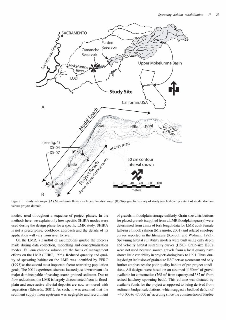
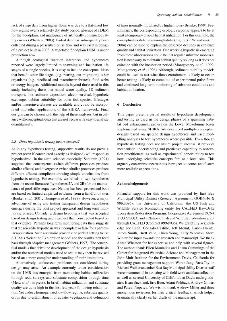
The LMR spans 72 km from the Delta to Camanche Dam,which has a chinook salmon and steelhead (O. mykiss) fish hatch-ery but no fish ladder (Figure 1A). The majority of salmonidspawning now takes place in a 14-km reach between CamancheDam and Elliot Road (Merz and Setka, in press). In addition tonative anadromous steelhead and fall-run chinook salmon, at least34 other fish species occur in the LMR (Merz, 2001a). Slopesthroughout the current spawning reaches are low (ranging from0.0005 to 0.002). The study reach begins 580 m downstreamof Camanche Dam and 76 m downstream of the confluence ofMurphy Creek (a 13.4 km2 subbasin). From June to July of 2001,the pre project phase was carried out within the 272 m long studyreach (Figure 1B). From early July to mid August the designphases detailed in this paper were conducted on 152 m reachcontained within the study reach.

3 Methods

3.1 Specific application of SHIRA to lower Mokelumne River

As detailed in the companion paper (Wheaton et al., 2004),SHIRA is organized into a set of science-based tools, termed

Spawning habitat rehabilitation – II 23

Proje

ct R

each

Model

Rea

ch

(focu

s of g

rave

l pla

cem

ent) 50 cm contour

interval shownglide

pool

pool poolriffle directionof flow

access road

California, USA

CamancheReservoir

PardeeReservoir

SACRAMENTO

Sacr

amen

to R

iver

Upper Mokelumne Basin

Study Site

MokelumneRiver

LODI

B

A

(see fig. 4)XS-04XS-07

0 20 40 60 80 100

meters

Figure 1 Study site maps. (A) Mokelumne River catchment location map. (B) Topographic survey of study reach showing extent of model domainversus project domain.

modes, used throughout a sequence of project phases. In themethods here, we explain only how specific SHIRA modes wereused during the design phase for a specific LMR study. SHIRAis not a prescriptive, cookbook approach and the details of itsapplication will vary from river to river.

On the LMR, a handful of assumptions guided the choicesmade during data collection, modelling and conceptualizationmodes. Fall-run chinook salmon are the focus of managementefforts on the LMR (FERC, 1998). Reduced quantity and qual-ity of spawning habitat on the LMR was identified by FERC(1993) as the second most important factor restricting populationgoals. The 2001 experiment site was located just downstream of amajor dam incapable of passing coarse-grained sediment. Due toflow reductions, the LMR is largely disconnected from its flood-plain and once-active alluvial deposits are now armoured withvegetation (Edwards, 2001). As such, it was assumed that thesediment supply from upstream was negligible and recruitment

of gravels in floodplain storage unlikely. Grain size distributionsfor placed gravels (supplied from a LMR floodplain quarry) weredetermined from a mix of fork length data for LMR adult femalefall-run chinook salmon (Miyamoto, 2001) and related envelopecurves reported in the literature (Kondolf and Wolman, 1993).Spawning habitat suitability models were built using only depthand velocity habitat suitability curves (HSC). Grain-size HSCswere not used because source gravels from a local quarry haveshown little variability in projects dating back to 1991. Thus, dur-ing design inclusion of grain-size HSC acts as a constant and onlyfurther emphasizes the poor quality habitat of pre-project condi-tions. All designs were based on an assumed 1150 m3 of gravelavailable for construction (768 m3 from a quarry and 382 m3 fromretired hatchery spawning beds). This volume was dictated byavailable funds for the project as opposed to being derived fromsediment budget calculations, which suggest a bedload deficit of∼40,000 to 47, 000 m3 accruing since the construction of Pardee


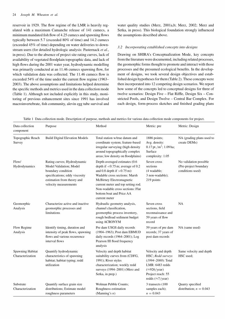
reservoir in 1929. The flow regime of the LMR is heavily reg-ulated with a maximum Camanche release of 141 cumecs, aminimum mandated fish flow of 4.25 cumecs and spawning flowstypically between 5.7 (exceeded 80% of time) and 14.2 cumecs(exceeded 45% of time) depending on water deliveries to down-stream users (for detailed hydrologic analysis: Pasternack et al.,in press). Due to the absence of project site rating curves, lack ofavailability of vegetated floodplain topographic data, and lack ofhigh flows during the 2001 water year, hydrodynamic modellingwas primarily conducted at an 11.46 cumecs spawning flow, forwhich validation data was collected. The 11.46 cumecs flow isexceeded 54% of the time under the current flow regime (1963–2003). The above assumptions and limitations helped determinethe specific methods and metrics used in the data collection mode(Table 1). Although not included explicitly in this study, moni-toring of previous enhancement sites since 1991 has involvedmacroinvertebrate, fish community, alevin egg tube survival and

Table 1 Data collection mode. Description of purpose, methods and metrics for various data collection mode components for project.

Data collectioncomponent

Purpose Method Metric: pre Metric: Design

Topographic ReachSurvey

Build Digital Elevation Models Total station w/true datum andcoordinate system; feature-basedirregular surveying (high densityaround topographically complexareas; low density on floodplains)

1886 points;Avg. density:0.17 pt./m2; 1.09 ha;Surfacecomplexity: 1.05

NA (grading plans used tocreate DEMs)

Flow/Hydrodynamics

Rating curves; HydrodynamicModel Validation; Modelboundary conditionspecifications; eddy viscosityestimation from theory andvelocity measurements

Depth-averaged estimates (0.6depth if <0.75 m; average of 0.2and 0.8 depth if >0.75 m):Wadable cross sections: MarshMcBirney Electromagneticcurrent meter and top setting rod.Non-wadable cross sections: Flatbottom boat and Price AAcurrent meter

Seven crosssections(4 wadable;3 non-wadable);219 points

No validation possible(Pre-project boundaryconditions used)

GeomorphicAnalysis

Characterize active and inactivegeomorphic processes andlimitations

Hydraulic geometry analysis,channel classification,geomorphic process inventory,rough bedload sediment budgetusing ACRONYM

Seven crosssections, fieldreconnaissance and59 years of flowrecord

NA

Flow RegimeAnalysis

Identify timing, duration andintensity of peak flows, spawningflows and various recurrenceinterval flows

Pre dam USGS daily records(1904–1963); Post dam EBMUDdaily records (1964–2001); LogPearson III flood frequencyanalysis

59 years of pre damrecords; 37 years ofpost dam records

NA (same used)

Spawning HabitatCharacterization

Quantify hydrodynamiccharacteristics of spawninghabitat; habitat typing; reddutilization

Velocity and depth habitatsuitability curves from (CDFG,1991); River stylescharacterization; weekly reddsurveys (1994–2001) (Merz andSetka, in prep.)

Velocity and depthHSC; Redd surveys(1994–2000): TotalLMR: 6483 redds(≈926/year)Project reach: 55redds (≈7/year)

Same velocity and depthHSC used;

SubstrateCharacterization

Quantify surface grain sizedistributions; Estimate modelroughness parameters

Wolman Pebble Counts;Roughness estimation(Manning’s n)

3 transects (100samples each);n = 0.043

Quarry specifieddistribution; n = 0.043

water quality studies (Merz, 2001a,b; Merz, 2002; Merz andSetka, in press). This biological foundation strongly influencedthe assumptions described above.

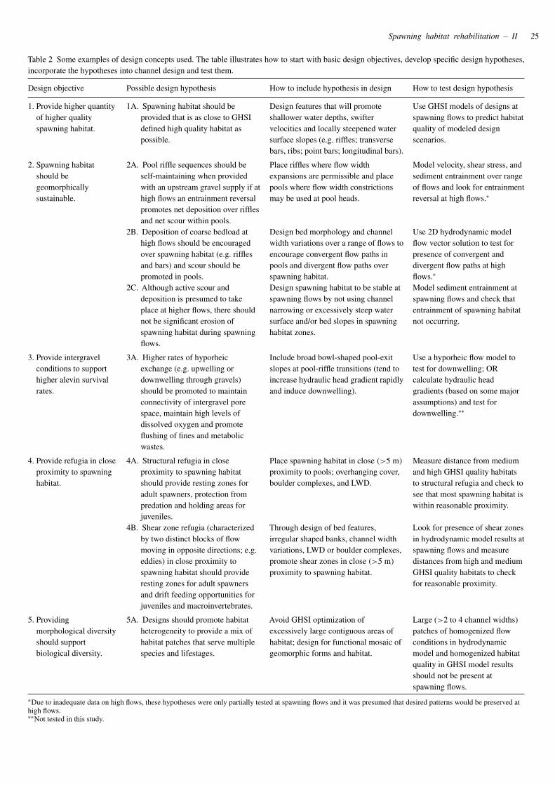
3.2 Incorporating established concepts into designs

Drawing on SHIRA’s Conceptualization Mode, key conceptsfrom the literature were documented, including related processes,the geomorphic forms thought to promote and interact with thoseprocesses and the presumed ecological benefits. In the develop-ment of designs, we took several design objectives and estab-lished design hypotheses for them (Table 2). These concepts werethen incorporated into 12 competing design scenarios. We reporthow some of the concepts led to conceptual designs for three oftwelve scenarios: Design Five – Flat Riffle, Design Six – Con-stricted Pools, and Design Twelve – Central Bar Complex. Foreach design, form-process sketches and finished grading plans


Table 2 Some examples of design concepts used. The table illustrates how to start with basic design objectives, develop specific design hypotheses,incorporate the hypotheses into channel design and test them.

Design objective Possible design hypothesis How to include hypothesis in design How to test design hypothesis

1. Provide higher quantityof higher qualityspawning habitat.

1A. Spawning habitat should beprovided that is as close to GHSIdefined high quality habitat aspossible.

Design features that will promoteshallower water depths, swiftervelocities and locally steepened watersurface slopes (e.g. riffles; transversebars, ribs; point bars; longitudinal bars).

Use GHSI models of designs atspawning flows to predict habitatquality of modeled designscenarios.

2. Spawning habitatshould begeomorphicallysustainable.

2A. Pool riffle sequences should beself-maintaining when providedwith an upstream gravel supply if athigh flows an entrainment reversalpromotes net deposition over rifflesand net scour within pools.

Place riffles where flow widthexpansions are permissible and placepools where flow width constrictionsmay be used at pool heads.

Model velocity, shear stress, andsediment entrainment over rangeof flows and look for entrainmentreversal at high flows.∗

2B. Deposition of coarse bedload athigh flows should be encouragedover spawning habitat (e.g. rifflesand bars) and scour should bepromoted in pools.

Design bed morphology and channelwidth variations over a range of flows toencourage convergent flow paths inpools and divergent flow paths overspawning habitat.

Use 2D hydrodynamic modelflow vector solution to test forpresence of convergent anddivergent flow paths at highflows.∗

2C. Although active scour anddeposition is presumed to takeplace at higher flows, there shouldnot be significant erosion ofspawning habitat during spawningflows.

Design spawning habitat to be stable atspawning flows by not using channelnarrowing or excessively steep watersurface and/or bed slopes in spawninghabitat zones.

Model sediment entrainment atspawning flows and check thatentrainment of spawning habitatnot occurring.

3. Provide intergravelconditions to supporthigher alevin survivalrates.

3A. Higher rates of hyporheicexchange (e.g. upwelling ordownwelling through gravels)should be promoted to maintainconnectivity of intergravel porespace, maintain high levels ofdissolved oxygen and promoteflushing of fines and metabolicwastes.

Include broad bowl-shaped pool-exitslopes at pool-riffle transitions (tend toincrease hydraulic head gradient rapidlyand induce downwelling).

Use a hyporheic flow model totest for downwelling; ORcalculate hydraulic headgradients (based on some majorassumptions) and test fordownwelling.∗∗

4. Provide refugia in closeproximity to spawninghabitat.

4A. Structural refugia in closeproximity to spawning habitatshould provide resting zones foradult spawners, protection frompredation and holding areas forjuveniles.

Place spawning habitat in close (>5 m)

proximity to pools; overhanging cover,boulder complexes, and LWD.

Measure distance from mediumand high GHSI quality habitatsto structural refugia and check tosee that most spawning habitat iswithin reasonable proximity.

4B. Shear zone refugia (characterizedby two distinct blocks of flowmoving in opposite directions; e.g.eddies) in close proximity tospawning habitat should provideresting zones for adult spawnersand drift feeding opportunities forjuveniles and macroinvertebrates.

Through design of bed features,irregular shaped banks, channel widthvariations, LWD or boulder complexes,promote shear zones in close (>5 m)

proximity to spawning habitat.

Look for presence of shear zonesin hydrodynamic model results atspawning flows and measuredistances from high and mediumGHSI quality habitats to checkfor reasonable proximity.

5. Providingmorphological diversityshould supportbiological diversity.

5A. Designs should promote habitatheterogeneity to provide a mix ofhabitat patches that serve multiplespecies and lifestages.

Avoid GHSI optimization ofexcessively large contiguous areas ofhabitat; design for functional mosaic ofgeomorphic forms and habitat.

Large (>2 to 4 channel widths)patches of homogenized flowconditions in hydrodynamicmodel and homogenized habitatquality in GHSI model resultsshould not be present atspawning flows.

∗Due to inadequate data on high flows, these hypotheses were only partially tested at spawning flows and it was presumed that desired patterns would be preserved athigh flows.∗∗Not tested in this study.


depict the utility of SHIRA’s conceptualization mode at creativelyincorporating scientific concepts into designs (Wheaton, 2003).

Finished grading plans were drawn in AutoCAD andTIN-based digital elevation models (DEMs) were created inAutoDesk’s Land Desktop R3. A finished grading plan speci-fies finished grade elevations in reference to a pre-project DEM.A pre-project DEM was made from detailed topographic surveys.Design DEMs combined the pre-project DEM with grading plansfor hypothetical designs (Table 1). DEMs were each iterativelydeveloped using (1) visualization, (2) editing, (3) data augmen-tation and (4) interpolation stages. Point data augmentation wasused to improve pre-project DEM representation of areas withlower point resolution or inadequate data (typically deep pools).Three types of point augmentation were used: (1) additional fieldsurveys, (2) interpolation between known points and (3) user-specified spacing along contours. When iterative DEM develop-ment finally yielded realistic terrain representation, refined pointand breakline data were extrapolated from Land Desktop for lateruse in hydrodynamic model mesh characterization.

3.3 Numerical models for process predictions

SHIRA’s Modelling Mode was used to create hydrodynamic, sed-iment entrainment and spawning habitat models that in turn wereused to test specific design hypotheses (Table 2). Model resultsare presented for the pre-project (for validation and comparison)and three design scenarios. Emphasis is placed on the abilityor inability of these models to test the design hypotheses made.The models used are reviewed briefly below (see also Pasternacket al., in press).

The 2D Finite Element Surface Water Modelling System(FESWMS) and Surfacewater Modelling System graphical inter-face were used to analyze steady state hydrodynamics. Theboundary conditions required to run FESWMS are: (1) a dis-charge at the upstream boundary, (2) a corresponding watersurface elevation at the downstream boundary and (3) channeltopography. Due to inadequate flow variation during the 2001water year, lack of forested floodplain topographic data, andlack of historical rating curves for the reach, discharge and watersurface boundary conditions were identified only for spawningflows (11.46 cumecs). Refined DEM data were used to discretizechannel topography to a finite element model mesh at an approx-imately uniform node spacing (∼45 cm apart). This resulted inmodel meshes with between 49,000 and 53,000 computationalnodes comprising between 15,000 and 16,500 quadrilateral andtriangular elements. The most noteworthy model parametersinclude Manning’s roughness and Boussinesq’s eddy viscositycoefficient for turbulence closure. Manning’s roughness (n) wasestimated as 0.043 for entire study site using a McCuen summa-tion method (McCuen, 1989). This was used instead of a spatiallyexplicit application of Strickler’s equation for roughness basedon substrate size variations, because in this instance there was anarrow and homogenized range of gravel substrate sizes. Eddyviscosity is a fourth-order tensor (33 terms), which describes theproperty of the flow and arises from the closure problem whenaveraging the velocity terms in the Navier-Stokes equations. We

used Boussinesq’s analogy to parameterize eddy viscosity, whichcrudely approximates eddy viscosity as an isotropic scalar. Doingso allows a theoretical estimate of eddy viscosity as 60 percent ofthe product of shear-velocity (u*) and depth (Froehlich, 1989).Pasternack et al. (in press) were unable to achieve model stabilityfor a reach with a shallow riffle and a relatively deep, in-channelmining pit using a single constant eddy viscosity value estimatedfrom field measured depth and velocity data with a mesh builton unrefined DEM data at a study site located 220 m upstream.In fact, model stability was only achieved when the constanteddy viscosity was kept above 0.065 m2/sec. During a flow of11.46 cumecs at the study site reported here, an average eddyviscosity of 0.017 m2/sec was calculated from 219 velocity anddepth measurements. Due to significantly less topographic vari-ation as well as higher mesh and DEM quality in this study,model stability and convergence was achieved even using theactual calculated eddy viscosity value of 0.017 m2/sec. No modelcalibration was performed as all model parameters were speci-fied with actual measured or theoretically calculated values. Preproject model results (velocity and depth) were compared againstmeasured values at five cross sections for validation.

Habitat suitability curves for fall-run chinook on the LMRwere used to develop a global habitat suitability index (GHSI)for spawning (Wheaton et al., 2004). In principle, this is similarto PHABSIM habitat simulations with the major exception thata 2D instead of 1D hydrodynamic model is used (Leclerc et al.,1995). The index yields spatial predictions of spawning habitatsuitability based on 2D hydrodynamic model results (Pasternacket al., in press). Whereas the hydrodynamic model results can beused to test specific hydrodynamic process predictions and makeecological function inferences, the habitat suitability model teststhe claim that specific forms will produce preferable spawninghabitat conditions.

A sediment entrainment sub-model based on hydrodynamicmodel results and representative grain sizes (d16, d50 and d84)

was used to test for potential scour at spawning flows. A com-mon approach to modelling sediment entrainment using Shields’incipient motion criterion (Garde and Raju, 1985), and Einstein’slog velocity profile equation was employed (Wheaton et al.,2004). The theoretical HSC and entrainment functions were ana-lyzed by plotting them as a third dimension on velocity versusdepth plots. Actual measured hydraulic conditions (velocity anddepth) could then be overlaid on the same plot to assess both habi-tat suitability and sediment entrainment thresholds. Sedimententrainment model results were used to test for erosion at lowspawning flows, but could not be used to test hypothesized ero-sion processes at higher flows due to lack of adequate rating curvedata coupled with an un-surveyed, wide, and complex vegetatedfloodplain.

4 Results

4.1 Incorporating established concepts into designs

The pre-project topographic survey and geomorphic habitatclassification revealed a pre-project reach-averaged slope of


Table 3 Summary grading statistics.

Design Volume Gravel Maximum Bed elevation Localof gravel placement fill depth at riffle slopeused footprint (m) crest(m3) (m2) (m)

Pre NA NA NA 26.90 0.0011Five 961 2225 1.5 27.66 0.0080Six 956 2457 1.4 27.51 0.0049Twelve 1146 2402 1.5 27.44* 0.0020

*Upper riffle reported (central bar raised from 27.02 to 27.75 and lower riffleraised from 26.66 m to 27.44 m).

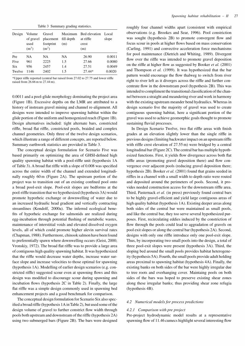
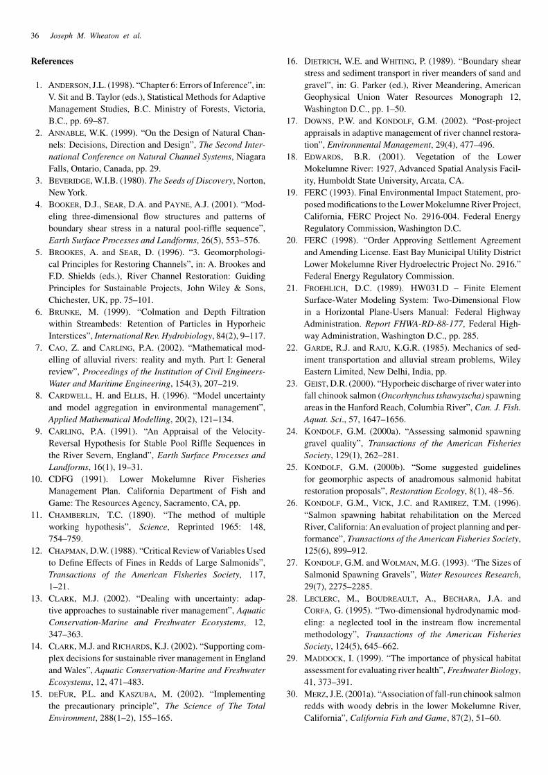
0.0011 and a pool-glide morphology dominating the project area(Figure 1B). Excessive depths on the LMR are attributed to ahistory of instream gravel mining and channel re-alignment. Alldesigns were intended to improve spawning habitat within theglide portion of the uniform and homogenized reach (Figure 1B).Design alternatives included: tight alternate bars, constrictedriffle, broad flat riffle, constricted pools, braided and complexchannel geometries. Only three of the twelve design scenarios,which illustrate a range of different concepts, are reported below.Summary earthwork statistics are provided in Table 3.

The conceptual design formulation for Scenario Five wasbased primarily on optimizing the area of GHSI-defined highquality spawning habitat with a pool-riffle unit (hypothesis 1Aof Table 3). A broad flat riffle with a slope of 0.008 was specifiedacross the entire width of the channel and extended longitudi-nally roughly 60 m (Figure 2A). The upstream portion of theproject was to transition out of an existing confined pool ontoa broad pool-exit slope. Pool-exit slopes are bedforms at thepool-riffle transition that we hypothesized (hypothesis 3A) wouldpromote hyporheic exchange or downwelling of water due toan increased hydraulic head gradient and vertically contractingstreamlines (Kondolf, 2000a). The inferred ecological bene-fits of hyporheic exchange for salmonids are realized duringegg-incubation through potential flushing of metabolic wastes,maintenance of interstitial voids and elevated dissolved oxygenlevels, all of which could promote higher alevin survival rates(Chapman, 1988). Furthermore, chinook salmon have been foundto preferentially spawn where downwelling occurs (Geist, 2000;Vronskiy, 1972). The broad flat riffle was to provide a large areaof contiguous high quality spawning habitat. It was hypothesizedthat the riffle would decrease water depths, increase water sur-face slope and increase velocities to those optimal for spawning(hypothesis 1A). Modelling of earlier design scenarios (e.g. con-stricted riffle) suggested scour even at spawning flows and thisdesign was modified to discourage scour during spawning andincubation flows (hypothesis 2C in Table 2). Finally, the largeflat riffle was a simple design commonly used in spawning bedenhancement projects and a good benchmark for comparison.

The conceptual design formulation for Scenario Six also spec-ified a broad riffle (hypothesis 1A in Table 2), but used some of thedesign volume of gravel to further constrict flow width throughpools both upstream and downstream of the riffle (hypothesis 2A)using two submerged bars (Figure 2B). The bars were designed

roughly four channel widths apart (consistent with empiricalobservations (e.g. Brookes and Sear, 1996). Pool constrictionwas sought (hypothesis 2B) to promote convergent flow andfocus scour in pools at higher flows based on mass conservation(Carling, 1991) and convective acceleration force mechanismsfor pool maintenance (Dietrich and Whiting, 1989). Divergentflow over the riffle was intended to promote gravel depositionon the riffle at higher flow as suggested by Booker et al. (2001)and Thompson et al. (1999). It was hypothesized that the barpattern would encourage the flow thalweg to switch from riverright to river left as it diverges across the riffle and further con-centrate flow in the downstream pool (hypothesis 2B). This wasintended to compliment the transitional classification of the chan-nel between a straight and meandering river and work in harmonywith the existing upstream meander bend hydraulics. Whereas indesign scenario five the majority of gravel was used to createcontiguous spawning habitat, here a significant portion of thegravel was used to achieve geomorphic goals thought to promotesustaining fluvial processes.

In Design Scenario Twelve, two flat riffle areas with finishgrades at an elevation slightly lower than the single riffle inprevious designs (limiting backwater impact on an upstream rifflewith riffle crest elevation of 27.55 m) were bridged by a centrallongitudinal bar (Figure 2C). The central bar has multiple hypoth-esized functions. First, it yields flow divergence across both flatriffle areas (promoting gravel deposition there) and flow con-vergence over adjacent pools (reducing gravel deposition there;hypothesis 2B). Booker et al. (2001) found that grains seeded inriffles in a channel with a small width to depth ratio were routedand deposited around the perimeters of pools. Second, it pro-vides needed construction access for the downstream riffle area.Third, Pasternack et al. (in press) previously found central barsto be highly gravel-efficient and yield large contiguous areas ofhigh quality habitat (hypothesis 1A). Existing deeper areas alongboth sides of the central bar were maintained as small pools,and like the central bar, they too serve several hypothesized pur-poses. First, recirculating eddies induced by the constriction offlow through the pools could lead to aggradation of gravels onpool exit slopes or along the central bar (hypothesis 2A). Second,designs with only one riffle introduce only one pool-exit slope.Thus, by incorporating two small pools into the design, a total ofthree pool-exit slopes were present (hypothesis 3A). Third, thesloping bed around the small pools provides habitat heterogene-ity (hypothesis 5A). Fourth, the small pools provide adult holdingareas proximal to spawning habitat (hypothesis 4A). Finally, theexisting banks on both sides of the bar were highly irregular dueto tree roots and overhanging cover. Maintaing pools on bothsides of the bars was hoped to preserve existing shear zonesalong these irregular banks; thus providing shear zone refugia(hypothesis 4B).

4.2 Numerical models for process predictions

4.2.1 Comparison with pre projectPre-project hydrodynamic model results at a representativespawning flow of 11.46 cumecs highlight several interesting flow


A

B

C0 20 40 60 80 100

meters

0-25 cm fill25-50 cm fill50-75 cm fill75-100 cm fill100-125 cm fill125-150 cm fill150-175 cm fill

lower riffle

central bar upper riffle

pool exit slopes

riffle

bar

bar

Figure 2 Conceptual designs and grading plans for selected design scenarios. (A) Design scenario 5 (flat riffle). (B) Design scenario 6 (constrictedpools). (C) Design scenario 12 (final design – complex channel geometry). Shaded areas represent depth of design specified gravel placement; whereasfaded contours represent pre project topography.

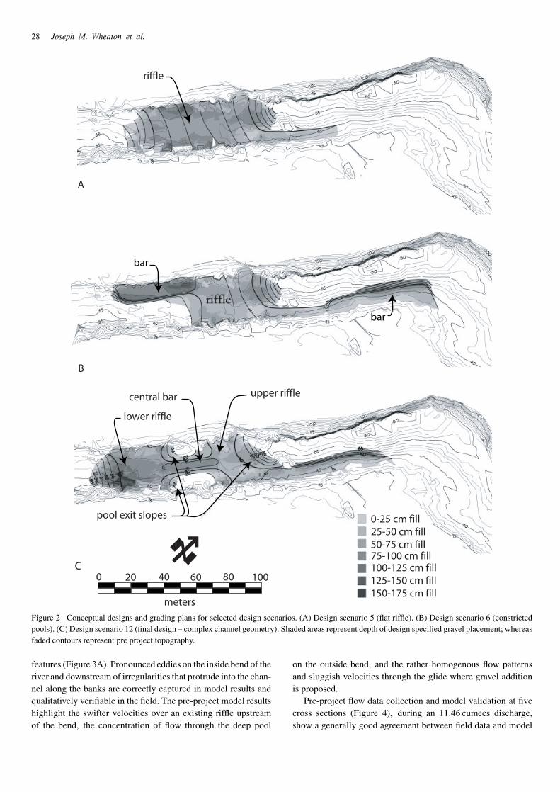
features (Figure 3A). Pronounced eddies on the inside bend of theriver and downstream of irregularities that protrude into the chan-nel along the banks are correctly captured in model results andqualitatively verifiable in the field. The pre-project model resultshighlight the swifter velocities over an existing riffle upstreamof the bend, the concentration of flow through the deep pool

on the outside bend, and the rather homogenous flow patternsand sluggish velocities through the glide where gravel additionis proposed.

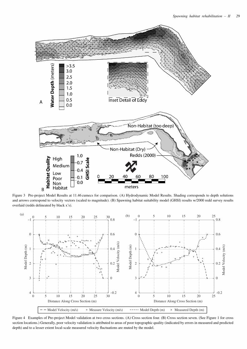
Pre-project flow data collection and model validation at fivecross sections (Figure 4), during an 11.46 cumecs discharge,show a generally good agreement between field data and model


Figure 3 Pre-project Model Results at 11.46 cumecs for comparison. (A) Hydrodynamic Model Results. Shading corresponds to depth solutionsand arrows correspond to velocity vectors (scaled to magnitude). (B) Spawning habitat suitability model (GHSI) results w/2000 redd survey resultsoverlaid (redds delineated by black x’s).

(a) (b)–1

0

1

2

3

4 –0.2

0

0.2

0.4

0.6

0.8

0 5 10 15 20 25 30

0 5 10 15 20 25 30

Mod

el D

epth

(m

)

Mod

el V

eloc

ity

(m/s

)

–1

0

1

2

3

4 –0.2

0

0.2

0.4

0.6

0.8

0 5 10 15 20 25

Model Depth (m) Measured Depth (m)Model Velocity (m/s) Measure Velocity (m/s)

0 5 10 15 20 25

Mod

el D

epth

(m

)

Mod

el V

eloc

ity

(m/s

)

Distance Along Cross Section (m)Distance Along Cross Section (m)

Figure 4 Examples of Pre-project Model validation at two cross sections. (A) Cross section four. (B) Cross section seven. (See Figure 1 for crosssection locations.) Generally, poor velocity validation is attributed to areas of poor topographic quality (indicated by errors in measured and predicteddepth) and to a lesser extent local-scale measured velocity fluctuations are muted by the model.


predictions (see Wheaton 2003 for full results). The largest errorsin velocity predictions are where model bathymetry inaccuratelydescribes the bed. The use of an intermediate AutoCAD-drivenDEM process in this study represented a significant advance inmodel prediction compared to an earlier study (Pasternack et al.,

A

B

C

Figure 5 Design Phase Hydrodynamic Model Results at 11.46 cumecs. Shading corresponds to depth solutions and arrows correspond to velocityvectors (scaled to magnitude). (A) Design scenario 5 (flat riffle). (B) Design scenario 6 (constricted pools). (C) Design scenario 12 (final design –complex channel geometry).

in press) in which raw survey data were directly interpolated toyield the model mesh.

For comparison, pre-project GHSI modelling results confirmthe lack of substantial areas of high or medium quality spawn-ing habitat within the proposed enhancement area (Figure 3B).


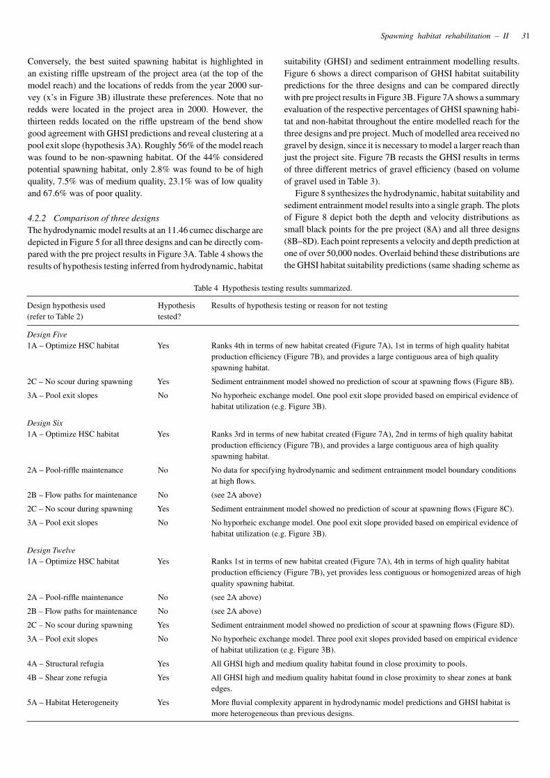
Conversely, the best suited spawning habitat is highlighted inan existing riffle upstream of the project area (at the top of themodel reach) and the locations of redds from the year 2000 sur-vey (x’s in Figure 3B) illustrate these preferences. Note that noredds were located in the project area in 2000. However, thethirteen redds located on the riffle upstream of the bend showgood agreement with GHSI predictions and reveal clustering at apool exit slope (hypothesis 3A). Roughly 56% of the model reachwas found to be non-spawning habitat. Of the 44% consideredpotential spawning habitat, only 2.8% was found to be of highquality, 7.5% was of medium quality, 23.1% was of low qualityand 67.6% was of poor quality.

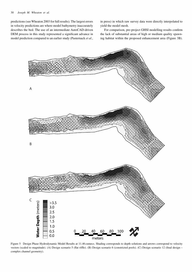
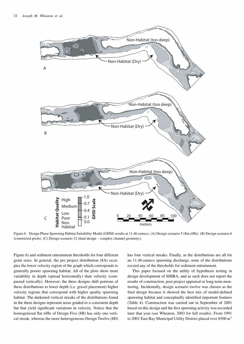
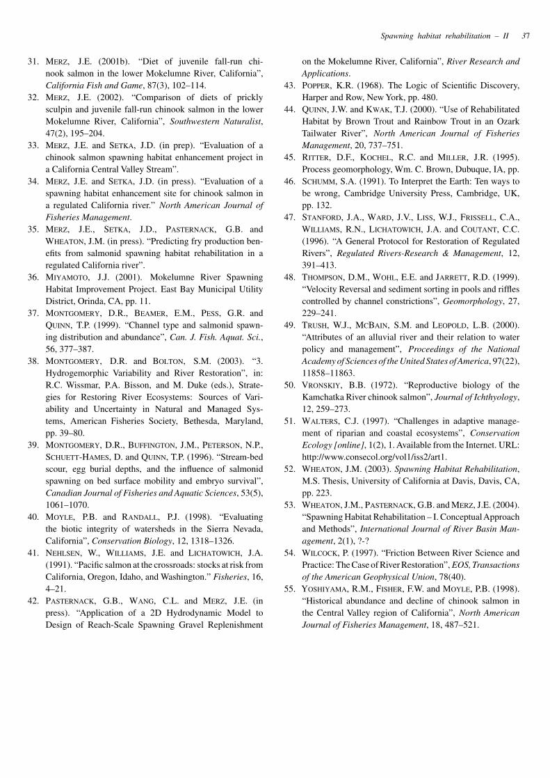
4.2.2 Comparison of three designsThe hydrodynamic model results at an 11.46 cumec discharge aredepicted in Figure 5 for all three designs and can be directly com-pared with the pre project results in Figure 3A. Table 4 shows theresults of hypothesis testing inferred from hydrodynamic, habitat

Table 4 Hypothesis testing results summarized.

Design hypothesis used(refer to Table 2)

Hypothesistested?

Results of hypothesis testing or reason for not testing

Design Five1A – Optimize HSC habitat Yes Ranks 4th in terms of new habitat created (Figure 7A), 1st in terms of high quality habitat

production efficiency (Figure 7B), and provides a large contiguous area of high qualityspawning habitat.

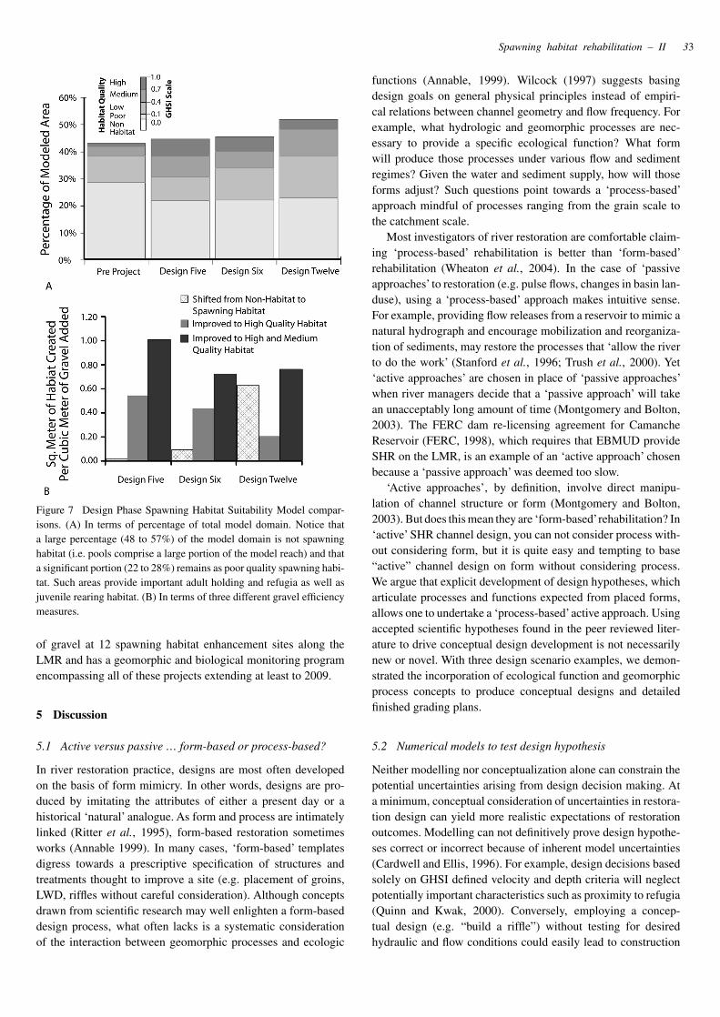
2C – No scour during spawning Yes Sediment entrainment model showed no prediction of scour at spawning flows (Figure 8B).

3A – Pool exit slopes No No hyporheic exchange model. One pool exit slope provided based on empirical evidence ofhabitat utilization (e.g. Figure 3B).

Design Six1A – Optimize HSC habitat Yes Ranks 3rd in terms of new habitat created (Figure 7A), 2nd in terms of high quality habitat

production efficiency (Figure 7B), and provides a large contiguous area of high qualityspawning habitat.

2A – Pool-riffle maintenance No No data for specifying hydrodynamic and sediment entrainment model boundary conditionsat high flows.

2B – Flow paths for maintenance No (see 2A above)

2C – No scour during spawning Yes Sediment entrainment model showed no prediction of scour at spawning flows (Figure 8C).

3A – Pool exit slopes No No hyporheic exchange model. One pool exit slope provided based on empirical evidence ofhabitat utilization (e.g. Figure 3B).

Design Twelve1A – Optimize HSC habitat Yes Ranks 1st in terms of new habitat created (Figure 7A), 4th in terms of high quality habitat

production efficiency (Figure 7B), yet provides less contiguous or homogenized areas of highquality spawning habitat.

2A – Pool-riffle maintenance No (see 2A above)

2B – Flow paths for maintenance No (see 2A above)

2C – No scour during spawning Yes Sediment entrainment model showed no prediction of scour at spawning flows (Figure 8D).

3A – Pool exit slopes No No hyporheic exchange model. Three pool exit slopes provided based on empirical evidenceof habitat utilization (e.g. Figure 3B).

4A – Structural refugia Yes All GHSI high and medium quality habitat found in close proximity to pools.

4B – Shear zone refugia Yes All GHSI high and medium quality habitat found in close proximity to shear zones at bankedges.

5A – Habitat Heterogeneity Yes More fluvial complexity apparent in hydrodynamic model predictions and GHSI habitat ismore heterogeneous than previous designs.

suitability (GHSI) and sediment entrainment modelling results.Figure 6 shows a direct comparison of GHSI habitat suitabilitypredictions for the three designs and can be compared directlywith pre project results in Figure 3B. Figure 7A shows a summaryevaluation of the respective percentages of GHSI spawning habi-tat and non-habitat throughout the entire modelled reach for thethree designs and pre project. Much of modelled area received nogravel by design, since it is necessary to model a larger reach thanjust the project site. Figure 7B recasts the GHSI results in termsof three different metrics of gravel efficiency (based on volumeof gravel used in Table 3).

Figure 8 synthesizes the hydrodynamic, habitat suitability andsediment entrainment model results into a single graph. The plotsof Figure 8 depict both the depth and velocity distributions assmall black points for the pre project (8A) and all three designs(8B–8D). Each point represents a velocity and depth prediction atone of over 50,000 nodes. Overlaid behind these distributions arethe GHSI habitat suitability predictions (same shading scheme as


High

Medium

Low

Non Habitat

Poor

Hab

itat

Qu

alit

y 1.0

0.7

0.4

0.10.0

GH

SI S

cale

A

C

B

Non-Habitat (too deep)

Non-Habitat (Dry)



0 20 40 60 80 100

meters

Non-Habitat (Dry)

Non-Habitat (Dry)

Figure 6 Design Phase Spawning Habitat Suitability Model (GHSI) results at 11.46 cumecs. (A) Design scenario 5 (flat riffle). (B) Design scenario 6(constricted pools). (C) Design scenario 12 (final design – complex channel geometry).

Figure 6) and sediment entrainment thresholds for four differentgrain sizes. In general, the pre project distribution (8A) occu-pies the lower velocity region of the graph which corresponds togenerally poorer spawning habitat. All of the plots show morevariability in depth (spread horizontally) than velocity (com-pacted vertically). However, the three designs shift portions ofthese distributions to lower depth (i.e. gravel placement) highervelocity regions that correspond with higher quality spawninghabitat. The darkened vertical streaks of the distributions foundin the three designs represent areas graded to a consistent depthbut that yield significant variations in velocity. Notice that thehomogenized flat riffle of Design Five (8B) has only one verti-cal streak, whereas the more heterogeneous Design Twelve (8D)

has four vertical streaks. Finally, as the distributions are all foran 11.46 cumecs spawning discharge, none of the distributionsexceed any of the thresholds for sediment entrainment.

This paper focused on the utility of hypothesis testing indesign development of SHIRA, and as such does not report theresults of construction, post project appraisal or long-term mon-itoring. Incidentally, design scenario twelve was chosen as thefinal design because it showed the best mix of model-definedspawning habitat and conceptually identified important features(Table 4). Construction was carried out in September of 2001based on this design and the first spawning activity was recordedlater that year (see Wheaton, 2003 for full results). From 1991to 2001 East Bay Municipal Utility District placed over 8500 m3


Figure 7 Design Phase Spawning Habitat Suitability Model compar-isons. (A) In terms of percentage of total model domain. Notice thata large percentage (48 to 57%) of the model domain is not spawninghabitat (i.e. pools comprise a large portion of the model reach) and thata significant portion (22 to 28%) remains as poor quality spawning habi-tat. Such areas provide important adult holding and refugia as well asjuvenile rearing habitat. (B) In terms of three different gravel efficiencymeasures.

of gravel at 12 spawning habitat enhancement sites along theLMR and has a geomorphic and biological monitoring programencompassing all of these projects extending at least to 2009.

5 Discussion

5.1 Active versus passive … form-based or process-based?

In river restoration practice, designs are most often developedon the basis of form mimicry. In other words, designs are pro-duced by imitating the attributes of either a present day or ahistorical ‘natural’ analogue. As form and process are intimatelylinked (Ritter et al., 1995), form-based restoration sometimesworks (Annable 1999). In many cases, ‘form-based’ templatesdigress towards a prescriptive specification of structures andtreatments thought to improve a site (e.g. placement of groins,LWD, riffles without careful consideration). Although conceptsdrawn from scientific research may well enlighten a form-baseddesign process, what often lacks is a systematic considerationof the interaction between geomorphic processes and ecologic

functions (Annable, 1999). Wilcock (1997) suggests basingdesign goals on general physical principles instead of empiri-cal relations between channel geometry and flow frequency. Forexample, what hydrologic and geomorphic processes are nec-essary to provide a specific ecological function? What formwill produce those processes under various flow and sedimentregimes? Given the water and sediment supply, how will thoseforms adjust? Such questions point towards a ‘process-based’approach mindful of processes ranging from the grain scale tothe catchment scale.

Most investigators of river restoration are comfortable claim-ing ‘process-based’ rehabilitation is better than ‘form-based’rehabilitation (Wheaton et al., 2004). In the case of ‘passiveapproaches’ to restoration (e.g. pulse flows, changes in basin lan-duse), using a ‘process-based’ approach makes intuitive sense.For example, providing flow releases from a reservoir to mimic anatural hydrograph and encourage mobilization and reorganiza-tion of sediments, may restore the processes that ‘allow the riverto do the work’ (Stanford et al., 1996; Trush et al., 2000). Yet‘active approaches’ are chosen in place of ‘passive approaches’when river managers decide that a ‘passive approach’ will takean unacceptably long amount of time (Montgomery and Bolton,2003). The FERC dam re-licensing agreement for CamancheReservoir (FERC, 1998), which requires that EBMUD provideSHR on the LMR, is an example of an ‘active approach’ chosenbecause a ‘passive approach’ was deemed too slow.

‘Active approaches’, by definition, involve direct manipu-lation of channel structure or form (Montgomery and Bolton,2003). But does this mean they are ‘form-based’rehabilitation? In‘active’ SHR channel design, you can not consider process with-out considering form, but it is quite easy and tempting to base“active” channel design on form without considering process.We argue that explicit development of design hypotheses, whicharticulate processes and functions expected from placed forms,allows one to undertake a ‘process-based’active approach. Usingaccepted scientific hypotheses found in the peer reviewed liter-ature to drive conceptual design development is not necessarilynew or novel. With three design scenario examples, we demon-strated the incorporation of ecological function and geomorphicprocess concepts to produce conceptual designs and detailedfinished grading plans.

5.2 Numerical models to test design hypothesis

Neither modelling nor conceptualization alone can constrain thepotential uncertainties arising from design decision making. Ata minimum, conceptual consideration of uncertainties in restora-tion design can yield more realistic expectations of restorationoutcomes. Modelling can not definitively prove design hypothe-ses correct or incorrect because of inherent model uncertainties(Cardwell and Ellis, 1996). For example, design decisions basedsolely on GHSI defined velocity and depth criteria will neglectpotentially important characteristics such as proximity to refugia(Quinn and Kwak, 2000). Conversely, employing a concep-tual design (e.g. “build a riffle”) without testing for desiredhydraulic and flow conditions could easily lead to construction


A

C

B

D

Entrainment Thresholds(Erosion predicted above)

3.0

2.5

2.0

1.5

1.0

0.5

0.00.50.0 1.0 1.5 2.0 2.5 3.0

Velo

city

(m/s

)

D16 (pre)D50 (post)

D50 (pre)

D84

(pre

)

Modeled Velocity

MeasuredVelocity

High

Medium

Low

Non Habitat

Poor

Hab

itat

Qu

alit

y 1.0

0.7

0.4

0.10.0

GH

SI S

cale

Depth (m)


3.0

2.5

2.0

1.5

1.0

0.5

0.00.50.0 1.0 1.5 2.0 2.5 3.0

Velo

city

(m/s

)

D16 (pre)D50 (post)

D50 (pre)

D84

(pre

)

High

Medium

Low

Non Habitat

Poor

Hab

itat

Qu

alit

y 1.0

0.7

0.4

0.10.0

GH

SI S

cale

Depth (m)


3.0

2.5

2.0

1.5

1.0

0.5

0.00.50.0 1.0 1.5 2.0 2.5 3.0

Velo

city

(m/s

)

D16 (pre)D50 (post)

D50 (pre)

D84

(pre

)

High

Medium

Low

Non Habitat

Poor

Hab

itat

Qu

alit

y 1.0

0.7

0.4

0.10.0

GH

SI S

cale

Depth (m)


3.0

2.5

2.0

1.5

1.0

0.5

0.00.50.0 1.0 1.5 2.0 2.5 3.0

Velo

city

(m/s

)

D16 (pre)D50 (post)

D50 (pre)

D84

(pre

)

High

Medium

Low

Non Habitat

Poor

Hab

itat

Qu

alit

y 1.0

0.7

0.4

0.10.0

GH

SI S

cale

Depth (m)

Figure 8 Design phase velocity vs. depth plots at 11.46 cumecs. (A) Pre project. (B) Design scenario 5 (flat riffle). (C) Design scenario 6 (constrictedpools). (D) Design scenario 12 (complex channel geometry).

of a feature which does not provide the crucial characteristics.However, conceptual design development in conjunction withmodelling can be viewed as a reasonable decision support systemto make the restoration design process more transparent (Clarkand Richards, 2002).

In this project, design hypotheses were tested systematicallywith off-the-shelf numerical models before project construction(Tables 2 and 3). We were forced to accept a higher degreeof uncertainty in implementing a design scenario (design 12)based partially on untested design hypotheses. Proceeding on

the best available information is a central tenant of adaptivemanagement (Clark, 2002) and the precautionary principle(deFur and Kaszuba, 2002). Ideally, design scenarios would havebeen modelled over a range of flows to test stage dependence ofconceptual design hypotheses. For example, habitat suitabilityshould be analyzed over a range of spawning flows, whereassediment entrainment should be analyzed at spawning flows andgeomorphically relevant high flows. Of the three design hypothe-ses we were unable to test, two were due to inadequate modelboundary conditions for high flows (hypotheses 2A and 2B). The


lack of stage data from higher flows was due to a flat-lined lowflow regime over a relatively dry study period, absence of a DEMfor the floodplain, and inadequacy of artificially constructed rat-ing curves (Wheaton, 2003). Partial data has subsequently beencollected during a prescribed pulse flow and was used in designof a project built in 2003. A vegetated floodplain DEM is underproduction now.

Although ecological function inferences and hypothesesreported were largely limited to spawning and incubation lifestages of a single species, it is easy to include conceptual ideasthat benefit other life stages (e.g. rearing, out-migration), otherorganisms (e.g. steelhead and macroinvertebrates), food websor energy budgets. Additional models beyond those used in thisstudy, including those that model water quality, 1D sedimenttransport, fine sediment deposition, alevin survival, hyporheicexchange, habitat suitability for other fish species, lifestagesand/or macroinvertebrates are available and could be incorpo-rated into other applications of the SHIRA framework. Finaldesigns can be chosen with the help of these analyses, but in bal-ance with conceptual ideas that are not necessarily easy to analyzequantitatively.

5.3 Does hypothesis testing insure success?

As in any hypothesis testing, supportive results do not prove aproject (even if constructed exactly as designed) will respond ashypothesized. In the earth sciences especially, Schumm (1991)suggests that convergence (when different processes producesimilar effects) and divergence (when similar processes producedifferent effects) complicate drawing simple conclusions fromhypothesis testing. For example, we relied on two hypothesesfrom the recent literature (hypotheses 2A and 2B) for the mainte-nance of pool riffle sequences. Neither has been proven and bothare based on limited empirical evidence from a handful of sites(Booker et al., 2001; Thompson et al., 1999). However, a majoradvantage of using and testing transparent design hypothesesemerges during the post project appraisal and long term mon-itoring phases. Consider a design hypothesis that was acceptedbased on design testing and a project then constructed based onthat evidence. Perhaps long term monitoring data then suggeststhat the scientific hypothesis was incomplete or false for a particu-lar application. Such a scenario provides the perfect setting to useSHIRA’s ‘Scientific Exploration Mode’ and the results then feedback through adaptive management (Walters, 1997). The concep-tual models that drive the development of the design hypothesisand/or the numerical models used to test it may then be revisedbased on a more complete understanding of their limitations.

Alternatively, unforeseen problems not considered duringdesign may arise. An example currently under considerationon the LMR has emerged from monitoring habitat utilizationthrough redd surveys and substrate composition through time(Merz et al., in press). In brief, habitat utilization and substratequality are quite high in the first few years following rehabilita-tion.Yet under a homogenized low-flow regime, substrate qualitydrops due to establishment of aquatic vegetation and colmation

of fines normally mobilized by higher flows (Brunke, 1999). Pre-liminarily, the corresponding ecologic response appears to be atleast a temporary drop in habitat utilization. For this example, theconceptual model of spawning habitat (Figure 3 inWheaton et al.,2004) can be used to explain the observed declines in substratequality and habitat utilization. One working hypothesis emergingfrom these observations could be that regular substrate mobiliza-tion is necessary to maintain habitat quality so long as it does notcoincide with the incubation period (Montgomery et al., 1999;Montgomery et al., 1996). Although, sediment mobility modelscould be used to test what flows entrainment is likely to occur,better testing is likely to come out of experimental pulse flowsand continued long term monitoring of substrate conditions andhabitat utilization.

6 Conclusion

This paper presents partial results of hypothesis developmentand testing as used in the design phases of a spawning habi-tat bed enhancement project on the Lower Mokelumne Riverimplemented using SHIRA. We developed multiple conceptualdesigns based on specific design hypotheses and used mod-elling analyses to test hypotheses where possible. Even thoughhypothesis testing does not insure project success, it providesmechanistic understanding and predictive capability to restora-tion practitioners; as well as experimental opportunities to testhow underlying scientific concepts fare at a local site. Thisarguably constrains uncertainties in project outcomes and fostersmore realistic expectations.

Acknowledgements

Financial support for this work was provided by East BayMunicipal Utility District (Research Agreements OOK6046 &99K3086), the University of California, the US Fish andWildlife Service (contracting entity for CALFED Bay-DeltaEcosystem Restoration Program: Cooperative Agreement DCN#113322G003) and a National Fish and Wildlife Federation grantthrough CALFED (Contract #99-NO6). We gratefully acknowl-edge Joe Cech, Gonzalo Castillo, Jeff Mount, Carlos Puente,James Smith, Brett Valle, Chien Wang, Kelly Wheaton, SteveWinter for input towards the research and manuscript. We thankAdrea Wheaton for her expertise and help with several figures.The authors thank Ellen Mantalica and Diana Cummings of theCenter for Integrated Watershed Science and Management in theJohn Muir Institute for the Environment, Davis, California forproviding grant management support. Waren Jung, Russ Taylor,RichardWalker and other East Bay Municipal Utility District staffwere instrumental in assisting with field work and data collectionas well as several University of California at Davis undergradu-ates: Evan Buckland, Eric Buer, Adam Fishback, Andrew Gilbertand Pascal Nepesca. We wish to thank Andrew Miller and threeanonymous reviewers for their critical feedback, which helpeddramatically clarify earlier drafts of the manuscript.


References

1. Anderson, J.L. (1998). “Chapter 6: Errors of Inference”, in:V. Sit and B. Taylor (eds.), Statistical Methods for AdaptiveManagement Studies, B.C. Ministry of Forests, Victoria,B.C., pp. 69–87.

2. Annable, W.K. (1999). “On the Design of Natural Chan-nels: Decisions, Direction and Design”, The Second Inter-national Conference on Natural Channel Systems, NiagaraFalls, Ontario, Canada, pp. 29.

3. Beveridge, W.I.B. (1980). The Seeds of Discovery, Norton,New York.

4. Booker, D.J., Sear, D.A. and Payne, A.J. (2001). “Mod-eling three-dimensional flow structures and patterns ofboundary shear stress in a natural pool-riffle sequence”,Earth Surface Processes and Landforms, 26(5), 553–576.

5. Brookes, A. and Sear, D. (1996). “3. Geomorphologi-cal Principles for Restoring Channels”, in: A. Brookes andF.D. Shields (eds.), River Channel Restoration: GuidingPrinciples for Sustainable Projects, John Wiley & Sons,Chichester, UK, pp. 75–101.

6. Brunke, M. (1999). “Colmation and Depth Filtrationwithin Streambeds: Retention of Particles in HyporheicInterstices”, International Rev. Hydrobiology, 84(2), 9–117.

7. Cao, Z. and Carling, P.A. (2002). “Mathematical mod-elling of alluvial rivers: reality and myth. Part I: Generalreview”, Proceedings of the Institution of Civil Engineers-Water and Maritime Engineering, 154(3), 207–219.

8. Cardwell, H. and Ellis, H. (1996). “Model uncertaintyand model aggregation in environmental management”,Applied Mathematical Modelling, 20(2), 121–134.

9. Carling, P.A. (1991). “An Appraisal of the Velocity-Reversal Hypothesis for Stable Pool Riffle Sequences inthe River Severn, England”, Earth Surface Processes andLandforms, 16(1), 19–31.

10. CDFG (1991). Lower Mokelumne River FisheriesManagement Plan. California Department of Fish andGame: The Resources Agency, Sacramento, CA, pp.

11. Chamberlin, T.C. (1890). “The method of multipleworking hypothesis”, Science, Reprinted 1965: 148,754–759.

12. Chapman, D.W. (1988). “Critical Review of Variables Usedto Define Effects of Fines in Redds of Large Salmonids”,Transactions of the American Fisheries Society, 117,1–21.

13. Clark, M.J. (2002). “Dealing with uncertainty: adap-tive approaches to sustainable river management”, AquaticConservation-Marine and Freshwater Ecosystems, 12,347–363.

14. Clark, M.J. and Richards, K.J. (2002). “Supporting com-plex decisions for sustainable river management in Englandand Wales”, Aquatic Conservation-Marine and FreshwaterEcosystems, 12, 471–483.

15. deFur, P.L. and Kaszuba, M. (2002). “Implementingthe precautionary principle”, The Science of The TotalEnvironment, 288(1–2), 155–165.

16. Dietrich, W.E. and Whiting, P. (1989). “Boundary shearstress and sediment transport in river meanders of sand andgravel”, in: G. Parker (ed.), River Meandering, AmericanGeophysical Union Water Resources Monograph 12,Washington D.C., pp. 1–50.

17. Downs, P.W. and Kondolf, G.M. (2002). “Post-projectappraisals in adaptive management of river channel restora-tion”, Environmental Management, 29(4), 477–496.

18. Edwards, B.R. (2001). Vegetation of the LowerMokelumne River: 1927, Advanced Spatial Analysis Facil-ity, Humboldt State University, Arcata, CA.

19. FERC (1993). Final Environmental Impact Statement, pro-posed modifications to the Lower Mokelumne River Project,California, FERC Project No. 2916-004. Federal EnergyRegulatory Commission, Washington D.C.

20. FERC (1998). “Order Approving Settlement Agreementand Amending License. East Bay Municipal Utility DistrictLower Mokelumne River Hydroelectric Project No. 2916.”Federal Energy Regulatory Commission.

21. Froehlich, D.C. (1989). HW031.D – Finite ElementSurface-Water Modeling System: Two-Dimensional Flowin a Horizontal Plane-Users Manual: Federal HighwayAdministration. Report FHWA-RD-88-177, Federal High-way Administration, Washington D.C., pp. 285.

22. Garde, R.J. and Raju, K.G.R. (1985). Mechanics of sed-iment transportation and alluvial stream problems, WileyEastern Limited, New Delhi, India, pp.

23. Geist, D.R. (2000). “Hyporheic discharge of river water intofall chinook salmon (Oncorhynchus tshawytscha) spawningareas in the Hanford Reach, Columbia River”, Can. J. Fish.Aquat. Sci., 57, 1647–1656.

24. Kondolf, G.M. (2000a). “Assessing salmonid spawninggravel quality”, Transactions of the American FisheriesSociety, 129(1), 262–281.

25. Kondolf, G.M. (2000b). “Some suggested guidelinesfor geomorphic aspects of anadromous salmonid habitatrestoration proposals”, Restoration Ecology, 8(1), 48–56.

26. Kondolf, G.M., Vick, J.C. and Ramirez, T.M. (1996).“Salmon spawning habitat rehabilitation on the MercedRiver, California: An evaluation of project planning and per-formance”, Transactions of the American Fisheries Society,125(6), 899–912.

27. Kondolf, G.M. and Wolman, M.G. (1993). “The Sizes ofSalmonid Spawning Gravels”, Water Resources Research,29(7), 2275–2285.

28. Leclerc, M., Boudreault, A., Bechara, J.A. andCorfa, G. (1995). “Two-dimensional hydrodynamic mod-eling: a neglected tool in the instream flow incrementalmethodology”, Transactions of the American FisheriesSociety, 124(5), 645–662.

29. Maddock, I. (1999). “The importance of physical habitatassessment for evaluating river health”, Freshwater Biology,41, 373–391.

30. Merz, J.E. (2001a). “Association of fall-run chinook salmonredds with woody debris in the lower Mokelumne River,California”, California Fish and Game, 87(2), 51–60.


31. Merz, J.E. (2001b). “Diet of juvenile fall-run chi-nook salmon in the lower Mokelumne River, California”,California Fish and Game, 87(3), 102–114.

32. Merz, J.E. (2002). “Comparison of diets of pricklysculpin and juvenile fall-run chinook salmon in the lowerMokelumne River, California”, Southwestern Naturalist,47(2), 195–204.

33. Merz, J.E. and Setka, J.D. (in prep). “Evaluation of achinook salmon spawning habitat enhancement project ina California Central Valley Stream”.

34. Merz, J.E. and Setka, J.D. (in press). “Evaluation of aspawning habitat enhancement site for chinook salmon ina regulated California river.” North American Journal ofFisheries Management.

35. Merz, J.E., Setka, J.D., Pasternack, G.B. andWheaton, J.M. (in press). “Predicting fry production ben-efits from salmonid spawning habitat rehabilitation in aregulated California river”.

36. Miyamoto, J.J. (2001). Mokelumne River SpawningHabitat Improvement Project. East Bay Municipal UtilityDistrict, Orinda, CA, pp. 11.

37. Montgomery, D.R., Beamer, E.M., Pess, G.R. andQuinn, T.P. (1999). “Channel type and salmonid spawn-ing distribution and abundance”, Can. J. Fish. Aquat. Sci.,56, 377–387.

38. Montgomery, D.R. and Bolton, S.M. (2003). “3.Hydrogemorphic Variability and River Restoration”, in:R.C. Wissmar, P.A. Bisson, and M. Duke (eds.), Strate-gies for Restoring River Ecosystems: Sources of Vari-ability and Uncertainty in Natural and Managed Sys-tems, American Fisheries Society, Bethesda, Maryland,pp. 39–80.

39. Montgomery, D.R., Buffington, J.M., Peterson, N.P.,Schuett-Hames, D. and Quinn, T.P. (1996). “Stream-bedscour, egg burial depths, and the influence of salmonidspawning on bed surface mobility and embryo survival”,Canadian Journal of Fisheries and Aquatic Sciences, 53(5),1061–1070.

40. Moyle, P.B. and Randall, P.J. (1998). “Evaluatingthe biotic integrity of watersheds in the Sierra Nevada,California”, Conservation Biology, 12, 1318–1326.

41. Nehlsen, W., Williams, J.E. and Lichatowich, J.A.(1991). “Pacific salmon at the crossroads: stocks at risk fromCalifornia, Oregon, Idaho, and Washington.” Fisheries, 16,4–21.

42. Pasternack, G.B., Wang, C.L. and Merz, J.E. (inpress). “Application of a 2D Hydrodynamic Model toDesign of Reach-Scale Spawning Gravel Replenishment

on the Mokelumne River, California”, River Research andApplications.

43. Popper, K.R. (1968). The Logic of Scientific Discovery,Harper and Row, New York, pp. 480.

44. Quinn, J.W. and Kwak, T.J. (2000). “Use of RehabilitatedHabitat by Brown Trout and Rainbow Trout in an OzarkTailwater River”, North American Journal of FisheriesManagement, 20, 737–751.

45. Ritter, D.F., Kochel, R.C. and Miller, J.R. (1995).Process geomorphology, Wm. C. Brown, Dubuque, IA, pp.

46. Schumm, S.A. (1991). To Interpret the Earth: Ten ways tobe wrong, Cambridge University Press, Cambridge, UK,pp. 132.

47. Stanford, J.A., Ward, J.V., Liss, W.J., Frissell, C.A.,Williams, R.N., Lichatowich, J.A. and Coutant, C.C.(1996). “A General Protocol for Restoration of RegulatedRivers”, Regulated Rivers-Research & Management, 12,391–413.

48. Thompson, D.M., Wohl, E.E. and Jarrett, R.D. (1999).“Velocity Reversal and sediment sorting in pools and rifflescontrolled by channel constrictions”, Geomorphology, 27,229–241.

49. Trush, W.J., McBain, S.M. and Leopold, L.B. (2000).“Attributes of an alluvial river and their relation to waterpolicy and management”, Proceedings of the NationalAcademy of Sciences of the United States ofAmerica, 97(22),11858–11863.

50. Vronskiy, B.B. (1972). “Reproductive biology of theKamchatka River chinook salmon”, Journal of Ichthyology,12, 259–273.

51. Walters, C.J. (1997). “Challenges in adaptive manage-ment of riparian and coastal ecosystems”, ConservationEcology [online], 1(2), 1. Available from the Internet. URL:http://www.consecol.org/vol1/iss2/art1.

52. Wheaton, J.M. (2003). Spawning Habitat Rehabilitation,M.S. Thesis, University of California at Davis, Davis, CA,pp. 223.

53. Wheaton, J.M., Pasternack, G.B. and Merz, J.E. (2004).“Spawning Habitat Rehabilitation – I. ConceptualApproachand Methods”, International Journal of River Basin Man-agement, 2(1), ?-?

54. Wilcock, P. (1997). “Friction Between River Science andPractice: The Case of River Restoration”, EOS, Transactionsof the American Geophysical Union, 78(40).

55. Yoshiyama, R.M., Fisher, F.W. and Moyle, P.B. (1998).“Historical abundance and decline of chinook salmon inthe Central Valley region of California”, North AmericanJournal of Fisheries Management, 18, 487–521.

Documents

Spawning habitat rehabilitation – II. Using hypothesis