Embed Size (px)
Citation preview

Atmos. Chem. Phys., 15, 10857–10885, 2015
www.atmos-chem-phys.net/15/10857/2015/
doi:10.5194/acp-15-10857-2015
© Author(s) 2015. CC Attribution 3.0 License.
Spatiotemporal variations of air pollutants (O3, NO2, SO2, CO,
PM10, and VOCs) with land-use types
J.-M. Yoo1, M.-J. Jeong2, D. Kim3, W. R. Stockwell4, J.-H. Yang5, H.-W. Shin2, M.-I. Lee6, C.-K. Song7, and S.-D. Lee7
1Department of Science Education, EwhaWomans University, Seoul, Korea2Department of Atmospheric & Environmental Sciences, Gangneung-Wonju National University,
Gangneung, Gangwon-do, Korea3Universities Space Research Association, Columbia, MD, USA4Department of Chemistry, Howard University, Washington, DC, USA5Deptartment of Atmospheric Science and Engineering, EwhaWomans University, Seoul, Korea6School of Urban & Environmental Engineering, Ulsan National Institute of Science and Technology, Ulsan, Korea7National Institute of Environmental Research, Incheon, Korea
Correspondence to: M.-J. Jeong ([email protected])
Received: 25 May 2015 – Published in Atmos. Chem. Phys. Discuss.: 22 June 2015
Revised: 3 September 2015 – Accepted: 9 September 2015 – Published: 30 September 2015
Abstract. The spatiotemporal variations of surface air pol-
lutants (O3, NO2, SO2, CO, and PM10) with four land-use
types, residence (R), commerce (C), industry (I) and green-
belt (G), have been investigated at 283 stations in South Ko-
rea during 2002–2013, using routinely observed data. The
volatile organic compound (VOC) data at nine photochem-
ical pollutant monitoring stations available since 2007 were
utilized in order to examine their effect on the ozone chem-
istry. The land-use types, set by the Korean government,
were generally consistent with the satellite-derived land cov-
ers and with the previous result showing anti-correlation be-
tween O3 and NO2 in diverse urban areas. The relationship
between the two pollutants in the Seoul Metropolitan Area
(SMA) residence land-use areas was substantially different
from that outside of the SMA, probably due to the local dif-
ferences in vehicle emissions. The highest concentrations of
air pollutants in the diurnal, weekly, and annual cycles were
found in industry for SO2 and PM10, in commerce for NO2
and CO, and in greenbelt for O3. The concentrations of air
pollutants, except for O3, were generally higher in big cities
during weekdays, while O3 showed its peak in suburban ar-
eas or small cities during weekends. The weekly cycle and
trends of O3 were significantly out of phase with those of
NO2, particularly in the residential and commercial areas,
suggesting that vehicle emission was a major source in those
areas. The ratios of VOCs to NO2 for each of the land-use
types were in the order of I (10.2)>C (8.7)>G (3.9)>R
(3.6), suggesting that most areas in South Korea were likely
to be VOC-limited for ozone chemistry. The pollutants (NO2,
SO2, CO, and PM10) except for O3 have decreased, most
likely due to the effective government control. The total oxi-
dant values (OX = O3 + NO2) with the land-use types were
analyzed for the local and regional (or background) contri-
butions of O3, respectively, and the order of OX (ppb) was C
(57.4)>R (53.6)> I (50.7)>G (45.4), indicating the green-
belt observation was close to the background.
1 Introduction
The spatiotemporal variations in major air pollutants with the
land-use types in urban or suburban areas (e.g., Kuttler and
Strassburger, 1999; Flemming et al., 2005) are of great in-
terest in densely populated South Korea because the pollu-
tants from local, regional, and global sources can have an
impact on human health and ecosystems (e.g., Cooper et al.,
2010; Gilge et al., 2010; Kim et al., 2011; Valks et al., 2011),
and on climate change (WMO, 2007). The major surface air
pollutants examined in this study were ozone (O3), nitro-
gen dioxide (NO2), sulfur dioxide (SO2), carbon monoxide
(CO), particulate matter (PM10) and volatile organic com-
Published by Copernicus Publications on behalf of the European Geosciences Union.

10858 J.-M. Yoo et al.: Spatiotemporal variations of air pollutants
pounds (VOCs). Due to the high energy consumption of
South Korea, the country was expected to produce substantial
amounts of domestic anthropogenic pollutants (N. K. Kim et
al., 2013).
Since air pollutants could be transported from industrial-
ized China to Korea (e.g., Li et al., 2010; Kim et al., 2011;
He et al., 2012), their trends and characteristics need to be
analyzed in view of international cooperation in reducing the
pollutants. The impact of pollutants on a certain area can
be associated with its population and emission controls, etc.
(Meng et al., 2009). In order to improve the air quality in
South Korea, the Ministry of Environment of Korea (MEK)
monitored the major pollutants with four land-use types (resi-
dence, commerce, industry and greenbelt) set by the Ministry
of Land, Infrastructure and Transport (MLIT). Please see Ta-
ble 1 for the abbreviations in this study. Since the anthro-
pogenic sources of air pollutants, such as transportation and
industrial complexes, vary locally with the land-use types,
it was more efficient to investigate the spatiotemporal varia-
tions of the constituents with the land-use types for our com-
prehensive analysis and for ultimately controlling them.
Among the major pollutants, CO, nitrogen oxides
(NOx =NO+NO2), PM10, and some types of VOCs
(e.g., BTEX: benzene, toluene, ethylbenzene, and ortho-,
meta-, and para-xylenes) are primarily traffic-induced, while
O3 and NO2 are secondary trace gases formed from pre-
cursors in photochemical reactions (e.g., Kuttler and Struss-
burger, 1999; Masiol et al., 2014). The main sources of SO2,
the most important precursor for acid rain (Wang and Wang,
1995; Wang et al., 2001), are power plants and heavy indus-
try. The formation of ground-level O3 also depends on the
influx of stratospheric O3, the concentrations of NOx , NOy(i.e., the family of reactive nitrogen species; Pandey Deolal
et al., 2012), VOCs, and the ratio of VOCs to NOx (Nev-
ers, 2000). When the ratio of VOCs to NOx is less than 8
to 10, decreasing NOx tends to increase ozone formation
(VOC-limited or VOC-sensitive, Larsen et al., 2003; Qin
et al., 2004a). On the other hand, when the ratio is higher
than 8 to 10, decreasing NOx tends to decrease ozone for-
mation (NOx-limited or NOx-sensitive). However, the value
may change due to various factors (e.g., meteorology, depo-
sition, and gas-to-particle conversion) (Jacobson, 2002).
Nitrogen dioxides have a substantial impact on PM10
through their atmospheric oxidation to aerosol nitrate and
the CO formed from the oxidation of VOCs (e.g., Wang et
al., 2008), and the NO2 emissions due to most types of an-
thropogenic combustion are a major O3 precursor (Gilge et
al., 2010; Lamsal et al., 2010, 2011). The SO2 also leads to
photochemical O3 production with the NOx and VOCs un-
der the intense insolation (Klemm et al., 2000; Derwent et
al., 2003). In other words, the photochemistry of the NO–
NO2–O3 system in the tropospheric surface layer is locally
controlled by the reactions with CO and many VOCs and
even SO2 (Derwent et al., 2003; Masiol et al., 2014). Mean-
while, the PM10 aerosol and the SO2 and NO2 gases may act
as condensation nuclei or affect the formation of cloud parti-
cles in hydrological circulation (Bian et al., 2007). The PM10
concentrations can affect UV flux and O3 formation (Qin et
al., 2004b; Bian et al., 2007; Han et al., 2011). Therefore,
controlling the amount of O3 is difficult due to nonlinear fea-
tures of its formation reactions (Mazzeo et al., 2005; Jin et
al., 2012). In particular, spatiotemporal variations of O3 in
South Korea have not been fully understood yet. Overall, the
reactions or interactions of the above pollutants are multiple
and complex.
Masiol et al. (2014) reported on the trends and cycles of
the pollutants (O3, NO2, SO2, CO, PM10, and BTEX) in a
large city in northern Italy, and they discussed their inter-
actions. There have been dozens of previous studies on the
spatiotemporal variations of some substances among the ma-
jor air pollutants in terms of their cycles (diurnal, weekly and
annual) and trends over South Korea. The cycles of each of
the pollutants are helpful in order to understand the emission
sources, human activities, photochemical processes and me-
teorological factors that affect it (e.g., Flemming et al., 2005;
Meng et al., 2009). Seo et al. (2014) reported that the O3
trend in South Korea from 1999 to 2010 was similar to that
of NO2, and it increased by+0.26 ppbv yr−1, possibly due to
the local increase in anthropogenic precursor emissions and
meteorological effects. Based on a model simulation, Jin et
al. (2012) showed that the Seoul Metropolitan Area (SMA)
was VOC-limited for the O3 control, while the local province
outside the SMA had the condition between VOC-limited
and NOx-limited. However, S. Kim et al. (2013) reported that
in the suburban SMA, the biogenic VOCs could be the most
important source of high O3 episodes. The temporal O3 aver-
ages in the SMA and other inland areas were low as a result
of an increase in O3 titration by NO from enhanced NOx lev-
els compared to those at the coastal areas, sometimes due to
a land–sea breeze (Ghim and Chang, 2000; Oh et al., 2006;
Seo et al., 2014). In other words, the titration can slow down
the O3 accumulation in the urban (or suburban) areas due to
significant concentrations of NO (Chou et al., 2006).
The long-term NO2 trends in South Korea from 1998 to
2008 were different between Seoul and other cites, with more
declining trends at the Seoul sites (Shon and Kim, 2011), pre-
sumably due to the MEK effort to reduce the NOx emissions
from the SMA (N. K. Kim et al., 2013). Diurnal and seasonal
variations in the individual VOCs at a site in Seoul in 2004
were measured by Nguyen et al. (2009), and provided in-
formation on the relative abundance of anthropogenic emis-
sions compared to natural emissions. Long-term changes in
the PM10 in South Korea in some periods between 1992 and
2010 were reported in urban areas by Kim and Shon (2011)
and Sharma et al. (2014), and at the background site of Gosan
by Kim et al. (2011). Meanwhile, Flemming et al. (2005) in-
vestigated the cycles of the four air pollutants (O3, NO2, SO2,
and PM10) in Germany based on an objective air quality clas-
sification scheme of hierarchical clustering.
Atmos. Chem. Phys., 15, 10857–10885, 2015 www.atmos-chem-phys.net/15/10857/2015/

J.-M. Yoo et al.: Spatiotemporal variations of air pollutants 10859
Table 1. List of acronyms used in this study.
Acronyms Original words Details
R Residence Residential areas: areas necessary to protect peaceful
dwelling and sound living environment
C Commerce Commercial areas: areas necessary to increase convenience
in commerce and other businesses
I Industry Industrial areas: areas necessary to increase convenience of
industries
G Greenbelt Green areas: areas requiring the conservation of green ar-
eas to protect the natural environment, farmland and forests,
health and sanitation, security and to prevent any disorderly
sprawl of cities
SMA Seoul Metropolitan Area
CNSP CO, NO2, SO2 and PM10
OZIPR Ozone Isopleth Plotting Package for Research
MEK Ministry of Environment of Korea
MLIT Ministry of Land, Infrastructure and Transport
AVHRR Advanced Very High Resolution Radiometer
MODIS Moderate-resolution Imaging Spectroradiometer
The weekend effect, derived from the weekly cycle, has
been focused primarily on the relationship between O3 and
NO2 in many previous studies (e.g., Brönnimann et al., 2000;
Fujita et al., 2003a, b; Beirle et al., 2003; Qin et al., 2004b).
In these studies, they examined the weekend effect because
it can be an indicator of urbanization or human activity
(Atkinson-Palombo et al., 2006). For instance, the analysis
of the NOx weekly cycle could be useful in discriminat-
ing between its anthropogenic (e.g., local traffic) and natural
sources (Beirle et al., 2003). The weekly cycles (or week-
end/weekday effect) of O3, NOx , and VOCs provide insight
into NOx and VOC limitation as well. Particularly, the anal-
ysis with the land-use types in our study can be helpful in
estimating various kinds of man-made emissions (e.g., vehi-
cles and factories). Despite relatively low concentrations of
O3 precursors (NOx and VOCs) during the weekend, “high
O3 concentrations” at that time were observed in California
(Marr and Harley, 2002a, b; Qin et al., 2004b), in remote ar-
eas (Brönnimann et al., 2000; Pudasainee et al., 2006), and
in Japan (Sakamoto et al., 2005). In more detail, Beirle et
al. (2003) examined the weekly cycle of the tropospheric
NO2 vertical column densities (VCDs) emitted by anthro-
pogenic sources from a number of metropolises throughout
the world, using satellite data from the Global Ozone Mon-
itoring Experiment (GOME) during the 1996–2001 period.
According to their report, NO2 concentration tended to de-
crease on weekends when human activity was relatively low.
Qin et al. (2004b) revealed that in southern California, the
VOC sensitivity on weekends, accompanied by the reduced
NOx and PM10 emissions, could result in enhanced O3 for-
mation, although this tendency was not shown in some areas
close to the beach and far downstream from LA downtown.
This result suggests that the weekend effect may vary with
meteorological factors (e.g., Jacobson, 2002) and land-use
types. A study on their reactive relationship (O3, NO2, and
VOCs) with the land-use types in South Korea is required in
order to explain the possible causes of the O3 formation and
to make a policy decision for either NOx-limited or VOC-
limited regimes for the formation over the country.
As we mentioned earlier, the spatiotemporal analyses of
some species among the major air pollutants have been as-
sessed in many previous studies in terms of their cycles,
trends, and interactions, although the VOC analyses are still
lacking due to the limited observations and data. To the
best of our knowledge, there have not been any comprehen-
sive studies on the spatiotemporal variation of the major air
pollutants at 283 stations over South Korea associated with
land-use types, using simultaneous measurement data from a
dense observational network. The VOC data available since
2007 have also been utilized to examine the relative influ-
ences of VOCs and NO2 on the O3 change. A large number
of data on the 0.1◦× 0.1◦ or 0.25◦× 0.25◦ spatial grids were
developed to better understand the spatiotemporal variations
of the pollutants with the types requiring high-quality, long-
term observations of these reactive substances.
The purpose of this study was to comprehensively inves-
tigate the spatiotemporal variations and their consistency of
the major pollutants over the four land-use types in terms of
their cycles, trends, and relationships, based on simultaneous
hourly observations at the stations located in urban or sub-
urban areas in South Korea. In Sect. 2, we briefly describe
the data and measurements of the pollutants. In addition, we
introduce the indices of the land-surface properties derived
from the satellite data to compare the four land-use types of
the MEK. In Sect. 3, we describe the air pollutant data on
the two spatial grids, 0.1◦× 0.1◦ and 0.25◦× 0.25◦, with the
www.atmos-chem-phys.net/15/10857/2015/ Atmos. Chem. Phys., 15, 10857–10885, 2015

10860 J.-M. Yoo et al.: Spatiotemporal variations of air pollutants
Table 2. Data information of the surface air pollutants (O3, CO, NO2, SO2, and PM10) measured at 283 air pollution monitoring stations of
the Ministry of Environment of Korea (MEK) in South Korea during 2002–2013. The information for the VOCs at nine of the photochemical
MEK stations, simultaneously measured with the other pollutants at the same sites, has also been shown. The 9 out of the total of 19 VOC
stations were selected in this study, based on their locations and their relatively long-term records since 2007.
Air pollutant Source Period Time Number of stations
interval Residence Commerce Industry Greenbelt Total
O3, CO, NO2, SO2, PM10 MEK Jan 2002–Dec 2013 Hourly 154 57 35 37 283
VOCs MEK Jan 2007–Dec 2013 Hourly 3 1 0 3 7
VOCs at Daemyoung
(128.57◦ E, 35.84◦ N)
MEK Jan 2010–Dec 2013 Hourly 1 0 0 0 1
VOCs at Joongheung
(126.68◦ E, 34.83◦ N)
MEK Jan 2008–Dec 2013 Hourly 0 0 1 0 1
characteristics of the gridded land-use type data. In Sect. 4,
the climatological pollutant averages are given for the sea-
sons and the land-use types, respectively. The results for their
cycles and trends are described in Sects. 5 and 6, respectively.
We investigate the relationship between O3 and NO2 with
the land-use types and discuss the results in Sect. 7, and the
weekend effect (O3, NO2 and VOCs) in Sect. 8. Finally, the
conclusions are provided in Sect. 9.
2 Data and method
The information for the surface air pollutant (O3, CO, NO2,
SO2, PM10 and VOCs) data used in this study is presented in
Table 2. Hereinafter the four pollutants (CO, NO2, SO2, and
PM10) will be called “the CNSP pollutants” in this study.
The above pollutants except VOCs have been measured each
hour at 283 air pollution monitoring stations of the MEK in
South Korea during the period from January 2002 to Decem-
ber 2013 (Fig. 1a–d), while the VOC data at 19 stations have
been available since 2007. The majority of the observational
sites were located in urban or suburban areas rather than re-
mote areas. These pollutants were predominantly produced
by mobile and stationary combustion and/or photochemical
processes (Masiol et al., 2014). Nine out of the 19 VOC
stations were selected in this study based on the criteria of
better co-location of the observational sites and longer data
records since 2007 (Table 2 and Fig. 1e). The VOCs at the
nine MEK photochemical stations were simultaneously ob-
served with the other pollutants at the same sites. Figure 1f
shows the locations of seven major cities in South Korea with
the background map based on the satellite-derived AVHRR
land-cover types.
In order to enhance the efficiency of land use, the MLIT
classified the land of South Korea into the four land-use types
as follows: 154 residential (R), 57 commercial (C), 35 in-
dustrial (I) and 37 greenbelt (G) stations (see Tables 1–2 for
details). According to Article 36 of the National Land Plan-
ning and Utilization Act (http://www.law.go.kr/engLsSc.
do?menuId=0&subMenu=5&query=NATIONAL_LAND_
PLANNING_AND_UTILIZATION_ACT#liBgcolor2),
urban or suburban areas are designated. The areas of the
four land-use types have been subdivided based on Arti-
cle 30 of the Enforcement Decree of the National Land
Planning and Utilization Act (please see the above link at
http://www.law.go.kr/; keywords: National Land Planning
and Utilization Act). In addition, the MLIT criteria for the
types are available in the supplementary data in Korean
(http://www.law.go.kr/; keywords: National Land Planning
and Utilization Act in Korean).
The hourly observations of the pollutants, except for the
VOCs, during the 12-year period were utilized for the tem-
poral cycle and trend analyses over the land-use types. The
hourly data were arranged into 144 monthly anomaly val-
ues in order to remove the annual cycle in the time series.
The anomaly value was computed by substracting the cli-
matology (i.e., 12-year monthly mean in this study) from
the monthly average in a given month. The 95 % confidence
intervals for the trends were calculated using the bootstrap
method (Wilks, 1995). For each air pollutant anomaly data
set, 10 000 new data sets were created to produce 10 000 lin-
ear trends through random sampling (e.g., Lee et al., 2013).
The random sampling was conducted by drawing data out of
the respective original records of the air pollutant anomalies,
allowing repetition. The ± values in the trend analysis de-
fined the 95 % confidence intervals, while they stood for 1σ
(standard deviation) in the concentration averages.
The details of the surface air pollutant measurements in-
cluding the instrumentation and methods are given in Table 3.
The O3 concentrations were measured by a Thermo 49i an-
alyzers using the ultraviolet (UV) photometric method (e.g.,
Diaz-de-Quijano et al., 2009). The non-dispersive infrared
method was utilized to measure the CO with a Thermo,
48CTL. The NO2 was measured by a Thermo, 42CTL using
the chemiluminescence method. The Thermo, 43CTL was
used to measure the SO2, based on the pulsed UV fluores-
cence method. The PM10 was measured by a Thermo, Model
FH62-C14 (http://www.thermo.com) with the β-ray absorp-
tion method (e.g., Elbir et al., 2011). The control methods,
Atmos. Chem. Phys., 15, 10857–10885, 2015 www.atmos-chem-phys.net/15/10857/2015/

J.-M. Yoo et al.: Spatiotemporal variations of air pollutants 10861
Figure 1. Locations of surface air pollution (O3, CO, NO2, SO2, and PM10) monitoring stations in South Korea during 2002–2013 under
the MEK four land-use types of (a) residence (black circle), (b) commerce (blue cross), (c) greenbelt (green triangle) and (d) industry (red
square). (e) Locations of the VOC monitoring stations used in this study, under the four land-use types. (f) Locations of seven major cities
in South Korea with the satellite-derived AVHRR land-cover types. The VOCs and the five kinds of air pollutants were simultaneously
measured at the nine stations in (e). Please see Table 2 for the observational periods of VOCs.
which avoided high humidity in the measurement systems,
were discussed in detail in Yoo et al. (2014).
For the VOC observations, the water vapor in the air sam-
ples, which were collected every hour, was removed from
the air using a Nafion dryer. A total of 56 VOC species were
identified and quantified using a combination of the online
thermal desorption system (Unity/Air Server, Markes) and
the GC/Deans switch/Dual FID system (Varian 3800 GC,
USA). These VOC compounds could be grouped into alkyne
(1), aromatic (16), olefin (10), and paraffin (29) groups
(Nguyen et al., 2009). The quality check for the GC was
carefully calibrated, which was routinely conducted by site
managers.
Uncertainty of the measurement instruments for each pol-
lutant is available in the National Institute of Environmen-
tal Research (NIER, 2010). According to the NIER’s report,
the minimum requirements of the measuring instruments for
accuracy (or uncertainty) are “less than 0.005 ppm” for O3,
NO2, and SO2, “less than 0.5 ppm” for CO, and “less than
2 % of measuring range” for PM10. Also, the uncertainty
for VOCs is within ±20 % of the true value. The uncertain-
ties for the CO and SO2 with respect to their typical values
www.atmos-chem-phys.net/15/10857/2015/ Atmos. Chem. Phys., 15, 10857–10885, 2015

10862 J.-M. Yoo et al.: Spatiotemporal variations of air pollutants
Figure 2. Satellite-derived AVHRR land-cover types with respect to the MEK four land-use types (residence, commerce, industry and
greenbelt) of 283 air pollution monitoring stations of the MEK in South Korea. The 13 AVHRR types were given at a 1 km× 1 km pixel
resolution (e.g., De Fries et al., 1998; Hansen et al., 2000).
Table 3. Methods and instruments for measuring the surface air pollutants (O3, CO, NO2, SO2, and PM10) at 283 MEK air pollution
monitoring stations in South Korea during 2002–2013.
Air pollutant Method Instrument
O3 UV photometric method Thermo, 49i
CO Non-dispersive infrared method Thermo, 48CTL
NO2 Chemiluminescent method Thermo, 42CTL
SO2 Pulse UV fluorescence method Thermo, 43CTL
PM10 β-ray absorption method Thermo, FH62-C14
VOC TD-GC/MS (thermal desorption gas chro-
matography/mass spectrometry)
Agilent, Perkinelmer, Varian
are relatively large compared to other pollutants (O3, NO2,
PM10, and VOCs).
In order to approximately examine the validity of the four
MEK land-use types at 283 sites in South Korea, we com-
pared them with satellite-derived land covers of both the
AVHRR and MODIS in a 0.25◦× 0.25◦ grid (Table 4). The
AVHRR data were provided for 13 land covers over the
globe at a 1 km× 1 km pixel resolution, time-averaged dur-
ing 1981–1994 (e.g., De Fries et al., 1998; Hansen et al.,
2000). The MODIS data were derived for 17 land covers over
the globe at a 5 km× 5 km spatial resolution from 2002 to
2012 (e.g., Friedl et al., 2010), and they were available each
year.
Although the land covers of both of the satellites were ob-
tained from different periods, the AVHRR and MODIS orig-
inal types were regrouped in this study and compared for
the following four land covers: forest/woods, grass/shrub,
urban/built-up, and water (Table 4). The MODIS “water”
covers with the land-use types were not changed during the
year period, and the covers were greater in the MEK “in-
dustry and greenbelt” types than in the “commerce and res-
idence” types (Fig. 3d). In Table 4, the values with and
without parentheses indicate the MODIS and AVHRR data,
respectively. The MEK land-use types, set by the Korean
government, were generally consistent with the satellite-
derived land covers. The MEK “greenbelt” type compared
to the three other types highly corresponded to the satellite-
derived “forest/wood” (35.2–37.2 %) cover, but rarely to the
“urban/build-up” (0–16.4 %). For AVHRR, the “water” such
as rivers dominated in the MEK types of “greenbelt” and “in-
dustry”, while the “urban and built” matched well with the
MEK “commerce” type (Fig. 2). The “industry” areas were
expected to be located near rivers for transportation.
Figure 3 shows the interannual variations in the MODIS-
derived land-cover types (%) versus the MEK four land-use
types from 2002 to 2012. The interannual variations in the
Atmos. Chem. Phys., 15, 10857–10885, 2015 www.atmos-chem-phys.net/15/10857/2015/

J.-M. Yoo et al.: Spatiotemporal variations of air pollutants 10863
Figure 3. Interannual variations of the satellite-derived MODIS land-cover types (%) versus the MEK four land-use types (residence, com-
merce, industry and greenbelt) of the 283 air pollution monitoring stations in South Korea during 2002–2012. In this study, for ease of
comparison, the MODIS original types were regrouped into the following four covers: forest/wood, green/shrub, urban/built-up and water.
Table 4. Comparison of the four land-use types of the MEK (residence, commerce, industry, and greenbelt) for 283 air pollution monitoring
stations of the MEK during 2002–2012 with the satellite-derived land-cover types of the AVHRR and MODIS in a 0.25◦× 0.25◦ grid. The
AVHRR data were available for 13 land-cover types over the globe at a 1km× 1km pixel resolution during 1981–1994 (e.g., De Fries et al.,
1998; Hansen et al., 2000). The MODIS data have been derived for 17 land-cover types over the globe at a 5km× 5km spatial resolution
during 2002–2012 (e.g., Friedl et al., 2010). In this study, for comparison, the AVHRR and MODIS original types were regrouped into the
following four land-cover types: forest/wood, grass/shrub, urban/built-up and water. In the table, the values with and without parentheses
indicate the MODIS and AVHRR data, respectively.
Land cover Residence (%) Commerce (%) Industry (%) Greenbelt (%)
Forest/wood 12.4 (31.8) 15.8 (35.8) 8.6 (26.2) 35.2 (37.2)
Grass/shrub 58.4 (27.5) 43.9 (18.0) 60.0 (19.2) 43.2 (21.8)
Urban/built-up 19.5 (28.8) 33.3 (32.2) 11.4 (28.6) 0.0 (16.4)
Water 9.7 (11.9) 7.0 (14.0) 20.0 (26.0) 21.6 (24.6)
MODIS land cover with respect to the MEK types were
not significant during that time period. It is reasonable that
MODIS “forest/wood” covers were the greatest (37.2 %)
in the MEK “greenbelt” type (Fig. 3a and Table 4). In
the MEK “residence” type, the MODIS “forest/wood”
cover was slightly increased, but the “grass/shrub” cover
had decreased (Fig. 3a–b). The MODIS “urban/build-up”
was at a minimum (16.4 %) in the MEK “greenbelt” and
at a maximum (32.2 %) in the “commerce” (Fig. 3c and
Table 4). In addition, the validity of the MEK types was
www.atmos-chem-phys.net/15/10857/2015/ Atmos. Chem. Phys., 15, 10857–10885, 2015

10864 J.-M. Yoo et al.: Spatiotemporal variations of air pollutants
investigated again in Sect. 7 of this study in terms of the
relationship between O3 and NO2. The inverse relation-
ship between the two variables over the various land-use
types of urban areas has been studied significantly in
previous studies (e.g., Kuttler and Strassburger, 1999, their
Fig. 3; http://www.sciencetime.org/ConstructedClimates/
chap-4-emissions-urban-air/3-9-complicated-ozone; Masiol
et al., 2014, their Fig. 5).
3 Air pollutant data on the two spatial grids:
0.1◦ × 0.1◦ and 0.25◦ × 0.25◦
In this study we rearranged the non-gridded pollutant data on
the two spatial grids (0.1◦× 0.1◦ and 0.25◦× 0.25◦) to ex-
amine urban characteristics of the gridded land-use type data
due to the non-uniform distribution of the pollution monitor-
ing stations. The pollutants, except for VOCs, were investi-
gated as time-averaged in the two spatial grids after catego-
rizing the 283 station data in the four land-use types. The sta-
tions are mostly located in the urban areas, with a very sparse
distribution in the rural areas (Fig. 1). The higher spatial res-
olution of the 0.1◦× 0.1◦ grid generally tends to represent
the characteristics of large urban cities better than in sub-
urban regions, when they were compared to those of coarser
resolution (i.e., 0.25◦× 0.25◦). For example, the more urban-
ized stations over the SMA contribute more to the number of
the high-resolution grid than that of the low-resolution grid.
In other words, since the number of stations is larger in the
big cities (i.e., more urban features) than in the small cities
(i.e., fewer urban features), the higher-resolution grid dis-
plays more in the former cities than in the latter. Although
this tendency is also shown in the lower-resolution grids, the
weighting effect of the big city characteristics is more sub-
stantial in the 0.1◦× 0.1◦ grid than in the 0.25◦× 0.25◦ grid.
Because of the difference in the numbers of stations in
each grid, the grid numbers that returned the valid grid av-
erages of observations at the 0.1◦× 0.1◦ and 0.25◦× 0.25◦
resolutions with respect to the non-gridded 283 stations were
reduced to 196 (R: 89; C: 42; I: 32; G: 33) for the 0.1◦× 0.1◦
and 146 (R: 59; C: 30; I: 25; G: 32) for the 0.25◦× 0.25◦ res-
olutions, respectively. Different land-use type data (e.g., two
residential and three greenbelt stations) can coexist in a given
grid. In this case, the pollution data in the grid have been uti-
lized for the arithmetic average calculation for the residential
and greenbelt types, respectively.
The choice of either 0.1◦× 0.1◦ or 0.25◦× 0.25◦ grid
boxes as an optimal spatial grid scale represents a compro-
mise based on keeping the intrinsic spatial variability of the
pollutants (O3, CO, NO2, SO2 and PM10) of interest, namely
their concentrations, at comparable levels and still having a
large enough total sample size, i.e., the number of grid boxes
with pollutant data, for a robust computation. The variability
has been examined in terms of some dimensionless measure
(i.e., the ratio of standard deviation (σ ) to mean (X̄); Yoo et
al., 2014) in the climatological annual average distribution of
the pollutants. The σ / X̄ values for the five air pollutants at
the two different types of grids range from 15.0 to 45.0 %.
Since the σ / X̄ values at a 0.1◦× 0.1◦ grid are 16.3–44.0 %,
they are within the range (15.0–44.9 %) at a 0.25◦× 0.25◦
grid.
4 Climatological seasonal distributions of the
pollutants: O3, CO, SO2, NO2 and PM10
Figure 4 shows the spatial distributions of the climatological
seasonal averages of O3 (ppb), CO (0.1 ppm), NO2 (ppb),
SO2 (ppb) and PM10 (µg m−3) in a 0.25◦× 0.25◦ grid over
South Korea from 2002 to 2013. The seasonal and annual
averages of the five pollutants are summarized in two dif-
ferent types of spatial grids (0.25◦× 0.25◦ and 0.1◦× 0.1◦)
in Table 5. In the table, the standard deviation (σ) values of
the five pollutants are also presented with the ± values. The
distributions were highly seasonal. The peak season of O3 in
South Korea was in the spring (March, April and May) rather
than in the summer (June, July and August) due to the sum-
mertime monsoon and clouds. The O3 level was the lowest
in the winter due to the low photolysis (Table 5). Higher con-
centrations of the CNSP pollutants appeared in large cities
(e.g., the SMA) more often than in suburban/rural areas.
However, the O3 values were lower over the large cities than
over either their outer or coastal regions due to its reaction
with other air pollutants and meteorological conditions (Seo
et al., 2014). According to their study, the O3 values over the
large cities were low because of the NO titration, even dur-
ing the night without photochemical reactions by local an-
thropogenic precursor emissions, while they were high in the
coastal areas because of the sea breeze effect. Since O3 and
NO do not coexist at night, NO tends to be efficiently trans-
formed into NO2 (Mazzeo et al., 2005). The higher O3 level
in the rural areas throughout the seasons indicated the role
of oxidization during the transport. Flemming et al. (2005)
also reported that the high O3 levels in the rural area could
be linked to the low level of NO emissions (e.g., the VOC
role; Ahrens, 2007). It is noted that seasonal O3 concentra-
tions in Jeju Island (Jeju station; 33.51◦ N, 126.53◦ S) were
higher than those found inland, while the opposite situations
were found for the other pollutants.
The seasonal CNSP pollutant concentrations were lower
in summer due to heavy rainfall (despite high but intermit-
tent photolysis rates) than in winter, when the O3 value was
the lowest (Fig. 4 and Table 5). The maximum values of
the CO, NO2 and SO2 were shown in the winter due to the
low boundary layer height (e.g., Kaiser et al., 2007) followed
by the spring and the fall (see also Fig. 6c discussed later).
Higher values of CO, NO2 and PM10 over the SMA than in
other regions were explained by the large population den-
sity and traffic emission, and by industrial activity (Fig. 4).
Higher NO2 values in the SMA were also reported by Seo et
Atmos. Chem. Phys., 15, 10857–10885, 2015 www.atmos-chem-phys.net/15/10857/2015/

J.-M. Yoo et al.: Spatiotemporal variations of air pollutants 10865
Table 5. Climatological averages of (a) O3 (ppb), (b) CO (0.1 ppm), (c) NO2 (ppb), (d) SO2 (ppb), and (e) PM10 (µgm−3) in two types of
spatial grids (0.25◦× 0.25◦ and 0.1◦× 0.1◦) over South Korea during 2002–2013. The standard deviation (σ ) values of the five kinds of
variables are also presented with the ± values.
Spring Summer Fall Winter Annual
〈0.25◦× 0.25◦〉
O3 (ppb) 34.93± 7.69 27.22± 4.44 22.34± 7.22 19.62± 7.08 26.08± 6.33
CO (0.1 ppm) 5.38± 1.12 4.16± 0.92 5.41± 1.24 7.23± 2.05 5.53± 1.23
NO2 (ppb) 18.10± 8.25 13.14± 6.25 17.92± 8.35 21.13± 9.01 17.54± 7.88
SO2 (ppb) 4.89± 1.65 3.57± 1.71 4.23± 1.61 6.49± 2.43 4.78± 1.67
PM10 (µgm−3) 64.47± 8.41 41.2± 6.21 45.57± 7.49 54.82± 10.89 51.46± 7.72
〈0.1◦× 0.1◦〉
O3 (ppb) 33.08± 7.37 26.42± 4.24 20.87± 6.51 17.95± 6.59 24.63± 5.88
CO (0.1 ppm) 5.38± 1.14 4.21± 0.97 5.49± 1.30 7.30± 2.06 5.58± 1.27
NO2 (ppb) 21.10± 9.59 15.48± 7.42 20.79± 9.27 24.12± 9.99 20.34± 8.96
SO2 (ppb) 5.27± 1.97 3.97± 2.10 4.60± 1.86 6.82± 2.45 5.15± 1.90
PM10 (µgm−3) 66.53± 9.90 42.91± 7.01 47.63± 8.53 57.31± 12.30 53.58± 8.91
al. (2014). The high SO2 values over the coastal regions were
due to the factories and power plants, and the high CO values
inland were due to the active fossil fuel burning. Asian Dust
aerosol (e.g., PM10) transported from China contributed to
the spring peak in PM10, and its spring maximum was due
to lower amounts of precipitation than in other seasons (Ta-
ble 5). These results suggest that the meteorological condi-
tions were an important factor characterizing the seasonal-
ity of the air pollutants, while the emissions determined the
magnitudes of the pollutants.
The amounts of CNSP pollutants were larger in a
0.1◦× 0.1◦ grid, while the O3 values were larger in a
0.25◦× 0.25◦ grid (Table 5). In particular, the annual value
for NO2 was remarkably greater by 16 % in the former than
in the latter, suggesting that the vehicle emissions in the ur-
ban area were a primary source of that pollutant. On the other
hand, the annual value for O3 was smaller by 6 % in the
0.1◦× 0.1◦ grid than in the 0.25◦× 0.25◦ grid, implying that
the O3 levels in the suburban/rural/coastal areas were higher
than in the urban ones (Fig. 4). These features were clear in
the seasonal and annual values (Fig. 4 and Table 5).
5 Diurnal, weekly and annual variations of pollutants
with land-use types
Figure 5 shows the spatial distributions of climatological an-
nual averages in a 0.25◦× 0.25◦ grid over South Korea dur-
ing 2002–2013 of the surface air pollutant observations for
O3 (ppb), CO (0.1 ppm), NO2 (ppb), SO2 (ppb) and PM10
(µg m−3) in terms of the MEK four land-use types of (a)
residence, (b) commerce, (c) industry and (d) greenbelt. The
distributions present unique characteristics of the four land-
use types. For instance, Seoul, where both the residence and
commerce types were dominant, was the most polluted with
the CNSP pollutants in all of the land-use types. The CO
was higher inland than in the coastal areas and the NO2 was
higher in the major cities including Seoul, Daegu, and Busan
for all of the types. The distribution of SO2 was similar to that
of NO2, but the former was larger in the coastal area than the
latter due to its industry emissions. On the other hand, O3
levels in the greenbelt type were the highest among the four
types (Fig. 5d).
Figure 6 presents the (a) diurnal, (b) weekly and (c) an-
nual variations in the spatial averages of Fig. 5 under the
MEK four land-use types as follows: residence (black circle),
commerce (blue cross), industry (red square), and greenbelt
(green triangle). The diurnal variations of four kinds of pollu-
tants were investigated in the previous studies by Flemming
et al. (2005) and Meng et al. (2009). The former study also
showed their weekly and annual variations over different air
quality regimes, while the latter emphasized significant sea-
sonality in their diurnal cycles. In addition, Xu et al. (2008)
investigated interannual variability of the surface O3 in its di-
urnal cycle in four different seasons. In this study, the diurnal
cycles of the five pollutants were analyzed for the different
land-use regimes. The results in the figure are also summa-
rized in Tables 6–7. Table 7 shows the magnitude order of
the five pollutant concentration averages of Fig. 6 in terms
of the land-use types. The numbers in the table indicate the
ranking of each pollutant based on the pollutant concentra-
tion values over the types. The greater concentration values
corresponded to the upper ranking numbers. Only if the or-
ders in the two types of grids were different from each other
were those in the parentheses then given for the 0.1◦× 0.1◦
grid. Table 6 also presents the spatial mean and standard de-
viation of the averages in a 0.25◦× 0.25◦ grid. The values in
parentheses in the table denote the mean and standard devia-
tion in a 0.1◦× 0.1◦ grid.
The typical shapes of the diurnal, weekly and annual cy-
cles of the five pollutants were quite similar among the differ-
www.atmos-chem-phys.net/15/10857/2015/ Atmos. Chem. Phys., 15, 10857–10885, 2015

10866 J.-M. Yoo et al.: Spatiotemporal variations of air pollutants
Figure 4. Climatological seasonal averages of O3 (ppb), CO (0.1 ppm), SO2 (ppb), NO2 (ppb), and PM10 (µg m−3) in a 0.25◦× 0.25◦ grid
over South Korea during 2002–2013.
Atmos. Chem. Phys., 15, 10857–10885, 2015 www.atmos-chem-phys.net/15/10857/2015/

J.-M. Yoo et al.: Spatiotemporal variations of air pollutants 10867
Figure 5. Climatological annual averages in a 0.25◦× 0.25◦ grid over South Korea during 2002–2013 of the surface air pollutant observations
of O3 (ppb), CO (0.1 ppm), NO2 (ppb), SO2 (ppb), and PM10 (µg m−3) under the MEK four land-use types of (a) residence, (b) commerce,
(c) industry, and (d) greenbelt.
www.atmos-chem-phys.net/15/10857/2015/ Atmos. Chem. Phys., 15, 10857–10885, 2015
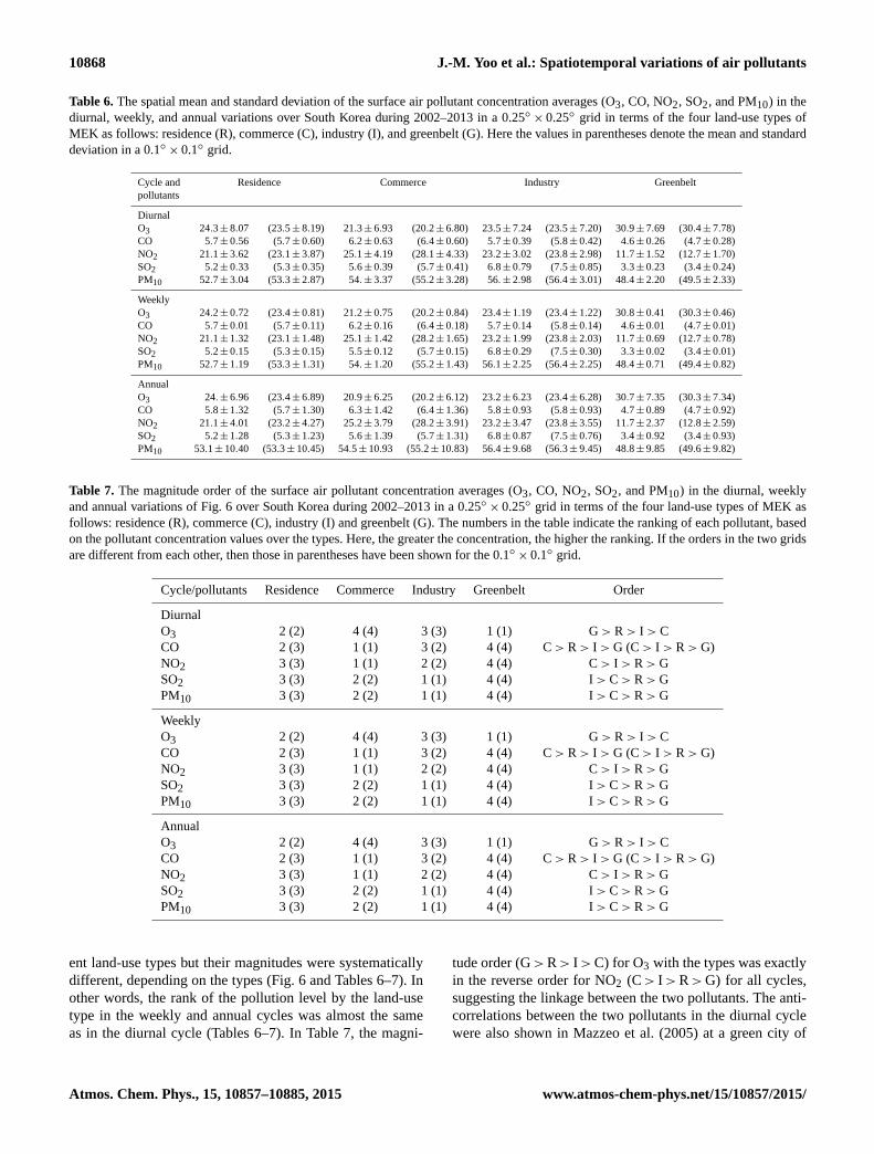
10868 J.-M. Yoo et al.: Spatiotemporal variations of air pollutants
Table 6. The spatial mean and standard deviation of the surface air pollutant concentration averages (O3, CO, NO2, SO2, and PM10) in the
diurnal, weekly, and annual variations over South Korea during 2002–2013 in a 0.25◦× 0.25◦ grid in terms of the four land-use types of
MEK as follows: residence (R), commerce (C), industry (I), and greenbelt (G). Here the values in parentheses denote the mean and standard
deviation in a 0.1◦× 0.1◦ grid.
Cycle and Residence Commerce Industry Greenbelt
pollutants
Diurnal
O3 24.3± 8.07 (23.5± 8.19) 21.3± 6.93 (20.2± 6.80) 23.5± 7.24 (23.5± 7.20) 30.9± 7.69 (30.4± 7.78)
CO 5.7± 0.56 (5.7± 0.60) 6.2± 0.63 (6.4± 0.60) 5.7± 0.39 (5.8± 0.42) 4.6± 0.26 (4.7± 0.28)
NO2 21.1± 3.62 (23.1± 3.87) 25.1± 4.19 (28.1± 4.33) 23.2± 3.02 (23.8± 2.98) 11.7± 1.52 (12.7± 1.70)
SO2 5.2± 0.33 (5.3± 0.35) 5.6± 0.39 (5.7± 0.41) 6.8± 0.79 (7.5± 0.85) 3.3± 0.23 (3.4± 0.24)
PM10 52.7± 3.04 (53.3± 2.87) 54.± 3.37 (55.2± 3.28) 56.± 2.98 (56.4± 3.01) 48.4± 2.20 (49.5± 2.33)
Weekly
O3 24.2± 0.72 (23.4± 0.81) 21.2± 0.75 (20.2± 0.84) 23.4± 1.19 (23.4± 1.22) 30.8± 0.41 (30.3± 0.46)
CO 5.7± 0.01 (5.7± 0.11) 6.2± 0.16 (6.4± 0.18) 5.7± 0.14 (5.8± 0.14) 4.6± 0.01 (4.7± 0.01)
NO2 21.1± 1.32 (23.1± 1.48) 25.1± 1.42 (28.2± 1.65) 23.2± 1.99 (23.8± 2.03) 11.7± 0.69 (12.7± 0.78)
SO2 5.2± 0.15 (5.3± 0.15) 5.5± 0.12 (5.7± 0.15) 6.8± 0.29 (7.5± 0.30) 3.3± 0.02 (3.4± 0.01)
PM10 52.7± 1.19 (53.3± 1.31) 54.± 1.20 (55.2± 1.43) 56.1± 2.25 (56.4± 2.25) 48.4± 0.71 (49.4± 0.82)
Annual
O3 24.± 6.96 (23.4± 6.89) 20.9± 6.25 (20.2± 6.12) 23.2± 6.23 (23.4± 6.28) 30.7± 7.35 (30.3± 7.34)
CO 5.8± 1.32 (5.7± 1.30) 6.3± 1.42 (6.4± 1.36) 5.8± 0.93 (5.8± 0.93) 4.7± 0.89 (4.7± 0.92)
NO2 21.1± 4.01 (23.2± 4.27) 25.2± 3.79 (28.2± 3.91) 23.2± 3.47 (23.8± 3.55) 11.7± 2.37 (12.8± 2.59)
SO2 5.2± 1.28 (5.3± 1.23) 5.6± 1.39 (5.7± 1.31) 6.8± 0.87 (7.5± 0.76) 3.4± 0.92 (3.4± 0.93)
PM10 53.1± 10.40 (53.3± 10.45) 54.5± 10.93 (55.2± 10.83) 56.4± 9.68 (56.3± 9.45) 48.8± 9.85 (49.6± 9.82)
Table 7. The magnitude order of the surface air pollutant concentration averages (O3, CO, NO2, SO2, and PM10) in the diurnal, weekly
and annual variations of Fig. 6 over South Korea during 2002–2013 in a 0.25◦× 0.25◦ grid in terms of the four land-use types of MEK as
follows: residence (R), commerce (C), industry (I) and greenbelt (G). The numbers in the table indicate the ranking of each pollutant, based
on the pollutant concentration values over the types. Here, the greater the concentration, the higher the ranking. If the orders in the two grids
are different from each other, then those in parentheses have been shown for the 0.1◦× 0.1◦ grid.
Cycle/pollutants Residence Commerce Industry Greenbelt Order
Diurnal
O3 2 (2) 4 (4) 3 (3) 1 (1) G> R> I> C
CO 2 (3) 1 (1) 3 (2) 4 (4) C> R> I> G (C> I> R> G)
NO2 3 (3) 1 (1) 2 (2) 4 (4) C> I> R> G
SO2 3 (3) 2 (2) 1 (1) 4 (4) I> C> R> G
PM10 3 (3) 2 (2) 1 (1) 4 (4) I> C> R> G
Weekly
O3 2 (2) 4 (4) 3 (3) 1 (1) G> R> I> C
CO 2 (3) 1 (1) 3 (2) 4 (4) C> R> I> G (C> I> R> G)
NO2 3 (3) 1 (1) 2 (2) 4 (4) C> I> R> G
SO2 3 (3) 2 (2) 1 (1) 4 (4) I> C> R> G
PM10 3 (3) 2 (2) 1 (1) 4 (4) I> C> R> G
Annual
O3 2 (2) 4 (4) 3 (3) 1 (1) G> R> I> C
CO 2 (3) 1 (1) 3 (2) 4 (4) C> R> I> G (C> I> R> G)
NO2 3 (3) 1 (1) 2 (2) 4 (4) C> I> R> G
SO2 3 (3) 2 (2) 1 (1) 4 (4) I> C> R> G
PM10 3 (3) 2 (2) 1 (1) 4 (4) I> C> R> G
ent land-use types but their magnitudes were systematically
different, depending on the types (Fig. 6 and Tables 6–7). In
other words, the rank of the pollution level by the land-use
type in the weekly and annual cycles was almost the same
as in the diurnal cycle (Tables 6–7). In Table 7, the magni-
tude order (G>R> I>C) for O3 with the types was exactly
in the reverse order for NO2 (C> I>R>G) for all cycles,
suggesting the linkage between the two pollutants. The anti-
correlations between the two pollutants in the diurnal cycle
were also shown in Mazzeo et al. (2005) at a green city of
Atmos. Chem. Phys., 15, 10857–10885, 2015 www.atmos-chem-phys.net/15/10857/2015/

J.-M. Yoo et al.: Spatiotemporal variations of air pollutants 10869
Figure 6. The (a) diurnal, (b) weekly, and (c) annual variations in a 0.25◦× 0.25◦ grid of the O3 (ppb), CO (0.1 ppm), NO (ppb), SO2,
(ppb) and PM10 (µg m−3) observations over South Korea during 2002–2013 under the MEK four land-use types as follows: residence (black
circle), commerce (blue cross), industry (red square) and greenbelt (green triangle).
Argentina and Han et al. (2011) in Tianjin, China. However,
the reverse order for O3 was different from those for SO2
and PM10 (I>C>R>G). It is because SO2 and PM10 pol-
lutants were not uniquely associated with vehicle emissions
(Flemming et al., 2005; see also Chen et al., 2001). The same
order for the two pollutants with the land-use types suggested
their emission sources from industrial activities rather than
traffic emissions. It was interesting to note that the greenbelt
area was commonly the lowest for the CNSP pollutants.
Since the primary production of O3 was through photo-
chemical reactions, the O3 started to rise in the morning and
showed its peak at 16:00 before it rapidly decreased (Fig. 6a).
The O3 level was the highest in the greenbelt and the low-
est in the commerce areas, while the levels of the O3 for
the residence and industry regimes were close to each other.
The diurnal cycle of the O3 in this study agreed with that
of Flemming et al. (2005). Two peaks were shown in the
diurnal cycle for CO, NO2, and PM10. The first peak was
www.atmos-chem-phys.net/15/10857/2015/ Atmos. Chem. Phys., 15, 10857–10885, 2015
10870 J.-M. Yoo et al.: Spatiotemporal variations of air pollutants
due to the increasing morning traffic and industrial activity
(Kuttler and Strassburger, 1999). The second peak was due
to the afternoon traffic and reduced boundary layer (Lee et
al., 2014) during and after sunset. The daytime minima of
these species were the results of the increased boundary layer
height (Ulke and Mazzo, 1998; Lal et al., 2000; Han et al.,
2011) as well as the oxidation processes for the chemically
and photochemically reactive CO and NO2, of which diurnal
variations were generally out of phase with those of O3 ex-
cept for the midnight period (Kuttler and Strassburger, 1999;
Lal et al., 2000). The diurnal cycle of the SO2 in the com-
merce type also had two peaks similar to the other pollutants
(CO, NO2 and PM10). The daytime minima could be ex-
plained by the high vertical mixing of their emissions (Meng
et al., 2009). According to the diurnal variations of the CO
and SO2 over a suburban site in the USA, the patterns of their
diurnal cycles were changed seasonally (Chen et al., 2001).
The diurnal cycles of the O3 and NO2 without categorizing
the land-use types were shown in Fig. 6a (O3 and NO2), con-
sistent with those of Han et al. (2011) in Tianjin, China.
The commerce type in the daily, weekly, and annual cycles
was ranked first for the CO and NO2, but it was ranked sec-
ond for the SO2 and PM10 (Fig. 6 and Table 6). The industry
type was ranked first for the SO2 and PM10, but it was ranked
second for the NO2. The residence type in a 0.25◦× 0.25◦
grid was ranked second with the industry regime for the CO,
but it was ranked third for the NO2, SO2, and PM10. These
analyses indicated that the contribution of commerce was
more important for the CO and NO2, and that the contri-
bution of the industry was more important for the SO2 and
PM10. Since the commerce and industry types were asso-
ciated with more vehicles and industrial activity, the CNSP
pollutants in the residence type were lower than for these two
types. Sharma et al. (2014) also reported that the PM10 lev-
els in South Korea and abroad depended on different land-use
types (urban, industry, rural/suburban).
The weekly cycles were analyzed for the different land-use
types (Fig. 6b). The weekly cycle of the five pollutants was
more remarkable in the land-use types with industrial and
commercial activities, particularly in the industry type than
in the greenbelt one. The CO weekly cycle was pronounced
in the commerce type as well as in the industry one. This
implies that the MEK land-use types provided a reasonable
discrimination between natural and anthropogenic pollutant
sources. In general, on Sunday the level of the CNSP pollu-
tants decreased, but the O3 values showed a peak. However,
the degree of the Sunday pollutant values compared to those
averaged for the working days from Tuesday to Friday (here-
after the working day average) varied by the pollutant species
and land-use types. These Sunday lows of the CNSP pollu-
tants and the Sunday high of O3 (the so-called O3 weekend
effect; Larsen et al., 2003) were due to the anthropogenic ac-
tivity that characterized the weekly emission pattern of South
Korea.
In Fig. 6b for O3, less O3 reduction near anthropogenic
sources (e.g., the commerce and residence areas) due to
the decreased NO titration could induce an enhancement
of O3, particularly in the weekly cycle (e.g., Gilge et al.,
2010). The NO2 minimum on Sunday also occurred in Ho-
henpeissenberg, Germany, due to less anthropogenic impact
on weekends than on working days (Gilge et al., 2010). In
Fig. 6b, the NO2 minimum on Sunday (24 % reduction com-
pared to the working day average) in the industry agreed with
that of Beirle et al. (2003) over the industrialized regions (the
USA, Europe and Japan) from the vertical column densities
of tropospheric NO2. The CO reduction on Sunday against
the weekday average was the lowest (3–7 %) among the
CNSP due to its longer lifetime (e.g., Gilge et al., 2010). The
PM10 minimum on Sunday also occurred over a neighboring
country, China (Choi et al., 2008). The O3 Sunday maximum
in the industry type was enhanced by ∼ 15 % with respect to
the weekday average. The weekend effect of O3 varied with
the land-use types: I (15 %)>C (10 %)>R (9 %)>G (4 %).
The increasing O3 during the weekend could be associated
with (1) the decreasing NO2 under the VOC-limited regime
or (2) the behavior of the VOCs (e.g., Sakamoto el al., 2005),
particularly the natural (or biogenic) ones in the greenbelt.
Previous studies showed an increase in the O3 and a decrease
in the NO2 during the weekends in the US and Germany
(Flemming et al., 2005; Atkinson-Palombo et al., 2006). Ac-
cording to Gilge et al. (2010), anti-correlation between O3
and NO2 in their weekly cycles was less pronounced in sum-
mer due to photochemical O3 production than in the other
seasons.
The annual cycle of O3 generally showed a spring–early
summer maximum and a wintertime minimum (Fig. 6c). This
result was consistent with that of Pochanart et al. (1999) at
Oki, Japan, and on a regional scale in northeastern Asia. The
O3 annual variation in the greenbelt presented primary and
secondary peaks in May and October, respectively, reflecting
seasonal changes in the photochemical intensity and Asian
monsoon (Meng et al., 2009; Sarangi et al., 2014). The dou-
ble peak patterns occurred at a regional background site in
northern China in June and September, respectively (Meng
et al., 2009), and at a high-altitude site in northern India
in May and November, respectively (Sarangi et al., 2014).
However, the secondary peak was not clear in the other types
(residence, commerce and industry). This suggested that the
O3 production in a monthly timescale was sensitive to the
local pollutant emissions with the land-use types. The NO2
wintertime maxima could be associated with the fossil fuel
consumption and photochemical oxidation of NO to NO2
(Shon and Kim, 2011), the lower planetary boundary layer
(PBL), and the photolysis rate. The enhanced CO and NO2
values in winter agreed with those of Gilge et al. (2010) over
Hohenpeissenberg, Germany. Tropospheric NO2 concentra-
tions over South Korea also occurred in winter (at least 68 %)
mainly due to local emissions (Mijling et al., 2013).
Atmos. Chem. Phys., 15, 10857–10885, 2015 www.atmos-chem-phys.net/15/10857/2015/

J.-M. Yoo et al.: Spatiotemporal variations of air pollutants 10871
The SO2 maximum in January in its annual cycle was gen-
erally similar to that of SO2 emissions from China of Wang et
al. (2013) (Fig. 6c). The values of the CNSP pollutants were
lowest in June–August, mainly due to the washout effect dur-
ing the rainy period (e.g., Flemming et al., 2005; Meng et
al., 2009; Yoo et al., 2014). Despite the low washout effect
of CO, its reaction with HO radicals was likely to be more
important for the CO sink during the warm season (Stock-
well and Calvert, 1983; Novelli et al., 2003; Gilge et al.,
2010). The declining tendency of the SO2 and NO2 emis-
sions in boreal summer also occurred in China because of
the large-scale monsoon system (Wang et al., 2013). In ad-
dition, the lifetimes of SO2 and NO2 in the atmosphere are
substantially shorter in summer, due to dominant gas-phase
chemistry (e.g., faster photochemical reactions) (Levy II et
al., 1999). This implies that the NO2 transport from China to
South Korea could have more impact over the Korean Penin-
sula during the wintertime dry season than during the sum-
mer and fall (Lee et al., 2014). The springtime PM10 maxima
in its annual variations resulted from Asian Dust and meteo-
rological conditions (Sharma et al., 2014).
In the annual average analyses, the urban effects of the grid
difference (i.e., the pollutant value in the 0.1◦× 0.1◦ grid mi-
nus the value in the 0.25◦× 0.25◦ grid) were quantitatively
the greatest in the types of “commerce” for CO (+0.093
0.1 ppm), NO2(+2.969 ppb), PM10 (+0.711 µg m−3), and
O3 (−0.735 ppb); and “industry” for SO2 (+0.687 ppb)
among the four land-use types (Table 8). This result could
be explained by the emissions of vehicles in the commerce
type and the emissions of factories in the industry type.
6 Pollutant trends of O3, NO2, SO2, CO, PM10, and
OX with respect to land-use types
Figure 7 shows the time series of the spatial averages of
the monthly surface air pollutant anomalies for the five pol-
lutant and OX concentrations in a 0.25◦× 0.25◦ grid over
South Korea during the period from January 2002 to De-
cember 2013 under the following MEK land-use types: res-
idence (black solid), commerce (blue dashed), industry (red
dotted), and greenbelt (green dashed). We calculated linear
trends of the pollutant anomalies with respect to each of the
land-use types. The ± trend values define the 95 % confi-
dence intervals. Trend values of the pollutants are also sum-
marized in Table 9, based on two types of analyses (the
0.1◦× 0.1◦ and 0.25◦× 0.25◦ grids) over the four land-use
types of MEK of residence (R), commerce (C), industry (I),
and greenbelt (G). The magnitude order for the trends of
each of the pollutants over the types has been shown. It
should be noted that the trend values were statistically sig-
nificant except for a few of the NO2 and SO2 cases marked
by an asterisk (∗). Given the different spatiotemporal scales
of the variability for the five pollutants (their scale order:
CO>PM10>O3>SO2>NOx ; Seinfeld and Pandis, 2006),
the behavior of CO was likely to be related to the local, re-
gional, and global effects, but that of NO2 to the local and
regional ones (Gilge et al., 2010).
The CNSP pollutants in South Korea tended to decrease
regardless of the land-use types but, interestingly, the O3 had
an increasing tendency (Fig. 7 and Table 9). Since the five
pollutants showed the same trends (either positive or nega-
tive) over all of the four types, the overall trends could reflect
more the effects of regional emissions than local emissions.
In the O3 formation, for instance, the local contribution re-
lated to the level of primary pollutants (e.g., titration), while
the regional contribution corresponded to the background O3
concentration (Clapp and Jenkin, 2001). The regional back-
ground was likely to be large in the greenbelt area compared
to the other land-use types in view of the reduced weekly cy-
cle in the greenbelt (see also Fig. 6b). The declining trends
of CNSP in a 0.25◦× 0.25◦ grid by the land-use type var-
ied with the values of −0.135∼−0.247 (0.1 ppm yr−1) for
CO,−0.042∼−0.295 (ppb yr−1) for NO2,−0.036∼−0.140
(ppb yr−1) for SO2, and −1.003∼−1.098 (µgm−3 yr−1) for
PM10.
The downward trend of PM10 (∼ 2 %yr−1) in this
study agreed with the result (0.4–2.7 %yr−1) in Sharma et
al. (2014) over major cities in the country during 1996–2010
(Fig. 7f and Table 9). The largest decrease for CO and SO2 in
the industry type was due to the reduced emissions from fac-
tories and power plants (Fig. 7d and e); the largest decrease
for NO2 in the residence type was associated with the re-
duced emission from vehicles (Fig. 7b); the commerce type
was second (CO and SO2) and third (PM10); and the CNSP
trends in the greenbelt type were low (third or fourth) ex-
cept for PM10. However, there was almost no difference in
the PM10 declining trend between the land-use types. Kim
and Shon (2011) reported that the sudden increase in PM10
in spring 2002 occurred due to the enhanced Asian Dust ef-
fect. The systematic decreasing trend of the CNSP pollutants
suggested that the policy for air quality regulation worked
successfully (Sharma et al., 2014).
In contrast to the CNSP case, it was interesting that the
O3 value in a 0.25◦× 0.25◦ grid increased with the rate of
0.352–0.501 (ppb yr−1; ∼ 1.6 %) over the last 12 years, al-
though the CNSP pollutants were reduced (Fig. 7 and Ta-
ble 9). This phenomenon was consistent with Mayer (1999),
who reported that long-term trends of major air pollutants
except for O3 were decreasing, particularly in industrialized
countries, but global O3 levels were increasing during the
early period of the twenty-first century (Cooper et al., 2010).
On the other hand, the standards of the surface O3 concen-
tration for its government control in South Korea are less
than 0.1 ppm for the O3 average during 1 h, and less than
0.06 ppm for the O3 average during 8 h (NIER, 2010). Fur-
thermore, one of three stages of ozone warning in the region
is issued, based on the surface O3 concentration: ozone alert
for 0.12 ppm h−1 or higher, ozone warning for 0.3 ppm h−1
or higher, and ozone grave warning for 0.5 ppm h−1 or higher
www.atmos-chem-phys.net/15/10857/2015/ Atmos. Chem. Phys., 15, 10857–10885, 2015

10872 J.-M. Yoo et al.: Spatiotemporal variations of air pollutants
Figure 7. Time series of the monthly surface air pollutant anomalies in a 0.25◦× 0.25◦ grid of the (a) O3 (ppb), (b) NO2 (ppb), (c)
OX (ppb), (d) CO (0.1ppm), (e) SO2 (ppb), and (f) PM10 (µg m−3) observations over South Korea during the period from January 2002
to December 2013 under the following MEK land-use types: residence (black solid), commerce (blue dashed), industry (red dotted) and
greenbelt (green dashed). The ± trend values define the 95 % confidence intervals.
Atmos. Chem. Phys., 15, 10857–10885, 2015 www.atmos-chem-phys.net/15/10857/2015/

J.-M. Yoo et al.: Spatiotemporal variations of air pollutants 10873
Table 8. Comparisons of the climatological annual averages over South Korea during 2002–2013, based on the two types of spatial-scale
analyses of the 0.1◦× 0.1◦ and 0.25◦× 0.25◦ grids. The 0.1◦× 0.1◦ grid averages (compared to those of 0.25◦× 0.25◦) generally tend to
show the characteristics in big urban cities rather than in small suburban cities, because the air pollution monitoring stations are more densely
located in the former areas.
Air pollutant Average (0.1◦× 0.1◦) minus average (0.25◦× 0.25◦)
Residence Commerce Industry Greenbelt
O3 (ppb) −0.513 −0.735 0.181 −0.342
CO (0.1 ppm) −0.067 0.093 0.052 0.009
NO2 (ppb) 2.020 2.969 0.573 0.767
SO2 (ppb) 0.036 0.123 0.687 0.033
PM10 (µgm−3) 0.270 0.711 −0.012 0.409
Table 9. Trends of surface air pollutants (O3, NO2, OX, CO, SO2 and PM10) over South Korea during 2002–2013, based on the three types
of analyses (0.1◦× 0.1◦ grid and 0.25◦× 0.25◦ grid) over the four land-use types of the MEK of residence (R), commerce (C), industry (I),
and greenbelt (G). The magnitude order for the trends of each of the pollutants over the types has been shown in the figures. The ± trend
values indicate the 95 % confidence intervals. It should be noted that the trend values are statistically significant except for some of the NO2
and SO2 cases, marked by an asterisk (∗).
Residence Commerce Industry Greenbelt Trend Order
0.25◦× 0.25◦
O3 (ppbyr−1) 0.501± 0.098 0.407± 0.095 0.352± 0.093 0.369± 0.094 Increase R> C> G> I
NO2 (ppbyr−1) −0.295± 0.081 −0.042± 0.088∗ −0.135± 0.084 −0.100± 0.053 Decrease R> I> G> C∗
OX (ppbyr−1) 0.205± 0.107 0.365± 0.103 0.231± 0.113 0.260± 0.103 Increase C> G> I> R
CO (0.1 ppmyr−1) −0.202± 0.021 −0.210± 0.021 −0.247± 0.025 −0.135± 0.022 Decrease I> C> R> G
SO2 (ppbyr−1) −0.036± 0.024 −0.114± 0.028 −0.140± 0.029 −0.060± 0.016 Decrease I> C> G> R
PM10 (µgm−3 yr−1) −1.038± 0.459 −1.014± 0.456 −1.003± 0.480 −1.098± 0.485 Decrease G> R> C> I
0.1◦× 0.1◦
O3 (ppbyr−1) 0.545± 0.096 0.462± 0.092 0.340± 0.094 0.326± 0.095 Increase R> C> I> G
NO2 (ppbyr−1) −0.240± 0.083 −0.078± 0.092∗ −0.054± 0.084∗ −0.023± 0.054∗ Decrease R> C∗ > I∗ > G∗
OX (ppbyr−1) 0.304± 0.108 0.396± 0.106 0.299± 0.110 0.300± 0.102 Increase C> R> G> I
CO (0.1 ppmyr−1) −0.175± 0.021 −0.204± 0.020 −0.246± 0.025 −0.124± 0.022 Decrease I> C> R> G
SO2 (ppbyr−1) −0.019± 0.023∗ −0.104± 0.027 −0.177± 0.030 −0.050± 0.015 Decrease I> C> G> R
PM10 (µgm−3 yr−1) −1.374± 0.535 −1.290± 0.474 −0.926± 0.492 −1.049± 0.485 Decrease R> C> G> I
concentration. While the surface O3 level varies seasonally
from 0.018 ppm in winter to 0.035 ppm in spring in South
Korea (Table 5), there have been 84 times for 28 areas of the
ozone alert, and 83 times for 27 areas of the ozone warn-
ing on an annual basis during the 12-year period of this
study (https://seoulsolution.kr/content/). Given the increas-
ing trends of O3 found in this study (Fig. 7a), it will be impor-
tant to understand possible factors causing such trends. Seo et
al. (2014) reported an increase in the O3 (+0.26 ppb yr−1) in
46 cities in South Korea from 1999 to 2010. Also, the O3 in-
crease (+0.48 ppb yr−1) from 1990 to 2010, which was more
consistent with our results, generally occurred for all of the
seasons and day/night at most of the surface monitoring sites
(Lee et al., 2014). This tendency was commonly shown in
the two types of spatial grid analyses, possibly due to grow-
ing background O3 (Table 9).
The possibility of enhanced regional (background) O3 as
well as the local effect of the O3 titration could be supported
by the significant upward trends (0.205–0.396 ppb yr−1; Ta-
ble 9 and Fig. 7c) of the total oxidant (OX) despite the down-
ward trends of the O3 precursors (e.g., NO2, CO, and PM10).
Specifically, the significant positive trends of the OX values
(0.260–0.300 ppb yr−1) in the greenbelt type in the two kinds
of spatial grids suggested the increase in background O3 in-
duced by its inflow from the regional scale, rather than the lo-
cal scale. The upward trends of the OX in both the grids were
commonly more pronounced in the commerce type than the
other types, but the cause was unknown.
A positive trend of tropospheric ozone (3.1 % yr−1) was
clearly seen over Beijing from 2002 to 2010 in Wang et
al. (2012), who emphasized a contribution in the downward
O3 flux from the stratosphere for the period. In spite of the
CNSP decreasing trends in a 0.25◦× 0.25◦ grid (i.e., less ur-
ban features), the NO2 tendency in a 0.1◦× 0.1◦ grid (i.e.,
more urban features) was not evident except for the resi-
dence (Table 9). Thus, the government regulation for NO2
www.atmos-chem-phys.net/15/10857/2015/ Atmos. Chem. Phys., 15, 10857–10885, 2015

10874 J.-M. Yoo et al.: Spatiotemporal variations of air pollutants
might not be very successful in large cities due to its diverse
sources. Xu et al. (2008) suggested that the increased vari-
ability of the surface O3 at a station in eastern China was
mainly associated with the enhanced NOx emission near the
station.
The O3 levels, which were related to the spatial variability
in the local precursor emissions, were expected to vary with
the land-use types. Seo et al. (2014) revealed that the long-
term trends of the local precursor emissions in O3 in South
Korea could affect the O3 trends locally, and in the country,
significant enhancement of the background O3 negatively af-
fected the air quality. In order to understand the negative re-
lationship in trend between O3 and CNSP pollutants, partic-
ularly NO2, we have investigated the relationship (i.e., cor-
relation and weekly cycle) among O3, NO2 and VOCs with
the land-use types further in Sects. 6 and 7. In this study,
we focused on two issues: (1) which condition in view of
the O3 control in South Korea was more dominant, the VOC
sensitivity or the NO2 sensitivity? (2) Did this condition sig-
nificantly depend on the land-use types and the weekly cy-
cles of the pollutants? The negative relationship between O3
and NO2 is expected in the VOC-limited condition. The local
effect of the pollutants compared to the regional (i.e., back-
ground) effect can be shown, based on their weekly varia-
tions at each station of the four land-use types.
7 Correlation between O3 and NO2 with land-use types
As shown in Fig. 7, the increasing O3 trend was the oppo-
site of the decreasing CNSP trends. The O3 trends could be
affected by interannual variations of the pollutant emissions
(e.g., NOx and VOCs) from their various sources and of the
meteorological conditions (Kim et al., 2006). In view of the
“O3 control” strategy, the relationship between O3 and NOx(and the VOCs) was examined in many previous studies (e.g.,
Mazzeo et al., 2005; Han et al., 2011). There were various
factors affecting the O3: (1) local precursor emissions (e.g.,
NO2, VOCs, and CO); (2) O3 transport and its precursors
from the local and remote sources; and (3) meteorological
conditions (Seo et al., 2014). In this study we focused on
the relationships on the local (grid) and regional (nationwide)
scales in South Korea.
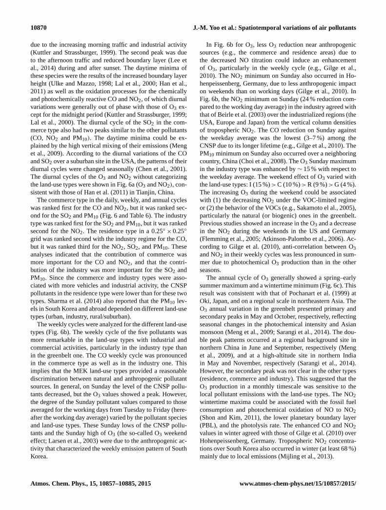
Figure 8 shows scatter diagrams of the O3 versus NO2
from the monthly anomalies of Fig. 7 in South Korea under
the four land-use types: (a) residence (black circle), (b) com-
merce (blue cross), (c) industry (red square) and (d) green-
belt (green triangle). The sample number in the monthly
anomaly time series of each pollutant was 144 during 2002–
2013. The temporal correlation coefficient (r) between the
anomalies of the two pollutants was given together with the
regression dotted line. The correlations between the anoma-
lies in the residence and commerce types were statistically
significant at a significance level of p < 0.01 (i.e., either
r > 0.194 or r <−0.194). The correlation was also signifi-
cant at p < 0.05 (i.e., either r > 0.137 or r <−0.137) in the
industry type, but not significant in the greenbelt type due to
the least NO2 emissions. Therefore, these results indicated
that the NO2 emissions from vehicles in the residence and
commerce areas were highly related to the O3 change on the
long-term timescale (Fig. 8a–b). Also, the NO2 probably af-
fected the O3 in the industry type. The above results agreed
with those of Seo et al. (2014), who reported that the long-
term O3 variation over South Korea was similar to that of
NO2, but their trends were spatially different.
Figure 9 presents the relationship between O3 and NO2 in
terms of the climatological annual averages over South Ko-
rea during 2002–2013 under the MEK four land-use types
of residence (R), commerce (C), industry (I), and greenbelt
(G). The relationship was derived from the data of all of the
283 stations, which were individually specified by one land-
use type among the four types (Fig. 9a). Since the stations
of residence were located nationwide (i.e., more than half of
all the stations), the relationship could be spatially different
due to the population-related traffic emissions. Furthermore,
the NO2 decreasing trends in a 0.1◦× 0.1◦ grid (Table 9)
were found to be significant only in the residence area, but
not in the other types, despite the government control efforts
(e.g., Shon and Kim, 2011). Note that the pollutant trends
in a 0.25◦× 0.25◦ grid were given in Fig. 7, where the NO2
trends were significant except for commerce among the four
land-use types. In order to further investigate the relationship
within the residence areas based on the population size, we
subdivided the locations of the 154 residence-type stations
of Fig. 1a by the three regions (Fig. 9b) as follows: (i) the
capital city of the country, Seoul (red circle), (ii) the SMA
(green circle) except for Seoul, and (iii) outside of the SMA
(blue circle). Therefore, the SMA is composed of (i) Seoul
and (ii) the SMA except for Seoul. The 20 and 50 % portions
of the entire population in South Korea (∼ 50.5 million in
2014) lived in Seoul and the SMA, respectively. There were
more traffic emissions in the SMA than outside of the SMA,
particularly in the residence types.
A very strong correlation (p < 0.01) of PM10 with the CO
and NO2 in their monthly data set time series (Fig. 7) was
likely to be associated with the traffic emission sources (see
also Shon and Kim, 2011, and Sharma et al., 2014). The cor-
relations (0.42–0.56) in the residence and commerce were
greater than those (0.32–0.47) in the greenbelt and indus-
try, which was probably due to the vehicle emissions. In
other words, more traffic emissions, which were related to
the population density, were expected in Seoul than in the
SMA excluding the capital city. The residence and commerce
types were dominant in Seoul (Fig. 1a and b), while the resi-
dence and industry types predominantly existed in the SMA
(Fig. 1b and d). Figure 9c is the same as Fig. 9a except for
excluding the data in the SMA residence areas. Figure 9d is
the same as Fig. 9a except for the O3 and NO2 relationships
in the residence only over the three different regions shown
Atmos. Chem. Phys., 15, 10857–10885, 2015 www.atmos-chem-phys.net/15/10857/2015/
J.-M. Yoo et al.: Spatiotemporal variations of air pollutants 10875
Figure 8. Scatter diagrams of the monthly anomalies of O3 (ppb) versus NO2 (ppb) in South Korea during the period from January 2002
to December 2013 under the four land-use types; (a) residence (black circle), (b) commerce (blue cross), (c) industry (red square), and (d)
greenbelt (green triangle). The correlation coefficient (r) and the regression dotted line are also given.
in Fig. 9b. In Fig. 9d, the relationships over the three regions
are shown in three colors, respectively.
The NO2 value was the highest in the commerce areas over
South Korea (Fig. 9a and c; Table 10). The NO2 concen-
tration was estimated in the following order: commerce (C:
31.3)> residence (R: 25.9)> industry (I: 24.3)> greenbelt
(G: 13.3) (Fig. 9a). However, when the NO2 (ppb) values in
the region excluding the 74 SMA residence stations were ex-
amined, the order of the residence and industry areas was dif-
ferent from the previous case as follows: I (24.3)>R (20.3)
(Fig. 9c). This result suggested that there were more NO2-
related traffic emissions (5.6 ppb) in the SMA residence ar-
eas than in the nationwide residence areas (Fig. 9a and c).
The maxima (30.2 ppb) of the O3 concentrations occurred in
the greenbelt areas, while their minima were shown in the
commerce areas (Fig. 9a and c). The order of magnitude of
the O3 was the opposite of that of the NO2, showing an in-
verse relationship between the two pollutants (see also Han
et al., 2011).
The traffic-induced pollutants were mainly NO, CO and
PM10, as well as VOCs, and the secondary trace gases of
O3 and NO2 could be formed from these precursor sub-
stances during the photochemical reactions (Kuttler and
Strassburger, 1999). They reported the inverse relationship
of the O3 versus NO2 within the urban areas (Essen, Ger-
many) with the following five land-use types: motorway, the
main and secondary roads, residence and greenbelt. The three
types of the roads and motorway could correspond to the
commerce areas in our study, particularly in the urban area
(e.g., the SMA). Overall, our results were consistent with
those of Kuttler and Strassburger (1999), who showed that
the higher O3 concentration was formed in urban green areas
in the summer during intensive solar radiation, due to the rel-
atively low share of NO in the total concentrations of NO2 in
the greenbelt areas. However, an inverse relationship has also
been found in winter (Table 10). The consistency in the rela-
tionship of O3 versus NO2 between the two studies supported
the validation of the MEK classification method for the four
www.atmos-chem-phys.net/15/10857/2015/ Atmos. Chem. Phys., 15, 10857–10885, 2015

10876 J.-M. Yoo et al.: Spatiotemporal variations of air pollutants
Figure 9. Climatological annual averages of the O3 (ppb) versus NO2 (ppb) over South Korea during 2002–2013 under the MEK four land-
use types of residence (R), commerce (C), industry (I), and greenbelt (G). (a) O3 versus NO2 at all 283 stations in South Korea. The number
in the upper-right-side panel of the figure indicates the number of stations. (b) Locations of 154 “residence-type” stations subdivided by the
three regions as follows: (i) Seoul (red circle), (ii) the Seoul Metropolitan Area (SMA; green circle) except for Seoul, and (iii) outside of the
SMA (blue circle). The rectangular area in Fig. 9b indicates that the SMA has been enlarged on the right side. (c) Same as Fig. 9a except for
exclusion of the O3 and NO2 observations of the SMA residential region. (d) Same as Fig. 9a except for using the O3 and NO2 only in the
“residence” type under the three different regions of Fig. 9b. The mean values and standard deviations for the annual values of NO2 and O3
in each of the types are indicated in Fig. 9a, b, and d.
land-use types. According to the monthly mean analysis of
Xu et al. (2008) at a background station in eastern China,
the negative correlation between O3 and NOx was found in
the lowest 5 % of ozone in cold seasons than in the high-
est 5 % in warm seasons. Overall, the inverse relationship in
Fig. 9a and c of this study, which systematically showed in
the O3 magnitude order (G>R> I>C; see also Table 6 in
a 0.25◦× 0.25◦ grid) over the stations excluding the SMA
residence areas in a non-grid, agreed well with the previous
studies, suggesting that the four MEK land-use type classifi-
cation was made reasonably.
As shown in Figs. 1a and 9a, the number of nationwide
residence stations was the largest among the four land-use
types. The spatial dependence of the O3 versus NO2 rela-
tionship over the three different residence types (Fig. 9b;
Seoul, the SMA except for Seoul, and outside of the SMA)
where the amounts of traffic emissions were expected to be
different due to the number density of automobiles per unit
area (as shown in Fig. 1d) was interesting to note. Further-
more, relatively short-lived NO2 compared to the other pol-
lutants (CO, PM10, O3, and SO2) in this study was used as a
good indicator to reflect local and regional anthropogenic ef-
fects (Gilge et al., 2010). Although the SMA included Seoul,
the residence region was separated into two sub-regions in
this study in order to analyze the difference in the pollu-
tants between them (Fig. 9d and Table 10). Heavier traf-
fic generally occurred in Seoul than in the rest of the ar-
eas in the SMA. The NO2 (ppb) concentrations in the res-
Atmos. Chem. Phys., 15, 10857–10885, 2015 www.atmos-chem-phys.net/15/10857/2015/

J.-M. Yoo et al.: Spatiotemporal variations of air pollutants 10877
Table 10. Climatological average value of O3 (ppb) and NO2 (ppb) over South Korea during 2002–2013 in terms of the MEK four land-use
types (residence, commerce, industry and greenbelt) over the 283 total stations and the 209 stations excluding the 74 SMA residence areas,
respectively. The spatial variation in the pollutant concentrations for the individual type is presented with the standard deviation of ± values.
The number in the parentheses indicates the ranking of each pollutant, based on concentration value over the type.
All stations Stations excluding the SMA residence areas
Air pollutant O3 NO2 O3 NO2
Land-use type
〈Annual 〉
Residence 22.4± 4.32 (3) 25.9± 8.15 (2) 25.0± 4.03 (2) 20.3± 4.94 (3)
Commerce 19.2± 4.85 (4) 31.3± 12.00 (1)
Industry 23.4± 4.32 (2) 24.3± 6.89 (3) 23.4± 4.32 (3) 24.3± 6.89 (2)
Greenbelt 30.2± 7.83 (1) 13.3± 9.63 (4)
〈Winter only 〉
Residence 15.4± 4.91 (3) 30.6± 9.04 (2) 18.3± 4.80 (2) 24.4± 6.0 (3)
Commerce 13.2± 4.28 (4) 34.6± 11.29 (1)
Industry 16.7± 4.43 (2) 27.8± 7.52 (3) 16.7± 4.43 (3) 27.8± 7.52 (2)
Greenbelt 24.4± 8.72 (1) 16.3± 11.27 (4)
idence areas over South Korea were estimated in the fol-
lowing order: Seoul (35.5± 2.53) > SMA except for Seoul
(31.7± 4.03)> outside of the SMA (20.3± 4.94) (Fig. 9d).
In the residence, there were pronounced reductions in the
mean and standard deviation values of NO2 due to the greater
distance from the main traffic-induced pollution sources in
the SMA including Seoul. The order of the O3 (ppb) con-
centrations was the opposite of that for the NO2 as follows:
outside of the SMA (25.0± 4.03)>SMA except for Seoul
(19.8± 1.74)>Seoul (18.6± 1.30). As a result, the MEK
residence type, which had large variations in the two pollu-
tant concentrations, could be required to be subdivided in the
future in view of the O3 versus NO2 relationship. However,
the difference in the concentrations between the two regions
within the SMA (i.e., Seoul and the SMA except for Seoul)
was relatively small compared to that between the SMA and
outside of the SMA, due to their transport over the geograph-
ically neighboring locations.
8 Weekend effect of the O3, NO2, VOCs, OX, and
VOC / NO2 with land-use types
Since the O3 formation at the surface can depend on two ma-
jor precursors (i.e., NOx and VOCs; Larsen et al., 2003) and
the ratio of the NOx and VOCs (e.g., Pudasainee et al., 2006),
the relationship among these three pollutants (O3, NO2 and
VOCs) was examined in the weekly cycles of many previ-
ous studies (e.g., Gilge et al., 2010). The impact of the VOC
emission controls on the O3 trend in northwestern Europe
was discussed in Derwent et al. (2003). Both the VOC emis-
sion data and the observations of atmospheric concentrations
of VOCs in South Korea were lacking compared to those
of the O3 and NO2, and thus the VOC observational sites
and records were sparse (as shown in Fig. 1e and Table 2).
Figure 10 shows the weekly variations in the VOCs (green
triangle), O3 (red square) and NO2 (blue rectangle) concen-
trations at nine photochemical air pollution monitoring sta-
tions in South Korea from 2007 under the MEK four land-use
types. The land-use types at the stations available for simul-
taneous observations (O3, NO2, and VOCs) were four res-
idences (the sites of Bulgwang, Daemyoung, Gocheon and
Goowol), three greenbelts (Seokmo, Taejong and Gwanin), a
commerce area (Simgok) and an industry area (Joongheung).
The weekly cycle of the three pollutants was conspicuous
in the residence and commerce areas (Fig. 10a–e). In the ar-
eas, the NO2 and VOC values were higher by 20–33 % on
the weekdays than on the weekends due to variations in an-
thropogenic activity, while the O3 value was higher by 17–
21 % on the weekends. The VOC increase on weekdays in
the residence (Bulgwang) was probably due to vehicle emis-
sions (e.g., Anthwal et al., 2010). The so-called weekend ef-
fect has been reported by Marr and Harley (2002a, b) and
Fujita et al. (2003a, 2003b) over the LA basin, with higher
O3 concentrations on the weekends than on the weekdays.
Marr and Harley (2002b) also found the weekly patterns of
the lower NOx and VOCs during weekends, out of phase
with the higher O3. Qin et al. (2004b) revealed that VOC-
limited conditions for O3 production and the NOx-emission
reduction on weekends could be associated with the week-
end effect of O3 in southern California. In contrast to the res-
idence and commerce areas, however, the weekly cycles of
the three pollutants are not clear in the greenbelts and indus-
try areas (Fig. 10f–i). In view of the negligible weekly cycle
in the industry areas (Fig. 10f), the primary source of the cy-
cle was traffic emission rather than the industrial factory ac-
tivity. Since the industry station at Joongheung was located
near the coast (Fig. 1e; red square), it could also have been in-
fluenced by meteorological factors (e.g., sea breeze). In addi-
tion, more observations for the industry and commerce types
www.atmos-chem-phys.net/15/10857/2015/ Atmos. Chem. Phys., 15, 10857–10885, 2015

10878 J.-M. Yoo et al.: Spatiotemporal variations of air pollutants
were required for detailed analysis, because the photochem-
ical (VOC) data in the two types were only available at a
single station, respectively (Fig. 10e–f). In summary, a more
local effect influenced the three pollutants in the residence
and commerce areas, while a regional (background) effect
dominated in the greenbelt and industry areas.
It is interesting to note that the averages of the three pollu-
tants at Simgok in the commerce type (Fig. 10e) were highly
contrasted with those at Seokmo (Fig. 10g) in the greenbelt
type. In other words, the O3 level among the nine stations
(Fig. 10) was the highest at Seokmo but relatively low at Sim-
gok. However, the NO2 and VOC values had an opposite ten-
dency with the O3 case, showing their high values at the for-
mer (commerce) site and their low values at the latter (green-
belt) site. According to the study of Seo et al. (2014), larger
NOx emissions over the metropolitan cities in the short term
and seasonality showed lower O3 minima because of NOxtitration and a nocturnal NOy chemical process. They also
reported that the higher O3 level near the Seokmo greenbelt
(i.e., Ganghwa) were induced due to lower NOx emissions
and the regional O3 influxes from both the Yellow Sea (and
China) and the SMA.
The decrease in local VOCs reduced O3 with a reason-
able amount of NO2, and the ratio of VOCs to NOx (i.e.,
VOC /NOx) was an important factor for the O3 control strat-
egy (Marr and Harley, 2002a, b; Fujita et al., 2003a, b).
Decreasing NOx tended to increase O3 formation when the
VOC /NOx ratio was less than the threshold values of 8–
10 (Larsen et al., 2003). In addition, decreasing NOx tended
to decrease O3 formation when the ratio was greater than
the threshold values. In this study, the NO2 value instead of
NOx was introduced for an approximate calculation of the
ratio. The amounts of NO2 approximately corresponded to
77–95 % of the amount of NOx over a background station in
northern China (Meng et al., 2009). Therefore, the ratios used
in this study (i.e., VOC /NO2) may be overestimated com-
pared to those of VOC /NOx . The inter-relationship among
the three pollutants was statistically examined in view of the
individual role of NO2 and VOCs for the O3 control in this
study.
Figure 11 shows the scatter diagrams of the long-term av-
erages of the (a) VOCs vs. NO2, (b) O3 vs. VOCs, (c) O3
vs. NO2, and (d) O3 vs. VOC /NO2 at the photochemical
stations under the following four land-use types: residence
(black circle), commerce (blue cross), industry (red square),
and greenbelt (green triangle). The correlation coefficient
and the dotted regression line were also given. The spatial co-
efficients were statistically significant for the cases of O3 vs.
NO2 at p < 0.01 (i.e., r <−0.750; Fig. 11c) and for VOCs
vs. NO2 at p < 0.05 (i.e., r > 0.583; Fig. 11a). Meanwhile,
the correlations were not significant for the other two cases
(O3 vs. VOCs and O3 vs. VOC /NO2) (Fig. 11b and d).
The significant positive correlation between the VOCs and
NO2 might have been due to their common anthropogenic
sources (e.g., transportation and industrial activities). Nine
VOC values in Fig. 11a–b were systematically separated by
their types in view of magnitude. However, the residence val-
ues for the NO2 and O3 cases were not distinct from the in-
dustry case, due to their broad-range values in the residence
areas (Fig. 11c). Overall, the pollutant values at the four res-
idences and three greenbelts are systematically clustered in
the two-dimensional domains of Fig. 11, supporting the idea
that the MEK land-use types are reasonable.
Figure 12 presents weekly variations of the OX and
VOC /NO2 values at each of the nine photochemical sta-
tions of Fig. 10. The equally weighted averages with respect
to the four land-use types were also given for the OX and
VOC /NO2 in Fig. 12a–b (the grey cross dashed line), re-
spectively. The weekend effect of OX in the residence and
commerce was evident, while it was negligible in the green-
belt area (Fig. 12a). This contrast suggested the reduction
of order of OX (ppb) is C (57.4)>R (53.6)> I (50.7)>G
(45.4) (Table 11). The weak weekly cycle of OX in the green-
belt may be associated with the OX background level, al-
though there was about a 9 ppb difference in OX between the
greenbelt stations.
The average of VOC /NO2 (the grey cross dashed line) did
not show a clear weekly cycle (Fig. 12b). The weekly cycles
of the ratio were almost negligible except for some stations.
The industry type at Joongheung had a minimum on Tues-
day in the weekly cycle, and its cause was unknown. Some
weekend effects of the reduced ratio (i.e., the decrease on
Saturday–Monday) at Daemyoung and Gocheon in the resi-
dence area occurred possibly due to the NO2 reduction from
less anthropogenic traffic emission. The ratio values tend to
be relatively low in the greenbelt (2.0–5.3) and residence
(2.6–3.5) areas. The four-type average was 6.6 (Table 11).
Based on the average result at the photochemical stations, the
VOC-limited chemistry over South Korea was more common
than the NOx-limited one in the industry (Joongheung). As a
result, except for the Joongheung station, the NO2 decrease
on weekends could result in the enhanced O3 production at
the other eight stations in South Korea. This phenomenon
was more conspicuous in the residence and commerce areas
(five stations) due to the weekly cycle of anthropogenic vehi-
cle emission than in the greenbelt areas (three stations). The
ratio result in this study over the SMA was consistent with
that of Jin et al. (2012), who reported that the areas of the
Seoul and Incheon were VOC-limited using the Ozone Iso-
pleth Plotting Package for Research (OZIPR) model. Also
in the model study, 24 areas in Gyeonggi-do that approxi-
mately included the SMA except the two cities were equally
either VOC-limited or neutral. However, the modeling had
some limitations due to inaccuracy in emission inventories
and transport.
Figure 13 and Table 11 summarized the long-term sur-
face air pollutant averages (O3, NO2, OX, VOCs, and
VOC /NO2) at the nine photochemical stations over South
Korea since 2007 in terms of the four MEK land-use types.
The values (O3, NO2, VOCs, and VOC /NO2) in the bar
Atmos. Chem. Phys., 15, 10857–10885, 2015 www.atmos-chem-phys.net/15/10857/2015/

J.-M. Yoo et al.: Spatiotemporal variations of air pollutants 10879
Figure 10. The weekly variations in the VOCs (green triangle), O3 (red circle), and NO2 (blue rectangle) concentrations at the nine pho-
tochemical air pollution monitoring stations in South Korea since 2007 under the MEK four land-use types as follows: residence (R),
commerce (C), industry (I), and greenbelt (G). Please see Table 2 for the observational period at each of the VOC stations. For convenience,
the terminology of “VOC” in the figures means “VOCs” in the text.
Table 11. The spatial mean values of the long-term surface air pollutant concentration averages (O3, NO2, OX, VOC, and VOC/NO2) at
nine of the photochemical air pollution monitoring stations of the MEK over South Korea since 2007 in terms of the four MEK land-use
categories as follows: residence (R), commerce (C), industry (I), and greenbelt (G).
Air pollutant Residence Commerce Industry Greenbelt Average
O3 (ppb) 21.8± 1.24 22.0 31.0 35.5± 0.43 27.6
NO2 (ppb) 31.8± 2.18 35.5 19.7 9.9± 0.39 24.2
OX=O3+NO2 (ppb) 53.6± 1.00 57.4 50.7 45.4± 0.29 51.8
VOC (ppbC) 112.2± 14.84 308.3 199.6 31.2± 2.14 162.8
VOC/NO2 3.6± 0.27 8.7 10.2 3.9± 0.13 6.6
graph in the figure were shown in the colors of orange,
blue, grey and red, respectively. The OX values were given
with the diamond symbol in green. The OX value, com-
posed of NO2-independent and NO2-dependent parts, was
utilized in order to understand the regional background O3
concentration (i.e., the NO2-independent one) (Mazzeo et
al., 2005; Han et al., 2011). According to their studies, the
OX values did not necessarily correlate with the levels of lo-
cal primary pollution (i.e., NOx-dependent). The residence
values of the NO2 and VOCs were 3–4 times greater than
the greenbelt values. The NO2 (ppb) concentrations in the
four land-use types were estimated to be in the following
order: commerce (C; 35.5)> residence (R; 31.8)> industry
(I; 19.7)> greenbelt (G; 9.9). The VOCs (ppbC) order was
C (308.3)> I (199.6)>R (112.2)>G (31.2). Therefore, the
anthropogenic sources of the VOC pollutants in the com-
merce and industry areas were likely to be more dominant
than the natural ones. Nguyen et al. (2009) also reported the
www.atmos-chem-phys.net/15/10857/2015/ Atmos. Chem. Phys., 15, 10857–10885, 2015

10880 J.-M. Yoo et al.: Spatiotemporal variations of air pollutants
Figure 11. Scatter diagrams of the long-term averages of (a) VOCs versus NO2, (b) O3 versus VOCs, (c) O3 versus NO2, and (d) O3 versus
the ratio of VOCs /NO2 at nine of the photochemical air pollution monitoring stations over South Korea since 2007 under the following
four land-use types: residence (black circle), commerce (blue cross), industry (red square), and greenbelt (green triangle). The correlation
coefficient (r) and the regression dotted line were also given.
relative abundance of anthropogenic VOCs emissions com-
pared to natural ones at a site in Seoul in 2004. The VOC or-
der in the residence and commerce areas was different from
the NO2 order, probably due to the different anthropogenic
sources of the two different pollutants. On the other hand,
the greenbelt and industry O3 averages were greater than the
residence and commerce ones by approximately 50 %. The
order for O3 (ppb) was G (35.3)> I (31.0)>C≈R (21.8–
22.0), which was almost opposite to the NO2 case.
The ratio values of the VOC /NO2 (3.6–8.7) in the resi-
dence, greenbelt, and commerce areas were generally smaller
than the threshold values, while the ratio in the industry was
the largest (10.2) of the four types (Table 11 and Fig. 13).
The order for the ratio was I (10.2)>C (8.7)>G (3.9)>R
(3.6). Therefore, the eight stations except for the industry
area among the nine photochemical stations belonged to the
VOC-limited range that was defined as having the ratio value
of less than 8–10 (see also Larsen et al., 2003). The industry
station corresponded to the NOx-limited chemistry. Higher
O3 levels on weekends (except in industry) could be associ-
ated with lower NO2 values on weekends under the VOC-
limited O3 formation regime. This tendency was also shown
in the greenbelt as well as in the residence and commerce
areas, although it was not as evident in the residence and
commerce areas. This result was similar to the analysis of
Marr and Harley (2002b) in California. They found that a
shift in O3 formation from NOx-limited to VOC-limited con-
ditions in the region could result from the reduction of VOCs
more than that of NOx . Based on the number of individual
land-use-type stations and their distribution over South Ko-
rea (Fig. 1), the VOC control strategy for the O3 reduction
in this country was overall more effective than the NOx con-
trol strategy. However, since the sample number of the photo-
chemical stations in this study was limited particularly in the
commerce and industry areas, the strategy could be shifted
with the land-use types and more photochemical station data
were needed for a more rigorous result. On the one hand, the
VOC-limited condition was also shown in Shanghai, China
Atmos. Chem. Phys., 15, 10857–10885, 2015 www.atmos-chem-phys.net/15/10857/2015/

J.-M. Yoo et al.: Spatiotemporal variations of air pollutants 10881
Figure 12. Weekly variations in the (a) OX and (b) VOCs /NO2 values 2007 at nine of the photochemical air pollution monitoring stations
of the MEK in South Korea. Please see Table 2 for the observational period at each of the VOC stations.
(Tie et al., 2013). On the other hand, according to the one-
dimensional photochemical study of Liu et al. (2012) in Bei-
jing, China, the reduction of either NO2 or VOCs could in-
duce the decrease in O3 production in the transition regime
from VOC-limited to NOx-limited, which was more pro-
nounced in the PBL. Lower VOCs in greenbelt areas than
other land-use types in Fig. 10 indicate a weak contribution
of the anthropogenic VOCs in greenbelt areas. Therefore, the
competing role between biogenic and anthropogenic sources
highly depends on the location and conditions.
The OX values ranged from a minimum (45.4 ppb) in the
greenbelt areas to a maximum (57.4 ppb) in the commerce
area, indicating less variability than the other pollutant val-
ues (O3, NO2, and VOCs) (Fig. 13 and Table 11). This re-
sult agreed with the analysis of Mazzeo et al. (2005) in a
green area of Argentina. The OX values in some areas in
Taiwan were almost constant in previous studies (Chen et
al., 2002; Chou et al., 2006). This result suggested that the
“NOx-titration” effect (e.g., Chou et al., 2006) was an im-
portant mechanism for the O3 change. The temporal O3 lev-
els in the SMA and some inland areas were lower than those
in the greenbelt and coastal areas due to the NOx-titration ef-
fect (Kuttler and Strassburger, 1999; Ghim and Chang, 2002;
Seo et al., 2014). The titration could have occurred locally
even during nighttime without photochemistry from the ni-
trate formation and dry deposition by anthropogenic precur-
sor emissions and the higher O3 values in the greenbelts re-
lated to the lower titration and the lower oxidization of NO
(i.e., dilution) during the transport (Seo et al., 2014). Since
local sources of both anthropogenic and biogenic hydrocar-
bons affected the oxidation (Kuttler and Strassburger, 1999;
Clapp and Jenkin, 2001), their share needs to be further ex-
amined using, for instance, VOCs. Thus, O3 formation in its
weekly cycle could increase during weekends despite the re-
duced total (i.e., anthropogenic+natural) VOCs, because of
their different species (Marr and Harley, 2002b).
9 Conclusions
We have comprehensively investigated the spatiotemporal
variations in the surface air pollutants (O3, NO2, SO2, CO,
www.atmos-chem-phys.net/15/10857/2015/ Atmos. Chem. Phys., 15, 10857–10885, 2015

10882 J.-M. Yoo et al.: Spatiotemporal variations of air pollutants
Figure 13. Climatological averages of the OX (ppb), VOCs (ppbC), O3 (ppb), NO2 (ppb) and the ratio of VOCs /NO2. The values of
the VOCs, O3, and NO2, and the ratio in the bar graph are shown in the colors of grey, scarlet, blue and red, respectively, at nine of the
photochemical air pollution monitoring stations over South Korea since 2007 under the following MEK four land-use types of residence,
commerce, industry, and greenbelt. The OX values are presented as green diamonds. Please see Table 2 for the observational period at each
of the VOC stations.
and PM10) with the MEK four land-use types of residence,
commerce, industry and greenbelt over South Korea from
2002 to 2013, using routinely observed hourly data at 283
stations. The variations were analyzed in terms of the cycles
(diurnal, weekly, and annual) of the pollutants, their trends
and inter-relationship. The VOC data at nine photochemical
stations available since 2007 were also utilized in order to ex-
amine their effects on the ozone chemistry. The CNSP pol-
lutants were overall larger in a 0.1◦× 0.1◦ grid (i.e., more
urban characteristics), while the O3 values were larger in
a 0.25◦× 0.25◦ grid (i.e., more suburban/rural). The land-
use types were generally consistent with the satellite-derived
land covers and with the previous result (Kuttler and Strass-
burger, 1999) of an anti-correlation between the O3 and NO2
in diverse city areas. The relationship between the two pollu-
tants in the SMA residence areas was substantially different
from that outside of the SMA, probably due to the local dif-
ference in the vehicle emissions.
The highest concentrations of air pollutants in the cycles
were found in the industrial areas for SO2 and PM10, in the
commercial areas for NO2 and CO and in the greenbelt ar-
eas for O3, respectively. The CNSP pollutants, except for O3,
were generally higher in the big cities during the weekdays,
while the O3 showed its highest values in the small cities
during the weekends. The weekly cycle and trends of the
O3 were out of phase with those of the NO2, particularly in
the residential and commercial areas. Regardless of the land-
use types, the CNSP pollutants had significantly decreasing
trends in contrast to the O3 uptrend, probably due to the ef-
fective government controls (Kim and Shon, 2011).
The weekly cycles of the pollutants were locally sensi-
tive to the land-use types, while their long-term trends were
most commonly similar to the types and regional areas. Total
oxidant values (OX) with the land-use types were analyzed
for the local and regional (or background) contributions of
O3, and the OX (ppb) order was C (57.4)>R (53.6)> I
(50.7)>G (45.4), emphasizing the importance of the local
part. However, the elevated O3 over South Korea in the short
term could be due to both local anthropogenic precursors
(NOx and VOCs, etc.) and their transport from China (Seo et
al., 2014). In addition, the local wind could affect the ozone
level over the SMA and Seoul (Ghim and Chang, 2000). The
values of the VOC /NO2 ratio for each of the land-use types
turned out to be in the order I (10.2)>C (8.7)>G (3.9)>R
(3.6), which suggested that most of the areas (∼ 70 %) in
South Korea have to be under VOC-limited sensitivities for
ozone chemistry.
Complete observations of the pollutants from intensive
field campaigns and their monitoring are required in the fu-
ture together with their profile measurements (e.g., Han et
al., 2009) for their reduction. In view of the O3 control, the
inter-relationships between the pollutants (O3, NOx , VOCs,
PM10, and CO) and their seasonal washout and vertical mix-
ing have to be further investigated. The regional transport of
the pollutants from China (e.g., Kim et al., 2012), accurate
assessment of their emission inventories, the meteorological
Atmos. Chem. Phys., 15, 10857–10885, 2015 www.atmos-chem-phys.net/15/10857/2015/

J.-M. Yoo et al.: Spatiotemporal variations of air pollutants 10883
condition (temperature, cloud and aerosol, air masses, etc.)
of the pollutants, and the relative impact of anthropogenic
and biogenic VOCs on O3 chemistry are beyond the scope of
this study, but they need to be studied in the future.
Acknowledgements. This study was supported by the National
Research Foundation of Korea (NRF) grant funded by the Korean
Government (MSIP) (no. 2009-0083527) and the Korean Ministry
of Environment as the Eco-technopia 21 project (no. 2012-
000160003).
Edited by: S. S. Gunthe
References
Ahrens, C. D.: Meteorology today; An Introduction to Weather, Cli-
mate, and the Environment, 8th ed., Thomson Brooks/Cole, Bel-
mont, California, USA, 2007.
Anthwal, A., Park, C., Jung, K., Kim, M., and Kim, K.: The tempo-
ral and spatial distribution of volatile organic compounds (VOCs)
in the urban residential atmosphere of Seoul, Korea, Asian J. At-
mos. Environ., 4, 42–54, 2010.
Atkinson-Palombo, C. M., Miller, J. A., and Balling Jr., R. C.:
Quantifying the ozone “weekend effect” at various locations in
Phoenix, Arizona, Atmos. Environ., 40, 7644–7658, 2006.
Beirle, S., Platt, U., Wenig, M., and Wagner, T.: Weekly cycle of
NO2 by GOME measurements: a signature of anthropogenic
sources, Atmos. Chem. Phys., 3, 2225–2232, doi:10.5194/acp-
3-2225-2003, 2003.
Bian, H., Han, S., Tie, X., Sun, M., and Liu, A.: Evidence of impact
of aerosols on surface ozone concentration in Tianjin, China, At-
mos. Environ., 41, 4672–4681, 2007.
Brönnimann, S., Schuepbach, E., Zanis, P., Buchmann, B., and
Wanner, H.: A climatology of regional background ozone at dif-
ferent elevations in Switzerland (1992–1998), Atmos. Environ.,
34, 5191–5198, 2000.
Chen, C., Tsuang, B., Tu, C., Cheng, W., and Lin, M.: Wintertime
vertical profiles of air pollutants over a suburban area in central
Taiwan, Atmos. Environ., 36, 2049–2059, 2002.
Chen, L. W. A., Doddridge, B. G., Dickerson, R. R., Chow, J. C.,
Mueller, P. K., Quinn, J., and Butler, W. A.: Seasonal variations
in elemental carbon aerosol, carbon monoxide and sulfur diox-
ide: Implications for sources, Geophys. Res. Lett., 28, 1711–
1714, 2001.
Choi, Y. S., Ho, C. H., Chen, D., Noh, Y. H., and Song, C. K.: Spec-
tral analysis of weekly variation in PM10 mass concentration and
meteorological conditions over China, Atmos. Environ., 42, 655–
666, 2008.
Chou, C. C., Liu, S. C., Lin, C., Shiu, C., and Chang, K.: The trend
of surface ozone in Taipei, Taiwan, and its causes: Implications
for ozone control strategies, Atmos. Environ., 40, 3898–3908,
2006.
Clapp, L. J. and Jenkin, M. E.: Analysis of the relationship between
ambient levels of O3, NO2 and NO as a function of NOx in the
UK, Atmos. Environ., 35, 6391–6405, 2001.
Cooper, O., Parrish, D., Stohl, A., Trainer, M., Nédélec, P., Thouret,
V., Cammas, J., Oltmans, S., Johnson, B., and Tarasick, D.: In-
creasing springtime ozone mixing ratios in the free troposphere
over western North America, Nature, 463, 344–348, 2010.
De Fries, R., Hansen, M., Townshend, J., and Sohlberg, R.: Global
land cover classifications at 8 km spatial resolution: the use of
training data derived from Landsat imagery in decision tree clas-
sifiers, Int. J. Remote Sens., 19, 3141–3168, 1998.
Derwent, R., Jenkin, M., Saunders, S., Pilling, M., Simmonds, P.,
Passant, N., Dollard, G., Dumitrean, P., and Kent, A.: Photo-
chemical ozone formation in north west Europe and its control,
Atmos. Environ., 37, 1983–1991, 2003.
Diaz-de-Quijano, M., Penuelas, J., and Ribas, A.: Increasing inter-
annual and altitudinal ozone mixing ratios in the Catalan Pyre-
nees, Atmos. Environ., 43, 6049–6057, 2009.
Elbir, T., Kara, M., Bayram, A., Altiok, H., and Dumanoglu, Y.:
Comparison of predicted and observed PM10 concentrations in
several urban street canyons, Air Qual. Atmos. Health, 4, 121–
131, 2011.
Flemming, J., Stern, R., and Yamartino, R. J.: A new air quality
regime classification scheme for O3, NO2, SO2 and PM10 ob-
servations sites, Atmos. Environ., 39, 6121–6129, 2005.
Friedl, M. A., Sulla-Menashe, D., Tan, B., Schneider, A., Ra-
mankutty, N., Sibley, A., and Huang, X.: MODIS Collection 5
global land cover: Algorithm refinements and characterization of
new datasets, Remote Sens. Environ., 114, 168–182, 2010.
Fujita, E. M., Stockwell, W. R., Campbell, D. E., Keislar, R. E., and
Lawson D. R.: Evolution of the magnitude and spatial extent of
the weekend ozone effect in California’s south coast air basin,
1981–2000, J. Air Waste Manage. Assoc., 53, 802–815, 2003a.
Fujita, E. M., Campbell, D. E., Zielinska, B., Sagebiel, J. C., Bowen,
J. L., Goliff, W. S., Stockwell, W. R., and Lawson, D. R.: Diurnal
and weekday variations in the source contributions of ozone pre-
cursors in California’s south coast air basin, J. Air Waste Man-
age. Assoc., 53, 844–863, 2003b.
Ghim, Y. S. and Chang, Y.: Characteristics of ground-level ozone
distributions in Korea for the period of 1990–1995, J. Geophys.
Res. Atmos., 105, 8877–8890, 2000.
Gilge, S., Plass-Duelmer, C., Fricke, W., Kaiser, A., Ries, L., Buch-
mann, B., and Steinbacher, M.: Ozone, carbon monoxide and
nitrogen oxides time series at four alpine GAW mountain sta-
tions in central Europe, Atmos. Chem. Phys., 10, 12295–12316,
doi:10.5194/acp-10-12295-2010, 2010.
Han, S., Bian, H., Tie, X., Xie, Y., Sun, M., and Liu, A.: Impact of
nocturnal planetary boundary layer on urban air pollutants: Mea-
surements from a 250-m tower over Tianjin, China, J. Hazard.
Mater., 162, 264–269, 2009.
Han, S., Bian, H., Feng, Y., Liu, A., Li, X., Zeng, F., and Zhang, X.:
Analysis of the relationship between O3, NO and NO2 in Tianjin,
China, Aerosol Air Qual. Res., 11, 128–139, 2011.
Hansen, M., DeFries, R., Townshend, J. R., and Sohlberg, R.:
Global land cover classification at 1 km spatial resolution using a
classification tree approach, Int. J. Remote Sens., 21, 1331–1364,
2000.
He, H., Li, C., Loughner, C. P., Li, Z., Krotkov, N. A., Yang,
K., Wang, L., Zheng, Y., Bao, X., Zhao, G., and Dickerson, R.
R.: SO2 over central China: Measurements, numerical simula-
tions and the tropospheric sulfur budget, J. Geophys. Res., 117,
D00K37, doi:10.1029/2011JD016473, 2012.
www.atmos-chem-phys.net/15/10857/2015/ Atmos. Chem. Phys., 15, 10857–10885, 2015

10884 J.-M. Yoo et al.: Spatiotemporal variations of air pollutants
Jacobson, M. Z.: Atmospheric Pollution: History, Science, and Reg-
ulation, Cambridge University Press, Cambridge, United King-
dom, 2002.
Jin, L., Lee, S.-H., Shin, H.-J., and Kim, Y. P.: A Study on the
Ozone Control Strategy using the OZIPR in the Seoul Metropoli-
tan Area, Asian J. Atmos. Environ., 6, 111–117, 2012.
Kaiser, A., Scheifinger, H., Spangl, W., Weiss, A., Gilge, S., Fricke,
W., Ries, L., Cemas, D., and Jesenovec, B.: Transport of nitro-
gen oxides, carbon monoxide and ozone to the alpine global at-
mosphere watch stations Jungfraujoch (Switzerland), Zugspitze
and Hohenpeißenberg (Germany), Sonnblick (Austria) and Mt.
Krvavec (Slovenia), Atmos. Environ., 41, 9273–9287, 2007.
Klemm, O., Stockwell, W. R., Schlager, H., and Krautstrunk, M.:
NOx or VOC limitation in East German ozone plumes?, J. At-
mos. Chem., 25, 1–18, 2000.
Kim, J. Y., Kim, S., Ghim, Y. S., Song, C. H., and Yoon, S.: Aerosol
properties at Gosan in Korea during two pollution episodes
caused by contrasting weather conditions, Asia Pac. J. Atmos.
Sci., 48, 25–33, 2012.
Kim, K. and Shon, Z.: Long-term changes in PM10 levels in urban
air in relation with air quality control efforts, Atmos. Environ.,
45, 3309–3317, 2011.
Kim, N. K., Kim, Y. P., and Kang, C.-H.: Long-term trend of aerosol
composition and direct radiative forcing due to aerosols over
Gosan: TSP, PM10, and PM2.5 data between 1992 and 2008, At-
mos. Environ., 45, 6107–6115, 2011.
Kim, N. K., Kim, Y. P., Morino, Y., Kurokawa, J., and Ohara, T.:
Verification of NOx emission inventory over South Korea using
sectoral activity data and satellite observation of NO2 vertical
column densities, Atmos. Environ., 77, 496–508, 2013.
Kim, S., Lee, M., Kim, S., Choi, S., Seok, S., and Kim, S.: Pho-
tochemical characteristics of high and low ozone episodes ob-
served in the Taehwa Forest observatory (TFO) in June 2011 near
Seoul South Korea, Asia Pac. J. Atmos. Sci., 49, 325–331, 2013.
Kim, S. W., Heckel, A., McKeen, S., Frost, G., Hsie, E., Trainer,
M., Richter, A., Burrows, J., Peckham, S., and Grell, G.:
Satellite-observed US power plant NOx emission reductions and
their impact on air quality, Geophys. Res. Lett., 33, L22812,
doi:10.1029/2006GL027749, 2006.
Kuttler, W. and Strassburger, A.: Air quality measurements in urban
green areas–a case study, Atmos. Environ., 33, 4101–4108, 1999.
Lal, S., Naja, M., and Subbaraya, B. H.: Seasonal variations in sur-
face ozone and its precursors over an urban site in India, Atmos.
Environ., 34, 2713–2724, 2000.
Lamsal, L., Martin, R., van Donkelaar, A., Celarier, E., Bucsela, E.,
Boersma, K., Dirksen, R., Luo, C., and Wang, Y.: Indirect vali-
dation of tropospheric nitrogen dioxide retrieved from the OMI
satellite instrument: Insight into the seasonal variation of nitro-
gen oxides at northern midlatitudes, J. Geophys. Res. Atmos.,
115, D05302, doi:10.1029/2009JD013351, 2010.
Lamsal, L., Martin, R., Padmanabhan, A., van Donkelaar, A.,
Zhang, Q., Sioris, C., Chance, K., Kurosu, T., and Newchurch,
M.: Application of satellite observations for timely updates to
global anthropogenic NOx emission inventories, Geophys. Res.
Lett., 38, L05810, doi:10.1029/2010GL046476, 2011.
Larsen, L. C., Austin, J., Dolislager, L., Lashgari, A., McCauley, E.,
Motallebi, N., and Tran, H.: The ozone weekend effect in Califor-
nia, California Environment of Protection Agency, Sacramento,
California, USA, 2003.
Lee, H., Kim, S., Brioude, J., Cooper, O., Frost, G., Kim, C., Park,
R., Trainer, M., and Woo, J.: Transport of NOx in East Asia iden-
tified by satellite and in situ measurements and Lagrangian parti-
cle dispersion model simulations, J. Geophys. Res. Atmos., 119,
2574–2596, 2014.
Lee, Y.-R., Yoo, J.-M., Jeong, M.-J., Won, Y.-I., Hearty, T., and
Shin, D.-B.: Comparison between MODIS and AIRS/AMSU
satellite-derived surface skin temperatures, Atmos. Meas. Tech.,
6, 445–455, doi:10.5194/amt-6-445-2013, 2013.
Levy, H., II, Moxim, W. J., Klonecki, A. A., and Kasibhatla, P.
S.: Simulated tropospheric NOx : Its evaluation, global distribu-
tion and individual source contributions, J. Geophys. Res., 104,
26279–26306, 1999.
Li, C., Krotkov, N. A., Dickerson, R. R., Li, Z., Yang, K., and Chin,
M.: Transport and evolution of a pollution plume from north-
ern China: A satellite-based case study, J. Geophys. Res., 115,
D00K03, doi:10.1029/2009JD012245, 2010.
Liu, Z., Wang, Y., Gu, D., Zhao, C., Huey, L. G., Stickel, R.,
Liao, J., Shao, M., Zhu, T., Zeng, L., Amoroso, A., Costabile,
F., Chang, C.-C., and Liu, S.-C.: Summertime photochemistry
during CAREBeijing-2007: ROx budgets and O3 formation, At-
mos. Chem. Phys., 12, 7737–7752, doi:10.5194/acp-12-7737-
2012, 2012.
Marr, L. C. and Harley, R. A.: Modeling the effect of weekday-
weekend differences in motor vehicle emissions on photochemi-
cal air pollution in central California, Environ. Sci. Technol., 36,
4099–4106, 2002a.
Marr, L. C. and Harley, R. A.: Spectral analysis of weekday–
weekend differences in ambient ozone, nitrogen oxide, and non-
methane hydrocarbon time series in California, Atmos. Environ.,
36, 2327–2335, 2002b.
Masiol, M., Agostinelli, C., Formenton, G., Tarabotti, E., and
Pavoni, B.: Thirteen years of air pollution hourly monitoring in a
large city: Potential sources, trends, cycles and effects of car-free
days, Sci. Total Eviron., 494/495, 84–96, 2014.
Mayer, H.: Air pollution in cities, Atmos. Environ., 33, 4029–4037,
1999.
Mazzeo, N. A., Venegas, L. E., and Choren, H.: Analysis of NO,
NO2, O3 and NOx concentrations measured at a green area
of Buenos Aires City during wintertime, Atmos. Environ., 39,
3055–3068, 2005.
Meng, Z. Y., Xu, X. B., Yan, P., Ding, G. A., Tang, J., Lin, W. L., Xu,
X. D., and Wang, S. F.: Characteristics of trace gaseous pollu-
tants at a regional background station in Northern China, Atmos.
Chem. Phys., 9, 927–936, doi:10.5194/acp-9-927-2009, 2009.
Mijling, B., van der A, R. J., and Zhang, Q.: Regional nitro-
gen oxides emission trends in East Asia observed from space,
Atmos. Chem. Phys., 13, 12003–12012, doi:10.5194/acp-13-
12003-2013, 2013.
Nevers, N. D.: Air Pollution Control Engineering, 2nd Edn.,
McGraw-Hill Companies, Inc., New York, 571–573, 2000.
Nguyen, H. T., Kim, K., and Kim, M.: Volatile organic compounds
at an urban monitoring station in Korea, J. Hazard. Mater., 161,
163–174, 2009.
NIER: Regulation on Type Approval Certificate and Performance
Test of Environmental Instrument, available at: http://www.law.
go.kr/ (last access: 31 July 2015), Ordinance of Ministry of En-
vironment, Seoul, Korea, 2010.
Atmos. Chem. Phys., 15, 10857–10885, 2015 www.atmos-chem-phys.net/15/10857/2015/
J.-M. Yoo et al.: Spatiotemporal variations of air pollutants 10885
Novelli, P. C., Masarie, K. A., Lang, P, M., Hall, B. D., Myers, R.
C., and Elkins, J. W.: Reanalysis of tropospheric CO trends: Ef-
fects of the 1997-1998 wildfires, J. Geophys. Res., 108, 4464,
doi:10.1029/2002JD003031, 2003.
Oh, I., Kim, Y., and Kim, C.: An observational and numerical study
of the effects of the late sea breeze on ozone distributions in
the Busan metropolitan area, Korea, Atmos. Environ., 40, 1284–
1298, 2006.
Pandey Deolal, S., Brunner, D., Steinbacher, M., Weers, U., and
Staehelin, J.: Long-term in situ measurements of NOx and NOyat Jungfraujoch 1998–2009: time series analysis and evaluation,
Atmos. Chem. Phys., 12, 2551–2566, doi:10.5194/acp-12-2551-
2012, 2012.
Pochanart, P., Hirokawa, J., Kajii, Y., Akimoto, H., and Nakao, M.:
Influence of regional-scale anthropogenic activity in northeast
Asia on seasonal variations of surface ozone and carbon monox-
ide observed at Oki, Japan, J. Geophys. Res. Atmos., 104, 3621–
3631, 1999.
Pudasainee, D., Sapkota, B., Shrestha, M. L., Kaga, A., Kondo, A.,
and Inoue, Y.: Ground level ozone concentrations and its asso-
ciation with NOx and meteorological parameters in Kathmandu
valley, Nepal, Atmos. Environ., 40, 8081–8087, 2006.
Qin, Y., Tonnesen, G., and Wang, Z.: One-hour and eight-hour aver-
age ozone in the California South Coast air quality management
district: trends in peak values and sensitivity to precursors, At-
mos. Environ., 38, 2197–2207, 2004a.
Qin, Y., Tonnesen, G., and Wang, Z.: Weekend/weekday differences
of ozone, NOx , CO, VOCs, PM10 and the light scatter during
ozone season in southern California, Atmos. Environ., 38, 3069–
3087, 2004b.
Sakamoto, M., Yoshimura, A., Kosaka, H., and Hiraki, T.: Study
on weekend–weekday differences in ambient oxidant concentra-
tions in Hyogo prefecture, J. Japan Soc. Atmos. Environ., 40,
201–208, 2005.
Sarangi, T., Naja, M., Ojha, N., Kumar, R., Lal, S., Venkataramani,
S., Kumar, A., Sagar, R., and Chandola, H. C.: First simultaneous
measurements of ozone, CO, and NOy at a high-altitude regional
representative site in the central Himalayas, J. Geophys. Res. At-
mos., 119, 1592–1611, 2014.
Seinfeld, J. H. and Pandis, S. N.: Atmospheric Chemistry and
Physics-From Air Pollution to Climate Change, John Wiley &
Sons, New Jersey, 2006.
Seo, J., Youn, D., Kim, J. Y., and Lee, H.: Extensive spatiotemporal
analyses of surface ozone and related meteorological variables in
South Korea for the period 1999–2010, Atmos. Chem. Phys., 14,
6395–6415, doi:10.5194/acp-14-6395-2014, 2014.
Sharma, A. P., Kim, K., Ahn, J., Shon, Z., Sohn, J., Lee, J., Ma, C.,
and Brown, R. J.: Ambient particulate matter (PM10) concentra-
tions in major urban areas of Korea during 1996–2010., Atmos.
Pollut. Res., 5, 161–169, 2014.
Shon, Z. and Kim, K.: Impact of emission control strategy on NO2
in urban areas of Korea, Atmos. Environ., 45, 808–812, 2011.
Stockwell, W. and Calvert, J. G.: The mechanism of the HO-SO2
reaction, Atmos. Environ., 17, 2231–2235, 1983.
Tie, X., Geng, F., Guenther, A., Cao, J., Greenberg, J., Zhang, R.,
Apel, E., Li, G., Weinheimer, A., Chen, J., and Cai, C.: Megac-
ity impacts on regional ozone formation: observations and WRF-
Chem modeling for the MIRAGE-Shanghai field campaign, At-
mos. Chem. Phys., 13, 5655–5669, doi:10.5194/acp-13-5655-
2013, 2013.
Ulke, A. G. and Mazzeo, N. A.: Climatological aspects of the day-
time mixing height in Buenos Aires city, Argentina. Atmos. En-
viron., 32, 1615–1622, 1998.
Valks, P., Pinardi, G., Richter, A., Lambert, J.-C., Hao, N., Loyola,
D., Van Roozendael, M., and Emmadi, S.: Operational total and
tropospheric NO2 column retrieval for GOME-2, Atmos. Meas.
Tech., 4, 1491–1514, doi:10.5194/amt-4-1491-2011, 2011.
Wang, T., Cheung, V. T., Anson, M., and Li, Y.: Ozone and re-
lated gaseous pollutants in the boundary layer of eastern China:
Overview of the recent measurements at a rural site, Geophys.
Res. Lett., 28, 2373–2376, 2001.
Wang, W. X. and Wang, T.: On the origin and the trend of acid rain
precipitation in China, Water Air Soil Pollut., 85, 2295–2300,
1995.
Wang, Y., McElroy, M. B., Munger, J. W., Hao, J., Ma, H., Nielsen,
C. P., and Chen, Y.: Variations of O3 and CO in summertime
at a rural site near Beijing, Atmos. Chem. Phys., 8, 6355–6363,
doi:10.5194/acp-8-6355-2008, 2008.
Wang, Y., Konopka, P., Liu, Y., Chen, H., Müller, R., Plöger,
F., Riese, M., Cai, Z., and Lü, D.: Tropospheric ozone
trend over Beijing from 2002–2010: ozonesonde measurements
and modeling analysis, Atmos. Chem. Phys., 12, 8389–8399,
doi:10.5194/acp-12-8389-2012, 2012.
Wang, Y., Zhang, Q. Q., He, K., Zhang, Q., and Chai, L.: Sulfate-
nitrate-ammonium aerosols over China: response to 2000–2015
emission changes of sulfur dioxide, nitrogen oxides, and ammo-
nia, Atmos. Chem. Phys., 13, 2635–2652, doi:10.5194/acp-13-
2635-2013, 2013.
Wilks, D. S.: Statistical Methods in the Atmospheric Sciences, Aca-
demic Press, San Diego, California, USA, 1995.
WMO, WMO Global Atmosphere Watch (GAW) Strategic Plan
(2008–2015), GAW Report No. 172 (WMO TD NO. 1384),
World Meteorological Organization, Geneva, Switzerland, avail-
able at: http://gaw.empa.ch/gawsis (last access: 4 May 2015),
2007.
Xu, X., Lin, W., Wang, T., Yan, P., Tang, J., Meng, Z., and Wang,
Y.: Long-term trend of surface ozone at a regional background
station in eastern China 1991–2006: enhanced variability, At-
mos. Chem. Phys., 8, 2595–2607, doi:10.5194/acp-8-2595-2008,
2008.
Yoo, J.-M., Lee, Y.-R., Kim, D.-C., Oh, S.-M., Jeong, M.-J., Stock-
well, W., Kundu, P., Shin, D. -B., and Lee, S.-J.: New indices for
wet scavenging of air pollutants (O3, CO, NO2, SO2 and PM10)
by summertime rain, Atmos. Environ., 82, 226–237, 2014.
www.atmos-chem-phys.net/15/10857/2015/ Atmos. Chem. Phys., 15, 10857–10885, 2015


![EYE OF THE BEHOLDER II LEVEL MAPS - Fighting Fantasy · 2012. 4. 12. · D Crystal Tower Level 2 Q8 0O3 || O3 R ¬ ¬ ¬ O3 Q [] 0O3QD O3 == 0 0 0 O3 [] F 0 0FF[]|| 00 0 F ¬0 ¬00](https://img.pdfslide.us/doc/110x75/6121f8d22b530e7b3213b178/eye-of-the-beholder-ii-level-maps-fighting-fantasy-2012-4-12-d-crystal-tower.jpg)


![Dated: o3]oR1202/ - Delhi](https://img.pdfslide.us/doc/110x75/6287bf8bcaa34217765ad623/dated-o3or1202-delhi.jpg)


![[Challenge:Future] O3 Redemption](https://img.pdfslide.us/doc/110x75/55a369a31a28ab4f108b465f/challengefuture-o3-redemption.jpg)