Spatiotemporal models for disease incidencedata: a case study

Erik A. Sauleau 1,2, Monica Musio 3, Nicole Augustin 4

1 Medicine Faculty, University of Strasbourg, France2 Haut-Rhin Cancer Registry3 University of Cagliari, Italy

4 Department of Mathematics, University of Bath, UK

Modelling complex environmental spatial and temporal data23. - 25. June 2009, Bath

Outline

I Cancer registriesI Dataset and analyses aimsI Known effectsI Our dataI Works in progress and problems

Cancer registries: background

I Registries collect exhaustively individual data on cases ofcancer

I Routine gathering or ad hoc epidemiological studiesI Routine collect

I ActiveI Sources: medical records wards, pathology, GP, . . .I For example: date of birth, date of diagnosis, sex, address

I Epidemiological studies→ back to medical records (orpatients)

I Haut-Rhin cancer registryI Covering a "departement" of 750,000 inhabitantsI Website www.arer68.org

Cancer registries: ARER68

Outline

I Cancer registriesI Dataset and analyses aimsI Known effectsI Our dataI Works in progress

Data and analyses aims: incidence or survival

I Main aims1. Survival: time to event(s)

I DeathI Complication, stage (clinical, biological, . . . ), metastases,

second cancer, recurrence, . . .

2. Incidence: new cases3. Mortality = incidence

survival4. Estimation of prevalence

I Two type of data1. Individual data for survival

I Crude survival, relative survivalI Cox model log(h(t,x)) = log(h0(t))+β ′x

2. Aggregated data for incidence⇒ why?

Short digression: standardized incidence ratio

I Measures of epidemiological risksI Excess of risk comparing with the "at-risk" local populationI Difference of risks, relative risk

I Here the relative risk is the Standardized Incidence RatioI Ratio of the observed cases in each geographical unit on

the expected cases:

SIRi =Oi

Ei

I Expected cases are the result of the exposition of thepopulation at-risk to a certain risk Ei = piNi

I What about these pi?1. Global risk in the study region

∀i, pi = p = ∑∑ · · ·∑O.

∑∑ · · ·∑N.

2. Adjusted risk on certain categorical variable(s)

Outline

I Cancer registriesI Dataset and analyses aimsI Known effectsI Our dataI Works in progress and problems

Known effects: age

Figure: Example of lung cancer

I All localizations of cancer except some rare sites (testis)and pediatric cancers

I Under-reporting for older age categories?I Models

I P-spline smootherI Indicator variables for categories

Known effects: periodI Depends on cancer localisationI Different causes

I Spontaneous evolutionI Environmental factorI ScreeningI Risky behaviors

Figure: SIR for breast cancer along time

Known effects: period⇒ models

I Different waysI P-spline smootherI Trend (linear or quadratic)I Indicator variables for categories

I Often aggregation of several years: example 3-yearsclasses

I Variance stabilisationI Comparisons between registriesI Alignement with age categories

Known effects: cohortI cohort = period− age⇒ identifiability problemsI Age-period-cohort models

Figure: Basal cell carcinoma: APC plot for male

Known effects: gender

Figure: Interaction period-gender on lung cancer (WHO standardizedincidence)

I Highly depends on localisation of cancerI No sex effect in colo-rectal cancerI Except specific localisation (testis, prostate, . . . )I Model: fixed effect

Known effects: spatial

I Highly depends on localisation of cancerI Interpretation

1. Survival⇒ quality of care2. Incidence⇒ proxy for unobserved environmental exposure

I What variable?1. Survival: exact location or geographical unit of residence2. Incidence

I Difficulties with exact location (problem with expected)I Geographical unit of residence and centroids

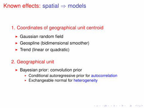
Known effects: spatial⇒ models

1. Coordinates of geographical unit centroid

I Gaussian random fieldI Geospline (bidimensional smoother)I Trend (linear or quadratic)

2. Geographical unit

I Bayesian prior: convolution priorI Conditional autoregressive prior for autocorrelationI Exchangeable normal for heterogeneity

Known effects (?): interactions

⇒ complexity of cancer aetiology

I Interaction age-period and/or cohort effectI P-spline or indicator variable for cohort effectI Smoothed age-period surface (tensor product)

I Gender-period and gender-ageI Varying coefficients model (VCM):

f1(t)+ s× f2(t)

f1(t) is the basal time effect (for s = 0) and f2(t) is the addedtime effect for s = 1

I Temporal slope and intercept by genderI Space-period, age-space-period and gender-space-period:

VCM or multidimensional smoother

Outline

I Cancer registriesI Dataset and analyses aimsI Known effectsI Our dataI Works in progress and problems

Our data: dataset

I ENT data: ear-nose-throat cancerI Alcohol and tobacco consumptionI Latency between exposure and cancer

I Covariates:I Gender: 0 for female and 1 for maleI Age into 9 groups: [0-45 years), 5-year intervals and [80 or

more]I Time: date of diagnosis categorized in year, from 1988 to

2005I Geographical unit of residence, with centroid coordinates

I Population countsI 1990 census for 1988 to 1991I 1999 census for 1998 to 2002I Linear interpolation at 1993 and 1996 for 1992-1994 and for

1995-1997I 2005 census for 2003 to 2005

I Adjusted risk on gender

Our data: objectives

I Compare models for detecting effects of time, space, sexand/or interactions

I Space-time trend and interactionI Account for covariates with possible non linear effects,

such as ageI Models are compared using the AIC criterion

Analyses carried out using packages mgcv and geoR for R

Our data: exploratory analysisI Total number of cases: 3,850, 87% male

Figure: Raw SIRs (with 95% CI) by year and gender

Our data: exploratory analysis

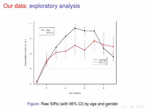
Figure: Raw SIRs (with 95% CI) by age and gender

Our data: exploratory analysis

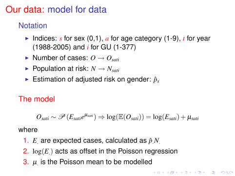
Our data: model for data

NotationI Indices: s for sex (0,1), a for age category (1-9), t for year

(1988-2005) and i for GU (1-377)I Number of cases: O→ Osati

I Population at risk: N → Nsati

I Estimation of adjusted risk on gender: ps

The model

Osati ∼P (Esatieµsati)⇒ log(E(Osati)) = log(Esati)+ µsati

where1. E. are expected cases, calculated as p.N.

2. log(E.) acts as offset in the Poisson regression3. µ. is the Poisson mean to be modelled

Our data: our spatiotemporal models

Osati ∼P (Esatieµsati)

1. Models for age, time and genderModel µ =M00 f1(a) Cubic P-spline for age (9 knots)M01 f1(a)+ sβs + tβt + stβst Fixed main effects and interactionM02 f1(a)+ f2(t) Cubic P-spline for year (18 knots)M03 f1(a, t) Tensor product (9 and 18 knots)M04 f1(a)+ sβs + f2(t) Cubic P-spline for year (18 knots)

and fixed effect for genderM05 f1(a)+ s× f2(t) VCM model

Our data: our spatiotemporal models

Osati ∼P (Esatieµsati)

2. Models for space and timeModel µ =M00 f1(a) Cubic P-spline for age (9 knots)M02 f1(a)+ f2(t) Cubic P-spline for year (18 knots)M11 f1(a)+ f3(X,Y) Tensor product (thin plate spline)M12 f1(a)+ f2(t)+ f3(X,Y) M02+M11M13 f1(a)+ f4(X,Y, t) Tensor product (thin plate spline

for space and cubic spline for year)

Our data: models results

1. Models for age, time and gender

Model µ = AIC R2 edff (a) f (t)

M00 f1(a) 22,189 0.444 7.745M01 f1(a)+ sβs + tβt + stβst 22,014 0.467 7.753M02 f1(a)+ f2(t) 22,041 0.463 7.754 7.162M03 f1(a, t) 22,159 0.456 20.000M04 f1(a)+ sβs + f2(t) 22,037 0.465 7.754 7.170M05 f1(a)+ s× f2(t) 21,998 0.467 7.754 F: 1.007

M: 7.191

Our data: models resultsI Cohort effect views as an age-time smoothed surface

(type="response")

Our data: models results

2. Models for space and time

Model µ = AIC R2 edff (a) f (t) f (X,Y)

M00 f1(a) 22,189 0.444 7.745M02 f1(a)+ f2(t) 22,041 0.463 7.754 7.162M11 f1(a)+ f3(X,Y) 22,157 0.449 7.772 9.630M12 f1(a)+ f2(t)+ 22,010 0.470 7.783 7.136 9.490

+f3(X,Y)M13 f1(a)+ f4(X,Y, t) Memory crashes

Our data: models results

3. Model for age, gender, time and space

Model µ = AIC R2 edff (a) f (t) f (X,Y)

M05 f1(a)+ s× f2(t) 21,998 0.467 7.754 F: 1.007M: 7.191

M12 f1(a)+ f2(t)+ 22,010 0.470 7.783 7.136 9.490+f3(X,Y)

M20 f1(a)+ f3(X,Y) 21,967 0.473 7.760 F: 1.006 9.390+s× f2(t) M: 7.182

Our data: results model M20

Parametric coefficients:Estimate Std. Error z value Pr(> |z|)

(Intercept) 0.47648 0.01863 25.57 <2e-16 ***—Approximate significance of smooth terms:

edf Ref.df Chi.sq p-values(age) 7.760 7.760 23637.01 < 2e-16 ***te(X,Y) 9.390 9.390 328.31 < 2e-16 ***s(an):sex 1.006 1.006 16.06 6.21e-05 ***s(an):sex2 7.182 7.182 1509.61 < 2e-16 ***—R-sq.(adj) = 0.473 Deviance explained = 27.9%UBRE score = -0.87008 Scale est. = 1 n = 122148

Our data: results⇒ age effect

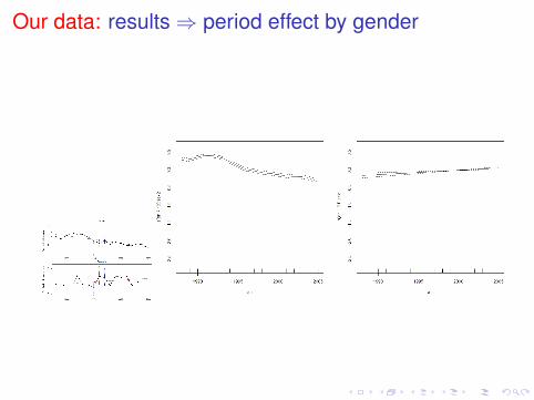
Our data: results⇒ period effect by gender

Our data: results⇒ spatial effect

Our data: results⇒ spatial effect

I Empirical semi-variogram of Pearson residuals for 1988,1996 and 2005

Our data: conclusions

I First comprehensive analysisI GAMs provide framework for spatio-temporal modeling tool

of different natureI to estimate space-time trends with confidence bandsI the model allows to address scientific questions through the

inclusion of covariates

Outline

I Cancer registriesI Dataset and analyses aimsI Known effectsI Our dataI Works in progress and problems

Works in progress and problems

I Better handling of memory in RI Models comparisons

I Likelihood ratio test⇒ nested modelsI Penalized likelihood like AIC or BIC⇒ same data

1. Model with age effect: data aggregated on all variablesexcept age

2. Model with age and sex effects: data aggregated on allvariables except age and sex⇒ two times bigger dataset

Works in progress: ZIP models

Due to covariates, the ENT dataset counts were spread over122,148 cells with 119,324 empty cells (97%)

I Higher incidence of zeros than expected under Poissondistribution⇒ zero-inflated Poisson distribution

Pr(O,µ,ω) =

{ω +(1−ω)e−µ if O = 0(1−ω)e−µ µO

O! if O > 0

I Variance is two times mean (0.070/0.032)⇒ moreappropriate distributions: quasipoisson, negativebinomiale, Tweedie

Works in progress: multivariate analyses

The problem

I ENT and lung cancers share common risk factors→ No individual measure of consumption→ Use geographical unit for proxy (ecological bias)I Specific risk factor for ENT cancer?

An ideaI Use SIR for lung cancer as covariateI Estimation of a VCM: I(SIRlung > 1)× fspat(X,Y)

Works in progress: multivariate analyses

A second (and better) idea

I Multivariate approachI A model

Osati ∼P(Esatieµsati

)where

log

(O(1)

sati

O(2)sati

)= log

(E(1)

sati

E(2)sati

)+ f1(a)+ · · ·+

(f (1)(X,Y)f (2)(X,Y)

)I Bayesian models (shared components)

Works in progress: more complex correlation structure

Time effect

Osati ∼P (Esatieµsati)⇒ log(Osati) = log(Osati)+ µsati + εsati

where ε ∼ N(0,Λ) and covariance matrix Λ modelled as a firstorder autoregressive (AR1) process on time

I Memory problems

Spatial effect

I Mimic an autocorrelation like in convolution prior modelI Replace thin plate splines with a "kriging component"⇒

memory problem

Works in progress

Monotonic splines on time and spatial effects!!!

Thank you for your attention