Spatiotemporal dynamics of methane emission from ricefields at global scale

Amit Chakraborty a,*, Dilip Kumar Bhattacharya b, Bai-Lian Li a

aEcological Complexity and Modeling Laboratory, Department of Botany and Plant Sciences, University of California,

Riverside, CA 92521-0124, USAbDepartment of Pure Mathematics, University of Calcutta, 35, Ballygange Circular Road, Kolkata 19, West Bengal, India

e c o l o g i c a l c o m p l e x i t y 3 ( 2 0 0 6 ) 2 3 1 – 2 4 0

a r t i c l e i n f o

Article history:

Received 20 January 2006

Received in revised form

19 May 2006

Accepted 25 May 2006

Published on line 18 July 2006

Keywords:

Spatiotemporal dynamics

Spatiotemporal domain

Biogeochemical process

Monod type-1 kinetics

Monod type-2 kinetics

Brouwer’s fixed point theorem

a b s t r a c t

Rice fields are one of the anthropogenic sources of methane emission with largest uncer-

tainty. Precise global estimation from different sites is difficult due to large spatial and

temporal variabilities in climate, soil properties, duration and pattern of flooding, rice

cultivars and crop growth, organic amendments, fertilization, and cultural practices. The

temporal dynamics of methane emission from rice fields represented by ordinary differ-

ential equations is coupled with its spatial dynamics by connecting the temporal methane

emission model with soil–climate model. This model includes detailed biogeochemical

processes of methane emission, which is capable to identify emission sources and can be

used to address the natural/artificial control and feedback issues. A complete computational

scheme for identifying out-busting emission sources and for simulating and reducing

methane emission from rice fields has been proposed in this paper with respect to space

and time.

# 2006 Elsevier B.V. All rights reserved.

avai lab le at www.sc iencedi rect .com

journal homepage: ht tp : / /www.e lsev ier .com/ locate /ecocom

1. Introduction

Precise global estimation of methane emission has been

difficult due to large spatial and temporal variability in

methane measured at different sites which are different in

climate, soil properties, duration and pattern of flooding, rice

cultivars, crop growth, organic amendments, fertilization and

cultural practices (Matthews et al., 2000). An emission model,

which includes the oxidation of produced methane, developed

by Chakraborty and Bhattacharya (2006a,b), is capable to

explain the temporal variability of methane emission through

oxidation. Several dynamical regimes have formed through

qualitative analysis of the Chakraborty and Bhattacharya’s

model and corresponding dynamic features have been

interpreted through emission indices (Chakraborty and

Bhattacharya, 2006a). But spatial variability of emission has

* Corresponding author. Tel.: +1 951 827 4776; fax: +1 951 827 4437.E-mail address: amitc@ucr.edu (A. Chakraborty).

1476-945X/$ – see front matter # 2006 Elsevier B.V. All rights reservedoi:10.1016/j.ecocom.2006.05.003

not been considered in that model. Matthews et al. (2000) have

tried to incorporate spatial information of climate, soil

properties, cultural practices, fertilization with mechanistic

model of methane fluxes in Geographical Information System

(GIS) environment. But their actual motivation towards the

development of the MERES (Methane Emission in Rice

Ecosystems) model was to simulate methane emission from

rice fields. They did not discuss the stability and control issues

of the spatiotemporal process of methane emission analyti-

cally. The approaches in determining trace gas emission

sources with respect to space and time as described by Liu

(1996) can be classified into three broad categories. One of

these is the flux extrapolation method. Emission flux

measurements made at individual sites are extrapolated to

larger scales using mapping procedures to obtain the region for

global emissions. Because available in situ flux measurements

d.

e c o l o g i c a l c o m p l e x i t y 3 ( 2 0 0 6 ) 2 3 1 – 2 4 0232

are geographically very sparse at global scale, large uncertain-

ties must be involved in the estimates obtained using this flux

extrapolationmethod.Another approach is the inversemethod;

it involves the use of an atmospheric chemical transport model.

The model predicted concentrations are compared with the

observed concentrations of trace gases. This is to determine by

optimal estimation procedures, what distribution of sources

best fits the observations. Inverse method studies using 2D

(Cunnold et al., 1983, 1986; Prinn et al., 1990) and 3D CTM’s

(Chemical transport model) (Hartley and Prinn, 1993) have

shown the great potential of this approach for determining the

global surface sources of trace gases. However, the imperfect

atmospheric circulation in current CTMs places limitations on

the current use of the inverse method. Specifically for

estimating regional emissions, the inverse method involves

large uncertainties (Hartley and Prinn, 1993; Mahowald, 1996).

Both the extrapolation method and the inverse method do not

enlighten us about the processes, which are primarily respon-

sible for the trace gas emissions. They are able to quantify the

current state but are not capable of addressing issues like the

emission related feedbacks. A third approach involves process-

oriented models. If such models are good at simulating trace gas

emissions at individual sites, they may be a powerful tool for

estimating regional and global emissions of the trace gases. For

the latter estimation we need to know the global distribution of

the controlling parameters and for assessing the feedbacks, we

need to connect the emission processes with climate processes.

The use of process-oriented models without considering

horizontal interactions (e.g. horizontal heat and moisture flows

in a soil model) could be categorized as an extrapolation

method. However a process-oriented model does not use a

simple extrapolation of the relevant variables (e.g. the flux). It is

therefore useful to distinguish this method from the extra-

polation method. Because a process-oriented model is based on

an understanding of the biogeochemistry of the trace gas

production, the approach using a process-oriented model to

estimate the global emissions does not omit explicit connec-

tions to the flux driving variables. These are unavoidable in

simply extrapolating the measured flux to the whole globe.

There are global models which attempt to simulate methane

emission spatiotemporarily by considering a variety of complex

regulating parameters. Bartlett and Harriss (1993) have done an

excellent review on wetland methane emissions using an

arbitrary assumption about methane emission by season

similar to that used in Fung et al. (1991). In this paper we follow

third approach as stated above.

The methane emission process is a composition of several

microbacterial kinetics. In particular, rice field soils, character-

ized by O2 depletion, high moisture and relatively high organic

substrate levels, offer an ideal environment for the activity of

methanogenic bacteria, a group of methane producing bacteria

and are one of the major anthropogenic methane emission

sources (Matthews et al., 2000). Basically two distinct micro-

biological processes control methane emission from rice fields,

methane production, a microbiological anaerobic process

responsible for methane production and methane oxidation,

a microbiological but aerobic process responsible for methane

oxidation. The methane emission from rice fields is the net

result of opposing bacterial processes; methane production and

methane oxidation, both of which can be found side by side in

floodedrice soils (Neue and Boonjwat,1993).A considerable part

of produced methane is oxidized microbiologically. Oremland

and Culbertson (1992) found that methanotropic bacteria

consumed more than 90% of produced methane in aerobic

environment. The part of produced methane which is not

oxidized enters into atmosphere. Soil–climate, primarily soil

temperature and soil moisture/water content are known to play

a strong role in the emission process. The metabolic activity of

soil microbes, methanogen, methane producing bacteria,

methanotrop, methane oxidizing bacteria and also the

microbes in the decomposition chain that produce substrates

for the methanogen from soil organic matter are strongly

temperature dependent. Soil moisture status controls the

oxygen availability for methanotropic bacteria, which consume

methane under aerobic conditions. But both the soil-climatic

variables soil temperature and soil moisture, which are driven

by surface climate, are having both temporal as well as spatial

variabilities even in very small spatial scale. It makes the

methane emission process spatiotemporal in nature.

Our major objective in this paper is to combine spatial

variability of methane emission with temporal one. A process-

based temporal model on methane emission developed by

Chakraborty and Bhattacharya (2006a,b) has been extended to

global spatial scale by connecting it with climate model. The

advantage of using spatially extended methane emission

model, i.e. spatiotemporal model of methane emission, is that

it includes detailed biogeochemical processes of methane

emission and is capable to explain process stability. Therefore,

it can be used to address the natural and artificial control and

feedback issues.

2. Spatiotemporal model

The methane emission model developed by Chakraborty and

Bhattacharya (2006a,b) is considered to include the temporal

dynamics of methane emission. The model includes detailed

biochemical processes of methane emission, i.e. process-

based. There are four different microbacterial kinetics

involved in this model. Monod type-1 kinetics is used to

describe biomass degradation and associated substrate for-

mation. Monod type-2 kinetics is used to describe methano-

genic bacterial kinetics through which substrate degraded to

form methane. Acidogenic bacterial kinetics is accommodated

in the model in approximated linearized form. Modified

Monod equation is used to include methanotropic bacterial

kinetics responsible for methane oxidation. The biomass

growth in open environment is considered in the form of

logistic (S-curve) equation. The model is given below:

dBdt¼ MB 1� B

K

� �� Bmax

BKB þ B

� �S

dSdt¼ Y Bmax

BKB þ B

� �S

� �� aS� Smax

S2

ðKc þ SÞðKd þ SÞX

dXdt¼ Z Smax

S2

ðKc þ SÞðKd þ SÞX" #

�OXX

Xþ KCH4

; 0<Y<1; 0<Z< 1

8>>>>>>>>>>>>><>>>>>>>>>>>>>:where B is the biomass concentration, S the substrate con-

centration, X the methane concentration, t the time, M the

ðLipidÞNeutralfat ! Long chain fatty acids

e c o l o g i c a l c o m p l e x i t y 3 ( 2 0 0 6 ) 2 3 1 – 2 4 0 233

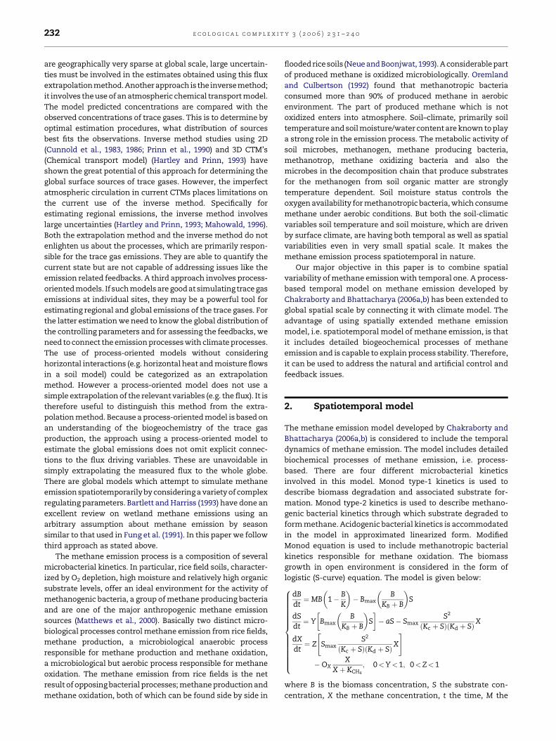
Fig. 1 – The form of g(us) described by Godwin and Jones

(1991).

specific growth rate of B, K the environmental carrying capa-

city, Bmax the maximum biomass utilization rate, KB the half

saturation coefficient, Y the yield coefficient, a the endogenous

decay rate of substrate, Smax the maximum substrate utiliza-

tion rate, Kc and Kd are the saturation coefficients in Monod

type-2 kinetics, Z the yield coefficient, OX the methane oxida-

tion rate and KCH4 is the half saturation constant.

Now we connect the temporal model (1) with climate

model. The approach we follow for connecting the climate

model with temporal model is written in following steps:

Step 1: We identify microbacterial kinetics parameters of the

temporal model (1) those are heavily influenced by soil

climate. We call them spatiotemporal parameters of the model.

Step 2: We form equations of all identified parameters,

represent their dependence on soil-climatic variables.

Step 3: We consider known equations of soil-climatic

variables represent their spatiotemporal variability on

plane surface.

The effects of soil depth in the variability of soil-climatic

variables are not considered in this paper.

2.1. Spatiotemporal parameters and their dependenceequations

The availability of favorable substrates for methane producing

bacteria (the methanogen) directly depends on biomass

utilization rate due to microbacterial activities. In the model

(1), biomass utilization rate is represented by Monod type-1

kinetics. The parameter Bmax, in Monod type-1 kinetics controls

the microbacterial activity. Topiwala and Sinclair (1971)

introducedthe expression for Bmax asa functionof temperature,

i.e. Bmax(T). They investigated the relationship between kinetic

coefficients and temperature on the basis of experimental

results by pure culture of Aerobactor aerogens and reported that

Bmax is dependent on temperature. Chen et al. (1980) and

Hashimoto (1982) show that temperature influenced the

coefficient Bmax, of the Monod type model when beef cattle

manure is applied to the anaerobic digestion process in the

temperature range of 35–65 8C. Novak (1974) suggested that the

effect of temperature on the kinetic coefficients in the Monod

type model could be estimated in the following manner:

BmaxðTÞ ¼ BmaxðT0Þexpfc1ðT� T0Þg

where Bmax(T) = Bmax at temperature T (8C), Bmax(T0) = Bmax at

reference temperature T0 (8C). c1 = constant = the slope of

ln(Bmax(T)) versus temperature line.

In MERES model (Matthews et al., 2000), the rate of decay of

soil organic matter limited by soil temperature, soil moisture

and C/N of decaying material was calculated as

dOp

dt¼ OpRpðmaxÞ fðTsÞgðusÞhðksÞ

where Op (kg ha�1) is the amount of organic matter remaining

in the pool p 2 {carbohydrate, cellulose, and lignin} on the day

in question, and f(Ts), g(us), h(ks) are dimensionless multipliers

for soil temperature (Ts, 8C), soil moisture (us, m3 water m�3

soil), and the pool C/N (ks, kg C kg�1 N), respectively. The form

of g(us) described by Godwin and Jones (1991) is shown in Fig. 1.

It can be seen that decomposition rates in flooded soils (us = u-

sat) are about half those in moist but well drained soils.

We consider here a fixed range of soil temperature and soil

water content, i.e. TB0 < T < TB1 and WB0 < W < WB1 within

which the microbial activities enhance the biomass utilization

process. Therefore, the kinetic parameter, Bmax is positive

within the considered range and it gradually increases up to

maximum limit as soil temperature, T and soil water content,

W gradually increases. After that it starts to decrease with

respect to T and W. Hence we can express Bmax as given below:

Bmax ¼ q1ðT� TB0ÞðW �WB0Þ 1� TTB1

� �1� W

WB1

� �(2)

where q1 is the proportionality constant. Different values of q1

can be derived by experiments for different soil types. The

expression for KB is considered as suggested by Novak (1974) is

given below:

KBðTÞ ¼ u expf�CðT� TB0Þg (3)

where u is the microbial kinetic constant in Monod type-1

kinetics that can be derived from experiment and C = con-

stant = ln(KB(T)) versus temperature line.

A group of acidogenic bacteria includes various kinds of

bacteria, which ferment organic matter/complex materials

and produce organic acids in anaerobic conditions. The

distribution of favorable substrate for methanogenesis

depends on the species of acidogenic bacteria and on the

environmental conditions such as soil water content and soil

temperature. Amino acids are derived from protein and are

degraded by Clostridium species (Siebelt and Toerien, 1969)

mainly via stickland reaction (Nagase and Matsuo, 1982).

Degradation of carbohydrate, proteins and lipids by acidogenic

bacteria are summarized below:

ðCarbohydrateÞPolysaccharide ! Monosaccharide

ðProteinÞProtein ! Aminoacids

e c o l o g i c a l c o m p l e x i t y 3 ( 2 0 0 6 ) 2 3 1 – 2 4 0234

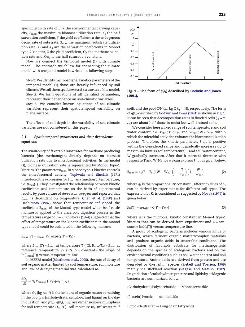
Fig. 2 – Average values of glucose concentration with

respect to temperature.

‘!’ indicates reaction conducted by acidogenic bacteria. Endo

et al. (1983) carried out continuous experiments on the effects of

temperature on the acidogenic phase using an anaerobic che-

mostat reactor with glucose as a main substrate, retention time

of 1 day and temperature ranging from 5 to 60 8C at intervals of

5 8C. Fig. 2 shows average values of glucose concentration with

respect to temperature. The growth rate of acidogenic bacteria

has a maximum at 30 8C and total organic acid production rate

has maximum at 35 8C. After the temperature of 45 8C, the rate

of microbial growth begins to decrease.

In the model (1) acidogenic bacterial kinetics is considered

in approximated linearized form (Chakraborty and Bhatta-

charya, 2006b). In the model (1), ‘a’ is the acidogenic bacterial

kinetics parameter expresses the acidogenic bacterial activity.

From the above discussion, it is clear that the parameter ‘a’ is

temperature dependent and the dependence equation can be

formed like S-curve. The equation for ‘a’ is given below:

a ¼ q2ðT� Ta0Þ 1� TTa1

� �(4)

where q2 is the acidogenic bacterial kinetic constant and the

soil temperature, T lies between Ta0 and Ta1, i.e. Ta0 < T < Ta1

within which acidogenic bacteria are active.

In Monod kinetics, saturation coefficients but not max-

imum specific growth rate are affected by soil temperature in

methanogenesis from acetate according to Lawrence and

McCarty (1969). The equations are as follows:

logKSðTm2ÞKSðTm1Þ

� �¼ 6980

1Tm2� 1

Tm1

� �or

lnKSðTm2ÞKSðTm1Þ

� �¼ 6980

1Tm2� 1

Tm1

� �

where KS(Tm1) and KS(Tm2) are KS values at temperature T0m1K

and T0m2K, respectively, and KS is the saturation coefficient.

O’Rourke (1968) made an experiment in the temperature range

of 20–30 8C and described the effects of temperature in degra-

dation of lipid in sewage by following equations:

S ¼ 6:67� 100:015ðT�35Þ ðd�1Þ:

max

For our purpose, we consider equation for Smax like

O’Rourke’s experimentally derived equation and expressions

for Kc and Kd as described by Lawrence and McCarty (1969). The

equations are given below:

Smax ¼ u1 expfC1ðT� Tm0Þg (5)

lnKcðTÞ

KcðTm0Þ

� �¼ u2

1T� 1

Tm0

� �(6)

lnKdðTÞ

KdðTm0Þ

� �¼ u3

1T� 1

Tm0

� �(7)

where u1, u2 and u3 are methanogenic bacterial kinetics con-

stants can be derived from experiment and C1 = constant = the

slope of In(Smax(T)) versus temperature line. The soil tempera-

ture, T lies between Tm0 and Tm1, i.e. Tm0 < T < Tm1 within

which methanogenic bacteria are active.

Microbiological oxidation of methane is carried out by

methanotropic bacteria, which are present in small numbers

in most of the soils. Long-term exposures of soils to high levels

of methane result in the growth of populations of methano-

tropic bacteria with high capacity of methane oxidation.

Increasing percolation rates of water may supply sufficient

oxygen to soil to raise Eh (soil redox potential), decrease

methane production and increase methane oxidation. Stein

et al. (2001) have considered the effects of soil O2 concentra-

tion using modified Monod equation. As described in Stein’s

model the rate of oxidation, OX, due to the activity of

methanotropic bacteria depends on soil O2 concentration by

the equation, is given below:

OX ¼ VmaxCO2

CO2 þ KO2

where Vmax is the maximum methane oxidation rate, CO2the

soil O2 concentration and KO2is the half saturation constant.

It is well known that soil O2 concentration is inversely

proportional to soil water content. In the above expression, CO2

can be replaced by ( p(1/W)) where p is the proportionality

constant and it varies with respect to soil types. Therefore, the

above expression becomes as follows:

OX ¼ Vmaxp

pþWKO2

: (8)

2.2. Spatiotemporal variation of soil temperature

The standard instationary heat flow equation for soils has been

considered here (Huwe, 1997). The equation is given below:

@T@t¼ k1r02ðTÞ � k2rðTÞ (9)

where T is the soil temperature

k1 ¼l

cv; k2 ¼

cvwqw

cv

r� @

@xþ @

@y; r0 � @2

@x2þ @2

@y2

where cv is the volumetric heat capacity, l the volumetric heat

conductivity, cvw the volumetric heat capacity of water and qw

is the water flux.

Note: Volumetric heat capacity is the amount of heat

required to raise the temperature of unit volume by 18 (8K or 8C).

e c o l o g i c a l c o m p l e x i t y 3 ( 2 0 0 6 ) 2 3 1 – 2 4 0 235

2.3. Spatiotemporal variation of soil water content

The general equation of soil water flow (Q) can be written as:

Q = �k5h where k is the hydraulic conductivity and h is the

hydraulic head. Let W be soil water content which is measured

by a fraction of soil pore space (0 �W � 1). Then soil water

balance equation is given below:

@W@t¼ 1

nrQ ¼ 1

nrð�krhÞ ¼ �1

n

� �rðkrhÞ

where n is the soil porosity.

Hydraulic conductivity (k) and hydraulic head (h) depend

on soil water parameter and soil water content itself. They

are described below as suggested by Clapp and Hornberger

(1978):

k ¼ ksatW2bþ3; h ¼ ’satW

�b

where ksat is the saturated hydraulic conductivity, b the soil

water parameter and wsat is the water tension parameter.

Therefore,

@W@t¼ �1

n

� �ksat’satrðW2bþ3rW�bÞ:

Now, we have

rðW2bþ3rW�bÞ ¼ ð�bÞðbþ 2ÞWbþ1ðrWÞ2 þ ð�bÞWbþ2r02W;

i.e.

@W@t¼ bksat’satðbþ 2Þ

n

� �Wbþ1ðrWÞ2 þ bksat’sat

nWbþ2r02W:

Hence

@W@t¼ c1Wbþ1ðrWÞ2 þ c2Wbþ2r02W (10)

where

c1 ¼b’satksatðbþ 2Þ

n; c2 ¼

bksat’sat

n:

2.4. Spatiotemporal system

The model (1) combines with all dependence Eqs. (2)–(8) of all

identified spatiotemporal parameters and differential Eqs. (9)

and (10) of T and W described above form the spatiotemporal

model of methane emission from rice fields.

The rainfall is assumed to directly add water to soil without

considering the ‘interception effect’ of the overlying vegetation

orother bypass effect. Values of n, ksat,bandwsat entirely depend

on soil types (DeVries, 1975; Clapp and Hornberger, 1978).

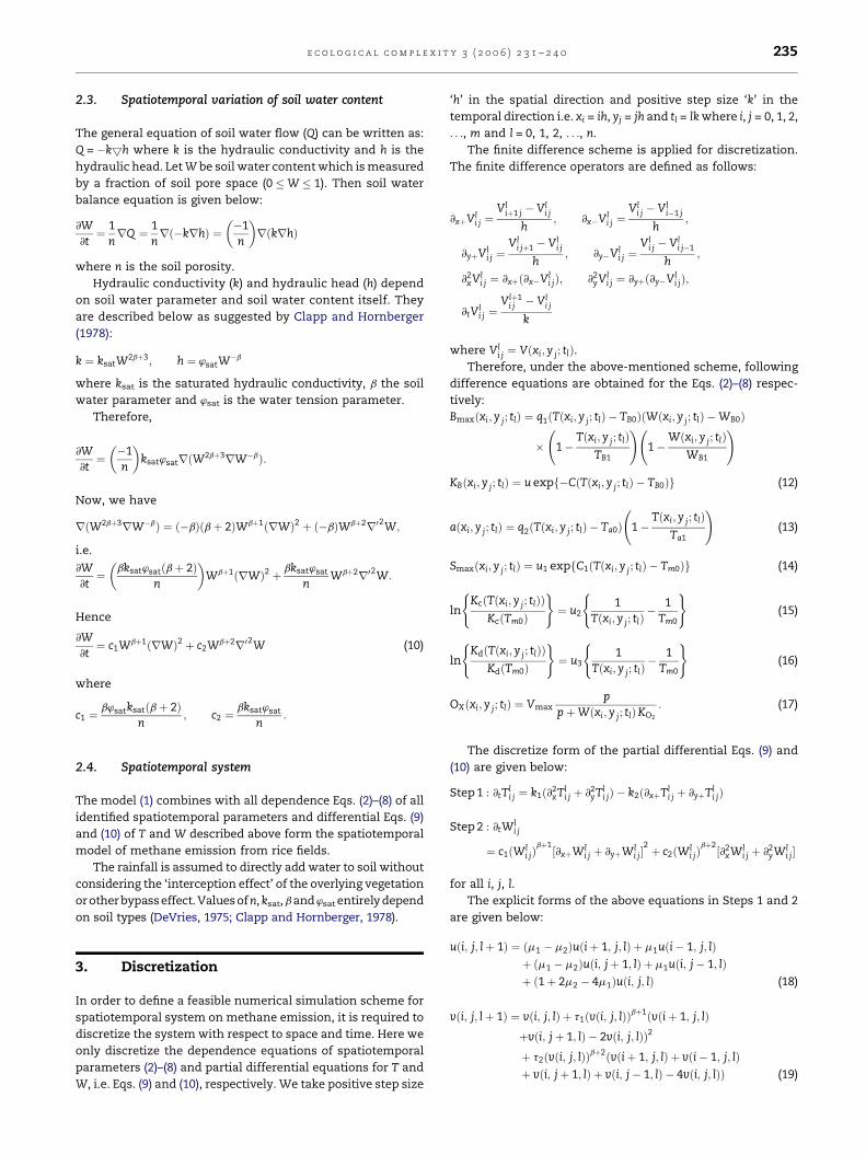
þ vði; jþ 1; lÞ þ vði; j� 1; lÞ � 4vði; j; lÞÞ (19)

3. Discretization

In order to define a feasible numerical simulation scheme for

spatiotemporal system on methane emission, it is required to

discretize the system with respect to space and time. Here we

only discretize the dependence equations of spatiotemporal

parameters (2)–(8) and partial differential equations for T and

W, i.e. Eqs. (9) and (10), respectively. We take positive step size

‘h’ in the spatial direction and positive step size ‘k’ in the

temporal direction i.e. xi = ih, yj = jh and tl = lk where i, j = 0, 1, 2,

. . ., m and l = 0, 1, 2, . . ., n.

The finite difference scheme is applied for discretization.

The finite difference operators are defined as follows:

@xþVli j ¼

Vliþ1 j � Vl

i j

h; @x�Vl

i j ¼Vl

i j � Vli�1 j

h;

@yþVli j ¼

Vli jþ1 � Vl

i j

h; @y�Vl

i j ¼Vl

i j � Vli j�1

h;

@2xVl

i j ¼ @xþð@x�Vli jÞ; @2

yVli j ¼ @yþð@y�Vl

i jÞ;

@tVli j ¼

Vlþ1i j � Vl

i j

k

where Vli j ¼ Vðxi; y j; tlÞ.

Therefore, under the above-mentioned scheme, following

difference equations are obtained for the Eqs. (2)–(8) respec-

tively:

Bmaxðxi; y j; tlÞ ¼ q1ðTðxi; y j; tlÞ � TB0ÞðWðxi; y j; tlÞ �WB0Þ

� 1�Tðxi; y j; tlÞ

TB1

!1�

Wðxi; y j; tlÞWB1

!

KBðxi; y j; tlÞ ¼ u expf�CðTðxi; y j; tlÞ � TB0Þg (12)

aðxi; y j; tlÞ ¼ q2ðTðxi; y j; tlÞ � Ta0Þ 1�Tðxi; y j; tlÞ

Ta1

!(13)

Smaxðxi; y j; tlÞ ¼ u1 expfC1ðTðxi; y j; tlÞ � Tm0Þg (14)

lnKcðTðxi; y j; tlÞÞ

KcðTm0Þ

( )¼ u2

1Tðxi; y j; tlÞ

� 1Tm0

( )(15)

lnKdðTðxi; y j; tlÞÞ

KdðTm0Þ

( )¼ u3

1Tðxi; y j; tlÞ

� 1Tm0

( )(16)

OXðxi; y j; tlÞ ¼ Vmaxp

pþWðxi; y j; tlÞKO2

: (17)

The discretize form of the partial differential Eqs. (9) and

(10) are given below:

Step 1 : @tTli j ¼ k1ð@2

xTli j þ @2

yTli jÞ � k2ð@xþTl

i j þ @yþTli jÞ

Step 2 : @tWli j

¼ c1ðWli jÞ

bþ1½@xþWli j þ @yþWl

i j�2 þ c2ðWl

i jÞbþ2½@2

xWli j þ @2

yWli j�

for all i, j, l.

The explicit forms of the above equations in Steps 1 and 2

are given below:

uði; j; lþ 1Þ ¼ ðm1 � m2Þuðiþ 1; j; lÞ þ m1uði� 1; j; lÞþ ðm1 � m2Þuði; jþ 1; lÞ þ m1uði; j� 1; lÞþ ð1þ 2m2 � 4m1Þuði; j; lÞ (18)

vði; j; lþ 1Þ ¼ vði; j; lÞ þ t1ðvði; j; lÞÞbþ1ðvðiþ 1; j; lÞþvði; jþ 1; lÞ � 2vði; j; lÞÞ2

þ t2ðvði; j; lÞÞbþ2ðvðiþ 1; j; lÞ þ vði� 1; j; lÞ

e c o l o g i c a l c o m p l e x i t y 3 ( 2 0 0 6 ) 2 3 1 – 2 4 0236

where

uði; j; lÞ ¼ Tðxi; y j; tlÞ; vði; j; lÞ ¼Wðxi; y j; tlÞ; m1 ¼kk1

h2;

m2 ¼kk2

h; t1 ¼

kc1

h2; t2 ¼

kc2

h2:

From now onwards we consider the discretized spatio-

temporal system, i.e. the model (1) combine with Eqs. (11)–(19).

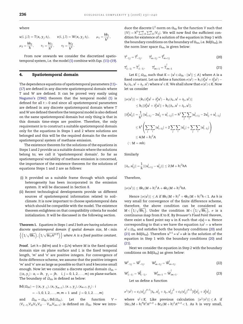
4. Spatiotemporal domain

The dependence equations of spatiotemporal parameters (11)–

(17) are defined in any discrete spatiotemporal domain where

T and W are defined. It can be proved very easily using

Nagumo’s (1942) theorem that the temporal model (1) is

defined for all t > 0 and since all spatiotemporal parameters

are defined in any discrete spatiotemporal domain where T

and W are defined therefore the temporal model is also defined

on the same spatiotemporal domain but only thing is that in

this domain time-steps are positive. Therefore, the only

requirement is to construct a suitable spatiotemporal domain

only for the equations in Steps 1 and 2 where solutions are

belonged and this will be the required domain for the entire

spatiotemporal system of methane emission.

The existence theorem for the solutions of the equations in

Steps 1 and 2 provide us a suitable domain where the solutions

belong to; we call it ‘spatiotemporal domain’. So far as

spatiotemporal variability of methane emission is concerned,

the importance of the existence theorem for the solutions of

equations Steps 1 and 2 are as follows:

(i) It

provided us a suitable frame through which spatial

heterogeneity has been incorporated in the emission

system. It will be discussed in Section 8.

(ii) R

ecent technological developments provide us different

sources of spatiotemporal information related to soil–

climate. It is now important to choose spatiotemporal data

which should be compatible with the model. The existence

theorem enlightens on that compatibility criteria for model

initialization. It will be discussed in the following section.

Theorem1. Equations in Steps 1 and 2 both are having solutions on

discrete spatiotemporal domain if spatial domain size, M<min

1=ffiffiffiffiffiffiffiffi8k1

p� ; 1=

ffiffiffiffiffiffiffiffiffiffiffiffiffiffiffiffiffiffi8c2Abþ2

p� n owhere A is a fixed positive constant.

Proof. Let h = (M/m) and k = (L/n) where M is the fixed spatial

domain size on plane surface and L is the fixed temporal

length, ‘m’ and ‘n’ are positive integers. For convergence of

finite difference scheme, we assume that the positive integers

‘m’ and ‘n’ are as large as possible so that h and k become small

enough. Now let we consider a discrete spatial domain Vhh ¼fðxi; y jÞ : xi ¼ ih; y j ¼ jh; i; j ¼ 0; 1; 2; . . . ;mg on plane surface.

The boundary of Vhh is defined as below:

BdðVhhÞ ¼ fðxi; y�1Þ; ðxi; ymþ1Þ; ðx�1; y jÞ; ðxmþ1; y jÞ : i

¼ �1; 0;1;2; . . . ;m;mþ 1 and j ¼ 0;1;2 . . . ;mg

and Vhh ¼ Vhh [BdðVhhÞ. Let the function V ¼ðVið�1ÞVi0Vi1Vi2 � � �VimVimþ1Þ is defined on Vhh. Now we intro-

duce the discrete L2-norm on Vhh for the function V such that

jjVjj ¼ h4Pmj¼0

Pmi¼0 jVi jj. We will now find the sufficient con-

dition for existence of a solution of the equation in Step 1 with

the boundary conditions on the boundary of Vhh, i.e. Bd(Vhh), in

the norm liner space Vhh, is given below:

Tl�1 j ¼ T

l�1 j; Tl

mþ1 j ¼ Tlmþ1 j (20)

Tlið�1Þ ¼ T

_ lið�1Þ; Tl

imþ1 ¼ T^l

imþ1 (21)

Let K�Vhh, such that K ¼ ful 2Vhh : jjuljj � Ag where A is a

fixed constant. Let us define a function sðulÞ ¼ k1ð@2xul þ @2

yulÞ �k2ð@xþul þ @yþulÞwhere ul 2K. We shall show that sðulÞ 2K. Now

let us consider

jjsðulÞjj ¼ jjk1ð@2xul þ @2

yulÞ � k2ð@xþul þ @yþulÞjj

� k1jj@2xul þ @2

yuljj þ k2jj@xþul þ @yþuljj:

jj@2xul

i jjj ¼1

h2jjul

iþ1 j � 2uli j þ ul

i�1 jjj ¼ h2X

j

Xi

juliþ1 j � 2ul

i j þ uli�1 jj

� h2X

j

Xi

juliþ1 jj þ 2

Xj

Xi

juli jj þ

Xj

Xi

juli�1 jj

0@

1A

� 4ðMþ hÞ2A

ð{ M ¼ mhÞ

Similarly

jj@xþuli jjj ¼

1hjjðul

iþ1 j � uli jÞjj � 2ðMþ hÞ2hA

Therefore,

jjsðulÞjj � 8k1ðMþ hÞ2Aþ 4k2ðMþ hÞ2hA:

Hence jjsðulÞjj � A if 8k1ðMþ hÞ2 þ 4k2ðMþ hÞ2h<1. As h is

very small for convergence of the finite difference scheme,

therefore, the above condition can be considered as

M< 1=ffiffiffiffiffiffiffiffi8k1

p� . Under the condition M< 1=

ffiffiffiffiffiffiffiffi8k1

p� , s is a

continuous map from K to K. By Brouwer’s Fixed Point theorem,

there exist a fixed point say u in K such that s(u) = u. Hence

corresponding to that u we have the equation @tul ¼ u where

ul 2Vhh and satisfies both the boundary conditions (20) and

(21) on Bd(Vhh). Therefore ul+1 = ul + uk is the solution of the

equation in Step 1 with the boundary conditions (20) and

(21).

Next we consider the equation in Step 2 with the boundary

conditions on Bd(Vhh) as given below:

Wl�1 j ¼ W

l�1 j; Wl

mþ1 j ¼ Wlmþ1 j (22)

Wlið�1Þ ¼W

_lið�1Þ; Wl

imþ1 ¼W^ l

imþ1: (23)

Let us define a function

s1ðvlÞ ¼ c1ðvli jÞ

bþ1½@xþvli j þ @yþvl

i j�2 þ c2ðvl

i jÞbþ2½@2

xvli j þ @2

yvli j�

where vl 2K. Like previous calculation jjs1ðvlÞjj � A if

16c1ðMþ hÞ4h2Abþ2 þ 8c2ðMþ hÞ2Abþ2 < 1. As h is very small,

e c o l o g i c a l c o m p l e x i t y 3 ( 2 0 0 6 ) 2 3 1 – 2 4 0 237

the condition can be considered as M< 1=ffiffiffiffiffiffiffiffiffiffiffiffiffiffiffiffiffiffi8c2Abþ2

p� . Under

the condition M< 1=ffiffiffiffiffiffiffiffiffiffiffiffiffiffiffiffiffiffi8c2Abþ2

p� , s1 is a continuous map from

K to K. By Brouwer’s Fixed Point theorem, there exist a fixed point

say v in K such that s1ðvÞ ¼ v. Hence, corresponding to that ‘v’,

we have the equation @tvl ¼ v where vl 2Vhh and satisfies both

the boundary conditions (22) and (23) on Bd(Vhh). Therefore,

vlþ1 ¼ vl þ vk is the solution of the equation in Step 2 with the

boundary conditions (22) and (23). This completes the proof of

the theorem. &

Remarks. For local as well as global applications of this

model, the entire area can be classified into different compart-

ments of size M satisfying the inequality mentioned in the

above theorem.

The positive constant A can be considered as maximum

water content/moisture of a particular compartment within the

time period 0 to L.

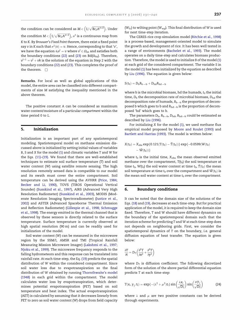
5. Initialization

Initialization is an important part of any spatiotemporal

modeling. Spatiotemporal model on methane emission dis-

cussed above is initialized by setting initial values of variables

B, S and X for the model (1) and climatic variables T and W for

the Eqs. (11)–(19). We found that there are well-established

techniques to estimate soil surface temperature (T) and soil

water content (W) using satellite remote sensing. The high

resolution remotely sensed data is compatible to our model

and its swath must cover the entire compartment. Soil

temperature can be derived using the AVHRR (Price, 1984;

Becker and Li, 1990), TOVS (TIROS Operational Vertical

Sounder) (Susskind et al., 1997), AIRS (Advanced Very High

Resolution Radiometer) (Susskind et al., 2003), MODIS (Mod-

erate Resolution Imaging Spectroradiometer) (Justice et al.,

2002) and ASTER (Advanced Spaceborne Thermal Emission

and Reflection Radiometer) (Gillespie et al., 1998; Schmugge

et al., 1998). The energy emitted in the thermal channel that is

observed by these sensors is directly related to the surface

temperature. Surface temperature is currently observed at

high spatial resolution (90 m) and can be readily used for

initialization of the model.

Soil water content (W) can be measured in the microwave

region by the SSM/I, AMSR and TMI (Tropical Rainfall

Measuring Mission Microwave Imager) (Lakshmi et al., 1997;

Njoku et al., 1999). The microwave frequency responds to the

falling hydrometeors and this response can be translated into

rainfall rate. At each time-step, the Eq. (19) predicts the spatial

distribution of W within the considered compartment. Since

soil water loss due to evapotranspiration so the final

distribution of W obtained by running Thornthwaite’s model

(1948) in each grid within the compartment. The model

calculates water loss by evapotranspiration, which deter-

mines potential evapotranspiration (PET) based on soil

temperature and heat index. The actual evapotranspiration

(AET) is calculated by assuming that it decreases linearly from

PET to zero as soil water content (W) drops from field capacity

(Wfc) to wilting point (Wwp). This final distribution of W is used

for next time-step iteration.

The CERES-rice crop simulation model (Ritchie et al., 1998)

is a process-based, management-oriented model to simulate

the growth and development of rice. It has been well tested in

a range of environments (Bachelet et al., 1993). The model

operates on a daily time-step and calculates biomass produc-

tion. Therefore, the model is used to initialize B of the model (1)

at each grid of the considered compartment. The variable S in

the model (1) has been initialized by the equation as described

by Liu (1996). The equation is given below:

Sðt0Þ ¼ DbRb!b þ DhdRhd!b

where b is the microbial biomass, hd the humads, t0 the initial

time, Db the decomposition rate of microbial biomass, Dhd the

decomposition rate of humads, Rb!b the proportion of decom-

posed b which goes to b and Rhd!b is the proportion of decom-

posed ‘hd’ which goes to b.

The parameters Db, Rb!b, Dhd, Rhd!b could be estimated as

described by Liu (1996).

For initializing X for the model (1), we used methane flux

empirical model proposed by Moore and Roulet (1993) and

Bartlett and Harriss (1993). The model is written below:

Xðt0Þ ¼ Xobs expf0:121ðTðt0Þ � Tðt0ÞÞg expf�0:0599ðWðt0Þ

� Wðt0ÞÞg

where t0 is the initial time, Xobs the mean observed emitted

methane over the compartment, T(t0) the soil temperature at

time t0, W(t0) the soil water content at time t0, Tðt0Þ the mean

soil temperature at time t0 over the compartment and Wðt0Þ is

the mean soil water content at time t0 over the compartment.

6. Boundary conditions

It can be noted that the domain size of the solutions of the

Eqs. (18) and (19), decreases at each time-step. But for practical

application of the model, it is required to keep the domain size

fixed. Therefore, T and W should have different dynamics on

the boundary of the spatiotemporal domain such that the

iteration scheme for predicting T and W at each time-step does

not depends on neighboring grids. First, we consider the

spatiotemporal dynamics of T on the boundary, i.e. general

diffusion equation of heat transfer. The equation is given

below:

@T@t¼ DT

@2T@x2þ @2T

@y2

� �

where DT is diffusion coefficient. The following discretized

form of the solution of the above partial differential equation

predicts T at each time-step:

Tðxi; y j; tlÞ ¼ expf�ðl2 þ m2Þtlg sinlxiffiffiffiffiffiffiDTp� �

sinmy jffiffiffiffiffiffi

DTp� �

(24)

where l and m are two positive constants can be derived

through experiments.

e c o l o g i c a l c o m p l e x i t y 3 ( 2 0 0 6 ) 2 3 1 – 2 4 0238

The water balance equation is considered on the boundary

of spatiotemporal domain. The equation is written below:

Wðxi; y j; tl þ kÞ ¼Wðxi; y j; tlÞ þ Winput �WoutputÞ ��

ðxi ;y j ;tlÞk (25)

where Winput is the water added from rainfall and Woutput is the

evaporated water calculated using Thornthwaite’s model

(1948).

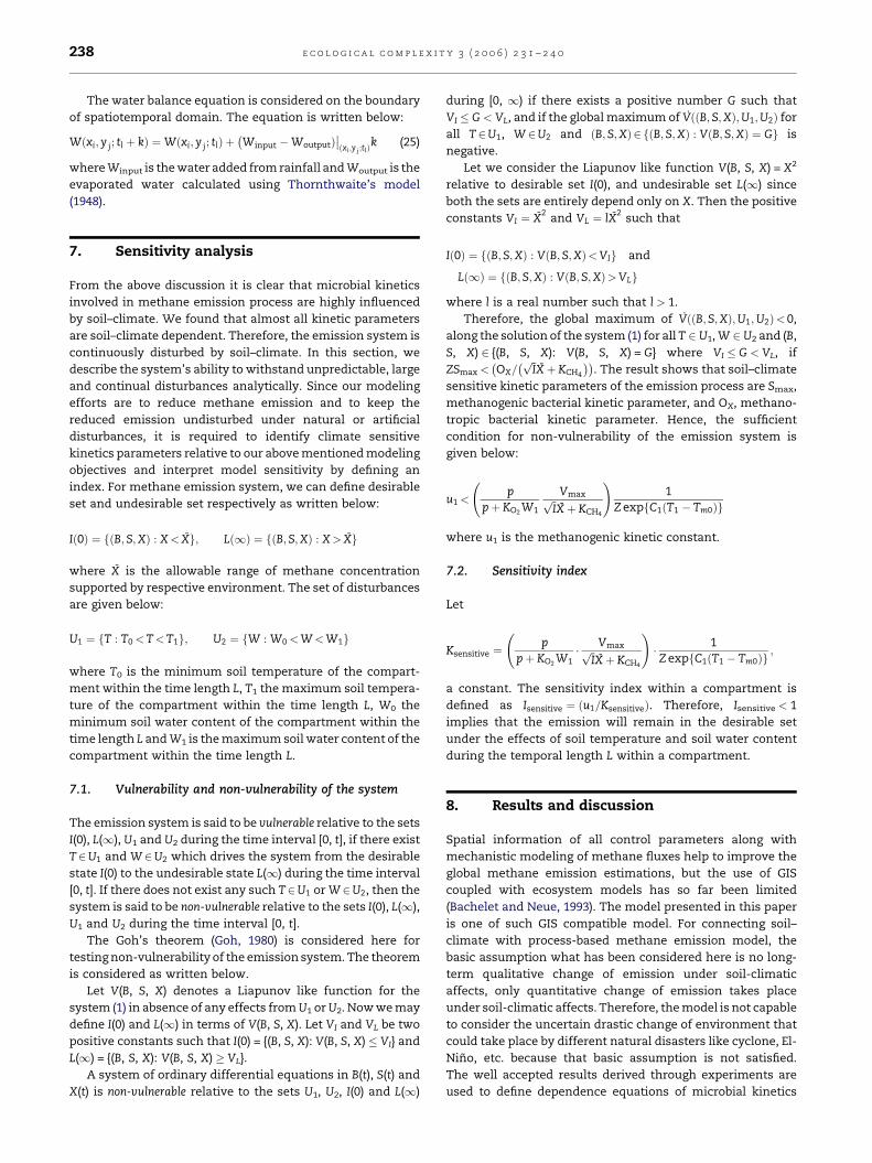
7. Sensitivity analysis

From the above discussion it is clear that microbial kinetics

involved in methane emission process are highly influenced

by soil–climate. We found that almost all kinetic parameters

are soil–climate dependent. Therefore, the emission system is

continuously disturbed by soil–climate. In this section, we

describe the system’s ability to withstand unpredictable, large

and continual disturbances analytically. Since our modeling

efforts are to reduce methane emission and to keep the

reduced emission undisturbed under natural or artificial

disturbances, it is required to identify climate sensitive

kinetics parameters relative to our above mentioned modeling

objectives and interpret model sensitivity by defining an

index. For methane emission system, we can define desirable

set and undesirable set respectively as written below:

Ið0Þ ¼ fðB; S;XÞ : X< Xg; Lð1Þ ¼ fðB;S;XÞ : X> Xg

where X is the allowable range of methane concentration

supported by respective environment. The set of disturbances

are given below:

U1 ¼ fT : T0 <T<T1g; U2 ¼ fW : W0 <W<W1g

where T0 is the minimum soil temperature of the compart-

ment within the time length L, T1 the maximum soil tempera-

ture of the compartment within the time length L, W0 the

minimum soil water content of the compartment within the

time length L and W1 is the maximum soil water content of the

compartment within the time length L.

7.1. Vulnerability and non-vulnerability of the system

The emission system is said to be vulnerable relative to the sets

I(0), L(1), U1 and U2 during the time interval [0, t], if there exist

T2U1 and W2U2 which drives the system from the desirable

state I(0) to the undesirable state L(1) during the time interval

[0, t]. If there does not exist any such T2U1 or W2U2, then the

system is said to be non-vulnerable relative to the sets I(0), L(1),

U1 and U2 during the time interval [0, t].

The Goh’s theorem (Goh, 1980) is considered here for

testing non-vulnerability of the emission system. The theorem

is considered as written below.

Let V(B, S, X) denotes a Liapunov like function for the

system (1) in absence of any effects from U1 or U2. Now we may

define I(0) and L(1) in terms of V(B, S, X). Let VI and VL be two

positive constants such that I(0) = {(B, S, X): V(B, S, X) � VI} and

L(1) = {(B, S, X): V(B, S, X) � VL}.

A system of ordinary differential equations in B(t), S(t) and

X(t) is non-vulnerable relative to the sets U1, U2, I(0) and L(1)

during [0, 1) if there exists a positive number G such that

VI � G < VL, and if the global maximum of VððB; S;XÞ;U1;U2Þ for

all T2U1, W2U2 and ðB; S;XÞ 2 fðB;S;XÞ : VðB;S;XÞ ¼ Gg is

negative.

Let we consider the Liapunov like function V(B, S, X) = X2

relative to desirable set I(0), and undesirable set L(1) since

both the sets are entirely depend only on X. Then the positive

constants VI ¼ X2

and VL ¼ lX2

such that

Ið0Þ ¼ fðB; S;XÞ : VðB; S;XÞ<VIg and

Lð1Þ ¼ fðB;S;XÞ : VðB;S;XÞ>VLg

where l is a real number such that l > 1.

Therefore, the global maximum of VððB;S;XÞ;U1;U2Þ<0,

along the solution of the system (1) for all T 2 U1, W 2 U2 and (B,

S, X) 2 {(B, S, X): V(B, S, X) = G} where VI � G < VL, if

ZSmax < OX=ffiffiIp

Xþ KCH4

� �. The result shows that soil–climate

sensitive kinetic parameters of the emission process are Smax,

methanogenic bacterial kinetic parameter, and OX, methano-

tropic bacterial kinetic parameter. Hence, the sufficient

condition for non-vulnerability of the emission system is

given below:

u1 <p

pþ KO2 W1

VmaxffiffiIp

Xþ KCH4

!1

Z expfC1ðT1 � Tm0Þg

where u1 is the methanogenic kinetic constant.

7.2. Sensitivity index

Let

Ksensitive ¼p

pþ KO2 W1� Vmaxffiffi

Ip

Xþ KCH4

!� 1Z expfC1ðT1 � Tm0Þg

;

a constant. The sensitivity index within a compartment is

defined as Isensitive ¼ ðu1=KsensitiveÞ. Therefore, Isensitive < 1

implies that the emission will remain in the desirable set

under the effects of soil temperature and soil water content

during the temporal length L within a compartment.

8. Results and discussion

Spatial information of all control parameters along with

mechanistic modeling of methane fluxes help to improve the

global methane emission estimations, but the use of GIS

coupled with ecosystem models has so far been limited

(Bachelet and Neue, 1993). The model presented in this paper

is one of such GIS compatible model. For connecting soil–

climate with process-based methane emission model, the

basic assumption what has been considered here is no long-

term qualitative change of emission under soil-climatic

affects, only quantitative change of emission takes place

under soil-climatic affects. Therefore, the model is not capable

to consider the uncertain drastic change of environment that

could take place by different natural disasters like cyclone, El-

Nino, etc. because that basic assumption is not satisfied.

The well accepted results derived through experiments are

used to define dependence equations of microbial kinetics

e c o l o g i c a l c o m p l e x i t y 3 ( 2 0 0 6 ) 2 3 1 – 2 4 0 239

parameters. Though oxidation rate of produced methane due to

the activity of methanotropic bacteria is considered as a

function of W only but as other microbial kinetics parameters,

it may also depends on T. In literature we have not found such

experimentally derived results by which we can construct a

dependence equation for OX depends on T and W both. It may be

possible to consider different dependence equations based on

different experiments but the modeling framework, i.e.

spatiotemporal domain remains fixed. Spatial variation of soil

temperature and soil water content occurs even in very small

spatial scale. Therefore, when we consider grid size, h small

enough strengthens the model to capture the spatial hetero-

geneity explicitly. But it makes the model less practicable even

though compartment-wise model simulation is carried out.

Therefore, small-scale applications of this model will produce

better result. Seasonal methane emission pattern and dial

methane emission pattern can be extracted by adjusting the

measurements of model parameters relative to adjusted

temporal length, L. Soil water flow depends on soil depth and

also soil temperature varies with respect to soil depth. The

model could be modified by incorporating the effects of soil

depth on the spatiotemporal dynamics of soil temperature and

soil water content. The importance of this modeling efforts are,

the model is capable to identify emission sources and those

sources having out-busting emission tendency in long-term

with respect to space and time and what should be the strategy

for reducing emission level has been discussed by Chakraborty

and Bhattacharya (2006a). The following steps for computation

have been proposed based on discussions in above sections:

Step 1: Classifying the entire study area (rice fields) into

compartments of size M satisfying the inequality men-

tioned in Theorem 1 and dividing each compartment into

small grids.

Step 2: Extracting spatial patterns of T and W from high

resolution remotely sensed data for model initialization

such that its spatial resolution should match with fixed grid

size.

Step 3: Determining spatial distribution of kinetic para-

meters with same spatial resolution.

Step 4: Calculating X(t) at each grid by solving ordinary

differential equations based on system (1) numerically at

each time-step and identifying permanent emission grids

having X(t) > 0 for all time-steps within the considered

temporal length L.

Step 5: Identifying out-busting emission grids by calculating

emission indices (Chakraborty and Bhattacharya, 2006a,b)

at each identified permanent emission grid and checking

either X(t), X*> or < X where X* is emitted methane

concentration at equilibrium of the system (1) if exists.

The last step is for decision making on what control

measure has to adopt to reduce methane emission under

complex and uncertain situations.

Acknowledgements

We are thankful to Prof. A.B. Roy of Jadavpur University, India

for his valuable suggestions. This work was partially sup-

ported by UC Agricultural Experiment Station and U.S.

National Science Foundation.

r e f e r e n c e s

Bachelet, D., Neue, H.U., 1993. Methane emissions from wetlandrice areas of Asia. Chemosphere 26, 219–237.

Bachelet, D., Van Sickle, J., Gay, C.A., 1993. The impacts ofclimate change on rice yield: evaluation of the efficacy ofdifferent modeling approaches. In: Penning de Vries,F.W.T., Teng, P.S., Metselaar, K. (Eds.), SystemsApproaches for Agricultural Development. KluwerAcademic Publishers, Dordrecht, The Netherlands, pp.145–174.

Bartlett, K.B., Harriss, R.C., 1993. Review and assessment ofmethane emissions from wetlands. Chemosphere 26, 261–320.

Becker, F., Li, Z., 1990. Towards a local split window methodover land surfaces. Int. J. Remote Sensing 11, 369–393.

Chakraborty, A., Bhattacharya, D.K., 2006a. A process basedmodel on methane emission with its oxidation processfrom rice fields and corresponding control indices. J.Environ. Model. Assess. (submitted for publication).

Chakraborty, A., Bhattacharya, D.K., 2006b. A process basedmathematical model on methane production with emissionindices for control. Bull. Math. Biol., doi:10.1007/s11538-006-9076-x.

Chen, Y.R., Varel, V.H., Hashimoto, A.G., 1980. Effect oftemperature on methane fermentation kinetics of beef-cattle manure. Biotechnol. Bioeng. Symp. 10, 325–339.

Clapp, R.B., Hornberger, G.M., 1978. Empirical equations forsome soil hydraulic properties. Water Resour. Res. 14, 601–604.

Cunnold, D., Prinn, R., Rasmussen, R., Simmonds, P., Alyea, F.,Cardelino, C., Crawford, A., Fraser, P., Rosen, R., 1986. Theatmospheric lifetime and annual release estimates for CFCl3and CF2Cl2 from 5 years of ALE data. J. Geophys. Res. 91,10797–10817.

Cunnold, D., Prinn, R., Rasmussen, R., Smmonds, P., Alyea, F.,Cardelino, C., Crawford, A., Fraser, P., Rosen, R., 1983. Theatmospheric lifetime experiment 3, lifetime methodologyand application to three years of CFCl3 data. J. Geophys. Res.88, 8379–8400.

DeVries, D.A., 1975. Heat transfer in soils. In: DeVries, D.A.,AfganHeat, N.H. (Eds.), Mass Transfer in the Biosphere, vol.1. John Wiley, New York.

Endo, G., Noike, T., Matsumoto, J., 1983. Effect of temperatureand pH on acidogenic phase in anaerobic digestion. Proc.Japan Soc. Civil Eng. 330, 49–57.

Fung, I., John, J., Lerner, J., Matthews, E., Prather, M., Steele, L.P.,Fraser, P.J., 1991. Three-dimensional model synthesis of theglobal methane cycle. J. Geophys. Res. 96, 13033–13065.

Gillespie, A., Cothern, J.S., Rokugawa, S., Matsunaga, T., Hook,S.J., Kahle, A.B., 1998. A temperature and emissivityseparation algorithm for advanced spaceborn thermalemission and reflection radiometer (ASTER) images. IEEETrans. Geosci. Remote Sensing 36 (4), 1113–1126.

Godwin, D.C., Jones, C.A., 1991. Nitrogen dynamics in soil plantsystems. In: Hanks, J., Ritchie, JT. (Eds.), Modeling Soil, Plant,Systems, Agron Soc Am, Madison, pp. 287–322.

Goh, B.S., 1980. Management and Analysis of BiologicalPopulations. Elsevier, Amsterdam.

Hartley, D., Prinn, R., 1993. Feasibility of determining surfaceemissions of trace gases using an inverse method in athree-dimensional chemical transport model. J. Geophys.Res. 98, 5183–5198.

e c o l o g i c a l c o m p l e x i t y 3 ( 2 0 0 6 ) 2 3 1 – 2 4 0240

Hashimoto, A.G., 1982. Methane from cattle waste: effects oftemperature, hydraulic retention time and influentsubstrate concentration on kinetic parameter (K).Biotechnol. Bioeng. 24, 2039–2052.

Huwe, B., 1997. SOHE: a numerical model for the simulation ofheat flux in soils. Abteilung Bodenphysik, UniversitatBayreuth.

Justice, O., Townshend, J.R.G., Vermote, E.F., Masuoka, E., Wolfe,R.E., Saleous, N., Roy, D.P., Morisette, J.T., 2002. An overviewof MODIS land data processing and product status. RemoteSensing Environ. 83 (12), 3–15.

Lakshmi, V., Wood, E.F., Choudhury, B.J., 1997. A soil canopy-atmosphere model for use in satellite microwave remotesensing. J. Geophys. Res. 102 (D6), 6911–6927.

Lawrence, A.W., McCarty, P.L., 1969. Kinetics of methanefermentation in anaerobic treatment. J. Water Poll. ControlFed. 41, R1–R17.

Liu, Y., 1996. Modeling the emission of nitrous oxide (N2O) andmethane (CH4) from the terrestrial biosphere to theatmosphere. PhD Thesis. MIT Joint Program on the Scienceand Policy of Global Change. MIT, Cambridge, MA, USA.

Mahowald, N.M., 1996. Development of a 3-dimensionalchemical transport model based on observed winds and usein inverse modeling of the sources of CCl3F. PhD Thesis.MIT, Cambridge, MA.

Matthews, R.B., Wassmann, R., Arah, J., 2000. Using a crop/soilsimulation model and GIS techniques to assess methaneemission from rice fields in Asia. 1. Model development.Nutr. Cycl. Agro-Ecosyst. 58, 141–159.

Moore, T.R., Roulet, N.T., 1993. Methane flux: water table relationsin Northern Wetlands. Geophys. Res. Lett. 20, 587–590.

Nagase, M., Matsuo, T., 1982. Interactions between amino-acid-degrading bacteria and methanogenic bacteria in anaerobicdigestion. Biotechnol. Bioeng. 24, 2227–2239.

Nagumo, M., 1942. Uberdie lage der Integrakurven gewonlicherDifferantial gleichungen. Proc. Phys. Math. Soc. Japan 24,551–559.

Neue, H.U., Boonjwat, J., 1993. Methane emission from ricefields. Bioscience 43 (7), 466–475.

Njoku, G., Jackson, T., Lakshmi, V., Chan, T., Nghiem, S., 1999.Soil moisture retrieval from AMSR-E. IEEE Trans. Geosci.Remote Sensing 37, 79–93.

Novak, J.T., 1974. Temperature–substrate interaction in biologicaltreatment. J. Water Poll. Control Fed. 46, 1984–1994.

O’Rourke, J.T., 1968. Kinetics of anaerobic treatment atreduced temperatures. Thesis presented to StanfordUniversity in partial fulfillment of the requirementfor the degree of Doctor of Philosophy: Cited byLawrence A. W. 1971. Application of process kinetics todesign of anaerobic processes. Adv. in Chemistryseries 105, 163–189.

Oremland, R., Culbertson, C., 1992. Importance of methaneoxidizing bacteria in the methane budget as revealed by useof specific inhibitor. Nature 356, 421–423.

Price, C., 1984. Land surface temperature measurementsfrom the split window channels of the NOAA-7 advancedvery high resolution radiometer. J. Geophys. Res. 89,7231–7237.

Prinn, R., Cunnold, D., Rasmussen, R., Simmonds, P., Alyea, F.,Crawford, A., Fraser, P., Rosen, R., 1990. Atmosphericemissions and trends of nitrous oxide deduced from 10years of ALE/GAGE data. J. Geophys. Res. 95, 18369–18385.

Ritchie, J.T., Singh, U., Godwin, D.C., Bowen, W.T., 1998. Cerealgrowth, development and yield. In: Tsuji, G., Hoogenboom,G., Thornton, P. (Eds.), Understanding Operations forAgricultural Development. Kluwer Academic Publishers,Dordrecht, The Netherlands, pp. 79–98.

Schmugge, T., Hook, S.J., Coll, C., 1998. Recovering surfacetemperature and emissivity from thermal infraredmultispectral data. Remote Sensing Environ 65 (2), 121–131.

Siebelt, M.L., Toerien, D.F., 1969. The proteolytic bacteriapresent in the anaerobic digestion of raw sewage sludge.Water Res. 3, 241–250.

Stein, V.B., Hettiaratchi, J.P.A., Achari, G., 2001. Numericalmodels for biological oxidation and migration of methanein soils. Practice periodical of hazardous. Toxic RadioactiveWaste Manage. 5, 225–234.

Susskind, J., Barnet, C., Blaisdell, J., 2003. Retrival of atmosphericand near surface parameters from AIRS/AMSU/HSB data inthe presence of clouds. IEEE Trans. Geosci. Remote Sensing41 (2), 390–409.

Susskind, J., Piraino, P., Rokke, L., Iredell, L., Mehta, A., 1997.Characteristic of the TOVS Pathfinder path A data set. Bull.Am. Meteorol. Soc. 78 (7), 1449–1472.

Thornthwaite, W., 1948. An approach toward a rationalclassification of climate. Geogr. Rev. 38, 55–89.

Topiwala, H., Sinclair, C.G., 1971. Temperature relationship incontinuous culture. Biotechnol. Bioeng. 13, 795–813.